Machine Learning versus Mathematical Model to Estimate the

Machine Learning versus Mathematical Model to Estimate the

Transverse Shear Stress Distribution in a Rectangular Channel

Babak Lashkar-Ara 1,*, Niloofar Kalantari 1, Zohreh Sheikh Khozani 2 and Amir Mosavi 2,3,4,*

1 Department of Civil Engineering, Jundi-Shapur University of Technology, 64616-18674 Dezful, Iran; 2 Institute of Structural Mechanics, Bauhaus Universität-Weimar, 99423 Weimar, Germany;

[email protected] 3 School of Economics and Business, Norwegian University of Life Sciences, 1430 Ås, Norway 4 John von Neumann Faculty of Informatics, Obuda University, 1034 Budapest, Hungary

* Correspondence: [email protected] (B.L.-A.); [email protected] (A.M.)

Abstract: One of the most important subjects of hydraulic engineering is the reliable estimation of

the transverse distribution in the rectangular channel of bed and wall shear stresses. This study

makes use of the Tsallis entropy, genetic programming (GP) and adaptive neuro-fuzzy inference

system (ANFIS) methods to assess the shear stress distribution (SSD) in the rectangular channel. To

evaluate the results of the Tsallis entropy, GP and ANFIS models, laboratory observations were

used in which shear stress was measured using an optimized Preston tube. This is then used to

measure the SSD in various aspect ratios in the rectangular channel. To investigate the shear stress

percentage, 10 data series with a total of 112 different data for were used. The results of the sensi-

tivity analysis show that the most influential parameter for the SSD in smooth rectangular channel

is the dimensionless parameter B/H, Where the transverse coordinate is B, and the flow depth is H.

With the parameters (b/B), (B/H) for the bed and (z/H), (B/H) for the wall as inputs, the modeling of

the GP was better than the other one. Based on the analysis, it can be concluded that the use of GP

and ANFIS algorithms is more effective in estimating shear stress in smooth rectangular channels

than the Tsallis entropy-based equations.

Keywords: smooth rectangular channel; Tsallis entropy; genetic programming; artificial intelli-

gence; machine learning; big data; computational hydraulics; neuro-fuzzy; data science

1. Introduction

Knowledge of boundary shear stress is necessary when studying sediment transport,

flow pattern around structures, estimation of scour depth and channel migration. The de-

termination of boundary shear stress, i.e., at the wall and bed depends on the channel

geometry and its associated roughness. Various direct and indirect methods have been

extensively discussed in experimentally measure the wall and bed shear stresses in chan-

nels with different cross sections [1–4]. Bed shear stress can be estimated based on four

techniques (1) bed slope product 𝜏𝑏 = g𝐻𝑆 , (2) law of the wall velocity profiles 𝑢

𝑢∗=

1

𝑘𝑙𝑛 (

𝑧

𝑧0) where 𝜏𝑏 = 𝜌𝑢∗

2, (3) Reynolds stress measurement 𝜏𝑏 = 𝜌(−𝑢′𝑤′) and (4) turbu-

lent kinetic energy (TKE), TKE =𝜌(𝑢′2+𝑣′2+𝑤′2)

2, where 𝜏𝑏 = 𝐶1TKE , where 𝑢′, 𝑣′ and 𝑤′

are the fluctuating horizontal, transversal and vertical velocity components, respectively

and 𝐶1 = 0.20 [5]. The symbols g, H and S denote gravity, water level and channel slope,

respectively, whereas 𝑢 is the velocity at height z, 𝑢∗ is the shear velocity, k is von Kar-

man constant and 𝑧0 is the roughness length.

These methods are useful in presenting a point-based representation of shear stress

in a channel, whereas the shear stress distribution (SSD) provides a more accurate hydro-

dynamic profile within a channel. Knight and Sterling [6] measured the SSD in a circular

channel with and without sediment. They examined a wide range of flow depths for each

level benching and therefore it had been possible to determine the extent to which the

hydraulics changes Park et al. [7] utilized laboratory-scale water flume and measured the

bed shear stress under high-velocity flow conditions directly. Lashkar-Ara and Fatahi [8]

measured transverse SSD in the channel bed and wall by using an optimal diameter Pres-

ton tube to evaluate the SSD on a rectangular open channel. The outcome of this research

is two-dimensional relationships to evaluate local shear stress in both bed and wall. The

bed and wall relative coordinates b/B and z/H in the cross section also the aspect ratio B/H

are the function of these relationships. The study showed that the dimensionless SSD is

greatly affected by the aspect ratio. Utilizing the advantages offered in the soft computing

method and the artificial intelligence (AI) techniques, other researchers have been ex-

tended numerically and analytically to overcome difficulties with experimental measure-

ments [9–12]. Martinez-Vazquez and Sharifi [13] utilized recurrence plot (RP) analysis and

eigenface for recognition to estimate the SSD in trapezoidal and circular channels. A new

approach has been developed by Sterling and Knight [14] to estimate the SSD in a circular

open channel. In terms of accuracy, the analysis showed that there is a lack of ability in

the outcome and it is not satisfactory. The uncertainty of the estimation of the model pa-

rameters and the high sensitivity of the outcomes to the expected experiment parameters

can be due to this. Sheikh Khozani and Bonakdari [15] extended the analytical method

based Renyi entropy to estimate SSD in circular channels. Sheikh Khozani and Bonakdari

[16] researched on the comparison of five different models in straight compound channel

prediction of SSD. In other research, Sheikh Khozani and Wan Mohtar [10] analyzed the

formulation of the SSD on the basis of the Tsallis entropy in circular and trapezoidal chan-

nels. Sheikh Khozani et al. [17] have attempted in another study to use an improved SVM

method to estimate shear stress in rough rectangular channel.

Ardiҫlioğlu et al. [18], conducted an experimental study for the SSD throughout the

entire length of the cross-section in fully developed boundary layer area, in an open rec-

tangular channel, in both smooth and rough surface. By measuring the speed in both

smooth and rough surfaces, they conducted tests. Using logarithmic distribution of veloc-

ity, the average shear stresses in the cross section for aspect ratios of 4.2–21.6 and the

Froude numbers of 0.12–1.23 were measured. The definition of the Tsallis entropy was

used by Bonakdari et al. [19] to predict the SSD in trapezoidal and circular channels and

achieve acceptable accuracy. Although the direct measurement of shear stress in labora-

tory provides correct description of the spatial pattern, the measurement of shear stress

using shear place or cell is laborious, complex, requires careful calibration and may not

applicable to all type of channels [20]. The use of soft computing techniques in the simu-

lation of engineering problems was intensively studied and a variety of soft computing

methods were suggested. To approximate the daily suspended sediment load, Kisi et al.

[21] used a genetic programming (GP) model. They also contrasted this approach with

various machine learning methods and concluded that the GP model works better than

the others. In estimating SSD in circular channels with and without flat-bed Sheikh

Khozani et al. [22,23] applied randomize neural network (RNN) and gene expression pro-

gramming (GEP). In this study, the Tsallis entropy was used to determine SSD in a smooth

bed and wall in a rectangular open channel. This is then used to measure the SSD in vari-

ous aspect ratios in the rectangular channel. In the second part of the study, two soft com-

puting methods were applied to predict the transverse of SSD in the smooth rectangular

channel. The methods of genetic programming (GP) and the adaptive neuro-fuzzy infer-

ence system (ANFIS) were examined to determine the precision of these models in esti-

mating bed and wall shear stress. This study aimed at using the Tsallis entropy method

to predict the SSD in the smooth rectangular channel. The results of the Tsallis entropy,

GP and ANFIS methods compared with experimental results of Lashkar-Ara and Fatahi

[8]. Although this analysis was performed in parallel with Sheikh Khozani and Bonakdari

[16] research, it can be said in a practical contrast that the data used in this study is based

on the measurement of shear stress using the optimal diameter of the Preston tube, which

was designed by Lashkar-Ara and Fatahi [8], so the comparison of findings is more precise

and less uncertain.

2. Materials and Methods

2.1. Data Collection

Information on the SSD was collected in the Lashkar-Ara and Fatahi [8] experiments

of a smooth rectangular channel, performed in a flume 10-meter long, 60 cm wide and 70

cm high. All measurements were performed in the range of 11.06–102.38 liter per second

flow rate. Flow rate variations led to observable changes in water depth ranging from 4.3

to 21 cm and the aspect ratio of 2.86–13.95. The values of static and total pressure differ-

ence in various aspect ratios of B/H were measured and reported using pressure trans-

ducer apparatus with a capacity of 200 mill bar and 50 Hz measuring frequency. In order

to create uniform flow condition and to match the hydraulic gradient with the flume bed

slope a weir at the end of the flume was installed. Figure 1 illustrates the notation used

for a smooth rectangular channel conduit. Figure 2 shows the schematic of experimental

setup.

Figure 1. Schematics of local shear stress distribution coordinates in the rectangular channel wall and bed.

Figure 2. Experiment schematic.

Based on previous studies in the laboratory and field investigation, the effective cri-

teria for evaluating the SSD along the wet periphery of a channel can be expressed as

follows:

( )1 ,ρ ,υ ,g , , , , , , , 0=w w o sf V H S S B z K (1)

( )2 ,ρ ,υ ,g , , , , , , , 0=b w o sf V H S S B b K (2)

where �̄�𝑤 is the average wall shear stress, �̄�𝑏 is the average bed shear stress, 𝜌 is the

density, υ is the kinematic viscosity, g is the gravity acceleration, V is the flow velocity, H

is the flow depth, B is the flume bed width, Sw is the water surface slope, 𝑘𝑠 is the rough-

ness height, (Re) is the Reynolds number and (Fr) is the Froude number.

The Buckingham-π theorem is used to obtain independent dimensional parameters

for wall and bed shear stress, as shown in Equations (3) and (4).

3 2

w 0zυ g

, , , , ,ρg

=

s

w

K H Bf

VH H H H HSV

(3)

4 2

bυ g, , , , , 0

ρg

=

s

w

K H B bf

VH H H B HSV

(4)

In the case of smooth channel equations (3) and (4) can be rewritten as (5) and (6):

w

5

2Re,Fr , ,ρg

=

w

B zf

HS H H

(5)

2

6 Re,Fr , ,ρg

=

b

w

B bf

HS H B

(6)

For GP simulation, 160 data of bed shear stress (τb) and 100 data of wall shear stress

(τw) were collected in a smooth rectangular channel with different flow depths. Approxi-

mately 70 percent of the total data were chosen for training and the remaining 30 percent

for testing. The summary of experiments is tabulated in Table 1.

Table 1. Experimental summary.

Parameters Variable Definition Minimum Maximum Mean

H (m) Flow depth 0.043 0.21 0.0928

B/H aspect ration 2.86 13.95 7.98

Q (L/s) Discharge 11.06 102.38 34.795

V (m/s) Velocity 0.429 0.813 0.568

Fr Froude number 0.66 0.566 0.618

Re × 104 Reynolds number 6.4 39.87 16.418

*Re Shear Reynolds 0.322 0.609 0.426

HS Total shear stress 0.442 2.162 0.955

2.2. Tsallis Entropy

If a random variable (τ) in a cross section of a channel is assumed to be a consistent

shear stress, then, according to Tsallis entropy of [24] the SSD or shear stress probability

density function f(τ), can be identified as [19]:

max 1

0

1( ) ( )(1 ( ) ) d

1

−= −−

qH f fq

(7)

where τ is the shear stress, q is a true number, and Tsallis 's entropy function is H(τ). The

τ value varies from 0 to τmax, and with these restrictions, the integral value of H(τ) will be

1.

Using the maximum entropy theorem, the f(τ) can be calculated to maximize the en-

tropy function subject to specified constraints like Equations (8) and (9) respectively [25].

max

0( )d 1= f

(8)

max

0. ( )d = f

(9)

where the mean and maximum shear stress values are �̄� and τmax, respectively.

At this stage, using maximization of Lagrange coefficients by Equations (7)–(9), the

Lagrange function L can be written down as Equation (10):

( ) ( )max max max1

0 10 0 0

( )(1 ( ) )d ( ) 1 . ( )d

1

−= − + − + −−

qfL f f d f

q

(10)

where λ0 and λ1 are the Lagrange multipliers. By ∂L/∂(τ) = 0 to maximize entropy, the f(τ)

yields as:

𝑓(𝜏) = [𝑞 − 1

𝑞(λ′ + λ1. 𝜏)]

1(𝑞−1)

(11)

where 𝜆′ =1

𝑞−1+ 𝜆0. In Equation (10), the shear stress probability distribution func-

tion (PDF) is represented by f(τ). The SSD's cumulative distribution function (CDF) is in-

troduced as Equation (12):

𝐹(𝜏) = ∫ 𝑓(𝜏)𝑑𝜏 =𝑦

𝐿

𝜏𝑚𝑎𝑥∫

0

(12)

where y is the direction of the channel wall, which varies from 0 at the free surface to L,

and L is the entire wetted perimeter. The function of f(τ) is the derivative of F(τ), so a

partial derivation of F(τ) with respect to y is carried out in the following equation:

𝑓(𝜏) =d𝐹(𝜏)

d𝑢=

1

𝐿

d𝑦

d𝜏 (13)

By substituting Equation (11) into Equations (12) and (13) and solving the integral

and simplifying, the shear stress function is represented as Equation (14).

𝜏 =𝑘

𝜆1

[(𝜆′

𝑘)𝑘 +

𝜆1𝑦

𝐿]

1𝑘

−𝜆′

𝜆1

(14)

where k = q/q − 1 and q value is the constant of ¾ according to [10,26], which is defined as

the parameter of the Tsallis relationship. λ1 and λ′ are Lagrange multipliers that can be

derived by trial and error from two implicit equations that follow. Indeed, by inserting

and integrating Equation (10) into two constraints (Equations (8) and (9)), two Equations

(15) and (16) are returned as:

kk k

1 max 1λ λ λ λ k + − = (15)

𝜏𝜆1 [𝜆′ + 𝜆1𝜏𝑚𝑎𝑥[]𝑘 [𝜆′ + 𝜆1𝜏𝑚𝑎𝑥[]k+1[𝜆′]k+1

𝑘𝜆12𝑘�̄�]]

𝑚𝑎𝑥 (16)

Equations (15) and (16) solve to obtain two undefined Lagrange multipliers (λ1 and

λ′). To estimate the SSD, a pair of mean and maximum shear stresses is required. The

results of the Lashkar-Ara and Fatahi [9] studies have been used for this reason in order

to estimate the values of τmax and �̄� . They adjusted the slope of the bed flume at

9.58 × 10−4. The shear stress carried by the walls and bed was measured for a different

aspect ratio (B/H = 2.86, 4.51, 5.31, 6.19, 7.14, 7.89, 8.96, 10.71, 12.24 and 13.95). For each

aspect ratio, the distribution of shear stress in the bed and wall was measured by a Preston

tube. The best fit equation was obtained for τmax and �̄� separately for wall and bed in as-

pect ratio 2.89 < B/H < 13.95 by assuming a fully turbulent and subcritical regime among

all the experimental results. Relationships are shown in Equations (17)–(20).

�̄�𝑤

ρg𝑅𝑆=

2.1007 + 0.0462 (𝐵𝐻

)

1 + 0.1418 (𝐵𝐻

) + (𝐵𝐻

)−0.0424 (17)

�̄�𝑏

ρg𝑅𝑆=

2.0732 − 0.0694 (𝐵𝐻

)

1 − 0.146 (𝐵𝐻

) + (𝐵𝐻

)−0.1054 (18)

𝜏𝑚𝑎𝑥 𝑤

ρg𝑅𝑆=

2.5462 + 6.5434 (𝐵𝐻

)

1 + 6.34 (𝐵𝐻

) + (𝐵𝐻

)−0.1083 (19)

𝜏𝑚𝑎𝑥 𝑏

ρg𝑅𝑆=

3.157 + 0.8214 (𝐵𝐻

)

1 + 0.8535 (𝐵𝐻

) + (𝐵𝐻

)−0.1401 (20)

where �̄�𝑤&�̄�𝑏 and 𝜏max 𝑤 and 𝜏max 𝑏are the mean and maximum shear stress on the chan-

nel wall and bed, respectively. Therefore, the transverse SSD for the rectangular open

channel can be determined depending on the aspect ratio and the slope of the channel

bed.

2.3. Genetic Programming (GP)

In the second part of this analysis, the GP model is applied as one of the evolutionary

algorithms (EA) to improve the accuracy of the given relations. The GP is an automated

programming method to solve problems by designing computer programs GP is widely

used for modeling structure recognition technology applications concerns. For this aim

the GP technique was used to understand the basic structure of a natural or experimental

process. The GP can optimize both the structure of the model and its parameters. One of

the advantages of the GP algorithm is that it can extract an equation based the input and

output parameters and it is more effective than other ANN models [27]. Table 2 represents

the used parameters in modeling with GP algorithm including function set, the terminal

set for 𝜏𝑏

�̄�𝑏, and the terminal set for

𝜏𝑤

�̄�𝑤. Further values of the parameters, i.e., number of

inputs, the fitness function, error type, crossover rate, mutation rate, gene reproduction

rate, population size, number of generations, tournament type, tournament size, max tree

depth, max node per tree, and constants range can be found from [28]. The outcomes of

the GP model were analyzed by using the statistical indexes and compared with the ex-

perimental results.

Table 2. Parameters of the genetic programming (GP) models.

Value (Model 3) Value (Model 2) Value (Model 1) Definition Parameter

+, −, *, , ^2, cos, sin, exp +, −, *, , ^2, cos, sin, exp +, −, *, , ^2, cos, sin, exp Function set 1

b/B, B/H b/B, B/H, Fr b/B, B/H, Fr, Re The terminal set for

b b 2-1

z/H, B/H z/H, B/H, Fr z/H, B/H, Fr, Re The terminal set for

w w 2-2

2.4. Adaptive Neuro Fuzzy Inference System (ANFIS)

ANFIS is designed to provide the requisite inputs and outputs for adaptive networks

to build fuzzy rules with acceptable membership functions. ANFIS is a common and car-

dinal programming method that uses fuzzy theory to write fuzzy if-then rules and fuzzy

logic bases that map from a given input information to the desired output. An adaptive

network is a multilayer feed-forward artificial neural network (ANN) with; partially or

entirely adaptive nodes in which the outputs are predicted on adaptive node parameters

and the parameter adjustment is specified by the learning rules due to the error term. In

adaptive ANFIS, hybrid learning is generally a learning form [29].

2.5. Criteria for Statistical Assessment

Maximum error (ME), mean absolute error (MAE), root mean square error (RMSE)

and Nash–Sutcliffe efficiency (NSE) are the four statistical evaluation parameters used to

determine the Tsallis entropy, GP model and ANFIS model performance, which are meas-

ured as follows [30,31].

ME = Max|𝑃𝑖 − 𝑂𝑖| (21)

MAE =1

𝑁∑|𝑃𝑖 − 𝑂𝑖|

𝑁

𝑖=1

(22)

RMSE = √∑ (𝑃𝑖 − 𝑂𝑖)

2𝑛𝑖=1

𝑛 (23)

NSE = 1 −∑ (𝑃𝑖 − 𝑂𝑖)2𝑛

𝑖=1

∑ (𝑂𝑖 − �̄� )2𝑛

𝑖=1

(24)

where Oi is the observed parameter value, Pi predicted parameter value, �̄� is the mean

value observed parameter value and n number of samples.

3. Results

3.1. Modeling of GP

In this section, sensitivity of the GP model for any input parameter is evaluated by

adding all four inputs to the models first. Each parameter is then omitted and a total of

three separate versions are checked. The GP models used for data on the bed and wall are

described as:

For the bed

GP Model(1): 𝑏

𝐵,𝐵

𝐻, Fr, Re

GP Model(2): 𝑏

𝐵,𝐵

𝐻, Fr,

GP Model(3): 𝑏

𝐵,𝐵

𝐻

For the wall:

GP Model(1): 𝑧

𝐻,𝐵

𝐻, Fr, Re

GP Model(2): 𝑧

𝐻,𝐵

𝐻, Fr

GP Model(3): 𝑧

𝐻,𝐵

𝐻

For each channel section, three different models were evaluated to investigate the

effect of each input parameter in the GP modeling. The findings of the modeling of bed

shear stress show that the GP model (1) had the lowest error consisting of input parame-

ters (b/B, B/H, Fr and Re). The results of the modeling of bed shear stress revealed that the

lowest error (average RMSE = 0.0874) was observed in the GP model (1) consisting of input

parameters (b/B, B/H, Fr and Re) and modeled wall shear stress, the GP model (1) had the

lowest input error (z/H, B/H, Fr and Re) (average RMSE = 0.0692), so that the B/H had a

major influence on the GP model and validated the effects of model (1). By performing a

sensitivity analysis, since the flow situation was fully developed, the Reynolds number

could be ignored and the parameter was eliminated in model (2).

As shown in Table 3, by omitting the Reynolds number (Re) in the input parameters,

there was no significant difference. On the other hand, because all the experiments exam-

ined the subcritical flow conditions, the effect Froude number could be ignored and the

parameter was eliminated in model 3. By eliminating the Reynolds number and Froude

number parameters, the GP model performance did not change much, and the GP model

could be deduced to be insensitive to the B/H parameter. The B/H ratio was obviously

important in the estimation of shear stress, as this parameter played a significant role in

the equations stated. Therefore, the model 3 for the bed and wall was chosen as the most

suitable model. The results of the most accurate GP model and experimental bed and wall

data are shown in the form of the scatter plots in Figures 3 and 4. As seen in statistical

analysis, the GP model outcomes were very similar to the bed and wall shear stress line

fitted. Dimensionless bed shear stress modeling with GP was superior to dimensionless

wall shear stress modeling with average NSE of 0.945 and 0.8266, respectively, and both

models were superior to the other GP models in this study. In order to decide the best

answer, the best feedback should be treated as a pattern. Different important parameters

in modeling, such as population members, number of generations, tree structures size,

etc., should be carefully determined in the first step with regard to the consumer of the

data examined.

The scale of each configuration of the tree will play a major role in the final model's

accuracy. Determining the numbers greater than the optimal value reduced the precision

of the test results and it prevented displaying the models, which are not presented largely

because the models generated by genetic programming were of a very long-scale in order

to measure the shear stress. The method of fitting models resulting from genetic program-

ming against experimental results of parameters 2.86, 4.51, 7.14 and 13.95 are shown in

Figure 4. The statistical analysis results of GP model predictions tabulated in Table 3.

Table 3. Performance metric of GP models to predict SSD.

B/H Input Variable Bed

Input Variable Wall

ME MAE RMSE NSE ME MAE RMSE NSE

2.86 b/B,B/H 0.2259 0.0713 0.1051 0.9382 z/H,B/H 0.0728 0.0217 0.0870 0.7277

2.86 b/B,B/H, Fr 0.2445 0.1038 0.1206 0.9456 z/H,B/H, Fr 0.0693 0.0257 0.0821 0.7759

2.86 b/B,B/H, Fr, Re 0.2338 0.0837 0.1062 0.947 z/H,B/H, Fr, Re 0.0363 0.0617 0.0516 0.8021

4.51 b/B,B/H 0.1450 0.0962 0.0995 0.9889 z/H,B/H 0.0874 0.0530 0.0972 0.8987

4.51 b/B,B/H, Fr 0.1019 0.0642 0.0638 0.9903 z/H,B/H, Fr 0.0818 0.0302 0.0890 0.8972


7.14 b/B,B/H 0.0826 0.0348 0.0468 0.9955 z/H,B/H 0.0589 0.1153 0.0648 0.9049

7.14 b/B,B/H, Fr 0.0851 0.0408 0.0493 0.9962 z/H,B/H, Fr 0.0330 0.0321 0.0617 0.8566


13.95 b/B,B/H 0.1619 0.0908 0.1059 0.8534 z/H,B/H 0.0716 0.0926 0.1126 0.7758

13.95 b/B,B/H, Fr 0.2678 0.1398 0.1566 0.8511 z/H,B/H, Fr 0.0559 0.0264 0.1117 0.8097


13.95 b/B,B/H 0.2259 0.0713 0.1051 0.9382 z/H,B/H 0.0728 0.0217 0.0870 0.7277

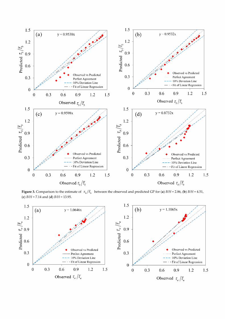
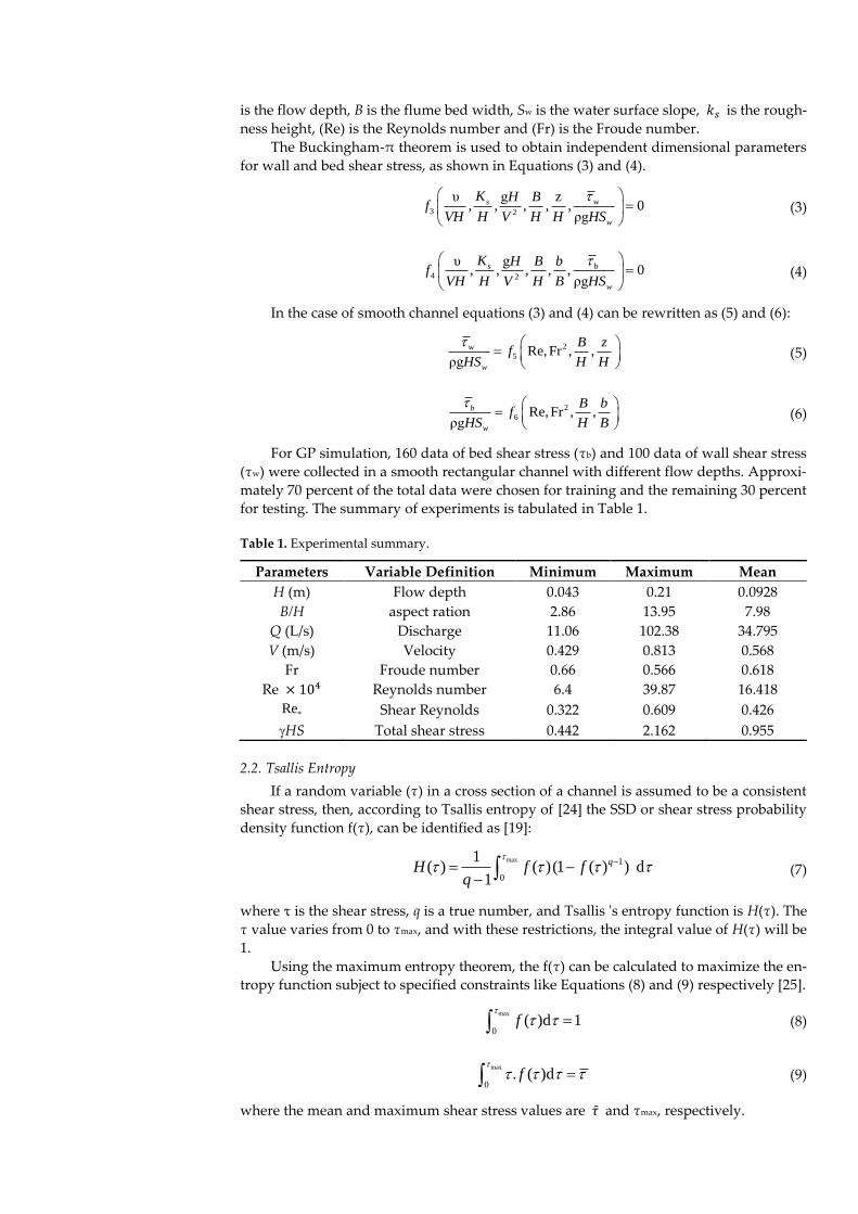
Figure 3. Comparison to the estimate of b b between the observed and predicted GP for (a) B/H = 2.86, (b) B/H = 4.51,

(c) B/H = 7.14 and (d) B/H = 13.95.

Figure 4. Comparison to the estimate of w w between the observed and predicted GP for (a) B/H = 2.86, (b) B/H = 4.51,

(c) B/H = 7.14 and (d) B/H = 13.95.

3.2. ANFIS Modeling

For this purpose, 70% of the experimental data was used for network training and

the remaining 30% was used for testing results. As input parameters to the model, the

parameters b/B and B/H for bed and z/H and B/H for the wall were presented. Figure 5

shows the performance of the ANFIS model to estimate the bed SSD (τb) and Figure 6

shows the performance of the ANFIS model to estimate the wall SSD (τw), 30% of the data,

which were not used in the training stage would be used to evaluate the performance of

the model. The results of statistical indexes for modeling shear stress with ANFIS are sum-

marized in Table 4. As well, the estimating bands of the four above parameters using to

determine the shear stress are shown in Figure 5. Skewness results obtained from statisti-

cal prediction dimensionless parameters.

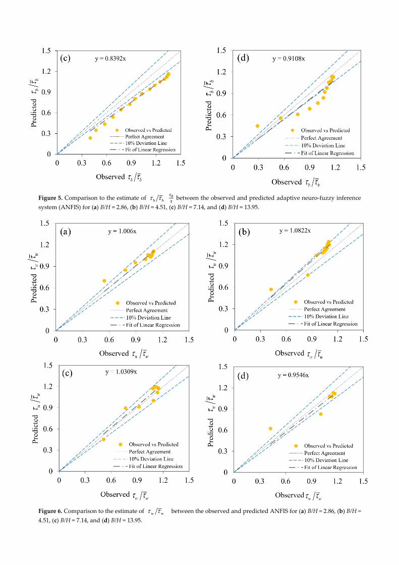
Figure 5. Comparison to the estimate of b b

𝜏𝑏

�̄� between the observed and predicted adaptive neuro-fuzzy inference

system (ANFIS) for (a) B/H = 2.86, (b) B/H = 4.51, (c) B/H = 7.14, and (d) B/H = 13.95.

Figure 6. Comparison to the estimate of w w between the observed and predicted ANFIS for (a) B/H = 2.86, (b) B/H =

4.51, (c) B/H = 7.14, and (d) B/H = 13.95.

Table 4. Performance metric of the ANFIS model to predict SSD.

B/H Bed Wall


2.86 0.2559 0.0991 0.1268 0.9279 0.0383 0.0314 0.0492 0.8026

4.51 0.1728 0.1240 0.1266 0.9744 0.0870 0.0959 0.1004 0.9033

7.14 0.2157 0.1699 0.1724 0.9871 0.0868 0.0634 0.0745 0.907

13.95 0.2278 0.1048 0.1271 0.8482 0.1792 0.0909 0.1145 0.7752

3.3. Comparison of the GP Model, Tsallis Entropy and ANFIS

The results of the best GP models and Tsallis entropy in shear stress prediction were

compared with the experimental results of Lashkar-Ara and Fatahi [8] in this section. Fig-

ures 7 and 8 show the experimental results and SSD predictions with different models in

a smooth rectangular channel for B/H equal to 2.85, 4.51, 7.14 and 13.95. Additionally, the

performance metric of the shear stress estimate by the Tsallis entropy model is shown in

Table 5. As shown in these statistics, all of the test evidence used to model the SSD using

the GP was is realized. For the training stage for modeling SSD in the rectangular channel

using the GP model, 70 percent of all data were used, and 30 percent of the data were used

for the testing process. As shown in Figure 7, for B/H= 2.86, 4.51, 7.14 and 13.95, the GP

model predicted the bed shear stress better than the Tsallis entropy model. In Figure 8c,d,

for B/H = 7.14 and 13.95, the GP model predicted wall shear stress better than the Tsallis

entropy model, but in Figure 8a,b, the Tsallis entropy was more accurately modeled to

predict wall shear stress than the GP model. Additionally, the GP model estimated bed

and wall shear stress better than the Tsallis entropy-based model at rising flow depth. It

is understandable that the channel architecture was challenging when a model expected

higher shear stress values. It is therefore not cost-effective to use the Tsallis entropy

method. When the GP model's observations were more accurate, it could be used to de-

sign stable channels more consistently. The GP model estimated the bed shear better than

the ANFIS model for B/H= 2.86, 4.51, 7.14 and 13.95. For B/H = 2.86, the ANFIS model

estimated the shear stress better than the GP model, but the GP model estimated the wall

shear stress better than the ANFIS model in B/H = 4.51, 7.14 and 13.95. The GP model

demonstrated superior efficiency to the Tsallis entropy-based model, while both models

neglected the influence of secondary flows. It can be inferred that the GP model of bed

and wall shear stress estimation was more sensitive than the Tsallis entropy method over-

estimated the values of bed shear stress and the GP model's outcomes were greater. The

bed shear stress values decreased at the middle of the channel (Figure 7), which varied

from other situations. From Figures 7 and 8, it can be shown that the GP model's fit line

was similar to the 45-degree line than the other ones, and with a higher value of NSE, its

predictions were more reliable. In predicting the position of maximal shear stress, both

the GP and Tsallis-entropy based models displayed the same pattern as the centerline of

the channel, which was consistent with the experimental outputs.

Figure 7. The dimensionless bed shear stress distribution for (a) B/H = 2.86, (b) B/H = 4.51, (c) B/H = 7.14 and (d) B/H =

13.95.

Figure 8. The dimensionless wall shear stress distribution for (a) B/H = 2.86, (b) B/H = 4.51, (c) B/H = 7.14 and (d) B/H =

13.95.

Table 5. Performance metric of Tsallis entropy to predict SSD.

B/H Bed Wall


2.86 1.252 0.0531 0.0706 0.9276 1.3145 0.0622 0.0797 0.7721

4.51 1.476 0.0522 0.0625 0.9425 1.3741 0.0749 0.0894 0.7632

7.14 1.538 0.0672 0.0685 0.9310 1.6254 0.0631 0.0738 0.8275

13.95 1.511 0.0643 0.0840 0.8426 1.2562 0.0893 0.1094 0.8398

4. Conclusions

The wall and bed shear stresses in a smooth rectangular channel measured experi-

mentally for different aspect ratios. Two soft computing models GP and ANFIS proposed

to estimate SSD in rectangular channel. In addition, the results of GP and ANFIS model

compared with a Tsallis based equation. Our research had some main findings as follows:

1. The effect of different input variable on the result was investigated to find the best

input combination.

2. In the present study B/H had the highest effect on the prediction power.

3. For bed shear stress predictions, the GP model, with an average RMSE of 0.0893 per-

formed better than the Tsallis entropy-based equation and ANFIS model with RMSE

of 0.0714 and 0.138 respectively.

4. To estimate the wall shear stress distribution the proposed ANFIS model, with an

average RMSE of 0.0846 outperformed the Tsallis entropy-based equation with an

RMSE of 0.0880 followed by the GP model with an RMSE of 0.0904.

Our finding suggests that the proposed GP algorithm could be used as a reliable and

cost-effective algorithm to enhance SSD prediction in rectangular channels.

Author Contributions: Supervision, B.L.-A.; Writing – original draft, B.L. -A. and N.K.; Writing –

review & editing, Z.S.K. and A.M. All authors have read and agreed to the published version of the

manuscript.

Funding: Not applicable.

Institutional Review Board Statement: Not applicable.

Informed Consent Statement: Not applicable.

Data Availability Statement: Not applicable.

Conflicts of Interest: The authors declare no conflict of interest.

References

1. Knight, D.W. Boundary shear in smooth and rough channels. J. Hydraul. Div. 1981, 107, 839–851.

2. Tominaga, A.; Nezu, I.; Ezaki, K.; Nakagawa, H. Three-dimensional turbulent structure in straight open channel flows. J. Hy-

draul. Res. 1989, 27, 149–173.

3. Seckin, G.; Seckin, N.; Yurtal, R. Boundary shear stress analysis in smooth rectangular channels. Can. J. Civ. Eng. 2006, 33, 336–

342, doi:10.1139/l05-110.

4. Khodashenas, S.R.; Paquier, A. A geometrical method for computing the distribution of boundary shear stress across irregular

straight open channels. J. Hydraul. Res. 1999, 37, 381–388.

5. Pope, N.D.; Widdows, J.; Brinsley, M.D. Estimation of bed shear stress using the turbulent kinetic energy approach-A compar-

ison of annular flume and field data. Cont. Shelf Res. 2006, 26, 959–970, doi:10.1016/j.csr.2006.02.010.

6. Knight, D.W.; Sterling, M. Boundary shear in circular pipes running partially full. J. Hydraul. Eng. 2000, 126, 263–275.

7. Park, J.H.; Do Kim, Y.; Park, Y.S.; Jo, J.A.; Kang, K. Direct measurement of bottom shear stress under high-velocity flow condi-

tions. Flow Meas. Instrum. 2016, 50, 121–127, doi:10.1016/j.flowmeasinst.2015.12.008.

8. Lashkar-Ara, B.; Fatahi, M. On the measurement of transverse shear stress in a rectangular open channel using an optimal

Preston tube. Sci. Iran. 2020, 27, 57–67, doi:10.24200/sci.2018.20209.

9. Berlamont, J.E.; Trouw, K.; Luyckx, G. Shear Stress Distribution in Partially Filled Pipes. J. Hydraul. Eng. 2003, 129, 697–705,

doi:10.1061/(ASCE)0733-9429(2003)129:9(697).

10. Sheikh Khozani, Z.; Wan Mohtar, W.H.M. Investigation of New Tsallis-Based Equation to Predict Shear Stress Distribution in

Circular and Trapezoidal Channels. Entropy 2019, 21, 1046, doi:10.3390/e21111046.

11. De Cacqueray, N.; Hargreaves, D.M.; Morvan, H.P. A computational study of shear stress in smooth rectangular channels. J.

Hydraul. Res. 2009, 47, 50–57, doi:10.3826/jhr.2009.3271.

12. Yang, J.Q.; Kerger, F.; Nepf, H.M. Estimation of the bed shear stress in vegetated and bare channels with smooth beds. Water

Resour. Res. 2015, 51, 3647–3663, doi:10.1002/2014WR016042.

13. Martinez-Vazquez, P.; Sharifi, S. Modelling boundary shear stress distribution in open channels using a face recognition tech-

nique. J. Hydroinform. 2017, 19, 157–172, doi:10.2166/hydro.2016.068.

14. Sterling, M.; Knight, D. An attempt at using the entropy approach to predict the transverse distribution of boundary shear stress

in open channel flow. Stoch. Environ. Res. Risk Assess. 2002, 16, 127–142.

15. Sheikh Khozani, Z.; Bonakdari, H. Formulating the shear stress distribution in circular open channels based on the Renyi en-

tropy. Phys. A Stat. Mech. Its Appl. 2018, 490, 114–126, doi:10.1016/j.physa.2017.08.023.

16. Sheikh Khozani, Z.; Bonakdari, H. A comparison of five different models in predicting the shear stress distribution in straight

compound channels. Sci. Iran. Trans. A Civ. Eng. 2016, 23, 2536–2545.

17. Sheikh Khozani, Z.; Hosseinjanzadeh, H.; Wan Mohtar, W.H.M. Shear force estimation in rough boundaries using SVR method.

Appl. Water Sci. 2019, doi:10.1007/s13201-019-1056-z.

18. Ardiçlioǧlu, M.; Sekçin, G.; Yurtal, R. Shear stress distributions along the cross section in smooth and rough open channel flows.

Kuwait J. Sci. Eng. 2006, 33, 155–168.

19. Bonakdari, H.; Tooshmalani, M.; Sheikh, Z. Predicting shear stress distribution in rectangular channels using entropy concept.

Int. J. Eng. Trans. A Basics 2015, 28, 360–367, doi:10.5829/idosi.ije.2015.28.03c.04.

20. Rankin, K.L.; Hires, R.I. Laboratory measurement of bottom shear stress on a movable bed. J. Geophys. Res. Ocean. 2000, 105,

17011–17019, doi:10.1029/2000jc900059.

21. Kisi, O.; Dailr, A.H.; Cimen, M.; Shiri, J. Suspended sediment modeling using genetic programming and soft computing tech-

niques. J. Hydrol. 2012, 450–451, 48–58, doi:10.1016/j.jhydrol.2012.05.031.

22. Sheikh Khozani, Z.; Bonakdari, H.; Ebtehaj, I. An analysis of shear stress distribution in circular channels with sediment depo-

sition based on Gene Expression Programming. Int. J. Sediment Res. 2017, 32, 575–584, doi:10.1016/J.IJSRC.2017.04.004.

23. Sheikh Khozani, Z.; Bonakdari, H.; Zaji, A.H. Estimating the shear stress distribution in circular channels based on the random-

ized neural network technique. Appl. Soft Comput. 2017, 58, 441–448, doi:10.1016/j.asoc.2017.05.024.

24. Tsallis, C. Possible generalization of Boltzmann-Gibbs statistics. J. Stat. Phys. 1988, 52, 479–487, doi:10.1007/BF01016429.

25. Jaynes, E.T. Information theory and statistical mechanics. II. Phys. Rev. 1957, 106, 620.

26. Singh, V.P.; Luo, H. Entropy Theory for Distribution of One-Dimensional Velocity in Open Channels. J. Hydrol. Eng. 2011, 16,

725–735, doi:10.1061/(ASCE)HE.1943-5584.0000363.

27. Jayawardena, A.W.; Muttil, N.; Fernando, T.M.K.G. Rainfall-runoff modelling using genetic programming. In Proceedings of

the International Congress on Modelling and Simulation: Advances and Applications for Management and Decision Making;

Melbourne, Australia, 12–15 December 2005; pp. 1841–1847.

28. Fatahi, M. and Lashkar-Ara, B., Estimating scour below inverted siphon structures using stochastic and soft computing ap-

proaches. Journal of AI and Data Mining, 2019, 5, 55-66.

29. Jang, J.S.R. ANFIS: Adaptive-Network-Based Fuzzy Inference System. IEEE Trans. Syst. Man Cybern. 1993, 23, 665–685,

doi:10.1109/21.256541.

30. Willmott, C.J. and Matsuura, K, Advantages of the mean absolute error (MAE) over the root mean square error (RMSE) in

assessing average model performance. Climate research, 2005, 30, 79-82.

31. McCuen, R.H., Knight, Z. and Cutter, A.G. Evaluation of the Nash–Sutcliffe efficiency index. Journal of hydrologic engineering,

2006, 11, 597-602.

Documents

Machine Learning versus Mathematical Model to Estimate the