Machine learning in policy evaluation: new tools

for causal inference

Noémi Kreif and Karla DiazOrdaz

Summary

While machine learning (ML) methods have received a lot of attention in recentyears, these methods are primarily for prediction. Empirical researchers conductingpolicy evaluations are, on the other hand, pre-occupied with causal problems, trying toanswer counterfactual questions: what would have happened in the absence of a policy?Because these counterfactuals can never be directly observed (described as the “funda-mental problem of causal inference”) prediction tools from the ML literature cannot bereadily used for causal inference. In the last decade, major innovations have taken placeincorporating supervised ML tools into estimators for causal parameters such as the av-erage treatment effect (ATE). This holds the promise of attenuating model misspecifica-tion issues, and increasing of transparency in model selection. One particularly maturestrand of the literature include approaches that incorporate supervised ML approachesin the estimation of the ATE of a binary treatment, under the unconfoundedness andpositivity assumptions (also known as exchangeability and overlap assumptions).

This article begins by reviewing popular supervised machine learning algorithms,including trees-based methods and the lasso, as well as ensembles, with a focus onthe Super Learner. Then, some specific uses of machine learning for treatment effectestimation are introduced and illustrated, namely (1) to create balance among treatedand control groups, (2) to estimate so-called nuisance models (e.g. the propensity score,or conditional expectations of the outcome) in semi-parametric estimators that targetcausal parameters (e.g. targeted maximum likelihood estimation or the double MLestimator), and (3) the use of machine learning for variable selection in situations witha high number of covariates.

Since there is no universal best estimator, whether parametric or data-adaptive, it isbest practice to incorporate a semi-automated approach than can select the models bestsupported by the observed data, thus attenuating the reliance on subjective choices.

Keywords— Machine learning, causal inference, treatment effects, health economics, program

evaluation, policy evaluation, doubly robust methods, matching

1

arX

iv:1

903.

0040

2v1

[st

at.M

L]

1 M

ar 2

019

1 Overview

Most scientific questions, such as those asked when evaluating policies, are causal in nature, even if

they are not specifically framed as such. Causal inference reasoning helps clarify the scientific

question, and define the corresponding causal estimand, i.e the quantity of interest, such as the

average treatment effect (ATE). It also makes clear the assumptions necessary to express the

estimand in terms of the observed data, known as identification. Once this is achieved, the focus

shifts to estimation and inference. While machine learning methods have received a lot of attention

in recent years, these methods are primarily geared for prediction. There are many excellent texts

covering machine learning focussed on prediction (Friedman et al., 2001; James et al., 2013), but

not dealing with causal problems. Recently, some authors within the Economics community have

started examining the usefulness of machine learning for the causal questions that are typically the

subject of applied econometric research (Varian, 2014; Kleinberg et al., 2015; Mullainathan and

Spiess, 2017; Athey, 2017b,a; Athey and Imbens, 2017).

In this Chapter, we contribute to this literature by providing an overview and an illustration of

machine learning methods for causal inference, with a view to answer typical causal questions in

policy evaluation, and show how these can be implemented with widely used statistical packages.

We draw on innovations form a wide range of quantitative social and health sciences, including

economics, biostatistics and political science.

We focus on methods to estimate the ATE of a binary treatment (or exposure), under “no

unobserved confounding assumptions” (see Section 2). The remainder of this article is as follows.

First, we introduce the notation and the assumptions for the identification of causal effects. Then

we outline our illustrative treatment effect estimation problem, an impact evaluation of a social

health insurance program in Indonesia. Next, we provide a brief introduction to supervised

machine learning methods. In the following sections, we review methods for estimating the ATE.

2

These can be roughly categorised into three main types: methods that aim to balance covariate

distributions (propensity scores (PS) and other matching methods), methods that fit outcome

regressions to “impute” potential outcomes and estimate causal effects, and the so called “double

robust” methods that combine these. We also discuss the use of machine learning for variable

selection, a challenge increasingly important with “Big data”, especially with a large number of

variables. In the last section we provide a brief overview of developments for other settings and a

discussion.

2 Estimands and assumptions for identification

2.1 Notation and assumptions

Let A be an indicator variable for treatment, and Y be the outcome of interest. Denote by Y ai the

potential outcome that would manifest if the i-th subject were exposed to level a of the treatment,

with a ∈ {0, 1}. The observed outcome can then be written as Yi = Y 0i (1−Ai) + Y 1

i Ai (Rubin,

1978).

Throughout, we assume the Stable Unit Treatment Value Assumption (SUTVA) holds, which

comprises no interference, i.e. the potential outcomes of the i-th individual are unrelated to the

treatment status of all other individuals, and consistency, i.e. for all individuals i = 1, . . . , N , if

Ai = a then Y ai = Yi, for all a (Robins et al., 2000; VanderWeele, 2009; Cole and Frangakis, 2009;

Pearl, 2010).

Denote the observed data of each individual by Oi = (Xi, Ai, Yi), where Xi is a vector of

confounding variables, that is factors that influence simultaneously the potential outcomes and

treatment. We assume that the data are an independent identically distributed sample of size N .

Individual level causal effects are defined as the difference between these “potential outcomes”.

3

Researchers are often interested in the average of these individual causal effects over some

population. A widely considered casual estimand is the ATE, defined as ψ = E[Y 1i − Y 0

i ]. Further

estimands include the average taken over the treated subjects (the average treatment effect on the

treated, ATT) or the conditional average treatment effect (CATE), which takes the expectation

over individuals with certain observed characteristics. Here we focus on the ATE.

Since the potential outcomes can never be simultaneously directly observed, these estimands

cannot be expressed in terms of observed data, or identified, without further assumptions. A

commonly invoked assumption which we will make throughout is ignorability or unconfoundedness

of the treatment assignment, (also known as conditional exchangeability). This assumption requires

that the potential outcomes are independent of treatment, conditional on the observed covariates,

Ai ⊥ (Y 0i , Y

1i )|Xi = x. (1)

The plausibility of this assumption needs to be carefully argued in each case, ideally with careful

data collection and based on subject matter knowledge about the variables that may be associated

with the outcome as well as influencing the treatment, as it cannot be tested using the observed

data (Rubin, 2005).

The second necessary assumption is the positivity of the treatment assignment (also referred as

“overlap”):

0 < P (Ai = 1|Xi = x) < 1, (2)

implying that for any combination of covariates, there is a nonzero probability of receiving both

the treatment and control states.

Using the unconfoundedness and the positivity assumptions, the conditional mean of the potential

outcomes corresponds with the conditional mean of the observed outcomes,

4

E[Y 1i |Xi, Ai = 1] = E[Yi|Xi, Ai = 1] and E[Y 0

i |Xi, Ai = 0] = E[Yi|Xi, Ai = 0], and the ATE can

be identified by:

ψ = E[Yi|Xi, Ai = 1]− E[Yi|Xi, Ai = 0]. (3)

3 Illustrative example: the impact of health insurance

on assisted birth in Indonesia

We illustrate the methods by applying them each in turn to an impact evaluation of a national

health insurance programme in Indonesia (more details in Kreif et al. (2018)). The dataset consists

of births between 2002 and 2014, extracted from the Indonesian Family Life Survey (IFLS). The

policy of interest, i.e. the treatment, is “being covered by the health insurance offered for those in

formal employment and their families” (contributory health insurance). We are interested in the

ATE of such health insurance on the probability of the birth being assisted by a health care

professional (physician or midwife). We construct a list of observed covariates including the

mother’s characteristics, (age, education, wealth in quintiles) and household’s characteristics

(social assistance, experienced a natural disaster, rurality, availability of health services: a village

midwife, birth clinic, hospital).

We expect that the variables describing socioeconomic status may be particularly important,

because those with contributory insurance tend to work in the formal sector, and have higher

education than those uninsured, and these characteristics would make a mother more likely to use

health services even in the absence of health insurance. Similarly, the availability of health services

is expected to be an important confounder, as those who have health insurance may live in areas

where it is easier to access health care, with or without health insurance.

The final dataset reflects typical characteristics of survey data: the majority of variables are

5

binary, with two variables categorical and one continuous (altogether 34 variables). Due to the

nature of the survey, for around one third of women we could not measure confounder information

from the past, but had to impute it with information from the time of the survey. Two binary

variables indicate imputed observations.

For simplicity, any records with any other missing data have been list-wise deleted. This approach

provides unbiased estimates of the ATE as long as missingness does not depend on both the

treatment and the outcome (Bartlett et al., 2015). The resulting complete-case dataset consists of

10985 births, of whcih 1181 are in the treated group, as the mother had health insurance in the

year of the child’s birth, while 8574 babies had their birth assisted by a health professional.

4 Introduction to machine learning for causal inference

4.1 Supervised machine learning

The type of machine learning tools most useful for causal inference are those labelled as

“supervised machine learning”. These tools, similarly to regression, can summarise linear and

non-linear relationships in the data and can predict some Y variable given new values of covariates

(A,X) (Varian, 2014). A “good” prediction is defined in relation to a loss function, for example the

mean sum of squared errors. A commonly used measure of this is the test mean squared error (test

MSE), defined as the average square prediction error among observations not previously seen. This

quantity differs from the usual MSE calculated among observations that were used to fit the

model. In the absence of a very large dataset that can be used to directly estimate the test MSE,

it can be estimated by holding out a subset of the observation from the model fitting process, using

the so-called “V-fold cross-validation” procedure (see e.g. Zhang (1993)). When performing V -fold

cross-validation, the researcher randomly divides the set of observations into V groups (folds). The

6

first group is withheld from the fitting process, and thus referred to as the test data. The algorithm

is then fitted using the data in the remaining V − 1 folds, called the training data. Finally, the

MSE is calculated using the test data, thus evaluating the performance of the algorithm. This

process is repeated for each fold, resulting in V estimates of the test MSE, which are then averaged

to obtain the so-called cross-validated MSE. In principle, it is possible to perform cross-validation

with just one split of the sample, though results are highly dependent on the sample split. Thus,

typically, V = 5 or V = 10 is used in practice.

The ultimate goal of machine learning algorithms is to get good out-of-sample predictions

minimising the test MSE (Varian, 2014), typically achieved by a combination of flexibility and

simplicity, often described as the “bias-variance trade off”. The formula for the MSE shows why

minimising it achieves this: MSE(θ) = Var(θ) + Bias(θ, θ)2. For example, a nonlinear model with

many higher order terms is more likely to fit the data better than a simpler model, however it is

unlikely that it will fit a new dataset similarly well, often referred to as “overfitting”.

Regularisation is a general approach that aims to achieve balance between flexibility and

complexity, by penalising more complex models. With less regularisation, one does a better job at

approximating the within-sample variation, but for this very reason, the out-of-sample fit will

typically get worse, increasing the bias. The key question is choosing the level of regularisation:

how to tune the algorithm so that it does not over-smooth or overfit.

In the context of selecting regularisation parameters, cross-validation can be used to perform

so-called empirical tuning to find the optimal level of complexity, where complexity is often

indexed by the tuning parameters. The potential range of tuning parameters is divided into a grid

(e.g. 10 possible values), and V fold cross validation process is performed for each parameter value,

enabling the researcher to choose the value of the tuning parameter with the lowest test MSE.

Finally, the algorithm with the selected tuning parameter is re-fitted using all observations.

7

4.2 Prediction vs. causal inference

Machine learning is naturally suited to prediction problems, which have been traditionally treated

as distinct from causal questions (Mullainathan and Spiess, 2017). It may be tempting to interpret

causally the output of the machine learning predictions, however making inferences from machine

learning models is complicated by (1) the lack of interpretable coefficients for some of the

algorithms, and (2) the lack of standard errors (Athey, 2017a). Moreover, for certain

“regression-like” algorithms (e.g. Lasso), selecting the best model using cross validation, and then

doing inference for the model parameters, ignoring the selection process, though common in

practice, should be avoided as it leads to potential biases stemming from the shrunk coefficients,

and underestimation of the true variance in the parameter estimates (Mullainathan and Spiess,

2017).

The causal inference literature (see e.g. Kennedy (2016); Van der Laan and Rose (2011); Petersen

(2014)) stresses the importance of first defining the causal estimand of interest (also referred to as

‘’target parameter”), and then carefully thinking about the necessary assumptions for

identification. Once the causal estimand has been mapped to an estimator (a functional of the

observed data), via the identification assumptions, the problem becomes an estimation exercise. In

practice many estimators involve models for parameters (e.g. conditional distributions, means),

which are not of interest per se, but are necessary to estimate the target parameter, these are called

nuisance models. Nuisance models estimation can be thought of as prediction problem for which

machine learning can be used. Examples include the estimation of propensity scores, or outcome

regressions that can later be used to predict potential outcomes (see Section 7). So while most

machine learning methods cannot be readily used to infer causal effects, they can help the process.

A potential key advantage of using machine learning for the nuisance models is that it fits and

compares many alternative algorithms, by for example, using cross validation (while

8

cross-validation can be used to select among parametric models as well). Selecting models based

on a well defined loss functions (e.g. the cross-validated MSE) can, beyond improving model fit,

benefit the overall transparency of the research process (Athey, 2017b). This is in contrasts with

how model selection is usually viewed in Economics, where model is chosen based on theory and

estimated only once.

This has led to many researchers using machine-learning for the estimation of the nuisance

parameters of standard estimators (e.g., outcome regression, inverse probability weighting by the

propensity score, see e.g. Lee et al. (2010); Westreich et al. (2010)). However, the behavior of these

estimators is can be poor, resulting in slower convergence rates and confidence intervals which are

difficult to construct (van der Vaart, 2014). In addition, the resulting estimators are irregular and

the nonparametric bootstrap is in general not valid (Bickel et al., 1997).

An increasingly popular strategy to avoid these biases and have valid inference is to use the

so-called doubly robust estimators (combining nuisance models for the outcome regressions and the

propensity score) which we review in Section 5.6. This is because DR estimators can converge at

fast rates (√N) to the true parameter, and are therefore consistent asymptotically normal, even

when the nuisance models have been estimated via machine learning.

In the following sections, we briefly describe the machine learning approaches that have been most

widely used for nuisance model prediction in causal inference, either because of their similarity to

traditional regression approaches, their easy implementation due to the availability of statistical

packages, their superior performance in prediction, or a combination of these.

4.3 Lasso

LASSO (Least Absolute Shrinkage and Selection Operator) is a penalised linear (or generalised

linear) regression algorithm, fitting the model including all d predictors. It aims to find the set of

9

coefficients that minimise the sum-of-squares loss function, but subject to a constraint on the sum

of absolute values (or `1 norm) of coefficients being equal to a constant c often referred to as

budget, i.e.∑d

j=1 ‖βj‖1 = c. This results in a (generalised) linear regression in which only a small

number of covariates have nonzero coefficient: this absolute-value regulariser induces a sparse

coefficient vector. The nonzero coefficient estimates are also shrunk towards zero. This significantly

reduces their variance at the “price” of increasing the bias. An equivalent formulation of the lasso is

minβ∈Rd

{‖y −Xβ‖2 + λ‖β‖1

}, (4)

with the penalty λ being the tuning parameter.

As λ increases, the flexibility of the lasso regression fit decreases, leading to decreased variance but

increased bias. Beyond a certain point however, the decrease in variance due to increasing λ slows,

and the shrinkage on the coefficients causes them to be significantly underestimated, resulting in a

large increase in the bias. Thus the choice of λ is critical. This is usually done by cross-validation,

implemented by several R packages, e.g. glmnet and caret.

Because the lasso results in some of the coefficients being exactly zero when the penalty λ is

sufficiently large, it essentially performs variable selection. The variable selection however is driven

by the tuning parameter, and it can happen that some variables are selected in some of the CV

partitions, but may be unused in another. This problem is common when the variables are

correlated with each other, and they explain very similar “portions” of the outcome variability. A

practical implication of this is that the researcher should remove from the set of potential variables

those that are irrelevant, in the sense that they are very correlated to a combination of other, more

relevant ones.

Another problem is inference after model selection, with some results (Leeb and Benedikt, 2008)

10

showing its is not possible to obtain (uniform) model selection consistency. As we demonstrate in

Section 6 some uses of lasso enable consistent estimation post-variable selection.

4.4 Tree based methods

4.4.1 Regression trees

Tree based methods, also known as classification and regression trees or “CARTs”, have a similar

logic to decision trees familiar to economists, but here the “decision” is a choice about how to

classify the observation. The goal is to construct (or “grow”) a decision tree that leads to good

out-of-sample predictions. They can be used for classification with binary or multicategory

outcomes (“classification trees”) or with continuous outcomes (“regression trees”). A regression tree

uses a recursive algorithm to estimate a function describing the relationship between a multivariate

set of independent variables and a single dependent variable, such as treatment assignment.

Trees tend to work well for settings with nonlinearities and interactions in the outcome-covariate

relationship. In these cases, they can improve upon traditional classification algorithms such

logistic regression. In order to avoid overfitting, trees are pruned by applying tuning parameters

that penalise complexity (the number of leaves). A major challenge with tree methods is that they

are sensitive to the initial split of the data, leading to high variance. Hence, single trees are rarely

used in practice, but instead ensembles - algorithms that stack or add together different algorithms

- of trees are used, such as random forest or boosted CARTs.

4.4.2 Random forests

Random forests are constructed using bootsrapped samples of the data, and growing a tree where

only a (random) subset of covariates is used for creating the splits (and thus the leaves). These

trees are then averaged, which leads to a reduction in variance. The tuning parameters, which can

11

be set or selected using cross validation, include the number of trees, depth of each tree, and the

number of covariates to be randomly selected (usually recommended to be approximately√d

where d is the number of available independent variables). Popular implementations include the R

packages caret and ranger.

4.4.3 Boosting

Boosting generates a sequence of trees where the first tree’s residuals are used as outcomes for the

construction of the next tree. Generalised boosted models add together many simple functions to

estimate a smooth function of a large number of covariates. Each individual simple function lacks

smoothness and is a poor approximation to the function of interest, but added together they can

approximate a smooth function just like a sequence of line segments can approximate a smooth

curve. In the implementation in the R package gbm (McCaffrey et al., 2004), each simple function

is a regression tree with limited depth. Another popular package is xgboost.

4.4.4 Bayesian Additive Regression Trees

Bayesian Additive Regression Trees (BARTs) can be distinguished from other tree based

ensembling algorithms due to its underlying probability model (Kapelner and Bleich, 2013). As a

Bayesian model, BART consists of a set of priors for the structure and the leaf parameters and a

likelihood for data in the terminal nodes. The aim of the priors is to provide regularisation,

preventing any single regression tree from dominating the total fit. To do this, BARTs employ

so-called “Bayesian backfitting” where the j-th tree is fit iteratively, holding all other m− 1 trees

constant by exposing only the residual response that remains unfitted. Over many MCMC

iterations, trees evolve to capture the fit left currently unexplained (Kapelner and Bleich, 2013).

BART is described as particularly well-suited to detecting interactions and discontinuities, and

12

typically requires little parameter tuning (Hahn et al., 2017). There is ample evidence on BART’s

good performance in predictions and even in causal inference (Hill, 2011; Dorie et al., 2017), and is

implemented in several R packages (bartMachine, dbarts). Despite its excellent performance in

practice, there are limited theoretical results about BARTs.

4.5 Super Learner ensembling

Varian (2014) highlights the importance of recognising uncertainty due to the model selection

process, and the potential role ensembling can play in combining several models to create one that

outperforms single models. Here we focus on the Super Learner (SL) (van der Laan and Dudoit,

2003), a machine learning algorithm that uses cross validation to find the optimal weighted convex

combination of multiple candidate prediction algorithms. The algorithms pre-specified by the

analyst form the library, and can include parametric and machine learning approaches. The Super

Learner has the oracle property, i.e. it produces predictions that are at least as good as those of

the best algorithm included in the library (see van der Laan et al. (2007); Van der Laan and Rose

(2011) for details).

Beyond its use for prediction (Polley and van der Laan, 2010; Rose, 2013), it has been used for PS

and outcome model estimation (see for example, (Eliseeva et al., 2013; van der Laan and Luedtke,

2014; Gruber et al., 2015)), and has been shown to reduce bias from model misspecification (Porter

et al., 2011; Kreif et al., 2016; Pirracchio et al., 2015). Implementations of the Super Learner

include the SuperLearner, h2oEnsembleR and the subsemble R packages, the latter two with

increased computational speed to suit large datasets.

13

5 Machine learning methods to create balance between

covariate distributions

5.1 Propensity score methods

The propensity score (PS) (Rosenbaum and Rubin, 1983) defined as the conditional probability of

treatment A given observed covariates, i.e. p(xi) = P (Ai = 1|Xi = xi), is referred to as a

“balancing score”, due to its property of balancing the distributions of observed confounders

amongst the treatment and control groups. The propensity score has been widely used to control

for confounding, either for subclassification (Rosenbaum and Rubin, 1984), as a metric to establish

matched pairs in nearest neighbor matching (Rubin and Thomas, 1996; Abadie and Imbens, 2016),

and for reweighting, using inverse probability of treatment weights (Hirano et al., 2003). The latter

two approaches have been demonstrated to have the best performance (Lunceford and Davidian,

2004; Austin, 2009).

The PS matching estimator constructs the missing potential outcome using the observed outcome

of the closest observation(s) from the other group, and calculates the ATE as a simple mean

difference between these predicted potential outcomes (Abadie and Imbens, 2006, 2011, 2016).

The inverse probability of treatment weighting (IPTW) estimator for the ATE is simply a weighted

mean difference between the observed outcomes of the treatment and control groups, where the

weights wi are constructed from the estimated propensity score as

wi =Ai

p(Xi)+

(1−Ai)1− p(Xi)

. (5)

With a correctly specified p(X), ψIPTW is consistent and efficient (Hirano et al., 2003). The

14

IPTW estimator can be expressed as

ψIPTW =1

N

N∑i=1

AiYip(Xi)

− (1−Ai)Yi1− p(Xi)

. (6)

Obtaining SEs for IPTW estimators can be done by the Delta method assuming the PS is known,

or using robust covariance matrix, so-called sandwich estimator to acknowledge that the PS was

estimated, or by bootstrapping. IPTW estimators are sensitive to large weights.

The validity of these methods depends on correctly specifying the PS model. In empirical work,

typically probit or logistic regression models are used without interactions or higher order terms.

However, the assumptions necessary for these to be correctly specified, for example the linearity of

the relationship between covariates and probability of treatment in the logit scale, are rarely

assessed (Westreich et al., 2010). More flexible modelling approaches, such as series regression

estimation (Hirano et al., 2003), and machine learning methods, including decision trees, neural

networks and linear classifiers (Westreich et al., 2010), generalised boosting methods (McCaffrey

et al., 2004; Westreich et al., 2010; Lee et al., 2010; Wyss et al., 2014) or the Super Learner

(Pirracchio et al., 2012) have been proposed to improve the specification of the PS. However, even

such methods may have poor properties, if their loss function targets measures of model fit (e.g.

log likelihood, area under the curve) instead of balancing covariates that are important to reduce

bias (Westreich et al., 2011). Imai and Ratkovic (2014) proposed a score that explicitly balances

the covariates, exploiting moment conditions that capture the desired mean independence between

the treatment variable and the covariates that the balancing aims to achieve. A machine learning

method for estimating propensity scores that aims to maximise balance is the boosted CART

approach (McCaffrey et al., 2004; Lee et al., 2010), implemented as the TWANG R package. This

approach minimises a chosen loss function, based on covariate balance achieved in the IPTW

15

weighted data, by iteratively forming a collection of simple regression tree models and adding them

together to estimate the propensity score. It models directly the log-odds of treatment rather than

the propensity scores, to simplify computations. The algorithm can be specified to stop when the

best balance is achieved. A recommended stopping rule is the average standardised absolute mean

difference (ASAM) in the covariates. A balance metric, the number of iterations, depth of

interactions and shrinkage parameters need to be specified. The boosted CART approach to

estimating PS has been demonstrated to improve balance and reduce bias in the estimated ATE

(Lee et al., 2010; Setoguchi et al., 2008) and has been extended to settings with continuous

treatments (Zhu et al., 2015).

5.2 Methods aiming to directly create balanced samples

There is an extensive literature on methods that aim to create matched samples that are

automatically balanced on the covariates, instead of estimating and matching on a PS. An

extension of Mahalanobis distance matching, the “Genetic Matching” algorithm (Diamond and

Sekhon, 2013) searches a large space of potential matched treatment and control groups to

minimise loss functions based on tests statistics describing covariate imbalance (e.g.

Kolmogorov-Smirnov tests). The accompanying Matching R package (Sekhon, 2011; Mebane Jr

et al., 2011) has a wide range of matching methods (including propensity score), matching options

(e.g. with or without replacement, 1:1 or 1:m matching), estimands (ATE vs ATT) and balance

statistics. The “Genetic” component of the matching algorithm chooses weights to give relative

importance to the matching covariates to optimise the specified loss function. The algorithm

proposes batches of weights, “a generation”, and moves towards the batch of weights which

maximise overall balance. Each generation is then used iteratively to produce a subsequent

generation with better candidate weights. The “population size”, i.e. the size of each generation is

16

the tuning parameter to be specified by the user.

Similar approaches to creating optimal matched samples, with a different algorithmic solution are

offered by Zubizarreta (2012) and Hainmueller (2012). Both approaches use integer programming

optimisation algorithms to construct comparison groups given balance constraints (maximum

allowed imbalance) specified by the user, in the former case by one-to-many matching, in the latter

case by constructing optimal weights.

5.3 Demonstration of balancing methods using the birth dataset

We estimate a range of PS: first, using a main terms logistic regression to estimate the conditional

probability of being enrolled in health insurance, followed by two data-adaptive propensity scores.

We include all covariates in the prediction algorithms, without prior covariate selection. The first

is a boosted CART, with 5000 trees, of a maximum depth of 2 interactions, and shrinkage of 0.005.

The loss function used is “average standardised difference”.

Second, we use the Super Learner with a library containing a range of increasingly data-adaptive

prediction algorithms:

• logistic regression with and without all pair-wise interaction

• generalised additive models with 2, 3 and 4 degrees of freedom,

• random forests - including 4 random forest learners varying the number of trees (500, 2000),

and the number of covariates to split on (5 and 8), implemented in the ranger R package),

• boosting - using the R package xgboost, with varying number of trees (100 and 1000),

shrinkage (0.001 and 0.1) and maximum tree depth (1 and 4)).

• a BART prediction algorithm using 200 regression trees with the tuning parameters set to

default implementation in the dbarts R package.

17

We use 10-fold cross-validation and the mean sum of squares loss function. For the purposes of

comparison, we have also implemented two 1:1 matching estimators with replacement, for the ATE

parameter. First, we created a matched dataset based on the boosted CART propensity score,

implemented without calipers. Second, we implemented the Genetic Matching algorithm, using a

population size of 500, and a loss function that aims to minimise the largest p-values from paired

t-test. We have re-assessed the balance for the pair matched data. Throughout, we evaluate

balance based on standardised mean differences, a metric that is comparable across weighting and

matching methods (Austin, 2009). We calculate the ATE using IPTW and matching. The SEs for

the IPTW are “sandwich” SEs while for the matching estimators the Abadie-Imbens formula is

used Abadie and Imbens (2006) that accounts for matching with replacement.

Figure 1 can be inspected to assess the relative performance of the candidate algorithms included

in the SL. It displays the cross-validated estimates of the loss function (MSE) after an additional

layer of cross-validation, so that the out-of sample performance of each individual algorithm and

the convex combination of these algorithms (Super Learner) can be compared. The “Discrete SL”

is defined as an algorithm that gives the best candidate the weight of 1. We see that the convex

Super Learner performs best. Table 1 show the coefficients attributed to the different candidate

algorithms in the final prediction algorithm that was used to estimate the PS.

Table 1: Non-zero weights corresponding to the algorithms in the convex Super Learner, forestimating propensity scores.

Algorithm’s weight in ensembleRandom Forest (500 trees, 5 variables) 0.18Random Forest (2000 trees, 5 variables) 0.36

Generalised additive models degree 3 0.46GLM with all 2-way interactions 0.01

For each propensity score and matching approach, we compare balance on the covariates in the

data (reweighted by IPTW weights or by frequency weights from the matching, respectively).

18

Figure 1: Estimated Mean Squared Error loss from candidate algorithms of the SuperLearner

Algorithms labelled by Rg are variations of random forests, algorithmslabelled by xgb are variations of the boosting algorithm. Algorithmslabelled with SL are implemented in the SuperLearner R package.

Figure 2 displays the absolute standardised differences (ASD) for all the covariates, starting from

the variables that were least imbalanced in the unweighted data, moving towards the more

imbalanced. Generally, all weighting approaches tend to improve balance compared to the

unweighted data, except for variables that were well balanced (ASD < 0.05) to begin with. Using

the rule of thumb of 0.1 as a metric of significant imbalance, we find that TWANG, when used for

weighting, achieves acceptable balance on all covariates, except for the binary variable indicating

having at least secondary education. Based on the more stringent criterion of ASD < 0.05,

however, TWANG leaves several covariates imbalanced, including the indicator of rural

community, the availability of health center, the availability of birth clinic, and whether the

mother can write in Indonesian. When used for pair matching, the boosted CART based

propensity score leaves high imbalances. This is expected as the balance metric in the loss function

used the weighted, and not the matched data. The SL-based propensity score results in the largest

imbalance, again reflecting that the loss function was set to maximimise the cross-validated MSE

19

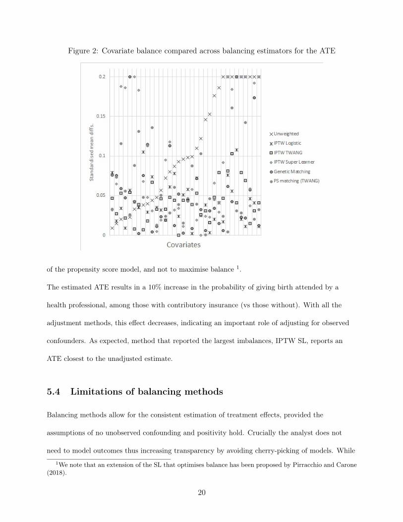
Figure 2: Covariate balance compared across balancing estimators for the ATE

of the propensity score model, and not to maximise balance 1.

The estimated ATE results in a 10% increase in the probability of giving birth attended by a

health professional, among those with contributory insurance (vs those without). With all the

adjustment methods, this effect decreases, indicating an important role of adjusting for observed

confounders. As expected, method that reported the largest imbalances, IPTW SL, reports an

ATE closest to the unadjusted estimate.

5.4 Limitations of balancing methods

Balancing methods allow for the consistent estimation of treatment effects, provided the

assumptions of no unobserved confounding and positivity hold. Crucially the analyst does not

need to model outcomes thus increasing transparency by avoiding cherry-picking of models. While

1We note that an extension of the SL that optimises balance has been proposed by Pirracchio and Carone(2018).

20

Table 2: ATEs and 95 % CIs estimated using IPTW and matching methods

ATE 95 % CI L 95 % CI UUnadjusted (naive) 0.13 0.11 0.16

IPTW logistic 0.06 0.02 0.11IPTW TWANG 0.08 0.04 0.12

IPTW SL 0.11 0.09 0.13PS matching TWANG 0.08 0.04 0.12

Genetic Matching 0.06 0.03 0.09

machine learning can help by making the choices of the PS model or a distance metric

data-adaptive, subjective choices remain. For example, the loss function needs to be specified, and

if the loss function is based on balance, also the choice of balance metric. For example, the ASM

chosen for demonstration purposes creates a metric of average imbalance for the means. This

ignores two potential complexities. First, imbalances in higher moments of the distribution are not

taken into account by this metric. While Kolmogorov-Smirnov tests statistics can take into

account imbalance in the entire covariate distribution (Stuart, 2010; Diamond and Sekhon, 2013),

and can be selected to enter the loss function for both the boosted CART and the Genetic

Matching algorithms, there is a further issue remaining: how should the researcher trade-off

imbalance across covariates? With a large number of covariates, balancing one variable may

decrease balance on an other covariate. Moreover, it is unclear how univariate balance measures

should be summarised. The default of the TWANG package is to look at average covariate

balance, while the Genetic Matching algorithm, as default, prioritises covariate balance on the

variable that is the most imbalanced. This, however may not prioritise variables that are relatively

strong predictors of the outcome, and any remaining imbalance would translate into a larger bias.

Hence, there is an increasing consensus that exploiting information from the outcome regression

generally improves on the properties of balance-based estimators (Kang et al., 2007; Abadie and

Imbens, 2011). ML methods to estimate the nuisance models for the outcome can provide

reassurance against subjectively selecting outcome models that provide the most favourable

21

treatment effect estimate. We review these methods in the following section.

5.5 Machine learning methods for the outcome model

Recall that under the unconfoundedness and positivity assumptions, the ATE can be identified by

E[Y |A = 1,X]− E[Y |A = 0,X], reducing the problem to one of estimation of these conditional

expectations (Imbens and Wooldridge, 2009; Hill, 2011). Denoting the true conditional expectation

function for the observed outcome as µ(A,X) = E[Y |A,X], the regression estimator for the ATE

can be obtained as

ψreg =1

N

N∑i=1

{µ(A = 1,Xi)− µ(A = 0,Xi)

}, (7)

where µ(A = a,X = x) can interpreted as the predicted potential outcome for level a of the

treatment among individuals with covariates X = x, and can be estimated by for example a

regression E[Y |A = a,X = x] = η0(x) + β1a, with η0(x) the nuisance function and β1 the

parameter of interest for level a of the treatment. Under correct specification of the models for

µ(A,X), the outcome regression estimator is consistent (Bang and Robins, 2005), but it is prone to

extrapolation.

The problem can now be viewed as a prediction problem, making it appealing to use ML to obtain

good predictions for µ(A,X). Indeed, some methods do this: BARTs have been successfully used

to obtain ATEs (Hill, 2011; Hahn et al., 2017). Austin (2012) demonstrates the use of a wide range

of tree-based machine learning techniques to obtain regression estimators for the ATE.

However, there are three reasons why ML is generally not recommended for outcome regression.

First, the asympototic properties of such estimators are unknown. Typically, the convergence of

the resulting regression estimator for the causal effect will be slower than√N when using ML fits.

A related problem is the so-called “regularisation bias” (Chernozhukov et al., 2017; Athey et al.,

22

2018). Data-adaptive methods use regularisation to achieve optimal bias-variance trade-off, which

shrinks the estimates towards zero, introducing bias (Mullainathan and Spiess, 2017), especially if

the shrunk coefficients correspond to variable which are strong confounders (Athey et al., 2018).

This problem increases as the number of parameters compared to sample size grows. Third, it is

difficult to conduct inference for causal parameters, as in general there is no way of constructing

valid confidence intervals, and the non-parametric bootstrap is not generally valid (Bickel et al.,

1997).

This motivates going beyond single nuisance model ML plug-in estimators, and using

double-robust estimators with ML nuisance model fits, reviewed in the next section (Farrell, 2015;

Chernozhukov et al., 2017; Athey et al., 2018; Seaman and Vansteelandt, 2018).

5.6 Double-robust estimation with machine learning

Methods that combine the strengths of outcome regression modelling with the balancing properties

of the propensity score have been advocated for long. The intuition is that using propensity score

matching or weighting as a “pre-processing” step can be followed by regression adjustment to

control further for any residual confounding (Rubin and Thomas, 2000; Abadie and Imbens, 2006;

Imbens and Wooldridge, 2009; Stuart, 2010; Abadie and Imbens, 2011). While these methods have

performed well in simulations (Kreif et al., 2013; Busso et al., 2014; Kreif et al., 2016), their

asymptotic properties are not well understood.

A formal approach to combining outcome and treatment modelling was originally developed to

improve the efficiency of IPTW estimators (Robins et al., 1995). Double-robust (DR) estimators

use two nuisance models, and have the special property that they are consistent as long as at least

one of the two nuisance models is correctly specified. In addition, some DR estimators are shown

to be semi-parametrically efficient, if both components are correctly specified (Robins et al., 2007).

23

A simple DR method is the augmented inverse probability weighting ( AIPTW) estimator (Robins

et al., 1994). The AIPTW can be written as ψAIPTW = ψAIPTW (1)− ψAIPTW (0), where

ψAIPTW (a) =1

N

N∑i=1

(YiI(Ai = a)

p(Xi)− I(Ai = a)− p(Xi)

p(Xi)µ(Xi, Ai)

), (8)

where µ(A,X) = E[Y |A,X], as before.

The variance of DR estimators is based on the variance of their influence function. Let ψ be an

estimator of a scalar parameter ψ0, satisfying

√N(ψ − ψ0) =

√N−1

N∑i=1

φ(Oi) + o(1), (9)

where o(1) denotes a term that converges in probability to 0, and where E[φ(O)] = 0 and

0 < E[φ(O)2] <∞, i.e. φ(O) has zero mean and finite variance. Then φ(O) is the influence

function (IF) of ψ.

By the central limit theorem, the estimator ψ is asymptotically normal with asymptotic variance

N−1 times the variance of its influence function using this to construct normal-based confidence

intervals.

A consequence of this convergence behaviour is that good asymptotic properties of DR estimators

can be achieved even when the convergence rates of the nuisance models are slower than the

conventional√N , as the DR estimator ψ can still converge at a fast

√N rate, as long as the

product of the nuisance models convergence rates is faster than√N (under regularity conditions,

and empirical process conditions (e.g. Donsker class which can be avoided via sample splitting

(Bickel and Kwon, 2001; van der Laan and Robins, 2003; Chernozhukov et al., 2017), described

later).

This discovery allows for the use of flexible machine learning-based estimation of the nuisance

24

functions, leading to an increased applicability of DR estimators, which were previously criticised,

given that most likely both nuisance models are misspecified (Kang et al., 2007). Concerns about

the sensitivity to extreme propensity score weights remain (Petersen et al., 2012).

To improve on AIPTW estimators, Van Der Laan and Rubin (2006) introduced targeted minimum

loss based estimation (TMLE), a class of double-robust semiparametric efficient estimators.

TMLEs “target” or de-bias an initial estimate of the parameter of interest in two stages (Gruber

and Van Der Laan, 2009). In the first stage, an initial estimate µ0(A,X) of E[Y |A,X] is obtained

(typically by machine learning), and used to predict potential outcomes under both exposures, for

each individual (Van der Laan and Rose, 2011).

In the second stage, these initial estimates are “updated”, by fitting a generalised linear model for

E(Y |X), typically with logit link, an offset term logit{µ0(A,X)} and a single so-called clever

covariate. When the outcome is continuous, but bounded, the update can also be performed on the

logit scale (Gruber and van der Laan, 2010). For the ATE, the clever covariate is

h(A, k) = Ap(X) −

(1−A)(1−p(X)) . The coefficient ε corresponding to the clever covariate is then used to

update (de-bias) the estimate of µ0(A,X). The updating procedure continues until a step is

reached where ε = 0. The final update µ∗(A,X) is the TMLE. For the special case of the ATE,

convergence is mathematically guaranteed in one step, so there is no need to iterate.

This exploits the information in the treatment assignment mechanism and ensures that the

resulting estimator stays in the appropriate model space, i.e. it is a substitution estimator. Again,

data adaptive estimation of the propensity score is recommended (Van der Laan and Rose, 2011).

Available software implementation of TMLE (R package tmle (Gruber and van der Laan, 2011))

incorporates a Super Learner algorithm to provide the initial predictions of the potential outcomes

and the propensity scores.

Another DR estimator with machine learning is the so-called double machine learning (DML)

25

estimator (Chernozhukov et al., 2017). For a simple setting of the ATE, this estimator simply

combines the residuals of an outcome regression and the residuals of a propensity score model, into

a new regression, motivated by the partially linear regression approach of Robinson (1988). For the

more general case when the treatment can have an interactive effect with covariates, the form of

the estimator corresponds to the AIPTW estimator, where the nuisance parameters are estimated

using machine learning algorithms. While the estimator does not claim “double-robustness” (as it

does not aim to “correctly specify” any of the models), it aims to de-bias estimates of the average

treatment effects by combining “good enough” estimates of the nuisance parameters. The machine

learning methods used can be highly data-adaptive. This estimator is also semiparametric efficient,

under weak conditions, due to an extra step of sample splitting (thus avoiding empirical process

conditions (Bickel and Kwon, 2001)). The estimator is constructed by using “cross-fitting”, which

divides the data into K random splits, and witholds one part of data from fitting the nuisance

parameters, while using the rest of the data to obtain predictions and constructing the ATE. This

is then repeated K times, and the average of the resulting estimates is the DML estimate for the

ATE. The standard errors are based on the influence function (Chernozhukov et al., 2017). Sample

splitting is designed to help avoid overfitting, and thus reduces the bias. A further adaptation of

the method also takes into account the uncertainty about the particular sample splitting, by doing

large number of re-partitioning of the data, and taking the mean or median of the resulting

estimates as the final ATE, and also correct the estimated standard errors to capture the spread of

the estimates.

26

5.6.1 Demonstration of DR and double machine learning approaches using the

birth data

We begin by fitting a parametric AIPTW using logistic models for both PS and outcome regression.

SEs are estimated by nonparametric bootstrap. We then use Super Learner (SL) fits for both

nuisance models (with the libraries described in Section 5.3). For the outcome models, we fit two

separate prediction models, for the treated and control observations, and obtain the predictions for

the two expected potential outcomes, the probabilities of assisted birth under no health insurance

and health insurance, given the individual’s observed covariates. We plug these predictions into

the standard AIPTW. The SEs are based on the influence function (without further modification).

Next, we implement the TMLE using the same nuisance model SL fits. SEs are based on the

efficient influence function, as coded in the R package tmle. Finally, the double machine-learning

estimates for the ATE are obtained using one-split of approximately equal size. The nuisance

models are re-estimated in the first split of the sample using the SL with the same libraries as

before, and obtaining predictions for the other half of the split sample. We then (in the

cross-fitting step) switch the roles of the two samples, and average the resulting estimates with the

formulae for SEs based on the influence function, as in (Chernozhukov et al., 2017).

The relative weights of the candidate algorithms in the SL library are displayed in Table 3,

showing that the highly data-adaptive algorithms (boosting, random forests and BART) received

the majority of the weights. The estimated ATEs with 95% CIs are reported in Table 4. While the

point estimates are of similar magnitude (5− 8% increase in the probability of assisted birth), their

confidence intervals show a large variation. The SL AIPTW and TMLE appear to be very

precisely estimated, displaying a narrower CI than the parametric AIPTW, where CIs have been

obtained using parametric bootstrap. One potential explanation may that without the sample

splitting, the nuisance parameters may be overfitted, and the influence function based standard

27

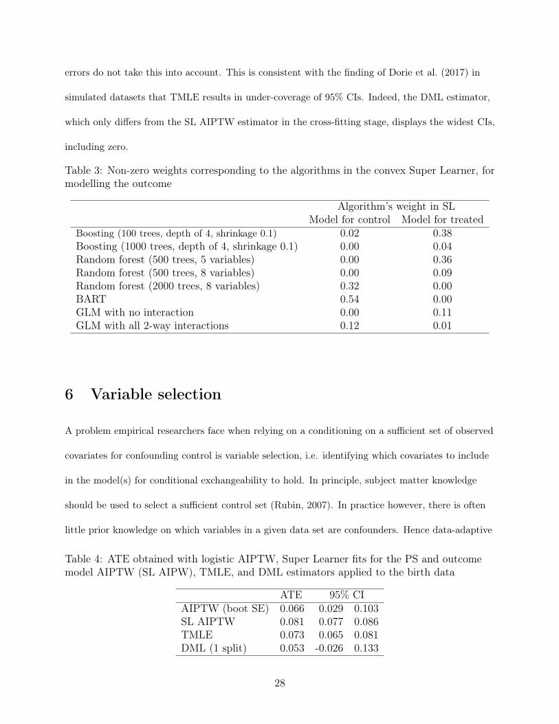
errors do not take this into account. This is consistent with the finding of Dorie et al. (2017) in

simulated datasets that TMLE results in under-coverage of 95% CIs. Indeed, the DML estimator,

which only differs from the SL AIPTW estimator in the cross-fitting stage, displays the widest CIs,

including zero.

Table 3: Non-zero weights corresponding to the algorithms in the convex Super Learner, formodelling the outcome

Algorithm’s weight in SLModel for control Model for treated

Boosting (100 trees, depth of 4, shrinkage 0.1) 0.02 0.38Boosting (1000 trees, depth of 4, shrinkage 0.1) 0.00 0.04Random forest (500 trees, 5 variables) 0.00 0.36Random forest (500 trees, 8 variables) 0.00 0.09Random forest (2000 trees, 8 variables) 0.32 0.00BART 0.54 0.00GLM with no interaction 0.00 0.11GLM with all 2-way interactions 0.12 0.01

6 Variable selection

A problem empirical researchers face when relying on a conditioning on a sufficient set of observed

covariates for confounding control is variable selection, i.e. identifying which covariates to include

in the model(s) for conditional exchangeability to hold. In principle, subject matter knowledge

should be used to select a sufficient control set (Rubin, 2007). In practice however, there is often

little prior knowledge on which variables in a given data set are confounders. Hence data-adaptive

Table 4: ATE obtained with logistic AIPTW, Super Learner fits for the PS and outcomemodel AIPTW (SL AIPW), TMLE, and DML estimators applied to the birth data

ATE 95% CIAIPTW (boot SE) 0.066 0.029 0.103SL AIPTW 0.081 0.077 0.086TMLE 0.073 0.065 0.081DML (1 split) 0.053 -0.026 0.133

28

procedures to select the variables to adjust for become increasingly necessary when the number of

potential confounders is very large. There is a lack of clear guidance about what procedures to use,

and about how to obtain valid inferences after variable selection. In this Section, we consider some

approaches for variable selection when the focus is on the estimation of causal effects.

Decisions on whether to include a covariate in a regression model, whether these are done

manually or by automated methods, such as stepwise regression, are usually based on the strength

of evidence for the residual association with the outcome, by for example, iteratively testing for

significance in models that include or exclude the variable, and comparing the resulting p-value to

a pre-specified significance level. Stepwise models (backwards or forwards selection) are however

widely recognised to perform poorly (Heinze et al., 2018), for two main reasons. First, collinearity

can be an issue, which is especially problematic for forward-selection, while in high-dimensional

settings backward selection may be unfeasible. Second, tests performed during the variable

selection process are not pre-specified, and this is typically not acknowledged in the subsequent

analysis, compromising the validity and the interpretability of subsequent inferences, derived from

models after variable selection.

Decisions about which covariates to adjust for in a regression must ideally be based on the evidence

of confounding, taking into account the covariate-exposure association. Yet causal inference

procedures that only rely on the strength of covariate-treatment relationships (e.g. propensity

score methods) may also be problematic. For example, they may lead to adjusting for variables

that are causes of the exposure only (so-called pure instruments), inducing bias (Vansteelandt

et al., 2012). On the other hand, if variable selection only relies on modelling the outcome, using

for example, lasso regression, it may introduce regularisation bias, due to underestimating

coefficients, and as a result, mistakenly excluding variables with non-zero coefficients.

To address these challenges, Belloni et al. (2014b) proposed a solution that offers principled

29

variable selection, taking into account both the covariate-outcome and the covariate-treatment

assignment association, resulting in valid inferences after variable selection. Their framework,

referred to as “post double selection”, or “double-lasso’, also allows to extend to space of possible

confounding variables to include higher order terms. Following Belloni et al. (2014b), we consider

the partially linear model Yi = g(Xi) + β0Ai + ζi, where Xi a set of confounder-control variables,

and ζi is the error term satisfying E[ζi|Ai,Xi] = 0. We examine the problem of selecting a set of

variables V from among d2 potential variables Wi = f(X), which includes X and transformations

of X as to adequately approximate g(X), and allowing for d2 > N . Crucially, pure instruments, i.e.

variables associated with the treatment but not the outcome, do not need to be identified and

excluded in advance.

We identify covariates for inclusion in our estimators of causal effects in two steps. First we find

those that predict the outcome and in a separate second step those that predict the treatment. A

lasso linear regression calibrated to avoid overfitting is used for both models. In a final step, the

union of the variables selected in either step is used as the confounder control set, to be used in the

causal parameter estimator. The control set can include some additional covariates identified

beforehand.

Belloni et al. (2014b) show that the double lasso results in valid estimates of ATE under the key

assumption of ultra sparsity, i.e. conditional exchangeability holds after controlling for a relatively

small number s <<√N of variables in X not known apriori. Implementation is straightforward,

for example using the glmnet R package. We use cross-validation for choosing the tuning

parameter, following Dukes et al. (2018). Once the confounder control set is selected, a standard

method of estimation is used, for example ordinary least squares estimation of the outcome

regression.

30

6.1 Application of double lasso to the birth data

We now apply the double lasso approach for variable selection to our birth data example. We begin

by running a lasso linear regression (using the glmnet R package) for both outcome and treatment

separately, including all the variables available and using cross-validation to select the penalty.

The union of the variables selected for both models was all 35 available covariates. These variables

are used to control for confounding first in a parametric logistic outcome regression model, which

we use to predict the potential outcomes, and obtain the ATE. We also calculate IPTW and

AIPTW estimates using the weights from a parametric logistic model for the PS. For all estimates

we use bootstrap to obtain SEs.

We then increase the covariate space to include all the two-way interactions between the

covariates, excluding the exposure and the outcome, resulting in a total of 595 covariates. Using

double-lasso on this extended covariate space, we select 156 covariates for the outcome and 89 for

the treatment model, leaving us a union set used for confounding control of 211. We repeat the

three estimators now based on this expanded control set.

Table 5 reports the esimated ATEs and 95 % CIs. The CI’s for the double-lasso outcome

regression were obtained using the non-parametric bootstrap, while the IPTW and AIPTW were

obtained as before using the sandwich SEs. The top panel of the table shows estimates using all

covariates but no interactions, and the bottom panel shows estimates using 72 covariates, including

the main terms and the interactions. The point estimates change very little, implying a minor role

of the interactions in controlling for confounding.

6.2 Collaborative TMLE

Covariate selection for the propensity score can also be done within the TMLE framework.

Previously, we have seen that for a standard TMLE estimator of the ATE, the estimation of the

31

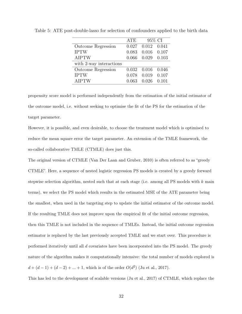
Table 5: ATE post-double-lasso for selection of confounders applied to the birth data

ATE 95% CIOutcome Regression 0.027 0.012 0.041IPTW 0.083 0.016 0.107AIPTW 0.066 0.029 0.103with 2-way interactionsOutcome Regression 0.032 0.016 0.046IPTW 0.078 0.019 0.107AIPTW 0.063 0.026 0.101

propensity score model is performed independently from the estimation of the initial estimator of

the outcome model, i.e. without seeking to optimise the fit of the PS for the estimation of the

target parameter.

However, it is possible, and even desirable, to choose the treatment model which is optimised to

reduce the mean square error the target parameter. An extension of the TMLE framework, the

so-called collaborative TMLE (CTMLE) does just this.

The original version of CTMLE (Van Der Laan and Gruber, 2010) is often referred to as “greedy

CTMLE”. Here, a sequence of nested logistic regression PS models is created by a greedy forward

stepwise selection algorithm, nested such that at each stage (i.e. among all PS models with k main

terms), we select the PS model which results in the estimated MSE of the ATE parameter being

the smallest, when used in the targeting step to update the initial estimator of the outcome model.

If the resulting TMLE does not improve upon the empirical fit of the initial outcome regression,

then this TMLE is not included in the sequence of TMLEs. Instead, the initial outcome regression

estimator is replaced by the last previously accepted TMLE and we start over. This procedure is

performed iteratively until all d covariates have been incorporated into the PS model. The greedy

nature of the algorithm makes it computationally intensive: the total number of models explored is

d+ (d− 1) + (d− 2) + ...+ 1, which is of the order O(d2) (Ju et al., 2017).

This has led to the development of scalable versions (Ju et al., 2017) of CTMLE, which replace the

32

greedy search with a data-adaptive pre-ordering of the candidate PS model estimators. The time

burden of these scalable CTMLE algorithms is of order O(d). Two CTMLE pre-ordering strategies

are proposed: logistic and correlation. The logistic preordering CTMLE constructs an univariable

estimator of the PS for each available covariate, pk with Xk the baseline variable, k = 1, . . . , d.

Using the resulting predicted PS, we construct the clever covariate corresponding to the TMLE for

the ATE, namely h(A, k) = Apk− (1−A)

(1−pk) , and fluctuate the initial estimate of the parameter of

interest µ0 using this clever covariate, (and a logistic log-likelihood) as usual in the TMLE

literature. We obtain the targeted estimate and compute the empirical loss, which could be for

instance the mean sum of squares errors. Finally we order the covariates by increasing value of this

loss.

The correlation pre-ordering is motivated by noting that we would like the k-th covariate added to

the PS model to be that which best explains the current residual, i.e. between Y and current

targeted estimate. Thus, the correlation pre-ordering ranks the covariates based on their

correlation with the residual between Y and the initial outcome regression estimate µ0 (Ju et al.,

2017).

For both pre-orderings, at each step of the CTMLE, we add the variables to the PS prediction

model in this order, as long as the value of the loss function continues to decrease.

Another version of the CTMLE exploits lasso regression for the selection of the variables to be

included in the PS estimation (Ju et al., 2017). This CTMLE algorithm also constructs a sequence

of propensity score estimators, each of them a lasso logistic model with a penalty λk, where k is

monotonically decreasing, and which is “initialised” with λ1 the minimum λ selected by

cross-validation. Then, the corresponding TMLE estimator for the ATE is constructed for each PS

model, finally choosing by cross-validation the TMLE which minimises the loss function (MSE).

The SEs for all CTMLE versions are computed based on the variance of the influence function, as

33

implemented in the R package ctmle.

6.2.1 CTMLE applied to the birth data

We now apply all these variants of CTMLE to the case study. The final logisic pre-ordering

CTMLE is based on a PS model containing nine covariates, including variables indicating the year

of birth, and variables capturing education and socioeconomic status.The CTMLE based on

correlation pre-ordering selected three covariates for the PS, one variable that captures

participation in a social assistance programme, but also two variables that measure the availability

of health care providers in the community. These latter variables are indeed to be expected to have

a strong associaton with the outcome, assisted birth, hence it is not surprising that they were

selected, based on their role in reducing the MSE of the ATE.Finally, the lasso CTMLE is based

on a penalty term 0.000098 chosen by cross-validation, which resulted in all variables having

non-zero coefficients for the PS.

The results are reported on Table 6. The estimated ATEs are somewhat larger than those obtained

using TMLE, all reporting an increase of around 8% in the probability of giving birth assisted by a

health care professional, for those who have social health insurance vs. uninsured. However, the

CTMLE estimate resulting from the lasso, which selected all variables into the PS model, is

(unsurprisingly) very similar to the TMLE estimate reported in Section 5.6, and thus is further

away from the naive estimate than the estimates from CTMLEs that use only a subset of the

variables. Lasso-CTMLE also has wider 95% CIs than the rest, while the greedy CTMLE has the

tightest. This may be an empirical evidence of the bias-variance trade off: due to using less

covariates in the PS, the estimators that use aggressive variable selection for the PS are slightly

biased, but with lower variance.

34

Table 6: ATE obtained with CTML estimators applied to the birth data

ATE 95% CIGreedy CTMLE 0.082 (0.071, 0.094)Scalable CTMLE logistic pre-ordering 0.085 (0.067, 0.104)Scalable CTMLE correlation pre-ordering 0.082 (0.068, 0.097)Lasso CTMLE 0.076 (0.048, 0.105)

7 Further topics

Throughout this chapter, we have seen how machine learning can be used in estimating ATE, by

using it as a prediction tool for outcome regression or PS models. The same logic can be applied to

many other estimation problems where there are nuisance parameters that need to be predicted as

part of the estimation of the parameter of interest.

7.1 Estimating treatment effect heterogeneity

We focused the discussion to the common target parameter, the ATE. Most of the methods

considered are also available for the ATT parameter (see e.g. Chernozhukov et al. (2018)). The

difference between the ATE and ATT stems from heterogeneous treatment effects, and this

heterogeneity – in particular, heterogeneity with respect to observed covariates – in itself can be an

interesting target of causal inference. For example, in the birth cohort example of this paper, we

may be interested in how the effect of health insurance varies by the socioeconomic gradient. To

answer this question, one may either want to specify the “treatment effect function”, a possibly

non-parametric function of the treatment effects as a function of deprivation, and possibly other

covariates such as age. An other approach may be subgroup analysis, based on variables that have

been selected in a data-adaptive way.

Imai et al. (2013) propose a variable selection method using Support Vector Machines, to estimate

heterogeneous treatment effects in randomised trials. Hahn et al. (2017) further develop the BART

35

framework to estimate treatment effect heterogeneity, by flexibly using the estimated propensity

score to correct for regularisation bias. Athey and Imbens (2016) propose a regression tree method,

referred to as “causal trees” to identify subgroups with treatment effect heterogeneity, using

sample-splitting to avoid overfitting. Wager and Athey (2017) extend this idea to random

forest-based algorithms, referred to as “causal forests” for which they establish theoretical

properties. A second interesting question may concern optimal policies: if a health policy maker

has limited resources to provide free insurance for those currently uninsured, what would be an

optimal allocation mechanism that maximimses health benefits? The literature on “optimal policy

learning” is rapidly growing. Kitagawa and Tetenov (2017) focus on estimating optimal policies

from a set of possible policies with limited complexity, while Athey and Wager (2017) further

develop the double-machine learning (Chernozhukov et al., 2018) to estimate optimal policies.

Further approaches have been proposed, for example (Kallus, 2017) based on balancing and within

the TMLE framework (van der Laan and Luedtke, 2015; Luedtke and Chambaz, 2017).

7.2 Instrumental variables

In certain situations, even after adjusting for observed covariates, there may be doubts as to

whether conditional exchageability holds. However, other methods can be used where there is an

instrumental variable (IV) available, that is a variable which is correlated with the exposure but is

not associated with any confounder of the exposure-outcome association, nor is there any pathway

by which the IV affects the outcome, other than through the exposure. Depending on the

additional assumptions the analyst is prepared to make, different estimands can be identified.

Here, we focus on the local average treatment effect (LATE) under monotonic treatment (Angrist

et al., 1996).

Consider the (partially) linear instrumental variable model, which in its simpler form can be

36

thought of as a two-stage procedure, where the first stage consists of a linear regression of the

endogeneous exposure A on the instrument Z, A = α0 + αZ + εa . Then in a second stage, we

regress the outcome on the predicted exposure A, Y = β0 + β1A+ εy.

Usually, the first stage is treated as an estimation step, and the coefficients are obtained using

OLS. In fact, we are only interested in the predicted exposure for each observation, and the

parameters in the first stage are merely nuisance parameters that must be estimated to calculate

the fitted values for exposure. Thus, we can think of this problem directly as a prediction problem,

and use machine learning algorithms for the first stage. This can help alleviate some of the finite

sample bias, often observed in IV estimates, which are typically biased towards the OLS, as a

consequence of overfitting the first stage regression, a problem that is more serious with small

sample sizes or weak instruments (Mullainathan and Spiess, 2017).

A number of recent studies have used ML for the first stage of the IV models. Belloni et al. (2012)

use lasso, while Hansen and Kozbur (2014) use ridge regression. More recently, a TMLE has been

developed for IV models, which uses ML fits also for the initial target parameter estimation (Tóth

and van der Laan, 2016). Double robust IV estimators can also be used with machine learning

predictions for the nuisance models in the second stage, as shown in (Chernozhukov et al., 2018;

DiazOrdaz et al., 2018).

8 Discussion

We have attempted to provide an overview of the current use of ML methods for causal inference,

in the setting of evaluating the average treatment effects of binary static treatments, assuming no

unobserved confounding. We used a case study of an evaluation of a health insurance scheme on

health care utilisation in Indonesia. The case study displayed characteristics typical of applied

37

evaluations: a binary outcome, and a mixture of binary, categorical and continuous covariates. A

practical limitation of the presented case study is the presence of missing data. While for

simplicity, we used a complete case analysis, assuming that missingness does not depend on both

the treatment and the outcome (Bartlett et al., 2015). If this is not the case, the resulting

estimates may be biased. Several options to handle missing data under less restrictive assumptions

exist: e.g. multiple imputation (Rubin, 1987), which is in general valid under missing-at-random

assumptions, or the missing indicator method, which includes indicators for missingness in the set

of potential variables to adjust for, and relies on the assumption that the confounders are only

such when observed (D’Agostino et al., 2001). Another alternative is to use inverse probability of

“being a complete case” weights, which can be easily combined with many of the methods

described in this article (Seaman and White, 2014).

We have highlighted the limitations of naively interpreting the output of machine learning

prediction methods as causal estimates, and provided a review of recent innovations that plug-in

ML prediction of nuisance parameters in ATE estimators. We have demonstrated how ML can

make the estimation of the PS more principled, and also illustrated a multivariate matching

approach that uses ML to data-adaptively select balanced comparison groups. We also highlighted

the limitations of such “design based” approaches: they may not improve balance on variables that

really matter to reduce bias in the estimated ATE, as they cannot easily take into account

information on the relative importance of confounders for the outcome variable.

We gave a brief overview of the possibility of using ML for estimating ATEs via outcome

regressions. We emphasised that obtaining valid confidence intervals after such procedures is

complicated, and the bootstrap is not valid. Some methods, such as BARTs are able to give

inferences based on the corresponding posterior distributions, and have been used in practice with

success (Dorie et al., 2017). Nevertheless, there are currently no theoretical results underpinning

38

its use (Wager and Athey, 2017), and thus BART inferences should be used with caution. Instead,

we illustrated double-robust approaches that combine the strengths of PS estimation and outcome

modelling, and are able to incorporate ML predictors in a principled way. These approaches,

specifically TMLE pioneered by van der Laan and colleagues, and the double machine learning

estimators developed by Chernozokov and colleagues, have appealing theoretical properties and

increasing evidence of their good finite sample performance (Porter et al., 2011; Dorie et al., 2017).

All estimation approaches demonstrated in this article rely on the assumption that selection into

treatment is based on observable covariates only. In many settings of policy evaluations, this

assumption is not tenable. Under such settings, beyond instrumental variable methods (discussed

in Section 7.2), panel data approaches are commonly used to control for one source of unobserved

confounding, that is due to unobservables that remain constant over time. To date, ML approaches

have not been combined with panel data econometric methods. Exceptions are Bajari et al. (2015)

and Chernozhukov et al. (2017) who demonstrate ML approaches for demand estimation using

panel data.

We stress once again that ML methods can improve the estimation of causal effects only once the

identification step has been firmed up and using estimators with appropriate convergence rates, so

that they remain consistent even when using ML fits. However, with the increasing availability of

Big data, in particular in settings with a very large number of covariates, assumptions such as “no

unobserved confounders” may be more plausible (Titiunik, 2015). With such d >> n datasets, ML

methods are indispensable for variable selection as well as the construction of low dimensional

parameters such as average treatment effects. Indeed, many innovations in ML for causal inference

are taking place in such d >> n settings (e.g. Belloni et al. (2011, 2014a); Wager and Athey

(2017)).

Finally, we believe that, paradoxically, ML methods that are often criticized for their ‘’black box”

39

nature, may increase the transparency of applied research. In particular, ensemble learning

algorithms such as the Super Learner, can provide a safeguard against having to hand-pick the

best model or algorithm. ML should be encouraged to enhance expert substantive knowledge when

selecting confounders and model specification.

Acknowledgements

Karla DiazOrdaz was supported by UK Wellcome Trust Institutional Strategic Support Fund–

LSHTM Fellowship 204928/Z/16/Z.

Noémi Kreif gratefully acknowledges her co-authors on the impact evaluation of the Indonesian

public health insurance scheme: Andrew Mirelman, Rodrigo Moreno-Serra, Marc Suhrcke (Centre

for Health Economics, University of York) and Budi Hidayat (University of Indonesia).

Further reading

Athey S. (2017b) Beyond prediction: Using big data for policy problems. Science, 355(6324):

483–485.

Athey, S. and Imbens, G. W., and Wager, S. (2018) Approximate residual balancing: debiased

inference of average treatment effects in high dimensions. Journal of the Royal Statistical

Society: Series B (Statistical Methodology), 80(4):597–623.

Athey, S. and Imbens, G. W. (2017a) The state of applied econometrics: Causality and policy

evaluation. Journal of Economic Perspectives, 31(2):3–32.

Belloni, A., Chernozhukov, V. and Hansen, C. (2014) Inference on Treatment Effects after

40

Selection among High-Dimensional Controls. Review of Economic Studies, 81(August):608–650.

doi10.1093/restud/rdt044.

Chernozhukov, V., Chetverikov, D., Demirer, M., Duflo, E., Hansen, C., and Newey, W. (2017a)

Double/debiased/neyman machine learning of treatment effects. American Economic Review,

107(5):261–65.

Chernozhukov, V., Chetverikov, D., Demirer, M., Duflo, E., Newey, W. and Robins, J. (2018)

Double/debiased machine learning for treatment and structural parameters. The Econometrics

Journal, 21: C1-C68. doi:10.1111/ectj.12097.

Diamond, A. and Sekhon, J. S. (2013) Genetic matching for estimating causal effects: A general

multivariate matching method for achieving balance in observational studies. Review of

Economics and Statistics, 95(3):932–945.

James G., Witten D., Hastie T., and Tibshirani R. (2013) An introduction to statistical learning,

volume 112. Springer.

Kleinberg, J., Ludwig, J., Mullainathan, S., and Obermeyer, Z. (2015) Prediction policy problems.

American Economic Review, 105(5):491–95.

Lee,B. K., Lessler, J. and Stuart,E. A. (2010) Improving propensity score weighting using machine

learning. Statistics in medicine, 29(3):337–346.

McCaffrey, D. F., Ridgeway, G. and Morral, A. R. (2004) Propensity score estimation with boosted

regression for evaluating causal effects in observational studies. Psychological methods, 9(4):403.

Mullainathan, S. and Spiess, J. (2017) Machine learning: an applied econometric approach.

Journal of Economic Perspectives, 31(2):87–106.

41

Polley, E. C. and van der Laan, M. J. (2010) Super learner in prediction. U.C. Berkeley Division of

Biostatistics Working Paper Series Working Paper 266. URL

http://biostats.bepress.com/ucbbiostat/paper266.

van der Laan, M. J. and Gruber, S. (2010) Collaborative double robust targeted maximum

likelihood estimation. International Journal of Biostatistics, 6(1). doi:10.2202/1557-4679.1181.

van der Laan, M. J., and Rose, S. (2011) Targeted learning: causal inference for observational and

experimental data. Springer Science & Business Media.

van der Laan, M. J. and Rubin, D. (2006) Targeted maximum likelihood learning. The

International Journal of Biostatistics, 2(1).

Varian, H. R. (2014) Big data: New tricks for econometrics. Journal of Economic Perspectives, 28

(2):3–28.

References

Abadie, A. and G. W. Imbens (2006). Large sample properties of matching estimators for average

treatment effects. econometrica 74 (1), 235–267.

Abadie, A. and G. W. Imbens (2011). Bias-corrected matching estimators for average treatment

effects. Journal of Business & Economic Statistics 29 (1), 1–11.

Abadie, A. and G. W. Imbens (2016). Matching on the estimated propensity score.

Econometrica 84 (2), 781–807.

Angrist, J. D., G. W. Imbens, and D. B. Rubin (1996). Identification of Causal Effects Using

Instrumental Variables. Journal of the American Statistical Association 91 (434), pp. 444–455.

42

Athey, S. (2017a). Beyond prediction: Using big data for policy problems. Science 355 (6324),

483–485.

Athey, S. (2017b). The impact of machine learning on economics. In Economics of Artificial

Intelligence. University of Chicago Press.

Athey, S. and G. Imbens (2016). Recursive partitioning for heterogeneous causal effects.

Proceedings of the National Academy of Sciences 113 (27), 7353–7360.

Athey, S. and G. W. Imbens (2017). The state of applied econometrics: Causality and policy

evaluation. Journal of Economic Perspectives 31 (2), 3–32.

Athey, S., G. W. Imbens, and S. Wager (2018). Approximate residual balancing: debiased

inference of average treatment effects in high dimensions. Journal of the Royal Statistical

Society: Series B (Statistical Methodology) 80 (4), 597–623.

Athey, S. and S. Wager (2017). Efficient policy learning. arXiv preprint arXiv:1702.02896 .

Austin, P. C. (2009). Some methods of propensity-score matching had superior performance to

others: results of an empirical investigation and monte carlo simulations. Biometrical Journal:

Journal of Mathematical Methods in Biosciences 51 (1), 171–184.

Austin, P. C. (2012). Using ensemble-based methods for directly estimating causal effects: an

investigation of tree-based g-computation. Multivariate behavioral research 47 (1), 115–135.

Bajari, P., D. Nekipelov, S. P. Ryan, and M. Yang (2015). Machine learning methods for demand

estimation. American Economic Review 105 (5), 481–85.

Bang, H. and J. M. Robins (2005). Doubly robust estimation in missing data and causal inference

models. Biometrics 61 (4), 962–973.

43

Bartlett, J. W., O. Harel, and J. R. Carpenter (2015). Asymptotically unbiased estimation of

exposure odds ratios in complete records logistic regression. American journal of

epidemiology 182 (8), 730–736.

Belloni, A., D. Chen, V. Chernozhukov, and C. Hansen (2012). Sparse Models and Methods for

Optimal Instruments With an Application to Eminent Domain. Econometrica 80 (6), 2369–2429.

Belloni, A., V. Chernozhukov, et al. (2011). L1-penalized quantile regression in high-dimensional

sparse models. The Annals of Statistics 39 (1), 82–130.

Belloni, A., V. Chernozhukov, and C. Hansen (2014a). Inference on treatment effects after

selection among high-dimensional controls. The Review of Economic Studies 81 (2), 608–650.

Belloni, A., V. Chernozhukov, and C. Hansen (2014b). Inference on Treatment Effects after

Selection among High-Dimensional Controls †. Review of Economic Studies 81 (August),

608–650.

Bickel, P., F. Götze, and W. van Zwet (1997). Resampling fewer than n observations: Gains,

losses, and remedies for losses. Statistica Sinica 7, 1–31.

Bickel, P. J. and J. Kwon (2001). Inference for semiparametric models: some questions and an

answer. Statistica Sinica 11, 920–936.

Busso, M., J. DiNardo, and J. McCrary (2014). New evidence on the finite sample properties of

propensity score reweighting and matching estimators. Review of Economics and

Statistics 96 (5), 885–897.

Chernozhukov, V., D. Chetverikov, M. Demirer, E. Duflo, C. Hansen, and W. Newey (2017).

Double/debiased/neyman machine learning of treatment effects. American Economic

Review 107 (5), 261–65.

44

Chernozhukov, V., D. Chetverikov, M. Demirer, E. Duflo, C. Hansen, W. Newey, and J. Robins

(2018). Double/debiased machine learning for treatment and structural parameters. The

Econometrics Journal 21 (1), C1–C68.

Chernozhukov, V., M. Goldman, V. Semenova, and M. Taddy (2017). Orthogonal machine

learning for demand estimation: High dimensional causal inference in dynamic panels. arXiv

preprint arXiv:1712.09988 .

Cole, S. R. and C. E. Frangakis (2009). The consistency statement in causal inference: a definition

or an assumption? Epidemiology 20 (1), 3–5.

D’Agostino, R., W. Lang, M. Walkup, T. Morgan, and A. Karter (2001, Dec). Examining the

impact of missing data on propensity score estimation in determining the effectiveness of

self-monitoring of blood glucose (smbg). Health Services and Outcomes Research

Methodology 2 (3), 291–315.

Diamond, A. and J. S. Sekhon (2013). Genetic matching for estimating causal effects: A general

multivariate matching method for achieving balance in observational studies. Review of

Economics and Statistics 95 (3), 932–945.

DiazOrdaz, K., R. Daniel, and N. Kreif (2018, February). Data-adaptive doubly robust

instrumental variable methods for treatment effect heterogeneity. ArXiv e-prints.

Dorie, V., J. Hill, U. Shalit, M. Scott, and D. Cervone (2017). Automated versus do-it-yourself

methods for causal inference: Lessons learned from a data analysis competition. arXiv preprint

arXiv:1707.02641 .

Dukes, O., V. Avagyan, and S. Vansteelandt (2018). High-dimensional doubly robust tests for

regression parameters. arXiv preprint arXiv:1805.06714 .

45

Eliseeva, E., A. E. Hubbard, and I. B. Tager (2013). An application of machine learning methods

to the derivation of exposure-response curves for respiratory outcomes.

Farrell, M. H. (2015). Robust inference on average treatment effects with possibly more covariates

than observations. Journal of Econometrics 189 (1), 1–23.

Friedman, J., T. Hastie, and R. Tibshirani (2001). The elements of statistical learning, Volume 1.

Springer series in statistics New York, NY, USA:.

Gruber, S., R. W. Logan, I. Jarrín, S. Monge, and M. A. Hernán (2015). Ensemble learning of

inverse probability weights for marginal structural modeling in large observational datasets.

Statistics in medicine 34 (1), 106–117.

Gruber, S. and M. J. Van Der Laan (2009). Targeted maximum likelihood estimation: A gentle

introduction.

Gruber, S. and M. J. van der Laan (2010). A targeted maximum likelihood estimator of a causal

effect on a bounded continuous outcome. The International Journal of Biostatistics 6 (1).

Gruber, S. and M. J. van der Laan (2011). tmle: An r package for targeted maximum likelihood

estimation.

Hahn, P. R., J. S. Murray, and C. M. Carvalho (2017). Bayesian regression tree models for causal

inference: regularization, confounding, and heterogeneous effects.

Hainmueller, J. (2012). Entropy balancing for causal effects: A multivariate reweighting method to

produce balanced samples in observational studies. Political Analysis 20 (1), 25–46.

Hansen, C. and D. Kozbur (2014). Instrumental variables estimation with many weak instruments

using regularized jive. Journal of Econometrics 182 (2), 290–308.

46

Heinze, G., C. Wallisch, and D. Dunkler (2018). Variable selection – A review and

recommendations for the practicing statistician.

Hill, J. L. (2011). Bayesian nonparametric modeling for causal inference. Journal of Computational

and Graphical Statistics 20 (1), 217–240.

Hirano, K., G. W. Imbens, and G. Ridder (2003). Efficient estimation of average treatment effects

using the estimated propensity score. Econometrica 71 (4), 1161–1189.

Imai, K. and M. Ratkovic (2014). Covariate balancing propensity score. Journal of the Royal

Statistical Society: Series B (Statistical Methodology) 76 (1), 243–263.

Imai, K., M. Ratkovic, et al. (2013). Estimating treatment effect heterogeneity in randomized

program evaluation. The Annals of Applied Statistics 7 (1), 443–470.

Imbens, G. W. and J. M. Wooldridge (2009). Recent developments in the econometrics of program

evaluation. Journal of economic literature 47 (1), 5–86.

James, G., D. Witten, T. Hastie, and R. Tibshirani (2013). An introduction to statistical learning,

Volume 112. Springer.

Ju, C., S. Gruber, S. D. Lendle, A. Chambaz, J. M. Franklin, R. Wyss, S. Schneeweiss, and M. J.

van der Laan (2017). Scalable collaborative targeted learning for high-dimensional data.

Statistical methods in medical research, 0962280217729845.

Ju, C., R. Wyss, J. M. Franklin, S. Schneeweiss, J. Häggström, and M. J. van der Laan (2017).

Collaborative-controlled LASSO for constructing propensity score-based estimators in

high-dimensional data. Statistical Methods in Medical Research.

Kallus, N. (2017). Balanced policy evaluation and learning. arXiv preprint arXiv:1705.07384 .

47

Kang, J. D., J. L. Schafer, et al. (2007). Demystifying double robustness: A comparison of

alternative strategies for estimating a population mean from incomplete data. Statistical

science 22 (4), 523–539.

Kapelner, A. and J. Bleich (2013). bartmachine: Machine learning with bayesian additive

regression trees. arXiv preprint arXiv:1312.2171 .

Kennedy, E. H. (2016). Semiparametric Theory and Empirical Processes in Causal Inference,

Chapter Statistical Causal Inferences and Their Applications in Public Health Research, pp.

141–167. Cham: Springer International Publishing.

Kitagawa, T. and A. Tetenov (2017). Who should be treated? empirical welfare maximization

methods for treatment choice.

Kleinberg, J., J. Ludwig, S. Mullainathan, and Z. Obermeyer (2015). Prediction policy problems.

American Economic Review 105 (5), 491–95.

Kreif, N., R. Grieve, R. Radice, and J. S. Sekhon (2013). Regression-adjusted matching and

double-robust methods for estimating average treatment effects in health economic evaluation.

Health Services and Outcomes Research Methodology 13 (2-4), 174–202.

Kreif, N., S. Gruber, R. Radice, R. Grieve, and J. S. Sekhon (2016). Evaluating treatment

effectiveness under model misspecification: a comparison of targeted maximum likelihood

estimation with bias-corrected matching. Statistical methods in medical research 25 (5),

2315–2336.

Kreif, N., A. Mirelman, R. Moreno Serra, B. Hidayat, D. Erlannga, and M. Suhrcke (2018).

Evaluating the impact of public health insurance reforms on infant mortality in Indonesia.

Technical report.

48

Lee, B. K., J. Lessler, and E. A. Stuart (2010). Improving propensity score weighting using

machine learning. Statistics in medicine 29 (3), 337–346.

Leeb, H. and M. P. Benedikt (2008). Can One Estimate The Unconditional Distribution of

Post-Model-Selection Estimators? Econometric Theory 24, 338–376.

Luedtke, A. and A. Chambaz (2017). Faster rates for policy learning. arXiv preprint

arXiv:1704.06431 .

Lunceford, J. K. and M. Davidian (2004). Stratification and weighting via the propensity score in

estimation of causal treatment effects: a comparative study. Statistics in medicine 23 (19),

2937–2960.

McCaffrey, D. F., G. Ridgeway, and A. R. Morral (2004). Propensity score estimation with boosted

regression for evaluating causal effects in observational studies. Psychological methods 9 (4), 403.

Mebane Jr, W. R., J. S. Sekhon, et al. (2011). Genetic optimization using derivatives: the rgenoud

package for r. Journal of Statistical Software 42 (11), 1–26.

Mullainathan, S. and J. Spiess (2017). Machine learning: an applied econometric approach.

Journal of Economic Perspectives 31 (2), 87–106.

Pearl, J. (2010). On the consistency rule in causal inference: axiom, definition, assumption, or

theorem? Epidemiology 21 (6), 872–875.

Petersen, M. L. (2014). Applying a causal road map in settings with time-dependent confounding.

Epidemiology (Cambridge, Mass.) 25 (6), 898.

Petersen, M. L., K. E. Porter, S. Gruber, Y. Wang, and M. J. van der Laan (2012). Diagnosing

49

and responding to violations in the positivity assumption. Statistical methods in medical

research 21 (1), 31–54.

Pirracchio, R. and M. Carone (2018). The Balance Super Learner: A robust adaptation of the

Super Learner to improve estimation of the average treatment effect in the treated based on

propensity score matching. Statistical Methods in Medical Research 27 (8), 2504–2518.

Pirracchio, R., M. L. Petersen, and M. van der Laan (2015). Improving propensity score

estimators’ robustness to model misspecification using super learner. American journal of

epidemiology 181 (2), 108–119.

Pirracchio, R., M. Resche-Rigon, and S. Chevret (2012). Evaluation of the propensity score

methods for estimating marginal odds ratios in case of small sample size. BMC medical research

methodology 12 (1), 70.

Polley, E. C. and M. J. van der Laan (2010, May). Super learner in prediction. U.C. Berkeley

Division of Biostatistics Working Paper Series Working Paper 266.

Porter, K. E., S. Gruber, M. J. van der Laan, and J. S. Sekhon (2011). The relative performance of

targeted maximum likelihood estimators. The international journal of biostatistics 7 (1), 1–34.

Robins, J., M. Sued, Q. Lei-Gomez, and A. Rotnitzky (2007). Comment: Performance of

double-robust estimators when" inverse probability" weights are highly variable. Statistical

Science 22 (4), 544–559.

Robins, J. M., M. A. Hernan, and B. Brumback (2000). Marginal structural models and causal

inference in epidemiology. Epidemiology 11 (5), 550–560.

Robins, J. M., A. Rotnitzky, and L. P. Zhao (1994). Estimation of regression coefficients when

50

some regressors are not always observed. Journal of the American statistical

Association 89 (427), 846–866.

Robins, J. M., A. Rotnitzky, and L. P. Zhao (1995). Analysis of semiparametric regression models

for repeated outcomes in the presence of missing data. Journal of the american statistical

association 90 (429), 106–121.

Robinson, P. M. (1988). Root-n-consistent semiparametric regression. Econometrica: Journal of

the Econometric Society , 931–954.

Rose, S. (2013). Mortality risk score prediction in an elderly population using machine learning.

American journal of epidemiology 177 (5), 443–452.

Rosenbaum, P. R. and D. B. Rubin (1983). The central role of the propensity score in

observational studies for causal effects. Biometrika 70 (1), 41–55.

Rosenbaum, P. R. and D. B. Rubin (1984). Reducing bias in observational studies using

subclassification on the propensity score. Journal of the American statistical

Association 79 (387), 516–524.

Rubin, D. B. (1978). Bayesian inference for causal effects: The role of randomization. The Annals

of statistics, 34–58.

Rubin, D. B. (1987). In discussion of Tanner, M.\ A.\ and Wong, W.\ H.\, The calculation of

posterior distributions by data augmentation. Journal of the American Statistical

Association 82, 543–546.

Rubin, D. B. (2005). Causal inference using potential outcomes: Design, modeling, decisions.

Journal of the American Statistical Association 100 (469), 322–331.

51

Rubin, D. B. (2007). The design versus the analysis of observational studies for causal effects:

parallels with the design of randomized trials. Statistics in medicine 26 (1), 20–36.

Rubin, D. B. and N. Thomas (1996). Matching using estimated propensity scores: relating theory

to practice. Biometrics, 249–264.

Rubin, D. B. and N. Thomas (2000). Combining propensity score matching with additional

adjustments for prognostic covariates. Journal of the American Statistical Association 95 (450),

573–585.

Seaman, S. and I. White (2014). Inverse probability weighting with missing predictors of treatment

assignment or missingness. Communications in Statistics - Theory and Methods 43 (16),

3499–3515.

Seaman, S. R. and S. Vansteelandt (2018). Introduction to Double Robust Methods for Incomplete

Data. Statistical Science 33 (2), 184–197.

Sekhon, J. S. (2011). Multivariate and propensity score matching software with automated balance

optimization: the matching package for r.

Setoguchi, S., S. Schneeweiss, M. A. Brookhart, R. J. Glynn, and E. F. Cook (2008). Evaluating

uses of data mining techniques in propensity score estimation: a simulation study.

Pharmacoepidemiology and drug safety 17 (6), 546–555.

Stuart, E. A. (2010). Matching methods for causal inference: A review and a look forward.

Statistical science: a review journal of the Institute of Mathematical Statistics 25 (1), 1.

Titiunik, R. (2015). Can big data solve the fundamental problem of causal inference? PS: Political

Science & Politics 48 (1), 75–79.

52

Tóth, B. and M. J. van der Laan (2016). {TMLE} for Marginal Structural Models Based on an

Instrument. U.C. Berkeley Division of Biostatistics Working Paper Series. Working Paper 350..

van der Laan, M. J. and S. Dudoit (2003, November). Unified cross-validation methodology for

selection among estimators and a general cross-validated adaptive epsilon-net estimator: Finite

sample oracle inequalities and examples. U.C. Berkeley Division of Biostatistics Working Paper

Series Working Paper 130.

Van Der Laan, M. J. and S. Gruber (2010). Collaborative double robust targeted maximum

likelihood estimation. International Journal of Biostatistics 6 (1).

van der Laan, M. J. and A. R. Luedtke (2014). Targeted learning of an optimal dynamic

treatment, and statistical inference for its mean outcome.

van der Laan, M. J. and A. R. Luedtke (2015). Targeted learning of the mean outcome under an

optimal dynamic treatment rule. Journal of causal inference 3 (1), 61–95.

van der Laan, M. J., E. C. Polley, and A. E. Hubbard (2007, July). Super learner. U.C. Berkeley

Division of Biostatistics Working Paper Series Working Paper 222.

van der Laan, M. J. and J. M. Robins (2003). Unified methods for censored longitudinal data and

causality. Springer Science & Business Media.

Van der Laan, M. J. and S. Rose (2011). Targeted learning: causal inference for observational and

experimental data. Springer Science & Business Media.

Van Der Laan, M. J. and D. Rubin (2006). Targeted maximum likelihood learning. The

International Journal of Biostatistics 2 (1).

53

van der Vaart, A. (2014). Higher Order Tangent Spaces and Influence Functions. Statistical

Science 29 (4), 679–686.

VanderWeele, T. J. (2009). Concerning the consistency assumption in causal inference.

Epidemiology 20 (6), 880–883.

Vansteelandt, S., M. Bekaert, and G. Claeskens (2012). On model selection and model

misspecification in causal inference. Statistical Methods in Medical Research 21 (1), 7–30.

Varian, H. R. (2014). Big data: New tricks for econometrics. Journal of Economic

Perspectives 28 (2), 3–28.

Wager, S. and S. Athey (2017). Estimation and inference of heterogeneous treatment effects using

random forests. Journal of the American Statistical Association (just-accepted).

Westreich, D., S. R. Cole, M. J. Funk, M. A. Brookhart, and T. Stürmer (2011). The role of the

c-statistic in variable selection for propensity score models. Pharmacoepidemiology and drug

safety 20 (3), 317–320.

Westreich, D., J. Lessler, and M. J. Funk (2010). Propensity score estimation: neural networks,

support vector machines, decision trees (cart), and meta-classifiers as alternatives to logistic

regression. Journal of clinical epidemiology 63 (8), 826–833.

Wyss, R., A. R. Ellis, M. A. Brookhart, C. J. Girman, M. Jonsson Funk, R. LoCasale, and

T. Stürmer (2014). The role of prediction modeling in propensity score estimation: an

evaluation of logistic regression, bcart, and the covariate-balancing propensity score. American

journal of epidemiology 180 (6), 645–655.

Zhang, P. (1993). Model selection via multifold cross validation. The Annals of Statistics, 299–313.

54

Zhu, Y., D. L. Coffman, and D. Ghosh (2015). A boosting algorithm for estimating generalized

propensity scores with continuous treatments. Journal of causal inference 3 (1), 25–40.

Zubizarreta, J. R. (2012). Using mixed integer programming for matching in an observational

study of kidney failure after surgery. Journal of the American Statistical Association 107 (500),

1360–1371.

55