Embed Size (px)
Citation preview

Machine Learning Based Delay Tolerant
Protocols for Underwater Acoustic
Wireless Sensor Networks
Lin Zou
School of Electrical, Electronic and Computer Engineering
The University of Western Australia
This thesis is presented for the degree of
Doctor of Philosophy
September 2014


Declaration
This is to certify that:
• the thesis contains no material that has been accepted for the
award of any other degree or diploma in any university or other
tertiary institution and, to the best of my knowledge and belief,
contains no material previously published written by another
person, except where due reference has been made in the text,
• the thesis comprises only my original work towards the PhD,
• due acknowledgement has been made in the text to all other
material used,
• the thesis is less than 100,000 words in length, exclusive of tables,
maps, bibliographies and appendices,
• I give consent to this copy of the thesis, when deposited in the
University Library, being available for loan, photocopying and
dissemination through the library digital thesis collection.
Lin Zou, September 2014
i

ii

Acknowledgements
First and foremost, I would like to sincerely express my gratitude to
my supervisors, Dr. David (Defeng) Huang and Dr. Roberto Togneri,
for their support during the course of my studies. Without their
enthusiasm, dedication, and confidence in me, this work would have
been impossible. For the past few years, they has put great effort into
helping me find direction and have assisted me in conducting this
research. I have often benefited from their knowledge and experience
in both my research and life. Thanks Dr. Huang and Dr. Togneri for
offering me such a rewarding experience during the course of my PhD
studies.
Also, many thanks to my colleagues in the research group SPWCL at
the University of Western Australia for their insightful discussions and
social activities. I would especially like to express my appreciation to
Prof. Angela (Yingjun) Zhang and her group members at the Chinese
University of Hong Kong (CUHK). It was a great pleasure to have an
opportunity to work with them at CUHK as a visiting scholar. Their
insights, discussions and generous help have led me to my fruitful
research. I would also like to thank my parents and my husband for
their understanding, support and most of all, their love over the past
years.
Finally, I also gratefully acknowledge my host institution, the School
of Electrical, Electronic and Computer Engineering at the University
of Western Australia, and the Endeavor Scholarship Office for their
financial and administrative support during my term.
iii

iv

Publications
BOOK CHAPTER
• L. Jin, D. Huang, Y.J. Zhang and L. Zou, “Cognitive acous-
tics: a way to extend the lifetime of underwater acoustic sensor
networks,” in Cognitive Communications: Distributed Artificial
Intelligence (DAI), Regulatory Policy & Economics. John Wiley
& Sons, 2012.
CONFERENCE
• L. Zou, D. Huang, R. Togneri, “A Neural-Q-Learning Based Ap-
proach for Delay Tolerant Underwater Acoustic Wireless Sensor
Networks”, Proceedings of CCSCI2014, January 2014, Toronto,
Canada, accepted October 2013.
• L. Zou, D. Huang, R. Togneri, “A Q-Learning Based Approach
for Delay Tolerant Underwater Acoustic Wireless Sensor Net-
works”, Proceedings of APWCS2013, August 2013, Seoul, Ko-
rea, accepted June 2013.
v

vi

I would like to dedicate this thesis to my loving parents ...
vii

viii
Abstract
In recent years, the developments of underwater acoustic wireless sen-
sor networks (UA-WSNs) have attracted considerable research inter-
est due to their capabilities to support underwater missions. Under-
water acoustic communication channels are featured with large at-
tenuation, long propagation delay and constrained bandwidth, which
limit communications between sensors and make the system intermit-
tent. As a result, delay tolerance is one of the major design concerns
for supporting UA-WSNs to carry out tasks in harsh subsea envi-
ronments. Although a number of delay tolerant schemes have been
proposed for terrestrial wireless sensor networks, the fundamental dif-
ferences between underwater acoustic channels and radio frequency
channels make those schemes perform poorly in subsea environments.
Therefore, it is desirable to develop a feasible, reliable and robust pro-
tocol for high-speed underwater acoustic wireless communications. In
this dissertation, we present a family of delay tolerant protocols for
UA-WSNs, which employ reinforcement learning algorithms.
In the proposed system, a UA-WSN consisting of a number of static
sensors and a mobile ferry is modeled as a single agent reinforcement
learning system. The sensors are assumed to be sparsely-distributed,
energy-constrained, stationary, and consequently are not capable of
peer to peer sensor communications. For the purpose of conserving
energy, each sensor periodically transits between the active state and
the sleep state. A ferry is employed to travel around the deployment
field to collect, carry and deliver data packets between sensors. A
specific position where the ferry contacts with a specific sensor is
known as a way-point which is fixed at the position of its host sensor.
The ferry acts as the intelligent agent of the employed reinforcement
ix

learning algorithm, which has the freedom to determine the order of
the way-points to be visited according to its independent learning. By
using the proposed protocol, the ferry is capable of learning from the
environment and then adaptively adjusting the relevant parameters of
the networks. Extensive simulation results demonstrate the feasibility
of the proposed protocol which achieves a remarkable improvement of
system performance in comparison with existing protocols.
For the purpose of improving the performance and flexility of the pro-
posed system, we enable the dynamic position of way-points within
the transmission range of their host sensors. An artificial neural net-
work algorithm based Neural-Q-Learning (NQL) protocol is proposed
to enable the ferry (i.e. the NQL agent) to find an efficient and rel-
atively short traveling route which inter-connects the optimized way-
points to deliver data packets between sensors. Compared with the
conventional Q-Learning algorithms, the system agent avoids search-
ing a large or infinite lookup table by searching the optimal action
from a continuous q-curve produced by the Neural-Q-Learning algo-
rithm. Simulation results show that the NQL system improves the
performance by enabling the ferry to determine the optimal position
of way-points in a two-dimensional continuous space, which comprise
an efficient traveling route to reduce the delivery delay and delivery
cost while maximizing the meeting probabilities between the ferry and
sensors.
Finally, the system is extended to a cooperative multi-agent reinforce-
ment learning (MARL) based NQL protocol (named MNQL protocol).
The proposed MNQL system employs the joint action learner algo-
rithm (JAL) to coordinate the actions of multiple ferries, each of which
is modeled as an individual and independent intelligent agent of the
system and treats the actions of other ferries as part of the environ-
ment. Since the global information (e.g. states and actions of other
ferries) is not fully observable for each individual ferry, each ferry em-
ploys a local database to store the most recent action and state of
other ferries which are used by a behavior predictor to estimate the
x

possible action and state of other ferries when direct communications
are infeasible. Compared with the single agent based approaches,
the MNQL system benefits from the cooperative actions among the
ferries.
We analyzed the performance of the proposed protocols in underwater
acoustic wireless sensor networks with various topologies. Compared
with the existing delay tolerant protocols, the proposed reinforcement
learning algorithm based protocols reduce the delivery delay and de-
livery cost by enabling the ferry to find an efficient and relatively short
traveling route which inter-connects the optimized way-points to de-
liver data packets between sensors. The employments of the artificial
neural network algorithm and the multi-agent reinforcement learning
algorithm improve the system performance further.
xi

xii

Contents
Contents xiii
List of Figures xvii
List of Tables xix
List of Acronyms xxi
1 Introduction 1
1.1 Background . . . . . . . . . . . . . . . . . . . . . . . . . . . . . . 1
1.2 Dissertation Contributions . . . . . . . . . . . . . . . . . . . . . . 3
1.3 Dissertation Organization . . . . . . . . . . . . . . . . . . . . . . 5
2 A Reinforcement Learning Based Energy Efficient Protocol for
UA-WSNs and its Implementation 7
2.1 Introduction . . . . . . . . . . . . . . . . . . . . . . . . . . . . . . 7
2.2 Related Works . . . . . . . . . . . . . . . . . . . . . . . . . . . . . 9
2.2.1 Underwater Acoustic Communications . . . . . . . . . . . 9
2.2.2 Q-Learning Algorithm . . . . . . . . . . . . . . . . . . . . 12
2.3 System Descriptions . . . . . . . . . . . . . . . . . . . . . . . . . 15
2.3.1 System State Space . . . . . . . . . . . . . . . . . . . . . . 18
2.3.2 Action Set . . . . . . . . . . . . . . . . . . . . . . . . . . . 18
2.3.3 Reward Function . . . . . . . . . . . . . . . . . . . . . . . 18
2.4 Simulations . . . . . . . . . . . . . . . . . . . . . . . . . . . . . . 22
2.4.1 Configurations . . . . . . . . . . . . . . . . . . . . . . . . . 22
2.4.2 Simulation Results . . . . . . . . . . . . . . . . . . . . . . 22
xiii

CONTENTS
2.5 Conclusion . . . . . . . . . . . . . . . . . . . . . . . . . . . . . . . 25
3 A Neural-Q-Learning Based Approach for Delay Tolerant Un-
derwater Wireless Sensor Networks 27
3.1 Introduction . . . . . . . . . . . . . . . . . . . . . . . . . . . . . . 27
3.2 Related Work . . . . . . . . . . . . . . . . . . . . . . . . . . . . . 30
3.2.1 The Artificial Neural Network . . . . . . . . . . . . . . . . 30
3.2.2 The Neural-Q-Learning Algorithm . . . . . . . . . . . . . . 31
3.3 System Description . . . . . . . . . . . . . . . . . . . . . . . . . . 33
3.3.1 Neural-Q-Learning Framework . . . . . . . . . . . . . . . . 35
3.3.1.1 System State Space . . . . . . . . . . . . . . . . . 35
3.3.1.2 Optimal Action and Action Set . . . . . . . . . . 36
3.3.2 Generating the Q-Curve . . . . . . . . . . . . . . . . . . . 37
3.3.2.1 The ANN Implementation . . . . . . . . . . . . . 38
3.3.2.2 The Wire-Fitting Function . . . . . . . . . . . . . 40
3.3.3 Improvement of the ANN and the Q-Curve . . . . . . . . . 40
3.3.3.1 Evaluation of the Practical Quality Value . . . . 40
3.3.3.2 Repositioning Wires with Gradient-Descent Method 43
3.3.3.3 Training ANN with Back Propagation . . . . . . 44
3.4 Simulation . . . . . . . . . . . . . . . . . . . . . . . . . . . . . . . 44
3.4.1 Configurations . . . . . . . . . . . . . . . . . . . . . . . . . 45
3.4.2 Simulation Results . . . . . . . . . . . . . . . . . . . . . . 45
3.4.2.1 Performance of the Neural-Q-Learning Based Pro-
tocol . . . . . . . . . . . . . . . . . . . . . . . . . 45
3.4.2.2 Performance Comparison with Existing Protocols 46
3.5 Conclusion . . . . . . . . . . . . . . . . . . . . . . . . . . . . . . . 50
4 Multiple Ferries Neural-Q-Learning Based Approach for Delay
Tolerant Underwater Acoustic Wireless Sensor Networks 53
4.1 Introduction . . . . . . . . . . . . . . . . . . . . . . . . . . . . . . 53
4.2 Related Work . . . . . . . . . . . . . . . . . . . . . . . . . . . . . 55
4.3 System Description . . . . . . . . . . . . . . . . . . . . . . . . . . 57
4.3.1 The Cooperative Multi-agent Neural-Q-Learning Framework 58
4.3.1.1 System State Space . . . . . . . . . . . . . . . . . 58
xiv

CONTENTS
4.3.1.2 Optimal Action and Action Set . . . . . . . . . . 59
4.3.2 Generating the Q-Curve . . . . . . . . . . . . . . . . . . . 61
4.3.3 Improvement of the ANN and the Q-Curve . . . . . . . . . 62
4.3.3.1 Evaluation of the Practical Quality Value . . . . 62
4.3.3.2 Agent Behavior Prediction . . . . . . . . . . . . . 63
4.4 Simulation . . . . . . . . . . . . . . . . . . . . . . . . . . . . . . . 65
4.4.1 Configurations . . . . . . . . . . . . . . . . . . . . . . . . . 65
4.4.2 Simulation Results . . . . . . . . . . . . . . . . . . . . . . 66
4.4.2.1 Performance of the MNQL Protocol . . . . . . . 66
4.4.2.2 Performance Comparison with Existing Protocols 69
4.5 Conclusion . . . . . . . . . . . . . . . . . . . . . . . . . . . . . . . 75
5 Conclusions and Future Work 77
5.1 Conclusions . . . . . . . . . . . . . . . . . . . . . . . . . . . . . . 77
5.2 Future Work . . . . . . . . . . . . . . . . . . . . . . . . . . . . . . 79
References 81
xv

CONTENTS
xvi
List of Figures
2.1 The lower and upper boundaries of an underwater acoustic com-
munication channel and the corresponding energy loss versus the
propagation distance [59] . . . . . . . . . . . . . . . . . . . . . . . 12
2.2 System state and action set . . . . . . . . . . . . . . . . . . . . . 19
2.3 delivery delay versus speed of ferry node . . . . . . . . . . . . . . 24
2.4 Ferry node’s traveling distance per delivered packet versus speed
of ferry node . . . . . . . . . . . . . . . . . . . . . . . . . . . . . . 24
2.5 Average meeting probabilities versus speed of ferry node . . . . . 26
2.6 Variance of meeting probability versus speed of ferry node . . . . 26
3.1 A three-layer artificial neural network . . . . . . . . . . . . . . . . 32
3.2 Flow chart of the neural Q-learning algorithm . . . . . . . . . . . 34
3.3 System state and action set . . . . . . . . . . . . . . . . . . . . . 37
3.4 The polar coordinates of a way-point relative to its host sensor . . 38
3.5 The structure of ANN employed in the proposed system . . . . . 39
3.6 NQL: the average delivery delay versus ferry speed . . . . . . . . 47
3.7 NQL: the ferry’s traveling distance per delivered packet versus ferry
speed . . . . . . . . . . . . . . . . . . . . . . . . . . . . . . . . . . 47
3.8 NQL: the average delivery delay versus pm,max . . . . . . . . . . . 48
3.9 NQL: the ferry’s traveling distance per delivered packet versus pm,max 48
3.10 Delivery delay versus ferry speed . . . . . . . . . . . . . . . . . . 51
3.11 Ferry’s traveling distance per delivered packet versus ferry speed . 51
3.12 Delivery delay versus pm,max . . . . . . . . . . . . . . . . . . . . . 52
3.13 Ferry’s traveling distance per delivered packet versus pm,max . . . 52
xvii

LIST OF FIGURES
4.1 Flow chart of the cooperative MNQL algorithm . . . . . . . . . . 59
4.2 System state and action set . . . . . . . . . . . . . . . . . . . . . 61
4.3 total delivered packets versus pm,max . . . . . . . . . . . . . . . . 67
4.4 delivery delay versus pm,max . . . . . . . . . . . . . . . . . . . . . 67
4.5 Ferry’s traveling distance per delivered packet versus pm,max . . . 68
4.6 total delivered packets versus speed . . . . . . . . . . . . . . . . . 68
4.7 delivery delay versus speed . . . . . . . . . . . . . . . . . . . . . . 70
4.8 Ferry’s traveling distance per delivered packet versus speed . . . . 70
4.9 total delivered packets versus pm,max . . . . . . . . . . . . . . . . 72
4.10 delivery delay versus pm,max . . . . . . . . . . . . . . . . . . . . . 72
4.11 Ferry’s traveling distance per delivered packet versus pm,max . . . 74
4.12 total delivered packets versus speed . . . . . . . . . . . . . . . . . 74
4.13 delivery delay versus speed . . . . . . . . . . . . . . . . . . . . . . 76
4.14 Ferry’s traveling distance per delivered packet versus speed . . . . 76
xviii

List of Tables
2.1 The feasible bandwidth Btx(d), lower boundary fl(d) and upper
boundary fu(d) corresponding to propagation distance d . . . . . 13
xix

LIST OF TABLES
xx

List of Acronyms
ANN Artificial Neural Network
AODV Ad hoc On-demand Distance Vector protocol
AUV Autonomous Underwater Vehicle
DM Data Mule
DVF Distributed Value Function
IL Independent Learner
JAL Joint Action Learner
MANET Mobile Ad-hoc wireless Network
MARL Multi-Agent Reinforcement Learning
MDP Markov Decision Process
MF Message Ferry
MNQL Multi-Agent Neural-Q-Learning
NQL Neural-Q-Learning
OFDM Orthogonal Frequency-Division Multiplexing
PSD power spectral density
QL Q-Learning
xxi

LIST OF ACRONYMS
RL Reinforcement Learning
RW Random Walk
SARL Single-Agent Reinforcement Learning
SNR Signal to Noise Ratio
SP Shortest Path
UA-WSNs Underwater Acoustic Wireless Sensor Networks
xxii

Chapter 1
Introduction
1.1 Background
Over 70 percent of the Earth’s surface is covered by the ocean, but more than
95 percent of which remains unexplored [23, 76]. For exploring and exploiting
the unknown subsea world, it is desirable to develop effective and efficient com-
munication means to support underwater missions such as oceanographic data
collection, environment monitoring, and offshore oil and gas exploration.
Most underwater wireless communications use acoustic waves since electro-
magnetic waveforms, such as radio and light, hardly propagate to a distance long
enough for most practical applications due to the severe attenuation of seawater
[49]. Researches in recent decades have revealed that the underwater acoustic
communication channels are featured with large attenuation, long propagation
delay, high bit error rate and limited feasible bandwidth [2, 40]. Moreover,
many recent underwater acoustic communication researches focus on the fully
distributed underwater acoustic wireless sensor networks (UA-WSNs) since the
centralized approach is not robust especially when communication is limited and
failures are highly probable [65, 66, 71, 80]. Due to the significant attenuation
and noise interference in underwater acoustic communication channels, the re-
quired transmission power may be many times greater than that in terrestrial
communication systems [60]. For the purpose of energy conservation, the trans-
mission range of acoustic sensors in UA-WSNs is usually much shorter than that
of the terrestrial counterparts, which limits communications between sensors. As
1
1. INTRODUCTION
a result, in UA-WSNs which are usually envisaged to monitor much larger areas
than those on the ground, the energy-constrained sensors are sparsely-distributed
in a relatively large field and are not capable of providing reliable peer to peer
sensor communications. In some cases, even an end-to-end connection between
a source and a destination may never be present due to the intermittent con-
nections among sensors. In such communication environments, some existing ad
hoc routing protocols such as the Ad hoc On-Demand Distance Vector (AODV)
routing protocol [67] and the Dynamic Source Routing (DSR) protocol [45] fail
to establish routes. Moreover, the slow propagation speed of acoustic signals in
underwater environments and the very limited bandwidth cause remarkable prop-
agation delays which significantly challenge the networking concepts developed
for their terrestrial counterparts where propagation delay is usually negligible.
Therefore, it is essential to develop an effective and efficient delay tolerant scheme
for high-speed UA-WSN systems.
The Delay Tolerant Network (DTN) is one of the recent approaches to such
intermittent network architectures [12, 43], which have the potential to support
a wide range of applications in underwater environments. The development of
DTNs has attracted many research interests in recent decades [20, 25, 41, 75,
93] due to their potentially large impact to the overall network performance.
A number of delay tolerant protocols have been proposed for UA-WSNs, e.g.
data mules [73] and message ferry [92]. In the data mules protocol, intermediate
carriers that follow a random walk mobility model are used to carry data from
static sensors to base-stations. The individual sensor nodes transfer their data
to the mule when it comes into radio range and the collected data is in turn
delivered to the sinks. By increasing the buffer size of the mules, fewer mules
can service a sensor network albeit at the cost of a higher data delivery delay
[73]. The message ferry protocol employs and controls a ferry to collect, carry
and deliver data from a source node to a destination node. The design of the
ferry’s route is critical for the optimization of message ferry systems.
In the proposed research, a delay-tolerant UA-WSN system consists of a num-
ber of static sensors and a mobile ferry (or multiple ferries for multi-agent sys-
tems, see chapter 5). The maximum transmission power of each sensor node
is constrained by the limited battery energy, which results in a relatively small
2

1.2. DISSERTATION CONTRIBUTIONS
transmission range in underwater environments. Consequently, the transmission
area of any two sensors does not overlap and the sensors cannot communicate
with each other for exchanging information. For the purpose of conserving en-
ergy, each sensor periodically transits between the active state (high-power fully
functional mode) and the sleep state (low-power partially functional mode) [46].
A ferry is employed to travel around the deployment field to collect, carry and
deliver data packets between sensors. The traveling route of the ferry comprises
a set of segments. Each segment connects two way-points which are defined as
specific positions where the ferry can communicate with certain sensors. The
ferry has the freedom to determine the position and order of the way-points to
be visited according to its independent learning. In underwater communication
systems, the values of key decision variables for the optimization of underwa-
ter sensor networks are difficult (or very costly) to be determined before their
deployment due to the harsh ocean environment. Machine learning approaches
(e.g. reinforcement learning [36, 82]) are therefore employed by the proposed de-
lay tolerant UA-WSNs in order to optimize the system parameters according to
the dynamic environments. By using the reinforcement learning algorithms, the
intelligent agent is capable of self-adapting to the dynamic subsea environment
according to its direct interactions with the environment, without relying on ex-
emplary supervision or complete models of the environment. There are many
important research issues to be solved for the implementation of the machine
learning based delay tolerant protocols before they are employed in practical
underwater acoustic communication systems. The first aspect of the proposed
research in this dissertation focuses mainly on the exploration of an optimized
traveling route for the ferry in the delay-tolerant UA-WSNs, aiming at reducing
the delivery delay and the delivery cost as much as possible by maximizing the
meeting probabilities between the ferry and the sensors. The second aspect is on
analyzing the performance of the proposed protocols when considering a practical
system environment.
1.2 Dissertation Contributions
The following summarizes the main research contributions of this dissertation:
3
1. INTRODUCTION
• A delay tolerant routing mechanism that employs the Q-Learning algo-
rithm [82] is proposed based on the modeling, investigation and analysis of
intermittent network architecture in underwater environments [95]. A UA-
WSN consisting of a number of sparsely distributed static wireless sensors
and a mobile ferry is modeled as a single-agent reinforcement learning sys-
tem in which the way-points are fixed at the position of their host sensors.
The ferry detects the environmental parameters and decides the optimal
way-point that it targets to visit accordingly. The proposed delay-tolerant
protocol optimizes the system parameters to adapt to the underwater en-
vironment after having been deployed.
To verify the effectiveness and efficiency of the proposed delay tolerant pro-
tocol, simulations are carried out with various network topologies. Simula-
tion results show that the use of the proposed protocol reduces the delivery
delay and delivery cost by maximizing the meeting probabilities between
the ferry and the sensors.
• A Neural-Q-Learning (NQL) based [26, 39] delay tolerant protocol is pro-
posed for UA-WSNs [96]. The proposed NQL protocol reduces the delivery
delay by enabling the ferry (i.e. the NQL agent) to find an efficient and
relatively short traveling route which inter-connects the optimized way-
points to deliver data packets between sensors. The optimal position of
the way-points which are dynamic in a two-dimensional continuous space
is determined by the ferry based on its independent learning from the en-
vironment.
Compared with the conventional Q-Learning algorithms, the NQL agent
avoids searching a large or infinite lookup table. More specifically, a delay-
tolerant UA-WSN is modeled as a single agent NQL system, in which an
artificial neural network (ANN) [29] along with a moving least square al-
gorithm [50] based wire-fitting interpolator [39] are employed to produce
a continuous q-curve to replace the discrete lookup table used in the con-
ventional Q-Learning algorithms. Simulation results show that the NQL
system improves the system performance by enabling the ferry to deter-
mine the optimal position of way-points in a two-dimensional continuous
4

1.3. DISSERTATION ORGANIZATION
space, which comprise an efficient traveling route to reduce the delivery de-
lay and delivery cost while maximizing the meeting probabilities between
the ferry and sensors.
• A cooperative multi-agent Neural-Q-Learning (MNQL) based delay-tolerant
protocol is proposed for UA-WSNs [17]. The proposed system employs
multiple ferries to travel around the deployment field to collect, carry and
deliver data packets between sparsely distributed sensors. The MNQL pro-
tocol reduces the delivery delay by enabling each of these ferries (i.e. the
intelligent agents) to find an efficient and relatively short traveling route
which inter-connects the optimized way-points of the sensors. The optimal
position of the way-points which are dynamic in a two-dimensional contin-
uous space is determined by the ferries based on its independent learning
from environments.
Compared with the single agent systems, the MNQL system performance is
improved by employing the joint action learner algorithm to coordinate the
actions of the multiple ferries to achieve desirable outcomes [14, 77]. Each
ferry in the proposed cooperative multi-agent system exercises individual
choice while achieving an overall effect that benefits not only itself but also
the whole system. For evaluating the quality of actions, each agent main-
tains a local database to store the up-to-date state and action information
of other agents, which are used by a behavior predictor to estimate the
action and state of other agents when direct communalities are infeasible.
Simulation results show that the proposed protocol is capable of coordinat-
ing the actions of the multiple ferries to achieve the desirable improvements
of system performance.
1.3 Dissertation Organization
In this dissertation, we will present a family of machine learning based delay tol-
erant routing protocols for UA-WSNs and discuss how to use them to reduce the
delivery delay and delivery cost of UA-WSNs. By using the proposed protocols,
the intelligent agents are capable of sensing the environment and then adjusting
5

1. INTRODUCTION
the relevant parameters of the networks.
The rest of this dissertation is organized as follows. Chapter 2 describes the
implementation of a single agent reinforcement learning based delay tolerant rout-
ing protocol for UA-WSNs. In chapter 3, an artificial neural network based delay
tolerant protocol is proposed to improve the performance of the intelligent agent
in UA-WSNs. Chapter 4 extends the protocol to a multi-agent reinforcement
learning based scheme by employing the Joint Action Learner (JAL) technique
to coordinate the actions of multiple ferries. Finally, the conclusion is drawn in
chapter 5.
6

Chapter 2
A Reinforcement Learning Based
Energy Efficient Protocol for
UA-WSNs and its
Implementation
2.1 Introduction
In many wireless networks, intermittent network connections are the most sig-
nificant constraints to the throughput of the systems. Due to the lack of fixed
infrastructure in wireless ad-hoc networks, an end-to-end connection between a
given source and destination may never be present. In such communication envi-
ronments, some existing ad hoc routing protocols such as the Ad hoc On-Demand
Distance Vector (AODV) routing protocol [67] and the Dynamic Source Routing
(DSR) protocol [45] fail to establish routes.
The Delay Tolerant Network (DTN) is one of the recent approaches to such
an intermittent network architecture. In recent decades, DTNs have attracted
many research interests [42]. However, due to the great difference between the
underwater acoustic communication channel and the radio frequency channel in
the air [31, 55, 64], most of the conventional routing protocols proposed for ter-
restrial wireless sensor networks cannot be directly applied. As a result, it is
7

2. A REINFORCEMENT LEARNING BASED ENERGYEFFICIENT PROTOCOL FOR UA-WSNS AND ITSIMPLEMENTATION
essential to develop an effective and efficient delay tolerant scheme for high-speed
underwater communications.
In underwater environments, DTNs have the potential to support a wide range
of applications, such as military surveillance or ecological monitoring. Recently,
a number of delay tolerant protocols have been proposed for underwater wireless
sensor networks, e.g. data mules [73] and message ferry [92]. In the data mules
protocol, intermediate carriers that follow a random walk mobility model are
used to carry data from static sensors to base-stations. The individual sensor
nodes transfer their data to the mule when it comes into radio range and the
collected data is in turn delivered to the sinks. By increasing the buffer size of
the mules, fewer mules can service a sensor network albeit at the cost of a higher
data delivery delay [73]. The message ferry protocol employs and controls a ferry
node to collect, carry and deliver data from a source node to a destination node.
The design of the ferry’s route is critical for the optimization of message ferry
systems.
The underwater acoustic channels are featured with large attenuation, long
propagation delay and limited feasible bandwidth [40]. In Underwater Acoustic
Wireless Sensor Networks (UA-WSNs), the transmission power may be many
times greater than the power required in terrestrial wireless sensor networks [60],
and replacing or recharging batteries for underwater sensors is difficult or costly
due to the harsh environment. Therefore, from the perspective of conservation
of energy, the transmission range of sensor nodes in UA-WSNs is usually much
shorter than that of the terrestrial counterparts, which limits communications
between sensors. On the other hand, in the harsh ocean environment, the values
of key decision variables for the optimization of underwater sensor networks are
difficult (or very costly) to be determined before their deployment. Machine
learning approaches (e.g. reinforcement learning [36, 82]) could be employed for
the design of delay tolerant UA-WSNs in order to optimize the system parameters
according to the dynamic environments. By using the reinforcement learning
algorithm, the intelligent agent can self-adapt to the dynamic subsea environment
according to its individual learning from direct interaction with the environment,
without relying on exemplary supervision or complete models of the environment.
In this chapter, our research focuses on the development of a novel routing
8

2.2. RELATED WORKS
protocol implementing the Q-Learning algorithm to DTNs in order to improve the
performance of such systems in underwater environments. In the proposed sys-
tem, the sensor nodes are assumed to be sparsely-distributed, energy-constrained,
stationary, and consequently are not capable for the routing functionalities. Thus
a ferry node is employed to travel around the deployment field and collect, carry
and deliver data packets between sensors. By using the proposed protocol, the
ferry node is capable of learning from the environment and then adaptively ad-
justing the relevant parameters of the networks.
The rest of this chapter is organized as follows. In section 2.2, the Q-Learning
algorithm and some existing DTN approaches are briefly reviewed. The detailed
implementations of the proposed system are described in section 2.3. Then, sim-
ulation configurations and results are given in section 2.4. Finally, the conclusion
is drawn in section 2.5.
2.2 Related Works
2.2.1 Underwater Acoustic Communications
Characteristics of the underwater acoustic channels are significantly different from
those of terrestrial radio frequency channels due to the failure potentialities and
limited communication features (such as bandwidth limitations, limited ranges,
or unexpected delays) of underwater communication channels. From the physical
layer signal processing perspective, the most important challenges of underwater
acoustics communications consisting of the extremely constrained channel band-
width, the inevitable inter-symbol interference, the delay-induced inter-channel
interference and severe Doppler effects, need to be solved. For a detailed introduc-
tion to these challenges, please refer to [60], [79] and [81]. The research presented
in this thesis concentrates on the development of delay tolerant systems, thus
it is presumed that these challenges have been solved by the transceiver using
physical layer technologies such as OFDM [28, 53, 60].
The underwater acoustic communication channels are featured with large
propagation delay (0.67s/km) [85], large delay variance and limited bandwidth
[59, 85]. In the following, we give an introduction to the underwater acoustic
9

2. A REINFORCEMENT LEARNING BASED ENERGYEFFICIENT PROTOCOL FOR UA-WSNS AND ITSIMPLEMENTATION
characteristics that are closely relevant to the network perspective of underwater
acoustic networks.
The attenuation of an underwater acoustic channel is commonly described
by the Urick’s model [85]. In Urick’s model, the overall attenuation, which is a
function of signal frequency (f) and propagation distance (d), can be expressed
as
A(f, d) = dka(f)d (2.1)
where a(f) is the absorption coefficient. Expressed in dB, the acoustic attenua-
tion is given by
10 log A(f, d) = 10k log d + 10d log a(f) (2.2)
For the frequency band over a few hundred Hz, the absorption coefficient can be
expressed by Thorp’s empirical formula [11] as follows:
10 log a(f) = 0.11f 2
f 2 + 1+ 44
f 2
f 2 + 4100+ 2.75 · 10−4f 2 + 0.003 (2.3)
For lower frequency band, the formula is as follows:
10 log a(f) = 0.11f 2
f 2 + 1+ 0.011f 2 + 0.002 (2.4)
The attenuation equations (2.1) and (2.2) depict the energy loss on a single,
unobstructed propagation path. For an acoustic link, with the increase of either
carrier frequency or propagation distance, the attenuation increases dramatically,
which limits the feasible bandwidth of the channel. The noise in an acoustic
channel includes man-made noise and ambient noise, and is mainly from four
sources: turbulence, shipping, waves, and thermal noise. The following formulas
give the power spectral density (PSD) of these noise components in dB re µPa/Hz
as a function of frequency in kHz [40, 85]:
10 log Nt(f) = 17− 30 log f
10 log Ns(f) = 40 + 20(s− 0.5) + 26 log f − 60 log(f + 0.03)
10 log Nw(f) = 50 + 7.5w0.5 + 20 log f − 40 log(f + 0.4)
10 log Nth(f) = −15 + 20 log f
(2.5)
10
2.2. RELATED WORKS
where the shipping activity s ranges from 0 to 1, corresponding to low and high
activity, respectively, and w corresponds to the waves speed measured in m/s.
The overall PSD of the ambient noise is given by [40, 85]
N(f) = Nt(f) + Ns(f) + Nw(f) + Nth(f) (2.6)
Given the frequency-dependant attenuation A(f, d) and noise level N(f) of an
underwater acoustic channel, the narrowband signal-to-noise ratio (SNR) is as
follows
SNR(f, d) =S(f)
A(f, d)N(f)(2.7)
where S(f) is the PSD of the transmitted signal, A(f, d) and N(f) are the attenu-
ation and noise at the propagation distance d and carrier frequency f . We define
the frequency f ∗ that maximizes SNR(d, f) as the optimal carrier frequency,
which is given as follows
f ∗(d) = arg maxf
1
A(f, d)N(f) (2.8)
and the 3-dB bandwidth below the maximum of SNR(d, f) (assuming that
SNR(f) is a constant) as the feasible bandwidth B of the channel. For sim-
plicity of notations, let AN(f) denote the product of attenuation A(f, d) and
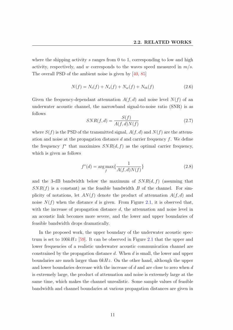
noise N(f) when the distance d is given. From Figure 2.1, it is observed that,
with the increase of propagation distance d, the attenuation and noise level in
an acoustic link becomes more severe, and the lower and upper boundaries of
feasible bandwidth drops dramatically.
In the proposed work, the upper boundary of the underwater acoustic spec-
trum is set to 100kHz [59]. It can be observed in Figure 2.1 that the upper and
lower frequencies of a realistic underwater acoustic communication channel are
constrained by the propagation distance d. When d is small, the lower and upper
boundaries are much larger than 0kHz. On the other hand, although the upper
and lower boundaries decrease with the increase of d and are close to zero when d
is extremely large, the product of attenuation and noise is extremely large at the
same time, which makes the channel unrealistic. Some sample values of feasible
bandwidth and channel boundaries at various propagation distances are given in
11

2. A REINFORCEMENT LEARNING BASED ENERGYEFFICIENT PROTOCOL FOR UA-WSNS AND ITSIMPLEMENTATION
0.5 1 1.5 2 2.5 30
10
20
30
40
50
60
Bou
ndar
ies
of fe
asib
le c
hann
el (k
Hz)
0.5 1 1.5 2 2.5 35
10
15
20
25
30
35
40
45
10lo
g 10[A
(f,d)
N(f)
] (dB
re µ
Pa2 /H
z)
Propagation Distance d (km)
Upper boundary of feasible channelLower boundary of feasible channel10log10[A(f,d)N(f)]
Figure 2.1: The lower and upper boundaries of an underwater acoustic communi-cation channel and the corresponding energy loss versus the propagation distance[59]
Table 2.1.
2.2.2 Q-Learning Algorithm
In underwater communication systems, the values of key decision variables for
the wireless sensor networks are difficult to be determined before deployments
due to the harsh environments. Therefore, model-free intelligent algorithms (e.g.
Q-Learning) can be used to optimize the system parameters according to the dy-
namic environments. In recent years, some underwater communication routing
protocols and energy-efficient schemes employed the reinforcement learning algo-
rithms [90, 91] to make the systems self-adaptive to the underwater environment.
Reinforcement Learning (RL) [82] is one of the well known artificial intelligence
algorithms that is capable of training an intelligent agent to interact with its en-
vironment so as to maximize the cumulative reward. In a reinforcement learning
12

2.2. RELATED WORKS
Table 2.1: The feasible bandwidth Btx(d), lower boundary fl(d) and upper bound-ary fu(d) corresponding to propagation distance d
d (km) Btx(d) (kHz) fl(d) (kHz) fu(d) (kHz)
0.1 39 19 580.2 34 16 500.3 30 15 450.4 28 13 410.5 26 12 380.6 24 12 360.7 23 11 340.8 22 10 320.9 21 10 311 21 9 30
framework, the interactions between an intelligent agent and the environment are
usually modeled as a markov decision process (MDP) [5, 35] which is the 4-tuple
(S, A, P, r) where S is a finite set of system states, A is the discrete and finite
action set, P is the collection of pa(s, s′) implying the probability that the system
transits from state s at time t to state s′ at time t+1 by taking action a, s, s′ ∈ S
and a ∈ A, and r indicates the instant reward the agent derived when system
state transits from s to s′ by taking action a [82]. In a markov decision process,
a policy π is defined as rule, by which the agent selects its action as a function
of states, i.e. the policy π : S × A → [0, 1] represents the probabilities of taking
action a when in state s. The value of state s under a policy π, denoted by v(s, π)
, is the expected reward of the agent in state s by following policy π,
v(s, π) =∞∑
t=0
γtEπ(r(st, at)|π, s0 = s) (2.9)
where s is a particular state, s0 indicates the initial state, r(st, at) is the reward
by taking action at at time t, γ ∈ [0, 1) is the discount factor, E(·) denotes the
expectation of (·). The solution to a MDP could then be treated as an optimal
policy π∗ maximizing the agent’s long-term reward [68].
A learning problem arises when the agent does not know the reward function
or the state transition probabilities. If an agent directly learns about its optimal
policy without knowing the reward function or the state transition function, such
13

2. A REINFORCEMENT LEARNING BASED ENERGYEFFICIENT PROTOCOL FOR UA-WSNS AND ITSIMPLEMENTATION
an approach is called model-free reinforcement learning, of which Q-Learning is
one example. The Q-Learning algorithm is one of the off-policy reinforcement
learning algorithms which enable the intelligent agent to update the estimated
value functions using the actions which have not actually been executed. In a
system with discrete and finite states and actions, the conventional Q-Learning
algorithms require the intelligent agent(s) to create and maintain a q-table in
which the state-action pairs and their corresponding q-values (i.e. the quality
values of the state-action pairs) are itemized. Whenever an action is to be deter-
mined at a state, the agent looks up the q-table and evaluates all feasible actions
at the current state. Then, the optimal action which maximizes the q-value is de-
termined and carried out. The corresponding quality value of that optimal action
is then updated to the maximum q-value. Many existing protocols and schemes
[8, 10, 15, 24, 61] have shown the effectiveness of the conventional Q-Learning
algorithm. The basic idea of Q-Learning is that we can define a function Q such
that
Q∗(s, a) = r(s, a) + γ∑
s′p(s′|s, a)v(s′, π∗) (2.10)
By this definition, Q∗(s, a) is the total discounted reward of taking action a in
state s and then following the optimal policy thereafter. By Equations (2.9) and
(2.10) we have
v∗(s, π∗) = maxa
Q∗(s, a) (2.11)
If we know Q∗(s, a) , then the optimal policy π∗ can be found by simply
identifying the action that maximizes Q∗(s, a) under state s. The problem is
then reduced to finding the function Q∗(s, a) instead of searching for the optimal
value of v∗(s, π∗). In [16], the update rule of Q values is given as follows,
Q(st, at) ← (1− αt)Q(st, at) + αt[r(st, at) + γ maxa′
Q(st+1, a′)] (2.12)
where the αt is the learning rate and satisfies∞∑
t=1
αt(st, at) = ∞ and∞∑
t=1
α2t (st, at) < ∞.
Then, the optimal action a∗t at state st is defined as the action maximizing the
14

2.3. SYSTEM DESCRIPTIONS
value of Q(st, at), as shown by the following equation,
a∗t = arg maxat∈Ast
Q(st, at) (2.13)
where the Ast is the set of feasible actions at state st . The procedure to implement
Q-Learning algorithm is summarized in the following [82]
Algorithm 1: Q-Learning algorithm description
Initializing the quality value Q(s, a) for all state-action pairs;Initializing state st at t = 0;for each iteration step t do
Evaluating the quality value for all feasible actions at st as follows;(1− αt)Q(st, at) + αt[r(st, at) + γ max
a′Q(st+1, a
′)];
Determining the optimal action a∗t achieving the max quality value atstate st using Equation (2.13);Update Q(st, a
∗t ) using Equation (2.12);
Carrying out a∗t and observing reward rt(st, a∗t ) and end state st+1;
st ← st+1;
2.3 System Descriptions
In this section, we employ the Q-Learning algorithm to model a distributed delay
tolerant UA-WSN. In the proposed system, a UA-WSN which consists of n static
sensor nodes anchored on the seabed and one mobile ferry node, is modeled as a
single agent Q-Learning system.
In the proposed system, the maximum transmission power of each sensor
node is constrained by the limited battery energy, which results in a relatively
small transmission range. As a result, the transmission areas of any two sensors
do not intersect. In other words, the sensors cannot communicate between each
other for exchanging information. Moreover, for the purpose of preserving energy,
each sensor node periodically transits between two operational states: active state
(high-power fully functional mode) and sleep state (low-power partially functional
mode) [46]. In the active state, the sensors are fully functional and are able
to transmit and receive, while in the sleep state, the sensors are just partially
15

2. A REINFORCEMENT LEARNING BASED ENERGYEFFICIENT PROTOCOL FOR UA-WSNS AND ITSIMPLEMENTATION
functional and cannot take part in the network activity. Each node (e.g. sensor
node i) switches to the active state according to a Poisson process with a rate
λi (in times/second). As a result, within a unit of time (i.e. one second), the
probability that node i switches to the active state for k times is expressed as
follows,
pi(k) = e−λiλki /k! (2.14)
The probability that sensor node i remains in the sleep status (i.e. k = 0) for
one second is
ps,i = pi(k = 0) = e−λi (2.15)
In either state, each sensor node keeps generating data packets at random
intervals and stores these packets in the local buffer as a first-in-first-out queue
with tail-drop. The destination of these outgoing packets may be any sensor node
except the ferry node and the generating node itself. Let G = g1, g2, · · · , gndenote the vector of generating rates of the n sensor nodes. The generating rates
may be different between nodes.
Compared with the sensor nodes, the ferry node is much more powerful in
terms of energy supply, storage space and computing capabilities. It is assumed
that the storage space and battery power of the ferry node are infinite. Moreover,
the ferry node is equipped with mobility and is able to continually travel around
the deployment area to collect/deliver data packets from/to sensors.
Additionally, it is assumed that there are a number of way-points in the
deployed area, each of which is defined as a specific position where the ferry node
can communicate with a specific sensor node(s). Obviously, a way-point must
be within the transmission range of at least one sensor node. Since there is no
intersection between the transmission areas of any two sensors, each sensor node
must have at least one unique way-point. The sensor i is the host node of way-
point wi. In the proposed system, we assume that each sensor node, e.g. node
i, has one, and only one, dedicated way-point denoted by wi, which is statically
located at the position of its host sensor.
The ferry node’s traveling route comprises a set of segments, each of which
connects two way-points. As a result, the path of the ferry node traversing the
transmission area of the targeting sensor is a folded line crossing the desired way-
16

2.3. SYSTEM DESCRIPTIONS
point. The traversing time Tv is defined as the time period that the ferry node
spends on the traversing path of a sensor node. Given a constant traveling speed
v of the ferry node, Tv = 2r/v where r is the radius of sensor node’s transmission
range. The ferry node has the freedom to determine the order of the way-points
it visits (i.e. dynamic traveling route). The speed and direction of the ferry node
are assumed to be unchanged between any two way-points (i.e. the ferry node
travels along a straight line between two way-points at a constant speed).
When travelling into the transmission range of a target sensor (the host sensor
of a specific way-point), the ferry node broadcasts beacon packets at a constant
rate to detect the presence of its target sensor node in the surrounding area.
Each active sensor node keeps listening to the underwater channel. If the beacon
packet is heard by the desired sensor which indicates that the ferry node has
traveled into the transmission range of this sensor node, an acknowledgement
packet is immediately generated by the sensor and sent back to the ferry node.
After receiving the acknowledgement packet, the ferry node looks up its local
buffer and delivers (uploads) the data packets targeting this sensor, and then
collects (downloads) all data packets from the sensor’s local buffer to the ferry
node. The upload and download processes are called a service.
Moreover, the traveling speed of the ferry node (0.5 ∼ 10m/s) is much slower
than the velocity of acoustic wave in underwater environment, and it is assumed
that the ferry node doesn’t stop its travel during services. In the proposed sys-
tem, sensor nodes exchange packets by the regular visiting of the ferry node. The
contacts between the ferry node and sensor nodes become critical since the suc-
cessful delivery of data packets totally depends on whether the ferry can contact
the sensor nodes during their active states. When arriving at a way-point, if the
ferry node cannot receive an acknowledgement from the host sensor, the ferry
node assumes that the host sensor is in the sleep state. In this situation, instead
of moving to the next way-point immediately, the ferry node stays at the current
way-point for a period which is the “waiting time” denoted by Tw to increase
the meeting probability with the specific sensor. During this period, the ferry
node keeps broadcasting beacon messages. If the sensor node enters the active
state before the end of the waiting period and responds to the ferry node, the
association between the ferry and sensor is established and a service starts. The
17
2. A REINFORCEMENT LEARNING BASED ENERGYEFFICIENT PROTOCOL FOR UA-WSNS AND ITSIMPLEMENTATION
ferry node keeps a record of the most recent time that it services the sensors, i.e.
Tr = tr1, tr2, · · · , trn.
2.3.1 System State Space
In the proposed system, the whole network is considered as a single agent Q-
Learning system [36]. The system states are discrete and related to the sensor
node which is being visited by the ferry node. In a network with n nodes, when
the ferry node arrives at the targeting sensor node j at time t, the system state
is defined as
st = j, j = 1, 2, . . . , n (2.16)
Therefore, the state space S which is defined as the collection of system states is
S = 1, 2, · · · , n.
2.3.2 Action Set
An action of the proposed system is defined as the ferry node’s visiting a specific
way-point. By carrying out an action at′ = i at time t′, the ferry travels to the
node i and the system state transits to st = i when the ferry node reaches the
way-point wi at time t. After servicing the sensor node i, the ferry node needs
to determine its next action (i.e. next way-point). The selection of the optimal
action depends on the evaluation of all feasible actions at the current state, i.e.
all the sensor nodes except current node i. Let Ai− = 1, · · · , i− 1, i + 1, · · · , ndenote the collection of sensors except node i, the action set at time t is defined
as At = Ai−.
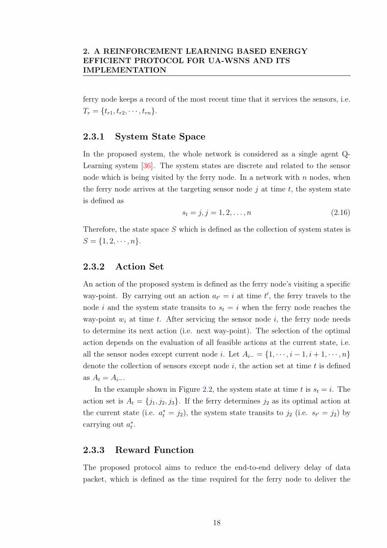
In the example shown in Figure 2.2, the system state at time t is st = i. The
action set is At = j1, j2, j3. If the ferry determines j2 as its optimal action at
the current state (i.e. a∗t = j2), the system state transits to j2 (i.e. st′ = j2) by
carrying out a∗t .
2.3.3 Reward Function
The proposed protocol aims to reduce the end-to-end delivery delay of data
packet, which is defined as the time required for the ferry node to deliver the
18

2.3. SYSTEM DESCRIPTIONS
Figure 2.2: System state and action set
packet from a given node (i.e. source) to a destination. In the design of reward
function, the main considerations include the ferry node’s traveling distance, the
sensor node’s queue length and the waiting time. Given the current state st = i
and action at = j, the ferry node’s current position is the same as the way-point
of sensor node i (i.e. wi) and the next way-point that the ferry node will visit is
wj corresponding to the host sensor node j. As a result, the reward is defined as
follows,
rij = dij + uij + qij (2.17)
where dij, uij and qij are obtained in the following.
1. Traveling Distance Factor: dij
When a ferry node travels between two way-points, longer distance between
the way-points causes longer traveling time which may result in generating
19

2. A REINFORCEMENT LEARNING BASED ENERGYEFFICIENT PROTOCOL FOR UA-WSNS AND ITSIMPLEMENTATION
and storing more data packets at all sensor nodes. For the purpose of
reducing the delivery delay and the number of packet drop, the ferry node
prefers to select the node at a relatively shorter traveling distance to visit.
Let d(wi, wj) denote the distance between the two way-points wi and wj.
Then the Traveling Distance Factor dij is defined as:
dij = −d(wi, wj)
dmax
(2.18)
where dmax is the maximum distance between any two way-points, i.e.
dmax = maxx,y=1,···,n
d(wx, wy). From (2.18), the lower d(wi, wj) is, the higher
value dij is, which indicates that short traveling distance deserves high re-
wards.
2. Waiting Time Factor: uij
In each visit, the meeting probability pm between the ferry node and a
sensor (e.g. sensor j) is dominated by the sleep probability of sensor j,
which can be expressed as follows
pm(j) = 1− (ps,j)Tv+Tw (2.19)
where ps,j is the probability that a sensor remains in its sleep state in a
unit time (i.e. one second), Tv and Tw are the traversing time and waiting
time, respectively. The probability that the sensor remains in the sleep
state within the ferry node’s traversing time is therefore (ps,j)Tv = e−Tvλj .
Thus the meeting probability during the traversing time between the ferry
node and the sensor node j is given as follows
pmt(j) = 1− e−Tvλj (2.20)
From (2.20), the meeting probability during traversing is a function of the
traversing period and λ.
Given a pre-specified minimum meeting probability pm, from (2.19) and
20

2.3. SYSTEM DESCRIPTIONS
(2.20), the length of a waiting period is estimated as follows
Tw,j =
0 if pmt(j) ≥ pm,
logps,j(1− pm)− Tv otherwise
(2.21)
Then the waiting time factor uij is defined as:
uij = − Tw,j
Tw,j,max
(2.22)
where Tw,j,max is the maximum waiting period which is defined as Tw,j,max =
logps(1− pm). From (2.22), the lower Tw,j is, the higher value uij is, which
indicates that short waiting period deserves high rewards.
3. Queue Length Factor: qij
The generated data packets are stored in each sensor node’s local buffer as
a first-in-first-out queue with tail-drop. Given node j’s generating rate gj,
the expected number of data packets generated between the ferry node’s
two successive visits is expressed as follows, shown as follows.
nj = gj(tnow − trj) + gjtij (2.23)
where tnow is current time, trj is the ferry node’s last visiting time to node
j, tij is the traveling time from current way-point (e.g. wi) to its potential
targets (e.g. wj), which is expressed as tij = d(wi, wj)/v where v is the
constant traveling speed of ferry and d(wi, wj) is the distance between the
way-points wi and wj. Given the maximum queue length qmax, the queue
length factor qij is defined as follows
qij =
1 if nj ≥ qmax,
nj
qmaxotherwise.
(2.24)
From (2.24), the lower nj is, the lower value qij is, which indicates that
short buffer queue deserves low rewards.
21

2. A REINFORCEMENT LEARNING BASED ENERGYEFFICIENT PROTOCOL FOR UA-WSNS AND ITSIMPLEMENTATION
2.4 Simulations
In this section, we apply the proposed Q-Learning based protocol to various
network topologies and use simulation results to demonstrate the effectiveness
and efficiency of our proposed protocol. The random-walk based data mules
protocol and the shortest-path based message ferry protocol are also implemented
as benchmarks. The detailed configurations and results of simulations are given
as follows.
2.4.1 Configurations
We consider a randomly generated network consisting of n = 20 nodes uniformly
and sparsely deployed over a 2000m× 2000m square area. The maximum trans-
mission range of sensor nodes is 50 meters. Each node independently generates
data packets according to a Poisson process with rate g packets/ second where
g ∈ [0.01, 0.05]. Note here that the generating rates may be different between
sensor nodes. The maximum length of buffer queue is 500 packets for all sensors.
The traveling speed of the ferry node varies from 0.5m/s to 10m/s in 0.5m/s
increments. The maximum waiting time for the proposed Q-Learning based pro-
tocol is set to be 5 seconds, but for the random-walk based and shortest-path
based protocols, the waiting time is set to be zero, i.e. the ferry node doesn’t
wait at the way-point when the response is not heard from the targeting sensor
node. The pre-specified meeting probability pm is set to be 0.8. The sleep/active
switching rate is set to be λ times/second where λ ∈ [0.005, 0.07]. In the Q-
Learning implementations, the discount factor γ = 0.5, and the learning rate
αt = 1/t, t = 1, 2, · · ·. The simulation results are shown in section 2.4.2. Each
simulation runs 5 × 10⁵ seconds and the simulation results are recorded. Each
data point is the average of twenty independent simulations.
2.4.2 Simulation Results
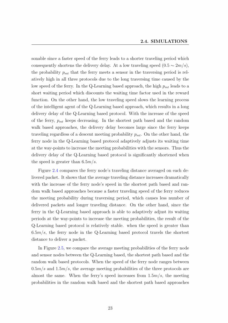
Figure 2.3 compares the average delivery delay among the three protocols. The
simulation result shows that the average delivery delay in all three protocols
decreases with the increase of the the ferry node’s speed. These results are rea-
22
2.4. SIMULATIONS
sonable since a faster speed of the ferry leads to a shorter traveling period which
consequently shortens the delivery delay. At a low traveling speed (0.5 ∼ 2m/s),
the probability pmt that the ferry meets a sensor in the traversing period is rel-
atively high in all three protocols due to the long traversing time caused by the
low speed of the ferry. In the Q-Learning based approach, the high pmt leads to a
short waiting period which discounts the waiting time factor used in the reward
function. On the other hand, the low traveling speed slows the learning process
of the intelligent agent of the Q-Learning based approach, which results in a long
delivery delay of the Q-Learning based protocol. With the increase of the speed
of the ferry, pmt keeps decreasing. In the shortest path based and the random
walk based approaches, the delivery delay becomes large since the ferry keeps
traveling regardless of a descent meeting probability pmt. On the other hand, the
ferry node in the Q-Learning based protocol adaptively adjusts its waiting time
at the way-points to increase the meeting probabilities with the sensors. Thus the
delivery delay of the Q-Learning based protocol is significantly shortened when
the speed is greater than 6.5m/s.
Figure 2.4 compares the ferry node’s traveling distance averaged on each de-
livered packet. It shows that the average traveling distance increases dramatically
with the increase of the ferry node’s speed in the shortest path based and ran-
dom walk based approaches because a faster traveling speed of the ferry reduces
the meeting probability during traversing period, which causes less number of
delivered packets and longer traveling distance. On the other hand, since the
ferry in the Q-Learning based approach is able to adaptively adjust its waiting
periods at the way-points to increase the meeting probabilities, the result of the
Q-Learning based protocol is relatively stable. when the speed is greater than
6.5m/s, the ferry node in the Q-Learning based protocol travels the shortest
distance to deliver a packet.
In Figure 2.5, we compare the average meeting probabilities of the ferry node
and sensor nodes between the Q-Learning based, the shortest path based and the
random walk based protocols. When the speed of the ferry node ranges between
0.5m/s and 1.5m/s, the average meeting probabilities of the three protocols are
almost the same. When the ferry’s speed increases from 1.5m/s, the meeting
probabilities in the random walk based and the shortest path based approaches
23

2. A REINFORCEMENT LEARNING BASED ENERGYEFFICIENT PROTOCOL FOR UA-WSNS AND ITSIMPLEMENTATION
0 2 4 6 8 100
1
2
3
4
5
6x 10⁴
speed of ferry node (m/s)
aver
age
deliv
ery
dela
y (s
econ
ds)
Random Walk BasedShortest Path BasedQ−Learning Based
Figure 2.3: delivery delay versus speed of ferry node
0 2 4 6 8 100
5
10
15
20
25
30
35
40
speed of ferry node (m/s)
trave
ling
dist
ance
of f
erry
per
del
iver
ed p
acke
t
Random Walk BasedShortest Path BasedQ−Learning Based
Figure 2.4: Ferry node’s traveling distance per delivered packet versus speed offerry node
24

2.5. CONCLUSION
dramatically decrease due to the shorter traversing time caused by the faster
speed of the ferry. On the other hand, the average meeting probability in the
Q-Learning based protocol outperforms the other two protocols and converges to
0.8 which is a pre-specified meeting probability. This result is consistent with
Figure 2.4.
Figure 2.6 compares the variance of meeting probabilities among these three
protocols. It shows that the variance of the meeting probabilities of the Q-
Learning based protocol is much lower than that of the random walk based and
the shortest path based approaches. When the speed of the ferry node increases
from 1.5m/s, the variance decreases dramatically and remains stable, which is
consistent with Figure 2.5 where the average meeting probabilities comparisons
are shown. The Q-Learning based approach enables the ferry node to adaptively
adjust its waiting time at way-points and the order of its visits so that the meeting
probabilities of the ferry node and sensors distribute evenly across the network,
which leads to a low variance.
2.5 Conclusion
Current researches on DTNs rely on increasing the meeting probabilities of sen-
sors, which are important for keeping a good throughput and a relatively short
delivery delay. In underwater acoustic wireless sensor networks (UA-WSNs), this
problem becomes challenging due to the unique properties of underwater envi-
ronments. In this chapter we proposed a Q-Learning based protocol which is
used to reduce the delivery delay and delivery cost by maximizing the meeting
probabilities between the ferry node and the sensor nodes. Through simulations,
we have demonstrated the feasibility and efficiency of the protocol in UA-WSNs.
25

2. A REINFORCEMENT LEARNING BASED ENERGYEFFICIENT PROTOCOL FOR UA-WSNS AND ITSIMPLEMENTATION
0 2 4 6 8 10
0.4
0.5
0.6
0.7
0.8
0.9
1
speed of ferry node (m/s)
aver
age
mee
ting
prob
abili
ties
Random Walk BasedShortest Path BasedQ−Learning Based
Figure 2.5: Average meeting probabilities versus speed of ferry node
0 2 4 6 8 100
0.005
0.01
0.015
0.02
0.025
0.03
0.035
0.04
0.045
0.05
speed of ferry node (m/s)
varia
nce
of m
eetin
g pr
obab
ilitie
s
Random Walk BasedShortest Path BasedQ−Learning Based
Figure 2.6: Variance of meeting probability versus speed of ferry node
26

Chapter 3
A Neural-Q-Learning Based
Approach for Delay Tolerant
Underwater Wireless Sensor
Networks
3.1 Introduction
In underwater communication systems, the values of key decision variables for the
wireless sensor networks are difficult to be determined before deployments due
to the harsh and dynamic environments. Therefore, many intelligent algorithms
(e.g. Q-Learning) are employed to optimize the system parameters according
to the environment. In recent years, many underwater communication routing
protocols and energy-efficient schemes [18, 36, 37, 57, 70, 89] employed the Q-
Learning algorithm which is one of the widely used machine learning algorithms
to make the systems self-adaptive to the environment. The intelligent agent
of a conventional Q-Learning system with discrete state space and action set
creates and maintains a lookup table (named q-table) to store the state-action
pairs and their corresponding q-values (i.e. quality values of the state-action
pairs). Whenever an action is to be determined at a state, the agent looks up
the q-table to evaluate and compare the quality values of all feasible actions at
27

3. A NEURAL-Q-LEARNING BASED APPROACH FOR DELAYTOLERANT UNDERWATER WIRELESS SENSOR NETWORKS
the given state. The optimal action which achieves the highest quality value is
then determined and carried out by the agent. Correspondingly, the q-value of the
optimal action is updated to the maximum quality value. In recent decades, many
existing protocols and schemes have shown the effectiveness of the conventional
Q-Learning algorithms. However, these algorithms become inefficient when the
number of the feasible actions (i.e. the entries of state-action pairs in the q-
table) is large since the agent has to evaluate and compare the quality value of
all the actions to determine the optimal one, or even infeasible if the action set
is continuous (i.e. infinite entries in the q-table) [9, 21, 51, 84]. As a result, it is
necessary to develop an effective and efficient method to determine the optimal
action in a large, or even continuous, action set at a given system state.
In this chapter, we propose a Neural-Q-Learning (NQL) [26, 39] based delay-
tolerant protocol for underwater acoustic wireless sensor networks (UA-WSNs).
The proposed NQL protocol reduces the delivery delay by enabling the ferry (i.e.
the NQL agent) to find an efficient and relatively short traveling route which
inter-connects the optimized way-points to deliver data packets between sensors.
The optimal position of the way-points which are dynamic in a two-dimensional
continuous space is determined by the ferry based on its independent learning
from the environment. Compared with the conventional Q-Learning algorithms,
the NQL agent avoids searching a large or infinite lookup table. More specifically,
a delay-tolerant underwater acoustic wireless sensor network (UA-WSN) is mod-
eled as a single agent NQL system [26, 38, 39, 58], in which an artificial neural
network (ANN) along with a wire-fitting interpolator are employed to produce
a continuous q-curve to replace the discrete q-table used in the conventional Q-
Learning algorithms. At a given state, the ANN first reads in the system state as
input parameter and outputs a fixed number of samples (known as “control wires”
or “wires” in short), each of which consists of an action and the corresponding
quality value of the action at the given state. Then, the wire-fitting interpolator
uses these wires to fit a continuous curve which describes the relationship of the
quality value and the action in a continuous manner. By adopting the q-curve,
the agent is capable of effectively and efficiently determining the optimal action
which achieves the greatest function value(s) of the q-curve. Since the perfor-
mance of the proposed system greatly depends on the q-curve, it is necessary to
28

3.1. INTRODUCTION
keep improving the performance of the ANN and the wire-fitting interpolator to
produce accurate q-curves. Once an optimal action is determined and carried
out, the agent evaluates the instant reward/penalty obtained from the environ-
ment, and calculates a practical quality value which is then used to reposition
the existing wires. The repositioned wires are used not only by the wire-fitting
interpolator to re-generate the q-curve, but also to train the ANN to improve the
accuracy of the produced wires.
In the proposed delay tolerant UA-WSN, the network consists of a mobile ferry
node and a number of static sensors. The sensors are assumed to be sparsely-
distributed, energy-constrained, stationary, and consequently are not capable of
peer to peer sensor communications. Thus a ferry is employed to travel around
the deployment field to collect, carry and deliver data packets between sensors.
A specific position where the ferry contacts with a specific sensor is known as a
way-point. The traveling route of the ferry consists of a number of segments, each
of which connects two way-points. The ferry has the freedom to determine the
position and the order of the way-points to be visited according to its independent
learning. The state of the NQL system is presented by the index number of the
sensor which is being visited by the ferry at the given time instant. The action
of the intelligent agent is defined as a specific way-point which is to be visited
by the ferry. Since the position of a way-point is not fixed and can be arbitrary
within the transmission range of its host sensor, the action set is a continuous
two-dimensional space. Whenever an optimal action (i.e. the optimal position of
a way-point to be visited by the ferry) is to be determined, the ferry selects the
optimal way-point which achieves the greatest function value(s) of the q-curve.
Simulation results show that the NQL system improves the system performance
by maximizing the meeting probabilities between the ferry and the sensors on the
optimized traveling route.
The rest of this chapter is organized as follows. In section 3.2, the artificial
neural network is briefly reviewed, followed by the introduction of the Neural-Q-
Learning algorithm. The detailed implementations of the proposed system are
described in section 3.3. Then, simulation configurations and results are given in
section 3.4. Finally, the conclusion is drawn in section 3.5.
29
3. A NEURAL-Q-LEARNING BASED APPROACH FOR DELAYTOLERANT UNDERWATER WIRELESS SENSOR NETWORKS
3.2 Related Work
In a markov decision process system with discrete and finite states and actions,
the conventional Q-Learning algorithms require the intelligent agent(s) to create
and maintain a q-table in which the state-action pairs and their corresponding
q-values (i.e. the quality values of the state-action pairs) are itemized. Whenever
an action is to be determined at a state, the agent looks up the q-table and
evaluates all feasible actions at the current state. Then, the optimal action which
maximizes the q-value is determined and carried out. The corresponding quality
value of that optimal action is then updated to the maximum q-value. Many
existing protocols and schemes have shown the effectiveness of the conventional
Q-Learning algorithm. However, the conventional Q-Learning algorithm becomes
inefficient when the number of feasible actions (i.e. the entries of state-action
pairs in the q-table) is large since the agent has to evaluate and compare each
of them to determine the optimal action. If the action set is continuous, the
look-up process of the conventional Q-Learning algorithms will be infeasible. As
a result, it is necessary to develop an effective and efficient method to determine
the optimal action in a large, or even continuous, action set at a state.
In this chapter, the proposed system with a continuous action set employs
a Neural-Q-Learning approach to determine the optimal position of way-points
in a two-dimensional continuous space. These optimized way-points lead to an
efficient traveling route to reduce the delivery delay and delivery cost. The related
works are briefly reviewed in this section. More specifically, the conventional Q-
Learning algorithms, the neural network and the Neural-Q-Learning algorithm
are introduced.
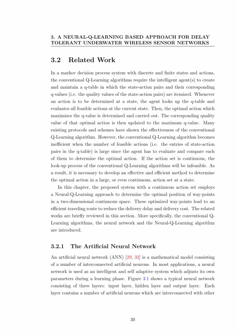
3.2.1 The Artificial Neural Network
An artificial neural network (ANN) [29, 32] is a mathematical model consisting
of a number of interconnected artificial neurons. In most applications, a neural
network is used as an intelligent and self adaptive system which adjusts its own
parameters during a learning phase. Figure 3.1 shows a typical neural network
consisting of three layers: input layer, hidden layer and output layer. Each
layer contains a number of artificial neurons which are interconnected with other
30

3.2. RELATED WORK
neurons on the adjacent layers. Each artificial neuron has an activation function,
f(x), which maps the input, x, to the neuron’s output. The activation function
of different neurons may be different, but in most cases, the neurons in the same
layer employ identical activation functions. Nowadays, the most commonly used
activation functions consists of the log-sigmoid function, tan-sigmoid function and
the linear combination function [94]. On the other hand, given a fixed number
of neurons, the structure of the ANN is determined by the connections (links)
between neurons. Each link connects two neurons and is assigned a weighting
coefficient to indicate the importance of the link, e.g. uij indicates the weighting
coefficient of the link connecting neurons i and j. The output yi is weighted by
multiplying the weighting coefficient uij before feeding into neuron j. If there is
more than one input link connecting to neuron j, the input value of neuron j’s
activation function is the weighted sum of all the input links, i.e. xj =∑
k∈K
ykukj
where K is the set of the neurons feeding input value to the neuron j. If the
structure of the ANN is directed acyclic, the system is known as a feed-forward
ANN [34], otherwise the networks with cycles are commonly called recurrent [19].
3.2.2 The Neural-Q-Learning Algorithm
The artificial neural network based Neural-Q-Learning algorithm was first intro-
duced in [86]. In the NQL algorithm, the action set is assumed to be continuous
at a given state which is discrete and finite. A continuous q-curve explicitly
describing the relationship between the action and the corresponding q-value is
introduced to replace the q-table used in the conventional Q-Learning algorithms.
The agent of NQL determines the optimal action by searching the action that
maximizes the q-value in the q-curve. This approach improves the efficiency of the
Q-Learning algorithm in a system with a large action set by avoiding searching
through a large lookup table.
The effectiveness of the proposed NQL system greatly depends on the q-
curve generated by an approximation method which is known as the wire-fitting
technique [86]. The wire-fitting technique consists of an ANN algorithm and a
moving least square (MLS) interpolation method [22, 52]. Initially, by reading
31

3. A NEURAL-Q-LEARNING BASED APPROACH FOR DELAYTOLERANT UNDERWATER WIRELESS SENSOR NETWORKS
Figure 3.1: A three-layer artificial neural network
the system state as the input parameter, the ANN outputs a number of actions
along with their corresponding q-values. Each action and its quality value at the
given state are named a “wire”. Note that, given a fixed structure for the ANN,
the number of output wires remains unchanged. Then, a moving least square
method is employed to interpolate these wires and fit a continuous q-curve. Once
the q-curve of a given state is generated, the NQL agent then determines the
optimal action by searching for the maximum values of the q-curve. By carrying
out the optimal action at a given state, the system transits to its next state.
Moreover, the efficiency of NQL systems can be improved by using a q-curve
with high accuracy which relies on the wires generated by the ANN, thus we
employ the back-propagation method [69] to train the ANN to produce the wires
with high accuracy. After carrying out an optimal action a at a given state s, the
system transits to its next state s′ and the NQL agent obtains an instant reward
r(s, a) from the environment. Accordingly, a practical quality value Q(s, a) of
32

3.3. SYSTEM DESCRIPTION
action a at state s can be evaluated as follows.
Q(s, a) ← (1− αt)Q(s, a) + αt[r(s, a) + γ maxa′
Q(s′, a′)] (3.1)
where γ is the discount factor and αt is the learning rate which satisfies∞∑
t=1
αt = ∞
and∞∑
t=1
α2t < ∞. This practical quality value is more accurate than the one ap-
proximated by ANN and the wire-fitting interpolator. Consequently, based on
the practical q-value along with the selected optimal action a, the agent uses the
gradient-descent method (the partial derivative method) [26] to reposition the
existing wires. The repositioned wires are then used (as the desired output) to
train the ANN with back propagation method [33, 44, 69] so as to improve the
accuracy of the future approximations of ANN. Also, these repositioned wires are
used by the wire-fitting interpolator to generate a new q-curve. Figure 3.2 shows
the flow chart of the neural Q-Learning algorithm.
3.3 System Description
In this section, we describe the proposed Neural-Q-Learning (NQL) algorithm
as applied in a distributed delay tolerant UA-WSN. In the proposed system, a
UA-WSN consisting of m static sensors and one mobile ferry is modeled as a
single agent NQL system.
Due to the constrained battery power, the transmission range of each sensor is
very limited. As a result, the transmission area of any two sensors does not overlap
and the sensors cannot communicate with each other for exchanging information.
Moreover, for the purpose of conserving energy, each sensor periodically transits
between two operational states: the active state (high-power fully functional
mode) and the sleep state (low-power partially functional mode). In the active
state, the sensor is fully functional and is able to transmit and receive, while in
the sleep state the sensor cannot take part in the network activity. Each sensor
switches to the active state according to a Poisson process with a rate λ (in
times/second). Within a unit of time (i.e. one second), the probability that the
sensor switches to the active state for k times is expressed as p(k) = e−λλk/k!. As
33

3. A NEURAL-Q-LEARNING BASED APPROACH FOR DELAYTOLERANT UNDERWATER WIRELESS SENSOR NETWORKS
!" "#$%#& '#%
(" (" %%($)"%'!( (%! *+",, "(
Figure 3.2: Flow chart of the neural Q-learning algorithm
a result, the probability of that sensor remaining in the sleep state (i.e. k = 0) in
one second is ps = p(k = 0) = e−λ. In either state, each sensor keeps generating
data packets at random intervals (i.e. according to environmental phenomenon)
and stores these packets in the local buffer as a first-in-first-out queue with tail-
drop. Note here that the generating rates may be different among sensors.
Compared with the sensors, the ferry is much more powerful in terms of en-
ergy supply, storage space and computing capacities. Thus, we assume that the
storage space of the ferry is infinite. On the other hand, the ferry is equipped
with mobility and is capable of continually traveling around the deployment area
to collect/deliver data packets from/to sensors. The traveling route of the ferry
comprises a set of segments. Each of these segments connects two way-points,
34

3.3. SYSTEM DESCRIPTION
each of which is defined as a specific position where the ferry can communicate
with a certain sensor. Obviously, a way-point must be within the transmission
range of at least one sensor. Since there is no intersection between the trans-
mission areas of any two sensors, each sensor, e.g. sensor i, must have a unique
and dedicated way-point denoted by wi. The sensor i is known as the host sen-
sor of wi. Note here that the positions of way-points are dynamic within the
transmission range of their host sensors and are determined by the ferry. We also
assume that the speed and direction of the ferry do not change when traveling
between any two way-points (i.e. the ferry travels along a straight line between
two way-points at a constant speed). When traveling into the transmission range
of a target sensor (the host sensor of a specific way-point), the ferry broadcasts
beacon packets at a constant rate to detect the presence of its target sensor in
the surrounding area. All the sensors keep listening to the underwater channel. If
the beacon packet is received by the desired sensor, an acknowledgement packet
is generated by the sensor and sent to the ferry immediately. After receiving
the acknowledgement packet, the ferry looks up its local buffer and transmits
(uploads) the data packets targeting to this sensor and collects (downloads) all
the data packets from this sensor’s local buffer. The upload and download pro-
cess is known as a service. The traveling speed of the ferry (0.5 ∼ 10m/s [7])
is much slower than the propagation speed of acoustic wave in the underwater
environment (1500m/s [85]), thus it is assumed that the ferry doesn’t stop its
travel during services.
3.3.1 Neural-Q-Learning Framework
3.3.1.1 System State Space
In the proposed system, the whole network is considered as a single agent Neural-
Q-Learning system [26]. The system states are discrete and related to the sensors
that the ferry visits. For instance, when the ferry is visiting and servicing sensor
i at time t, the system state is defined as st = i. Consequently, the system state
space denoted by S is discrete and finite, i.e. S = 1, 2, · · · ,m.
35

3. A NEURAL-Q-LEARNING BASED APPROACH FOR DELAYTOLERANT UNDERWATER WIRELESS SENSOR NETWORKS
3.3.1.2 Optimal Action and Action Set
An action a of the NQL agent is defined as a specific way-point that the ferry
targets to visit. For instance, after servicing sensor i at time t (i.e. st = i), the
action of the ferry is to travel to the next way-point to service the host sensor of
that way-point. Since sensor i has been serviced, both the ferry and the sensor i
do not have buffered packet to exchange. As a result, sensor i is excluded from
the set of sensors to be serviced. Thus the action set at time t is defined as
At =⋃
k∈i−Rk where i− = 1, · · · , i − 1, i + 1, · · · ,m and Rk is the transmission
area of sensor k. Let wj denote the selected target way-point, the action at time t
is defined as at = wj, where wj ∈⋃
k∈i−Rk and at ∈ At. Apparently, the action set
At is continuous due to the continuity of the transmission area R of each sensor.
The target of the agent is to determine the optimal position of way-points,
which achieves the maximum quality value. At a given state, e.g. st = i, the
highest quality value q∗t that the ferry can achieve is
q∗t = maxk∈i−
q∗t (k) = maxq∗t (1), · · · , q∗t (i− 1), q∗t (i + 1), · · · , q∗t (m) (3.2)
where q∗t (k) = Q(st, a∗tk) and a∗tk = arg max
atk∈Rk
Q(st, atk). Correspondingly, the tar-
get sensor to be visited by the ferry is sensor j where j = arg maxk∈i−
q∗t (k) and the
optimal action (i.e. the optimal position of the way-point of the target sensor j)
is a∗t = a∗tj = arg maxatj∈Rj
Q(st, atj).
In the example shown in Figure 3.3, the system state at time t is st = i. The
shadowed area indicates the action set At =⋃
k∈i−Rk = Rj1 ∪ Rj2 ∪ Rj3 which is
the union of the three shaded circles. If the ferry determines wj2 as its optimal
action at the current state (i.e. a∗t = wj2), the system state transits to j2 (i.e.
st′ = j2) by carrying out a∗t .
Furthermore, by using polar coordinates, the position of a way-point wi rela-
tive to its host sensor (e.g. the sensor i ) can be represented by (θwi, rwi
)i where
θwiand rwi
are the angle and distance of the way-point wi relative to the position
of its host sensor i. In other words, an action a is interpreted as the polar coor-
dinates of the way-point wi, i.e. a = (θwi, rwi
)i, where θwi∈ [0, 2π], rwi
∈ [0, r]
36

3.3. SYSTEM DESCRIPTION
Figure 3.3: System state and action set
and r is the maximum transmission range of the sensor. Given xi and yi as the
coordinates of the sensor i, the coordinates of the way-point wi are given by
xwi= xi + rwi
cos(θwi) and ywi
= yi + rwisin(θwi
), as shown in Figure 3.4.
3.3.2 Generating the Q-Curve
Differing from the conventional Q-Learning algorithms, the proposed NQL sys-
tem approximates the optimal action by searching the maximum value(s) of a
continuous q-curve which is produced by an ANN along with a wire-fitting inter-
polator. The ANN is used to generate a fixed number of discrete samples (known
as control wires) which are then used in the wire-fitting interpolator to fit a con-
tinuous q-curve. In this section, the implementation details of both techniques
are depicted.
37

3. A NEURAL-Q-LEARNING BASED APPROACH FOR DELAYTOLERANT UNDERWATER WIRELESS SENSOR NETWORKS
Figure 3.4: The polar coordinates of a way-point relative to its host sensor
3.3.2.1 The ANN Implementation
The proposed Neural-Q-Learning system [86] employs the Artificial Neural Net-
work (ANN) technique to produce a fixed number of discrete wires, each of which
represents an action and the corresponding quality value of the action at the given
state. The ANN used in the system has a typical fully connected feed-forward
structure [3, 62] which consists of an input layer, a hidden layer and an output
layer.
The coordinates of the ferry’s position denoted by xf and yf are used as the
input parameters to the ANN. As a result, there are only two neurons in the
input layer. In the output layer, the neurons produce the elements for the control
wires. Let Ω = ω1, · · · , ωN denote the collection of the produced N wires
where ωk is the k-th wire. Each wire is a 3-tuple consisting of ζθ, ζr and ζq which
correspond to the polar coordinates (θwi,rwi
)i of a specific way-point wi and its
corresponding quality value qwi. Therefore, the ANN needs 3N neurons in the
output layer to produce the N wires. Furthermore, the log-sigmoid functions are
38

3.3. SYSTEM DESCRIPTION
Figure 3.5: The structure of ANN employed in the proposed system
used at the output neurons to limit the magnitude of all outputs between 0 and
1, i.e. ζθ, ζr, ζq ∈ [0, 1]. Figure 3.5 describes the detailed structure of the ANN
employed in the proposed system. For a given wire ωk = (ζθk, ζrk, ζqk) where
k ∈ [1, N ], the corresponding polar coordinates of the way-point and its quality
value are given by θwi= 2πζθk, rwi
= rζrk, and qwi= qinit + ∆q where qinit is
the initial quality value, ∆q = C · (2ζqk − 1) and C is a constant. Note here that
the change of a quality value, i.e. ∆q, may be positive or negative. As a result,
the factor ζq which is the output of a log-sigmoid function and ranges between
0 and 1 is converted into (2ζq − 1) ∈ [−1, 1] so that ∆q ∈ [−C, C]. The hidden
layer consists of a fixed number of neurons (known as “hidden neurons” [3]), each
of which is interconnected with other neurons in the input and output layers.
The log-sigmoid functions are employed by the hidden neurons as the activation
functions.
39

3. A NEURAL-Q-LEARNING BASED APPROACH FOR DELAYTOLERANT UNDERWATER WIRELESS SENSOR NETWORKS
3.3.2.2 The Wire-Fitting Function
Once the discrete wires are produced, a wire-fitting function defined by a moving
least square (MLS) interpolation [52] is found by fitting a continuous curve (or
surface) to the wires. In the proposed approach, the wire-fitting interpolator is
employed to find a continuous function ζq(σa) by using the N wires produced by
the ANN as follows,
ζq(σa) =
N∑k=1
ζqk[||σa − σak||2 + c(ζq,max − ζqk) + ε]−1
N∑k=1
[||σa − σak||2 + c(ζq,max − ζqk) + ε]−1
(3.3)
where σa = (ζθ, ζr), σak = (ζθk, ζrk), ζq,max = maxk∈[1,N ]
ζqk, c is a small smoothing
factor and ε is a small positive constant [26, 39].
With a determined function ζq(σa), the maximum function value(s) ζ∗q and
the corresponding σ∗a = (ζ∗θ , ζ∗r ) which achieves ζ∗q can be determined. Thus the
optimal action which achieves the highest quality value q∗wi= qinit + C · (2ζ∗q − 1)
is a∗ = (θ∗wi, r∗wi
)i where θ∗wi= 2πζ∗θ and r∗wi
= rζ∗r .
3.3.3 Improvement of the ANN and the Q-Curve
The selection of the optimal way-points relies on the q-curve. Thus it is desirable
to improve its accuracy. In this section, we describe the details of the training of
the ANN and the adjustments of the q-curve by using a practical quality value.
3.3.3.1 Evaluation of the Practical Quality Value
Once an optimal action a∗ (i.e. an optimal way-point) is determined and carried
out by the agent at state s, the ferry moves to the selected way-point and the
system transits to a new state s′. By taking this action, the agent derives the
instant reward/penalty r(s, a∗) from the environment accordingly. Based on these
parameters, a practical quality value denoted by Q(s, a∗) is evaluated using (3.1).
Note here that, differing from the conventional Q-Leaning algorithms where the
quality value is evaluated before the execution of an action, the NQL system
calculates Q(s, a∗) after the optimal action having been carried out. Thus r(s, a∗)
40

3.3. SYSTEM DESCRIPTION
and maxa′
Q(s′, a′) used in (3.1) are online and actual values. As a result, the
evaluated practical quality value represents the actual quality of the selected
action a∗ at state s, which deserves a higher accuracy than the estimated quality
values of the conventional Q-Leaning algorithms.
In the evaluation of the practical quality value, the reward function plays an
important role as it determines the behavior of the NQL agent in the long term.
For our proposed approach, the main considerations in the design of the reward
function include the ferry’s traveling distance, the ferry’s waiting time at a way-
point, the effective bandwidth, the target sensor’s queue length and the contact
between the ferry and the target sensor. Given st = i and at = wj, the reward
function is defined as
r(st, at) = uj · (dij + bj + tj + qj) (3.4)
where uj is set to 1 if the ferry services sensor j successfully, or 0 otherwise, dij,
bj, tj and qj are obtained in the following.
1. Traveling Distance Factor: dij
When a ferry travels towards a way-point at a constant traveling speed, a
long traveling distance causes a long traveling time which results in not only
an increase of the delivery delay, but also a large number of data packets
being generated and stored at all sensors. For the purpose of reducing the
packet delivery delay and the number of buffered packets, the ferry prefers
to select the sensor which is located at a relatively short traveling distance
to visit. Let d(wi, wj) denote the distance between two way-points wi and
wj, then the traveling distance factor dij is defined as:
dij =dmax − d(wi, wj)
dmax
(3.5)
where dmax = maxx,y=1,···,m
d(x, y) + 2r is the maximum distance between
any two way-points and r is the transmission range of the sensors. (3.5)
indicates that a short traveling distance deserves a high reward.
2. Effective Bandwidth Factor: bj
41

3. A NEURAL-Q-LEARNING BASED APPROACH FOR DELAYTOLERANT UNDERWATER WIRELESS SENSOR NETWORKS
The effective bandwidth of an underwater acoustic channel is dominated
by the distance between the transmission peers. The shorter the distance
is, the larger the effective bandwidth is. Apparently, the ferry prefers a
larger bandwidth to exchange data packets efficiently. Thus, the effective
bandwidth factor bj is defined as:
bj =Bwj ,j
Bmax
(3.6)
where Bmax is the maximum bandwidth of the entire spectrum of the under-
water acoustic channel and Bwj ,j is the effective bandwidth of the acoustic
communication channel between the way-point wj and its host sensor j.
Bwj ,j is determined according to the distance between wj and j, as shown
in Figure 2.1 and Table 2.1. Note that the position of wj is determined by
the ferry and must be located in the transmission range of sensor j. (3.6)
implies that a large bandwidth results in a high reward.
3. Waiting Time Factor: tj
If the ferry does not meet the desired target sensor, it has to wait at the
way-point until the sensor is activated or a maximum waiting time denoted
by Tw is reached. The sleep probability of the sensor dominates the length
of the waiting time and the meeting probability pm between the ferry and
its target sensor. pm can be calculated by pm = 1 − (ps)tv+tw where ps
is the probability that the sensor remains in its sleep state in a unit time
(i.e. one second), tv and tw are the traversing time and waiting time of
the ferry, respectively. Given a pre-specified maximum meeting probability
pm,max between the ferry and the desired sensor, the maximum waiting time
is determined as Tw = logps(1 − pm,max). Thus, for a specific sensor j, the
waiting time factor tj is defined as:
tj =Tw − twj
Tw
(3.7)
where twjis the actual waiting time that the ferry spends at the selected
way-point wj. (3.7) indicates that a short waiting time leads to a high
reward.
42

3.3. SYSTEM DESCRIPTION
4. Queue Length Factor: qj
In the proposed system, the generated data packets are stored in each sen-
sor’s local buffer as a first-in-first-out queue with tail-drop. If the buffer of a
sensor is full, the incoming packets are dropped at the sensor. To reduce the
number of dropped packets, the sensor with a relatively large buffer queue
should have a high priority to be serviced by the ferry. Consequently, the
queue length factor qj of sensor j is calculated as follows
qj =nj
qmax
(3.8)
where nj is the number of data packets collected by the ferry at sensor j
and qmax is the maximum capacity of the buffer queue. (3.8) indicates that
a small buffer queue deserves a low reward.
3.3.3.2 Repositioning Wires with Gradient-Descent Method
After an optimal action a∗ is carried out at a given state s, the agent evaluates
the practical quality value Q(s, a∗) which is then converted into a ζ∗q factor by
ζ∗q = (Q(s,a∗)−qinit
C+ 1)/2. Combining with the ζ∗θ and ζ∗r factors corresponding to
the optimal action a∗, a practical wire ω is generated i.e. ω = (ζ∗θ , ζ∗r , ζ∗q ). The
practical wire is used to reposition the existing N wires by the gradient-descent
method [6, 26, 56]. The displacements of the k-th wire are ∆ζqk =∂ζq(σa)
∂ζqk∆qk,
∆ζθk =∂ζq(σa)
∂ζθk∆qk and ∆ζrk =
∂ζq(σa)
∂ζrk∆qk, where ∆qk = ζ∗q − ζqk. Let D(σa) =
||σa − σak||2 + c(ζq,max − ζqk) + ε, N(σa) =k∑
i=1
1D(σa)
and W (σa) =k∑
i=1
ζqk
D(σa),
respectively, the partial derivative terms∂ζq(σa)
∂(·) are given as follows.
∂ζq(σa)
∂ζqk=
[D(σa)+ζqk·c]·N(σa)−W (σa)·cN2(σa)·D2(σa)
∂ζq(σa)
∂ζθk=
[ζθk·N(σa)−W (σa)]·2(σa−σak)
N2(σa)D2(σa)∂ζq(σa)
∂ζrk=
[ζrk·N(σa)−W (σa)]·2(σa−σak)
N2(σa)D2(σa)
(3.9)
Consequently, the k-th wire is repositioned to (ζθk + ∆ζθk, ζrk + ∆ζrk, ζqk +
∆ζqk). By repositioning all the N wires and using the same wire-fitting function
introduced in section 3.3.2.2, a new continuous q-curve is generated.
43

3. A NEURAL-Q-LEARNING BASED APPROACH FOR DELAYTOLERANT UNDERWATER WIRELESS SENSOR NETWORKS
3.3.3.3 Training ANN with Back Propagation
Besides being used to re-generate the q-curve, the repositioned wires are also
employed to train the ANN. The production of the wires depends on the input
parameters and the structure of the ANN. Given a fixed structure of the ANN,
the objective of training the ANN is to adjust the weights of connections between
neurons so that it is capable of producing the wires with high accuracy. In the
training process of the ANN, the weight coefficient of each link connecting two
neurons can be tuned by the back propagation technique [69]. In our proposed
approach, the back propagation technique uses the repositioned wires as the de-
sired output set to generate the deltas of all neurons at the output layer and
the hidden layer. The propagated errors are then used to calculate the gradient
of the weights which determines how to adjust the weights [69]. A fully trained
ANN that reaches its stable state is capable of minimizing the errors between its
outputs and the provided samples, i.e. the repositioned wires.
Note here that the generation of a continuous q-curve, i.e. the implementa-
tion of the ANN along with the wire-fitting interpolator, need to be in real-time
(online), but the improvement of the q-curve, i.e. repositioning the wires and
training the ANN, can be carried out offline. Compared with the conventional
Q-Learning algorithms in which the online calculation load significantly increases
with the increase of the size of the action set, the real-time calculation load of
the NQL approach is affordable in the proposed system which has an infinite
action set. On the other hand, due to the relatively slow traveling speed, the
ferry has sufficient time (e.g. when traveling between two way-points) to carry
out the offline calculations for the system improvement which does not affect the
performance of the proposed system.
3.4 Simulation
In this section, we apply the proposed Neural-Q-Learning (NQL) based proto-
col to various network topologies and use simulation results to demonstrate the
effectiveness and efficiency of the proposed protocol.
44

3.4. SIMULATION
3.4.1 Configurations
We consider a randomly generated network consisting of 20 sensors (i.e. m = 20)
uniformly and sparsely deployed over a 2000m× 2000m square area. The maxi-
mum transmission range of the sensors is 50 meters. Each sensor independently
generates data packets according to a Poisson process with rate g packets/second
where g ∈ [0.01, 0.05]. Note that the generating rates may be different between
sensors. The size of each generated data packet is 100kB (i.e. 100× 1024 bytes).
The maximum size of buffer queue is 500 packets for all the sensors. The trav-
eling speed of the ferry varies from 0.5m/s to 5m/s in 0.5m/s increments. The
sleep/active switching rate is set to λ times/second where λ ∈ [0.005, 0.07]. In
the NQL implementation, the number of wires and the number of neurons in
the hidden layer are set to 10 and 20, respectively. The maximum waiting time
in the NQL based protocol is determined by the ferry as described in section
3.3.3.1. The ferry in NQL is capable of determining the optimal position of the
way-points within the host sensor’s transmission range which is a two-dimensional
and continuous space. The maximum effective bandwidth Bmax of an underwater
acoustic communication channel is set to 100kHz. The simulation results are
shown in section 3.4.2. Each simulation runs 5× 10⁵ seconds. Each data point is
the average of twenty independent simulations.
3.4.2 Simulation Results
3.4.2.1 Performance of the Neural-Q-Learning Based Protocol
In this section, the performance of the proposed NQL protocol is evaluated in
various scenarios. Figure 3.6 shows that the average delivery delay decreases with
the increase of the traveling speed of the ferry. This is reasonable since a faster
traveling speed of the ferry leads to a shorter traveling time which consequently
shortens the delivery delay. Figure 3.7 shows that, when the speed increases, the
ferry’s traveling distance averaged on each delivered packet decreases dramati-
cally and converges to a steady-state value quickly. This is because the NQL
ferry maintains the number of packets collected/delivered from/to the sensors
without traveling a long distance by adaptively extending the waiting time at the
way-points to maintain the pre-specified meeting probabilities while a faster trav-
45

3. A NEURAL-Q-LEARNING BASED APPROACH FOR DELAYTOLERANT UNDERWATER WIRELESS SENSOR NETWORKS
eling speed of the ferry reduces the meeting probability during traversing time.
Consequently, the ferry’s traveling distance averaged on each delivered packet
remains relatively constant. Additionally, increasing the traveling speed acceler-
ates the learning process of the NQL agent. It can also be observed that a higher
pm,max leads to a faster convergence as well as a lower average traveling distance
of the ferry. This is because a low pm,max leads to a short maximum waiting time
and consequently a low meeting probability between the ferry and the sensors,
which increases the number of packets that cannot be delivered due to the missed
contacts between the ferry and the sensors. These packets have to be carried by
the ferry until the next successful contact with the sensors, which results in a
significantly long average traveling distance of the ferry. For the same reason,
Figure 3.8 shows that the average delivery delay of the NQL protocol decreases
when the pre-specified maximum meeting probability pm,max increases from 0.1
to 1.0 in 0.1 increments. Moreover, Figure 3.9 shows that the ferry’s traveling
distance averaged on each delivered packet decreases with the increase of pm,max,
which is consistent with Figure 3.7.
3.4.2.2 Performance Comparison with Existing Protocols
In this section, we compare the performance of the proposed NQL protocol with
other existing protocols which includes the random-walk based [73], shortest-
path based [92] and the conventional Q-Learning algorithm based [95] protocols.
The position of way-points in all three benchmarks are fixed at the position of
their host sensors. In the shortest path based approach, the ferry determines a
shortest traveling path according to the deployment of all static sensors before
servicing any sensors and follows the pre-specified shortest route to visit and
service the sensors. Once determined, the route remains unchanged until the end
of a mission. Whereas, the fixed route does not exist in the random-walk based
approach used by the data mules protocol since the ferry randomly determines
the next target (i.e. the sensor which the ferry is going to service/visit) after
visiting a sensor. The maximum waiting time in both protocols is set to zero,
i.e. the ferry doesn’t wait at way-points when the response is not heard from the
targeting sensor. In the conventional Q-Learning based protocol, the maximum
waiting time is determined as described in section 3.3.3.1. More implementation
46

3.4. SIMULATION
0.5 1 1.5 2 2.5 3 3.5 4 4.5 52000
4000
6000
8000
10000
12000
14000
16000
ferry speed (m/s)
aver
age
deliv
ery
dela
y (s
econ
ds)
pm,max=0.3
pm,max=0.5
pm,max=0.8
pm,max=0.9
Figure 3.6: NQL: the average delivery delay versus ferry speed
0.5 1 1.5 2 2.5 3 3.5 4 4.5 50
10
20
30
40
50
60
70
ferry speed (m/s)
trave
ling
dist
ance
of f
erry
per
del
iver
ed p
acke
t (m
/pkt
)
pm,max=0.3
pm,max=0.5
pm,max=0.8
pm,max=0.9
Figure 3.7: NQL: the ferry’s traveling distance per delivered packet versus ferryspeed
47

3. A NEURAL-Q-LEARNING BASED APPROACH FOR DELAYTOLERANT UNDERWATER WIRELESS SENSOR NETWORKS
0.1 0.2 0.3 0.4 0.5 0.6 0.7 0.8 0.9 13000
4000
5000
6000
7000
8000
9000
10000
11000
12000
13000
pre−specific maximum meeting probability pm,max
aver
age
deliv
ery
dela
y (s
econ
ds)
1.5m/s2.5m/s4m/s4.5m/s
Figure 3.8: NQL: the average delivery delay versus pm,max
0.1 0.2 0.3 0.4 0.5 0.6 0.7 0.8 0.9 10
10
20
30
40
50
60
70
80
90
pre−specific maximum meeting probability pm,max
trave
ling
dist
ance
of f
erry
per
del
iver
ed p
acke
t (m
/pkt
)
1.5m/s2.5m/s4m/s4.5m/s
Figure 3.9: NQL: the ferry’s traveling distance per delivered packet versus pm,max
48
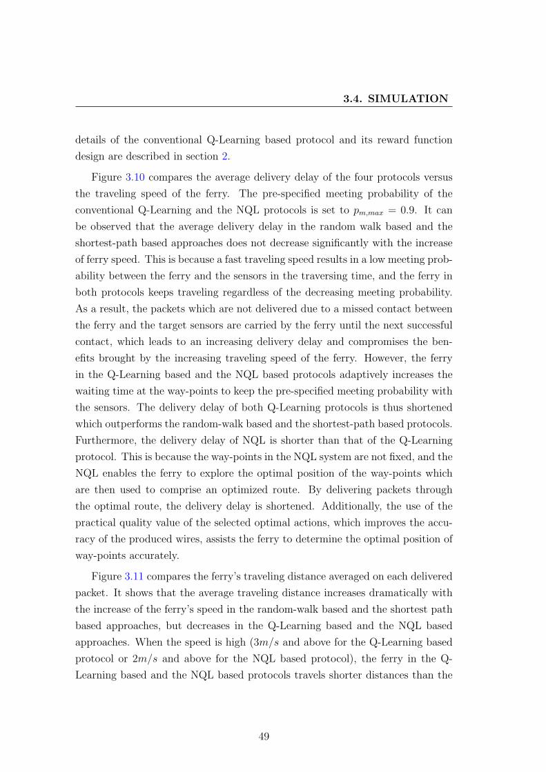
3.4. SIMULATION
details of the conventional Q-Learning based protocol and its reward function
design are described in section 2.
Figure 3.10 compares the average delivery delay of the four protocols versus
the traveling speed of the ferry. The pre-specified meeting probability of the
conventional Q-Learning and the NQL protocols is set to pm,max = 0.9. It can
be observed that the average delivery delay in the random walk based and the
shortest-path based approaches does not decrease significantly with the increase
of ferry speed. This is because a fast traveling speed results in a low meeting prob-
ability between the ferry and the sensors in the traversing time, and the ferry in
both protocols keeps traveling regardless of the decreasing meeting probability.
As a result, the packets which are not delivered due to a missed contact between
the ferry and the target sensors are carried by the ferry until the next successful
contact, which leads to an increasing delivery delay and compromises the ben-
efits brought by the increasing traveling speed of the ferry. However, the ferry
in the Q-Learning based and the NQL based protocols adaptively increases the
waiting time at the way-points to keep the pre-specified meeting probability with
the sensors. The delivery delay of both Q-Learning protocols is thus shortened
which outperforms the random-walk based and the shortest-path based protocols.
Furthermore, the delivery delay of NQL is shorter than that of the Q-Learning
protocol. This is because the way-points in the NQL system are not fixed, and the
NQL enables the ferry to explore the optimal position of the way-points which
are then used to comprise an optimized route. By delivering packets through
the optimal route, the delivery delay is shortened. Additionally, the use of the
practical quality value of the selected optimal actions, which improves the accu-
racy of the produced wires, assists the ferry to determine the optimal position of
way-points accurately.
Figure 3.11 compares the ferry’s traveling distance averaged on each delivered
packet. It shows that the average traveling distance increases dramatically with
the increase of the ferry’s speed in the random-walk based and the shortest path
based approaches, but decreases in the Q-Learning based and the NQL based
approaches. When the speed is high (3m/s and above for the Q-Learning based
protocol or 2m/s and above for the NQL based protocol), the ferry in the Q-
Learning based and the NQL based protocols travels shorter distances than the
49

3. A NEURAL-Q-LEARNING BASED APPROACH FOR DELAYTOLERANT UNDERWATER WIRELESS SENSOR NETWORKS
shortest-path based protocol to deliver a packet. Compared with the Q-Learning
based protocol, the average traveling distance of the ferry in the NQL protocol
is shorter. This is consistent with the results shown in Figure 3.10.
In Figure 3.12 where the traveling speed of the ferry is set to 4.5m/s, we
compare the average delivery delay of the protocols at various values of pm,max.
It can be observed that the delivery delay of the random-walk based and the
shortest-path based approaches remains stable. On the other hand, the delivery
delay of the Q-Learning based and the NQL based protocols keeps decreasing with
the increase of pm,max. This is because the waiting time is fixed to zero for the
random-walk based and the shortest path based approaches, but varies inversely
with the ferry’s speed for the Q-Learning based and the NQL based approaches.
Moreover, the NQL achieves a much shorter delivery delay than the conventional
Q-Learning based protocol. Figure 3.13 compares the ferry’s traveling distance
averaged on each delivered packet, which is consistent with the results shown in
Figure 3.12.
3.5 Conclusion
One main focus of current researches on delay tolerant networks is to increase
the meeting probabilities of sensors, which are important for achieving a good
throughput, lowering the delivery cost and keeping a short delivery delay. In
underwater acoustic wireless sensor networks (UA-WSNs), this problem becomes
challenging due to the unique properties of underwater environments.
In this chapter, we proposed a Neural-Q-Learning (NQL) based delay tolerant
protocol for UA-WSNs. The proposed protocol enables the ferry to determine
the optimal position of way-points in a two-dimensional continuous space, which
comprise an efficient traveling route to reduce the delivery delay and delivery
cost while maximizing the meeting probabilities between the ferry and sensors.
Through simulations, we have demonstrated the feasibility and efficiency of the
NQL protocol in UA-WSNs.
50

3.5. CONCLUSION
0.5 1 1.5 2 2.5 3 3.5 4 4.5 52000
4000
6000
8000
10000
12000
14000
16000
ferry speed (m/s)
aver
age
deliv
ery
dela
y (s
econ
ds)
Random BasedShortest−path BasedConventional Q−LearningNeural−Q−Learning
Figure 3.10: Delivery delay versus ferry speed
0.5 1 1.5 2 2.5 3 3.5 4 4.5 50
10
20
30
40
50
60
70
80
90
100
ferry speed (m/s)
trave
ling
dist
ance
of f
erry
per
del
iver
ed p
acke
t (m
/pkt
)
Random BasedShortest−path BasedConventional Q−LearningNeural−Q−Learning
Figure 3.11: Ferry’s traveling distance per delivered packet versus ferry speed
51

3. A NEURAL-Q-LEARNING BASED APPROACH FOR DELAYTOLERANT UNDERWATER WIRELESS SENSOR NETWORKS
0.1 0.2 0.3 0.4 0.5 0.6 0.7 0.8 0.9 13000
4000
5000
6000
7000
8000
9000
10000
11000
12000
pre−specific maximum meeting probability pm,max
aver
age
deliv
ery
dela
y (s
econ
ds)
Random BasedShortest−path BasedConventional Q−LearningNeural−Q−Learning
Figure 3.12: Delivery delay versus pm,max
0.1 0.2 0.3 0.4 0.5 0.6 0.7 0.8 0.9 10
20
40
60
80
100
120
140
160
180
pre−specific maximum meeting probability pm,max
trave
ling
dist
ance
of f
erry
per
del
iver
ed p
acke
t (m
/pkt
)
Random BasedShortest−path BasedConventional Q−LearningNeural−Q−Learning
Figure 3.13: Ferry’s traveling distance per delivered packet versus pm,max
52

Chapter 4
Multiple Ferries
Neural-Q-Learning Based
Approach for Delay Tolerant
Underwater Acoustic Wireless
Sensor Networks
4.1 Introduction
In recent decades, many existing protocols and schemes have shown the effec-
tiveness of the Q-Learning algorithms in underwater acoustic wireless commu-
nications. However, most of these approaches are single agent based. Recent
researches [13, 14, 77] have revealed that a robust multi-agent system which en-
ables multiple intelligent agents to jointly solve tasks or to maximize performance
through their interactions is capable of allowing a significant increase in system
efficiency without requiring a proportional increase of consumed resources (e.g.
energy, channel bandwidth, etc.) [48, 74]. As a result, it is necessary to develop
a cooperative multi-agent based intelligent method which can effectively and ef-
ficiently determine the optimal action in a large, or even continuous, action set
at a given system state.
53
4. MULTIPLE FERRIES NEURAL-Q-LEARNING BASEDAPPROACH FOR DELAY TOLERANT UNDERWATERACOUSTIC WIRELESS SENSOR NETWORKS
In this chapter, we propose a cooperative multi-agent Neural-Q-Learning
(MNQL) [26, 39, 71] based delay-tolerant protocol for underwater acoustic wire-
less sensor networks (UA-WSNs). The proposed MNQL protocol reduces the de-
livery delay by enabling each ferry (i.e. the intelligent agent) to find an efficient
and relatively short traveling route which inter-connects the optimized way-points
to deliver data packets between sensors. The optimal position of the way-points
which are dynamic in a two-dimensional continuous space is determined by the
ferries based on their independent learning from environments. Compared with
the conventional Q-Learning algorithms, the MNQL agents avoid searching a large
or infinite lookup table. Additionally, the system performance is improved by de-
ploying multiple intelligent agents (i.e. the ferries) and enabling the cooperations
between them to achieve desirable outcomes. Each ferry in the proposed coop-
erative multi-agent system exercises individual choice while achieving an overall
effect that benefits not only itself but also the whole system. More specifically,
a delay-tolerant underwater acoustic wireless sensor network is modeled as a co-
operative MNQL system, in which the NQL algorithm produces a continuous
q-curve to replace the discrete q-table used in the conventional Q-Learning algo-
rithms, and the joint action learner (JAL) algorithm [17] is employed to establish
a cooperative structure among the ferries to coordinate their actions [47, 93]. In
such multi-agent systems, the inter-agent communication is one of the important
requirements for developing the coordination strategy and intelligence decision.
But in underwater acoustic communications, the reliable real-time node-to-node
communications is impractical due to the communication-deficient environments
(e.g. constrained bandwidth of channel, limited communication range and long
propagation delay). For maintaining the robust efficiency of multi-agent systems,
each intelligent agent in the proposed system incorporates a behavior predictor
and a local database to keep track of the up-to-date behavior of other agents.
In the proposed delay tolerant UA-WSN, the network consists of a number
of mobile ferries and a number of static sensors. The sensors are assumed to
be sparsely-distributed, energy-constrained, stationary, and consequently are not
capable of peer to peer sensor communications. Thus a number of ferries are
employed to travel around the deployment field to collect, carry and deliver data
packets between sensors. A specific position where a ferry contacts with a specific
54

4.2. RELATED WORK
sensor is known as a way-point. The traveling route of each ferry consists of a
number of segments, each of which connects two way-points. The ferries have
the freedom to determine the position and the order of the way-points to be
visited according to their independent learning. The state of the MNQL system
is presented by the collection of the index number of the sensors which are being
visited by the ferries at the given time instant. The action of the system is defined
as an action vector consisting of the actions of all the ferries, each of which is a
specific way-point to be visited by a specific ferry. Simulation results show that
the MNQL system improves the system performance by coordinating the agents
to explore an optimized traveling route for each of the ferries so as to maximize
the meeting probabilities between the ferries and the sensors.
The rest of this chapter is organized as follows. In section 4.2, the multi-
agent system and the joint action learner (JAL) algorithm are briefly reviewed.
The detailed implementations of the proposed cooperative MNQL system are
described in section 4.3. Then, simulation configurations and results are given in
section 4.4. Finally, the conclusion is drawn in section 4.5.
4.2 Related Work
In this chapter, the proposed cooperative multi-agent system with a continuous
action set employs the Neural-Q-Learning [87] approach to determine the optimal
position of way-points in a two-dimensional continuous space. These optimized
way-points lead to an efficient traveling route to reduce the delivery delay and
delivery cost. In this chapter, the joint action learner (JAL) [17] algorithm is
employed to establish the cooperation between ferries. The related works are
briefly reviewed as follows.
Many existing schemes and protocols using the NQL algorithm are single-
agent based systems [9, 21, 27, 51, 84]. For improving the system performance,
it is necessary to extend the algorithm to a cooperative multiple-agent based sys-
tem. In multi-agent reinforcement learning (MARL) systems, there are multiple
intelligent agents deployed in the systems, in which each agent has the freedom
to determine actions according to its independent learning from the environment
[4]. From the perspective of each individual agent, the actions of other agents
55

4. MULTIPLE FERRIES NEURAL-Q-LEARNING BASEDAPPROACH FOR DELAY TOLERANT UNDERWATERACOUSTIC WIRELESS SENSOR NETWORKS
are treated as part of the environment influencing the action determination pro-
cess of the agent. Therefore, the environment is inherently non-stationary since
the other agents are free to change their behaviors as they also learn and adapt
[83]. As a result, the actions of other agents must be taken into the consideration
by each individual agent due to the mutual influence among the agents. Corre-
spondingly, the updating rule of an individual and independent agent in a typical
MARL system is defined as follows,
Q(s,~a) = (1− α)Q(s,~a) + α[r(s, ai) + γV (s′)] (4.1)
where s is the system state, ~a is the action vector consisting of the action of all
the agents, Q(s,~a) is the quality value of the action vector ~a at the state s ,
V (s′) is the state value of the state s′, r(s, ai) is the instant reward that agent i
obtained by taking the action ai at the state s, γ is the discount factor and α is
the learning rate.
In recent decades, a number of approaches have been proposed and imple-
mented for MARL systems (e.g. Independent Learner (IL) [17, 82], Joint Action
Learner (JAL) [17, 82], Distributed Value Function (DVF) [54, 72], etc.). The
proposed approach employs the JAL algorithm, which was first introduced by
Claus and Boutilier [17] as a multi-agent extension to the conventional single
agent Q-Learning algorithms. Each JAL agent maintains an explicit model of
the opponents (i.e. other ferries) at each state to compute the value function
V (s) (i.e. the value of state s). More specifically, the agent i assumes that its
opponents are stationary, i.e. ~a = ai, a−i where ai is agent i’s current action
and a−i is the collection of the most recent actions of the other agents (i.e. all
agents except agent i). The assumed model of the opponent requires the empirical
frequencies of the action taken by an agent. By using this model, the updating
rule of agent i in JAL is as follows [17],
Q(s, ai, a−i) ← (1− α)Q(s, ai, a−i) + α(r(s, ai) + γV (s′)) (4.2)
where
V (s′) = maxai
∑a−i
C(s′, a−i)
n(s′)Q(s′, ai, a−i) (4.3)
56

4.3. SYSTEM DESCRIPTION
and C(s, a−i) = C(s, a−i) + 1.
4.3 System Description
In this section, we describe the proposed cooperative Multi-agent Neural-Q-
Learning (MNQL) algorithm as applied in a distributed delay tolerant UA-WSN
which consists of m static sensors and n mobile ferries. Due to the constrained
battery power, the transmission range of each sensor is very limited. As a re-
sult, the transmission area of any two sensors does not overlap and the sensors
cannot communicate with each other for exchanging information. Moreover, for
the purpose of conserving energy, each sensor periodically transits between two
operational states: the active state (high-power fully functional mode) and the
sleep state (low-power partially functional mode). In the active state, the sensor
is fully functional and is able to transmit and receive, while in the sleep state
the sensor cannot take part in the network activity. Each sensor switches to
the active state according to a Poisson process with a rate λ (in times/second).
Within a unit of time (i.e. one second), the probability that the sensor switches
to the active state for k times is expressed as p(k) = e−λλk/k!. As a result, the
probability of that sensor remaining in the sleep state (i.e. k = 0) in one second is
ps = p(k = 0) = e−λ. In either state, each sensor keeps generating data packets at
random intervals according to a Poisson process with a rate g packets/second and
stores these packets in the local buffer as a first-in-first-out queue with tail-drop.
Note here that the generating rates may be different among sensors.
Compared with the sensors, the ferries are much more powerful in terms of
energy supply, storage space and computational abilities. Thus, we assume that
the storage space of the ferry is infinite. On the other hand, the ferry is equipped
with mobility and is capable of continually traveling around the deployment area
to collect/deliver data packets from/to sensors. The traveling route of the ferry
comprises a set of segments. Each of these segments connects two way-points,
each of which is defined as a specific position where the ferry can communicate
with a certain sensor. Obviously, a way-point must be within the transmission
range of at least one sensor. Since there is no intersection between the transmis-
sion areas of any two sensors, each sensor, e.g. sensor i, must have a unique and
57

4. MULTIPLE FERRIES NEURAL-Q-LEARNING BASEDAPPROACH FOR DELAY TOLERANT UNDERWATERACOUSTIC WIRELESS SENSOR NETWORKS
dedicated way point denoted by wi. The host sensor of wi is denoted by h(wi).
Given a way-point vector ~w = w1, w2, · · ·, h(~w) = h(w1), h(w2), · · · denotes
the collection of the host sensors of the way-points in the vector. Note here that
the positions of way-points are dynamic within the transmission range of their
host sensors and are determined by the ferry. We also assume that the speed and
direction of the ferry does not change when traveling between any two way-points
(i.e. the ferry travels along a straight line between two way-points at a constant
speed). When traveling into the transmission range of a target sensor (the host
sensor of a specific way-point), the ferry broadcasts beacon packets at a constant
rate to detect the presence of its target sensor in the surrounding area. All the
sensors keep listening to the underwater channel. If the beacon packet is received
by the desired sensor, an acknowledgement packet is generated by the sensor and
sent to the ferry immediately. After receiving the acknowledgement packet, the
ferry looks up its local buffer and transmits (uploads) the data packets targeting
to this sensor and collects (downloads) all the data packets from this sensor’s lo-
cal buffer. The upload and download process is known as a service. The traveling
speed of the ferry (0.5 ∼ 10m/s [7]) is much slower than the propagation speed of
acoustic wave in the underwater environment (1500m/s [85]), thus it is assumed
that the ferry doesn’t stop its travel during services. In the proposed approach,
each ferry is modeled as an individual and independent intelligent agent which
determines not only the optimal visiting targets, but also the optimal position of
way-points, based on its independent learning from the environment. Figure 4.1
shows the flow chart of the MNQL algorithm.
4.3.1 The Cooperative Multi-agent Neural-Q-Learning Frame-
work
4.3.1.1 System State Space
In the proposed system, the whole network is considered as a multiple agent
Neural-Q-Learning system, in which each ferry acts as an individual and inde-
pendent agent. The system states are discrete and related to the sensors that the
ferries visit. For instance, when the kth ferry is visiting and servicing sensor i at
time t, the state of ferry k is defined as sk = i. The state of all the ferries comprise
58
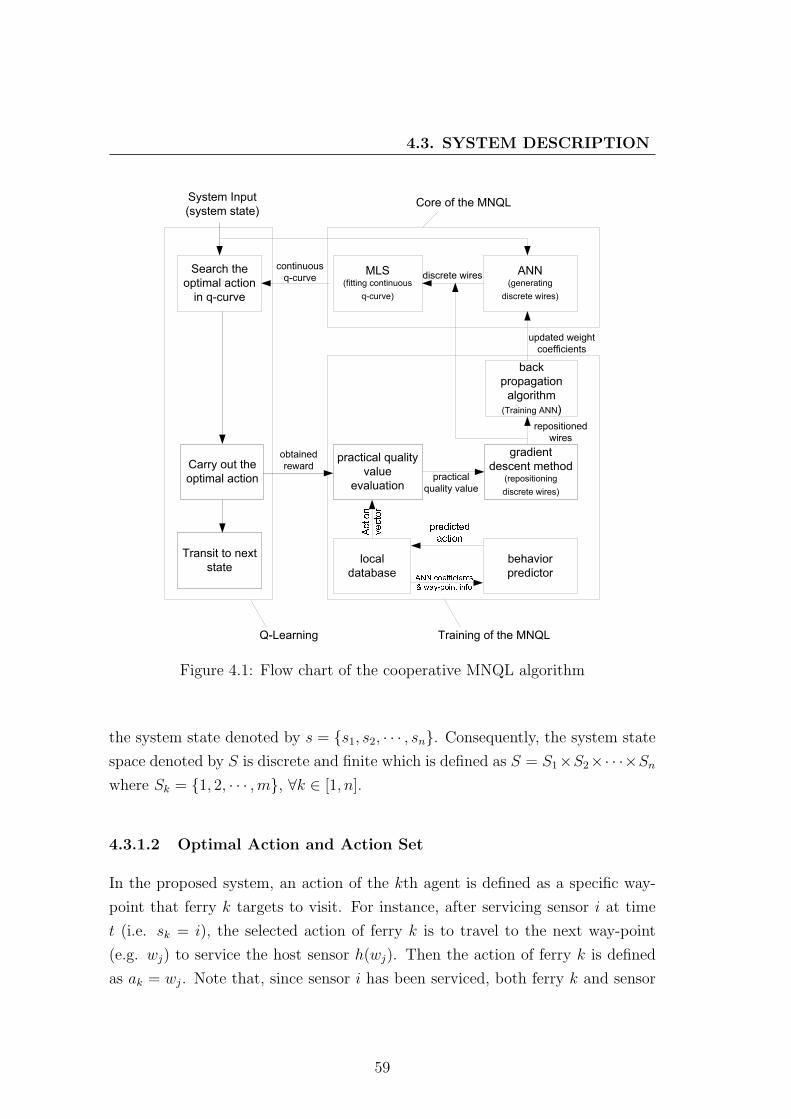
4.3. SYSTEM DESCRIPTION
Search the optimal action
in q-curve
Transit to next state
Carry out the optimal action
practical qualityvalue
evaluation
gradient descent method
(repositioning discrete wires)
MLS(fitting continuous
q-curve)
ANN(generating
discrete wires)
back propagation
algorithm(Training ANN)
System Input(system state)
obtained reward
practical quality value
discrete wirescontinuous
q-curve
Training of the MNQL
Core of the MNQL
Q-Learning
repositionedwires
updated weight coefficients
! "
Figure 4.1: Flow chart of the cooperative MNQL algorithm
the system state denoted by s = s1, s2, · · · , sn. Consequently, the system state
space denoted by S is discrete and finite which is defined as S = S1×S2×· · ·×Sn
where Sk = 1, 2, · · · ,m, ∀k ∈ [1, n].
4.3.1.2 Optimal Action and Action Set
In the proposed system, an action of the kth agent is defined as a specific way-
point that ferry k targets to visit. For instance, after servicing sensor i at time
t (i.e. sk = i), the selected action of ferry k is to travel to the next way-point
(e.g. wj) to service the host sensor h(wj). Then the action of ferry k is defined
as ak = wj. Note that, since sensor i has been serviced, both ferry k and sensor
59

4. MULTIPLE FERRIES NEURAL-Q-LEARNING BASEDAPPROACH FOR DELAY TOLERANT UNDERWATERACOUSTIC WIRELESS SENSOR NETWORKS
i do not have buffered packet to exchange. As a result, sensor i is excluded from
the set of sensors to be serviced by ferry k, i.e. i /∈ i− where i− denotes the set of
host sensors that ferry k may visit (i.e. i− = 1, · · · , i−1, i+1, · · ·m). Thus the
action set of ferry k at time t is defined as Ak =⋃
x∈i−Rx. In other words, the action
set of ferry k is the union of the transmission area of all sensors except sensor i.
The next way-point must be wj ∈⋃
x∈i−Rx, where Rx is the transmission area of
sensor x. Furthermore, by using polar coordinates, the position of a way-point wi
relative to its host sensor (e.g. sensor i ) can be represented by (θwi, rwi
)i where
θwiand rwi
are the angle and distance of the way-point wi relative to the position
of its host sensor i. In other words, an action a of ferry k is interpreted as the
polar coordinates of the way-point wi, i.e. ak = (θwi, rwi
)i, where θwi∈ [0, 2π],
rwi∈ [0, r] and r is the maximum transmission range of the sensor.
Differing from the single agent reinforcement learning systems, the action
of the proposed multi-agent system is an action vector ~a consisting of the ac-
tion of all the agents at the given state, i.e. ~a = a1, a2, · · · where ak de-
notes the action of agent k. Each single agent aims at determining the opti-
mal position of the way-point that it targets to visit, which achieves the max-
imum quality value at the current state. At a given system state, e.g. s =
s1, s2, · · · , sn in which sk = i, the highest quality value that ferry k can achieve
is q∗k = maxj∈i−
q∗(j) = maxq∗(1), · · · , q∗(i − 1), q∗(i + 1), · · · , q∗(m) where q∗(j)
denotes the quality value Q(s, a∗k(j), a−k), a−k = a1, · · · , ak−1, ak+1, · · · , anand a∗k(j) = arg max
ak∈Rj
Q(s, ak, a−k). Note here that, when evaluating the qual-
ity value, an agent assumes the actions of other agents remain stationary, i.e.
a−k, which is the action vector consisting of the most recent actions of all the
ferries except ferry k, remains unchanged. Correspondingly, ferry k’s optimal
action (i.e. the optimal position of the way-point of the target sensor x) is
a∗k = a∗k(x) = arg maxak∈Rx
Q(s, ak, a−k) where x is the index number of the tar-
get sensor selected by ferry k and x = arg maxj∈i−
q∗(j).
In the example shown in Figure 4.2, two ferries and four sensors are deployed
in the field. The system state at time t is st = i, j2 since the ferry 1 and ferry 2
are visiting the way-points wi and wj2 corresponding to their host sensors i and
j2. The action set is At = A1 ×A2 where A1 = j1, j2, j3 and A2 = i, j1, j3. If
60

4.3. SYSTEM DESCRIPTION
Figure 4.2: System state and action set
ferry 1 and ferry 2 determine wj1 and wj3 as their optimal actions at the current
state, respectively, the system action is ~a∗t = a1, a2 where a1 = (θwj1, rwj1
)j1
and a2 = (θwj3, rwj3
)j3 . By carrying out the selected action ~a∗t , the system state
transits to st′ = j1, j3.
4.3.2 Generating the Q-Curve
Differing from the conventional Q-Learning algorithms, the proposed MNQL sys-
tem approximates the optimal action by searching the greatest value(s) of a con-
tinuous q-curve which is produced by an ANN along with a wire-fitting interpo-
lator. The ANN is used to generate a fixed number of discrete samples (known as
control wires) which are then used in the wire-fitting interpolator to fit a contin-
uous q-curve. The implementation details of these two techniques are depicted
in section 3.3.2.
61

4. MULTIPLE FERRIES NEURAL-Q-LEARNING BASEDAPPROACH FOR DELAY TOLERANT UNDERWATERACOUSTIC WIRELESS SENSOR NETWORKS
4.3.3 Improvement of the ANN and the Q-Curve
The selection of the optimal way-points relies on the q-curve. Thus it is necessary
to keep improving the accuracy of the curve. In this section, we depict the details
of the training of the ANN and the adjustments of the q-curve by using a practical
quality value.
4.3.3.1 Evaluation of the Practical Quality Value
Once an optimal action a∗k (i.e. the optimal position of a way-point) is determined
and carried out by the agent k at state s, ferry k moves to the selected way-point
and the system transits to a new state s′. By taking this action, the agent k
derives the instant reward/penalty r(s, a∗k) from the environment accordingly.
The reward function employed by the proposed system is the same as the one
given in section 3.3.3.1. Based on these parameters, a practical quality value
denoted by Q(s, a∗k, a−k) is evaluated using (4.2).
In the proposed system, each single ferry’s action could influence the decision
and performance of other ferries. For instance, after being serviced by a ferry,
the sensor’s buffer queue is emptied. If another ferry visits this sensor at this
moment, no data packets can be collected from the sensor, which degrades the
performance of that ferry. Although the sensor which was just serviced recently
cannot be ruled out from the action set of other ferries, its servicing priority
is much lower than those who have relatively more data packets waiting in the
buffer queue. Due to the mutual influence among the ferries, the cooperation
between them becomes important for the entire system to keep a high efficiency.
Differing from the conventional JAL where the value of the next state (i.e. V (s′)
in equation (4.2)) is estimated before the action is executed, the value of the
new state in the proposed cooperative MNQL is a real-time state value which
is derived by the agent after reaching the new state s′. More specifically, after
a ferry arriving at the selected way-point, the system state transits to s′. The
greatest value(s) of the q-curve corresponding to the system state s′ is used as
the state value V (s′). Consequently, the agents in the proposed system do not
need to maintain the explicit models of the opponent(s) at each state which are
used to calculate the estimated state value in the conventional JAL approaches.
62

4.3. SYSTEM DESCRIPTION
When evaluating a practical quality value, an individual agent must consider
other agents’ states and actions. When ferry k carries out the action ak = wj at
a given system state s = s1, s2, · · · , sn in which ferry k’s state is sk = i, the
system transits to a new state s′ = s′1, s′2, · · · , s′n. Let ~ak = ak, a−k, then ferry
k evaluates the quality value of the action taken at the state s as follows.
Q(s,~ak) = (1− α)Q(s, ~α) + α(r(s, ak) + γV (s′)) (4.4)
where ~α is an action vector consisting of the most recent actions of all the ferries
which satisfies H(~α) = H(~ak) and H(·) denotes the collection of the host sensors
of the actions in the vector (·).
4.3.3.2 Agent Behavior Prediction
In the evaluation of the practical quality value of the selected action at the given
state, each agent must know the exact action vector consisting of the action
of all other ferries. But it is difficult (or costly) to derive such information in
the proposed system due to the failure potentialities and limited communication
features (such as bandwidth limitations, limited ranges, or unexpected delays)
of underwater communication channels. As a result, it is important for each
ferry to be able to predict the actions/behaviors of other ferries which are out
of the communication range (i.e. when data synchronization between ferries is
difficult/imposssible). In the proposed system, a behavior predictor is employed
to estimate the actions of other agents according to the action/state data stored
in a local database [78].
Each ferry maintains a database storing the up-to-date action/state informa-
tion of other ferries [14, 77]. Each record of the database corresponds to a specific
ferry and consists of the set of weighting coefficients of ANN of that ferry, the
state/action details (including the coordinates of the selected way-point and index
number of both the previous serviced sensor and the next target sensor of that
ferry) and the time of the most recent update. When traveling in the deployment
field, each ferry (e.g. ferry k) keeps broadcasting beacon packets consisting of
the up-to-date action/state details of itself. These information is used to update
the record pertaining to ferry k in the database of those ferries which receive the
63

4. MULTIPLE FERRIES NEURAL-Q-LEARNING BASEDAPPROACH FOR DELAY TOLERANT UNDERWATERACOUSTIC WIRELESS SENSOR NETWORKS
beacon messages.
A behavior predictor consists of an ANN and a moving least square interpo-
lator, both of which have the structure as described in section 3.3.2. Moreover,
in the proposed system, all the ferries are assumed to be homogeneous, i.e. they
employ the identical ANN structure (e.g. the number of layers, the number of
neurons in each layer, and the activation functions) and wire-fitting interpola-
tor algorithm. Note here that the weighting coefficients of connections between
neurons which depend on the adjustments of individual agents’s training process
may be different. When the action and state of another ferry (e.g. ferry j) is
required, ferry k looks up its local database to check the corresponding record
of ferry j. If the record is valid, i.e. the time length since the last update of
the record is less than a pre-specified maximum active duration, the action and
state data of ferry j stored in the database can be used in the evaluation directly.
Otherwise the database record is outdated, in which case the behavior predictor
of ferry k generates an ANN with the weighting coefficients of ferry j, and feeds
in the coordinates of the selected way-point of ferry j’s target sensor as the input
parameters to predict a plausible action of ferry j. The predicted action is then
used as the up-to-date information of ferry j to update the corresponding record
in ferry k’s local database. Once the up-to-date action/state data of all the ferries
is derived, the evaluation of the practical quality value is carried out by ferry k.
In the evaluation of the practical quality value, the reward function plays an
important role as it determines the behavior of the intelligent agent in the long
term. For our proposed approach, the main considerations in the design of the
reward function include the ferry’s traveling distance, the ferry’s waiting time at
a way-point, the effective bandwidth, the target sensor’s queue length and the
contact between the ferry and the target sensor, which are depicted in section
3.3.3.1. In the proposed MNQL system, the practical quality value evaluated
based on the real-time reward and real-time value of the next state represents
the actual quality of the selected action ak at the state s, which deserves a higher
accuracy than the estimated quality values of the conventional JAL algorithms.
After an optimal action a∗k is carried out by the ferry k at a given state
s, the ferry k evaluates the practical quality value Q(s, a∗k, ak−) which is then
converted into a ζ∗q factor by ζ∗q = (Q(s,a∗k,ak−)−qinit
C+1)/2. The reposition of wires
64

4.4. SIMULATION
with the gradient-descent method and the training of ANN with back propagation
are described in section 3.3.3.2 and 3.3.3.3.
4.4 Simulation
In this section, we apply the proposed cooperative Multi-agent Neural-Q-Learning
(MNQL) based protocol to various network topologies and use simulation results
to demonstrate the effectiveness and efficiency of the proposed protocol. More
details are given as follows.
4.4.1 Configurations
We consider a randomly generated network consisting of 20 sensors (i.e. m = 20)
uniformly and sparsely deployed over a 2000m× 2000m square area. The maxi-
mum transmission range of the sensors is 50 meters. Each sensor independently
generates data packets according to a Poisson process with rate g packets/second
where g ∈ [0.01, 0.05]. Note that the generating rates may be different between
sensors. The size of each generated data packet is 100kB (i.e. 100× 1024 bytes).
The maximum size of buffer queue is 500 packets for all the sensors. The traveling
speed of the ferry, denoted by v, varies from 1m/s to 10m/s in 1m/s increments.
The sleep/active switching rate is set to λ times/second where λ ∈ [0.005, 0.07].
In the MNQL implementation, the discount factor γ = 0.5, the learning rate
αt = 1/t, t = 1, 2, · · ·, the number of wires and the number of neurons in the
hidden layer of ANN are set to 10 and 20, respectively. The ferries in MNQL
are capable of determining the optimal position of the way-points within their
host sensor’s transmission range which is a two-dimensional continuous space.
Considering the size of the deployment field and the number of employed AUVs,
the probability of crash is small in the proposed system [88]. For the purpose
of eliminating potential crashes between the ferries, each ferry is programmed to
travel at a constant and dedicated depth above the deployment field. The max-
imum active duration of database records is pre-specified as dmax
vwhere dmax is
the maximum distance between any two sensors. The maximum effective band-
width Bmax of an underwater acoustic communication channel is set to 100kHz.
65

4. MULTIPLE FERRIES NEURAL-Q-LEARNING BASEDAPPROACH FOR DELAY TOLERANT UNDERWATERACOUSTIC WIRELESS SENSOR NETWORKS
The simulation results are shown in section 4.4.2. Each simulation runs 5 × 10⁵
seconds. Each data point is the average of twenty independent simulations.
4.4.2 Simulation Results
4.4.2.1 Performance of the MNQL Protocol
In this section, the performance of the proposed MNQL protocol is evaluated in
various scenarios. The maximum waiting time in the MNQL protocol is deter-
mined by the ferries as described in section 3.3.3.1. The number of ferries is set to
2,3 and 5, respectively (i.e. n = 2, 3, 5). In Figure 4.3 where the traveling speed of
the ferries is fixed at 10m/s, the total number of delivered packets increases when
the pre-specified max meeting probability pm,max increases from 0.1 to 1 with 0.1
increments. This is because a low pm,max leads to a short maximum waiting time
and consequently a low meeting probability between the ferries and the sensors,
which increases the number of packets that cannot be delivered due to the missed
contacts between the ferries and the sensors. These packets have to be carried by
the ferries until the next successful contacts with the sensors, which result in not
only a low number of delivered packets but also a significantly long delivery delay
and a long average traveling distance of the ferries, as shown in Figure 4.4 and
Figure 4.5. It can also be observed that, when there are more ferries deployed,
the total number of delivered packets increases. This is reasonable since more
ferries lead to a higher frequency of the sensors being visited which consequently
result in more collected and delivered packets. For the same reason, the average
delivery delay and the average traveling distance of the ferries decrease, as shown
in Figure 4.4 and Figure 4.5.
Figure 4.6 shows that the total number of delivered packets increases with the
increase of the traveling speed of the ferries since a faster speed of the ferries not
only increases the frequency of the sensors being visited but also accelerates the
learning process of the MNQL agents. Figure 4.7 shows that the average delivery
delay decreases with the increase of the traveling speed of the ferries since a faster
traveling speed of the ferry leads to a shorter traveling time which consequently
shortens the delivery delay. In Figure 4.8, when the speed increases, the ferries’
traveling distance averaged on each delivered packet decreases dramatically and
66

4.4. SIMULATION
0.1 0.2 0.3 0.4 0.5 0.6 0.7 0.8 0.9 10.4
0.6
0.8
1
1.2
1.4
1.6
1.8
2x 10⁴
pre−specific maximum meeting probability pm,max
tota
l num
ber o
f del
iver
ed p
acke
ts
2 ferries3 ferries5 ferries
Figure 4.3: total delivered packets versus pm,max
0.1 0.2 0.3 0.4 0.5 0.6 0.7 0.8 0.9 11000
2000
3000
4000
5000
6000
7000
8000
pre−specific maximum meeting probability pm,max
aver
age
deliv
ery
dela
y (s
econ
ds)
2 ferries3 ferries5 ferries
Figure 4.4: delivery delay versus pm,max
67

4. MULTIPLE FERRIES NEURAL-Q-LEARNING BASEDAPPROACH FOR DELAY TOLERANT UNDERWATERACOUSTIC WIRELESS SENSOR NETWORKS
0.1 0.2 0.3 0.4 0.5 0.6 0.7 0.8 0.9 120
30
40
50
60
70
80
90
100
110
120
pre−specific maximum meeting probability pm,max
trave
ling
dist
ance
of f
erry
per
del
iver
ed p
acke
t (m
/pkt
)
2 ferries3 ferries5 ferries
Figure 4.5: Ferry’s traveling distance per delivered packet versus pm,max
1 2 3 4 5 6 7 8 9 100
0.2
0.4
0.6
0.8
1
1.2
1.4
1.6
1.8
2x 10⁴
ferry speed (m/s)
tota
l num
ber o
f del
iver
ed p
acke
ts
2 ferries3 ferries5 ferries
Figure 4.6: total delivered packets versus speed
68

4.4. SIMULATION
converges to a steady-state value quickly. Additionally, deploying more ferries
is capable of increasing the number of delivered packets and lowering both the
delivery delay and the ferries’ average traveling distance.
4.4.2.2 Performance Comparison with Existing Protocols
In this section, we compare the performance of the proposed MNQL protocol with
other existing protocols which include the random-walk (RW) [73] based, shortest-
path (SP) [92] based, the conventional Q-Learning (QL) algorithm [95] based and
the Neural-Q-Learning (NQL) [96] based protocols. The number of employed
ferries is set to 5 in all these protocols. Note that the multiple ferries in the four
benchmarks do not have cooperative relationship between each other, i.e. each
ferry determines the next visiting target individually and independently without
considering other ferries. The position of way-points are fixed at the position of
their host sensors in the RW, SP and QL protocols, but are dynamic within the
transmission range of their host sensors in the NQL and MNQL approaches. In
the shortest path based approach, the ferry determines a shortest traveling path
according to the deployment of all static sensors before servicing any sensors and
follows the pre-specified shortest route to visit and service the sensors. Once
determined, the route remains unchanged until the end of a mission. Whereas,
the fixed route does not exist in the random-walk based approach used by the
data mules protocol since the ferry randomly determines the next target (i.e.
the sensor which the ferry is going to service/visit) after visiting a sensor. The
maximum waiting time in both RW and SP protocols is set to zero, i.e. the ferry
doesn’t wait at way-points when the response is not heard from the targeting
sensor. In the QL, NQL and MNQL protocols, the maximum waiting time is
determined by the ferries as described in section 3.3.3.1. More implementation
details of the conventional Q-Learning based protocol and its reward function
design are described in chapter 2. The details of the NQL protocol is depicted in
chapter 3
In Figure 4.9 where the traveling speed of the ferries is set to 10m/s, we com-
pare the number of total delivered packets of all five protocols at various values of
the pre-specified maximum meeting probability pm,max. It can be observed that,
with the increases of pm,max from 0.1 to 1.0 with 0.1 increments, the number of
69

4. MULTIPLE FERRIES NEURAL-Q-LEARNING BASEDAPPROACH FOR DELAY TOLERANT UNDERWATERACOUSTIC WIRELESS SENSOR NETWORKS
1 2 3 4 5 6 7 8 9 101000
2000
3000
4000
5000
6000
7000
8000
9000
10000
11000
ferry speed (m/s)
aver
age
deliv
ery
dela
y (s
econ
ds)
2 ferries3 ferries5 ferries
Figure 4.7: delivery delay versus speed
1 2 3 4 5 6 7 8 9 1010
20
30
40
50
60
70
80
ferry speed (m/s)
trave
ling
dist
ance
of f
erry
per
del
iver
ed p
acke
t (m
/pkt
)
2 ferries3 ferries5 ferries
Figure 4.8: Ferry’s traveling distance per delivered packet versus speed
70

4.4. SIMULATION
delivered packets significantly increases in the MNQL protocol, but just slightly
increases in the Q-Learning and Neural-Q-Leaning approaches. This is because
the MNQL protocol improves the system efficiency by coordinating the action
of the ferries to avoid servicing a sensor with multiple ferries, which cannot be
achieved by the QL and NQL protocols due to the lack of the cooperative frame-
work among the ferries. In the random-walk based and the shortest-path based
approaches, the total delivered packets remains stable since the ferries in both
protocols keep traveling regardless of the varying meeting probabilities.
It can be observed in Figure 4.10 that the average delivery delay of the
random-walk based and the shortest-path based approaches remains stable, while
the delivery delay of the QL, NQL and MNQL based protocols keeps decreasing
with the increase of pm,max. This is because the waiting time is fixed to zero
for the random-walk based and the shortest path based approaches, but varies
inversely with the ferries’ speed for the QL, NQL and MNQL based approaches.
Moreover, the MNQL achieves a much shorter delivery delay than the QL and
NQL based protocols. Figure 4.11 compares the ferries’ traveling distance av-
eraged on each delivered packet, which is consistent with the results shown in
Figure 4.10.
In Figure 4.12 where the pre-specified maximum meeting probability pm,max
is set to 0.9, the total number of delivered packets in all five protocols increases
with the increase of the traveling speed of the ferries since a faster traveling
speed leads to a shorter traveling time which consequently increases the delivered
packets. The ferries in MNQL deliver less packets than those in the QL and
NQL protocols before the speed reaches 3m/s. After this point, the total number
of the delivered packets in MNQL is greater than that in the QL and NQL
protocols. This is because a slow traveling speed leads to a long traveling period
which causes the expiration of a relatively large number of records in the local
database of MNQL agents. When the practical quality values are evaluated, the
agents have to estimate the action and state for those expired records with the
behavior predictor, which increases not only the online calculation load but also
the probability of errors. The practical quality values evaluated based on the
inaccurately estimated actions result in more errors in the wire repositioning and
ANN training which produce inaccurate q-curves. As a result, the total number
71

4. MULTIPLE FERRIES NEURAL-Q-LEARNING BASEDAPPROACH FOR DELAY TOLERANT UNDERWATERACOUSTIC WIRELESS SENSOR NETWORKS
0.1 0.2 0.3 0.4 0.5 0.6 0.7 0.8 0.9 10.4
0.6
0.8
1
1.2
1.4
1.6
1.8
2x 10⁴
pre−specific maximum meeting probability pm,max
tota
l num
ber o
f del
iver
ed p
acke
ts
RWSPQLNQLMNQL
Figure 4.9: total delivered packets versus pm,max
0.1 0.2 0.3 0.4 0.5 0.6 0.7 0.8 0.9 10
2000
4000
6000
8000
10000
12000
14000
pre−specific maximum meeting probability pm,max
aver
age
deliv
ery
dela
y (s
econ
ds)
RWSPQLNQLMNQL
Figure 4.10: delivery delay versus pm,max
72

4.4. SIMULATION
of the delivered packets of MNQL at a slow traveling speed is less than that of the
QL and NQL protocols. But, a faster speed of the ferries increases the number
of data update communications between ferries which will reduce the number
of expired records and the errors caused by the behavior predictor, and thereby
improve the accuracy of the evaluated practical quality values and the produced q-
curves. Furthermore, a faster speed of the ferries causes faster transitions between
system states which leads to significant dynamic of the system. Since the agents in
the benchmark protocols assume the environment to be stationary, the dynamic
system greatly degrades their performance. The simulation results show that the
ferries in the MNQL protocol quickly adapt to the dynamic environment and
outperforms other approaches when the traveling speed is high (i.e. > 5m/s as
shown in Figure 4.12).
Figure 4.13 compares the average delivery delay of the five protocols versus the
traveling speed of the ferries. It can be observed that the average delivery delay
in all approaches decrease with the increase of the traveling speed of the ferries.
This is reasonable since a faster traveling speed of the ferries leads to a shorter
traveling time which consequently shortens the delivery delay. The ferries in the
QL, NQL and MNQL based protocols decrease the delivery delay by adaptively
increasing the waiting time at the way-points to keep the pre-specified meeting
probability with the sensors. And the delivery delay of MNQL is significantly
shorter than that of the QL and NQL protocols since the coordinations among
the ferries adapt the system to the dynamic environment.
Figure 4.14 compares the ferries’ traveling distance averaged on each delivered
packet. It shows that the average traveling distance increases dramatically with
the increase of the traveling speed in all approaches except the MNQL protocol
where the average traveling distance converges to a steady-state value quickly.
This is because, when there are multiple agents deployed in the system, the
environment is inherently non-stationary from the perspective of each individual
agent. The agents in the QL and NQL protocols fail to determine an optimal
position of way-points due to the frequent transitions of system states caused by
the fast traveling speed of the ferries. But the agents in MNQL are capable of
improving its performance by coordinating their actions. As a result, the average
traveling distance of the ferries in MNQL decreases and quickly converges in such
73
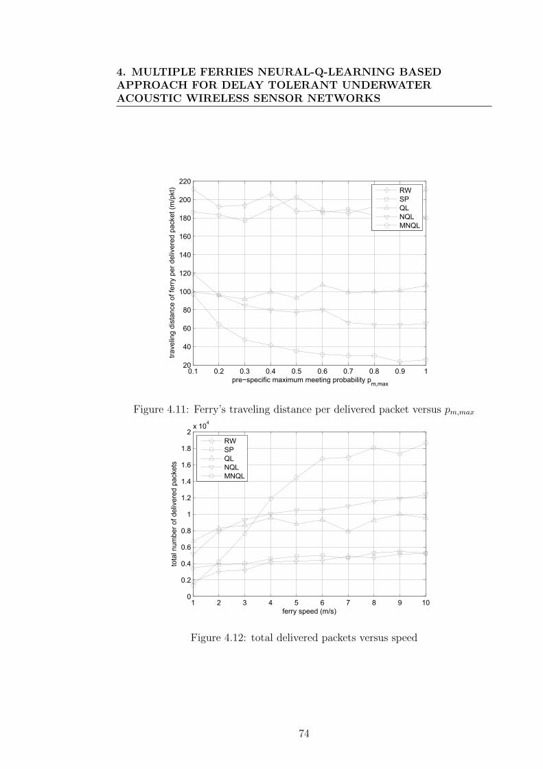
4. MULTIPLE FERRIES NEURAL-Q-LEARNING BASEDAPPROACH FOR DELAY TOLERANT UNDERWATERACOUSTIC WIRELESS SENSOR NETWORKS
0.1 0.2 0.3 0.4 0.5 0.6 0.7 0.8 0.9 120
40
60
80
100
120
140
160
180
200
220
pre−specific maximum meeting probability pm,max
trave
ling
dist
ance
of f
erry
per
del
iver
ed p
acke
t (m
/pkt
)
RWSPQLNQLMNQL
Figure 4.11: Ferry’s traveling distance per delivered packet versus pm,max
1 2 3 4 5 6 7 8 9 100
0.2
0.4
0.6
0.8
1
1.2
1.4
1.6
1.8
2x 10⁴
ferry speed (m/s)
tota
l num
ber o
f del
iver
ed p
acke
ts
RWSPQLNQLMNQL
Figure 4.12: total delivered packets versus speed
74
4.5. CONCLUSION
environment.
4.5 Conclusion
This chapter has proposed a cooperative Multi-agent Neural-Q-Learning (MNQL)
based delay tolerant protocol for UA-WSNs. The proposed protocol enables each
ferry to determine the optimal position of way-points in a two-dimensional contin-
uous space, which comprise an efficient traveling route to reduce the delivery delay
and delivery cost while maximizing the meeting probabilities between the ferries
and sensors. The proposed system achieves a robust performance by employing
the Joint Action Learner algorithm to coordinate the actions of the multiple fer-
ries. Through simulations, we have demonstrated the feasibility and efficiency of
the NQL protocol in UA-WSNs.
75

4. MULTIPLE FERRIES NEURAL-Q-LEARNING BASEDAPPROACH FOR DELAY TOLERANT UNDERWATERACOUSTIC WIRELESS SENSOR NETWORKS
1 2 3 4 5 6 7 8 9 100
0.2
0.4
0.6
0.8
1
1.2
1.4
1.6
1.8
2x 10⁴
ferry speed (m/s)
aver
age
deliv
ery
dela
y (s
econ
ds)
RWSPQLNQLMNQL
Figure 4.13: delivery delay versus speed
1 2 3 4 5 6 7 8 9 100
20
40
60
80
100
120
140
160
180
200
ferry speed (m/s)
trave
ling
dist
ance
of f
erry
per
del
iver
ed p
acke
t (m
/pkt
)
RWSPQLNQLMNQL
Figure 4.14: Ferry’s traveling distance per delivered packet versus speed
76

Chapter 5
Conclusions and Future Work
5.1 Conclusions
In this dissertation, a family of reinforcement learning algorithm based delay tol-
erant protocols designed for fully-distributed underwater acoustic wireless sensor
networks (UA-WSNs) are presented. The proposed protocols explicitly employ
the unique features of underwater acoustic communication channels in their re-
ward function designs to assist each ferry node to determine the optimal visiting
targets and the optimal position of way-points. Some important issues of the
proposed self-adaptive protocols, e.g. the design of reward function, the selection
of the pre-specified maximum meeting probability, the impact of various traveling
speed of the ferries etc., have been presented and analyzed in detail.
The delay-tolerant system developed in chapter 2 models an underwater acous-
tic wireless sensor networks (UA-WSNs) as a single agent reinforcement learning
system in which the position of way-points are fixed at the position of their host
sensors. The ferry is assigned to be the system agent which has the freedom to
select the way-point to be visited. The protocol reduces the delivery delay and
delivery cost by including three factors, namely, the traveling distance factor, the
waiting time factor and the queue length factor, in the reward function design.
The introduced factors enable the ferry to adaptively prolong the waiting time
at way-points to increase the meeting probabilities with sensors. By using the
proposed protocol, the ferry node is capable of learning from the environment
and then adaptively adjusting the relevant parameters of the networks.
77

5. CONCLUSIONS AND FUTURE WORK
The system performance is improved by the protocol presented in chapter 3.
In the proposed system, the ferry has the freedom to determine not only the
order of the way-points it visits, but also their positions which are enabled to be
dynamic within the transmission range of their host sensors. The conventional
reinforcement learning algorithms are not capable of handling such a situation
since the action set of the system is continuous which leads to an infinite look-
up table. As a result, we employ the artificial neural network (ANN) based
Neural-Q-Learning algorithm (NQL) in the system. The ferry in the NQL sys-
tem determines its actions by producing a continuous q-curve, which describes
the relationship between system action and the corresponding quality value at
a given system state, to replace the lookup table used in the conventional Q-
Learning algorithms. Once an optimal action is determined and carried out, the
ferry evaluates a practical quality value which is used not only by the wire-fitting
interpolator to re-generate the q-curve, but also to train the ANN to improve the
accuracy of the produced q-curves. The results show that the use of the arti-
ficial neural network based reinforcement learning protocol manifests far better
performance than the conventional reinforcement learning protocol in the under-
water environments by enabling the ferry to determine the optimal position of
way-points in a two-dimensional continuous space, which comprise an efficient
traveling route to reduce the delivery delay and delivery cost while maximizing
the meeting probabilities between the ferry and sensors.
Finally, a multi-agent reinforcement learning (MARL) based scheme (named
MNQL protocol) is proposed in chapter 4. The MNQL protocol employs the
joint action learner algorithm (JAL) to coordinate the actions of multiple ferries.
In the cooperative MNQL system, each ferry which is modeled as an individual
and independent intelligent agent of the system treats the actions of other ferries
as part of the environment which is no longer stationary from the perspective
of each individual agent. Furthermore, each ferry maintains a local database
to store the most recent action and state of other ferries which are used by a
behavior predictor to estimate the possible action and state of other ferries when
direct communications are infeasible. Compared with the single agent based
reinforcement learning protocols, the system performance is robust due to the
cooperative actions among the ferries.
78

5.2. FUTURE WORK
By carrying out a number of extensive simulations, we analyzed the perfor-
mance of the proposed protocols in underwater acoustic wireless sensor networks
with various topologies. Compared with the existing UA-WSN protocols, the
proposed reinforcement learning based delay tolerant protocols enable each ferry
to determine the optimal way-points which comprise an efficient traveling route
to reduce the delivery delay and delivery cost while maximizing the meeting prob-
abilities between the ferry and sensors. The employments of the artificial neural
network algorithm and the multi-agent reinforcement learning algorithm improve
the system even further.
5.2 Future Work
There are many possibilities for extending this dissertation work. In this disserta-
tion, the applications of the reinforcement learning based delay tolerant protocols
were considered for an ideal underwater acoustic communication channel. How-
ever, if the channel is not ideal, it is desirable to investigate the potential impact
of the bit error rate of the communication channel on the performance of the pro-
posed system. Additionally, the design of the reward function in reinforcement
learning algorithms may be improved by introducing a weight coefficient for each
of the factors employed so that their importance can be individually adjusted.
Finally, it is possible to analyze more detailed delay-tolerant MAC layer pro-
tocols/schemes (e.g. the adaptive propagation-delay-tolerant collision-avoidance
protocol (APCAP) [30], the Propagation Delay Tolerant (PDT-)ALOHA [1], or
the UWAN-MAC [63]) tailored to particular UA-WSN systems in order to im-
prove the performance and maximize the reliability of the proposed systems.
79

5. CONCLUSIONS AND FUTURE WORK
80

References
[1] Joon Ahn, Affan Syed, Bhaskar Krishnamachari, and John Heidemann. De-
sign and analysis of a propagation delay tolerant aloha protocol for under-
water networks. Ad Hoc Networks, 9(5):752–766, 2011.
[2] Ian F Akyildiz, Dario Pompili, and Tommaso Melodia. Underwater acoustic
sensor networks: research challenges. Ad hoc networks, 3(3):257–279, 2005.
[3] J. A. Anderson. An Introduction to Neural Networks. MIT Press, Cambridge,
MA, 1995.
[4] Avraham Bab and Ronen I. Brafman. Multi-agent reinforcement learning
in common interest and fixed sum stochastic games: an experimental study.
Journal of Machine Learning Research, 9:2635–2675, 2008.
[5] J. Bagnell, A. Ng, and J. Schneider. Solving uncertain markov decision
problems. Technical report, 2001.
[6] Leemon Baird and Andrew W Moore. Gradient descent for general reinforce-
ment learning. Advances in neural information processing systems, pages
968–974, 1999.
[7] J. G. Bellingham. Small, high performance autonomous underwater vehicles.
Technical report, Massachusetts Institute of Technology, 1997.
[8] Pieter Beyens, Maarten Peeters, Kris Steenhaut, and Ann Nowe. Routing
with compression in wireless sensor networks: a q-learning appoach. In
Proceedings of the 5th European Workshop on Adaptive Agents and Multi-
Agent Systems (AAMAS), 2005.
81

REFERENCES
[9] Andrea Bonarini, Francesco Montrone, and Marcello Restelli. Reinforcement
distribution in continuous state action space fuzzy q-learning: A novel ap-
proach. In Isabelle Bloch, Alfredo Petrosino, and AndreaG.B. Tettamanzi,
editors, Fuzzy Logic and Applications, volume 3849 of Lecture Notes in Com-
puter Science, pages 40–45. Springer Berlin Heidelberg, 2006.
[10] Justin A Boyan and Michael L Littman. Packet routing in dynamically
changing networks: A reinforcement learning approach. Advances in neural
information processing systems, pages 671–671, 1994.
[11] Leonid M. Brekhovskikh and Yuri P. Lysanov. Fundamentals of Ocean
Acoustics. Springer-Verlag New York Inc., 1982.
[12] Scott Burleigh, Adrian Hooke, Leigh Torgerson, Kevin Fall, Vint Cerf,
Bob Durst, Keith Scott, and Howard Weiss. Delay-tolerant networking:
an approach to interplanetary internet. Communications Magazine, IEEE,
41(6):128–136, 2003.
[13] Lucian Busoniu, Robert Babuska, and Bart De Schutter. A comprehensive
survey of multiagent reinforcement learning. Systems, Man, and Cybernetics,
Part C: Applications and Reviews, IEEE Transactions on, 38(2):156–172,
2008.
[14] Nicolas Carlsi, Fabien Michel, Bruno Jouvencel, and Jacques Ferber. Generic
architecture for multi-auv cooperation based on a multi-agent reactive orga-
nizational approach. In IROS, pages 5041–5047. IEEE, 2011.
[15] Samuel PM Choi and Dit-Yan Yeung. Predictive q-routing: A memory-
based reinforcement learning approach to adaptive tra c control. Advances
in Neural Information Processing Systems, 8:945–951, 1996.
[16] C.J.Watkins. Learning from Delayed Rewards. PhD thesis, Cambridge Uni-
versity, 1989.
[17] C. Claus and C. Boutilier. The dynamics of reinforcement learning in coop-
erative multiagent systems. In Proc. of the National Conference on Artificial
Intelligence, pages 746–752, 1998.
82

REFERENCES
[18] Salvador Climent, Juan Vicente Capella, Nirvana Meratnia, and Juan Jos
Serrano. Underwater sensor networks: A new energy efficient and robust
architecture. Sensors, 12(1):704–731, 2012.
[19] Holk Cruse. Neural networks as cybernetic systems - 3rd and revised edition.
Brains, Minds & Media, (3), 2009.
[20] Mohamed Oussama Damen and A Roger Hammons. Delay-tolerant
distributed-tast codes for cooperative diversity. Information Theory, IEEE
Transactions on, 53(10):3755–3773, 2007.
[21] MP Deisenroth, CE Rasmussen, and J Peters. Model-based reinforcement
learning with continuous states and actions. In M. Verleysen, editor, ESANN
2008, pages 19–24, Evere, Belgium, 4 2008. Max-Planck-Gesellschaft, d-side.
[22] Shachar Fleishman, Daniel Cohen-Or, and Claudio T Silva. Robust moving
least-squares fitting with sharp features. In ACM Transactions on Graphics
(TOG), volume 24, pages 544–552. ACM, 2005.
[23] L. Freitag, M. Grund, C. V. Alt, R. Stokey, and T. Austin. A shallow wa-
ter acoustic network for mine countermeasures operations with autonomous
underwater vehicles. Underwater Defense Technology (UDT), 2005.
[24] Ana Galindo-Serrano and Lorenza Giupponi. Distributed q-learning for in-
terference control in ofdma-based femtocell networks. In Vehicular Tech-
nology Conference (VTC 2010-Spring), 2010 IEEE 71st, pages 1–5. IEEE,
2010.
[25] Wei Gao, Qinghua Li, Bo Zhao, and Guohong Cao. Multicasting in delay
tolerant networks: a social network perspective. In Proceedings of the tenth
ACM international symposium on Mobile ad hoc networking and computing,
pages 299–308. ACM, 2009.
[26] Chris Gaskett, David Wettergreen, and Alexander Zelinsky. Q-learning in
continuous state and action spaces. In Australian Joint Conference on Arti-
ficial Intelligence, pages 417–428. Springer-Verlag, 1999.
83
REFERENCES
[27] Chris Gaskett, David Wettergreen, and Alexander Zelinsky. Reinforcement
learning applied to the control of an autonomous underwater vehicle. In In
Proc. of the Australian Conference on Robotics and Automation (AUCRA99,
pages 125–131, 1999.
[28] P. J. Gendron. Orthogonal frequency division multiplexing with on-off-
keying: Noncoherent performance bounds, receiver design and experimental
results. U.S. Navy Journal of Underwater Acoustics, 56(2):267–300, 2006.
[29] Carlos Gershenson. Artificial neural networks for beginners. arXiv preprint
cs/0308031, 2003.
[30] Xiaoxing Guo, M.R. Frater, and M.J. Ryan. An adaptive propagation-delay-
tolerant mac protocol for underwater acoustic sensor networks. In OCEANS
2007 - Europe, pages 1–5, 2007.
[31] Zheng Guo, G Colombo, Bing Wang, Jun-Hong Cui, Dario Maggiorini, and
Gian Paolo Rossi. Adaptive routing in underwater delay/disruption tolerant
sensor networks. In Wireless on Demand Network Systems and Services,
2008. WONS 2008. Fifth Annual Conference on, pages 31–39. IEEE, 2008.
[32] K. Gurney. An Introduction to Neural Networks. Taylor & Francis, 2003.
[33] Robert Hecht-Nielsen. Theory of the backpropagation neural network. In
Neural Networks, 1989. IJCNN., International Joint Conference on, pages
593–605. IEEE, 1989.
[34] Kurt Hornik, Maxwell Stinchcombe, and Halbert White. Multilayer feedfor-
ward networks are universal approximators. Neural networks, 2(5):359–366,
1989.
[35] R.A. Howard. Dynamic Programming and Markov Process. MIT Press,
Cambridge, 1960.
[36] Tiansi Hu and Yunsi Fei. Qelar: A machine-learning-based adaptive routing
protocol for energy-efficient and lifetime-extended underwater sensor net-
works. IEEE Transactions on Mobile Computing, 33:796–809, 2009.
84

REFERENCES
[37] Tiansi Hu and Yunsi Fei. An adaptive and energy-efficient routing proto-
col based on machine learning for underwater delay tolerant networks. In
Modeling, Analysis Simulation of Computer and Telecommunication Systems
(MASCOTS), 2010 IEEE International Symposium on, pages 381–384, 2010.
[38] Bing-Qiang Huang, Guang-Yi Cao, and Min Guo. Reinforcement learn-
ing neural network to the problem of autonomous mobile robot obstacle
avoidance. In Machine Learning and Cybernetics, 2005. Proceedings of 2005
International Conference on, volume 1, pages 85–89. IEEE, 2005.
[39] Leemon C. Baird III and A. Harry Klopf. Reinforcement learning with high-
dimensional, continuous actions. Technical report, 1993.
[40] J. A. Rice J. G. Proakis, E. M. Sozer and M. Stojanovic. Shallow water
acoustic networks. Communications Magazine, IEEE, 39:114–119, 2001.
[41] Philippe Jacquet, Bernard Mans, and Georgios Rodolakis. Information prop-
agation speed in mobile and delay tolerant networks. Information Theory,
IEEE Transactions on, 56(10):5001–5015, 2010.
[42] Melissa Ho Jain and Robin Patra. Implementing delay tolerant networking.
2003.
[43] Sushant Jain, Kevin Fall, and Rabin Patra. Routing in a delay tolerant
network, volume 34. ACM, 2004.
[44] Erik M Johansson, Farid U Dowla, and Dennis M Goodman. Backpropaga-
tion learning for multilayer feed-forward neural networks using the conjugate
gradient method. International Journal of Neural Systems, 2(04):291–301,
1991.
[45] David B. Johnson and David A. Maltz. Dynamic source routing in ad hoc
wireless networks. In Mobile Computing, pages 153–181. Kluwer Academic
Publishers, 1996.
[46] R. Jurdak, A.G. Ruzzelli, and G. M P O’Hare. Radio sleep mode optimiza-
tion in wireless sensor networks. Mobile Computing, IEEE Transactions on,
9(7):955–968, 2010.
85

REFERENCES
[47] Spiros Kapetanakis and Daniel Kudenko. Reinforcement learning of coor-
dination in cooperative multi-agent systems. AAAI/IAAI, 2002:326–331,
2002.
[48] Spiros Kapetanakis and Daniel Kudenko. Reinforcement learning of coordi-
nation in heterogeneous cooperative multi-agent systems. In Adaptive Agents
and Multi-Agent Systems II, pages 119–131. Springer, 2005.
[49] M. Kerker. The Scattering of Light and other Electromagnetic Radiation.
Academic Press, New York, 3rd edition, 1973.
[50] Peter Lancaster and Kes Salkauskas. Surfaces generated by moving least
squares methods. Mathematics of computation, 37(155):141–158, 1981.
[51] Alessandro Lazaric, Marcello Restelli, and Andrea Bonarini. Reinforcement
learning in continuous action spaces through sequential monte carlo methods.
In Advances in Neural Information Processing Systems, 2007.
[52] David Levin. The approximation power of moving least-squares. Mathemat-
ics of Computation, 67:1517–1531, 1998.
[53] B. Li, S. Zhou, J. Huang, and P. Willett. Scalable ofdm design for underwater
acoustic communications. In Proc. of International Conference on ASSP, Las
Vegas, NV, USA, 2008.
[54] Michael L Littman. Value-function reinforcement learning in markov games.
Cognitive Systems Research, 2(1):55–66, 2001.
[55] Eugenio Magistretti, Jiejun Kong, Uichin Lee, Mario Gerla, Paolo Bellavista,
and Antonio Corradi. A mobile delay-tolerant approach to long-term energy-
efficient underwater sensor networking. In Wireless Communications and
Networking Conference, 2007. WCNC 2007. IEEE, pages 2866–2871. IEEE,
2007.
[56] Danilo P Mandic. A generalized normalized gradient descent algorithm.
Signal Processing Letters, IEEE, 11(2):115–118, 2004.
86

REFERENCES
[57] Dan Marconett, Minsoo Lee, Xiaohui Ye, Rao Vemuri, and S. J. B. Yoo. Self-
adapting protocol tuning for multi-hop wireless networks using q-learning.
International Journal of Network Management, 23(2):119–136, 2013.
[58] Tom M Mitchell and Sebastian B Thrun. Explanation-based neural net-
work learning for robot control. Advances in neural information processing
systems, pages 287–287, 1993.
[59] M.Stojanovic. Underwater acoustic communications. In Encyclopedia of
Electrical and Electronics Engineering, volume 22, pages 688–698. John G.
Webster, Ed., John Wiley & Sons, 1999.
[60] M.Stojanovic. Low complexity ofdm detector for underwater acoustic chan-
nels. In Proc. IEEE Oceans06 Conference, Boston, MA, September 2006.
[61] Junhong Nie and Simon Haykin. A q-learning-based dynamic channel assign-
ment technique for mobile communication systems. Vehicular Technology,
IEEE Transactions on, 48(5):1676–1687, 1999.
[62] Erkki Oja. Simplified neuron model as a principal component analyzer.
Journal of Mathematical Biology, 15(3):267–273, November 1982.
[63] Min Kyoung Park and Volkan Rodoplu. Uwan-mac: an energy-efficient mac
protocol for underwater acoustic wireless sensor networks. Oceanic Engi-
neering, IEEE Journal of, 32(3):710–720, 2007.
[64] Jim Partan, Jim Kurose, and Brian Neil Levine. A survey of practical is-
sues in underwater networks. ACM SIGMOBILE Mobile Computing and
Communications Review, 11(4):23–33, 2007.
[65] Ashish Patil and Milica Stojanovic. A node discovery protocol for ad hoc
underwater acoustic networks. Wireless Communications and Mobile Com-
puting, 2012.
[66] Borja Peleato and Milica Stojanovic. A mac protocol for ad-hoc underwater
acoustic sensor networks. In In Proc. ACM WUWNet, pages 113–115. ACM
Press, 2006.
87

REFERENCES
[67] Charles E. Perkins and Elizabeth M. Royer. Ad hoc on-demand distance
vector routing. In Proc. the 2nd IEEE Workshop on Mobile Computing
Systems and Applications, pages 90–100, New Orleans, 1999.
[68] A. B. Piunovskiy. Dynamic programming in constrained markov decision
processes. Control and Cybernetics, 35(6):645–660, 2006.
[69] David E. Rumelhart, Geoffrey E. Hinton, and Ronald J. Williams. Neu-
rocomputing: foundations of research. chapter Learning representations by
back-propagating errors, pages 696–699. MIT Press, Cambridge, MA, USA,
1988.
[70] G. Santhi, A. Nachiappan, M.Z. Ibrahime, R. Raghunadhane, and M.K.
Favas. Q-learning based adaptive qos routing protocol for manets. In Recent
Trends in Information Technology (ICRTIT), 2011 International Conference
on, pages 1233–1238, 2011.
[71] Sanem Sariel, Tucker Balch, and Jason R Stack. Distributed multi-auv co-
ordination in naval mine countermeasure missions. Technical Report GIT-
GVU-06-04, Georgia Institute of Technology, GVU, 2006.
[72] J. Schneider, W.-K. Wong, A. Moore, and M. Riedmiller. Distributed value
functions. In Proc. 16th International Conf. on Machine Learning, pages
371–378, 1999.
[73] R.C. Shah, S. Roy, S. Jain, and W. Brunette. Data mules: modeling a three-
tier architecture for sparse sensor networks. In Sensor Network Protocols and
Applications, 2003. Proceedings of the First IEEE. 2003 IEEE International
Workshop on, pages 30–41, 2003.
[74] Yoav Shoham, Rob Powers, and Trond Grenager. Multi-agent reinforcement
learning: a critical survey. Web manuscript, 2003.
[75] Tara Small and Zygmunt J Haas. Resource and performance tradeoffs in
delay-tolerant wireless networks. In Proceedings of the 2005 ACM SIG-
COMM workshop on Delay-tolerant networking, pages 260–267. ACM, 2005.
88

REFERENCES
[76] N. N. Soreide, C. E. Woody, and S. M. Holt. Overview of ocean based buoys
and drifters: Present applications and future needs. In Proc. the16th Interna-
tional Conference on Interactive Information and Processing Systems (IIPS)
for Meteorology, Oceanography, and Hydrology, Long Beach, CA, USA, 2004.
[77] Chris C. Sotzing and David M. Lane. Improving the coordination efficiency
of multiple auv operations using prediction of intent. In Proceedings of the
3rd SEAS DTC Technical Conference, July 2008.
[78] Christopher C. Sotzing and David M. Lane. Improving the coordination effi-
ciency of limited-communication multi-autonomus underwater vehicle oper-
ations using a multiagent architecture. Journal of Field Robotics, 27(4):412–
429, 2010.
[79] Ethem M. Sozer, Milica Stojanovic, and John G. Proakis. Underwater acous-
tic networks. IEEE Journal Of Oceanic Engineering, 25(1):72–83, 2000.
[80] Andrej Stefanov and Milica Stojanovic. Clustered multihop transmission in
underwater acoustic ad-hoc networks. In Communication Systems (ICCS),
2010 IEEE International Conference on, pages 381–385. IEEE, 2010.
[81] M. Stojanovic. Recent advances in high-speed underwater acoustic commu-
nications. IEEE Journal of Oceanic Engineering, 21:125–136, 1996.
[82] Richard S. Sutton and Andrew G. Barto. Reinforcement Learning: An In-
troduction. MIT Press, Cambridge, MA, 1998.
[83] Ming Tan. Multi-agent reinforcement learning: Independent vs. cooperative
agents. In Proc. the 10th International Conference on Machine Learning,
pages 330–337. Morgan Kaufmann, 1993.
[84] Stephan H.G. ten Hagen, Academisch Proefschrift, Stephanus Hendrikus,
Gerhardus Hagen, Commissie Prof, H. B. Verbruggen, Prof Dr. P. Adriaans,
and Dr. M. A. Wiering. Continuous state space q-learning for control of
nonlinear systems, 2001.
[85] R.J. Urick. Principles of Underwater Sound for Engineers. McGraw-Hill,
1967.
89

REFERENCES
[86] H. van Hasselt and M.A. Wiering. Reinforcement learning in continuous
action spaces. In Approximate Dynamic Programming and Reinforcement
Learning, 2007. ADPRL 2007. IEEE International Symposium on, pages
272–279, 2007.
[87] Hado van Hasselt and Marco A. Wiering. Reinforcement learning in contin-
uous action spaces. In Proceedings of the IEEE International Symposium on
Approximate Dynamic Programming and Reinforcement Learning (ADPRL),
pages 272–279. IEEE, April 2007.
[88] Christopher von Alt. Autonomous underwater vehicles. In Autonomous
Underwater Lagrangian Platforms and Sensors Workshop, volume 3, 2003.
[89] Ke Wang, Wai-Choong Wong, and Teck Yoong Chai. A manet routing pro-
tocol using q-learning method integrated with bayesian network. In Com-
munication Systems (ICCS), 2012 IEEE International Conference on, pages
270–274, 2012.
[90] C. J. Watkins. Learning from Delayed Rewards. PhD thesis, Cambridge
University, 1989.
[91] C.J. Watkins and P. Dayan. Q-learning. In Machine Learning, volume 8,
pages 279–292. 1992.
[92] Wenrui Zhao and M.H. Ammar. Message ferrying: proactive routing in
highly-partitioned wireless ad hoc networks. In Distributed Computing Sys-
tems, 2003. FTDCS 2003. Proceedings. The Ninth IEEE Workshop on Future
Trends of, pages 308–314, 2003.
[93] Wenrui Zhao, Mostafa Ammar, and Ellen Zegura. Controlling the mobility
of multiple data transport ferries in a delay-tolerant network. In INFOCOM
2005. 24th Annual Joint Conference of the IEEE Computer and Commu-
nications Societies. Proceedings IEEE, volume 2, pages 1407–1418. IEEE,
2005.
[94] Limei Zhou and Liwei Zhang. A log-sigmoid lagrangian neural network
for solving nonlinear programming. 2010 11th ACIS International Confer-
90
REFERENCES
ence on Software Engineering, Artificial Intelligence, Networking and Par-
allel/Distributed Computing, 3:427–431, 2007.
[95] Lin Zou, Defeng Huang, and Roberto Togneri. A Q-Learning based ap-
proach for delay tolerant underwater acoustic wireless sensor networks. In
IEEE Vehicular Technology Society Asia Pacific Wireless Communications
Symposium 2013 (APWCS 2013), Seoul, Korea, August 2013.
[96] Lin Zou, Defeng (David) Huang, and Roberto Togneri. An artificial neu-
ral network based adaptive delay tolerant protocol for underwater acoustic
wireless sensor networks. Ad Hoc Networks, Elsevier, under review, 2013.
91


![Simulation of the effects of naturally ... - int-res.com · The dif- ferences in response ... Values of E5[PAR]calc were been calculated by the spectral-resolving-irradiance model](https://img.dokumen.tips/doc/110x75/5be9501909d3f2905b8bc979/simulation-of-the-effects-of-naturally-int-rescom-the-dif-ferences-in.jpg)