Machine Learning Approaches to Gene

Duplication and Transcription

Regulation

by

Huang-Wen Chen

A dissertation submitted in partial fulfillment

of the requirements for the degree of

Doctor of Philosophy

Department of Computer Science

Courant Institute of Mathematical Sciences

New York University

September 2010

Dennis Shasha

c© Huang-Wen Chen

All Rights Reserved, 2010

Dedication

To my wife, Ping-Fang Chiang.

iii

Acknowledgments

I would like thank my advisor, Dr. Dennis Shahsa for his guidance, encouragement, and support.

I also want to thank Dr. Kenneth Birnbaum for the training that leads me into the world of

biologists. There are many people that advise and help me during the journey, and I would like

to thank them as well. They are Dr. Richard Bonneau, Dr. Aristotelis Tsirigos, Dr. Yann

LeCun, and many interdisciplinary collaborators within the NYU community.

This thesis can’t be completed without my family’s sacrifice and support. My wife stayed with

me during most of the course of my Ph.D., and I would like to thank for her understanding and

companion. My parents, Dr. Arn-Bun Chen, and Yen-Yen Chio-Wei gave me their comprehensive

support, and make me the person who I am today. I also want to thank my parents-in-law, Min-

Tao Chiang and Shu-Nu Chen, for their encouragement and tolerance.

iv

Abstract

Gene duplication can lead to genetic redundancy or functional divergence, when duplicated genes

evolve independently or partition the original function. In this dissertation, we employed machine

learning approaches to study two different views of this problem: 1) Redundome, which explored

the redundancy of gene pairs in the genome of Arabidopsis thaliana, and 2) ContactBind, which

focused on functional divergence of transcription factors by mutating contact residues to change

binding affinity.

In the Redundome project, we used machine learning techniques to classify gene family mem-

bers into redundant and non-redundant gene pairs in Arabidopsis thaliana, where sufficient ge-

netic and genomic data is available. We showed that Support Vector Machines were two-fold

more precise than single attribute classifiers, and performed among the best within other ma-

chine learning algorithms. Machine learning methods predict that about half of all genes in

Arabidopsis showed the signature of predicted redundancy with at least one but typically less

than three other family members. Interestingly, a large proportion of predicted redundant gene

pairs were relatively old duplications (e.g., Ks>1), suggesting that redundancy is stable over

long evolutionary periods. The genome-wide predictions were plot with similarity trees based on

ClustalW alignment scores, and can be accessed at http://redundome.bio.nyu.edu.

In the ContactBind project, we use Bayesian networks to model dependences between contact

residues in transcription factors and binding site sequences. Based on the models learned from

various binding experiments, we predicted binding motifs and their locations on promoters for

three families of transcription factors in three species. The predictions are publicly available at

http://contactbind.bio.nyu.edu. The website also provides tools to predict binding motifs

and their locations for novel protein sequences of transcription factors. Users can construct their

Bayesian networks for new families once such a familial binding data is available.

v

Table of Contents

Dedication iii

Acknowledgments iv

Abstract v

List of Figures viii

List of Tables ix

Introduction 1

1 Redundome 2

1.1 Background . . . . . . . . . . . . . . . . . . . . . . . . . . . . . . . . . . . . . . . 2

1.2 Results and Discussion . . . . . . . . . . . . . . . . . . . . . . . . . . . . . . . . . 4

1.2.1 Training set evaluation . . . . . . . . . . . . . . . . . . . . . . . . . . . . . 4

1.2.2 Algorithm Choice . . . . . . . . . . . . . . . . . . . . . . . . . . . . . . . . 5

1.2.3 Machine learning performance . . . . . . . . . . . . . . . . . . . . . . . . 8

1.2.4 The scale of predicted redundancy . . . . . . . . . . . . . . . . . . . . . . 10

1.2.5 How attributes contribute to predictions . . . . . . . . . . . . . . . . . . . 14

1.2.6 Functional trends in predicted genome-wide genetic redundancy . . . . . 15

1.2.7 Duplication Origin and Predicted Redundancy . . . . . . . . . . . . . . . 19

1.2.8 An online web interface to query redundancy predictions . . . . . . . . . . 21

1.3 Conclusions . . . . . . . . . . . . . . . . . . . . . . . . . . . . . . . . . . . . . . . 21

1.3.1 Informative attributes . . . . . . . . . . . . . . . . . . . . . . . . . . . . . 23

1.3.2 Functional trends in redundancy . . . . . . . . . . . . . . . . . . . . . . . 24

1.3.3 Implications for Genome Organization . . . . . . . . . . . . . . . . . . . . 24

1.3.4 Implications for Genetic Research . . . . . . . . . . . . . . . . . . . . . . 25

1.4 Materials and Methods . . . . . . . . . . . . . . . . . . . . . . . . . . . . . . . . . 26

1.4.1 Defining Gene Families . . . . . . . . . . . . . . . . . . . . . . . . . . . . 26

vi

1.4.2 Attribute Data Sources and Comparative Measures . . . . . . . . . . . . . 26

1.4.3 Description of Machine Learning Programs . . . . . . . . . . . . . . . . . 27

1.4.4 SVM Sensitivity Analysis . . . . . . . . . . . . . . . . . . . . . . . . . . . 30

1.4.5 Description of Information Gain Ratio used on single attribute classifier . 30

1.4.6 The Withholding Strategy . . . . . . . . . . . . . . . . . . . . . . . . . . . 30

1.4.7 Gene Ontology (GO) Analysis . . . . . . . . . . . . . . . . . . . . . . . . 31

2 ContactBind 32

2.1 Background . . . . . . . . . . . . . . . . . . . . . . . . . . . . . . . . . . . . . . . 32

2.2 Results and Discussion . . . . . . . . . . . . . . . . . . . . . . . . . . . . . . . . . 34

2.2.1 Homeodomain . . . . . . . . . . . . . . . . . . . . . . . . . . . . . . . . . 34

2.2.2 bHLH . . . . . . . . . . . . . . . . . . . . . . . . . . . . . . . . . . . . . . 39

2.2.3 MADS-box . . . . . . . . . . . . . . . . . . . . . . . . . . . . . . . . . . . 42

2.2.4 The ContactBind website . . . . . . . . . . . . . . . . . . . . . . . . . . . 42

2.2.5 Statistical dependency vs. physical interaction . . . . . . . . . . . . . . . 44

2.3 Conclusions . . . . . . . . . . . . . . . . . . . . . . . . . . . . . . . . . . . . . . . 47

2.4 Materials and Methods . . . . . . . . . . . . . . . . . . . . . . . . . . . . . . . . . 48

2.4.1 Learning Bayesian networks . . . . . . . . . . . . . . . . . . . . . . . . . . 48

2.4.2 Alignment of protein and binding site sequences . . . . . . . . . . . . . . 48

2.4.3 Prediction of PWMs and binding locations . . . . . . . . . . . . . . . . . 50

2.4.4 Cross-validation . . . . . . . . . . . . . . . . . . . . . . . . . . . . . . . . 51

2.4.5 Cross-dataset validation . . . . . . . . . . . . . . . . . . . . . . . . . . . . 51

Bibliography 63

vii

List of Figures

1.1 Attribute characteristics of the redundant and non-redundant training sets . . . 6

1.2 Performance analysis of machine learning and single attribute classifiers . . . . . 9

1.3 Trend in redundancy calls at varying probability thresholds . . . . . . . . . . . . 11

1.4 The predicted depth of redundancy genome-wide . . . . . . . . . . . . . . . . . . 12

1.5 The synonymous substitution rates (Ks) of redundant and non-redundant training

sets . . . . . . . . . . . . . . . . . . . . . . . . . . . . . . . . . . . . . . . . . . . . 13

1.6 Trends in redundancy predictions and attributes in different functional categories 18

1.7 Duplication origins of paralogous gene pairs . . . . . . . . . . . . . . . . . . . . . 20

1.8 Screenshot of the online database, The Redundome Database, for the analysis of

genetic redundancy. . . . . . . . . . . . . . . . . . . . . . . . . . . . . . . . . . . 22

2.1 Learned Bayesian network for homeodomain . . . . . . . . . . . . . . . . . . . . . 36

2.2 Distributions of nucleotides on selected nucleotide nodes for homeodomain . . . . 37

2.3 Generalization of the model on various sizes of subsets of the training set . . . . 38

2.4 Distributions of predicted binding locations in the genome Arabidopsis and mouse 40

2.5 Learned Bayesian network for bHLH . . . . . . . . . . . . . . . . . . . . . . . . . 42

2.6 Distributions of nucleotides on selected nucleotide nodes for bHLH . . . . . . . . 43

2.7 Learned Bayesian network for MADS-box . . . . . . . . . . . . . . . . . . . . . . 44

2.8 Distributions of nucleotides on selected nucleotide nodes for MADS-box . . . . . 45

2.9 Screenshot of the ContactBind website . . . . . . . . . . . . . . . . . . . . . . . . 46

viii

List of Tables

1.1 Trend in redundancy calls at varying probability thresholds . . . . . . . . . . . . 7

1.2 List of attributes used for the predictions . . . . . . . . . . . . . . . . . . . . . . 16

2.1 Comparisons of predictions for bHLH TFs in yeast . . . . . . . . . . . . . . . . . 41

ix

Introduction

Genetic redundancy masks the function of mutated genes in genetic analyses. Methods to increase

the sensitivity of identifying genetic redundancy can improve the efficiency of reverse genetics and

lend insights into the evolutionary outcomes of gene duplication. In Chapter 1, we used machine

learning techniques to classify gene family members into redundant and non-redundant gene

pairs in model species where sufficient genetic and genomic data is available, such as Arabidopsis

thaliana, the test case used here.

Our methods led to a dramatic improvement in predicting genetic redundancy over single trait

classifiers alone, such as BLAST E-values or expression correlation. In the withholding analysis,

Support Vector Machines, were two-fold more precise than single attribute classifiers, and a

majority of redundant calls were correctly labeled. With this higher confidence in identifying

redundancy, machine learning methods predict that about half of all genes in Arabidopsis showed

the signature of predicted redundancy with at least one but typically less than three other family

members. Interestingly, a large proportion of predicted redundant gene pairs were relatively old

duplications (e.g., Ks>1), suggesting that redundancy is stable over long evolutionary periods.

We also predicted that most genes would have a redundant paralog but that gene families as

a whole are largely divergent. This includes transcription factors, which usually form large but

divergent families. One explanation is that by mutating a limited number of residues, transcrip-

tion factors change their binding affinity and, therefore, diversify the functions within families. In

Chapter 2, we will explore how these mutations affect DNA binding affinity and predict binding

motifs for novel transcription factors.

1

1Redundome

1.1 Background

Plants typically contain large gene families that have arisen through single, tandem, and large-

scale duplication events [11]. In the model plant Arabidopsis thaliana, about 80% of genes have

a paralog in the genome, with many individual cases of redundancy among paralogs [15, 34,

92]. However, genetic redundancy is not the rule as many paralogous genes demonstrate highly

divergent function. Furthermore, separating redundant and non-redundant gene duplicates a

priori is not straightforward.

Mutant analysis by targeted gene disruption is a powerful technique for analyzing the function

of genes implicated in specific processes (reverse genetics). Still, the construction of higher order

mutants is time consuming and obtaining detectable phenotypes from knockouts of single genes

generally has a low hit rate [13, 27]. The ability to distinguish redundant from non-redundant

genes more accurately would provide an important tool for the functional analysis of genes.

Furthermore, vast public databases are now available that can be used to quantify pair-wise

attributes of gene pairs to help identify redundant gene pairs [26, 4].

Here we develop tools to improve the analysis of genetic redundancy by (1) creating a database

of comparative information on gene pairs based on sequence and expression characteristics, and,

(2) predicting genetic redundancy genome-wide using machine learning trained with known cases

of genetic redundancy. The term genetic redundancy is used here in a wide sense to mean genes

that share some aspect of their function (i.e., at least partial functional overlap).

Different theories exist regarding the forces that shape the functional relationship of dupli-

cated genes. One posits that gene pair survival frequently arises from independently mutable

subfunctions of genes that are sequentially partitioned into two duplicate copies sometime after

gene duplication, leading to different functions for the two paralogs [37, 60, 36]. However, at

least some theoretical treatments show that even gene pairs that are on an evolutionary trajec-

tory of subfunctionalization may retain redundant functions for long periods [28]. Another set of

theoretical models predicts that natural selection can favor stable genetic redundancy or partial

2

redundancy under certain conditions, especially large populations [72, 93]. Other formulations

allow for simultaneous evolution of subfunctionalization, neofunctionalization, and redundancy

in the same genome [62]. Thus, despite varying models on the persistence of gene duplicates,

none of these formulations preclude the possibility that gene duplicates may overlap in function

for long evolutionary periods.

However, a simple lack of observable phenotype upon knockout is not necessarily caused by

genetic redundancy. Other causes include 1) phenotypic buffering due to non-paralogous genes

or network architecture [8] 2) minor phenotypic effects in laboratory time scales but major effects

over evolutionary periods [90, 59], or, 3) untested environments or conditions in which a gene is

necessary [49]. This report is focused exclusively on redundancy through functional overlap with

a paralogous gene.

Thus, for the sake of training our methods, redundant gene pairs are defined as paralogous

genes whose single mutants show little or no phenotypic defects but whose double or higher order

mutant combination shows a significant phenotype. Thus, such gene pairs are redundant with

respect to an obvious phenotype. Genes that show single mutant phenotypes were used as a nega-

tive training set. These genes, together with their closest BLAST match in the genome, comprised

the non-redundant gene pairs, a conservative bias against over fitting on BLAST statistics. The

training set consisted of 97 redundant and 271 non-redundant pairs for Arabidopsis, which were

compiled from the literature. Preliminary data showed that the redundant and non-redundant

sets possessed distinct properties with respect to pair-wise attributes of gene duplicates.

Training sets can be used to learn rules to classify genetic redundancy, using common proper-

ties, or attributes, of gene pairs. The attributes compiled for this study compare different aspects

of nucleotide sequence, overall protein and domain composition, and gene expression. Since any

gene pair can be compared using the same common attributes, these rules can then be applied

to unknown cases to predict their functional overlap.

A set of rules for redundancy can be generated by machine learning, which uses the attributes

of known examples of positive and negative cases in training sets to classify unknown cases

[18]. Machine learning has been applied to a range of biological problems [88], including the

prediction of various properties of genes such as function or phenotype [22, 23, 55, 89] and

network interactions [58]. In Arabidopsis, sequence expression attributes of individual genes

3

have been used to predict gene function [21]. Here a new dataset was compiled to test the novel

question of learning the signatures of genetic redundancy on a genome-wide scale.

Here we show that predictions based on a Support Vector Machine achieved a precision of

about 62% at recall levels near 50%, performing two fold better than single attribute classifiers,

according to withholding analysis. This performance is better than expected because positive

examples are plausibly rare among all family-wise gene pairs and the causes of redundancy

are apparently complex. The level of precision achieved permits reasonable estimates of trends

in genome-wide redundancy at a whole-genome level. The predictions show that more than

50% of genes are redundant with at least one paralog but typically no more than three in the

genome. In many cases, the method predicts that redundant gene pairs are not the most closely

related in a gene family. Together, the results show that redundancy is a relatively rare outcome

of gene duplication but any given gene is likely to have a redundant family member. This

appears partly due the property that redundancy persists or re-establishes for complex reasons,

meaning not only due to the age of a gene duplicate. For example, many redundant duplicate

pairs appear to be greater than 50 million old, according to estimates based on synonymous

substitution rates. In addition, gene pairs from segmental duplications have a dramatically

higher probability of redundancy and certain functional groups, like transcription factors, show a

tendency to diverge. The entire dataset, including attributes of gene pairs and SVM predictions

is available at http://redundome.bio.nyu.edu/supp.html.

1.2 Results and Discussion

1.2.1 Training set evaluation

A threshold question in this study is whether a gene pair can be reliably labeled as redundant or

non-redundant in the training set, given that different gene pairs often have different phenotypes.

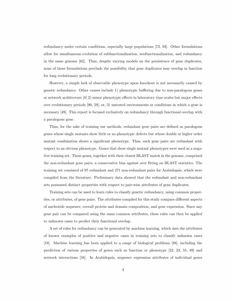
Preliminary analysis showed that select attribute values had distinct distributions between the

two groups. For example, BLAST E values were, in general, lower in the redundant pairs than

in the non-redundant pairs in the training set, indicating they share higher sequence similarity

(Figure 1.1a). A similar trend held for non-synonymous substitution rates between the two groups

4

(data not shown). Similarly, on average, gene pairs in the positive training set exhibited higher

expression correlation levels over the entire dataset (R=0.51) than gene pairs in the negative

training set (R=0.28). Thus, known redundant gene pairs appear to have a higher correlation

than gene pairs identified as non-redundant, as expected (Figure 1.1b). The disparate trends

in the two groups of gene pairs sets do not prove that all training set examples are correctly

labeled or that all gene pairs can be discretely labeled but it does indicate that the genes labeled

redundant, in general, show distinct attributes from those labeled non-redundant. Thus, there

is a basis for asking whether combinations of gene pair attributes could be used to improve the

prediction of genetic redundancy.

1.2.2 Algorithm Choice

Instead of predicting binary labels for genes pairs, machine learning methods can quantify re-

dundancy by posterior probabilities, which permit performance evaluation at different levels of

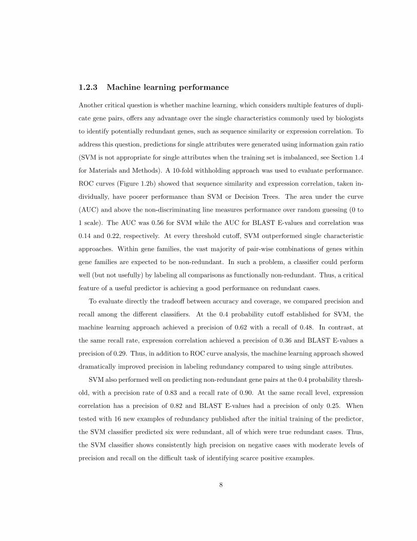
confidence. The Receiver Operating Characteristic (ROC) curve (Figure 1.2a), which plots true

vs. false positive rates at all possible threshold values, shows that SVM, Bayesian network, and

stacking (a combined method) performed better than decision trees, decision rules, or logistic

regression. All machine learning algorithms dramatically outperformed a random, or betting,

classifier (Figure 1.2a, diagonal line), which also supports the hypothesis that the training set la-

bels are not randomly assigned. SVM was used for further analysis because of its good empirical

performance and well-characterized properties [18].

The ROC curve analysis also permits an evaluation of an appropriate threshold for calling

redundant vs. non-redundant gene pairs. Using precision (true positive rate among positive

calls) and recall (true positives among positive calls vs. total true positives), the precision rate

increased relatively sharply from 0.2 to 0.4 probability. The rate then saturated after 0.4 while

recall dropped sharply after that point (Table 1.1). Thus, 0.4 was chosen as a balanced tradeoff

between true and false positives for further analysis of SVM.

5

(0, 1e−200]

(1e-200, 1e−150]

redundantnon−redundant

E−value Bins

Freq

uenc

y

0.0

0.1

0.2

0.3

0.4

(-0.4, −0.2]

redundantnon−redundant

Correlation Bins (R value)

Freq

uenc

y

0.00

0.05

0.10

0.15

0.20

0.25

0.30

(a)

(b)

(1e-150, 1e−100]

(1e-100,1e−50]

(1e-50,1]

(1, 10]

(-0.2, 0] (0, 0.2] (0.2, 0.4] (0.4, 0.6] (0.6, 0.8] (0.8, 1.0]

Figure 1.1: Frequency distribution of redundant vs. non-redundant pairs in the training set grouped

by (a) BLAST E-value (b) Pearson correlation of gene pairs in expression profiles across

the category All Experiments.

6

Probability Threshold

Recall Precision

0.2 0.79 0.4 0.21 0.78 0.4 0.22 0.75 0.41 0.23 0.74 0.42 0.24 0.72 0.43 0.25 0.7 0.44 0.26 0.69 0.45 0.27 0.67 0.46 0.28 0.65 0.47 0.29 0.64 0.49 0.3 0.62 0.51 0.31 0.61 0.52 0.32 0.6 0.55 0.33 0.59 0.55 0.34 0.56 0.56 0.35 0.55 0.56 0.36 0.54 0.58 0.37 0.52 0.58 0.38 0.51 0.6 0.39 0.49 0.61 0.4 0.48 0.62 0.41 0.47 0.63 0.42 0.46 0.64 0.43 0.45 0.65 0.44 0.43 0.65 0.45 0.41 0.66 0.46 0.4 0.67 0.47 0.38 0.68 0.48 0.37 0.68 0.49 0.35 0.7 0.5 0.35 0.7 0.51 0.33 0.71 0.52 0.31 0.71 0.53 0.29 0.72 0.54 0.27 0.72 0.55 0.25 0.72 0.56 0.24 0.74 0.57 0.23 0.74 0.58 0.21 0.74 0.59 0.2 0.74 0.6 0.19 0.76

Table 1.1: Trend in redundancy calls at varying probability thresholds.

7

1.2.3 Machine learning performance

Another critical question is whether machine learning, which considers multiple features of dupli-

cate gene pairs, offers any advantage over the single characteristics commonly used by biologists

to identify potentially redundant genes, such as sequence similarity or expression correlation. To

address this question, predictions for single attributes were generated using information gain ratio

(SVM is not appropriate for single attributes when the training set is imbalanced, see Section 1.4

for Materials and Methods). A 10-fold withholding approach was used to evaluate performance.

ROC curves (Figure 1.2b) showed that sequence similarity and expression correlation, taken in-

dividually, have poorer performance than SVM or Decision Trees. The area under the curve

(AUC) and above the non-discriminating line measures performance over random guessing (0 to

1 scale). The AUC was 0.56 for SVM while the AUC for BLAST E-values and correlation was

0.14 and 0.22, respectively. At every threshold cutoff, SVM outperformed single characteristic

approaches. Within gene families, the vast majority of pair-wise combinations of genes within

gene families are expected to be non-redundant. In such a problem, a classifier could perform

well (but not usefully) by labeling all comparisons as functionally non-redundant. Thus, a critical

feature of a useful predictor is achieving a good performance on redundant cases.

To evaluate directly the tradeoff between accuracy and coverage, we compared precision and

recall among the different classifiers. At the 0.4 probability cutoff established for SVM, the

machine learning approach achieved a precision of 0.62 with a recall of 0.48. In contrast, at

the same recall rate, expression correlation achieved a precision of 0.36 and BLAST E-values a

precision of 0.29. Thus, in addition to ROC curve analysis, the machine learning approach showed

dramatically improved precision in labeling redundancy compared to using single attributes.

SVM also performed well on predicting non-redundant gene pairs at the 0.4 probability thresh-

old, with a precision rate of 0.83 and a recall rate of 0.90. At the same recall level, expression

correlation has a precision of 0.82 and BLAST E-values had a precision of only 0.25. When

tested with 16 new examples of redundancy published after the initial training of the predictor,

the SVM classifier predicted six were redundant, all of which were true redundant cases. Thus,

the SVM classifier shows consistently high precision on negative cases with moderate levels of

precision and recall on the difficult task of identifying scarce positive examples.

8

False positive rate

True

pos

itive

rate

0.0 0.2 0.4 0.6 0.8 1.0

0.0

0.2

0.4

0.6

0.8

1.0

SVMC4.5PARTBayesNetLogisticStacking

False positive rate

True

pos

itive

rate

0.0 0.2 0.4 0.6 0.8 1.0

0.0

0.2

0.4

0.6

0.8

1.0

SVMC4.5All ExperimentsE−value

(a)

(b)

Figure 1.2: Receiver Operating Characteristic (ROC) curve for comparing (A) 5 different machine

learning algorithms and one meta-algorithm (StackingC); The hashed diagonal line is the

performance of a simple betting classifier, which represents probilistic classification based

on the frequency of positive and negative cases in the training set. (B) single-attribute clas-

sifiers using correlation of gene pairs across all microarray experiments (All Experiments)

and BLAST E-values

9

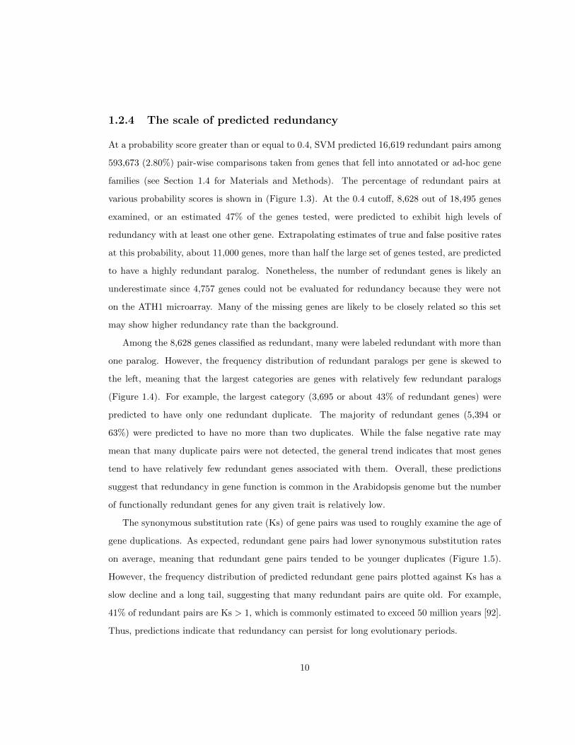
1.2.4 The scale of predicted redundancy

At a probability score greater than or equal to 0.4, SVM predicted 16,619 redundant pairs among

593,673 (2.80%) pair-wise comparisons taken from genes that fell into annotated or ad-hoc gene

families (see Section 1.4 for Materials and Methods). The percentage of redundant pairs at

various probability scores is shown in (Figure 1.3). At the 0.4 cutoff, 8,628 out of 18,495 genes

examined, or an estimated 47% of the genes tested, were predicted to exhibit high levels of

redundancy with at least one other gene. Extrapolating estimates of true and false positive rates

at this probability, about 11,000 genes, more than half the large set of genes tested, are predicted

to have a highly redundant paralog. Nonetheless, the number of redundant genes is likely an

underestimate since 4,757 genes could not be evaluated for redundancy because they were not

on the ATH1 microarray. Many of the missing genes are likely to be closely related so this set

may show higher redundancy rate than the background.

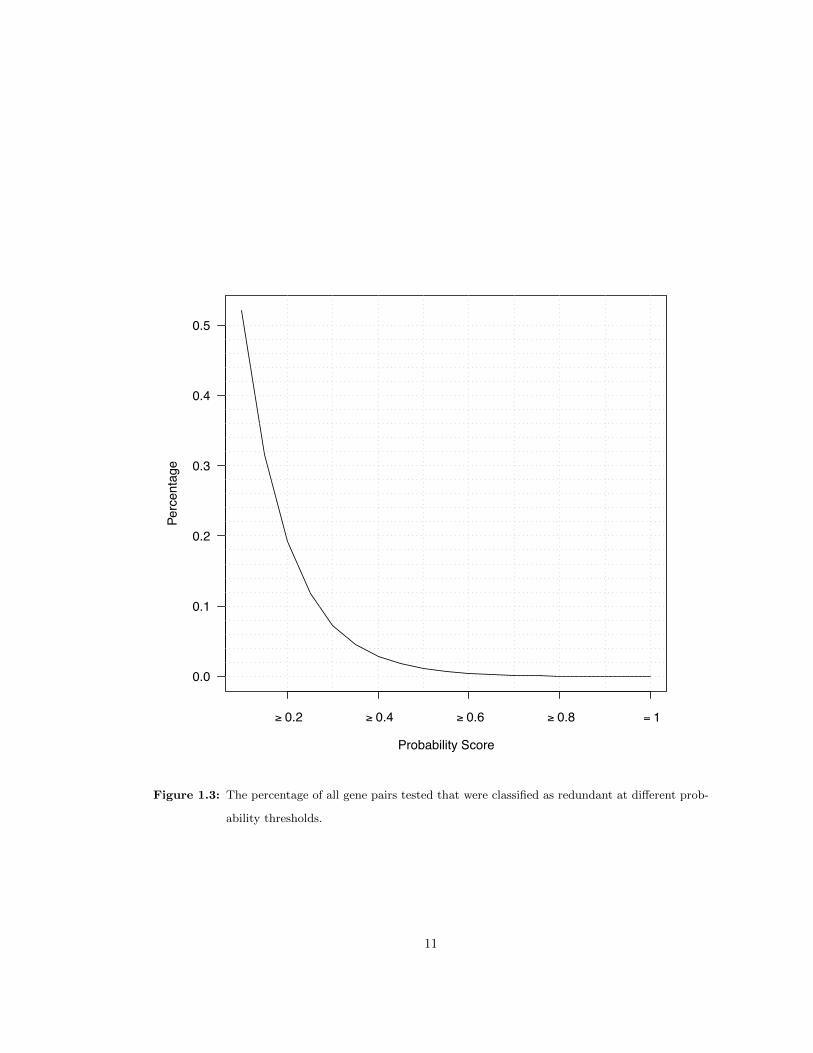
Among the 8,628 genes classified as redundant, many were labeled redundant with more than

one paralog. However, the frequency distribution of redundant paralogs per gene is skewed to

the left, meaning that the largest categories are genes with relatively few redundant paralogs

(Figure 1.4). For example, the largest category (3,695 or about 43% of redundant genes) were

predicted to have only one redundant duplicate. The majority of redundant genes (5,394 or

63%) were predicted to have no more than two duplicates. While the false negative rate may

mean that many duplicate pairs were not detected, the general trend indicates that most genes

tend to have relatively few redundant genes associated with them. Overall, these predictions

suggest that redundancy in gene function is common in the Arabidopsis genome but the number

of functionally redundant genes for any given trait is relatively low.

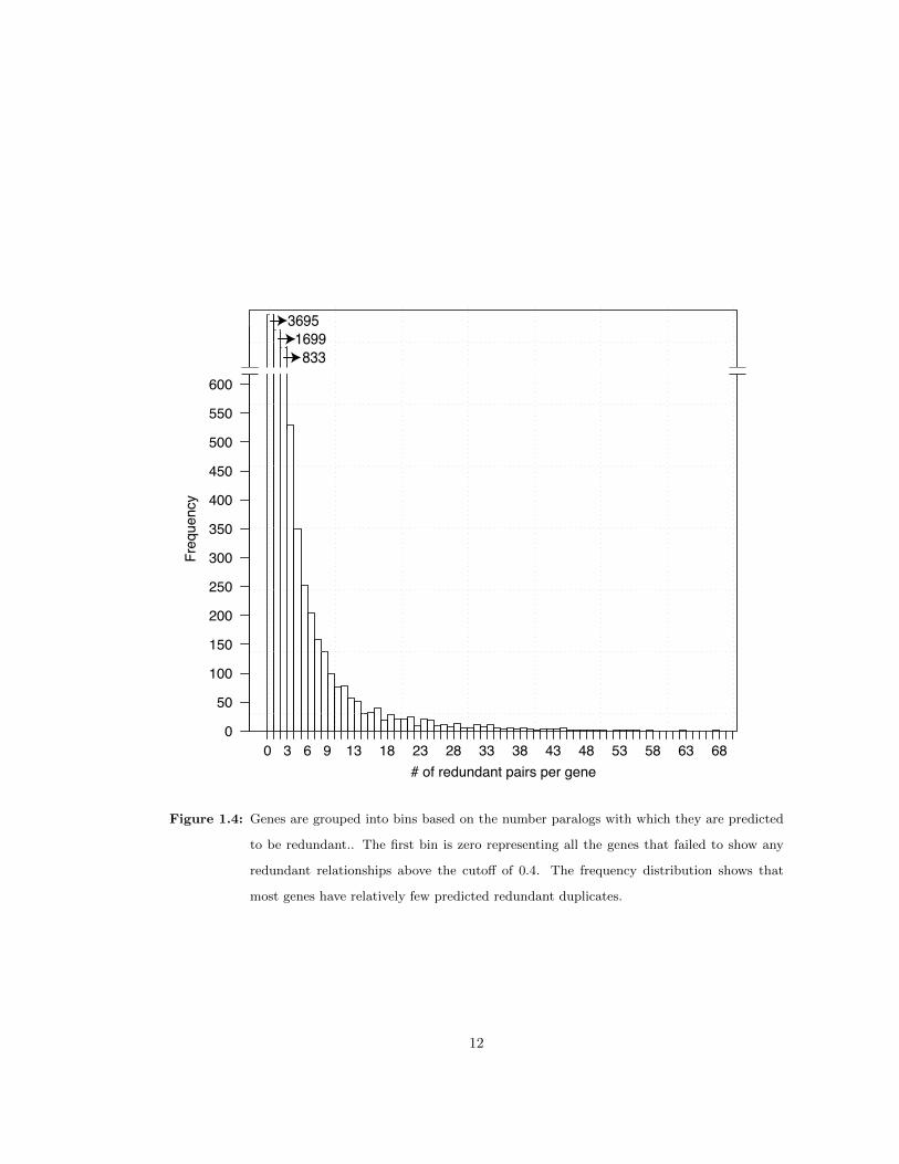
The synonymous substitution rate (Ks) of gene pairs was used to roughly examine the age of

gene duplications. As expected, redundant gene pairs had lower synonymous substitution rates

on average, meaning that redundant gene pairs tended to be younger duplicates (Figure 1.5).

However, the frequency distribution of predicted redundant gene pairs plotted against Ks has a

slow decline and a long tail, suggesting that many redundant pairs are quite old. For example,

41% of redundant pairs are Ks > 1, which is commonly estimated to exceed 50 million years [92].

Thus, predictions indicate that redundancy can persist for long evolutionary periods.

10

Probability Score

Perc

enta

ge

≥ 0.2 ≥ 0.4 ≥ 0.6 ≥ 0.8 = 1

0.0

0.1

0.2

0.3

0.4

0.5

Figure 1.3: The percentage of all gene pairs tested that were classified as redundant at different prob-

ability thresholds.

11

# of redundant pairs per gene

Freq

uenc

y

0 3 6 9 13 18 23 28 33 38 43 48 53 58 63 680

50

100

150

200

250

300

350

400

450

500

550

600

36951699833

Figure 1.4: Genes are grouped into bins based on the number paralogs with which they are predicted

to be redundant.. The first bin is zero representing all the genes that failed to show any

redundant relationships above the cutoff of 0.4. The frequency distribution shows that

most genes have relatively few predicted redundant duplicates.

12

[0,0.5)

redundantnon−redundant

Synonymous Substitution Rates (Ks) Bins

Freq

uenc

y

0.00

0.05

0.10

0.15

0.20

0.25

0.30

0.35

[0.5,1) [1,1.5) [1.5,2) [2,2.5) [2.5,3) [3,3.5) [3.5,4) [4,4.5) [4.5,5)[5,200)

Figure 1.5: Frequency distribution of redundant vs. non-redundant pairs in the training set grouped

by intervals of Ks values.

13

1.2.5 How attributes contribute to predictions

Given that multiple attributes improve the predictability of redundancy, we asked which at-

tributes contribute most to predictions. Two measures were used to assess the informativeness

of individual attributes on SVM predictions: 1) the absolute value of SVM weights, which are

the coefficients of the linear combination of attributes that is transformed into redundancy pre-

dictions (see Section 1.4 for Materials and Methods), and, 2) SVM sensitivity analysis in which

single attributes were removed and the overall change in predictions was quantified (using corre-

lation of probability values compared to the original SVM predictions). The two analyses were

largely in agreement in identifying the top ranking attributes (online supplemntary file) and an

average of the two ranks was used as a summary rank.

Several unexpected attributes ranked highly in the analysis, suggesting that functional infor-

mation on gene pair divergence could be captured by attributes that are rarely utilized. The

highest ranking attribute was isoelectric point (Rank 1), which measures a difference in the pH

at which the two paralogs carry no net electrical charge. Thus, the measure is sensitive to differ-

ences in the balance of acidic and basic functional groups on amino acids, potentially capturing

subtle functional differences in protein composition. Similarly, Molecular Weight ranked fifth.

An index of the difference in Predicted Protein Domains ranked seventh, apparently providing

functional information on the domain level.

It was noteworthy that typically summary statistics on protein or sequence similarity did not

rank highly. For example, BLAST Score (Rank 17), E-value (Rank 23), and Non-Synonymous

Substitution Rate (Rank 28) were not among the top ranking attributes, although preliminary

analysis showed they contained some information pertaining to redundancy. The low contri-

bution of these attributes was partly due to the fact that gene pairs were already filtered by

moderate protein sequence similarity (BLAST E-value of 1e-4, see Section 1.4 for Materials and

Methods) but this cutoff is relatively non-stringent. Thus, measures that capture changes in

protein composition like isoelectric points or predicted domains appear more informative about

redundancy at the family level than primary sequence comparisons.

For gene expression, two types of experimental categories had a high rank for predictions,

those that contained many experiments and those that examined expression at high spatial res-

14

olution. In the first category, All Experiments” (Rank 4), ”Pathogen Infection Experiments”

(Rank 6), and ”Genetic Modification Experiments” (Rank 7) were among the top ranked cate-

gories. These categories all shared the common feature of being among the largest, comprised

of hundreds of experiments each (Table 1.2). Thus, large datasets appear to sample enough

expression contexts to reliably report the general co-expression of two paralogs for redundancy

classification. The specific experimental context may also carry information.

In contrast to providing information over a broad range of experiments, tissue and cell-type

specific profiles had relatively few experiments but appeared to provide useful information on

fine spatial scale. For example, ”Root Cells, which is a compendium of expression profiles from

cell types [9, 14], ranked 2nd for all attributes. At organ level resolution, ”Organism Part”

ranked 11th[84]. Similarly, the large-scale and spatially resolved expression data sets were not

highly correlated to each other (e.g., Pathogen Infection and Root Cells, R=0.19). Thus, while

attributes are not completely independent, they appear to provide different levels of information

that machine learning can use to create a complex signature to identify redundancy.

1.2.6 Functional trends in predicted genome-wide genetic redundancy

The ability to identify redundancy at reasonable accuracy across the genome permits an analysis

of genome-wide trends in the divergence of gene pairs. Gene Ontology was used to ask whether

certain functional categories of genes were more likely to diverge or remain redundant according

to predictions. To control for the number of closely related genes, paralogous groups of genes

were binned into small (< 5), medium (≥ 5,≤ 20,) or large (> 20) classes based on the number of

hits with a BLAST cutoff of 1e-4 or less. In each class, gene pairs were split into redundant and

non-redundant categories and each group was analyzed for over-represented functional categories

(see Section 1.4 for Materials and Methods).

We focused analysis on signal transduction since such genes are the frequent targets of re-

verse genetics and distinct trends in these categories emerged from the data. Within this large-

sized paralog group, non-redundant genes were over-represented in the category of regulation

of transcription (p< 10−6, 301 genes, online supplementary file). These included members of

the AP2-EREBP (52), basic Helix-Loop-Helix (33), MYB (35), MADS-box (18), bZIP (16), and

15

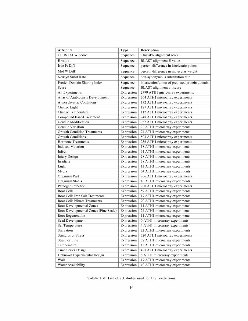
Attribute Type Description CLUSTALW Score Sequence ClustalW alignment score E-value Sequence BLAST alignment E-value Isoe Pt Diff Sequence percent difference in isoelectric points Mol W Diff Sequence percent difference in molecular weight Nonsyn Subst Rate Sequence non-synonymous substitution rate Protien Domain Sharing Index Sequence intersection/union of predicted protein domain Score Sequence BLAST alignment bit score All Experiments Expression 2799 ATH1 microarray experiments Atlas of Arabidopsis Development Expression 264 ATH1 microarray experiments Atmosphereric Conditions Expression 172 ATH1 microarray experiments Change Light Expression 127 ATH1 microarray experiments Change Temperature Expression 112 ATH1 microarray experiments Compound Based Treatment Expression 248 ATH1 microarray experiments Genetic Modification Expression 952 ATH1 microarray experiments Genetic Variation Expression 22 ATH1 microarray experiments Growth Condition Treatments Expression 74 ATH1 microarray experiments Growth Conditions Expression 503 ATH1 microarray experiments Hormone Treatments Expression 256 ATH1 microarray experiments Induced Mutation Expression 18 ATH1 microarray experiments Infect Expression 61 ATH1 microarray experiments Injury Design Expression 28 ATH1 microarray experiments Irradiate Expression 28 ATH1 microarray experiments Light Expression 12 ATH1 microarray experiments Media Expression 54 ATH1 microarray experiments Organism Part Expression 806 ATH1 microarray experiments Organism Status Expression 16 ATH1 microarray experiments Pathogen Infection Expression 200 ATH1 microarray experiments Root Cells Expression 59 ATH1 microarray experiments Root Cells Iron Salt Treatments Expression 17 ATH1 microarray experiments Root Cells Nitrate Treatments Expression 20 ATH1 microarray experiments Root Developmental Zones Expression 11 ATH1 microarray experiments Root Developmental Zones (Fine Scale) Expression 24 ATH1 microarray experiments Root Regeneration Expression 11 ATH1 microarray experiments Seed Development Expression 6 ATH1 microarray experiments Set Temperature Expression 4 ATH1 microarray experiments Starvation Expression 22 ATH1 microarray experiments Stimulus or Stress Expression 320 ATH1 microarray experiments Strain or Line Expression 32 ATH1 microarray experiments Temperature Expression 15 ATH1 microarray experiments Time Series Design Expression 427 ATH1 microarray experiments Unknown Experimental Design Expression 8 ATH1 microarray experiments Wait Expression 17 ATH1 microarray experiments Water Availability Expression 40 ATH1 microarray experiments

Table 1.2: List of attributes used for the predictions

16

C2H2 (10) transcription factor families (online supplementary file). Similarly, in the small-sized

families, the same term was also over-represented among non-redundant genes (p< 0.01) with

subgroups of many of the same gene families mentioned above. In the large gene family class, the

frequency of transcriptional regulators with at least one redundant paralog was only 30% com-

pared to a background of all genes with 50%. Similar trends were observed in the distribution

of predicted probabilities of redundancy, with transcription factors skewed toward lower values

(Figure 1.6a)

We examined the average values of attributes among redundant and non-redundant pairs

to ask how attribute values contributed to classifications. On the gene expression level, gene

pairs in the transcriptional regulator category showed a distribution of correlation values that

was skewed toward lower values (e.g., Figure 1.6b,c). For sequence attributes, transcriptional

regulator gene pairs also showed higher differences in isoelectric points compared compared to

all genes in large family size class (Figure 1.6d). In summary, transcriptional regulators in large

gene family classes show a trend of gene pair functional divergence, with tendencies to diverge

in expression pattern and in subtle protein properties.

In contrast, genes predicted to be redundant were dramatically over represented in kinase

activity, another category of signal transduction (p< 10−51, 817, online supplemntary file). The

term included many members of the large receptor kinase-like protein family (online supplemen-

tary file). The distribution of redundancy probability for gene pairs in the kinase category was

skewed toward higher values compared to all genes in the same large family class (Figure 1.6a).

In contrast to the transcriptional regulator category, about 85% percent of kinases had at least

one predicted redundant paralog. In general, the redundant kinases show the typical trends of

redundant genes from other categories, with high correlation over a broad set of experiments

(Figure 1.6b,c). Interestingly, despite the high level of predicted redundancy, gene pairs in the

kinase category also showed a high divergence in isoeletric points (Figure 1.6d), showing that

this attribute trend of kinases, which typically signified non-redundancy, was overcome by other

attributes. Overall, redundancy analysis suggests that genes at different levels of signal trans-

duction show distinct trends in redundancy, which has intriguing implications for the general role

of different signaling mechanisms in evolutionary change.

It is important to note that not all attributes showed the same trends in each functional

17

0.2

0.4

0.6

0.8

1.0

Prob

abilit

y Sc

ore

0.2

0.4

0.6

0.8

1.0

Cor

rela

tion

of A

ll Ex

perim

ents

0.2

0.4

0.6

0.8

1.0

Roo

t Cel

ls N

itrat

e Tr

eatm

ents

0.2

0.4

0.6

0.8

1.0

Isoe

lect

ric P

oint

Diff

.

kinase activity all regulationof transcription

kinase activity all regulationof transcription

kinase activity all regulationof transcription

kinase activity all regulationof transcription

(a) (c)

(b) (d)

Figure 1.6: Box and whisker plots show landmarks in the distribution of values, where the horizontal

line represents the median value, the bottom and top of the box represent the 25th and

75th percentile values, respectively, and the whisker line represents the most extreme value

that is within 1.5 interquartile range from the box. Points outside the whisker represent

more extreme outliers. The category all represents all genes in the large size class (see text)

and is used as a background distribution. The two other categories represent genes in the

GO functional category named.

18

category. For example, other functional categories with redundant genes showed different trends

in attributes relative to the background, as noted above for the isoeletric point attribute for

kinases. This means that the attributes display some independence and machine learning can

rely on different attributes to call redundancy in different genes.

1.2.7 Duplication Origin and Predicted Redundancy

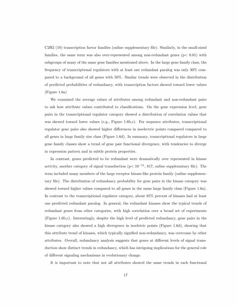
We also asked whether there were trends in redundancy stemming from either single or large-

scale duplication events. To compare redundancy trends by duplication origin, gene pairs were

labeled according to previous genome-wide analyses that identified recent segmental duplication

events in Arabidopsis [12] as well as tandem and single duplications [10]. To minimize bias that

might be caused by a correlation with the age of a duplication event, only gene pairs with a

synonymous substitution rate (Ks) below 2 were used. The cutoff, in addition to the fact that

many very recent duplicates were not included on the microarray and could not be analyzed,

made the distribution of Ks values in recent and single duplication events highly similar (Figure

1.7ab). Thus, the comparison of these two groups was not confounded by differences in the

apparent ages of duplication events in the recent segmental vs. single duplication events.

The average probability of redundancy was significantly higher among gene pairs in the most

recent duplication event than among gene pairs resulting from single duplication events (0.47

vs. 0.28, p< 10−15 by t-test). Despite the equilibration of neutral substitution rates, gene

pairs in the two groups differed dramatically, on average, in molecular weight difference (0.04

recent vs. 0.13 single) and isoelectric point difference (0.8 recent vs. 0.12 single). In addition,

expression correlation between gene pairs was generally two-fold higher in recent duplicates than

in single duplication events. Higher predicted redundancy among segmental duplicate pairs was

not trivially due to larger gene families in that class, as the number of closely related genes for

gene pairs in the single, old, recent, and tandem events is 54, 7, 20, and 46, respectively. It is

possible that synonymous substitution rates do not accurately reflect relative divergence times

but it is not apparent how one group would show bias over the other. Thus, the predictions

suggest that duplicates from large segmental duplications diverge more slowly in function, as is

evident in low divergence in expression and protein-level properties.

19

0.0 0.5 1.0 1.5

02

46

8

Synonymous Substitution Rates (Ks)

Perc

enta

ge o

f dup

licat

ion

even

ts

recentsingletandemold

−0.5 0.0 0.5 1.0

01

23

45

6

Correlation of Expression

Perc

enta

ge o

f Dup

licat

ion

Even

ts

recentsingletandemold

(a)

(b)

Figure 1.7: Frequency distribution of large-scaled duplication events (recent and old), as well as single

and tandem duplications grouped by (a) Synonymous Substitution Rates (Ks) (b) Pearson

correlation of gene pairs in expression profiles across the category All Experiments.

20

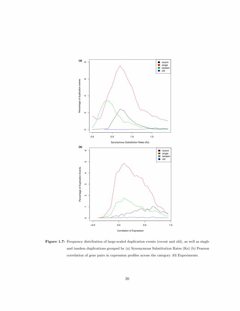
1.2.8 An online web interface to query redundancy predictions

The genome-wide predictions generated here can be accessed at http://redundome.bio.nyu.

edu. The interface permits users to enter a gene of interest and the website will return a similarity

tree based on ClustalW alignment score [56] scores. Redundancy predictions are mapped onto

the tree (Figure 1.8). The similarity tree consists of annotated members of the gene family

from The Arabidopsis Information Resource (TAIR) [82]. When the gene is not a member of an

annotated gene family, a tree is displayed for the 19 genes with closest BLAST E-values to the

query gene. The query gene appears in red and all redundant genes at or above the 0.4 cutoff

appear in green. In many cases, the paralogs with the highest predicted redundancy are not the

most similar in sequence. Mousing over a particular gene in the tree will display the pair-wise

attributes between the query gene and the subject displayed in the tree. Genes predicted to be

redundant that are more distantly related will appear on a separate list on the right. All the

information can also be displayed in tabular format. Some users may be particularly interested in

the potential for redundancy among a specific set of experiments as genes may show redundancy

in some functions and not others [15]. Thus, we have generated predictions based on specific

subsets of the expression data compendium, where analysis is performed on a relevant subset of

expression data and all sequence attributes. Radio buttons at the top of the page enable users to

pick from various attribute categories. The default All category includes all attributes on which

the evaluation in this report is based.

1.3 Conclusions

Identifying redundancy is a complex problem in which gene pairs may be redundant in some

phenotypes but not others. However, the results indicate that there is enough generality in the

outcome of gene duplication to classify redundancy based on evidence from disparate phenotypes.

Among the gene pairs that the SVM classified as redundant, 62% were correct in withholding

analysis. At this level of precision for redundancy predictions, SVM was able to correctly label

48% of all known cases of redundant gene pairs. The best single attribute classifier achieved a

precision of only 36% at a cutoff that correctly labeled 48% of known cases of redundancy. The

21

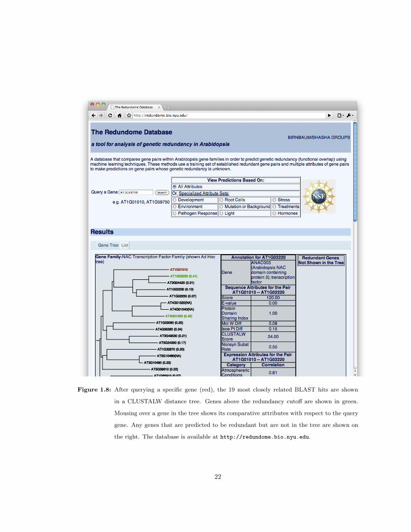
Figure 1.8: After querying a specific gene (red), the 19 most closely related BLAST hits are shown

in a CLUSTALW distance tree. Genes above the redundancy cutoff are shown in green.

Mousing over a gene in the tree shows its comparative attributes with respect to the query

gene. Any genes that are predicted to be redundant but are not in the tree are shown on

the right. The database is available at http://redundome.bio.nyu.edu.

22

ROC curve analysis showed that no single attribute classifier performed better than SVM at any

point in the analysis of true positive vs. false positives. Overall, machine learning performance

was about twice as high as single attribute methods. The ability to predict redundancy at

reasonable precision and recall rates constitutes a resource for studying genome evolution and

redundancy in genetics.

1.3.1 Informative attributes

The strength of the machine learning approach is that it can take advantage of multiple types of

information and give each type a different weight. While more than 40 attributes were used in the

analysis, the effective number of gene pair attributes was likely much smaller due to correlations

among attributes. However, four or five distinct sets of attributes showed low correlation to each

other and were shown to be informative for classification.

Among attributes related to sequence composition, the most informative were not those typ-

ically used to assess genetic redundancy. The highest ranking attribute was an index of the

difference in isoelectric points. The fifth highest ranking attribute was an index of the differ-

ence in molecular weight. An index of predicted domain sharing also ranked highly, largely

because results were sensitive to its removal from the machine learning process, indicating that

it provided relatively unique information. It was surprising that BLAST E-values provided little

information at values lower than 1e-4, the cutoff for the pairwise comparisons. This implies that,

within gene families, other measures such as changes in the charge composition of proteins or

alterations in the domain structure are better indicators of functional redundancy than direct

sequence comparison metrics.

Two types of expression-based attributes were informative, including those comprised of many

experiments and those that resolved mRNA localization into specific tissues or transcriptional

response to an environmental stimulus. While the large expression datasets were highly correlated

(e.g., Genetic Modification and Organism Part, R=0.81), they were much less correlated with

the high resolution data (e.g., Root Cells and Genetic Modification, R=0.30). Thus, it appears

that different types of expression data are contributing at least some distinct information, with

high spatial resolution datasets providing informative contextual information and larger datasets

23

tracking the broad behavior of duplicate genes.

1.3.2 Functional trends in redundancy

Genes annotated with roles in transcriptional regulation, including many transcription factors,

showed a tendency toward functional divergence. The opposite trend occurred at another level of

signal transduction with kinases showing a tendency toward redundancy. Interestingly, divergent

redundant transcriptional regulators showed, on average, a divergence in isoelectric points com-

pared to the background or even other redundant categories. This global trend fits arguments,

based on case studies, that modular changes in transcription factor proteins are plausible mech-

anisms for evolutionary change [94]. For example, it has been postulated that subtle changes

in proteins such as insertion of short linear motifs that mediate protein-protein interactions and

simple sequence repeats of amino acids could play a role in functional divergence of transcription

factors outside of dramatic changes to the DNA binding site[97, 70]. Still, a more systematic

examination of protein interactions among transcription factors is needed to corroborate these

findings. In general, the ability to classify large groups of genes enables an analysis of the

functional trends that shape redundancy in a genome.

1.3.3 Implications for Genome Organization

The high level of redundancy predicted in this study is in accordance with low hit rates in reverse

genetic screens in Arabidopsis and the high number of studies that have shown novel phenotypes

in higher order mutants. However, the estimated redundancy rates still leave room for other

explanations to account for the lack of single mutant phenotypes. For example, the machine

learning approach predicted that 50% of genes are not buffered by paralogous redundancy but

reverse genetic screens rarely achieve such a high rate of phenotype discovery. The predicted

redundancy rate may be an underestimate, as about 23% of all gene pairs identified in the study

could not be analyzed. Still, one implication of our results is that other prevalent phenomenon

are likely to buffer gene function including, for example, network architecture or non-paralogous

genes. Machine learning could eventually be applied to these other forms of redundancy but a

comprehensive training set for these phenomena is currently lacking.

24

While the machine learning approach predicted that half the genes in the genome had a

redundant paralog, most genes had no more than two other highly redundant paralogs. This

leads to the paradoxical conclusion that, while the function of many or even most genes is

buffered by a redundant paralog, redundancy is a relatively rare outcome of gene duplication. In

addition, the forces that shape redundancy appear to be complex and not strictly a function of

time. For example, a large proportion of predicted redundant gene pairs were quite ancient in

their origin. And, the mode of duplication, by either single or large segmental duplication, also

strongly influenced the tendency for gene pairs to diverge, according to predictions. Together,

these findings suggest that redundancy between pairs is a relatively rare but targeted phenomenon

with complex causes, including mode of duplication, time, and gene function.

1.3.4 Implications for Genetic Research

From a practical standpoint, SVM predictions still carry enough uncertainty of false positive and

false negative calls that they should be considered a guide to be used with researcher knowledge

rather than a certain prediction. We envision that geneticists who are already interested in con-

ducting reverse genetic studies of a gene of interest will often want to explore the possibility of

redundancy within the same gene family. The gene of interest can then be queried in our pre-

dictions to first evaluate the number of predicted redundant genes. A large number of predicted

redundant genes may be grounds for prioritizing another gene. If a small number of gene family

members are implicated in redundancy and single mutants fail to display a genotype, researchers

can use predictions to guide the construction of double or higher mutants. Quite often the most

sequence-similar gene is not the one predicted to most likely be redundant.

In the future, predictions can be improved by having more training data to learn redundancy

in more narrowly defined phenotypes. In addition, a more objective and quantitative definition

of redundancy would likely improve the quality of the training set. For example, the set of

downstream targets for transcription factors could provide a standardized quantitative measure

for single and double mutant phenotypes. These types of data would require significant work from

any individual research group. However, the training set is continuously under expansion due

to the efforts of the genetic research community as a whole. Studies investigating direct targets

25

of transcription factors are also increasingly common. Thus, the predictions of the machine

learning approach will improve over time. We view this report as a first generation approach

to exploring the genome-wide outcomes of gene duplication using machine learning approaches,

where reasonable estimates are now feasible.

1.4 Materials and Methods

1.4.1 Defining Gene Families

We used gene family annotations available through The Arabidopsis Information Resource (TAIR)

[82] which included 6,507 genes in 989 families. To group genes that were not annotated into

gene families in TAIR, we established ad-hoc gene families, in which all members had at least

one member in the family with a protein-protein BLAST E-value of 1e-4 and no members appear

in the annotated families. Among genes for which we generated predictions, there were a total of

17,158 genes grouped into ad-hoc gene families. We did not make predictions on the singletons

or genes lacking a probe on the ATH1 microarray. Thus, these genes were removed from the

analysis. After this step, there were 5,644 genes in the annotated families and 12,851 genes in

the ad hoc gene families.

1.4.2 Attribute Data Sources and Comparative Measures

For expression based characteristics, we downloaded all available microarray experiments from

Nottingham Arabidopsis Stock Centre (NASC) [26] for the ATH1 microarray. We further par-

titioned these experiments using the categorical ontology developed by NASC using the MGED

classification as found in the Treeview section in NASC. If two or more partitions overlapped

by more than 50 percent, we eliminated the smaller partition. We created additional partitions

using data from several different cell type-specific profiling experiments [9, 69, 57], root develop-

mental zones [9], fine-scale root developmental zones [14], dynamic profiling of root cells under

treatment with nitrogen [43], and root cells responding to abiotic stress [29]. Pearson correlation

was used to compare gene expression of gene pairs in each partition separately.

For sequence based attributes, we used TAIR protein sequence to generate pairwise attributes

26

for gene duplicates on protein BLAST E-value, BLAST scores, and ClustalW alignments[56].

We also calculated non-synonymous substitution rates using PAML [96]. The predicted domain

sharing index was based on the intersection/union of predicted domains for each protein pair,

where predicted domains for each protein were downloaded from TAIR. We also used percent

difference in isoelectric points where values for each protein were downloaded from TAIR. To

remove redundant attributes, we manually selected the subset in which all the pair-wise Pearson

correlations between attributes in the subset are lower than 0.85.

For the on-line database, predictions were derived from either using all attributes or subsets

of the data for assessing redundancy in specific biological contexts. When subsets of the data

were used, all sequence attributes were used but in combination with only sets of microarray

data that corresponded to biological categories, such as stress, hormone treatment, root cell type

expression profiles, or light manipulation.

1.4.3 Description of Machine Learning Programs

We tested six different machine-learning programs and selected Support Vector Machine (SVM)

for detailed analysis, based on the principle of Occam’s razor [30]. All programs were compared

using Wekas implementation [95]. For SVM, we used Wekas wrapper for LibSVM [20] for per-

formance evaluation but used LibSVM directly when predicting functional overlap. Below is a

brief summary of each:

Decision trees involve creation of a tree (often bifurcating) in which each tree node specifies

an attribute and a threshold to choose a decision path. A particular instance of the data (e.g.

gene pair) is mapped starting from the root and proceeding until a leaf is reached. Each leaf

contains a specific label (e.g. overlapping or non-overlapping function). At each node in the deci-

sion tree, the gene pair is interrogated about its value on a specific attribute (such as expression

correlation in a particular experiment). Thus, the path through the tree depends on the specific

attributes of the gene pair. We used Weka’s C4.5 [81] implementation to generate the decision

tree from the training set. For each attribute, the algorithm selects the threshold that maxi-

mally separates the positive and negative instances in the training set by using the information

gain measure. Therefore, decisions are taken sequentially until a terminal leaf is reached. The

27

label of the leaf is determined by the majority rule of labels from the training set. We set the

PruningConfidenceFactor to 0.25 (to address overfitting in the training set) and minNumObj to

2.

Decision rules specify conditions that must simultaneously be satisfied in order to assign a

label. Given a list of decision rules, these rules are tested sequentially until a label is assigned, or

otherwise the default label applies [80]. PART [38] was used to learn the decision rules from the

training set. It learns a rule by building a decision tree on the current subset of instances, con-

verting the path from root to the leaf that covers the most instances into a rule. It then discards

the tree, removes the covered instances, and learns the next rule on the remaining instances. We

used Wekas implementation of PART with the parameters PruningConfidenceFactor set to 0.25

and minNumObj set to 2.

Bayesian network is a generalized graphical model that assigns probabilities to specific labels.

Bayesian networks model conditional dependencies as the network topology: in this network,

attributes and the label are modeled as nodes and their conditional dependencies are specified

by directed edges. Each node also stores a probability table conditioned on its child nodes. The

probability for a label is proportional, based on Bayes rule, to the joint probability density func-

tion of all attributes and the label, which is further decomposed into the product of conditional

probability of each node given its parents. We used K2 [24] to learn the network structure. It

employs a hill-climbing strategy to iteratively refine the network structure by adding directed

edges and maximizing the likelihood such that it best describes the training data. We used Wekas

implementation of K2 with the parameter MaxNrOfParent set to 1, which essentially restricts

the learned network to be Naive Bayes [52].

Logistic regression uses a statistical model that assumes a linear relationship among attributes

[19]. It uses the logistic function that relates the linear combination of attributes to the prob-

ability of the label. One way to learn the coefficients in the linear equation is to maximize the

log-likelihood function that estimates the fitness between the predicted probability and the actual

label specified in the training data. We used Wekas implementation and default parameters.

Stacking (StackingC) [86] is a meta algorithm, which makes prediction by combining the

predictions from the participating machine learning algorithms. StackingC employs a linear

regression scheme to merge the predictions: the final predicted probability of a label is the linear

28

combination of the probabilities predicted by participating algorithms; in other words, it is a

weighted average of predictions where the weights for participating algorithms were learned from

the training set through a nested cross-validation process. We used Wekas implementation of

StackingC to combine predictions from decision trees, decision rules, Bayesian network, logistic

regression, and SVM.

Support vector machine (SVM) predicts the label of each instance by mapping it into a data

point in a high dimensional space, whose coordinates are determined by the values of attributes

[25]. The hyperplane is learned from the training set such that it separates instances with different

labels and also maintains the maximum margin to the nearest data points. A test case is then

labeled functionally overlapping or non-overlapping depending on which side of the hyperplane

it falls. One important property of maximum margin is that the error rate, when generalized to

all the data points from the sample space, is mathematically bounded. Furthermore, through

the use of a kernel function, points can be transformed non-linearly into a higher or even infinite

dimensional space where a better separating hyperplane might exist. We used LibSVM [20] with

linear kernel and default parameters. Attributes were normalized to [0,1] before learning and

prediction.

Platts probabilistic outputs for SVM provide a quantitative way for the confidence of redun-

dancy predictions [79]. This calibrated posterior probability for the redundancy label is based on

the distance from each data point to the hyperplane: larger distances on the redundant side of

the hyperplane result in larger probabilities, and similarly, larger distances on the non-redundant

side of the hyperplan lead to smaller probabilities for the redundant label. LibSVM rescaled

these distances and then transformed them by a sigmoid function into probabilistic measures.

We chose the linear kernel because its performance was similar to Radial Basis Function and

better than polynomial kernel with higher degrees in the withholding analysis (data not shown).

This might be due to the large number of attributes (43) but relatively fewer training instances

(368), as in [39]. Another advantage of using linear kernel is that it provides an intuitive way

to look at how attributes contribute to predictions: the separating hyperplane is simply a linear

combination of attributes. In other words, the predicted redundancy probability, which is based

on the distance to the hyperplane, is derived from the sum of the weighted attributes. Therefore,

we used the absolute values of the weights of attributes to assess the informativeness of attributes.

29

1.4.4 SVM Sensitivity Analysis

We used Pearson correlation of the predicted probabilities before and after removing single at-

tributes to quantify the sensitivity of single attributes when they were removed during the ma-

chine learning process. First, a smaller subset of attributes were selected, as described in [45], to

ensure they are both informative (by finding attributes that maximize the correlation between

them and the redundancy label) and independent (by minimizing the inter-correlations among

the selected attributes). This step was necessary because the original set of attributes contained

redundant information, so removing any one of them was compensated by other attributes and

didnt change the predictions significantly. We used SVM to make predictions using this smaller

subset of attributes (19) and then compared with the predictions where each of the attributes

was removed from the subset in turn (online supplemntary file).

1.4.5 Description of Information Gain Ratio used on single attribute

classifier

Binary partitioning a single attribute by setting a fixed threshold value is the most straightforward

classification. Every gene pair with a greater attribute value can thus be predicted redundant (or

non-redundant), with the predicted probability corresponding to the ratio of redundant (or non-

redundant) pairs over the whole training set. We determined this threshold value by exhaustively

testing each possible value of the attribute and kept the one with the maximum information gain

ratio to the known label. C4.5 uses the same strategy to select and branch on the attribute

iteratively.

1.4.6 The Withholding Strategy

We used 10-fold stratified cross-validation to evaluate the performance of machine learning algo-

rithms. The original training set was first partitioned into 10 equal-sized subsets. For each fold,

a different subset was evaluated using the model learned from the other subsets. The overall per-

formance measures were tallied among all folds; therefore, the method evaluates every instance in

the training set. This procedure essentially reduces the variation in estimating the performance

30

by averaging out the bias caused by particular instances. The stratified sampling procedure also

reduces the variation by ensuring that the proportion of instances with different labels in each

bin is the same as the whole training set. We used two measures for evaluation: recall rate of a

particular label is the ratio of true positives over all known positives, and, precision rate is the

ratio of true positives over both true positives and false positive.

1.4.7 Gene Ontology (GO) Analysis

For analysis of over-represented GO terms among redundant and non-redundant genes, genes

were split into redundant or non-redundant sets for each size class (large, medium or small if

the number of closely related genes are > 20, between 5 and 20, or < 5, repectively, using

BLAST cutoff of 1e-4). This meant that large gene families were sometimes broken up into

more than one paralogous group, depending on how many closely related genes they had. We

calculated overrepresented GO terms for cellular component, biological process and molecular

function classification systems and then merged results. We then asked what GO terms were

over represented (P< 10−2) in each set for each size class. GO terms or their descendents were

used. We used Bioconductors GOstats package [41, 33] to find the overrepresented GO terms,

which derives p-values of over-represented GO terms based on the hypergeometric distribution.

We then examined average attributes for genes in each set that mapped to over-represented

categories.

31

2ContactBind

2.1 Background

The contact between transcription factors (TFs) and DNA binding sites is crucial to the expres-

sions of regulated genes and, thus, the phenotype of cells and organisms. One way to identify

the DNA binding motif of a single transcription factor is to find the over-represented binding

site among the set of promoters bound by the transcription factor. A variety of computational

methods such as MEME [3] or AlignACE [51] have been proposed and successfully have pre-

dicted DNA binding motifs [46]. These methods usually model binding motifs by position weight

matrices (PWMs), summarizing the frequency distributions of nucleotides in each position of

the binding site sequence. However, these methods predict only binding motifs from sets of

promoter sequences that are identified by experiments such as chromatin immunoprecipitation

(ChIP-chip). This limits the number of predicted binding motifs to the availability of transcrip-

tion factor binding experiments. The same limitation also applies to high-throughput sequencing

technologies, such as ChIP-seq, where short reads of sequences around the targeted binding sites

were extracted and sequenced, and mapped onto genomic locations by computational methods

[87].

One way to extend predictions of binding motifs beyond the current binding data is to use

the structural knowledge of TF-DNA binding complexes. Morozov et al. presented a biophysical

model to predict binding motifs by estimating binding free energy between contact residues and

binding sites, and converting the predicted energy into the binding motifs [67]. However, this

model is limited by the availability of biophysical measurements such as free binding energy, which

is scarce compared to the amount of binding data. Additionally, they can’t extend predictions

beyond prior binding data when they combined the data to improve accuracy [68].

Kaplan et al. took advantage of the structural knowledge that is specific to the zinc finger

family [76, 32] to learn amino acid-nucleotide recognition preferences from datasets of binding

experiments [54]. They focused on selected contact residues on the fingers, and learned how

residues on the contact positions recognize different nucleotides. Binding motifs of novel tran-

32

scription factors were predicted by looking up the learned recognition preferences by their contact

residues. However, their work requires an in-depth understanding of molecular interactions in

the binding complexes and, therefore, is currently limited to the zinc finger family only.

Here we will propose a novel method to predict binding motifs for transcription factors in var-

ious families and utilize both structural knowledge and datasets of binding experiments. Within

families, we assume that mutations of contact residues determine their DNA recognition, but

relax the requirement for prior knowledge about the specific contact positions. With the help of

familial binding datasets, we learned both the positions of contact positions in protein sequences,

and their amino acid-nucleotide recognition preferences. Therefore, we can infer the binding mo-

tif of a novel transcription factor by looking at its residues on contact positions and determined

corresponding nucleotides from the recognition preferences.

We used Bayesian networks, a generative graphical model, to encode both the positions of

contact residues in transcription factors and their amino acid-nucleotide recognition preferences.

Bayesian networks have been used to solve a variety of biological problems, such as reconstructing

regulatory networks from microarray expressions [77]. In this project, we used them in a different

way to model dependences between molecules on both sides of the binding interface.

We adopted a bipartite network structure, which includes disjoint sets of residue nodes (V1={AAn|n

: the position in protein sequences of transcription factors}) and nucleotide nodes (V2 ={DNAn|n

: the position in binding site sequences}). Each residue node is a random variable that describes

the occurrences of residues in a position within the protein sequences. Similarly, each nucleotide

node describes the occurrences of nucleotides in a position within the binding sites. Directed

edges model statistical dependences from the set of residue nodes to the other set of nucleotide

nodes (E={(u,v)| u ∈ V1 , v ∈ V2}), and were learned in a way such that the network struc-

ture best fits the dependences in the given dataset. In order to predict binding motifs of novel

transcription factors, the independent probability distributions of nucleotides on the nucleotide

nodes without incoming edges are converted to PWMs. Likewise, the conditional distributions

on the nucleotide nodes that depend on the residue nodes are resolved by looking up their parent

residues in the sequences of the novel TFs.

In this project, we predicted binding motifs and its locations in promoters for three structural

families: homeodomain, basic helix-loop-helix(bHLH), and MADS-box. Homeodomain is one of

33

the most common DNA-binding domains in eukaryotes, and its binding interactions have been

found to be conserved among species [40]. This domain consists of a N-terminal arm, followed by

three alpha-helices. The arm contacts with DNA in the minor groove and the third helix forms

hydrogen bonds with nucleotides in the major groove. The basic helix-loop-helix (bHLH) domain

is also a large family of transcription factors in eukaryotes. It is composed of two distinct but

neighboring sub-structures: a basic region on the N-terminal that contacts with DNA, followed

by a HLH sub-structure that forms a homo- or hetero- dimer with another bHLH-containing

protein [53, 64]. The third family, MADS-box [65], is a big family of transcription factors in

plant. In addition to form homo- or hetero- dimers with another MADS-box protein, it usually

involves in a ternary complex that recruits proteins from other families [66].

We made binding site predictions for three families of transcription factors in the genome

of three species, Arabidopsis thaliana, Mus musculus (mouse), and Saccharomyces cerevisiae

(yeast). These predictions, as well as the tools making the predictions, are freely available on

the ContactBind website, located at http://contactbind.bio.nyu.edu.

2.2 Results and Discussion

2.2.1 Homeodomain

Homeodomain is a well-characterized family with abundant binding information and serves well

for constructing our network [1]. Two research groups have conducted extensive experiments

to determine the binding affinity of most of the transcription factors in the family. They used

different experiment protocols on different species yet reached very similar results. Noyes et al.

experimented with all 84 homeodomains in D. melanogaster (fly) using a bacterial one-hybrid

system (B1H), which determines binding affinity of transcription factors insides E. coli [73] .

Berger et al. characterized 168 mouse homeodomains using protein binding microarrays, which

probed the target transcription factor using an array of DNA oligo-nucleotides [5].

We used both cross-validation and cross-dataset validation to evaluate the performance of

our method. For cross-validation on Noyes et al.’s binding data, we iteratively withheld parts of

the TF-DNA pairs from the training process but then used the withheld parts to validate the

34

learned network. This indicated a 3.5% error rate (see Section 2.4 for Materials and Methods).

We also performed cross-dataset validation by validating our predictions with Berger et al.’s

mouse binding data, using the model we learned from Noyes et al.’s fly binding data. This

validation showed an error rate of 21.6% (see Section 2.4 for Materials and Methods).

As expected, a class of incorrect predictions in the cross-dataset validation resulted from the

cross-species evolution of contact residues. For example, Rhox6 in mouse is orthologous to Rx

in fly and both transcription factors bind to the same binding site, TAATAA. However, we only

correctly predicted it for Rx using fly’s binding data. Upon a closer inspection of this incorrect

prediction of Rhox6, we found that the residue Arg, on AA50, never appeared in the fly dataset

that we used to construct the model. In this case, we replaced it with the closest one, Lys, in the

training set, based on the +3 score specified in the BLOSUM45 substitution matrix (see Section

2.4 for Materials and Methods). This substitution, however, led to the incorrect prediction. On

the other hand, we successfully predicted it for Rx based on the residue on AA50, Gln, which

is still evolutionarily related to Rhox6’s Arg with a +1 score in BLOSUM45. However, Gln was

not considered for the substitution for its lower score (+1) than Lys (+3). Another example

is Hoxa9 in mouse, whose nucleotide on DNA2 isn’t identified because the residue, Cys, on its

AA6 parent never appeared in the fly dataset, and no substitution with positive scores was

suggested by BLOSUM45. In general, generalization of our model in predicting binding motifs

on other species might be limited by the lack of variability in contact residues, and require more

cross-species and divergent binding data for better generalization.

We learned the network structure and the probability distributions of nucleotides or residues

using the binding data from Noyes et al., as shown in Figure 2.1 and in Figure 2.2. Several

previously reported contact points were reflected, such as AA50 and AA54 [50]. However, the

interaction between AA51 and DNA3 was not learned because AA51 contains only Asn and DNA3

contains mostly Ade - both of them lacked the variability to infer the statistical dependency.

Since the binding sites of homeodomains are usually reported to have 6 base pairs, from DNA1

to DNA6, the edges for DNA-1 and DNA7 were expected to be insignificant for binding affinity,

as indicated in their low-information probability distribution.

One surprising dependency is the edge from AA6 to DNA2. DNA2 would be Ade if AA6

is in the set of residues, Val or Ala, whereas DNA2 would be Gua if AA6 is in the other set

35

AA2 AA3 AA4 AA5 AA6 AA7 AA8 AA47 AA48 AA49AA50 AA52 AA54AA55

DNA−1DNA1DNA2 DNA3DNA4DNA5 DNA6 DNA7

Figure 2.1: Learned Bayesian network for homeodomain. The residues on the N-terminal arm of home-

odomain are positioned from AA2 to AA8, while the others (AA47-AA55) located on the

third helix. Binding sites for homeodomain families are about 6 base pairs long and are

positioned from DNA1 to DNA6.

of residues, Gly, His, Leu, or Arg. We didn’t find available crystal structures to elicit such

a contact interaction, while we knew from MSX1 MOUSE that AA6 makes contacts with the

DNA phosphate backbone between DNA3 and DNA4 [50]. However, 9 homeodomains containing

the latter set of residues (Gly, His, Leu, or Arg) on AA6 were previously classified to a subfamily

characterized by Gua on DNA2.

It’s also interesting that the absence of residues on contact points (represented by a dash ”-”)

did affect binding affinity. When we aligned sequences, proteins that underwent residue deletion

events were split and modeled by gaps on these deleted positions. In Figure 2.2, the distribution

of Pr(DNA5|AA50, AA5) indicated that DNA5 changed from Ade to Cys if the residue Lys was

on AA50 and the residue on AA2 was deleted. Since AA2 is located on the unstructured N-

terminal arm, its deletion usually does not change the fold significantly yet its change on binding

affinity might be an interesting topic for a mutagenesis study.

Noyes et al.’s complete binding data that covers all the homeodomains in fly’s genome enables

us to assess how well our method generalizes if given less training data. In Figure 2.3, the error

rate drops significantly to 4.8% when we randomly selected 50% of the dataset for training. This

36

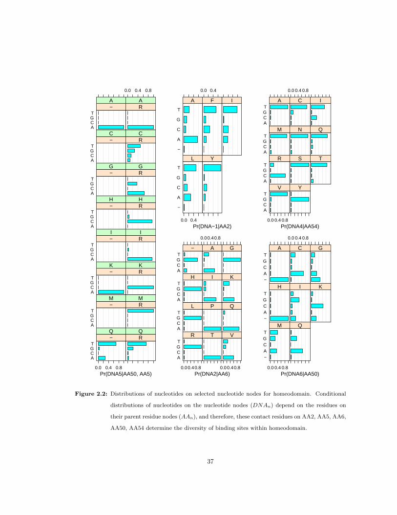
Pr(DNA6|AA50)

−ACGT

A

0.0 0.4 0.8

C G

−ACGT

H I K

−ACGT

0.0 0.4 0.8

M Q

Pr(DNA4|AA54)

ACGT

A

0.0 0.4 0.8

C I

ACGT

M N Q

ACGT

R S T

ACGT

0.0 0.4 0.8

V Y

Pr(DNA2|AA6)

ACGT

−

0.00.40.8

A G

ACGT

H I K

ACGT

L P Q

ACGT

0.00.40.8

R T

0.00.40.8

V

Pr(DNA−1|AA2)

−

A

C

G

T

A

0.0 0.4

F I

−

A

C

G

T

0.0 0.4

L Y

Pr(DNA5|AA50, AA5)

ACGT

−A

0.0 0.4 0.8

RA

ACGT

−C

RC

ACGT

−G

RG

ACGT

−H

RH

ACGT

−I

RI

ACGT

−K

RK

ACGT

−M

RM

ACGT

0.0 0.4 0.8

−Q

RQ

Figure 2.2: Distributions of nucleotides on selected nucleotide nodes for homeodomain. Conditional

distributions of nucleotides on the nucleotide nodes (DNAn) depend on the residues on

their parent residue nodes (AAn), and therefore, these contact residues on AA2, AA5, AA6,

AA50, AA54 determine the diversity of binding sites within homeodomain.

37

Percentage of Dataset

Err

or R

ate

10% 20% 30% 40% 50% 60% 70% 80% 90%

0.04

0.06

0.08

0.10

0.12

0.14

0.16

Figure 2.3: Generalization of the model on various sizes of subsets of the training set. The error rate

on each percentage of subsets of the training set was evaluated by repeating 30 selections

of subsets from Noyes et al.’s fly binding data.

suggests that the number of binding experiments could be reduced significantly while maintaining

similar performance, by taking advantage of the predictive power of our model.

We might reduce the number of binding experiments further by choosing subsets of transcrip-

tion factors that have higher variation of residues on contact positions. Conversely, even large

training sets that lacked variety showed a higher error rate (data now shown). Investigation of

this indicated that there is a small but significant set of TF-DNA pairs. While withholding this

set from learning, the error rates spiked. In fact, approximately half of homeodomain binding

sites in fly’s genome are reported similar [1], suggesting the importance of such a small set in our

learning. Therefore, carefully choosing TFs with divergent contact residues is beneficial to the

generalization of our model.

We predicted PWMs and their binding locations in promoters in the genome of Arabidopsis

38

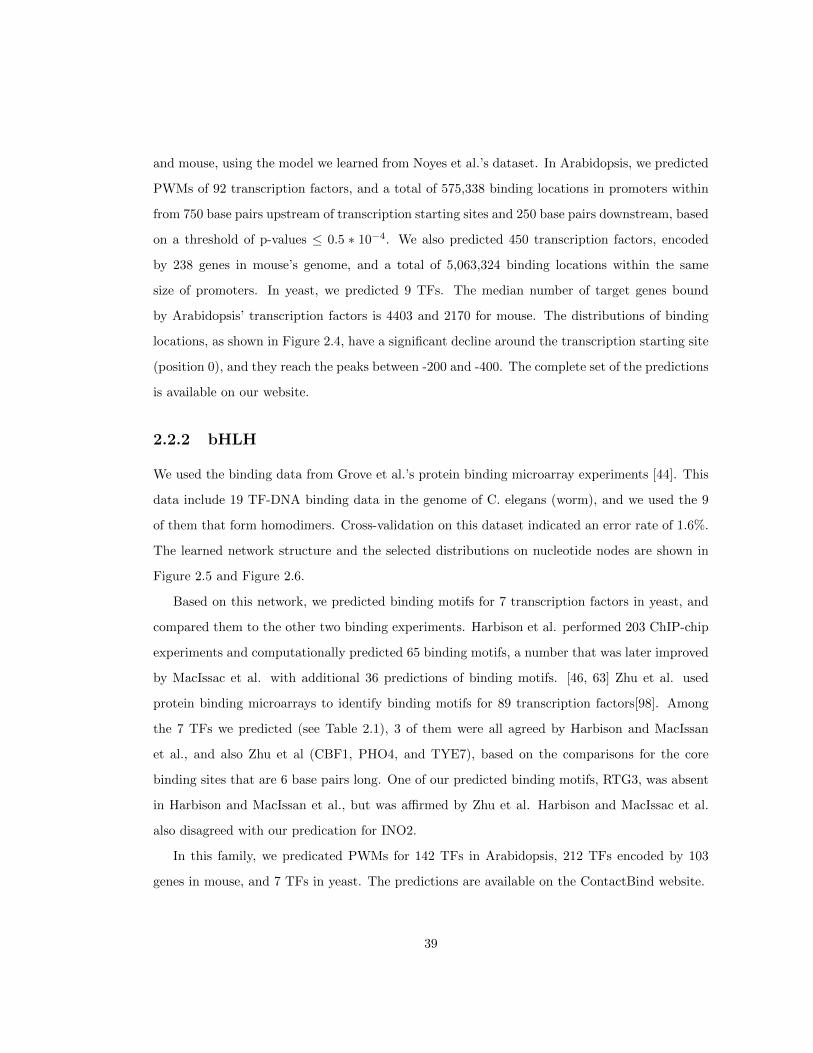
and mouse, using the model we learned from Noyes et al.’s dataset. In Arabidopsis, we predicted

PWMs of 92 transcription factors, and a total of 575,338 binding locations in promoters within

from 750 base pairs upstream of transcription starting sites and 250 base pairs downstream, based

on a threshold of p-values ≤ 0.5 ∗ 10−4. We also predicted 450 transcription factors, encoded

by 238 genes in mouse’s genome, and a total of 5,063,324 binding locations within the same

size of promoters. In yeast, we predicted 9 TFs. The median number of target genes bound

by Arabidopsis’ transcription factors is 4403 and 2170 for mouse. The distributions of binding

locations, as shown in Figure 2.4, have a significant decline around the transcription starting site

(position 0), and they reach the peaks between -200 and -400. The complete set of the predictions

is available on our website.

2.2.2 bHLH

We used the binding data from Grove et al.’s protein binding microarray experiments [44]. This

data include 19 TF-DNA binding data in the genome of C. elegans (worm), and we used the 9

of them that form homodimers. Cross-validation on this dataset indicated an error rate of 1.6%.

The learned network structure and the selected distributions on nucleotide nodes are shown in

Figure 2.5 and Figure 2.6.

Based on this network, we predicted binding motifs for 7 transcription factors in yeast, and

compared them to the other two binding experiments. Harbison et al. performed 203 ChIP-chip

experiments and computationally predicted 65 binding motifs, a number that was later improved

by MacIssac et al. with additional 36 predictions of binding motifs. [46, 63] Zhu et al. used

protein binding microarrays to identify binding motifs for 89 transcription factors[98]. Among

the 7 TFs we predicted (see Table 2.1), 3 of them were all agreed by Harbison and MacIssan

et al., and also Zhu et al (CBF1, PHO4, and TYE7), based on the comparisons for the core

binding sites that are 6 base pairs long. One of our predicted binding motifs, RTG3, was absent

in Harbison and MacIssan et al., but was affirmed by Zhu et al. Harbison and MacIssac et al.

also disagreed with our predication for INO2.

In this family, we predicated PWMs for 142 TFs in Arabidopsis, 212 TFs encoded by 103

genes in mouse, and 7 TFs in yeast. The predictions are available on the ContactBind website.

39

Binding Positions

Den

sity

0.00090

0.00095

0.00100

0.00105

0.00110

−600 −400 −200 0 200

Arabidopsis

−600 −400 −200 0 200

mouse

Figure 2.4: Distributions of predicted binding locations in the genome Arabidopsis and mouse. Pro-

moters, from 750 bp upstream of transcription starting site (TSS) to 250 downstream, were

extracted and scanned by predicted PWMs for homeodomains. Locations of binding sites

with p-values< 0.5 ∗ 10−4 were reported. Both density curves decline around TSS (the

position 0) and peaks between -200 and -400 upstream of TSS.

40

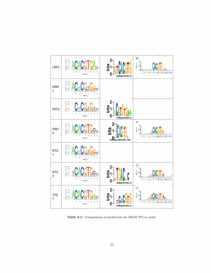
TF   Bayesian  Network   ChIP-­‐chip   Protein  Binding  Microarray  

CBF1  

     

HMS1  

 

   

INO2  

   

 

PHO4  

     

RTG1  

 

   

RTG3  

     

TYE7  

       

Table 2.1: Comparisons of predictions for bHLH TFs in yeast.

41

DNA−1 DNA1 DNA2 DNA3 DNA4DNA5 DNA6 DNA7 DNA8

AA110 AA111AA112AA113 AA114 AA115 AA116 AA117 AA119AA120 AA122 AA123 AA124

Figure 2.5: Learned Bayesian network for bHLH. The residues on the basic region of the bHLH domain

are mapped to AA110-AA114. Core binding sites in the bHLH family are about 6 base

pairs long and are positioned from DNA1 to DNA6.

2.2.3 MADS-box

We extracted 37 transcription factors and 401 binding sites from TRANSFAC [47], a cross-

species database collecting published binding sites. The error rate of our model, measured by

cross-validation as described in Section 2.4, was 11.0%. The learned network structure and

distributions, as shown in Figure 2.7 and 2.8, indicated a relatively simple network with only 3

contact points, possibly due to the currently limited availability of data.

We predicated PWMs for 108 TFs in Arabidopsis, 9 TFs that are encoded by 5 genes in

mouse, and also 4 TFs in yeast. The predictions are available on the ContactBind website.

2.2.4 The ContactBind website

Our analysis is publicly available on the ContactBind website. It provides predictions of PWMs

and their binding locations in promoters for 3 families across several species. It also includes

tools for predicting binding sites for novel transcription factors in the families we studied. Users

can also construct their own models on the website once such familial binding datasets becomes

available. The website, as shown in Figure 2.9, currently supports 1) browsing predicted PWMs,

42

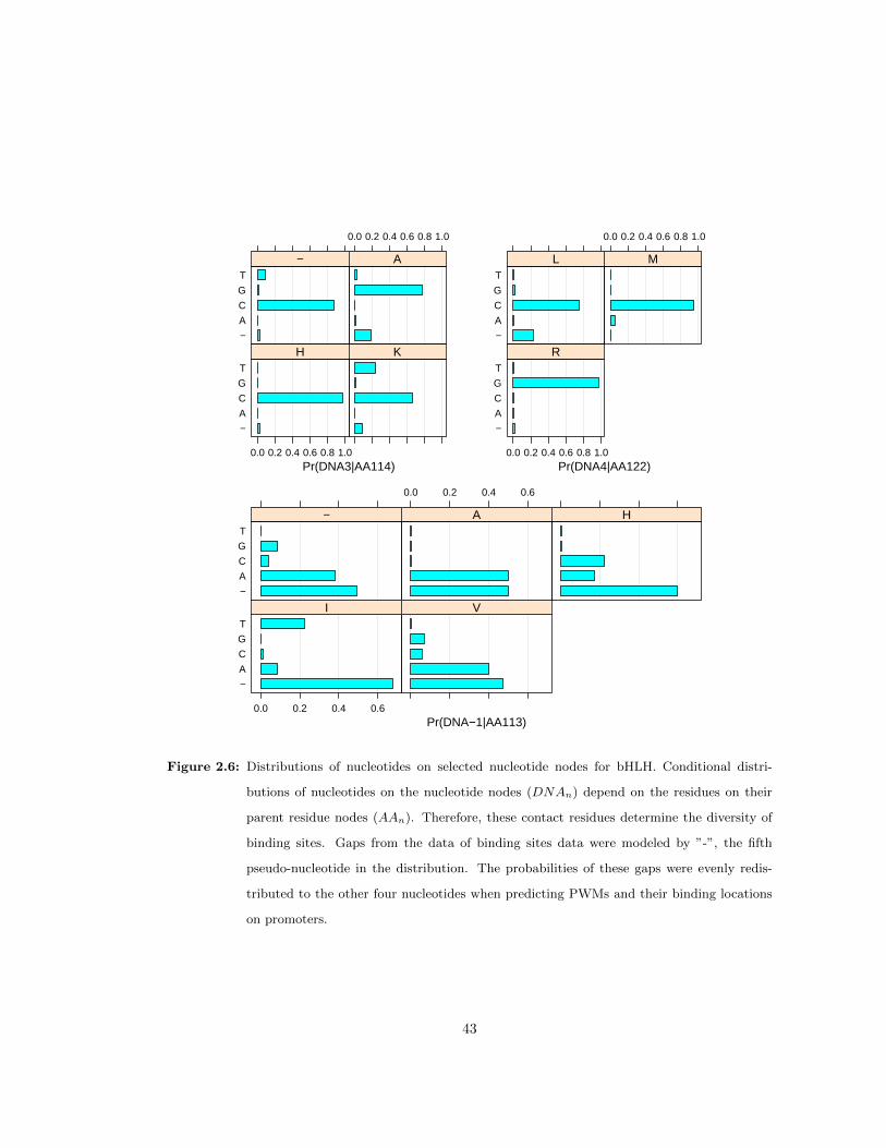
Pr(DNA−1|AA113)

−

A

C

G

T

−

0.0 0.2 0.4 0.6

A H

−

A

C

G

T

0.0 0.2 0.4 0.6

I V

Pr(DNA3|AA114)

−

A

C

G

T

−

0.0 0.2 0.4 0.6 0.8 1.0

A

−

A

C

G

T

0.0 0.2 0.4 0.6 0.8 1.0

H K

Pr(DNA4|AA122)

−

A

C

G

T

L

0.0 0.2 0.4 0.6 0.8 1.0

M

−

A

C

G

T

0.0 0.2 0.4 0.6 0.8 1.0

R

Figure 2.6: Distributions of nucleotides on selected nucleotide nodes for bHLH. Conditional distri-

butions of nucleotides on the nucleotide nodes (DNAn) depend on the residues on their

parent residue nodes (AAn). Therefore, these contact residues determine the diversity of

binding sites. Gaps from the data of binding sites data were modeled by ”-”, the fifth

pseudo-nucleotide in the distribution. The probabilities of these gaps were evenly redis-

tributed to the other four nucleotides when predicting PWMs and their binding locations

on promoters.

43

AA149 AA150 AA152 AA153 AA154 AA155 AA156 AA157 AA158 AA159 AA160 AA161 AA162

DNA1DNA2DNA3 DNA4 DNA5DNA6 DNA7DNA8 DNA9 DNA10

Figure 2.7: Learned Bayesian network for MADS-box. The residues that span part of the N-terminal

extension are mapped to AA149-AA152, while the rest residue nodes AA153-AA163 are

located on the whole contact helix. Core binding sites for the MADS-box family are 10

base pairs long and are positioned from DNA1 to DNA10.

2) browsing predicted binding locations, 3) predicting PWMs and their binding positions, given

novel protein sequences and promoter sequences, 4) learning Bayesian network for new families

and predict PWMs and their binding locations, given a pre-aligned binding dataset. The website

is hosted on http://contactbind.bio.nyu.edu.

2.2.5 Statistical dependency vs. physical interaction

Despite our original goal to model physical interactions between transcription factors and binding

sites, what we learned from the data are actually statistically dependences. In homeodomain,

our model did learn important contact residues such as AA50 and AA54, as reported previously

[50]. However, we also learned dependences where physical interactions remain unknown. There

are several possible explanations, in additional to biases in experimental data or the model itself:

the existence of physical interactions in some transcription factors that haven’t yet been crys-

tallized and examined, structure related recognitions such as DNA bending [83], or the indirect

dependences where one residue depends on the other that make contact with binding sites, yet

only the edge from the former residue to DNA was learned.

44

Pr(DNA2|AA155)

A

C

G

T

I

0.0 0.2 0.4 0.6 0.8 1.0

L

A

C

G

T

R S

A

C

G

T

0.0 0.2 0.4 0.6 0.8 1.0

T V

Pr(DNA5|AA161)

A

C

G

T

F

A

C

G

T

0.0 0.2 0.4 0.6

Y

Pr(DNA6|AA153)

A

C

G

T

D

A

C

G

T

0.0 0.2 0.4 0.6 0.8

N

Pr(DNA9|AA153)

A

C

G

T

D

A

C

G

T

0.0 0.2 0.4 0.6 0.8

N

Figure 2.8: Distributions of nucleotides on selected nucleotide nodes for MADS-box. Conditional dis-

tributions of nucleotides on the nucleotide nodes (DNAn) depend on the residues on their

parent residue nodes (AAn). Therefore, these contact residues on AA153, AA155 and

AA161 predict all of the diversity of binding sites within MADS-box.

45

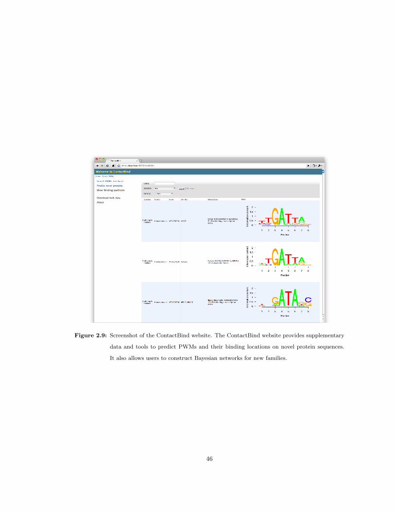
Figure 2.9: Screenshot of the ContactBind website. The ContactBind website provides supplementary

data and tools to predict PWMs and their binding locations on novel protein sequences.

It also allows users to construct Bayesian networks for new families.

46

Some counter-intuitive cases might need further crystal structure studies. For example, AA6

on MSX1 MOUSE was reported to make a nonspecific hydrogen bond with the DNA phosphate

backbone [50]. However, our model on the homeodomain family did suggest that the mutation

on this residue node changed its DNA2 binding affinity (e.g. G, H, L, R − > G, whereas A, I,

K, P, Q − > A).

Similar to biophysical models, our model has the potential to learn the reverse dependences

from the nucleotide nodes to the residue nodes. We can predict the mutations required on

novel transcription factors to change their binding affinity. In this work, we limited our scope to

predicting binding sites only, but the work also suggests the need for mutagenesis or biochemistry

analysis.

2.3 Conclusions

We proposed a novel method to model the dependences between contact residues and binding

sites, and predicted binding motifs and their locations in promoters. We made predictions for

three families of transcription factors in three species. Error rates of our method, when validated

by cross-validation, were 3.5%, 1.6%, and 16.4%, for homeodomain, bHLH, and MADS-box,

respectively. Cross-dataset validation, when learned from Noyes et at.’s fly binding data and

validated by Berger et at.’s mouse data, showed a 21.6% error rate for these cross-species pre-

dictions.

Our predictions and tools are publicly available on the ContactBind website. The website

provides tools for predicting binding motifs for novel transcription factors in the families we

studied. Users can also construct their own models on the website once such familial binding

datasets are available.

47

2.4 Materials and Methods

2.4.1 Learning Bayesian networks

The input to our model is a set of paired protein sequences of transcription factors and their

binding site sequences, where each pair is assumed to be a sample generated by the network and

each nucleotide or residue in the pair is the outcome generated by an individual graph node.

Protein and binding site sequences were pre-aligned and mapped onto the graph nodes according

to their positions within the sequences. The alignment protocols are described in detail in the

next section.

We learned both the Bayesian network structure and its model parameters: a set of probability

distributions of residues or nucleotides on the graph nodes. We employed a hill-climbing strategy

to find the network structure that maximizes its goodness-of-fit score to the input dataset. This

strategy iteratively modifies the network structure, by adding or removing a single edge, until

the score converges. Starting with the simplest network structure, a graph without any edges,

this strategy tries each possible edge from the residue nodes to the nucleotide nodes and keeps

the network structure with the best score, and then refines from this structure in the next

iteration. Model parameters, the probability distributions on the graph nodes, are estimated by

the maximum likelihood estimate after the network structured is decided.

Bayesian information criterion (BIC) was selected as our goodness-of-fit score due to its

model shrinkage capability and its among-the-best performance. Cross-validations on Noyes et

al’s homeodomain binding data indicated a 3.5% error rate (see below for the methods), while

5% with Akaike Information Criterion, 4.5% with Bayesian Dirichlet equivalent, and 3.8% with

K2 [24]. We used the bnlearn package for both the structure learning and the model parameter

fitting [85].

2.4.2 Alignment of protein and binding site sequences

In order to thread sequences onto the network nodes, protein and binding site sequences were

aligned and mapped using a variety of protocols. For aligning protein sequences, we selected

a representative crystal structure of TF-DNA binding complex for each family, and aligned the

48

protein sequences with the sequence used in the structure. Aligned subsequences located in

DNA-binding regions were extracted, and each of the residues was mapped onto a residue node.

To align binding site sequences, we devised different strategies for each family, but generally, the

steps involve using the reported familial consensuses.

We used profile hidden Markov models (HMMs) to align the input protein sequences of

transcription factors, implemented by the HMMER3 software package [31]. Pfam [35] provides

HMMs profiles for each family that were learned from curated alignments of multiple sequences

in the family. The familial profiles we used are PF00046 (homeodomain), PF00010 (bHLH)

and PF00319 (MADS-Box). The positions of the aligned protein sequences were numbered

according to the numbers used in the representative crystal structure papers, by aligning with

the anchor protein sequences in the structures. The anchor sequences we used are MSX1 MOUSE

(homeodomain) [50], MYOD1 MOUSE (bHLH) [61], and SRF HUMAN [78].

We used Noyes’s bacteria one hybrid (B1H) binding dataset for constructing the Bayesian

network for the homeodomain family. Protein sequences and binding sites were extracted from

their supplementary data. All the binding sites in the family were pre-aligned through a series of

steps including computational methods and authors’ decisions. One familial pattern of binding

sites in this family is the conservation of Ade on DNA3, which is bound by Asn on AA51. Using

Ade on DNA3 as the familial consensus, Noyes et al. constructed a master binding motif and

subsequently aligned all the binding sites onto it.

Instead of using all the 60 amino acids in homeodomain, we restricted the complexity of

learning by using only the residues on the N-terminal arm, AA2-AA8, and the third helix, AA47-

AA55. The MSX1 MOUSE structure did suggest specific contact residues, but some of them are

not consistent throughout the family. Instead of summarizing specific contact positions from

various structures, we used the whole DNA-contacting regions and relied on the goodness-of-fit

scoring function for model shrinkage.

We downloaded Grove et al.’s binding data on from UniProbe [71]. The top 40 gapped 8-mer

binding sites for each transcription factor, sorted by their enrichment scores [7, 6] were extracted

and aligned to the familial consensus, CANNTG and CANNCG. Consensuses were converted

into PWMs to score the binding sites, and only the highest-scored positions in binding sites are

extracted and mapped on to the nucleotide nodes. Protein sequences were downloaded from

49

UniProt [91]. After the alignment, the basic region, AA110-AA124, that contacts with DNA

were extracted and mapped onto the residue nodes.

For the MADS-box family, both transcription factor and binding site sequences were extracted

from TRANSFAC. Residues from AA149 to AA163 that span part of the N-terminal extension

and the whole contact helix were extracted and mapped onto the residue nodes (the helix starts

at AA153). Since binding sites reported in TRANSFAC were usually longer than the family

consensuses and located on an unspecified strand, we aligned both strand of binding sites using

their familial consensuses, CTA(A/T)4TAG and CC(A/T)6GG. Consensuses were converted into

PWMs to score the binding sites. The highest-scored subsequences with the highest scores within

the binding sites were extracted and mapped on to the nucleotide nodes.

2.4.3 Prediction of PWMs and binding locations

Probability distributions of nucleotides on nucleotide nodes in the network were converted into

columns of the PWM. For independent distributions, whose nucleotide nodes have no incoming

edges, each distribution is simply a column of the PWM where the position of the column within

the PWM is determined by the position of the node in binding sites. Some datasets might

have gaps in their binding sites and these gaps were modeled by the fifth nucleotide, ”-”, in the

distributions. The probability of the gap, if it existed, was redistributed evenly to all the other

four nucleotides within the distribution before conversion into a column.

The conditional distribution, a collection of independent distributions indexed by their dis-

crete parent residues, required look-up by the input residues on the parent residue nodes. Protein

sequences of the transcription factor, for which we predict the PWM, were aligned and mapped

to the anchor sequence, as we did when learning the network. These input residues that were

mapped on the parent residue nodes were used to locate the entry to an independent distribution

inside the conditional distribution. This independent one was converted into the column of the

PWM as usual. In some cases, however, the input residues on parent nodes might never appear

in the training set, so the corresponding entry wasn’t learned and doesn’t exist. In this case, we

picked the closest entry whose parent residues have the highest sum of the substitution scores to

the input residues. This substitution score, based on evolutionary distances among amino acids,

50

was summarized in the BLOSUM45 substitution matrix [48].

To identify potential binding locations, we scored candidate binding sites within both strands

of the promoters regions, ranging from 750 base pairs upstream of transcription starting sites to

250 base pairs downstream. The genome sequences and the locations of transcription starting

sites were obtained from several Bioconductor’s packages [42, 17, 74, 16, 75]. To calculate p-

values for these scores, we first ranked the scores of all candidate binding sites and used their

percentiles as the p-values. Candidate binding sites with p-values < 0.5 ∗ 10−4 were reported.

2.4.4 Cross-validation

We used 10-fold cross-validation to evaluate our model’s performance. The training set, a set

of pairs of TF-DNA sequences, were partitioned into 10 folds, where each fold was iteratively

withheld from the training process but used for validation on the network learned from the

other folds of the training set. In each fold, we compared the predicted binding motifs for the

transcription factors to the binding site sequences reported in the training set, by scoring each

binding site with the PWM that models the binding motif.

We scored each pair of the binding site sequence and the predicted PWM by calculating the

product of probabilities of nucleotides that appeared in the binding site, where the probabilities

of nucleotides on each position in the binding sites were retrieved from the PWM, as described in

[2]. P-values for the scores were derived from the upper percentiles of the scores in a distribution

of background scores that were generated by scoring the PWM to 10,000 random binding sites.

We used a threshold of p-values ≤ 0.01 to determine if a pair was successfully predicted, and

reported the ratio of the incorrectly predicted ones as the error rate.

2.4.5 Cross-dataset validation

A Bayesian network was constructed based on Noyes et al’s fly binding data, and was used to

predict binding motifs of mouse homeodomain TFs, where the mouse protein sequences were

downloaded from UniProt [91]. We compared our prediction to Berger et al.’s 166 mouse home-

odomain binding motifs, retrieved from UniProbe [71]. Binding motifs, both modeled by PWMs,

were compared using a similarity score that sums up Pearson correlations between distributions

51

of nucleotides on columns of the two PWMs. These two PWMs were aligned by sliding the shorter

one (in terms of the length of binding sites or the number of columns in PWMs) over the longer

one to find the alignment with the highest score. P-values of similarity scores were derived from

the upper percentiles of the scores in a background distribution of scores that were generated by

comparing the shorter PWM to a null model of 10,000 random PWMs. We used the threshold

of 0.001 in p-values to determine whether our predicted PWMs match the experimented ones.

52

Bibliography

[1] Markus Affolter, Matthew Slattery, and Richard S Mann. A lexicon for homeodomain-dna

recognition. Cell, 133(7):1133–5, Jun 2008.

[2] T L Bailey and M Gribskov. Combining evidence using p-values: application to sequence

homology searches. Bioinformatics, 14(1):48–54, 1998.

[3] Timothy L Bailey, Mikael Boden, Fabian A Buske, Martin Frith, Charles E Grant, Luca

Clementi, Jingyuan Ren, Wilfred W Li, and William S Noble. Meme suite: tools for motif

discovery and searching. Nucleic Acids Res, 37(Web Server issue):W202–8, Jul 2009.

[4] T. Barrett, D. B. Troup, S. E. Wilhite, P. Ledoux, D. Rudnev, C. Evangelista, I. F. Kim,

A. Soboleva, M. Tomashevsky, K. A. Marshall, K. H. Phillippy, P. M. Sherman, R. N. Muert-

ter, and R. Edgar. Ncbi geo: archive for high-throughput functional genomic data. Nucleic

acids research, 37:D885–D890, 2009. Sp. Iss. SI 386TT Times Cited:46 Cited References

Count:12.

[5] Michael F Berger, Gwenael Badis, Andrew R Gehrke, Shaheynoor Talukder, Anthony A

Philippakis, Lourdes Pena-Castillo, Trevis M Alleyne, Sanie Mnaimneh, Olga B Botvinnik,

Esther T Chan, Faiqua Khalid, Wen Zhang, Daniel Newburger, Savina A Jaeger, Quaid D

Morris, Martha L Bulyk, and Timothy R Hughes. Variation in homeodomain dna binding

revealed by high-resolution analysis of sequence preferences. Cell, 133(7):1266–76, Jun 2008.

[6] Michael F Berger and Martha L Bulyk. Universal protein-binding microarrays for the com-

prehensive characterization of the dna-binding specificities of transcription factors. Nat

Protoc, 4(3):393–411, 2009.

[7] Michael F Berger, Anthony A Philippakis, Aaron M Qureshi, Fangxue S He, Preston W

Estep, 3rd, and Martha L Bulyk. Compact, universal dna microarrays to comprehensively

determine transcription-factor binding site specificities. Nat Biotechnol, 24(11):1429–35, Nov

2006.

53

[8] A. Bergman and M. L. Siegal. Evolutionary capacitance as a general feature of complex

gene networks. Nature, 424(6948):549–52, 2003.

[9] K. Birnbaum, D. E. Shasha, J. Y. Wang, J. W. Jung, G. M. Lambert, D. W. Galbraith, and

P. N. Benfey. A gene expression map of the arabidopsis root. Science, 302(5652):1956–60,

2003.

[10] G. Blanc, K. Hokamp, and K. H. Wolfe. A recent polyploidy superimposed on older large-

scale duplications in the arabidopsis genome. Genome Res, 13(2):137–44, 2003.

[11] G. Blanc and K. H. Wolfe. Functional divergence of duplicated genes formed by polyploidy

during arabidopsis evolution. Plant Cell, 16(7):1679–91, 2004.

[12] G. Blanc and K. H. Wolfe. Widespread paleopolyploidy in model plant species inferred from

age distributions of duplicate genes. Plant Cell, 16(7):1667–78, 2004.

[13] N. Bouche and D. Bouchez. Arabidopsis gene knockout: phenotypes wanted. Curr Opin

Plant Biol, 4(2):111–7, 2001.

[14] S. M. Brady, D. A. Orlando, J. Y. Lee, J. Y. Wang, J. Koch, J. R. Dinneny, D. Mace,

U. Ohler, and P. N. Benfey. A high-resolution root spatiotemporal map reveals dominant

expression patterns. Science, 318(5851):801–6, 2007.

[15] G. C. Briggs, K. S. Osmont, C. Shindo, R. Sibout, and C. S. Hardtke. Unequal genetic

redundancies in arabidopsis–a neglected phenomenon? Trends Plant Sci, 11(10):492–8,

2006.

[16] Marc Carlson, Seth Falcon, Herve Pages, and Nianhua Li. org.At.tair.db: Genome wide

annotation for Arabidopsis. R package version 2.4.3.

[17] Marc Carlson, Seth Falcon, Herve Pages, and Nianhua Li. org.At.tair.db: Genome wide

annotation for Arabidopsis, 2010. R package version 2.4.3.

[18] R. Caruana and A. Niculescu-Mizil. An empirical comparison of supervised learning algo-

rithms. pages 161–168. ACM New York, NY, USA, 2006.

54

[19] S. Le Cessie and J. C. Van Houwelingen. Ridge estimators in logistic regression. Applied

Statistics, 41(1):191–201, 1992.

[20] Chih-Chung Chang and Chih-Jen Lin. Libsvm: a library for support vector machines.

software available at http://www.csie.ntu.edu.tw/ cjlin/libsvm, 2001.

[21] A. Clare, A. Karwath, H. Ougham, and R. D. King. Functional bioinformatics for arabidopsis

thaliana. Bioinformatics, 22(9):1130–6, 2006.

[22] A. Clare and R. D. King. Machine learning of functional class from phenotype data. Bioin-

formatics, 18(1):160–6, 2002.

[23] A. Clare and R. D. King. Predicting gene function in saccharomyces cerevisiae. Bioinfor-

matics, 19 Suppl 2:ii42–9, 2003.

[24] G. F. Cooper and E. Herskovits. A bayesian method for the induction of probabilistic

networks from data. Machine Learning, 9(4):309–347, 1992.

[25] C Cortes and V Vapnik. Support-vector networks. Machine Learning, 20(3):273–297, 1995.

[26] D. J. Craigon, N. James, J. Okyere, J. Higgins, J. Jotham, and S. May. Nascarrays: a

repository for microarray data generated by nasc’s transcriptomics service. Nucleic Acids

Res, 32(Database issue):D575–7, 2004. Craigon, David J James, Nick Okyere, John Higgins,

Janet Jotham, Joan May, Sean England Nucleic acids research Nucleic Acids Res. 2004 Jan

1;32(Database issue):D575-7.

[27] S. Cutler and P. McCourt. Dude, where’s my phenotype? dealing with redundancy in

signaling networks. Plant Physiology, 138(2):558–9, 2005.

[28] E. J. Dean, J. C. Davis, R. W. Davis, and D. A. Petrov. Pervasive and persistent redundancy

among duplicated genes in yeast. PLoS Genet, 4(7):e1000113, 2008.

[29] J. R. Dinneny, T. A. Long, J. Y. Wang, J. W. Jung, D. Mace, S. Pointer, C. Barron, S. M.

Brady, J. Schiefelbein, and P. N. Benfey. Cell identity mediates the response of arabidopsis

roots to abiotic stress. Science, 320(5878):942–5, 2008. Dinneny, Jose R Long, Terri A

Wang, Jean Y Jung, Jee W Mace, Daniel Pointer, Solomon Barron, Christa Brady, Siobhan

55

M Schiefelbein, John Benfey, Philip N Research Support, N.I.H., Extramural Research Sup-

port, U.S. Gov’t, Non-P.H.S. United States Science (New York, N.Y.) Science. 2008 May

16;320(5878):942-5. Epub 2008 Apr 24.

[30] P. Domingos. The role of occam’s razor in knowledge discovery. Data Mining and Knowledge

Discovery, 3(4):409–425, 1999. 261MB Times Cited:61 Cited References Count:102.

[31] S R Eddy. Profile hidden markov models. Bioinformatics, 14(9):755–63, 1998.

[32] M Elrod-Erickson, T E Benson, and C O Pabo. High-resolution structures of variant

zif268-dna complexes: implications for understanding zinc finger-dna recognition. Struc-

ture, 6(4):451–64, Apr 1998.

[33] S Falcon and R Gentleman. Using gostats to test gene lists for go term association. Bioin-

formatics, 23(2):257, 2007.

[34] J. A. Fawcett, S. Maere, and Y. Van de Peer. Plants with double genomes might have

had a better chance to survive the cretaceous-tertiary extinction event. Proceedings of the

National Academy of Sciences of the United States of America, 106(14):5737–5742, 2009.

430CX Times Cited:12 Cited References Count:54.

[35] Robert D Finn, Jaina Mistry, John Tate, Penny Coggill, Andreas Heger, Joanne E Polling-

ton, O Luke Gavin, Prasad Gunasekaran, Goran Ceric, Kristoffer Forslund, Liisa Holm, Erik

L L Sonnhammer, Sean R Eddy, and Alex Bateman. The pfam protein families database.

Nucleic Acids Res, 38(Database issue):D211–22, Jan 2010.

[36] A. Force, W. A. Cresko, F. B. Pickett, S. R. Proulx, C. Amemiya, and M. Lynch. The origin

of subfunctions and modular gene regulation. Genetics, 170(1):433–46, 2005.

[37] A. Force, M. Lynch, F. B. Pickett, A. Amores, Y. L. Yan, and J. Postlethwait. Preservation

of duplicate genes by complementary, degenerative mutations. Genetics, 151(4):1531–45,

1999.

[38] E. Frank and I. H. Witten. Generating accurate rule sets without global optimization. Proc.

15th International Conf. on Machine Learning, pages 144–151, 1998.

56

[39] TS Furey, N Cristianini, N Duffy, DW Bednarski, M Schummer, and D Haussler. Sup-

port vector machine classification and validation of cancer tissue samples using microarray

expression data. Bioinformatics, 16(10):906, 2000.

[40] W J Gehring, M Affolter, and T Burglin. Homeodomain proteins. Annual Review of Bio-

chemistry, 63(1):487–526, 1994.

[41] R Gentleman, V Carey, D Bates, B Bolstad, M Dettling, S Dudoit, B Ellis, L Gautier,

Y Ge, and J Gentry. Bioconductor: open software development for computational biology

and bioinformatics. Genome biology, 5(10):R80, 2004.

[42] Robert C Gentleman, Vincent J. Carey, Douglas M. Bates, et al. Bioconductor: Open

software development for computational biology and bioinformatics. Genome Biology, 5:R80,

2004.

[43] M. L. Gifford, A. Dean, R. A. Gutierrez, G. M. Coruzzi, and K. D. Birnbaum. Cell-specific

nitrogen responses mediate developmental plasticity. Proc Natl Acad Sci U S A, 105(2):803–

8, 2008.

[44] Christian A Grove, Federico De Masi, M Inmaculada Barrasa, Daniel E Newburger, Mark J

Alkema, Martha L Bulyk, and Albertha J M Walhout. A multiparameter network reveals

extensive divergence between c. elegans bhlh transcription factors. Cell, 138(2):314–27, Jul

2009.

[45] M. A. Hall and L. A. Smith. Feature subset selection: a correlation based filter approach.

pages 855–858, 1997. Proceedings of the Fourth International Conference on Neural Infor-

mation Processing and Intelligent Information Systems.

[46] Christopher T Harbison, D Benjamin Gordon, Tong Ihn Lee, Nicola J Rinaldi, Kenzie D

Macisaac, Timothy W Danford, Nancy M Hannett, Jean-Bosco Tagne, David B Reynolds,

Jane Yoo, Ezra G Jennings, Julia Zeitlinger, Dmitry K Pokholok, Manolis Kellis, P Alex

Rolfe, Ken T Takusagawa, Eric S Lander, David K Gifford, Ernest Fraenkel, and Richard A

Young. Transcriptional regulatory code of a eukaryotic genome. Nature, 431(7004):99–104,

Sep 2004.

57

[47] T Heinemeyer, E Wingender, I Reuter, H Hermjakob, A E Kel, O V Kel, E V Ignatieva,

E A Ananko, O A Podkolodnaya, F A Kolpakov, N L Podkolodny, and N A Kolchanov.

Databases on transcriptional regulation: Transfac, trrd and compel. Nucleic Acids Res,

26(1):362–7, Jan 1998.

[48] S Henikoff and J G Henikoff. Amino acid substitution matrices from protein blocks. Proc

Natl Acad Sci U S A, 89(22):10915–9, Nov 1992.

[49] M. E. Hillenmeyer, E. Fung, J. Wildenhain, S. E. Pierce, S. Hoon, W. Lee, M. Proctor,

R. P. St Onge, M. Tyers, D. Koller, R. B. Altman, R. W. Davis, C. Nislow, and G. Giaever.

The chemical genomic portrait of yeast: uncovering a phenotype for all genes. Science,

320(5874):362–5, 2008.

[50] S Hovde, C Abate-Shen, and J H Geiger. Crystal structure of the msx-1 homeodomain/dna

complex. Biochemistry, 40(40):12013–21, Oct 2001.

[51] J D Hughes, P W Estep, S Tavazoie, and G M Church. Computational identification of cis-

regulatory elements associated with groups of functionally related genes in saccharomyces

cerevisiae. J Mol Biol, 296(5):1205–14, Mar 2000.

[52] G. H. John and P. Langley. Estimating continuous distributions in bayesian classifiers.

Proceedings of the Eleventh Conference on Uncertainty in Artificial Intelligence, pages 338–

345, 1995.

[53] Susan Jones. An overview of the basic helix-loop-helix proteins. Genome Biol, 5(6):226,

2004.

[54] Tommy Kaplan, Nir Friedman, and Hanah Margalit. Ab initio prediction of transcription

factor targets using structural knowledge. PLoS Comput Biol, 1(1):e1, Jun 2005.

[55] O. D. King, J. C. Lee, A. M. Dudley, D. M. Janse, G. M. Church, and F. P. Roth. Predicting

phenotype from patterns of annotation. Bioinformatics, 19 Suppl 1:i183–9, 2003.

[56] M. A. Larkin, G. Blackshields, N. P. Brown, R. Chenna, P. A. McGettigan, H. McWilliam,

F. Valentin, I. M. Wallace, A. Wilm, R. Lopez, J. D. Thompson, T. J. Gibson, and D. G.

58

Higgins. Clustal w and clustal x version 2.0. Bioinformatics, 23(21):2947–8, 2007. Larkin,

M A Blackshields, G Brown, N P Chenna, R McGettigan, P A McWilliam, H Valentin,

F Wallace, I M Wilm, A Lopez, R Thompson, J D Gibson, T J Higgins, D G Research

Support, Non-U.S. Gov’t England Bioinformatics (Oxford, England) Bioinformatics. 2007

Nov 1;23(21):2947-8. Epub 2007 Sep 10.

[57] J. Y. Lee, J. Colinas, J. Y. Wang, D. Mace, U. Ohler, and P. N. Benfey. Transcriptional and

posttranscriptional regulation of transcription factor expression in arabidopsis roots. Proc

Natl Acad Sci U S A, 103(15):6055–60, 2006.

[58] S. Li, C. M. Armstrong, N. Bertin, H. Ge, S. Milstein, M. Boxem, P. O. Vidalain, J. D.

Han, A. Chesneau, T. Hao, D. S. Goldberg, N. Li, M. Martinez, J. F. Rual, P. Lamesch,

L. Xu, M. Tewari, S. L. Wong, L. V. Zhang, G. F. Berriz, L. Jacotot, P. Vaglio, J. Reboul,

T. Hirozane-Kishikawa, Q. Li, H. W. Gabel, A. Elewa, B. Baumgartner, D. J. Rose, H. Yu,

S. Bosak, R. Sequerra, A. Fraser, S. E. Mango, W. M. Saxton, S. Strome, S. Van Den Heuvel,

F. Piano, J. Vandenhaute, C. Sardet, M. Gerstein, L. Doucette-Stamm, K. C. Gunsalus,

J. W. Harper, M. E. Cusick, F. P. Roth, D. E. Hill, and M. Vidal. A map of the interactome

network of the metazoan c. elegans. Science, 303(5657):540–3, 2004.

[59] R. Liu, A. M. Ferrenberg, L. U. Gilliland, R. B. Meagher, and M. A. Asmussen. Detection

of deleterious genotypes in multigenerational studies. iii. estimation of selection components

in highly selfing populations. Genet Res, 82(1):41–53, 2003.

[60] M. Lynch and A. Force. The probability of duplicate gene preservation by subfunctionaliza-

tion. Genetics, 154(1):459–73, 2000.

[61] P C Ma, M A Rould, H Weintraub, and C O Pabo. Crystal structure of myod bhlh domain-

dna complex: perspectives on dna recognition and implications for transcriptional activation.

Cell, 77(3):451–9, May 1994.

[62] T. MacCarthy and A. Bergman. The limits of subfunctionalization. BMC Evol Biol, 7:213,

2007.

59

[63] Kenzie D MacIsaac, Ting Wang, D Benjamin Gordon, David K Gifford, Gary D Stormo,

and Ernest Fraenkel. An improved map of conserved regulatory sites for saccharomyces

cerevisiae. BMC Bioinformatics, 7:113, 2006.

[64] M E Massari and C Murre. Helix-loop-helix proteins: regulators of transcription in eucary-

otic organisms. Mol Cell Biol, 20(2):429–40, Jan 2000.

[65] Francine Messenguy and Evelyne Dubois. Role of mads box proteins and their cofactors in

combinatorial control of gene expression and cell development. Gene, 316:1–21, Oct 2003.

[66] Y Mo, W Ho, K Johnston, and R Marmorstein. Crystal structure of a ternary sap-1/srf/c-fos

sre dna complex. J Mol Biol, 314(3):495–506, Nov 2001.

[67] Alexandre V Morozov, James J Havranek, David Baker, and Eric D Siggia. Protein-dna

binding specificity predictions with structural models. Nucleic Acids Res, 33(18):5781–98,

2005.

[68] Alexandre V Morozov and Eric D Siggia. Connecting protein structure with predictions of

regulatory sites. Proc Natl Acad Sci U S A, 104(17):7068–7073, Apr 2007.

[69] T. Nawy, J. Y. Lee, J. Colinas, J. Y. Wang, S. C. Thongrod, J. E. Malamy, K. Birnbaum,

and P. N. Benfey. Transcriptional profile of the arabidopsis root quiescent center. Plant

Cell, 17(7):1908–25, 2005.

[70] V. Neduva and R. B. Russell. Linear motifs: evolutionary interaction switches. FEBS Lett,

579(15):3342–5, 2005. Neduva, Victor Russell, Robert B Review Netherlands FEBS letters

FEBS Lett. 2005 Jun 13;579(15):3342-5. Epub 2005 Apr 18.

[71] Daniel E Newburger and Martha L Bulyk. Uniprobe: an online database of protein binding

microarray data on protein-dna interactions. Nucleic Acids Res, 37(Database issue):D77–82,

Jan 2009.

[72] M. A. Nowak, M. C. Boerlijst, J. Cooke, and J. M. Smith. Evolution of genetic redundancy.

Nature, 388(6638):167–71, 1997.

60

[73] Marcus B Noyes, Ryan G Christensen, Atsuya Wakabayashi, Gary D Stormo, Michael H

Brodsky, and Scot A Wolfe. Analysis of homeodomain specificities allows the family-wide

prediction of preferred recognition sites. Cell, 133(7):1277–89, Jun 2008.

[74] H. Pages. BSgenome.Athaliana.TAIR.04232008: Arabidopsis thaliana full genome (TAIR

version from April 23, 2008), 2008. R package version 1.3.16.

[75] H. Pages. BSgenome.Mmusculus.UCSC.mm9: Mus musculus (Mouse) full genome (UCSC

version mm9), 2010. R package version 1.3.16.

[76] N P Pavletich and C O Pabo. Zinc finger-dna recognition: crystal structure of a zif268-dna

complex at 2.1 a. Science, 252(5007):809–17, May 1991.

[77] Dana Pe’er. Bayesian network analysis of signaling networks: a primer. Sci STKE,

2005(281):pl4, Apr 2005.

[78] L Pellegrini, S Tan, and T J Richmond. Structure of serum response factor core bound to

dna. Nature, 376(6540):490–8, Aug 1995.

[79] JC Platt. Probabilistic outputs for support vector machines and comparisons to regularized

likelihood methods. Advances in large margin classifiers, 1999.

[80] J. R. Quinlan. Simplifying decision trees, 1986.

[81] J. R. Quinlan. C4. 5: Programs for Machine Learning. Morgan Kaufmann, 1993.

[82] SY Rhee, W Beavis, TZ Berardini, G Chen, D Dixon, A Doyle, M Garcia-Hernandez,

E Huala, G Lander, and M Montoya. The arabidopsis information resource (tair): a model

organism database providing a centralized, curated gateway to arabidopsis biology, research

materials and community. Nucleic acids research, 31(1):224, 2003.

[83] Remo Rohs, Sean M West, Alona Sosinsky, Peng Liu, Richard S Mann, and Barry Honig.

The role of dna shape in protein-dna recognition. Nature, 461(7268):1248–53, Oct 2009.

[84] M. Schmid, T. S. Davison, S. R. Henz, U. J. Pape, M. Demar, M. Vingron, B. Scholkopf,

D. Weigel, and J. U. Lohmann. A gene expression map of arabidopsis thaliana develop-

ment. Nat Genet, 37(5):501–6, 2005. Schmid, Markus Davison, Timothy S Henz, Stefan R

61

Pape, Utz J Demar, Monika Vingron, Martin Scholkopf, Bernhard Weigel, Detlef Lohmann,

Jan U Research Support, Non-U.S. Gov’t United States Nature genetics Nat Genet. 2005

May;37(5):501-6. Epub 2005 Apr 3.

[85] Marco Scutari. bnlearn: Bayesian network structure learning, 2010. R package version 2.1.

[86] A. K. Seewald. How to make stacking better and faster while also taking care of an unknown

weakness. Proceedings of the Nineteenth International Conference on Machine Learning table

of contents, pages 554–561, 2002.

[87] Christiana Spyrou, Rory Stark, Andy G Lynch, and Simon Tavare. Bayespeak: Bayesian

analysis of chip-seq data. BMC Bioinformatics, 10:299, 2009.

[88] A. L. Tarca, V. J. Carey, X. W. Chen, R. Romero, and S. Draghici. Machine learning and

its applications to biology. PLoS Comput Biol, 3(6):e116, 2007.

[89] M. Tasan, W. Tian, D. P. Hill, F. D. Gibbons, J. A. Blake, and F. P. Roth. An en masse

phenotype and function prediction system for mus musculus. Genome Biol, 9 Suppl 1:S8,

2008.

[90] D. Tautz. A genetic uncertainty problem. Trends Genet, 16(11):475–7, 2000.

[91] UniProt Consortium. The universal protein resource (uniprot) in 2010. Nucleic Acids Res,

38(Database issue):D142–8, Jan 2010.

[92] Y. Van de Peer, J. A. Fawcett, S. Proost, L. Sterck, and K. Vandepoele. The flowering

world: a tale of duplications. Trends in Plant Science, 14(12):680–688, 2009. 533WI Times

Cited:2 Cited References Count:58.

[93] A. Wagner. Redundant gene functions and natural selection. Journal of Evolutionary Biol-

ogy, 12:1–16, 1999.

[94] G. P. Wagner and V. J. Lynch. The gene regulatory logic of transcription factor evolu-

tion. Trends in Ecology and Evolution, 23(7):377–385, 2008. 325VW Times Cited:13 Cited

References Count:63.

62

[95] Ian H. Witten and Eibe Frank. Data Mining: Practical machine learning tools and tech-

niques, 2nd Edition. Morgan Kaufmann, San Francisco, 2005.

[96] Z. Yang. Paml: a program package for phylogenetic analysis by maximum likelihood. Comput

Appl Biosci, 13(5):555–6, 1997.

[97] E. T. Young, J. S. Sloan, and K. Van Riper. Trinucleotide repeats are clustered in regulatory

genes in saccharomyces cerevisiae. Genetics, 154(3):1053–68, 2000. Young, E T Sloan, J S

Van Riper, K GM26079/GM/NIGMS NIH HHS/United States R29GM54043/GM/NIGMS

NIH HHS/United States Research Support, U.S. Gov’t, P.H.S. United states Genetics Ge-

netics. 2000 Mar;154(3):1053-68.

[98] Cong Zhu, Kelsey J R P Byers, Rachel Patton McCord, Zhenwei Shi, Michael F Berger,

Daniel E Newburger, Katrina Saulrieta, Zachary Smith, Mita V Shah, Mathangi Radhakr-

ishnan, Anthony A Philippakis, Yanhui Hu, Federico De Masi, Marcin Pacek, Andreas Rolfs,

Tal Murthy, Joshua Labaer, and Martha L Bulyk. High-resolution dna-binding specificity

analysis of yeast transcription factors. Genome Res, 19(4):556–66, Apr 2009.

63