arX

iv:1

609.

0573

7v2

[con

d-m

at.m

trl-s

ci]

19 D

ec 2

016

Machine-learned approximations to DensityFunctional Theory HamiltoniansGanesh Hegde1,* and R. Chris Bowen1

1Advanced Logic Lab, Samsung Semiconductor Inc., Austin, TX 78754, USA* ganesh.h@ssi.samsung.com

ABSTRACT

Large scale Density Functional Theory (DFT) based electronic structure calculations are highly time consuming and scalepoorly with system size. While semi-empirical approximations to DFT result in a reduction in computational time versus abinitio DFT, creating such approximations involves significant manual intervention and is highly inefficient for high-throughputelectronic structure screening calculations. In this letter, we propose the use of machine-learning for prediction of DFT Hamil-tonians. Using suitable representations of atomic neighborhoods and Kernel Ridge Regression, we show that an accurateand transferable prediction of DFT Hamiltonians for a variety of material environments can be achieved. Electronic structureproperties such as ballistic transmission and band structure computed using predicted Hamiltonians compare accurately withtheir DFT counterparts. The method is independent of the specifics of the DFT basis or material system used and can easilybe automated and scaled for predicting Hamiltonians of any material system of interest.

Introduction

Density Functional Theory (DFT) based electronic structure calculations are a cornerstone of modern computational materialscience. Despite their popularity and usefulness, DFT methods scale rather poorly with system size. Even the fastest DFTtechniques, such as the so-called O(N) approaches based on Local Orbitals spend most of their time in forming the Hamiltonianand solving self-consistently for the ground state electron eigenstates1. Consequently, while it scales well for small systemssuch as crystalline solids with small unit cells, scaling the computation of DFT electronic structure for large nanostructureswith limited periodicity becomes a challenging task.

Semi-empirical Tight Binding (TB) approximations to DFT perform rather admirably in this regard, reducing the timecomplexity in forming Hamiltonians by treating Hamiltonian elements as parameters fitted to desired physical properties suchas effective mass, band gaps and so on. Typically, TB techniques also simplify the DFT Hamiltonian to near-neighbor (NN)interactions between atoms. This results in extremely sparse Hamiltonians that can be diagonalized very efficiently. Severalflavors of these approximations exist, generally optimizedto meet the needs of the problem at hand2.

While TB calculations have proved immensely useful in modeling the electronic structures of semiconductor and metallicnanostructures, some fundamental problems persist in their use as DFT Hamiltonian approximations. Firstly, while TB Hamil-tonians are computationally efficient to solve for, what is often unaccounted for is the time required to create an accurate,physically transparent and transferable TB model for a material system. In our own experience3,4, developing meaningful,physical TB parameter sets has taken time ranging from a few weeks to a few years. Secondly, developing truly transferable,physically valid TB models applicable across materials, geometries and boundary conditions is challenging, owing to physicaldifferences in systems.

There are a variety of reasons for the aforementioned shortcomings. One, it is often the case that a physically transparentmodel created for a particular material type (say semiconductors with short range, covalent bonding) does not generalize toother material systems (for instance, metals). Secondly, significant portions of the TB parameter-set creation process involvemanual intervention. From the functional form of the model used to fit Hamiltonian elements to the choice and tuning of thefitting process, the TB parameterization process often resembles art than an exact science.

This is clearly an undesirable state of affairs, especiallyin time-sensitive industrial applications where a number of materialsystems, geometries and boundary conditions need to be evaluated rapidly to test for suitability for an application. Toaddressthese issues, we propose a Machine Learning (ML) based method to predict DFT Hamiltonians. In contrast to existing semi-empirical approximations to DFT, our method does not fit parametric models to DFT Hamiltonians or derived electronicstructure quantities such as effective masses and band gaps. We instead map atomic environments to real-space Hamiltonianpredictions using non-parametric interpolation-based machine learning techniques such as Kernel Ridge Regression (KRR)5.The time-consuming direct computation of Hamiltonian integrals and ground state eigenstates in DFT is completely bypassed

1

in favor of simple matrix multiplication reducing computational cost considerably. Through rigorous criteria for selection ofalgorithm hyper-parameters, the method can be automated and transferability to new material systems can be controlled. Themethod is independent of the specifics of the material systemand depends only on the reference DFT calculations.

The paper is organized as follows. The methods section describes how the problem of predicting DFT Hamiltonians canbe mapped on to a ML framework. The results section shows the application of the method proposed in this work to twomaterial systems - a arbitrarily strained Cu system and a arbitrarily strained C (diamond) system. The Cu case study assessesthe applicability of the present technique to a relatively simple Cu-DFT system consisting only of rotation invariants-orbitalscentered on Cu atoms, while the C case study extends the technique to more realistic systems involvings andp orbitals andtheir interactions. A comparison of the advantages and limitations of the method to existing semi-empirical approximationsto DFT is included in the discussion section.

MethodsIn recent times, several advances have been made in applyinga variety of machine learning techniques to computational ma-terial science. These include (but are not limited to) the mapping of spatial atomic data to predict total energies6–8, predictionof DFT functionals9 and direct computation of electronic properties10 through machine learning. We are, however, unawareof any attempt to apply ML to the problem of DFT Hamiltonian prediction.

Applying ML to any problem presupposes the existence of dataand a unknown, non-trivial map from inputs to outputs.In supervised ML, the dataset consists of inputs/variables(henceforth referred to as ’features’) and the challenge isto find amap from features to pre-labeled/desired/reference outputs (targets). In our case, the dataset consists of inputs in the form ofsets of atomic positions while the targets consist of DFT Hamiltonian elements between orbitals centered on individualatoms.The reference data is obtained by time consuming self-consistent DFT calculations, but the aim is that once a map is obtainedfrom input to reference data, the map is sufficiently accurate and transferable to cases not explicitly included in the dataset.

Real-space DFT Hamiltonians consist of intra-atomic (between orbitals situated on the same atom) and inter-atomic (be-tween orbitals situated on different atoms) matrix elements. Most real-space DFT codes allow direct access to these elementsupon the convergence of a ground state DFT calculation. In case of plane-wave DFT codes, a projection of plane-wave basedHamiltonian can be made on to a real space basis. The rest of this paper assumes a real-space Hamiltonian. These real-spaceDFT Hamiltonian matrix elements then constitute our reference data.

Broadly speaking, intra-atomic and inter-atomic (real-space) DFT Hamiltonian elements depend on

1. The position and charges of the interacting atoms.

2. The positions and charges of atoms that are in the neighborhood of interacting atoms.

3. The basis functions (orbitals) centered on each atom.

1) and 2) above define a 3D-radially and angularly varying potential (upon DFT calculation convergence) that is highly non-trivial for the simplest of systems that go beyond a single atom. Factor 3) above is usually fully knowna priori. From thisenumeration, one can surmise that obtaining useful features required for ML requires a faithful representation of the positionsand charges of interacting atoms and their atomic neighborhood.

A possible starting point in forming features for ML is the collection of atomic positions and charges (atomic numbers).However, operations such as rotation, translation and permutation of atom numbers in an atomic dataset change their positionsand their relative ordering completely. In general, Hamiltonian elements are are invariant to translation and permutation, butchange upon a rotation reference frame (higher spherical harmonics are not rotation invariant). It is therefore important thatthe features formed reflect these properties. The atomic positions and charges must therefore be transformed to reflect theinteractions between orbitals and the atomic environment responsible in forming DFT Hamiltonian interactions.

Seminal work published in the past 10 years has realized the difficult task of invariant representation of atomic neighbor-hoods possible to the point where these approaches can readily be used in ML for a variety of computational material scienceapplications. These include the Bispectrum formalism of Bartok et al.6, the Coulomb Matrix formalism (see for instance,Rupp et al.7 and Montavon et al.11), the Symmetry Function formalism of Behler et al.8, the Partial Radial Distribution Func-tion (PRDF) formalism of Schutt et al.10, the Bag-of-Bonds (BoB) formalism of Hansen et al.12 and the Fourier Series of RDFformalism of von Lilienfeld et al.13, to name a few. In this work, we have used the bispectrum formalism of Bartok et al. torepresent the neighborhood of an atom. In this formalism, the 3D radial and angular environment of each atom is convertedinto vector of bispectrum components of the local neighbor density projected on to a basis of hyperspherical harmonics in fourdimensions. While a detailed discussion of the the formalism is beyond the scope of this work, we refer the interested readerto the literature on the topic6,14–16.

For the purpose of this work, it suffices to understand the bispectrum as a unique, vectorized representation of an atomslocal environment, so that it can be used as a basis for creating features suitable for machine learning. Figure1 is a simple

2/13

example of how the bispectrum distinguishes between different strained environments that a Face Centered Cubic (FCC) Cuatom is exposed to. The various components of the bispectrumvector can reflect subtle variations in neighbor environment,creating a unique map between features and Hamiltonian elements. Our choice of bispectrum is motivated by its rotation,translation and permutation invariant representation of theatomic environmentin a convenient vectorized form, with an abilityto tune the dimensionality of the bispectrum vector by changing the number of angular momentum channels. We hasten to addthat it should not be construed as distinctly advantageous by the reader and alternate representations of the atoms environmentthat share these features may be considered in place of the bispectrum without affecting the applicability of the present method.

2 4 6 8 10 12 14100

150

200

250

300

350

Bis

pe

ctru

m C

oe

ffic

ien

ts

Coefficient ID in Bispectrum Vector

Bulk Unstrained FCC Cu10% Hydrostatically strained FCC Cu10% Uniaxially [110] strained FCC Cu

Figure 1. Bispectrum measure for a Cu atom in 3 different FCC environments - bulk unstrained, 10% hydrostatic strain and10% uniaxial strain along [100]. The Bispectrum is a unique measure for the atom in the different environments and istherefore an excellent candidate for the creation of ML features from atomic spatial data.

s-orbitals and their interactions with other s-orbitals arerotation, translation and permutation invariant. For the Cu-casestudy where a singles-orbital centered on Cu atoms forms the basis set, our input features can then be simply formed fromthe bispectra of the atoms taking part in the interaction without explicit information about the reference frame or its rotation.For intra-atomic elements in the Cu-case study, the featurevector we use is simply the bispectrum of the respective atoms.For inter-atomic Hamiltonian elements in this case study, acandidate feature vector is the bispectrum of the two atoms takingpart in the interaction. Since 3D periodic material systemscontain an infinite number of atoms having the same neighborhood,we divide the bispectra of the two atoms taking part in the Hamiltonian interaction by their inter-atomic distance and appendthe interatomic distance to form the feature vector. We found that adding some measure of the interatomic distance explicitlyin the feature vector in addition to its implicit inclusion by (modifying the bispectrum) systematically improved predictiveperformance of our method. For instance we found that the RMSE of the inter-atomic interactions reduced by approximately2 meV with the inclusion of interatomic distance. We note, however, that we did not systematically investigate the performanceof a distance metric being explicitly included in the feature vector versus, say, inverse distance or other powers of interatomicdistance. Figure2 in the methods section shows the feature formation process for the Cu-case study in greater detail.

For the C (diamond) - case study, the simplest DFT basis set that captures electronic interactions accurately is one com-prised of a singlesorbital and 4p orbitals. While interactions betweensorbitals are rotation invariant as mentioned previously,interactions between dissimilarsandp orbitals and between dissimilarp orbitals on different atoms in general are not rotationinvariant. In addition to capturing the atomic environment, which may yet be invariant to rotations, one therefore needs to cap-ture angular information as well. For interatomic interactions, the direction cosines (l , m, n) of the bond vector (with respect tothe Cartesian axes/laboratory reference frame) between two atoms taking part in the Hamiltonian interaction were appendedto the feature vector used in the Cu-case study. Introduction of this angular information simply captures the necessaryangularinformation for interatomic elements.

The orbitals involved in intra-atomic interactions belongto the same atom, while the potential contribution to the Hamil-tonian element is from this atom and other neighboring atoms. Rotation of the reference frame or addition of atoms in theneighborhood leaves the relative angular information of the orbitals situated on the same atom unchanged i.e. still zero. Theangular information of the neighborhood, however, changesand with this rotation, the off-diagonal intra-atomic Hamiltonianelements change as well. Unlike inter-atomic interactions, however, we cannot solve this problem by simply appending neigh-bor direction cosines, since the interaction captured is between two orbitals on the same atom. This is addressed by appealingto the physics of the problem at hand. The neighbors that exert the most influence on the intra-atomic interaction are the

3/13

nearest neighbors. We therefore sum the direction cosines with respect to each Cartesian axis from each neighbor and appendthis to the bispectrum. For instance, a C atom in diamond-like configurations has 4 nearest neighbors, with direction cosinesl1, l2, l3 andl4 with respect to thex Cartesian axis. For unstrained diamond, the sum of these direction cosines is zero as is thesum of direction cosines with respect toy andz axes. This captures very well the actual DFT calculation forthe intra-atomicblock in diamond, where off-diagonal intra-atomic interactions are zero. When symmetry is broken by straining uni-axiallyfor instance, the sum of direction cosines becomes non-zero. This is reflected in the corresponding Hamiltonian where theoff-diagonal intra-atomic elements become non-zero. Thisscheme outlined above is one among a number of such schemesthat can be devised to incorporate angular interactions.

In the Slater-Koster scheme used in classical Tight-Binding17, introducing angular information in the form of directioncosines can be shown to represent the angular part of all inter-atomic Hamiltonian interactions, while canonical interatomicinteractions between orbitals -Vssσ ,Vspσ ,Vppπ ,Vppσ - can be obtained by aligning the bond-axis to the laboratory/Cartesianz-axis reference. Generally speaking, however, interatomic interactions go beyond the simple-two center scheme and theSlater Koster scheme applied fails to account for more complicated ’three-center’ interactions. This is true for intra-atomicinteractions as well, where one needs to go beyond the two-center approximation to capture non-zero off-diagonal intra-atomicHamiltonian elements. Since the aim in machine learning is typically to let the data ’find’ a reliable map upon supplyingfeatures sufficient to represent the outputs meaningfully,we have simply chosen to incorporate angular information intheform of direction cosines and their sums instead of imposinga model on the underlying interactions.

Having formed the features thus, the non-linear map from thefeatures to the Hamiltonian elements can be learned using aML technique called Kernel Ridge Regression (KRR). In KRR, the predicted output for a given feature vector is expressed asa combination of similarity measures between the feature vector (for which an output is to be predicted) and all other featurevectors in the dataset. Using the notation from Rupp18, for a feature vector ˜x, the predicted outputf (x) is given as

f (x) =n

∑i=1

αik(xi , x) (1)

Here,n is the number of training examples,k(xi , x) is the kernel measure between feature vectorsxi andx andαi is thecorresponding weight in the sum. The kernel measurek(xi , x) allows a comparison of similarity (or conversely, distance)between feature vectors5. We use a Gaussian kernel defined as follows

k(xi , x) = exp(−γ‖xi − x‖22) (2)

γ is an algorithm hyper-parameter that decides the extent (infeature space) to which the kernel operates. The second termin the exponent is the squared 2-norm of the difference vector between the two feature vectorsxi andx. The similarity kernelreturns a value of 1 when the feature vectors are identical, indicating maximum similarity. By changing the value ofγ onecan tune the extent to which the kernel returns similarity values. Forγ values close to zero, only those feature vectors that areclosely matched will return a similarity measure approaching 1, whereas feature vectors that are dissimilar will return valuesapproaching zero. For larger values ofγ, a finite similarity value is returned by the kernel for feature vectors that are unequal.

Equation1 above thus interpolates between existing feature vectors in the dataset and predicts a value based on thesimilarity of the candidate feature vector to those in the dataset. The weightsα are learned by computing the similaritymeasure between all feature vectors in the training dataset.

α = (K+λ I)−1y (3)

where the kernel matrixK is obtained by computing similarity measures using equation 2 between each feature vector in thetraining dataset,y is the vector of training reference data.λ is a regularization hyper-parameter that controls the smoothnessof the interpolator and prevents over-fitting.I is the identity matrix.

Equations1, 2 and3 together constitute the equations defining the KRR learningalgorithm. Given a training datasetX(with n feature vectorsxi and i from 1 throughn) andy (with reference outputsyi for each feature vector in the training dataset),these equations can be used to train the set of weightsα, obtain a similarity measureK for the dataset, and predict the outputvalue for a candidate feature vector ˜x for a given value of the algorithm hyper-parametersλ andγ.

Having shown how a DFT Hamiltonian problem can be mapped on toa machine learning problem, we now summarizethe requirements from a procedural perspective. First,n reference self-consistent DFT calculations on the material system ofinterest are performed. For each DFT calculation, DFT Hamiltonian elements are extracted to form the reference outputsy.For each reference outputyi , a feature vectorxi is extracted by converting the atomic positions, charges and neighborhoodsof the atoms involved in the formation of matrix elementsyi to a corresponding invariant bispectrum measure using the

4/13

Figure 2. Schematic representation of the reference dataset creation process for the Cu-case study. First the atomic structuredata in the form of atom types, charges and positions are converted to corresponding bispectra. The bispectra of differentatoms are then combined to form features for learning. For intra-atomic Hamlitonian elements (E), the bispectra of individualatoms constitute the feature vector. For inter-atomic Hamiltonian elements (V), the bispectra are divided by the inter-atomicdistances (R) to form the feature vector. The feature vectors along with their corresponding reference output data constitutethe reference dataset.

5/13

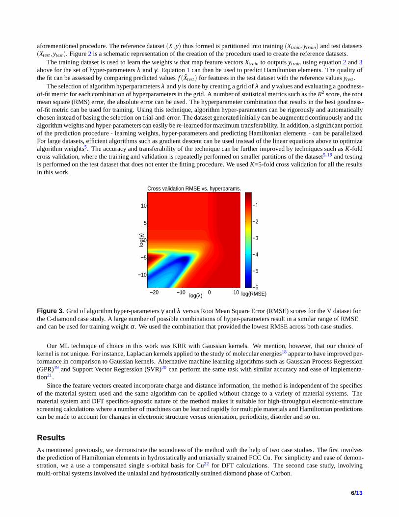
aforementioned procedure. The reference dataset(X,y) thus formed is partitioned into training(Xtrain,ytrain) and test datasets(Xtest,ytest). Figure2 is a schematic representation of the creation of the procedure used to create the reference datasets.

The training dataset is used to learn the weightsw that map feature vectorsXtrain to outputsytrain using equation2 and3above for the set of hyper-parametersλ andγ. Equation1 can then be used to predict Hamiltonian elements. The quality ofthe fit can be assessed by comparing predicted valuesf (Xtest) for features in the test dataset with the reference valuesytest.

The selection of algorithm hyperparametersλ andγ is done by creating a grid ofλ andγ values and evaluating a goodness-of-fit metric for each combination of hyperparameters in thegrid. A number of statistical metrics such as theR2 score, the rootmean square (RMS) error, the absolute error can be used. The hyperparameter combination that results in the best goodness-of-fit metric can be used for training. Using this technique,algorithm hyper-parameters can be rigorously and automaticallychosen instead of basing the selection on trial-and-error.The dataset generated initially can be augmented continuously and thealgorithm weights and hyper-parameters can easily be re-learned for maximum transferability. In addition, a significant portionof the prediction procedure - learning weights, hyper-parameters and predicting Hamiltonian elements - can be parallelized.For large datasets, efficient algorithms such as gradient descent can be used instead of the linear equations above to optimizealgorithm weights5. The accuracy and transferability of the technique can be further improved by techniques such asK-foldcross validation, where the training and validation is repeatedly performed on smaller partitions of the dataset5,18 and testingis performed on the test dataset that does not enter the fitting procedure. We usedK=5-fold cross validation for all the resultsin this work.

log(λ)

log

(γ)

Cross validation RMSE vs. hyperparams.

−20 −10 0 10

−10

−5

0

5

10

−6

−5

−4

−3

−2

−1

log(RMSE)

Figure 3. Grid of algorithm hyper-parametersγ andλ versus Root Mean Square Error (RMSE) scores for the V datasetforthe C-diamond case study. A large number of possible combinations of hyper-parameters result in a similar range of RMSEand can be used for training weightα. We used the combination that provided the lowest RMSE across both case studies.

Our ML technique of choice in this work was KRR with Gaussian kernels. We mention, however, that our choice ofkernel is not unique. For instance, Laplacian kernels applied to the study of molecular energies18 appear to have improved per-formance in comparison to Gaussian kernels. Alternative machine learning algorithms such as Gaussian Process Regression(GPR)19 and Support Vector Regression (SVR)20 can perform the same task with similar accuracy and ease of implementa-tion21.

Since the feature vectors created incorporate charge and distance information, the method is independent of the specificsof the material system used and the same algorithm can be applied without change to a variety of material systems. Thematerial system and DFT specifics-agnostic nature of the method makes it suitable for high-throughput electronic-structurescreening calculations where a number of machines can be learned rapidly for multiple materials and Hamiltonian predictionscan be made to account for changes in electronic structure versus orientation, periodicity, disorder and so on.

Results

As mentioned previously, we demonstrate the soundness of the method with the help of two case studies. The first involvesthe prediction of Hamiltonian elements in hydrostaticallyand uniaxially strained FCC Cu. For simplicity and ease of demon-stration, we a use a compensated singles-orbital basis for Cu22 for DFT calculations. The second case study, involvingmulti-orbital systems involved the uniaxial and hydrostatically strained diamond phase of Carbon.

6/13

0.1 Single s-orbital strained Cu system CuFor the singles-orbital basis used in the Cu-case study, the DFT Hamiltonian consists of only two types of elements

1. Es - The intra-atomic or on-site energy element for the Cusorbital. We henceforth refer to this element as E. E capturesthe effect of the external environment (potential created by the neighborhood of atoms) on a given Cu atom.

2. Vss - The inter-atomic or off-site energy element that capturesthe strength of the interaction betweens-orbitals situatedon interacting atoms mediated by the potential created by the neighborhood of interacting atoms. We henceforth referto this element as V.

To create the reference dataset, we performed self-consistent DFT calculations for a total of 200 uniaxially and hydrostati-cally strained bulk FCC Cu systems. This results in a reference/labeled dataset with 27000 intra and inter-atomic Hamiltonianelements for the strained Cu system. The details of the DFT calculations for Cu such as the basis set, the compensation charge,the DFT functional, thek-point grid density are outlined in work we recently published22. The specifics of the DFT techniqueused are unimportant for this work, since the ML technique isindependent of the type and details of DFT calculation. Oneonly needs to ensure that a consistentk-point grid density and DFT functional is used across all reference calculations so thatthe calculations are consistent across boundary conditions.

−18 −16 −14 −12 −10−18

−16

−14

−12

−10

Ereference

(eV)

Epr

edic

ted (

eV)

−10 −5 0−10

−8

−6

−4

−2

0

Vreference

(eV)

Vpr

edic

ted (

eV)

Training SetTest Set

Training SetTest Set

Figure 4. Predicted versus reference intra-atomic interaction energies (left) and inter-atomic interaction energies (right)forthe singles-orbital Cu system studied. Thex= y line is included as an indicator for the quality of fit - when predictionsmatch reference/desired data perfectly, they lie on this line.

From the converged DFT calculations, we extract E values foreach atom in the calculation and V values for each (atom,neighbor) combination to form reference output datayE andyV . The E reference data set for the Cu case-study consisted of 500intra-atomic Hamiltonian elements. The feature vector forE prediction for an atom is a row vector consisting of 69 bispectrumcoefficients for that atom. The reference feature matrixXE is thus aN×69 matrix whereN = 500 is the total number of atomsacross all reference calculations for the Cu case study. TheV reference dataset consisted of 26500 Hamiltonian elements. TheV dataset is significantly larger than the E dataset since it captures interactions between each of the atoms in the E dataset andall of its neighbors. The spatial extent of thes-orbital used in the DFT calculations is up to approximately8A. Consequently,each atom in the E dataset has (averaging over all strain configurations), approximately 133 neighbors for Cu. The featurevector for V prediction consists of 69 bispectrum coefficients for the first and second atoms each divided by the interatomicdistance. The interatomic distance is also appended at the end of this vector for a total dimensionality of 139 for V features inthe dataset. The reference feature matrixXv is thus a 26500×139 matrix.

Machines for E and V prediction were then trained using the procedure outlined previously. We use a randomized train-ing:test split of 80:20 percent for E and V training and prediction. We use the Root Mean Square Error (RMSE) betweenreference and predicted test data as a goodness-of-fit metric to test the quality of our predictions.

We achieved a RMSE of approximately 0.3 meV for the E dataset and an RMSE value of approximately 6 meV for theV dataset in this case-study. Figure4 shows a comparison of predicted versus reference E and V values for the training andtest dataset. Thex = y line is also included as an indication of the quality of the prediction. A perfect prediction matching

7/13

Figure 5. Examples of ballistic Transmission computed using the Hamiltonians predicted by ML versus the samecalculation doneab initio in DFT for the singles-orbital Cu system studied. From left to right these are 1)transverse-momentum resolved transmission in a bulk unstrained FCC Cu unit cell oriented along [100] 2) transversemomentum resolved transmission in a [110] 2% tensile unaixially strained Cu unit cell oriented along [110]. 3) Transversemomentum resolved transmission in a 2% compressive hydrostatically strained Cu unit cell oriented along [111].

reference data lies on this line. It can be seen that the E dataset is trained and predicted with high fidelity. The V datasetalsohas predictions that mostly lie on or near thex= y line, with some interactions close to zero being predicted away from theline.

0.2 sp3-orbital strained C (diamond) systemFor a 4 orbitalsp3 basis used in the C-case study, the DFT Hamiltonian consists of 3 categories of elements.

1. Es,Ep - The intra-atomic or on-site energy element for the Cs and p orbitals respectively that capture effect of theneighborhood of atoms on a given orbital at an atomic site.

2. Es,px,y,z,Epx,py,z etc. - Off-diagonal intra-atomic elements that capture interactions between s and p orbitals on the sameatom mediated by the potential created by the neighborhood of atoms.

3. Vs,s,Vs,px,y,z,Vpx,y,z,px,y,z - The inter-atomic Hamiltonian element that captures the strength of the interaction betweenorbitals situated on different atoms mediated by the potential created by the neighborhood of interacting atoms.

For the multi-orbital basis, the intra-atomic elements arecollectively referred to as E, while the inter-atomic elements arecollectively referred to as V. We note again that since the two-center approximation does not generally hold in DFT (or inrealistically strained systems), we cannot resolve interactions between orbitals in the form ofVspσ ,Vppπ ,Vppσ and other suchcanonical interactions and we must therefore treat each DFTHamiltonian element category as a distinct reference output.

To create the reference dataset, we performed self-consistent DFT calculations for a total of 40 strained C systems. Theunit cells ranged from single atom FCC unit cells strained arbitrarily to within 4% of the lattice parameter to larger unitcellsoriented along [100], [110] and [111] transport orientations. From the converged DFT calculations, we extract E valuesforeach atom,orbital-orbital combination in the calculationand V values for each (atom, orbital, neighbor) combinationto formreference output datayE andyV . This results in a reference/labeled dataset with approxiately 45000 Hamiltonian elementsfor the C system. A single-zeta numerical basis set consisting of a singles and 3p orbitals was used as the basis set, withnorm-conserving pseudopotentials within the Local Density Approximation (LDA) in DFT23. Our observation was that thesamek-grid density used for Cu was sufficient to ensure converged self-consistent total energy in the C-calculations as well.We use LDA in spite of the well known band-gap underestimation problem for semiconductors because our emphasis in this

8/13

0 1 2 3 4 50

0.5

1

1.5

2

2.5

3

3.5

4

4.5

5

DFT Reference Transmission

ML

Pre

dic

ted

Tra

nsm

issi

on

Figure 6. Predicted versus reference transverse-momentum AveragedTransmission calculated for DFT Hamiltonianelements in the test dataset.

work is not how well DFT calculations represent the real bandstructure of C-diamond. Rather, our focus is on how well themethod we propose predicts DFT Hamiltonian elements and derived quantities. Being DFT-specifics agnostic, the techniqueis rather independent of the details of the DFT calculation.As in the case study for strained Cu, one only needs to ensurethat a consistentk-point grid density and DFT functional is used across all reference calculations so that the calculations areconsistent across boundary conditions.

−100 −50 0 50 100−100

−50

0

50

100

Ereference

(eV)

Epr

edic

ted (

eV)

−20 −10 0 10 20−20

−10

0

10

20

Vreference

(eV)

Vpr

edic

ted (

eV)

Training SetTest Set

Training SetTest Set

G X W L G K

−25

−20

−15

−10

−5

0

5

10E

nerg

y (e

V)

C − Diamond band structure (zero strain)

Circles − DFT, Lines − ML prediction

Figure 7. From left to right - Predicted versus reference intra-atomic interaction energies (left), inter-atomic interactionenergies (center) for thesp3-orbital C-diamond system studied. Thex= y line is included as an indicator for the quality of fit- when predictions match reference/desired data perfectly, they lie on this line. (right) The band structure of unstraineddiamond derived from a prediction of the Hamiltonian using this technique.

As in the case of the Cu-case study, from the converged DFT calculations, we extract E values for each [atom, orbital type]combination in the calculation and V values for each [atom, orbital type, neighbor] combination to form reference output datayE andyV . The E reference data set for the C case-study consisted of intra-atomic Hamiltonian elements corresponding toa total of 800 atoms in the dataset. Each distinct interaction was represented by a separate column in the reference/outputdata-matrix. For instanceEs,s,Es,px and so on are represented by a distinct column in the output data matrix. The featurevector for E prediction for an atom is a row vector consistingof 69 bispectrum coefficients for that atom to which the sum ofnearest neighbor direction cosines∑ l i , ∑mi , ∑ni (where indexi is over the nearest neighbors) are appended. The referencefeature matrixXE is thus aN×72 matrix whereN = 800 is the total number of atoms across all reference calculations for theC-case study. The E output/DFT reference data-matrix is a 800×10 matrix.

The V reference dataset consisted of 44200 Hamiltonian elements. Like in the case of Cu, the V dataset is significantlylarger than the E dataset. The feature vector for V prediction consists of 69 bispectrum coefficients for the first and secondatoms each divided by the interatomic distance. The 3 direction cosines for the bond corresponding to each atom, neighbor

9/13

combination are appended to this vector followed by the interatomic distance at the end for a total dimensionality of 142forV features in the dataset. The reference feature matrixXv is thus a 44200×142 matrix. The output data matrix is a 44200×10matrix, where each distinct interatomic interaction is captured in a distinct column in the output dataset.

As in the case of the Cu case study, machines for E and V prediction were then trained using the procedure outlinedpreviously. We also use a randomized training:test split of80:20 percent for E and V training and prediction. Similar totheCu-case study, we use the RMSE as a measure of goodness-of-fit. We achieved a RMSE of 1 meV for the E dataset and anRMSE of 18 meV for the V dataset. Figure4 shows a comparison of predicted versus reference E and V values for the trainingand test dataset in the C-diamond case-study.

While accurate and computationally efficient prediction ofHamiltonians is a goal of this work, our proposal can be judgedas useful only if electronic structure quantities derived from predicted Hamiltonians compare accurately to theirab initio DFTcalculated counterparts. Since these quantities are not explicitly included in the fitting process, such a comparison also servesas an additional validation of the accuracy of the predictedHamiltonians. We use band structure and ballistic electronic trans-mission as a figure-of-merit to compare quantities calculated from predicted Hamiltonians and DFT Hamiltonians computedab initio. For Cu, in the spirit of our previous investigations on the topic24,25, we use ballistic transmission as a figure of merit.While ballistic transmission for perfectly periodic structures can be derived from band structure, the applications we citedabove make no assumption for periodicity. For C-diamond, which is a semiconductor, band structure is a more appropriatefigure of merit. This is because interesting spectral features such as the minimum energy band gap and effective mass, crucialfor semiconductors, can be derived directly from band structures.

Figure5 is an example of such a comparison. The figure shows transverse k-resolved ballistic transmission for bulk-unstrained FCC Cu oriented along [100] and for a [110] unit cell uniaxially strained by 2% along transport direction. Wenote here that in spite of not having directly includedk-resolved transmission information in the training process, the DFT-reference and ML-predicted transmission spectra compare quite well qualitatively. A (unitless) transmission RMSE of0.1averaged across all k-grid values (21×21 k grid per structure) for each structure in the dataset wasachieved. Figure6 showsa comparison of the transmission averaged over the tranverse Brillouin zone. We computed a transmission RMSE of 0.08between the reference and predictedaveragetransmissions, across a transmission range of 4 (maximum transmission = 4,minimum transmission =0) for the structures studied indicating excellent agreement for the predictions.

The band structure of unstrained C-diamond is predicted andcontrasted with its DFT-calculated counterpart in figure7.We note here that in the case of semiconductor band structuremodeling using SETB, it is customary to target a limited setof bands that are useful from a conductance perspective. Only those bands that are close to within 25 meV of the FermiLevel are interesting from this point of view. Even so, sincethe Fermi Level can be modulated byp andn type doping, it isnecessary to predict the band structure of the highest valence and lowest conduction band with high degrees of accuracy.Weobtained a band structure RMSE of 7 meV for the lowest conduction and highest valence band. If we average across all bandsfor all test structures we find that our RMSE goes up to 0.1 eV. Data mining our predicted Hamiltonian values reveals thatthis this arises chiefly due top− p interactions that are predicted with a higher RMSE of 50 meV (sincep− p interactionscontribute significantly in bands well above the Fermi Levelin undoped C-diamond). A visual inspection of the C-diamondband structure in7 confirms a significantly accurate prediction of the valence bands in C while the conduction bands seem tobe predicted accurately for some regions in k-space, while they deviate from DFT predictions considerably in other regions.

DiscussionThe results in previous sections indicate that learning andpredicting DFT Hamiltonians is not only feasible, but can alsobe done with high accuracy of predictions provided meaningful features linking structure to Hamiltonian elements can becreated. It is useful to contrast the method proposed in thispaper to other DFT-approximations that exist in the literaturein order to understand its relative advantages and limitations. Existing approximations to DFT Hamiltonians can be broadlyclassified into two main types. In the first, the Hamiltonian elements are computed by fitting a model of intra and inter-atomicinteractions to eigenspectra and/or wavefunctions4,26,27. These techniques create a mathematical map from inputs (atomtypes, their positions and derived TB Hamiltonian matrix elements) to DFT derived-outputs (wavefunctions, eigenspectra andderived quantities such as band gaps and effective masses).In the second, instead of fitting a model to DFT derived outputs,one alternately maps basis functions and Hamiltonian elements (inputs) to DFT Hamiltonian matrix elements (outputs).Ifa highly accurate map is found, the derived quantities reflect a similar accuracy. Explicit projection of DFT basis sets andHamiltonian elements to lower order TB Hamiltonians has been discussed in detail in several publications28–31.

In contrast to the latter set of techniques, we do not form an explicit mathematical map to DFT Hamiltonians. Our methodinstead interpolates between feature-vectors that map non-linearly to Hamiltonian elements. Instead of defining the map usingarbitrary mathematical models that link features to outputs, the use of the kernel-trick in KRR allows defining the map ina high-dimensional feature space without needing to make the map explicit. Since the map changes implicitly for differentmaterial systems, we can use the method as is without needingto account for explicit changes in the physics of the material

10/13

system. In other words, a change in material systems necessitates only re-training of weights for a new dataset that maybe generated for this material system. This in contrast, to say, TB, where the use of explicit functional forms relating theparameterized Hamiltonian to its environment requires a continuous assessment of the validity of the model across materialsystems. Model transferability from one material system tothe other is often poor, due to which a wide variety of semi-empirical models exists in the literature (see Goringe et al.2 for an example of the wide variety of TB models created fordifferent material systems).

No additional assumption regarding the orthogonality of the basis set needs to be made when using Hamiltonian elementspredicted by this method. Given that the overlap between numerical basis sets used in real-space DFT codes can completely bedefined by doing a dimer calculation for varying radial distance, the overlap integral component of the generalized eigenvalueproblem is considered as solved. One can simply pre-computeoverlap integrals versus radial distance and use this calculationas a look-up table when needed.

Outside of the decision regarding the best set of physicallytransparent features to use for the problem at hand, our methodobviates the need to fit eigenvalues and other derived features that characterizes almost all semi-empirical approximations toDFT. It is also evident that the formation of the Kernel, training of weights and the selection of hyper-parameters are entirelyautomated. The creation of training data by can be done by scripting self-consistent DFT calculation runs. Even though othersemi-empirical approaches save considerable computational time by avoiding explicit computation to self-consistency, theamount of time taken to develop a particular approximation is never accounted for. In the past, this has been a significantroadblock in our own use of TB approximations to DFT for high-throughput electronic structure screening calculations.

The KRR technique automatically leads to the ability to incorporate multiple outputs/targets within the same procedure bysimply adding columns to the output dataset. A new set of weightsα for each output of interest is generated in the trainingprocess. This is quite convenient since multi-orbital interactions can now be extended very simply in case one decides toincorporate a larger basis set with an increased number of orbitals.

Accuracy of the technique in describing specific spectral features can be systematically improved by targeting Hamiltonianelements that govern those spectral features. For instance, in the C-diamond case study, upper conduction bands were notpredicted as accurately as valence bands and lower conduction bands. This was attributed to the lower accuracy of thep− pinteraction prediction. With the use of weights in the KRR technique,p− p interactions can be targeted for systematicimprovement. This, however, comes at the cost of arbitrariness in deciding weights that we prefer avoiding. It appears thatalternate ways to systematically improve prediction performance that are grounded in ML theory may be needed for thispurpose. For instance, an alternate feature set that leads to a more accurate map forp− p interactions may be needed. Evenso, we note that in our experience, generating a model in SETBfor arbitrary strain in semiconductors is a venture that resultsin a development time running into several months at minimum.

Some of the advantages of our method versus alternate DFT-approximation techniques also result in its most importantlimitation. Creating an explicit model for Hamiltonian elements allows a deeper understanding of the physics of the system,even if the model is not transferable across material systems. For instance, the TB models of Wang et al.32 and Pettifor et al.33,relate changes in the atomic environment to Hamiltonian parameters using an intuitive model of how bonding with neighborsaffects inter-atomic interactions. Since our technique isnon-parametric, this intuitive understanding is lost. In this regard, ouropinion is that the opportunity-cost of intuitive understanding when using explicit models is more than compensated for bythe ease of implementation, the degree of automation and transferability our method provides.

An alternative route to learning electronic properties directly from structural information has also been adopted in recentliterature. For instance, the work of Lopez-Bezanilla34 and Schutt et al.10 shows that the electronic transmission and densityof states can be linked to structural information directly.While this approach is immensely powerful and efficient for specificproperties, having access to a accurate Hamiltonian prediction enables the computation of all of all such derived quantitiessimultaneously instead of having to train multiple machines on multiple datasets with different reference electronicproperties.

The advantage of supervised machine learning techniques inmaking sense of existing, labeled data is also an importantlimitation in some sense. It is clear from the KRR formalism presented above that the technique is interpolation-based.Inother words, the quality of the prediction is dependent on having data representations in the training data set that are somewhatsimilar to the candidate for prediction. In certain cases, this is a limitation that can be ignored - for instance, the space of knownand achievable strains in Si used in logic technology lead toa a rather small number of interesting cases of strained Si withinthe space of all possible strains and deformations of FCC-Si. In such a case it is very easy to do a dense sampling of strainedSi candidates, so that predictions on this system can be interpolated with high accuracy. Predictions of the band structure ofsilicene from a data set trained on strained FCC-Si, however, are not feasible in KRR (and possibly in other ML techniques)due to their supervised nature, where some labeled data is required in advance of the prediction. This necessitates enlarging thetraining dataset to incorporates at least some sense of the physical interactions that may be encountered in a target application.

Extensions of the technique to multi-component/multi-element systems involves two distinct steps. The first is the com-putation of a bispectrum/alternate-feature vector for a multi-component system. The second is extending the number of

11/13

interactions that need to be mapped from DFT using machine learning. As a case in point, we consider the semiconductorInAs. Instead of a singles− p interaction we included in the output reference dataset, now, two such interactions need tobe included, since thes− p interactions involving an Ins orbital and an Asp orbital is quite different that those involvingAs s and In p orbitals. Apart from this modification, no additional changes are needed in the technique when applying it tomulti-component systems.

In conclusion, we have proposed a technique based on MachineLearning for automated learning and prediction of DFTHamiltonians. The method is based on a non-parametric, non-linear mapping of atomic bispectrum features to DFT Hamil-tonian elements using Kernel Ridge Regression. It is transferable across material systems and is independent of the specificsof the DFT functional used. We have demonstrated that the method can provide accurate prediction of DFT Hamiltoniansand that the derived electronic structure quantities compare accurately to their DFT calculated counterparts. We believe thatthe method provides a promising starting point for highly-automated learning and prediction of DFT Hamiltonian elementstowards application in high-throughput electronic structure calculations.

References1. Bowler, D. & Miyazaki, T. Methods in electronic structure calculations. Reports on Progress in Physics75, 036503

(2012).

2. Goringe, C., Bowler, D.et al. Tight-binding modelling of materials.Reports on Progress in Physics60, 1447 (1997).

3. Klimeck, G.et al.Si tight-binding parameters from genetic algorithm fitting. Superlattices and Microstructures27, 77–88(2000).

4. Hegde, G., Povolotskyi, M., Kubis, T., Boykin, T. & Klimeck,G. An environment-dependentsemi-empirical tight bindingmodel suitable for electron transport in bulk metals, metalalloys, metallic interfaces, and metallic nanostructures. i. modeland validation.Journal of Applied Physics115(2014).

5. Friedman, J., Hastie, T. & Tibshirani, R.The elements of statistical learning, vol. 1 (Springer series in statistics Springer,Berlin, 2001).

6. Bartok, A. P., Payne, M. C., Kondor, R. & Csanyi, G. Gaussian approximation potentials: The accuracy of quantummechanics, without the electrons.Physical review letters104, 136403 (2010).

7. Rupp, M., Tkatchenko, A., Muller, K.-R. & Von Lilienfeld, O. A. Fast and accurate modeling of molecular atomizationenergies with machine learning.Physical review letters108, 058301 (2012).

8. Behler, J. & Parrinello, M. Generalized neural-network representation of high-dimensional potential-energy surfaces.Physical review letters98, 146401 (2007).

9. Snyder, J. C., Rupp, M., Hansen, K., Muller, K.-R. & Burke, K. Finding density functionals with machine learning.Physical review letters108, 253002 (2012).

10. Schutt, K.et al. How to represent crystal structures for machine learning: Towards fast prediction of electronic properties.Physical Review B89, 205118 (2014).

11. Montavon, G.et al. Learning invariant representations of molecules for atomization energy prediction. InAdvances inNeural Information Processing Systems, 440–448 (2012).

12. Hansen, K.et al. Machine learning predictions of molecular properties: Accurate many-body potentials and nonlocalityin chemical space.The journal of physical chemistry letters6, 2326–2331 (2015).

13. von Lilienfeld, O. A., Ramakrishnan, R., Rupp, M. & Knoll, A.Fourier series of atomic radial distribution functions: Amolecular fingerprint for machine learning models of quantum chemical properties.International Journal of QuantumChemistry115, 1084–1093 (2015).

14. Bartok, A. P., Kondor, R. & Csanyi, G. On representing chemical environments.Physical Review B87, 184115 (2013).

15. Thompson, A. P., Swiler, L. P., Trott, C. R., Foiles, S. M. & Tucker, G. J. Spectral neighbor analysis method for automatedgeneration of quantum-accurate interatomic potentials.Journal of Computational Physics285, 316–330 (2015).

16. Bartok, A. P. & Csanyi, G. Gaussian approximation potentials: A brief tutorial introduction.International Journal ofQuantum Chemistry115, 1051–1057 (2015).

17. Podolskiy, A. & Vogl, P. Compact expression for the angular dependence of tight-binding hamiltonian matrix elements.Physical Review B69, 233101 (2004).

18. Rupp, M. Machine learning for quantum mechanics in a nutshell. International Journal of Quantum Chemistry115,1058–1073 (2015).

12/13

19. Rasmussen, C. E. Gaussian processes for machine learning (2006).

20. Smola, A. J. & Scholkopf, B. A tutorial on support vector regression.Statistics and computing14, 199–222 (2004).

21. Abu-Mostafa, Y. S., Magdon-Ismail, M. & Lin, H.-T.Learning from data, vol. 4 (AMLBook Singapore, 2012).

22. Hegde, G. & Bowen, R. C. On the feasibility of ab initio electronic structure calculations for cu using a single s orbitalbasis.AIP Advances5, 107142 (2015).

23. Manual, A. T. Atk version 2015.1.QuantumWise A/S (www. quantumwise. com).

24. Hegde, G., Bowen, R. & Rodder, M. S. Lower limits of line resistance in nanocrystalline back end of line cu interconnects.Applied Physics Letters109(2016).

25. Hegde, G., Bowen, R. C. & Rodder, M. S. Is electron transport in nanocrystalline cu interconnects surface dominatedor grain boundary dominated? InInterconnect Technology Conference/Advanced Metallization Conference (IITC/AMC),2016 IEEE International, 114–116 (IEEE, 2016).

26. Tan, Y. P., Povolotskyi, M., Kubis, T., Boykin, T. B. & Klimeck, G. Tight-binding analysis of si and gaas ultrathin bodieswith subatomic wave-function resolution.Physical Review B92, 085301 (2015).

27. Tan, Y., Povolotskyi, M., Kubis, T., Boykin, T. B. & Klimeck,G. Transferable tight-binding model for strained group ivand iii-v materials and heterostructures.Physical Review B94, 045311 (2016).

28. Urban, A., Reese, M., Mrovec, M., Elsasser, C. & Meyer, B. Parameterization of tight-binding models from densityfunctional theory calculations.Physical Review B84, 155119 (2011).

29. Elstner, M.et al. Self-consistent-charge density-functional tight-binding method for simulations of complex materialsproperties.Physical Review B58, 7260 (1998).

30. Wang, C.-Z.et al. Tight-binding hamiltonian from first-principles calculations. InScientific Modeling and Simulations,81–95 (Springer, 2008).

31. Qian, X.et al. Quasiatomic orbitals for ab initio tight-binding analysis. Physical Review B78, 245112 (2008).

32. Wang, C.et al. Environment-dependent tight-binding potential model. InMRS Proceedings, vol. 491, 211 (CambridgeUniv Press, 1997).

33. Pettifor, D. New many-body potential for the bond order.Physical review letters63, 2480 (1989).

34. Lopez-Bezanilla, A. & von Lilienfeld, O. A. Modeling electronic quantum transport with machine learning.Phys. Rev. B89, 235411 (2014). URLhttp://link.aps.org/doi/10.1103/PhysRevB.89.235411.

AcknowledgementsWe acknowledge useful discussions with Borna Obradovic andRyan Hatcher. We thank Mark Rodder for a thorough readingof the manuscript and for helpful suggestions.

Author contributions statementG.H. devised the method, and performed the calculations. G.H. performed the analysis. G.H. and R.C.B wrote the manuscript.All authors reviewed the manuscript.

Additional informationCompeting financial interests(mandatory statement). The authors declare no competing financial interests.

13/13

ka (π/a)

[100] bulk FCC Cu

−0.2 0 0.2 0.4k

a (π/a)

k b (π/

b)

[110] 2% tensile uniaxially strained Cu

−0.4 −0.2 0 0.2 0.4

−0.4

−0.2

0

0.2

0.4

T(ka,k

b)

0

0.5

1

1.5

2

0 1 2 30

1

2

3

4

5

DFT Reference Transmission

ML

Pre

dict

ed T

rans

mis

sion