Embed Size (px)
Citation preview


9563_C000.fm Page i Monday, August 6, 2007 4:19 PM

9563_C000.fm Page ii Monday, August 6, 2007 4:19 PM

9563_C000.fm Page iii Monday, August 6, 2007 4:19 PM

9563_C000.fm Page iv Monday, August 6, 2007 4:19 PM

9563_C000.fm Page v Monday, August 6, 2007 4:19 PM

CRC Press
Taylor & Francis Group
6000 Broken Sound Parkway NW, Suite 300
Boca Raton, FL 33487-2742
© 2008 by Taylor & Francis Group, LLC
CRC Press is an imprint of Taylor & Francis Group, an Informa business
No claim to original U.S. Government works
Printed in the United States of America on acid-free paper
10 9 8 7 6 5 4 3 2 1
International Standard Book Number-13: 978-0-8493-9563-5 (Hardcover)
This book contains information obtained from authentic and highly regarded sources. Reprinted material is quoted
with permission, and sources are indicated. A wide variety of references are listed. Reasonable efforts have been made to
publish reliable data and information, but the author and the publisher cannot assume responsibility for the validity of
all materials or for the consequences of their use.
No part of this book may be reprinted, reproduced, transmitted, or utilized in any form by any electronic, mechanical, or
other means, now known or hereafter invented, including photocopying, microfilming, and recording, or in any informa-
tion storage or retrieval system, without written permission from the publishers.
For permission to photocopy or use material electronically from this work, please access www.copyright.com (http://
www.copyright.com/) or contact the Copyright Clearance Center, Inc. (CCC) 222 Rosewood Drive, Danvers, MA 01923,
978-750-8400. CCC is a not-for-profit organization that provides licenses and registration for a variety of users. For orga-
nizations that have been granted a photocopy license by the CCC, a separate system of payment has been arranged.
Trademark Notice: Product or corporate names may be trademarks or registered trademarks, and are used only for
identification and explanation without intent to infringe.
Library of Congress Cataloging-in-Publication Data
Klebanov, Boris M.
Machine elements : life and design / Boris M. Klebanov, David M. Barlam, Frederic E. Nystrom.
p. cm. -- (Mechanical engineering series)
Includes bibliographical references and index.
ISBN 0-8493-9563-1 (alk. paper)
1. Machine parts. 2. Machine design. I. Barlam, David. II. Nystrom, Frederic E. III. Title.
TJ243.K543 2007
621.8’2--dc22 2006051883
Visit the Taylor & Francis Web site at
http://www.taylorandfrancis.com
and the CRC Press Web site at
http://www.crcpress.com
9563_C000.fm Page vi Monday, August 6, 2007 4:19 PM

Table of Contents
PART I
Deformations and Displacements ............................... 1
Chapter 1
Deformations in Mechanisms and Load Distribution over the Mated Surfaces of Parts...........................................................................................................3
Reference............................................................................................................................................9
Chapter 2
Movements in Rigid Connections and Damage to the Joint Surfaces......................11
2.1 Interference-Fit Connections (IFCs) ......................................................................................112.1.1 IFCs Loaded with a Torque .......................................................................................112.1.2 IFCs Loaded with Bending Moment .........................................................................12
2.2 Bolted Connections (BCs)......................................................................................................142.2.1 Forces in Tightened BC under Centrically Applied Load.........................................162.2.2 Forces in Tightened BC under an Eccentrically Applied Load ................................18
2.3 Damage to the Mating Surfaces in the Slip Area..................................................................19References ........................................................................................................................................20
Chapter 3
Deformations and Stress Patterns in Machine Components .....................................21
3.1 Structure and Strength of Metals ...........................................................................................213.2 Deformations in the Elastic Range ........................................................................................243.3 Elastoplastic Deformation (EPD) of Parts .............................................................................323.4 Surface Plastic Deformation (SPD) .......................................................................................36References ........................................................................................................................................39
PART II
Elements and Units of Machines.............................. 41
Chapter 4
Shafts ..........................................................................................................................43
4.1 Selecting the Basic Shaft Size ...............................................................................................434.2 Elements of Shaft Design.......................................................................................................464.3 Hollow Shafts .........................................................................................................................534.4 Selection of a Loading Layout for Strength Analysis ...........................................................544.5 Analysis of Shaft Deformations.............................................................................................58References ........................................................................................................................................65
Chapter 5
Shaft-to-Hub Connections ..........................................................................................67
5.1 General Considerations and Comparison...............................................................................675.1.1 Interference-Fit Connections (IFCs) ..........................................................................675.1.2 Key Joints ...................................................................................................................695.1.3 Splined Joints (SJs) ....................................................................................................70
9563_C000.fm Page vii Monday, August 6, 2007 4:19 PM
5.2 Strength Calculation and Design of IFCs..............................................................................715.2.1 Calculation for Total Slippage ...................................................................................71
5.2.1.1 Surface Pressure ..........................................................................................725.2.1.2 Coefficient of Friction.................................................................................74
5.2.2 Design of IFCs ...........................................................................................................775.3 Design and Strength Calculation of Key Joints.....................................................................79
5.3.1 Role of IFC in the Key Joint .....................................................................................795.3.2 Strength of Keys.........................................................................................................855.3.3 Strength of the Shaft Near the Keyway.....................................................................865.3.4 Strength of Hub Near the Keyway ............................................................................885.3.5 Round Keys ................................................................................................................92
5.4 Splined Joints .........................................................................................................................935.4.1 SJs Loaded with Torque Only....................................................................................945.4.2 SJs Loaded with Torque and Radial Force ................................................................975.4.3 Allowable Bearing Stresses in SJs...........................................................................1005.4.4 Lubrication of SJs ....................................................................................................101
References ......................................................................................................................................102
Chapter 6
Supports and Bearings..............................................................................................103
6.1 Types and Location of Supports ..........................................................................................1036.2 Rolling Bearings (RBs) ........................................................................................................108
6.2.1 Design of RBs ..........................................................................................................1086.2.2 Stresses and Failures in RBs....................................................................................1116.2.3 Design of Supports with Rolling Bearings..............................................................1156.2.4 Choice and Arrangement of Supports......................................................................1216.2.5 Fits for Bearing Seats...............................................................................................1236.2.6 Requirements for Surfaces Adjoined to RBs...........................................................1316.2.7 Elastic Deformation of RBs under Load .................................................................1336.2.8 RBs with Raceways on the Parts of the Mechanism...............................................1356.2.9 Lubrication of RBs...................................................................................................137
6.3 Sliding Bearings (SBs) .........................................................................................................1386.3.1 Friction of Lubricated Surfaces................................................................................1386.3.2 Types of SBs.............................................................................................................1406.3.3 Materials Used in SBs..............................................................................................1416.3.4 Design of Radial SBs ...............................................................................................1446.3.5 Design of Thrust SBs ...............................................................................................1496.3.6 Surfaces Connected with SBs: Features Required ..................................................1516.3.7 Oil Supply to SBs.....................................................................................................153
References ......................................................................................................................................158
Chapter 7
Gears .........................................................................................................................159
7.1 Geometry and Kinematics of Gearing ...............................................................................1607.2 Forces in Spur Gearing and Stresses in Teeth ...................................................................1677.3 Kinds of Tooth Failure .......................................................................................................1707.4 Contact Strength (Pitting Resistance) of Teeth..................................................................1747.5 Bending Strength (Breakage Resistance) of Gear Teeth ...................................................1817.6 Unevenness of Load Distribution across the Face Width (Factor
K
W
) .............................1877.7 Dynamic Load in the Gear Mesh and Factor
K
d
...............................................................1957.8 Load Distribution in Double-Helical Gears (Factor
K
Wh
) .................................................1977.9 Backlash in the Gear Mesh ................................................................................................198
9563_C000.fm Page viii Monday, August 6, 2007 4:19 PM

7.10 Lubrication of Gears...........................................................................................................2007.11 Cooling of Gears ................................................................................................................208References ......................................................................................................................................213
Chapter 8
Gear Design ..............................................................................................................215
8.1 Gear and Shaft: Integrate or Separate? ................................................................................2158.2 Spur and Helical Gears ........................................................................................................2178.3 Built-up Gear Wheels...........................................................................................................2248.4 Manufacturing Requirements and Gear Design ..................................................................2358.5 Bevel Gears...........................................................................................................................2388.6 Design of Teeth ....................................................................................................................239References ......................................................................................................................................240
Chapter 9
Housings ...................................................................................................................241
9.1 The Function of Housings....................................................................................................2419.2 Materials for Housings .........................................................................................................2439.3 Design of Housings ..............................................................................................................248
9.3.1 Housings Split through the Axes of Shafts..............................................................2489.3.1.1 Design of Mounting Feet..........................................................................2509.3.1.2 Design of Lifting Elements.......................................................................251
9.3.2 Housings Split at Right Angle to the Axes of the Shafts........................................2519.3.3 Nonsplit Housings ....................................................................................................253
9.4 Deformations and Stiffness Problems..................................................................................2549.5 Housing Seals .......................................................................................................................255
9.5.1 Sealing of Rigid Connections (Static Seals)............................................................2559.5.2 Sealing Movable Joints ............................................................................................262
9.5.2.1 Noncontact Seals.......................................................................................2629.5.2.2 Contact Seals.............................................................................................2649.5.2.3 Combined Seals.........................................................................................274
References ......................................................................................................................................275
Chapter 10
Bolted Connections (BCs)........................................................................................277
10.1 Load Distribution between the Bolts .................................................................................27810.1.1 Load Distribution in Bolted Joints Loaded in Shear ...........................................28210.1.2 Load Distribution in Bolted Joints Loaded in Tension .......................................287
10.2 Tightening of Bolts.............................................................................................................29210.2.1 Tightening Accuracy .............................................................................................29210.2.2 Stability of Tightening ..........................................................................................295
10.2.2.1 Self-Loosening of Bolts ......................................................................29510.2.2.2 Plastic Deformation of Fasteners and Connected Parts .....................295
10.2.3 Locking of Fasteners.............................................................................................30010.3 Correlation between Working Load and Tightening Force of the Bolt ............................302
10.3.1 Load Normal to Joint Surface ..............................................................................30210.3.2 Shear Load ............................................................................................................30510.3.3 Bending Load........................................................................................................311
10.4 Strength of Fasteners ..........................................................................................................31310.4.1 Static Strength.......................................................................................................31310.4.2 Fatigue Strength ....................................................................................................317
References ......................................................................................................................................319
9563_C000.fm Page ix Monday, August 6, 2007 4:19 PM

Chapter 11
Connection of Units .................................................................................................321
11.1 Housing Connections..........................................................................................................32111.2 Shaft Connections...............................................................................................................329
11.2.1 Alignment of Shafts..............................................................................................32911.2.2 Rigid Couplings ....................................................................................................33411.2.3 Resilient Couplings...............................................................................................33611.2.4 Gear Couplings .....................................................................................................342
References ......................................................................................................................................352
PART III
Life Prediction of Machine Parts .......................... 355
Chapter 12
Strength of Metal Parts ............................................................................................357
12.1 Strength of Metals ..............................................................................................................35912.1.1 Strength at a Static Load ......................................................................................35912.1.2 Fatigue Strength (Stress Method).........................................................................36312.1.3 Limited Fatigue Life under Irregular Loading (Stress Method)..........................37412.1.4 Fatigue Life (Strain Method)................................................................................376
12.2 Strength of Machine Elements ...........................................................................................38612.2.1 Surface Finish .......................................................................................................38712.2.2 Dimensions of the Part .........................................................................................38712.2.3 Stress Concentration .............................................................................................38812.2.4 Use of Factors
K
S
,
K
d
, and
K
e
...............................................................................38912.3 Comparative Calculations for Strength ..............................................................................39012.4 Real Strength of Materials .................................................................................................395References ......................................................................................................................................396
Chapter 13
Calculations for Strength..........................................................................................397
13.1 Characteristics of Stresses in the Part................................................................................39713.1.1 Estimation of External Loads ...............................................................................39713.1.2 Determination of Forces Applied to the Part .......................................................39813.1.3 Estimation of Stresses in the Part.........................................................................403
13.2 Safety Factors .....................................................................................................................40413.3 Errors Due to Inappropriate Use of FEM..........................................................................405
13.3.1 Design Principles and Precision of FEM.............................................................40513.3.2 Design of Model for FEM Computation..............................................................40713.3.3 Interpretation of Boundary Conditions.................................................................40913.3.4 Is the Computer Program Correct? ......................................................................41213.3.5 More about Simplified Analytical Models ...........................................................41213.3.6 Consideration of Deformations.............................................................................416
13.4 Human Error .......................................................................................................................41613.4.1 Arithmetic .............................................................................................................41613.4.2 Units (Dimensions) ...............................................................................................41713.4.3 Is This Formula Correct?......................................................................................418
References ......................................................................................................................................419
Chapter 14
Finale ........................................................................................................................421
Index
..............................................................................................................................................423
9563_C000.fm Page x Monday, August 6, 2007 4:19 PM

Preface
This book describes the behavior of some machine elements during action, based on our under-standing accumulated over many decades of machine design. We have sought to describe themechanisms of interaction between the motion participants in as much detail and depth as the scopeof our knowledge and the volume of the book allow.
Our understanding is based in many respects on the work of others, and we have made referenceto all authors and publications known to us. But the literature of mechanical engineering is vast,and we welcome notification by any author inadvertently omitted to enable us to amend thisomission in the future.
Chapter 1 to Chapter 11 were written mainly by Boris M. Klebanov. Chapter 12 was writtenmainly by David M. Barlam, who also performed all the calculations using the finite elementmethod (FEM) that appears in the book. Chapter 13 was written jointly by Boris M. Klebanov andDavid M. Barlam. Frederic E. Nystrom edited the entire work, including the text, tables, andillustrations.
This work is dedicated to our teachers.
Boris M. KlebanovDavid M. Barlam
Frederic E. Nystrom
9563_C000.fm Page xi Monday, August 6, 2007 4:19 PM

9563_C000.fm Page xii Monday, August 6, 2007 4:19 PM

Authors
Dr. Boris Klebanov
has spent all 48 years of his professional life in the design of diesel enginesand drive units for marine and land applications, reduction gears, hydraulic devices, and mineclearing equipment. His Ph.D. thesis (1969) was on the strength calculation and design of gears.He is the author of many articles and coauthor of two books in the field of machinery.
Dr. Klebanov worked from 1959 to 1990 in St. Petersburg, Russia, as a designer and head ofthe gear department in a heavy engine industry, and then he worked until 2001 at Israel AircraftIndustry (IAI) as a principal mechanical engineer. Currently, he is a consultant engineer at IsraelAircraft Industry.
Dr. David Barlam
is a leading stress engineer and a senior researcher at Israel Aircraft Industry(IAI), specializing in stress and vibration in machinery — the field in which he has accumulated37 years of experience in the industry and seven years in academia. He is an adjunct professor atBen-Gurion University. Dr. Barlam’s current industrial experience, since 1991, includes dealingwith diversified problems in aerospace and shipbuilding. Prior to that, he worked as a stress analystand head of the strength department in heavy diesel engine industry in Leningrad (today’s St.Petersburg). David Barlam received his doctoral degree (1983) in finite element analysis.
Dr. David Barlam is coauthor of the book
Nonlinear Problems in Machine Design
(CRC Press,2000), and numerous papers on engineering science.
Frederic Nystrom
has since 1997 held the position of senior project engineer at Twin Disc, Inc.(Racine, WI). He is responsible for management of both R&D projects and new concept develop-ment, focusing on marine propulsion machinery for both commercial and military applications.Prior to that, beginning in 1989, he worked as a senior engineer at Electric Boat Corp., Groton,CT (a division of General Dynamics).
While at Electric Boat he accumulated wide experience in the design of propulsion systems,product life cycle support, and manufacturing support for U.S. Navy surface ships and nuclearsubmarines. He currently holds U.S. Patent No. 6,390,866, “Hydraulic cylinder with anti-rotationmounting for piston rod,” issued May 2002.
9563_C000.fm Page xiii Monday, August 6, 2007 4:19 PM

9563_C000.fm Page xiv Monday, August 6, 2007 4:19 PM

Introduction
We know nothing till intuition agrees.
Richard Bach,
Running from Safety
Possibly, poetry is in the lack of distinct borders.
Joseph Brodsky,
Post Aetatem Nostram
This book is mostly intended for beginners in mechanical engineering. Undoubtedly, experiencedengineers may find a plentiful supply of useful material as well. However, we conceived of thiswork primarily with novices in mind. We remember all too well how we joined the engineeringworkforce upon graduating from college, not knowing where to begin. Admittedly, there is stillmuch we don’t know, as the processes in working machines are numerous and complex in nature.Nevertheless, we hope that thoughtful engineers will profit from our experience.
As one doctor singularly expressed, “What we know is an enormous mass of information, andwhat we don’t know is ten times greater.” We are skeptical about the tenfold estimate; presumably,it is much more. The problem, however, lies not only in the volume of knowledge but also in thefact that most of our knowledge is based on experience in the manipulation of experimental data,whereas many of the laws that govern physical processes are known only partly or not at all.Furthermore, natural, physical processes are statistical in nature, so that as a rule we can’t becompletely confident that our actions will bring the desired result. Despite this, what we do knowallows us in most cases to solve fairly difficult technical problems.
If it is agreed upon that life is movement, then the being of machines can also be called life.To concentrate on the “physiology” of machines, we generally will not refer very much to thechange in location of a mechanism’s parts in relation to each other. Instead, we will mainly considerelastic and plastic deformations of parts under applied forces, changes in the structure of metalsunder the influence of stress (in the crystals and on their borders), temperature fluctuations,aggressive environments, and the effects of friction combined with aggressive surroundings, andso on. In all, the life of the machines proves to be very diverse and deserves attentive study.
Anyway, machines are in many respects similar to living creatures. Their birth is laborious.They get afflicted with childhood illnesses (the period of initial trials) and undergo a sort ofadolescence (the break-in period); then they work for a long time, get old, and eventually passaway. Machines ache from rough handling; their bodies collect scratches and dents which deterioratetheir health and weaken their capacity for work. They suffer from dirt, overheating, and thirst froma lack of lubrication. They also overexert themselves when given loads that are beyond their strengthand will perish if nobody looks after their well being. They get tired in the same way from hardwork and require check ups, preventative maintenance, and treatment just as people do. They alsosuffer and become unwell if they are not protected against moisture, heat or cold, soiling, andcorrosion. It is no wonder that such terms from the world of the living as “aging,” “fatigue,”“inheritance,” “survivability,” and others have entered the technical lexicon. Just as some booksfocus on the physiology of animals’ bodies and habits, this book is concerned with the lifephenomena of machines and their parts.
We tried to avoid recommendations as “Do this, it’s good” or “Don’t do this, it’s bad.” As withbiological life, it is not always possible to say definitely what is good and bad irrespectively of themachine. Sometimes the changes made to improve the design have contradictory results. In addition,
9563_C000.fm Page xv Monday, August 6, 2007 4:19 PM

many cheaper design solutions are good for less demanding conditions (for example, under rela-tively small loads, or if the expected service life is brief, or if a higher risk is allowed), but theyprove to be unacceptable for the more serious applications. This is why our efforts are directedtoward forming the beginning specialist’s understanding of the subtleties of the life and work ofthe machine. Exposure to this material will help them to develop an instinctive impulse to thinkof those subtleties based upon their own experiences, i.e., to have “mechanical aptitude.” Thisunderstanding makes the processes of design and calculation more effective, and the work of thedesigner more sensible, interesting, and creative.
“Ages ago,” in 1948, a group of teenagers visited a small electric power station in a small town.This town, just as thousands of other towns and cities in Russia at that time, had been virtuallydestroyed during the war, leaving many families living in makeshift shelters. And so in the midstof this deprivation, the small power station, with a steam turbine and alternator of only 3000 kW,was a wonder of engineering for the poor children. Everything was fantastic in this shining machineroom, but the elderly operator was even more wonderful. He told us:
A machine is like a person: it likes cleanliness and good, fresh oil [in Russian “oil” and “butter” areexpressed by the same word]; it likes when you look after it and take care of it, and is happiest whenyou don’t overload it …
He spoke with inspiration, this unforgettable man, and his hand stroked the shining casing ofthe turbine …
9563_C000.fm Page xvi Monday, August 6, 2007 4:19 PM

Part I
Deformations and Displacements
Working mechanisms captivate the imagination. Nice-looking paint and bright chrome please theeye. Mechanical parts move back and forth along their paths, impressive with the accuracy of theirpurposeful, incessant movement. Everything works beautifully, looks well organized, and delightsus all with the gift of engineering and the power of the human mind.
The mechanism works and works, all day, all month, all year … and then suddenly, it ceasesworking. Something went wrong with it, something broke or became jammed. Or it started to makea heavy noise and vibrations, forcing you to shut it off. Or it exploded and frightened you terribly,so that you started thinking of the stupidity of engineering and, generally, of the imperfection ofthe human mind. But it was working perfectly well! That means that something had happened toit while it was working! It means that, in fact, the life of the mechanism is much more complicatedthan is apparent. The captivating, purposeful movement of the parts has been accompanied byharmful processes (side effects), that didn’t show any outward evidence until, with time, theiraccumulated result became apparent.
The physiology of machines is quite complicated. The parts of a mechanism are subjected toworking loads and inertial loads. These loads cause the parts to deform elastically and sometimesplastically as well. This leads to changes in the structure of the metal and the accumulation ofinternal defects within it.
In the connections of parts, where there is sliding or even minute relative motion, the surfacelayers undergo structural changes and deterioration. Many micro-processes are involved in thismacro-process, such as the shearing of microasperities, the plastic deformation of the surface layers,the impregnation of these layers with the components of the lubricant and the mating parts, theformation of particles of oxides and other chemical compounds, and the particles’ movement fromthe contact zone. The friction also creates electricity that interacts with the contacting surfaces andlubricant.
At first, the processes described above may improve the work of the mechanism. In the areasof high stress concentration, the local plastic deformation leads to a more uniform load distributionand lowers the local stress peaks. In the friction zones the microasperities become smoothed out,and form the new structure of the surface layers that is more suited to the friction conditions thanthe initial one. But as the processes continue, the mechanism becomes less serviceable. It ages.The structure of metal deteriorates … the hinges wear out … the back is hurting … the knees …
9563_C001.fm Page 1 Wednesday, July 25, 2007 4:04 PM

It seems that we’ve moved to another realm! Alas, dear reader, we humans are mechanisms too,and as such, we feel the mechanical problems of aging all too well….
The mentioned above micro-processes in the parts and connections are of vital importance forthe “health” of a mechanism and its ability to operate successfully during its service life, which isalways limited. Let’s focus our attention on these fine matters.
9563_C001.fm Page 2 Wednesday, July 25, 2007 4:04 PM

3
1
Deformations in Mechanisms and Load Distribution over the Mated Surfaces of Parts
A mechanism is a combination of rigid or resistant bodies so formed and connected that they moveupon each other with definite relative motion.
Excellent definition! We would not be able to explain it better, so we took this definition froma well-known book.
1
A mechanism usually begins with a mechanical diagram. The designer draws it on a computerscreen or on a piece of paper, depending on where he was caught by a surge of inspiration —sometimes his ubiquitous boss provides him with an initial concept. One day, he draws up a diagramof a parallel link mechanism intended for lifting and lowering a weight (see Figure 1.1a). In thischart, everything looks perfect: two lines (1 and 2) symbolize the upper and lower links of themechanism hinged to weight 3 and to frame 4. The frame looks respectable compared to lines 1and 2; such a solid, massive rectangle! Electrical winch 5 turns the links and shifts the weight upand down. The designer was not a beginner. He noticed that in the upper position the links werenear dead center, and he checked forces
F
1
and
F
2
in the links. These forces proved to be large,but no problems concerning the strength of the links and the adjoined elements were found. Thedesigner even checked the stability of the links under compressive load; everything was OK!
Everything was really OK until this mechanism was designed in detail, manufactured, andtested. At the first lifting test, when the mechanism was close to its upper position, shown inFigure 1.1b, the weight suddenly fell down with a great crash and came to a standstill in the positionshown in Figure 1.1c. Fortunately, the testers were experienced guys, and they were standing atsome distance; therefore, they were not injured. They were only a bit scared and very surprised.The subsequent investigation revealed the following:
Because the weight of the mechanism was required to be as low as possible, frame 4 waswelded from thin sheets of high-strength steel (see Figure 1.1b) and was quite pliable;however, its strength was checked and found satisfactory.
In the hinges, “good” clearances were made in order to make mounting of the axles of thehinges easier.
Lower link 2 was designed as two rods connected by cross-members (see view “A”), andupper link 1 was made of one rod and placed in the middle of the lower link, so that therods of the links were in different planes.
Under load, forces
F
1
and
F
2
were applied to lugs 6 of frame 4, which bent as shown inFigure 1.1c. The distance between the lugs became increased, and this, combined with the increasedclearances between the axles and the lug bores, enabled the mechanism to pop like a convexmembrane or a pop-top cap. Thus, this product is not a mechanism in the strict sense, because itsmembers don’t “move upon each other with definite relative motion.”
9563_C001.fm Page 3 Wednesday, July 25, 2007 4:04 PM

4
Machine Elements: Life and Design
From this accident, at least three conclusions should be drawn for the future.
1. The first is well known but worth repeating: Don’t stand under the weight! In general,never mind how simple the mechanism, it is always better to stay a safe distance fromit at first trials because you never know beforehand what its intentions and capabilities are.
2. The second conclusion: Link mechanisms, which have dead centers, need particularlycautious handling when used near these centers. Increased (for example, because ofoverload) elastic deformation of the links, enlarged (say, owing to wear) clearances inhinges, small deviations from the drawing dimensions, all become vitally important inthese positions and may lead to unexpected and even perilous consequences either at themanufacturer’s trials or later in service.
3. The third conclusion: The shape of the machine elements at work may differ significantlyfrom those depicted in the drawing or built in the computer, even if they are manufacturedin accordance with the drawing requirements. Therefore, it is expedient to perform akinematic analysis taking into account the elastic deformations under load.
Let’s consider one more occurrence: A designer drew a diagram of a block brake (Figure 1.2).In this brake, the rotation of drum 1 is retarded by blocks 2 with levers 3 and 4. The needed forceis supplied by spring 5 through reverser 6. The brake is released by solenoid 7 connected to double-armed lever 8.
It is clear that the farther we want to get the blocks from the drum, the greater the stroke ofsolenoid 7 should be (or the less the ratio of lever 8 should be, but in this case the solenoid forcemust be greater). Increasing the stroke or the force of the solenoid leads to such a sizeable increasein its dimensions, weight, and cost that the designers usually make the distance between the blocksand drum (when released) very small, approximately 0.5–1 mm.
Our designer did just that. He had calculated levers 1 and 2 for bending strength only. Whenthe brake was manufactured, it made a good impression on the workers; it was lightweight andsmart. They tightened spring 5 by nut 9 to the needed length, and then pressed the release button.The solenoid clicked — the testers were certainly a little distance away, but not far — and theyheard the click and saw lever 8 turn. But blocks 3 kept gripping the drum safely.
The post-test investigation revealed that the bending deformation of levers 3 and 4 was con-siderably greater than the designed displacement of the blocks. So when released, the deformationof the levers became less, but the blocks remained in touch with the drum, though the grip forcedecreased. As you see, in this case, making a kinematic analysis without taking into accountdeformations was erroneous.
When a designer uses a spring in a mechanism, he must take the length of the spring dependingon its load. It is obvious. As far as other elements are concerned, there is some kind of inertia,
FIGURE 1.1
Lifting device.
F1
F2
1
2
4
5
3
(a) (b) (c)
Weight 1
2
4
A
View AA
6
9563_C001.fm Page 4 Wednesday, July 25, 2007 4:04 PM

Deformations in Mechanisms and Load Distribution over the Mated Surfaces of Parts
5
which possibly originates in calculations of beams for strength, where relatively small deformationsare neglected. It should be noted that as the strength of materials increases, the deformations alsoincrease, because the modulus of elasticity doesn’t change, so the influence of the deformationsgrows.
In particular, frame 4, shown in Figure 1.1, was welded of thin sheets of steel of 900-MPa-yield strength, and under load, it was changing its form similar to a spring. It was actually visible!
In the kinematic analysis, even small deformations and clearances may cause important changes.Designers of mechanisms, which must have high kinematic accuracy, know that and take it intoaccount. They design the machine’s elements to be rigid, which often leads to increased weight.(For instance, levers 3 and 4 in Figure 1.2, after the trial had failed, were made much more massive,and this enabled the kinematics to be closer to the initial design.)
These two examples, which show how a lack of strain analysis leads to a mechanism’s completeinability to work, relate rather to curious things, which are remembered by the participants withamusement. In practice, however, lots of examples may be found of how important it is to payattention to relatively small deformations, even of microns. These deformations don’t usually disablethe mechanism, but they change the load distribution between mating parts as compared with theload distribution assumed in the strength calculations. This may result in the unsatisfactory func-tioning of the mechanism (increased noise, vibrations, overheating) or in premature failure. Suchdefects are often brought to light after a long period of time, when the mechanisms are beingmanufactured in quantity and their upgrade would require considerable expense.
Figure 1.3 depicts one end of a tie bar loaded with a variable axial force,
F
(the second end issimilar). The tie bar consists of tube 1 and two lugs 2 welded to the ends of the tube. While inservice, these tie bars have failed several times; the cracks were placed as shown: three cracks in120
°
intervals. Investigation revealed that the cracks originated in plug welds 3. These welds areused for the preliminary attachment of the lugs to the tube before welding main seam 4. But theplug welds don’t know that they are only needed to align the weld, and at work, they participatein load transmission between the lug and the tube. The plug welds’ share of the load doesn’t dependon their relative strength, but only on the ratio of compliances between the tube and shank 5 ofthe lug.
On the right of welds 3, the entire force
F
is transferred through tube 1. From the section wherewelds 3 are placed, part of the force is transferred through welds 3 directly to shank 5 of the lug,
FIGURE 1.2
Block brake.
3 4
2
7
859
1
6
9563_C001.fm Page 5 Wednesday, July 25, 2007 4:04 PM

6
Machine Elements: Life and Design
and the rest of the force is transferred through tube 1 and weld 4 to the lug. The main thing wehave to do to estimate the load distribution between the welds is to name the forces. Let’s designatethe forces transferred by welds 3 and 4 as
F
3
and
F
4
respectively. The rest is easy: just write theequations for deformations.
The elongation of shank 5 between welds 3 and 4 is
The elongation of tube 1 in the same interval is
In these equations,
A
S
and
A
T
are the areas of cross sections of the shank and the tube respectively,and
E
S
and
E
T
are the moduli of elasticity of materials.Taking into consideration that
δ
S
=
δ
T
and
E
T
=
E
S
=
E
(because both the shank and the tubeare made of steel), we find that
Because
F
3
+
F
4
=
F
,
FIGURE 1.3
Tie bar (the left end is shown; the right end is identical).
A A
Section A-A
1 2
F3 1.0
1.4
1.8
2.2
0.6
0.2
0° 30° 60° 90°–30°–60°–90°
d a b c
F
5
0°
90°–90°
(a) (b) K
3
4
Fatigue crack
(one of three)
b
h
L
d
D
F4
δSS S
F L
E A= 3
δTT T
F LE A
= 4
F
AFAS T
3 4=
FF
A AdD
FT S
3
2
1=
+=
/
9563_C001.fm Page 6 Wednesday, July 25, 2007 4:04 PM

Deformations in Mechanisms and Load Distribution over the Mated Surfaces of Parts
7
In the case under consideration, the outer diameter of the tube
D
= 80 mm, and the shank diameter
d
= 64 mm, so
This calculation is not exact because plug welds 3 don’t connect the entire circumference of theshank but represent three local plug welds. Therefore, the actual compliance of the shank is greaterand, consequently, the force
F
3
should be smaller. The finite element method (FEM) gave
F
3
= 0.48
F
.This more precise definition is not of principle in this case, because the conclusion remainsunchanged: the plug welds should be avoided.
Now, after we have canceled welds 3, the load of weld 4 doubled, and we have to check itsstrength. Lug 2 is placed near the weld; thickness
h
of the shoulder looks fairly small, and it is clearthat the load distribution must be sufficiently uneven. If we don’t use FEM, we can calculate themean tension stress by dividing the force
F
by the weld area, which is approximately equal to
A
T
.But this stress is undoubtedly less than the peak magnitude of it. We also can calculate the stressassuming that the entire force is transferred in the area of the lug width
b
. In our case,
b
= 24 mm,and the calculated stress will be 4.7 times the mean value. This is more than the real peak magnitude,but if the weld doesn’t stand this stress, we need to know more exactly the real peak magnitude. InFigure 1.3b is represented the stress distribution in weld 4 found using the FEM model. Curves
a
,
b
,
c
, and
d
correspond to
h
= 10, 15, 20, and 30 mm, respectively. On the ordinate is plottedvalue In the following pages, we will often face the problem of load distribution betweenparts and their elements.
Sometimes the interaction of two parts is influenced by many other parts connected with them,so the deformation analysis becomes multifarious. Figure 1.4 shows a draft of a gear. The loaddistribution along the teeth depends mainly on the parallelism of the shafts or, to put it moreprecisely, on the parallelism of the shafts’ segments, which are adjoined to the gears. Figure 1.5depicts factors that have an effect on the possible lack of parallelism:
The nominal position and forces applied to the gear and the pinion (Figure 1.5a)The bending deformations of shafts (Figure 1.5b)
FIGURE 1.4
Gear sketch.
F F F3
26480
0 64=
= .
Kmean
= σσ
local
9563_C001.fm Page 7 Wednesday, July 25, 2007 4:04 PM
8
Machine Elements: Life and Design
The shafts’ displacement caused by elastic deformation of bearings (Figure 1.5c)The shafts’ displacement caused by take-up of radial clearances in the bearings (Figure 1.5d)The shafts’ displacement caused by deformation of the housing (Figure 1.5e)The gear wheel displacement caused by deformation of its body (Figure 1.5f)
Some factors which are hard to represent in the same manner should be added here, too:
Torsional deformation of the pinion, which may be considerable when the length of thepinion is greater than its diameter
Uneven radial deformations of the gear and the pinion caused by uneven heating andcentrifugal forces (relevant mostly to high-speed gears)
Uneven rigidity of the teeth when the toothed rim is thin (see Chapter 8, Section 8.2)
Uneven load distribution along the teeth may also result from an unsuitable way of lubrication.The authors have observed deep pitting of the teeth profiles in the middle of the gear teeth, whichtook about 10% of the gear face width. It was placed exactly in the area where the lubricating oilwas brought to the teeth by a narrow idler immersed into oil (called
rotaprint
lubrication
; seeChapter 7, Section 7.10). To avoid such an effect, the width of the lubricating idler should be70–80% of the gear to be lubricated.
Among the omitted factors are manufacturing errors and possible deformation of the housingwhile it is being attached to some foundation or substructure. These errors are very small, and thealignment of the teeth (bearing pattern) is finally checked by painting the teeth with dye andexamining the pattern of dye transferred to mating teeth.
From Figure 1.5 we can see that the direction of displacements may change. This depends onthe relative position of the bearings and gears, housing design, and direction of the applied forces.By means of proper design, the effects of some of the previously mentioned components ofdeformation might be mutually offset. This can be done by a reasonably chosen combination ofgear element rigidities and direction of the axial force. But the main way is to decrease thedeformations as far as possible.
From this point of view, the design shown in Figure 1.4 is extremely bad, because it is easilydeformable. It is intentionally drawn to show the elements of deformations more clearly.
Analyses of deformation might be time consuming even if its most complicated components,such as the housing deformations, are made negligible by proper design. But the deformations ofthe majority of machine elements, such as shafts, bearings, gears, levers, etc., may be calculatedby the so-called ‘‘engineering methods”.
Sometimes the ‘‘engineering methods” are completely useless, and satisfactory results may beobtained by FEM only. Figure 1.6 shows a connection between piston 1 and connecting rod 2,
FIGURE 1.5
Displacements of shafts and gear rims caused by elastic deformations of parts and by bearingsclearances.
(a) (b) (c) (d) (e) (f )
9563_C001.fm Page 8 Wednesday, July 25, 2007 4:04 PM

Deformations in Mechanisms and Load Distribution over the Mated Surfaces of Parts
9
provided by pin 3. The load distribution over the contacting surfaces of the pin depends on theelastic deformations of the parts and the hydrodynamic oil film parameters in the bearings. Tryingto make strength calculation of the pin by engineering methods, we can consider two extremelysimplified options of loading shown in Figure 1.6b and Figure 1.6c. The first option (Figure 1.6b)gives the stress almost twice as high as the second option (Figure 1.6c). But this pin is hollow,and, in addition to bending and shear stresses, it suffers from bending of its cross section (oval-ization). These stresses can be easily calculated for a ring (two-dimensional problem), but the three-dimensional problem seems to be too hard for simplified analysis. What is important, the dependencebetween the stress and the load is nonlinear in this case. That means the stress increase in the pinis less than the increase of force
F
. The reliable determination of stresses can be achieved hereonly by FEM analysis and, finally, by measuring them on a working machine.
REFERENCE
1. Mabie, H.H. and Reinholtz, C.F.,
Mechanisms and Dynamics of Machinery
, 4th ed.
,
Virginia Poly-technic Institute and State University, VA.
FIGURE 1.6
Loading of a piston pin.
(a)
(b)
(c)
12
3
9563_C001.fm Page 9 Wednesday, July 25, 2007 4:04 PM

9563_C001.fm Page 10 Wednesday, July 25, 2007 4:04 PM

11
2
Movements in Rigid Connections and Damage to the Joint Surfaces
The components of a mechanism must be somehow connected with each other; otherwise it is nota mechanism but only a group of separate machinery parts. The connections may be movable(sliding joints, such as hinges, telescopic joints, and so on), or immovable (rigid, or fixed, joints,such as bolted joints and others). In the latter case, the connected parts function as one part, whichis made of two or more parts because of technological considerations or for assembly needs.
Complete immobility of a rigid connection is rarely achieved. In many cases, some microslipin the rigid joints under load is unavoidable, and this may cause damage to the joint surfaces andlead to the formation of fatigue cracks.
Among the many types of rigid connections, the two most commonly used are considered here:the
interference-fit connection
of a hub with a shaft and the
bolted connection
of two elementswith a flat joint surface.
2.1 INTERFERENCE-FIT CONNECTIONS (IFCs)
2.1.1 IFC
S
L
OADED
WITH
A
T
ORQUE
Figure 2.1a depicts the simplest connection of a hub and a shaft, and in Figure 2.1b, these partsare shown separately. Both the hub and the shaft are loaded by a concentrated torque
T
and bydistributed tangential friction forces, which balance the torque
T
.The friction forces are distributed over the entire surface of the connection. In Figure 2.1, the
arrows are located at the horizontal centerline, with each meant to represent a portion of thetangential friction force. The force at any location is understood to be uniform around the circum-ference, but varying in magnitude over the length of the joint.
Let’s indicate by A the section where the shaft torque is maximal, and by B the free sectionof the shaft. Now let’s assume that the tangential friction force is constant in the longitudinaldirection. What will be the angles of torsion (the angle of rotation of section A relative to sectionB) for the shaft and for the hub? Usually, the range of
D/d
is from 1.5 to 1.6; hence, the torsionalstiffness of the hub is about 4 to 5.5 times greater than that of the shaft. Therefore, lines 1 and 2(Figure 2.1b), which depict the deformed (by twisting) generating lines, will be of dissimilarcurvatures, because
δ
1
is much larger than
δ
2
(in inverse proportion to the stiffness). This meanseither there is local sliding in the connection loaded by a torque or the assumption of uniform loaddistribution in the longitudinal direction is not true. It is clear that when the loading torque is equalto the maximal total torque of the friction forces, the connection is completely spinning, and thetangential friction forces are equally distributed all around as shown in Figure 2.1b. If the load isdecreased below the “breakaway” value, relative rotation of the two parts ceases, and they settleinto an intermediate configuration (Figure 2.1c). But
δ
1
is still unequal to
δ
2
.
It is reasonable to assume that there exists some torque magnitude that doesn’t cause any slidingin the connection. To satisfy this condition, the tangential forces should be distributed in such away that the torsion deformations of the shaft and the hub (in the area of IFC) are equal. Figure 2.1dqualitatively shows such a distribution, where most of the load is transferred in the area adjoined
9563_C002.fm Page 11 Wednesday, July 25, 2007 4:05 PM

12
Machine Elements: Life and Design
to section A. In this case, the shaft, which has a lesser moment of inertia, is twisted with a largetorque only in the area near section A, and most of the shaft length is twisted with a relativelysmall torque. The hub, meanwhile, is twisted by a large torque through its entire length, whichmakes it possible to achieve the desirable equality
δ
1
=
δ
2
.Investigations made by analytical and experimental means
1,2
confirm the load distribution shownin Figure 2.1d. The factor of unevenness of load distribution along the IFC is given by
(2.1)
where
t
aver
=
T/L
= average unit torque (N·mm/mm)
t
max
= maximal unit torque (N·mm/mm)
where
G
H
and
G
S
= shear modulus of the hub and the shaft materials (MPa)
r
= 0.5d = radius of the connection (mm)
L
= length of the connection (mm)
If the hub and the shaft are made from identical materials, (i.e.,
G
H
=
G
S
), then
λ
= 2.83/
r
. The
K
L
values for this case are shown in Figure 2.2. When
L/r
= 2,
λ
L
= 5.66, and
K
L
= 5.65. Thatmeans that if (at
L
= 2
r
) the maximal torque transmitted at breakaway is 100%, only 17.7% canbe transmitted without any local slippage. Therefore, in practice, we are usually forced to put upwith some slip in the area adjoining section A. If the torque changes direction (torque reversal),the slip occurs repeatedly, coinciding with the frequency of torque reversals, and damages the jointsurfaces.
2.1.2 IFC
S
L
OADED
WITH
B
ENDING
M
OMENT
Deformations and variations of the surface pressure in IFC when the shaft is loaded with a
bendingmoment
are represented in Figure 2.3a and Figure 2.3b. When the shaft is bent, the pressure between
FIGURE 2.1
Torsional deformation in interference-fit connections (IFCs).
A B
A B1
2
(a) (b) (c)
A B
T
T T
T T
T
A
(d)
BShaft
Hub
B
δ1
δ1
dD
L δ2
δ1
δ2δ2
Kt
tL
eeL
aver
L
L= = +
−
−
−max λ
λ
λ
11
2
2
λ = −82
1G
r GH
S
mm
9563_C002.fm Page 12 Wednesday, July 25, 2007 4:05 PM

Movements in Rigid Connections and Damage to the Joint Surfaces
13
the shaft and the hub decreases in the tensioned area (from above), with the shaft slipping out ofthe hub in this area. In the compressed area at the bottom, the contact pressure rises. The shaft inthis area would like to slip into the hub, but the increased contact pressure (usually) prevents theslippage. When the connection rotates with respect to the vector of the bending moment, the tensionedarea (that went out of the hub) moves around the circle. During one turn the entire shaft moves outof the hub by a tiny increment. But as the shaft continues to rotate, the micromovements accumulateto cause a macrosized shift in its axial position within the hub. This process is called self-pressing-out (without any axial force applied to the connection). The shaft shown in Figure 2.3b tries to moveout of the hub in both directions with the same force, so the entire shaft remains in place. However,at the ends of the connection, the surface layers of the shaft are eventually stretched outward. Thiscauses tension stresses in these areas, which bring down the fatigue strength of the shaft.
In a connection with an asymmetric load, in which the bending moment on one side is muchgreater than on the other (Figure 2.4), the shaft strives to go out of the hub toward the larger bending
FIGURE 2.2
Nonuniformity of load distribution in interference-fit connections (IFCs).
FIGURE 2.3
Slippage in an interference-fit connection (IFC).
1
KL
0 0.5 1.0 1.5 2.0 2.5 3.0
L/r
3
5
7
9
M M
(a) (b)
Shaft
Hub
Contact pressure
distribution
9563_C002.fm Page 13 Wednesday, July 25, 2007 4:05 PM

14
Machine Elements: Life and Design
moment. If the bending stress doesn’t exceed a certain limit, the shaft is held in place by the frictionforces in the connection, so the self-pressing-out is prevented. But if the bending moment is largeenough, it is possible for the shaft to “self-press” itself completely out of the hub.
Such a failure mechanism can be demonstrated by pulling out a cork from a bottle; if the endof the cork protrudes from the neck of the bottle, you may easily get it out by just bending it fromside to side.
In Chapter 5, Subsection 5.2.1, is shown how the bending load impairs the ability of the IFCto transmit torques and axial forces. Here, we are interested in the revelation of local slippage ina nominally rigid connection.
2.2 BOLTED CONNECTIONS (BCs)
In contrast to IFC, BC is a “spot” connection, similar to a spot weld. It doesn’t necessarily applypressure to the entire surface within the contact area. Figure 2.5a shows two parts contacting on aplane surface. If these parts had been pressed against each other by bolt force
F
b
, they would havebecome deformed as shown in Figure 2.5b. As applied to metal parts, the deformations in Figure 2.5bare greatly exaggerated. But if we take two rubber parts and press them together, the deformationwill be as shown. What is important is that a bolt provides pressure between the contacting surfacesonly inside some limited area around the bolt, but outside this area the surfaces are separated. Ifthe connected parts are loaded in tension or in compression with force
F
w
, the dimensions of thecompressed area will correspondingly decrease or increase as shown in Figure 2.5c. So an oscillating
FIGURE 2.4
Self-dismantling of an interference-fit connection (IFC) under bending load.
FIGURE 2.5
Bolted joint of two parts.
M
(b)(a)
(a) (b)
Fb
Fb Fb
(c)
FbFw
Fw
9563_C002.fm Page 14 Wednesday, July 25, 2007 4:05 PM

Movements in Rigid Connections and Damage to the Joint Surfaces
15
load will produce a cyclic movement of the border of the compressed area, and an inevitablemicroslip of the contacting surfaces will occur.
The size of the compressed area around the bolt depends mainly on the thickness of theconnected parts. Figure 2.6 shows five examples of a bolted connection with different thickness ofparts: 20/20 mm (Figure 2.6a), 20/40 mm (Figure 2.6b), 20/60 mm (Figure 2.6c), 40/40 mm(Figure 2.6d), and 60/60 mm (Figure 2.6e). (The volumes of the parts with compressive stressesare shaded.) These results, obtained by finite element method (FEM), show that the greater thethickness of the parts, the larger the diameter of the compressed area. Outside this area, the partsare separated.
The real parts contact through their surface asperities, so their surface layers have an increasedcompliance, as if a very thin pliable (“rubber”) gasket is laid between the parts. That leads to anincreased real compressed area as compared to that obtained using the FEM calculations.
3
It is apparent that the local slip in the joint may be avoided only if the parts are pressed togetherstrongly enough throughout the contacting surface and don’t separate at any part under load. Thismay be achieved by reducing the contacting surface to the size of the compressed area around thebolt, by increasing the thickness of the parts in the bolted area, or by placing the bolts close toeach other so that their compressed areas overlap. Often, all three methods are used.
There is an essential difference in the interaction of parts under load between connections withcentrically applied load (Figure 2.7a) and those with eccentric load (Figure 2.7b). The latter case
FIGURE 2.6
Size of compressed area depending on part thickness.
(a) (b) (c)
(d) (e)
M20
∅35.8 ∅56.2 ∅59.8
∅119.4∅83.6
9563_C002.fm Page 15 Wednesday, July 25, 2007 4:05 PM

16
Machine Elements: Life and Design
is much more problematic when the attainment of a safe connection and the strength of the boltsare concerned. But in practice, this case is a routine one. In Chapter 10, both of these variants areconsidered in more detail.
2.2.1 F
ORCES
IN
T
IGHTENED
BC
UNDER
C
ENTRICALLY
A
PPLIED
L
OAD
Figure 2.8 shows parts 1 and 2, connected by a bolt and nut. The following notations are used here:
F
t
= tightening force (preload) of the bolt (N)
F
b
= tension force of the bolt at any load condition (N)
F
w
= external (working) load (N)
F
c
= contact force (between the contacting surfaces) (N)
FIGURE 2.7
Concentric (a) and eccentric (b) loading of a bolted joint.
FIGURE 2.8
Forces in a tightened bolt connection.
A
A Section A-A B
B
Section B-B
F F
(a) (b)
Machine housing
Foundation
beam
1
2
Fw
Fb
Fc
9563_C002.fm Page 16 Wednesday, July 25, 2007 4:05 PM

Movements in Rigid Connections and Damage to the Joint Surfaces
17
∆
b
= elongation of bolt (mm)
∆
f
= negative deflection (contraction) of flanges (mm)
Well, the most boring section is behind us. Now we can write down the equation of equilibriumfor part 1:
(2.2)
As long as there is no external load (
F
w
= 0), the only force in the connection is the bolt preload(tightening force), and in this situation,
F
c
=
F
b
=
F
t
. As the force
F
w
increases, the bolt force
F
b
increases as well. The bolt becomes longer then, relieving some of the compression on parts 1 and2, and that in turn decreases the force
F
c
. Now let’s rewrite Equation 2.2: when the force
F
w
increases by some amount
δ
Fw
, the force
F
b
increases by
δ
Fb
, and the force
F
c
decreases by
δ
Fc
.The new equation of equilibrium of part 1 is
(2.3)
Inserting Equation 2.2 into Equation 2.3, we obtain
(2.4)
From Equation 2.4, it is clear that the increase of the bolt force is less than the load increasedue to the decrease of contact force in the joint. To numerically define the relations between
F
b
,
F
w
, and
F
c
, let’s write Equation 2.4 in a more detailed form. Let’s assume that because of theincrease of the load by some amount, the bolt length is increased by a length
∆
. In this case,
Inserting these expressions into Equation 2.4, we obtain
And from there,
(2.5)
λ
λ
bb
b
ff
c
F
F
=
=
∆
∆
(mm/N) = compliance of the bolt
(mm//N) = compliance of the connected parts (flanges)
F F Fw c b+ =
F F Fw Fw c Fc b Fb+ + − = +δ δ δ
δ δ δFb Fw Fc= −
δλ
δλFb
bFc
f
= =∆ ∆;
δλ λ λ
λλ
δλ λ
λFwb f b
b
fFb
f b
f
= + = +
=
+∆ ∆ ∆1
δ δλ
λ λδ χFb Fw
f
f bFw=
+= ⋅
9563_C002.fm Page 17 Wednesday, July 25, 2007 4:05 PM

18 Machine Elements: Life and Design
with
Here, χ is the coefficient of sensitivity of the bolt in the connection to the external load.On the basis of this equation, the bolt force in a loaded connection is
(2.6)
and the joint force is
From this equation, we can determine the critical load Fwcrit, which initiates separation of the joint(Fc = 0):
Hence, if the tightening force Ft is less than Fw(1 − χ), the connected parts will separate completely.This is absolutely inadmissible; therefore, the tension force is determined from the equation
where k is a safety factor. It is recommended to take for static loads andfor variable loads. (These values are preliminary.)
From Equation 2.5, we can see that by increasing the compliance of the bolt (λb) relative tothat of the connected parts (λf), the dependence of the bolt force on the working force may beconsiderably decreased. This is very important for cyclically loaded connections, because the fatiguelimit of the threaded parts is very low (usually within 50 to 80 MPa in terms of average stress inthe bolt shank), and the strength of the bolts is often a real problem. But the compressive force inthe joint must not be forgotten as well.
2.2.2 FORCES IN TIGHTENED BC UNDER AN ECCENTRICALLY APPLIED LOAD
Figure 2.9a shows a scheme of a BC consisting of two flanges. When the working load Fw is applied,the flanges become deformed. Rigid flanges rotate around the end of the connection (Figure 2.9b),and as soon as they separate completely (except on the line of rotation), the bolt force may beattained from the following equation of equilibrium of a lever:
To decrease the bolt force, the distance a should be made as small as possible, taking intoconsideration the clearance needed for a wrench. Dimension b should be larger than a, but not toolarge, because the flange is flexible in bending (Figure 2.9c), and the excessive length a may be useless.
Note: If the load is concentric, the maximum bolt force (when the joint surfaces are separatedand Fc = 0) will be Fb = Fw (see Equation 2.2). Thus, the eccentrically applied load always resultsin greater bolt force.
The bending of the flange shown in Figure 2.9c brings about the separation of the flanges underlesser load, including part of the compressed area around the bolt, and the flanges should be thick
χλ
λ λ=
+f
f b
F F F Fb t Fb t w= + = + ⋅δ χ
F F Fc t w= − −( )1 χ
FF
wcritt=
−1 χ
F kFt w= −( )1 χ
1.2 1.6≤ ≤k 1.6 2.5≤ ≤k
F Fa b
bb w= +
9563_C002.fm Page 18 Wednesday, July 25, 2007 4:05 PM
Movements in Rigid Connections and Damage to the Joint Surfaces 19
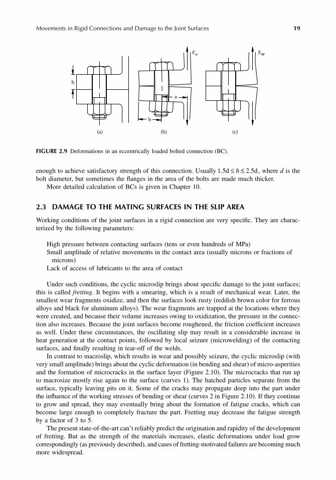
enough to achieve satisfactory strength of this connection. Usually , where d is thebolt diameter, but sometimes the flanges in the area of the bolts are made much thicker.
More detailed calculation of BCs is given in Chapter 10.
2.3 DAMAGE TO THE MATING SURFACES IN THE SLIP AREA
Working conditions of the joint surfaces in a rigid connection are very specific. They are charac-terized by the following parameters:
High pressure between contacting surfaces (tens or even hundreds of MPa)Small amplitude of relative movements in the contact area (usually microns or fractions of
microns)Lack of access of lubricants to the area of contact
Under such conditions, the cyclic microslip brings about specific damage to the joint surfaces;this is called fretting. It begins with a smearing, which is a result of mechanical wear. Later, thesmallest wear fragments oxidize, and then the surfaces look rusty (reddish brown color for ferrousalloys and black for aluminum alloys). The wear fragments are trapped at the locations where theywere created, and because their volume increases owing to oxidization, the pressure in the connec-tion also increases. Because the joint surfaces become roughened, the friction coefficient increasesas well. Under these circumstances, the oscillating slip may result in a considerable increase inheat generation at the contact points, followed by local seizure (microwelding) of the contactingsurfaces, and finally resulting in tear-off of the welds.
In contrast to macroslip, which results in wear and possibly seizure, the cyclic microslip (withvery small amplitude) brings about the cyclic deformation (in bending and shear) of micro-asperitiesand the formation of microcracks in the surface layer (Figure 2.10). The microcracks that run upto macrosize mostly rise again to the surface (curves 1). The hatched particles separate from thesurface, typically leaving pits on it. Some of the cracks may propagate deep into the part underthe influence of the working stresses of bending or shear (curves 2 in Figure 2.10). If they continueto grow and spread, they may eventually bring about the formation of fatigue cracks, which canbecome large enough to completely fracture the part. Fretting may decrease the fatigue strengthby a factor of 3 to 5.
The present state-of-the-art can’t reliably predict the origination and rapidity of the developmentof fretting. But as the strength of the materials increases, elastic deformations under load growcorrespondingly (as previously described), and cases of fretting-motivated failures are becoming muchmore widespread.
FIGURE 2.9 Deformations in an eccentrically loaded bolted connection (BC).
(a) (b) (c)
a
b
Fw Fw
h
1.5d 2.5d≤ ≤h
9563_C002.fm Page 19 Wednesday, July 25, 2007 4:05 PM

20 Machine Elements: Life and Design
Structural and technological means to increase the durability of parts in areas of rigid connec-tions are aimed at achieving the following goals:
Increase of compressive stresses in the joint to prevent slip or at least diminish its amplitude.Formation of a thin intermediate layer between joint surfaces (for example, by means of
copper or lead coating) in order to avoid direct contact between two hard metals.Inducing residual compressive stresses in surface layers of parts (by means of shot peening
or burnishing — see Chapter 3); this treatment doesn’t prevent fretting, but cracks origi-nating in the surface layer don’t propagate deeply into the part, so the strength-harmingeffect of fretting damage may be neutralized partly or completely.
Surface hardening by means of nitriding, carburizing, or induction hardening; these treat-ments not only produce high compressive stresses in the hardened layer (because of greaterspecific volume of the hardened metal), but also increase by far the mechanical strengthof this layer and diminish the probability of crack initiation.
In movable joints (for example, in spline connections, or in gear-type couplings) working underload, relative immobility may result when high contact pressure and very small amplitude ofoscillating slip are simultaneously present. These conditions are similar to those in rigid joints, andthey also may result in fretting. For these joints, in addition to the methods described previously,friction in the connection may be diminished by making the lubricant flow through the connectionor by coating the surfaces with molybdenum disulfide (MoS2). These measures, however, can’t berecommended for rigid connections.
REFERENCES
1. Müller, H.W., Drehmoment-Uebertragung in Pressverbindungen, Konstruktion, 14, H.2 u.3, 1962 (inGerman).
2. Klebanov, B.M., Load transmission by press-fit connections between shafts and massive discs,Mechanics of Deformable Systems in Agricultural Engineering, collected articles, Rostov-na-Donu,1974 (in Russian).
3. Marshall, M.B., Dwyer, L.R., and Joyce, R.S., Characterization of contact pressure distribution inbolted joints, Strain, 42, 2006, Blackwell Publishing Ltd.
FIGURE 2.10 Strength-damaging effect of fretting.
2
2
1
1 2
Cyclic motion
9563_C002.fm Page 20 Wednesday, July 25, 2007 4:05 PM

21
3
Deformations and Stress Patterns in Machine Components
A school teacher took two pieces of lead, cleaned their surfaces with a knife, and pressed themstrongly against each other. The two pieces stuck together, and the teacher asked us to separatethem. We were little boys, and this was a hard job for us. In that way, the teacher had clearlydemonstrated to us the property of molecular adhesion. Now we have grown up, and we know thata metal is a complicated mass of crystals, grains, molecules, and atoms combined together by theforces of molecular and atomic bonding.
3.1 STRUCTURE AND STRENGTH OF METALS
Metals at a normal temperature are crystalline solids. The atoms in the crystals are located peri-odically and form a structure that represents a multitude of identical elements. If lines are drawnthrough the centers of atoms, these lines form a spatial lattice called
crystal lattice
. Metals andalloys used in engineering mostly have a cubic lattice. Figure 3.1a shows the elementary cube ofthe iron structure at a normal temperature. It is a body-centered cube (bcc) with atoms placed inthe corners and in the center. The length of the cube side
a
=
2.86 Å, that is, 2.86·10
−
7
mm. (Theunit Å is the Angström, a linear dimensional unit of convenient size for atomic-scale measurements.)
If the metal is alloyed, not all the places in the cube are filled with the parent metal, butsome of the places are taken by the alloying metal atoms. But this doesn’t change the followingconsiderations.
Figure 3.1b shows a small part of a perfect crystal lattice. Application of load (Figure 3.1c) deformsthe lattice, but the forces of atomic bonding resist the possible sliding of the atomic layers. When theexternal load ceases, the atomic forces restore the initial balanced condition of the lattice. It is clear thatthe external force can be big enough, so as to overcome the atomic bonding and to displace the atomiclayers by one step of the lattice. But this assumes that the entire layer of atoms would be moved at once.Calculations based on the strength of the atomic bonding show that the external force needed for thisto take place would be greater than the real strength of the material by a factor of 100 and more.Therefore, something must explain the disparity between theory and reality, and it is as follows.
Numerous investigations have disclosed that the reason for the degraded strength of materials(as compared to its theoretical value) is the imperfection of the crystal structure. Several kinds ofimperfection are shown in Figure 3.2:
Vacancies (Figure 3.2a), where one atom is absent.Interstitials (Figure 3.2b), where one atom has squeezed itself into the lattice.Edge dislocations (Figure 3.2c), where an incomplete row of atoms is squeezed into the
lattice (or, if you prefer to be more pessimistic, part of a row is missing).Screw dislocations. (The last consist of a row of atoms turned relative to the parent lattice by a
small angle; they have a 3-D form and therefore are more difficult for 2-D graphic presentation.)
Of the reasons given previously, the greatest reduction of strength is due to dislocations.Figure 3.3a shows an unloaded part of lattice with edge dislocation 1. Near the end of the dislocationthe crystal lattice is distorted, and some of the atomic bonding forces (for example, between atom2 (fully shaded) and atoms 3 and 4 (both are half-shaded) are weakened. When the load is applied
9563_C003.fm Page 21 Wednesday, July 25, 2007 4:09 PM

22
Machine Elements: Life and Design
FIGURE 3.1
Crystal cell and crystal lattice.
FIGURE 3.2
Crystal lattice imperfections.
FIGURE 3.3
Dislocation and its movement under load.
(c)(b)(a)
Shear load
a
(a) (b) (c)
(a) (b) (c)2
34 1
Slip plane
(d) (e)
9563_C003.fm Page 22 Wednesday, July 25, 2007 4:09 PM

Deformations and Stress Patterns in Machine Components
23
(Figure 3.3b), most of it is taken by the elastically displaced atomic rows, but, in addition, atom2, which has been already moved from atom 3 toward atom 4, jumps from 3 to 4, so that thedislocation moves to the right as shown in Figure 3.3b. This jerking (stepwise) motion continuesunder load until the dislocation goes out of the crystal (Figure 3.3c to Figure 3.3e). Thus, when adislocation exists, the force needed to displace the atomic rows by one atom spacing is quite small.The plane of displacement is called
sliding plane
or
slip plane
.The process of crystallization begins when the liquid metal is chilled somewhat below its
melting temperature. In the liquid metal appear lots of nuclei of crystallization, and the neighboringatoms attach to them. The crystals grow until they meet the neighboring crystals. In the end of thisprocess, which lasts several seconds, the metal passes into solid state in the form of a granularstructure (see Figure 3.4). Because, in the nuclei centers, the orientation of the initial cubes wasrandom, the same orientation remains in the grains of the solidified metal.
Figure 3.4 may give the impression that the quantity of the lattice cells in one grain is not sobig. This impression is false. Let’s calculate. The dimensions of the grains in steel, for example,range from about 0.015 mm (extra-fine-grained steel) to 0.220 mm (extra-coarse-grained). If wetake the finest grain, the quantity of the lattice cells in one row is given by
It is clear that the presentation of grains in Figure 3.4 exaggerates the size of the lattice cubesfor illustration.
The quantity of lattice cubes in 1 mm
3
is
FIGURE 3.4
Crystals and grains in the metal structure.
0 0152 86 10
5 24 107
4.
..
⋅= ⋅
−
9563_C003.fm Page 23 Wednesday, July 25, 2007 4:09 PM

24
Machine Elements: Life and Design
Among this astronomical amount, there may be millions of dislocations and other defectsinitiated by alien atoms, free electrons, grain boundaries, internal stresses, etc. When an externalload is applied, it induces stresses in the macrovolume of a part. These stresses have a certainpattern of direction and magnitude depending on the shape of the part, the kind of load, and theplace of load application. In the microvolumes in which the direction of the stresses coincides withthe direction of the slip planes of a grain, this grain may become plastically deformed by a verysmall amount, perhaps the magnitude of one atomic spacing (depending on the stress magnitude),owing to the movement of dislocations. Such “unlucky” crystals are always present, so metals withideal elasticity don’t exist; after even a small load is applied, some structural changes occurimmediately. This kind of submicrodeformation is related to such phenomena as energy loss inmaterials in the course of elastic deformation (so-called internal friction) and a time delay indeformation as compared to the applied load.
When the stress is big enough, the dislocations multiply, and at the yield stress, they multiplyvery intensively, causing plastic deformation of the metal. Lots of dislocations interfere with eachother, and their motion is hindered. This results in strengthening of the metal due to plasticdeformation.
Dislocations are generated under smaller stress as well. At a cyclic load, the dislocations areconstantly generated owing to movement on the grain boundaries and because of other processesin the crystal lattice, including their self-multiplication. The moving dislocations pile up on thegrain borders and may finally form a microcrack.
The description of the mechanism of plastic deformation and fatigue given previously is verymuch simplified. The dislocations can move not only straight in direction (horizontally), as shownin Figure 3.3, but they also can move around a closed polygon in the sliding plane and evenvertically (changing the sliding plane). The dislocations can unite within the crystal and divide itinto parts forming subgrains. The atomic-scale processes occurring in the metal under load aremultifarious in nature and are not yet studied enough to be used in strength calculations. But thisdescription shows that the metal is similar to living matter that feels the load applied and reacts toit by structural changes.
Thus, perfection of elasticity depends on the accuracy of measurements. But in practice, whenwe deal with macrostresses and macrodeformations, it is generally agreed (and it is accurate formost practical applications) that the metals are perfectly elastic until the stress reaches the yieldpoint; then it begins to get plastically deformed in macrovolumes, and the part changes its shape.
3.2 DEFORMATIONS IN THE ELASTIC RANGE
There is a linear dependence between stress and deformation called
Hooke’s law
. It means that ifwe know the stress magnitude and the modulus of elasticity of the material, we can calculate theelastic deformation of the stressed piece. On the other hand, when the deformation is known, thestresses can be easily determined. This dependence is the basis for most stress-measuring instru-ments; they measure deformations and translate them into stresses.
But there is one more field to which Hooke’s law can be applied: if we know (or are able tomake a true assumption about) the distribution of the deformations over the cross section of a part,we can calculate the maximal stress. To illustrate this idea, let’s consider the bending of a straightbeam. The so-called ‘‘engineering approach” to strength calculation of beams is based on thehypothesis of plane cross sections (PCS). The idea of this hypothesis is that the cross sections ofthe beam, which are plane before bending (Figure 3.5a), remain plane after bending (Figure 3.5b).With bending, the neighboring cross sections turn relative to each other by a certain angle
j
. The
12 86 10
4 27 107 3
19
( . ).
⋅= ⋅
−
9563_C003.fm Page 24 Wednesday, July 25, 2007 4:09 PM

Deformations and Stress Patterns in Machine Components
25
magnitude of this angle depends on the magnitude of the bending moment, the rigidity of the beamand, obviously, on the distance between the sections. Because the cross sections remain plane, thedeformation of the beam between them is a linear function of the height. Across the width of thebeam, the deformation doesn’t change (Figure 3.5c).
Let’s examine the word
hypothesis
. A hypothesis is a kind of assumption usually developed asfollows: If we desire to work out the relation between appearances to explain or predict phenomenaor processes and don’t have sufficient data to establish an exact dependence, we may begin bymaking some simplifying assumptions. Then, to check the validity of the hypothesis, these assump-tions and the dependence based on them are checked experimentally. If the correspondencebetween the experimental results and this invented dependence is not satisfactory, more appropriateassumptions should be made.
In our case, the hypothesis of PCS has been proved to be very exact and productive as appliedto beams of a uniform cross section. But there are some exceptions to this rule (as with all rules).For example, in the thin-walled beams shown in Figure 3.6, the stresses across the width are notuniform; hence, the plane cross sections become distorted after application of a load. Use offormulas based on the hypothesis of plane cross sections for such beams (with wide and thinflanges) may lead to a considerable error (the real stresses will be bigger than the calculated ones).But let’s get back to the usual case when this hypothesis works with high accuracy.
Figure 3.7a shows a rod with a rectangular cross section loaded by bending moment M. Thecross section of the rod is of variable height:
h
on the right and
H
on the left. A fillet of radius
r
makes the transition from the smaller height to the bigger one.First, let’s define the stresses in the right part of the rod, where the cross section is of constant
height
h
. For this part, the hypothesis of plane cross sections is valid. We consider a small element
FIGURE 3.5
Bending deformation of a straight beam.
FIGURE 3.6
Deformation of thin-walled beams with wide thin shelves or flanges.
MM
ϕ
(a)
(b)
(c)
9563_C003.fm Page 25 Wednesday, July 25, 2007 4:09 PM
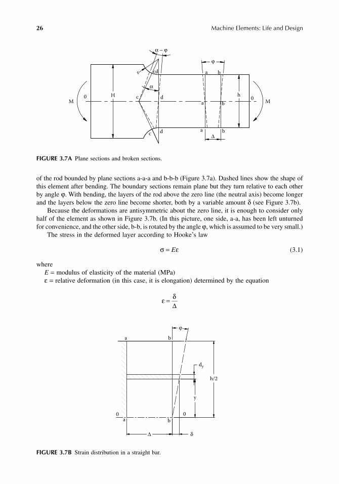
26
Machine Elements: Life and Design
of the rod bounded by plane sections a-a-a and b-b-b (Figure 3.7a). Dashed lines show the shape ofthis element after bending. The boundary sections remain plane but they turn relative to each otherby angle
ϕ
. With bending, the layers of the rod above the zero line (the neutral axis) become longerand the layers below the zero line become shorter, both by a variable amount
δ
(see Figure 3.7b).Because the deformations are antisymmetric about the zero line, it is enough to consider only
half of the element as shown in Figure 3.7b. (In this picture, one side, a-a, has been left unturnedfor convenience, and the other side, b-b, is rotated by the angle
ϕ
, which is assumed to be very small.)The stress in the deformed layer according to Hooke’s law
(3.1)
where
E
=
modulus of elasticity of the material (MPa)
ε
=
relative deformation (in this case, it is elongation) determined by the equation
FIGURE 3.7A
Plane sections and broken sections.
FIGURE 3.7B
Strain distribution in a straight bar.
r
α
H
ϕ
α − ϕ
∆a
a
b
b
c
cd
d
c d
a b M0 0
h
M
σ ε= E
ε δ=∆
b
∆
ϕ
0a
δ
h/2
dy
y
ba
0
9563_C003.fm Page 26 Wednesday, July 25, 2007 4:09 PM

Deformations and Stress Patterns in Machine Components
27
As is clear from the picture, the magnitude of
δ
depends on the ordinate
y
:
Therefore, the stress in each layer is proportional to the distance
y
of the layer from the zero line:
As the values
E
,
ϕ
, and
∆
are constant in this problem, all of them may be substituted by onecoefficient, say,
K
=
E
ϕ
/
∆
:
(3.2)
Now we are ready to calculate the stresses in this part of the rod. Elementary moment producedby a slice
dy
about the zero line
Here
b
=
thickness (width) of the rod (not shown in the picture).The sum of all the elementary moments, taken above and beneath the zero line, should be equal
to the loading moment
M
:
From here,
The maximal stress (at
y
=
h
/2) from Equation 3.2:
(3.3)
Fortunately, we didn’t make any mistakes and have got successfully the well-known equationfor a rod of a constant rectangular cross section. Now, let’s try to deal with the fillet area. In thisarea, the hypothesis of PCS doesn’t work. For this case, the hypothesis of broken-line cross sections(BCS) suggested by Verhovsky
1
works better. (The BCS hypothesis is based on experiments withrubber parts exposed to bending. The “cross sections” are just drawn on the side surface of therubber bar, so that their shape under bending can be easily observed.) According to this hypothesis,the cross sections, which continue to be plane, are directed at a perpendicular to the curvilinearsurface (section c-c-c, Figure 3.7a).
We consider a small element of the rod bounded by cross sections c-c-c and d-d-d (Figure 3.7a).This element is adjoined to the beginning of the fillet and characterized by an angle
α
that issupposed to be very small. Also, here the dashed lines show the shape of this element after bending.
δ ϕ= y
σ ϕ= Ey∆
σ = Ky
dM by dy Kby dy= ⋅ =σ 2
M dM Kbh
h
= =∫212
3
0
2/
KM
bh= 12
3
σmax ;= = =KyM
bhh
Mbh
122
63 2
9563_C003.fm Page 27 Wednesday, July 25, 2007 4:09 PM

28
Machine Elements: Life and Design
In the same way as the previous case, we consider only half of the small element (c-c-d-d, Figure 3.7c).One side of the element (c-c) is left unturned, and the other side, d-d, is rotated because of bendingby an angle
ϕ
. Notice that in this case, the elongation
δ
is also proportional to the ordinate
y
:
In the previous case, the length of the deformed layers
∆
was constant, whereas in this case,the length is variable and determined as follows:
This result is easily obtainable, if we take into consideration that the length of the elementarylayer depends linearly on its distance from point
e
. The layer with vertical coordinate
y
is at adistance of (
r
+
h
/2 –
y
) from point
e
. (Don’t forget: angle
α
is very small.)That is, in the element c-c-d-d not only do the deformations grow as the layers get farther from
the zero line, but also the length of the layers decreases, so the increase of the relative deformation(
ε
=
δ
/
∆
) with the increasing ordinate
y
is not linear but more intensive.The stress in the layer at a distance
y
from the zero line is
Because in this problem, values
E
,
α
, and
ϕ
are constant, they can be substituted by onecoefficient, say
L
=
E
ϕ
/
α
. Then the maximal stress (at
y
=
h
/2) is given by
(3.4)
FIGURE 3.7C
Strain distribution in a filleted bar.
e
c
c d0
d
dy
y
0
h/2
α−ϕ
ϕ
δ
α
∆
δ ϕ= y
∆ = + −( / )r h y2 α
σ ε δ ϕα
*
( / )= = =
+ −E E
Eyr h y∆ 2
σmax* = L
hr2
9563_C003.fm Page 28 Wednesday, July 25, 2007 4:09 PM

Deformations and Stress Patterns in Machine Components
29
The elementary moment produced by a slice
dy
about the zero line is given by
The sum of all the elementary moments should be equal to the loading moment
M
:
After the
L
value is derived from this equation and inserted in Equation 3.4, the followingformula for the maximal stress is obtained:
(3.5)
where
(3.6)
Let’s do comparative stress calculations for the straight part of the rod by Equation 3.3 and forthe beginning of the fillet by Equation 3.5 and Equation 3.6. For this calculation, we can take
b
=
h
=
1, because, for the comparison, it is not important if it is 1 mm or in. (or whichever unit oflength you want).
For the straight section, the maximal stress obtained from Equation 3.3 is
At the beginning of the fillet, the stress depends on the fillet radius. For example, if
r
=
0.2
h
,
Φ
=
0.1389, and the stress
The stress concentration factor Kt = 9/6 = 1.5. If the fillet radius r = 0.1h, Φ = 0.22, the maximal stress
and the stress concentration factor Kt = 11.36/6 = 1.89.Here, shown clearly (and even visually), is the mechanism of the local stress raise called stress
concentration. It is caused by a change in the shape of the machine component that modifies thedeformation pattern. The place where the shape changes is called a stress raiser (or stress riser).The sharper the change of the shape (in our case, the less the fillet radius), the higher the local stress.
dM by dy Ly b
r h ydy= ⋅ =
+ −σ
2
2/
M dM Lby
r h ydy Lb hr h
hh
= =+ −
= − −∫∫2 22
212
38
2
0
2
0
2
/
//
22 222
− ++
( / ) ln
/r h
rr h
σmax* = Mh
rb41
Φ
Φ = − − − ++
12
38
22
2 2hr h r hr
r h( / ) ln
/
σmax = 6M
σmax*
. .=
⋅⋅ =M
M4 0 2
10 1389
9
σmax*
. ..=
⋅⋅ =M
M4 0 1
10 22
11 36
9563_C003.fm Page 29 Wednesday, July 25, 2007 4:09 PM

30 Machine Elements: Life and Design
The BCS hypothesis is good for a visual presentation of the stress raiser mechanism. But itgives a correct result only when the bigger section is sufficiently larger than the smaller one, andthe stress raiser is not too sharp. Specifically, in the case considered previously, according to R. E.Peterson,3 Kt = 1.34–1.53 for r = 0.2h, and Kt = 1.48–1.93 for r = 0.1h depending on the ratio H/h.The BCS hypothesis doesn’t take into account this factor, and in our calculation we got Kt = 1.5and Kt = 1.89, respectively, i.e., close to the biggest values given by Peterson.
In most cases, the magnitude of the local stress can’t be determined by an analytical procedure.Experimental methods and FEM are usually used for this purpose.
Another application of the BCS hypothesis is with a flat strip of rectangular cross section, intension. If the strip is of constant cross section (Figure 3.8a), then obviously the hypothesis of PCSis valid. Under load, any small element of the strip bounded by sections a-a and b-b elongatesevenly across the width of the strip (see the dashed line).
Figure 3.8b shows a strip with semicircular notches that has the same width w (in the narrowsection). The cross sections, which keep their shape when loaded, look different (sections c-c andd-d). In the area of the notches, the length of the layers is significantly shorter than in the middleof the strip, and when section d-d is displaced under load (see dashed line), the relative elongationin this area will be greater. The stress distribution across the width of the strip will changecorrespondingly. Because in both cases the sum of all the stresses must be equal to the externalload, the maximal stress in the notched specimen will be greater than that in the straight strip.
Let’s discuss more fully the meaning of the stress concentration factor (SCF), because it isnot always clear. The maximal stress magnitude in the area of the stress raiser is determined usingtheory of elasticity techniques, by FEM, or experimentally. To calculate the SCF value, themaximal stress is divided by some “nominal” stress determined by methods of the strength ofmaterials (so-called engineering methods). For the rod shown in Figure 3.7a, the nominal stress isdetermined from Equation 3.3. For the strip presented in Figure 3.8b, the nominal stress is obviouslythe ratio of the stretching force to the minimal cross-sectional area (through the bottoms of thenotches). But if, for example, you are going to use SCF diagrams for a splined shaft, or a threadedshaft, or a shaft with a keyway, you have to figure out which cross section had been taken by theauthor when calculating the ‘‘nominal” stress: was it a circular cross section corresponding to theinner diameter of the teeth or thread, the real cross section, or something else? To calculate strengthof the machine part, you should know the maximal stress. For that you calculate the nominal stressand then multiply it by the SCF. So until you know which cross section should be taken for the‘‘nominal” calculation, you can’t use these diagrams.
FIGURE 3.8 Stress concentration in a notched strip in tension.
Tensile load
Stress
ba
W W
d d
(a) (b)
ba c c
9563_C003.fm Page 30 Wednesday, July 25, 2007 4:09 PM

Deformations and Stress Patterns in Machine Components 31
The SCF obtained from such calculations is called theoretical SCF (Kt), and it enables (inprinciple) the designer to determine the maximal stress. At this point, the mathematics comes toan end, and some uncertainty begins. The fact is that in the trials for strength, the load capacityof the machine members reduces not by Kt times but less, by Ke times. The Ke value is calledeffective SCF, and that is what we really need to know but can’t. The interrelation between Kt andKe is complicated and multifactored. Much depends on the loading condition. For example, undera static load, ductile materials (such are all the structural steels) are not sensitive to stress raisers.When the local stress comes up to the yield point, this brings about a local plastic deformationthat doesn’t harm the strength of the material but redistributes the stresses in such a way that theless-stressed volumes became more stressed in the elastic range. As the static load increases, theplastically deformed volume increases until it spreads across the whole section. This is the limitingstate under static load whether there is a stress raiser or not, and thus here, Ke = 1.
Under a cyclic load, the stress raisers reduce the load capacity of the machine parts, but lessthan the Kt value predicts, depending on the feature called sensitivity to stress concentration. Inpractice, the Ke value is often derived from the following equation:
where q is a coefficient of sensitivity to stress concentration.That coefficient depends on a number of factors:
The kind of material and existence in its structure of internal stress raisers (such as discon-tinuities in the form of foreign inclusions, defects on the grain boundaries, and disloca-tions). For instance, gray cast iron is hardly sensitive to sharp stress raisers under cyclicload, because its structure is pierced with flakes of graphite, which are sharp stress raisersincorporated into the material. And yet, the gray cast iron is sensitive to the stressconcentration under the static load, because it is brittle, and stresses can’t be effectivelyredistributed by local plastic deformations.
The ductility of the material: The less the ratio of the yield stress to the ultimate stress ofa steel, the less sensitive it is to the stress concentration. That means that high-strengthsteels are more sensitive to SCF.
The sharpness of the stress raiser: The sharper it is, the smaller the high-stressed volumeand the stronger the effect of the stress release owing to local plastic deformations (forexample, the sensitivity to the stress raiser is less).
The size of a part: Larger parts have greater (at the same sharpness of the stress raiser) high-stressed volume, yielding a less than helpful effect from local plastic deformation.
A host of other factors, such as quantity of load cycles and ratio of the mean stress to itsamplitude.
Because most of these factors are difficult to take into account, the recommendations forchoosing the q value are very approximate. But it is known that high-strength structural steels arevery sensitive to stress concentration under cyclic load, and the recommended q value for them isabout 0.90–0.95.
Some authors recommend (on the basis of experiments) coefficients Ke for a certain type ofstress raiser (for example, threaded or splined shafts) related to certain steels. But in very importantapplications, in which totally reliable information about the permissible load is needed, the actualparts should be tested for strength and durability under real loading conditions.
K q Ke t= + −1 1( )
9563_C003.fm Page 31 Wednesday, July 25, 2007 4:09 PM
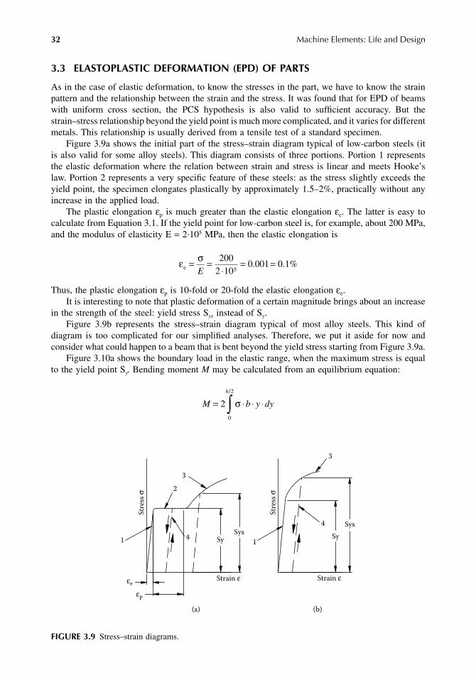
32 Machine Elements: Life and Design
3.3 ELASTOPLASTIC DEFORMATION (EPD) OF PARTS
As in the case of elastic deformation, to know the stresses in the part, we have to know the strainpattern and the relationship between the strain and the stress. It was found that for EPD of beamswith uniform cross section, the PCS hypothesis is also valid to sufficient accuracy. But thestrain–stress relationship beyond the yield point is much more complicated, and it varies for differentmetals. This relationship is usually derived from a tensile test of a standard specimen.
Figure 3.9a shows the initial part of the stress–strain diagram typical of low-carbon steels (itis also valid for some alloy steels). This diagram consists of three portions. Portion 1 representsthe elastic deformation where the relation between strain and stress is linear and meets Hooke’slaw. Portion 2 represents a very specific feature of these steels: as the stress slightly exceeds theyield point, the specimen elongates plastically by approximately 1.5–2%, practically without anyincrease in the applied load.
The plastic elongation εp is much greater than the elastic elongation εe. The latter is easy tocalculate from Equation 3.1. If the yield point for low-carbon steel is, for example, about 200 MPa,and the modulus of elasticity E = 2·105 MPa, then the elastic elongation is
Thus, the plastic elongation εp is 10-fold or 20-fold the elastic elongation εe.It is interesting to note that plastic deformation of a certain magnitude brings about an increase
in the strength of the steel: yield stress Sys instead of Sy.Figure 3.9b represents the stress–strain diagram typical of most alloy steels. This kind of
diagram is too complicated for our simplified analyses. Therefore, we put it aside for now andconsider what could happen to a beam that is bent beyond the yield stress starting from Figure 3.9a.
Figure 3.10a shows the boundary load in the elastic range, when the maximum stress is equalto the yield point Sy. Bending moment M may be calculated from an equilibrium equation:
FIGURE 3.9 Stress–strain diagrams.
ε σe = =
⋅= =
E200
2 100 001 0 1
5. . %
M b y dy
h
= ⋅ ⋅ ⋅∫20
2
σ/
Str
ess
σ
Strain ε
1
2
(a) (b)
1
3
Strain ε
Str
ess
σ
4
4
3
εp
εe
SySys
Sys
Sy
9563_C003.fm Page 32 Wednesday, July 25, 2007 4:09 PM

Deformations and Stress Patterns in Machine Components 33
where b = width of the beam (not shown in the figure)σ = stress at a distance y from the zero line
From this
What will happen if the load is increased? As said earlier, the hypothesis of plane cross sectionsis valid in this case as well. That means that the angle ϕ between the two neighboring cross sections(Figure 3.7a and Figure 3.7b) will grow, and the layers will be additionally elongated by an amountthat is proportional to the distance y of the layer from the zero line. But the deformation of thelayers most distant from the zero line will grow without increase in stress beyond the yield point.Figure 3.10b shows the situation in which deformation is twice as much as in Figure 3.10a. In thiscase, the yielding area begins at y = h/4 and extends to y = h/2. The equilibrium equation for this case is
FIGURE 3.10 Deformation of a beam in elastic and elastoplastic ranges.
(a)
εe
M M
1.375 εe
(c)
123
12 3
c
d
e
f
g
h
a
b
TensionCompressionSy
(d)
a
b
0.375 εe
0.375 Sy
εe
(e)
k
l
m
n
0.625 εe
0.625 Sy
0.81 εe
0.81 Sy
Sy
dyy
h/2
(b)
1.375 M 1.375 Mh
Sy
h/4
σ = Sy
hy
2
M S b hy= ⋅16
2
M Sy
hb y dy S b y dy Sy
h
y
h
h
∗ = ⋅ ⋅ + ⋅ ⋅ =∫ ∫24
21148
0
4
4
2/
/
/
yyb h⋅ 2
9563_C003.fm Page 33 Wednesday, July 25, 2007 4:09 PM

34 Machine Elements: Life and Design
As we can see, bending moment M* is greater than M:
Hence, if such a yield that covers half of the cross-sectional area is permissible, the bendingmoment may be increased by 37.5%.
There may be some doubt about the plastic deformation in this case: is it still relatively smallor is the metal deformed too much and already beginning to break? As we saw earlier, the maximumelastic deformation εe is about 0.1%. In our case, this layer is placed at a distance of h/4 from thezero line. The maximal deformation, elastic and plastic (at a distance of h/2), in accordance withthe plane cross sections hypothesis, is twice as much, i.e., 0.2%. Half of this amount (0.1%) is theelastic deformation that remains in the material, and the other half is the plastic deformation. Thismagnitude of plastic deformation is very small and cannot yet impair the mechanical properties ofthe metal.
A comparison of Figure 3.10a and Figure 3.10b demonstrates clearly that the plastic deformationof layers more distant from the zero line brings about increased loading of the layers at a shorterdistance from the zero line. So, the summary moment of the internal forces about the neutral axisof the cross section is obviously greater in the case of EPD.
It should be noticed, however, that the gain in load capacity (37.5%) was calculated for a beamwith rectangular cross section (Figure 3.11b). If the beam is of a round cross section (Figure 3.11c),the increase in load capacity should be greater, because the layers become wider as they are closerto the zero line. For an I-beam (Figure 3.11d), though, EPD is less effective because the crosssection is thin in the middle portion, and additional stressing does not add much.
Plastically deformed metal behaves in the same manner as the initial one: as it is unloaded, itfollows Hooke’s law with the same modulus of elasticity (line 4 in Figure 3.9a, arrow downwards).When loaded again, it follows the same line (arrow upwards) until it comes to the yield stress andcontinues plastic deformation as if the process of unloading and repeated loading has not beenperformed. This feature, plus the validity of the PCS hypothesis for EPD, allows us to predict theresidual stress pattern in deformed machine parts. For example, after the beam was loaded in theelastoplastic range according to Figure 3.10b and then unloaded, the plastically deformed layersdidn’t allow the elastically deformed layers (in the middle of the section) to return to their initialstate. This counteraction results in a balanced system of residual stresses in the unloaded beam.The distribution of these stresses may be found by superposition of deformations. Figure 3.10cshows the distribution of deformation over the height of the cross section when loaded by a positivelydirected bending moment of 1.375M (Figure 3.10b). Areas 1 (lines c-d-e-f) show the elastic portionof deformation, and areas 2 represent the plastic portion. The last doesn’t take part in subsequent
FIGURE 3.11 The effectiveness of elastoplastic deformation.
MM
*
.= ⋅ =11 648
1 375
(a) (b) (c) (d)
9563_C003.fm Page 34 Wednesday, July 25, 2007 4:09 PM
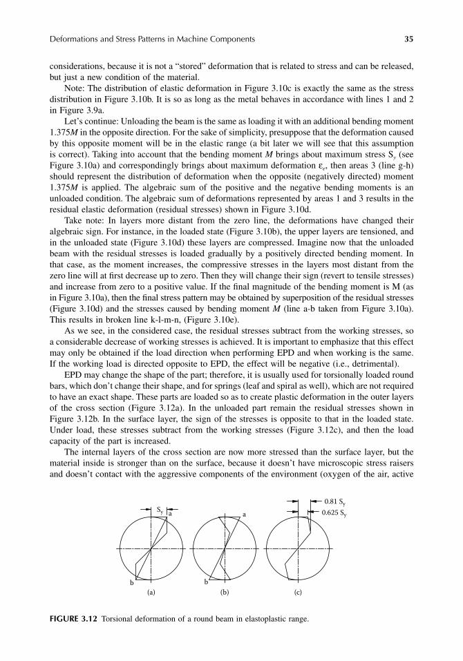
Deformations and Stress Patterns in Machine Components 35
considerations, because it is not a “stored” deformation that is related to stress and can be released,but just a new condition of the material.
Note: The distribution of elastic deformation in Figure 3.10c is exactly the same as the stressdistribution in Figure 3.10b. It is so as long as the metal behaves in accordance with lines 1 and 2in Figure 3.9a.
Let’s continue: Unloading the beam is the same as loading it with an additional bending moment1.375M in the opposite direction. For the sake of simplicity, presuppose that the deformation causedby this opposite moment will be in the elastic range (a bit later we will see that this assumptionis correct). Taking into account that the bending moment M brings about maximum stress Sy (seeFigure 3.10a) and correspondingly brings about maximum deformation εe, then areas 3 (line g-h)should represent the distribution of deformation when the opposite (negatively directed) moment1.375M is applied. The algebraic sum of the positive and the negative bending moments is anunloaded condition. The algebraic sum of deformations represented by areas 1 and 3 results in theresidual elastic deformation (residual stresses) shown in Figure 3.10d.
Take note: In layers more distant from the zero line, the deformations have changed theiralgebraic sign. For instance, in the loaded state (Figure 3.10b), the upper layers are tensioned, andin the unloaded state (Figure 3.10d) these layers are compressed. Imagine now that the unloadedbeam with the residual stresses is loaded gradually by a positively directed bending moment. Inthat case, as the moment increases, the compressive stresses in the layers most distant from thezero line will at first decrease up to zero. Then they will change their sign (revert to tensile stresses)and increase from zero to a positive value. If the final magnitude of the bending moment is M (asin Figure 3.10a), then the final stress pattern may be obtained by superposition of the residual stresses(Figure 3.10d) and the stresses caused by bending moment M (line a-b taken from Figure 3.10a).This results in broken line k-l-m-n, (Figure 3.10e).
As we see, in the considered case, the residual stresses subtract from the working stresses, soa considerable decrease of working stresses is achieved. It is important to emphasize that this effectmay only be obtained if the load direction when performing EPD and when working is the same.If the working load is directed opposite to EPD, the effect will be negative (i.e., detrimental).
EPD may change the shape of the part; therefore, it is usually used for torsionally loaded roundbars, which don’t change their shape, and for springs (leaf and spiral as well), which are not requiredto have an exact shape. These parts are loaded so as to create plastic deformation in the outer layersof the cross section (Figure 3.12a). In the unloaded part remain the residual stresses shown inFigure 3.12b. In the surface layer, the sign of the stresses is opposite to that in the loaded state.Under load, these stresses subtract from the working stresses (Figure 3.12c), and then the loadcapacity of the part is increased.
The internal layers of the cross section are now more stressed than the surface layer, but thematerial inside is stronger than on the surface, because it doesn’t have microscopic stress raisersand doesn’t contact with the aggressive components of the environment (oxygen of the air, active
FIGURE 3.12 Torsional deformation of a round beam in elastoplastic range.
(a)
aSy
(b) (c)
b
a
0.81 Sy
0.625 Sy
b
9563_C003.fm Page 35 Wednesday, July 25, 2007 4:09 PM

36 Machine Elements: Life and Design
additives to the lubricants, and others). So the surface layers remain the potential trouble spot, butthey become less stressed.
Not all materials have a “plateau” (line 2 in Figure 3.9a) in their strain–stress diagrams.Figure 3.9b shows the strain–stress diagram typical for most of the alloyed steels. It doesn’t changethe principle of EPD, but the stress distribution is different (Figure 3.13). The residual stress patternshould be determined relying on the real strain–stress diagram of the material used.
It is important to note that the plastic deformation is not a momentary process; it takes timeto change the structure of the material. Therefore, when carrying out EPD, the part is usually heldin a deformed state for some time, or the deformation is repeated several times.
3.4 SURFACE PLASTIC DEFORMATION (SPD)
As we have seen previously, useful EPD may be done only if the working load is of constantdirection relative to the part. At that, the direction of the load vector relative to other objects, suchas the housing, the ground, and the like, should not be considered. For example, a radial forceapplied to a shaft from gear teeth is of constant direction relative to the housing, but the shaft isrotating, so the vector of the bending moment rotates with reference to the shaft. As this takesplace, each point of the shaft is loaded alternately in tension and in compression, and the EPD bybending in any direction can’t help but make the shaft crooked. In this case, it is useful to induceresidual compressive stresses in the surface layer of the part — throughout or in the high-stressedportion of it.
Just a minute! A careful reader might say. If there is a residual compressive stress in the surfacelayer and the working stress changes cyclically from tension to compression, the stresses willalternately subtract and add. So the maximum tension stress will be less but the maximum com-pressive stress will be greater than without any residual stresses.
Yes, that is what is going to happen. But, what should be taken into account here is that thestrength of steels is identical in compression and in tension, but only under a constant load. Undercyclic load, when materials fail by fatigue, it is not so.
Investigators made fatigue tests of T-shaped beams (Figure 3.14) bent by pulsating moment M.The direction of the bending moment was chosen so as to have the compressive stresses greaterthan the tension stresses. The needed relation between these stresses was achieved by controllingthe width of flange W. (The wider the flange, the lower is the position of the neutral axis and the
FIGURE 3.13 Torsional deformation of a round beam that yields according to Figure 3.9b.
Sy
9563_C003.fm Page 36 Wednesday, July 25, 2007 4:09 PM

Deformations and Stress Patterns in Machine Components 37
less the tension stress as compared to the compressive stress.) The fatigue cracks that appearedwere mostly on the tensioned side. On the compressed side, cracks were obtained only when thecompressive stress was about twice the magnitude of the tensile stress. Consequently, the fatiguestrength of steels may be increased by decreasing the tensile stresses, even at the cost of anincrease of the compressive stresses. But if the total compressive stress exceeds the yield pointof the material, the residual stress decreases. The mechanism of residual stress loss is discussedin the following text.
The two methods most commonly used for SPD are burnishing (with balls or rollers) and shotpeening. When burnishing, the surface layer is rolled out like dough on a table. To let the doughexpand freely, the cook powders the table with flour. But in our case, the “table” (the layersunderneath the plastically deformed layer) is bonded with the “dough” and resists its expansion.The interaction between them creates some balanced system of internal stresses: compressive inthe surface layer and tension underneath it (Figure 3.15). In addition to the compressive residualstress, the plastically deformed layer is somewhat stronger (see Figure 3.9). These two factorsenable increase in the load capacity of the parts.
FIGURE 3.14 Bending stresses in a T-beam.
FIGURE 3.15 Residual stress distribution after shot peening or cold rolling.
M M
0 0
Compressive stress
Tensile stress
W
Compressive stressTensile stress
9563_C003.fm Page 37 Wednesday, July 25, 2007 4:09 PM

38 Machine Elements: Life and Design
The burnishing roller should be pressed against the surface by a force that depends on thestrength of the material, the diameters of the part and the roller, and the desired thickness of thedeformed layer. The larger the diameter of the part, the thicker (as a rule) the plastically deformedlayer should be (millimeters or even centimeters) to achieve a considerable increase in strength.
The shape of the roller also depends on the shape of the burnished surface. Usually, the workingsurface of the roller is shaped to a circular form (Figure 3.16a and Figure 3.16b), sometimes witha cylindrical portion (Figure 3.16c). To burnish a fillet, the radius of the roller profile should beless than the fillet radius. Figure 3.16d shows a special profile roller for burnishing fillets2: whenthe tool rotates with the shaft, the changing profile of the roller surface causes the contact pointsto alternately sweep from the center of the fillet to the sides, and back to the center. In this way,the contact spots of the fillet with the roller cover the entire surface of the fillet.
The same goal (creation of plastically deformed layer with residual compressive stress) isachieved by shot peening. A stream of hard spherical shots strikes the surface of the part at highvelocity. Each shot dents the surface and produces a small plastic deformation. Thousands of shotscreate a plastically deformed layer. Its thickness doesn’t exceed 0.4 – 0.5 mm. After shot peening,the surface has a specific “pock-marked” appearance. The geometry of the shot-peened surfaceschanges slightly, requiring those surfaces that have to be exact and smooth (such as shaft necksfor bearings) to have subsequent fine machining, usually grinding. This process may be harmfulbecause heating is inevitable while grinding and may relax the residual compressive stress andeven change it to tension stress. The result of the machining can’t be controlled by nondestructivemethods, and this reduces the reliability of this process.
Shot peening is successfully used for parts of complicated shape that can’t be burnished anddon’t have to have an exact surface, such as springs, engine connecting rods, etc.
Burnishing allows creating a much thicker plastically deformed layer than shot peening, and,in case subsequent grinding is needed, the local overheating is much less dangerous. Besides, thesurface after burnishing is very smooth, so that for some surfaces (for example, threads) SPD viaburnishing may eliminate the need for further processing. And what is more, small and midsizedthreads are usually formed by rolling, without any cutting tools.
Finally, let’s discuss the issue of the possible loss of residual stress.Figure 3.17a shows a very simplified stress distribution in the initial state: the part is unloaded,
and in the shot-peened layer, there is a residual compressive stress σr that equals approximately0.5Sy (Sy is the yield point). Under this layer, there are tension stresses of relatively smallmagnitude. Dashed line 1 represents the stress pattern caused by bending the part with moment M.The sum of the two patterns shown in Figure 3.17b represents the stress distribution in the loadedpart. In the lower portion of the part, the compressive residual stress σr subtracts from the tensionbending stress σb, and this results in a sharp decrease of the stress in this layer. In the upper portion
FIGURE 3.16 Shapes of typical rollers for burnishing shafts.
(a) (b) (c) (d)
9563_C003.fm Page 38 Wednesday, July 25, 2007 4:09 PM

Deformations and Stress Patterns in Machine Components 39
of the part, the compressive residual stress σr and the compressive bending stress σb are additive,and their sum exceeds Sy. But in the material, the yield stress can’t be exceeded at this magnitudeof strain, and part of this sum (marked 2) is cut off. After the part is unloaded, the residual stressin the upper portion becomes less by exactly the cut off piece 2 (Figure 3.17c). In the lower portion,the residual stress remains the same until the part is bent in the opposite direction (Figure 3.17d).Then, the residual stress will be lost in the lower portion as well.
If the sum σr + σb doesn’t exceed the yield stress, the residual compressive stress in theplastically deformed layer remains unchanged.
REFERENCES
1. Verhovsky, A.V., Broken cross-section hypothesis and its application to calculation of bars of com-plicated shape, Transactions of Tomsk Polytechnic Institute on the Name of S. M. Kirov, Vol. 61/1,Tomsk, 1947 (in Russian).
2. Almen, J.O. and Black, P.H., Residual Stresses and Fatigue in Metals, McGraw-Hill, New York,San Francisco, Toronto, London.
3. Peterson, R. E., Stress Concentration Factors, John Wiley & Sons, New York, London, Sydney,Toronto, 1974.
FIGURE 3.17 Loss of residual stress due to reversed bending.
M
σr
σr + σbσb
1
Sy
2
(a) (b)
(c) (d)
M
Residual tensile
stress
9563_C003.fm Page 39 Wednesday, July 25, 2007 4:09 PM

9563_C003.fm Page 40 Wednesday, July 25, 2007 4:09 PM

Part II
Elements and Units of Machines
When designing a new machine, we usually start by looking for a patent and other informationabout what has been done in this field. It is a rare case when we need to make something completelynew. Generally, we can often find a machine in service that closely meets our needs as evidencedby its function (and sometimes also by parameters such as capacity, output etc.). Such a machineis called a
prototype
.The only documentation available for our prototype is often just a data sheet or some servicing
instructions, and it may be difficult to obtain. So it definitely would be advantageous to go to theprototype and study it in service. In that way we begin to obtain more of an idea of the similarmachine that we are to create.
What next? Let us suppose that we like the prototype, and it is highly desirable (in order to savetime and money) to follow its design as closely as possible. We have only some visual information,and we will have to fill in the missing information using our own abilities. In other words, tounderstand, interpret and replicate the design of the prototype in every detail depends completely onour knowledge, our experience, and the intuition (called “mechanical aptitude”) that we have devel-oped from the experience.
Unfortunately, even if we know something, we may forget about it; also we can miss it whenconsidering the numerous factors and options of the design. If it isn’t at the forefront of our mind,there is little chance to think of it at the right time. Therefore, there is no substitute for studyingtypical design features of units and details beforehand, for future use. If practiced frequently, thisshould bring the intimate knowledge that becomes part of an instinctive feeling for the right solution.This is what Part II is all about.
9563_C004.fm Page 41 Wednesday, July 25, 2007 4:10 PM

9563_C004.fm Page 42 Wednesday, July 25, 2007 4:10 PM

43
4
Shafts
4.1 SELECTING THE BASIC SHAFT SIZE
A shaft is a straight, mostly round bar, which is designed to have other rotating parts of a mechanismmounted on it. To function as such, the shaft may include splines and keyways to transmit torque,journals for rolling or sliding bearings, cylindrical and conical sections, threads, shoulders, and soon. Some elements that are commonly made as separate items (e.g., pinions, cams, connectingflanges) are often made instead as integral parts of the shaft.
Sometimes a shaft is not a part of a mechanism but serves as a connection between mechanismsor machines placed at a distance from each other. Such a shaft, called
intermediate
, must be providedwith elements transmitting torque on its ends; these are, as a rule, flanges, or splines, or necks forcouplings.
Although the shape of a shaft depends on the kind and features of the elements adjoined toor mounted on it, the size (or, rather, the diameter) of the shaft is mainly dictated by strengthconsiderations. Not only the strength of the shaft’s body but also the strength of the connectionstransmitting torque and radial forces, necessary diameters of bearing journals, etc., should alsobe considered. All these elements should be designed as component parts of a unit. Then, theelements of the shaft should be proportioned so as to avoid large, and/or abrupt differences(changes) in diameter. This may be achieved by selecting a suitable material and heat treatment,changing relations between diameter and length of connections and journal bearings, varying typesand dimensions of rolling bearings, changing types of connections (e.g., spline, key, or flange),and by other means. All in all, the process of designing a shaft is an integral part of designingthe whole mechanism.
In this iterative process, it is important to make an initial appraisal of the shaft diameter aslimited by its strength. The diameter may vary over a wide range depending on environmentalconditions, materials used, heat treatment, surface treatment, thoroughness of smoothing out thestress concentrators, and other factors. Tentatively, for the beginning of design, the diameter of ashaft loaded with a torque and bending moments, and with stress raisers such as shoulders, keyways and the like can be estimated from:
(4.1)
where
T
=
transmitted torque (N·mm)
S
u
=
tensile strength of the shaft material (MPa)
The diameter of a shaft that is loaded with torque only and doesn’t have considerable stressraisers may be as small as one half of the above:
(4.2)
d toTSu
≈ ( )5 6 3
d toTSu
≈ ( . )2 5 3 3
9563_C004.fm Page 43 Wednesday, July 25, 2007 4:10 PM

44
Machine Elements: Life and Design
E
XAMPLE
4.1
A shaft transmits a torque of 15,000 N·m. In addition, it is loaded by bending moments generatedby gears and couplings. The tensile strength of the shaft material
S
u
=
930 MPa. The shaft hasstress raisers such as press-fit connections, keyways, and shoulders. Limited by fatigue strength,the diameter of the shaft should be approximately equal to
It should be clear that this approximate estimation can’t replace the accepted strength calcula-tion, and the shaft must finally be checked for strength. In some cases, the equations cited earlierare inapplicable, for example, when the torque is about zero (see Figure 6.3 and Figure 6.24). Thediameter of each axle in these figures is determined by the inner diameter of the planet wheelbearing and by the bending strength of the axle, which is loaded by the gear teeth forces.
Although decreasing the dimensions of shafts is essential in the effort to limit weight, designersusually don’t use the strongest material for the first design of a new mechanism, and there are threereasons for that. First, such materials are noticeably more expensive and more difficult in machining,and that raises the price. Second, unanticipated loads may be present, which result in breakdowns,forcing a redesign with an increase in shaft strength as the objective. Third, sometimes the customerwants to use the mechanism for greater loads and asks the manufacturer to increase its load rating.In these occurrences, the increase of the shaft diameter is usually undesirable, because it results inchanging the mating parts, often including the housing. This increases by far the upgrade expenses.If alternatives are available, such as using some stronger material, application of surface hardening(carburizing or nitriding) and cold working, they will save a great deal of expense and effort inthese situations.
Sometimes there is no alternative but to increase the shaft diameter to satisfy rigidity or stabilityrequirements, mount larger bearings, or increase the load capacity of connections between the shaftand the attached parts.
E
XAMPLE
4.2
Figure 4.20 depicts the main shaft of a subway tunnel escalator. Forces
F
cu
and
F
cl
, estimated indozens of tons, load each of the two hauling sprockets. The diameters of the bearing necks of theshaft have been defined by the bearing’s inner diameter. The diameter of the shaft between thesprockets, as calculated in compliance with the strength requirements, shall be of about 250 mm.(See dashed lines in Figure 4.20.) But in this case, the elastic bending of the shaft will result ininadmissible tooth misalignment in the reduction gear. To avoid this defect, the shaft diameter hasbeen increased to 450 mm. Calculation of the resilience of this shaft is cited in Section 4.4.
Shafts, which are increased in diameter for the sake of rigidity, can be made of less strong (andconsequently cheaper) materials. But even in these cases, the use of soft steels with hardness ofHB 140–160 is not a good choice. While assembling tight or press fits, the mounting surfaces maybe damaged (i.e., scored or crushed), and the shaft may be bent. An accidental hit with a hardobject may leave a remarkable dent on such a shaft. In service, a short-term overload may causeturning of the inner race of a rolling bearing relative to the shaft neck. The soft material of theshaft will be worn away a bit, the bearing fit will become weaker, and the bearing unit will beunable to work (see Chapter 6, Section 6.2).
If the soft shaft is made as an integral part with a flange, the latter may be damaged whiletightening bolts (see Chapter 10, Section 10.1). For these and other reasons as well, it is desirablethat the shaft be sufficiently hard.
d to to mm≈ ⋅ =( )5 615000 10
930125 150
33
9563_C004.fm Page 44 Wednesday, July 25, 2007 4:10 PM
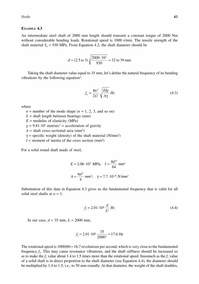
Shafts
45
E
XAMPLE
4.3
An intermediate steel shaft of 2000 mm length should transmit a constant torque of 2000 Nmwithout considerable bending loads. Rotational speed is 1000 r/min. The tensile strength of theshaft material
S
u
=
930 MPa. From Equation 4.2, the shaft diameter should be
Taking the shaft diameter value equal to 35 mm, let’s define the natural frequency of its bendingvibrations by the following equation
1
:
(4.3)
where
n
=
number of the mode shape (
n
=
1, 2, 3, and so on)
L
=
shaft length between bearings (mm)
E
=
modulus of elasticity (MPa)
g
=
9.81·10
3
mm/sec
2
=
acceleration of gravity
A
=
shaft cross-sectional area (mm
2
)
γ
=
specific weight (density) of the shaft material (N/mm
3
)
I
=
moment of inertia of the cross section (mm
4
)
For a solid round shaft made of steel,
Substitution of this data in Equation 4.3 gives us the fundamental frequency that is valid for allsolid steel shafts at
n
=
1:
(4.4)
In our case,
d
=
35 mm,
L
=
2000 mm,
The rotational speed is 1000/60
=
16.7 revolutions per second, which is very close to the fundamentalfrequency
f
1
. This may cause resonance vibrations, and the shaft stiffness should be increased soas to make the
f
1
value about 1.4 to 1.5 times more than the rotational speed. Inasmuch as the
f
1
valueof a solid shaft is in direct proportion to the shaft diameter (see Equation 4.4), the diameter shouldbe multiplied by 1.4 to 1.5, i.e., to 50 mm roundly. At that diameter, the weight of the shaft doubles,
d to≈ ⋅ =( . )2 5 32000 10
93032 39
33 to mm
fn
L
EIg
AHzn = π
γ
2
22
E Id
Ad
= ⋅ =
= = ⋅ −
2 06 1064
47 7 10
54
4
22
. ;
; .
MPa mm
mm
π
π γ 55 3N mm/
fdL
Hz16
22 01 10= ⋅.
f1 62
2 01 1035
200017 6= ⋅ =. . Hz
9563_C004.fm Page 45 Wednesday, July 25, 2007 4:10 PM

46
Machine Elements: Life and Design
from 15 kg to 30 kg. If the weight is limited, the shaft should be made hollow, for example,diameters outside (
d
o
) and inside (
d
i
) may be chosen as
d
o
/
d
i
=
40/30 mm or 45/38 mm. (Thesediameters are calculated so as to keep the same section modulus as for the solid shaft of 35 mmin diameter.) Substituting the data of these sections in Equation 4.3 gives us the following valuesof fundamental frequency:
For section 40/30 mm,
f
1
=
25.1 HzFor section 45/38 mm,
f
1
=
29.6 Hz
Thus, the fundamental frequencies of the hollow shafts are greater than the rotational speed by afactor of 1.55 and 1.77. An additional benefit is that the weight is less (than that of the solid shaftof 35 mm diameter) by a factor of 1.7 and 2.0, respectively.
Striving for further decrease in weight may lead to a thin-walled shaft. For instance, at diametersof
d
o
/
d
i
=
75/73 mm (wall thickness is of 1 mm), the weight of the hollow shaft is only 25% ofthat of the solid one. But the ratio of the wall thickness
t
to the mean radius
r
of the wall [
r
=
(
d
o
+
d
i
)/4] is now
r
/
t
=
37. Because this ratio is bigger than 10, the shaft should be checked forbuckling. In our case, the shaft is loaded with a torque only, so the critical (for stability in torsion)shear stress may be obtained from the following equation
2
:
As mentioned,
r
=
37 mm,
t
=
1 mm, so the critical stress is
The actual value of the shear stress
As we see, the actual shear stress is bigger than the critical one. That means that the hollowshaft with diameters 75/73 mm may buckle under load, and its dimensions should be changed soas to keep the actual shear stress not bigger than about half of its critical value.
Desirable changes in weight, stiffness, and the natural frequencies of a shaft may also beattained by changing the material properties, for example, by using titanium or aluminum alloysinstead of steel. The permissibility of this replacement should be considered with respect to allelements of the shaft, such as splines, bearing necks, and others.
4.2 ELEMENTS OF SHAFT DESIGN
Figure 4.1 shows a shaft with other parts mounted on it: a gear wheel, two bearings, a sleeve, a nut,and a half-coupling. This shaft has several sections of differing diameters. The stepped change ofthe shaft diameter from 150 mm to 140 mm provides shoulders, which represent location surfacesnecessary for the proper installation of the gear wheel and roller bearing. The change in diameterfrom 140 mm to 135 mm is required because of the difference in fit tolerances for the roller bearingand the half-coupling. The latter should have a press-fit connection with the shaft, whereas the rollerbearing needs a much lighter fit. If the nominal diameters of these two connections were the same,
τcr Etr
=
0 251 5
..
τcr = ⋅ ⋅
=0 25 2 06 101
372295
1 5
. ..
MPa
τπ πact
Tr t
= = ⋅⋅ ⋅
=2
2000 102 37 1
2332
3
2MPa
9563_C004.fm Page 46 Wednesday, July 25, 2007 4:10 PM

Shafts
47
the bearing would have been pushed (during assembly) through and beyond the half-coupling seat,and the increased interference while passing through this place would cause assembly problems.
In Figure 4.1, the diameter of the half-coupling seat is decreased to the nearest standard value(135 mm). But if a strength problem is encountered when using a round dimension and standardfit, the half-coupling seat can be made of the same diameter with the same tolerances as the bearingseat. The needed interference for the half-coupling fit should be achieved in that case by selectingan appropriate tolerance for the opening (bore) of the half-coupling.
Places where the section of the shaft is changing are also the places of stress concentration(see details in Chapter 3), and the sharper (more abrupt) the change in cross section, the strongerthe effect of stress concentration. A smoother change of shaft sections is achieved by settingsufficiently large fillet radii.
Although the influence of fillet radii on stress concentration factors is well known, the authorsin their practice have often seen drawings of shafts in which the fillet radii were dimensioned toosmall or even were not specified at all. When a designer is dimensioning a shoulder for a rollingbearing (Figure 4.2a), he usually takes the fillet radius from the bearing’s catalog prescriptions.
FIGURE 4.1
Gear output shaft.
FIGURE 4.2
Various shaft shoulders and fillets.
∅135r6/H6∅140n6∅140r6∅140m6
∅155h11
A B
(c) (d)(a) (b)
Point of interference
and possible damageIncorrect
9563_C004.fm Page 47 Wednesday, July 25, 2007 4:10 PM

48
Machine Elements: Life and Design
The designer keeps in mind that if the fillet radius is bigger than the chamfer on the inner race of thebearing (Figure 4.2b), the bearing will be mounted incorrectly, possibly with a skewness about theshaft axis. (Such a condition could lead to more than just misalignment or vibration, for the bearingmay actually cut into the fillet, and cause premature shaft failure.) As far as the stress raisers areconcerned, there is sometimes a lack of understanding of the mechanism of stress concentration,which is obviously more difficult for comprehension than the conjugation between a chamfer anda fillet. As a matter of fact, the shaft section becomes bigger, but the stress, for some reason,doesn’t diminish but increases! In Chapter 3, the mechanism of the local stress increase is clearlydemonstrated, using the broken section hypothesis, which describes the nature of the straindistribution in places where the part shape is changing. A convenient way of visualizing thestress concentration is the line of forces method (Figure 4.3a). It is assumed that the part istensioned, and the field of forces in the body of the part is depicted as electric current lines oras fluid flow streamlines. Where the section of the part is constant, the current lines are evenlydistributed over the cross section. Where the cross section is changed, the current lines, whichaim at straightening, approach reentering corner 1, and the density of the lines near this cornerincreases. At the same time, they move from salient corner 2. Therefore, the stress increases inzone 1, and zone 2 proves to be less loaded.
To lessen the stress concentration, the shape of the part should be as smooth as possible.Figure 4.3b depicts a shaft with a gradual change from smaller to greater diameter. In this case,the stress concentration is noticeably less, but such an option is unacceptable if there is a need fora shoulder. If this is the case, there are two possible ways to better the existing conditions: machinean annular groove near the shoulder (Figure 4.3c) or lessen the length of the shoulder (Figure 4.3d).By these means the maximal stress (in corner 1) may be decreased by 5–10%. The most effectiveway is to increase the fillet radius as far as possible in the specific design. To achieve this, a removableshoulder which enables a considerable increase in the fillet radius may be used (Figure 4.4b), and aneven more favorable form is the ellipse-shaped fillet shown in Figure 4.4c.
FIGURE 4.3
Lines of forces in shouldered shafts.
2 1
(a) (b)
(c) (d)
9563_C004.fm Page 48 Wednesday, July 25, 2007 4:10 PM

Shafts
49
E
XAMPLE
4.4
Figure 4.5 presents the relation between the stress concentration factor Kt (in bending) and therelative value of the fillet radius (r/d) for D/d = 1.2.3 Let’s assume that d = 100 mm and D =120 mm. For ball bearing 6220, the fillet radius r shown in Figure 4.4a should not exceed 2 mm.Because in that case r/d = 0.02, it follows from Figure 4.5 that Kt = 2.63. If the fillet radius is
FIGURE 4.4 Removable shaft shoulders.
FIGURE 4.5 Stress concentration factor for a shaft in bending with a shoulder and fillet.
(b) (c)
1
b
a
(a)
r
1.0
1.5
2.0
2.5
3.0
3.5
4.0
4.5
5.0
0 0.05 0.10 0.15 0.20 0.25 0.30
r/d
Kt
0.02
(D/d = 1.2)
d
r
D
9563_C004.fm Page 49 Wednesday, July 25, 2007 4:10 PM

50 Machine Elements: Life and Design
increased (using a removable shoulder, Figure 4.4b) to 8 mm, then r/d = 0.08, and Kt = 1.75. If anelliptical fillet is used (Figure 4.4c), the maximum fillet radius will be
where a and b are the major and the minor semiaxes of the ellipse (see Figure 4.4c). Keeping thefillet dimension unchanged in radial direction (b = 8 mm) and increasing it in axial direction (say,a = 15 mm), the max fillet radius may be obtained as big as
In this case, rmax/d = 0.28, and Kt = 1.32. That means that the strength of the shaft with ellipticalfillet is twice as much as that with the fillet r = 2 mm.
When designing fillets, technological subtleties should be considered as well. For example, ifthe fillet is designed as shown in Figure 4.2a, the grinding of the neck and shoulder must beperformed with a grinding wheel having a radius-shaped edge. When the wheel can’t be shapedappropriately, the shape of the fillet should be changed to enable grinding of the neck and shoulder(Figure 4.2c) or of the neck only (Figure 4.2d). The design shown in Figure 4.2c is especiallyadvisable for surface hardened shafts (carburized or nitrided), for it enables finishing (grinding) ofthe exact surfaces without touching the fillet.
Grinding is harmful for the strength of the hardened surface layer, because it takes off the partof the layer with largest residual compressive stresses. Moreover, grinding is accompanied by heatgeneration, which may bring about high-temperature tempering of the hardened layer. This mayresult in a changing of the sign of the residual stresses (from compressive to tension), and even incracking of the surface layer. Therefore, it is advisable to grind only surfaces that must have exactgeometry, and not to touch the others. In addition, surface-hardened parts should be checked forburns and cracks after grinding.
In general, shape modifications should be as smooth as possible. Edges of radial holes shouldbe rounded off and polished (Figure 4.6a). If needed, the section with holes can be reinforced as
FIGURE 4.6 Strengthening of stress concentration areas.
rabmax =
2
rmax .= =158
28 12
mm
(b)
(c)
(a)
Section A–A
Scale 2 : 1
A A
9563_C004.fm Page 50 Wednesday, July 25, 2007 4:10 PM

Shafts 51
shown in Figure 4.6b. Rounding off the interior corners and sharp edges on the ends of a keyway(Figure 4.6c) noticeably decreases the stress concentration (on large keyways where the added costmay be justified, an elliptical form called spooning may be employed). When the safety factor islow, it is undesirable to combine two or more stress raisers in one place. For example, the end ofa keyway should be moved away from the shoulder of the shaft (Figure 4.6c).
In Figure 4.1, the gear wheel hub is too short; to increase the working length of the key, thekeyway is extended in both directions. It is supposed that the strength of the shaft is satisfactory.As an alternative solution, the length of the hub may be increased. If the strength of the shaft iscrucial, it is better to shorten the keyway and not bring its end up to the shaft shoulder.
Sharp stress raisers, such as threads and annular grooves for snap rings, should be avoided onheavily loaded sections of shafts. (They may be used on the ends, where the stresses are almostzero; see Figure 4.1.) If the application of sharp stress raisers in the middle of the shaft isunavoidable, the shaft should be locally reinforced to compensate for the loss of strength causedby the stress raisers. An example of such a shaft taken from aircraft engineering is shown inFigure 4.7. Examples of reinforcement of shaft sections having stress raisers in the form of press-fit connections and pins are also shown in Figure 4.8c, Figure 4.8d, and Figure 4.9b.
It is clear that heavily loaded shafts made of high-strength materials must in particular bethoroughly designed with respect to making the stress raisers smoother. It is important to keep inmind, however, that fatigue failure is of a statistical nature. This means that the probability offailure is never zero, even when the safety factor is more than sufficient, and a sharp stress raiserincreases this probability. Don’t have doubts if you can make it smoother! It is cheaper to do thatwhen designing than later after the shaft has been broken in service.
A special emphasis should be placed on the decrease in fatigue strength caused by press fits.This kind of stress raiser is not connected with any change in the shaft’s shape, but it may reducethe fatigue strength even to 25–30% of that of the plain shaft. This effect is caused both byadditional stresses where the hub and shaft surfaces make contact (see also Chapter 2, Section 2.1)and by fretting damage to the shaft surface layer. The formation of fretting is associated with therelative motion of the contacting surfaces under the influence of bending moments and torque. Amechanism in which this motion appears has been described in Chapter 2. The following designand technological means are commonly employed to increase the durability of shafts in press-fitconnections:
1. Decreased contact pressure peaks on the connection ends is attained by forming thin lips1 on the hub (compare Figure 4.8a and Figure 4.8b). The area of maximum pressure hasmoved from the connection end inwards, where the relative motion of the parts becomeslesser. The recommended thickness of the lips t = (0.04 − 0.05)D, and their length L = 2t.4
With these dimensions, the fatigue limit of a shaft can be increased by 20–30%.
FIGURE 4.7 Hollow shaft with a ball bearing, locknut, and spline.
9563_C004.fm Page 51 Wednesday, July 25, 2007 4:10 PM

52 Machine Elements: Life and Design
2. Decreased operating stresses in the area where the contact pressure and the relativemovement of the surfaces are at a maximum may be attained by forming a salient anglein this area. This effect can be obtained by increasing the press-fit diameter a little(Figure 4.8c and Figure 4.8d) or by diminishing the shaft diameter near the press-fitconnection ends by grooving (Figure 4.8e). In the last case, there is a risk of failurethrough the groove, but the stress concentration factor for the groove can be much less,and it can be estimated quite precisely. Furthermore, the groove can be cold-worked
FIGURE 4.8 Some methods of decreasing the detrimental effect of a press fit on the fatigue strength of a shaft.
FIGURE 4.9 Design of hollow shafts.
1
2 2
0.1
0.2
0.3
0.4
1.04 1.08 1.12 1.16R
/D
D/d
b
a
c
e
f
d
d D
R
tL
D Dd
R
(a) (b)
(c) (d)
9563_C004.fm Page 52 Wednesday, July 25, 2007 4:10 PM

Shafts 53
(roll-burnished) to exclude the possibility of fatigue cracking through it. The recom-mended relation of the diameters is D/d = 1.05–1.10 and by this means the fatigue limitof the shaft in the press-fit connection may be increased by 25–50%.
The larger the quantity D/d and the smaller the fillet radius r, the greater is the positiveeffect of decreasing the operating stresses in area 2 (Figure 4.8c and Figure 4.8d) andlikewise, the greater the negative effect of increasing stresses in the fillet. Experimentshave shown4 that the optimal result is achieved when the fillet radius is chosen accordingto the diagram in Figure 4.8f.
3. Producing residual compressive stresses in the surface layer of the shaft using shot peening,roll burnishing, or laser treatment. By these means, the fatigue limit of a shaft in a press-fit connection may be doubled. It is to be noted that these methods don’t prevent formationof fretting and microcracks on the shaft surface inside the connection, but the residualcompressive stresses block the spreading of the cracks into the shaft’s body.
4. Surface hardening using induction hardening, carburization, carbonitriding, or nitriding.These surface treatments not only induce high compressive stresses into the surface layerbut also increase by far its mechanical properties, reducing the formation of fretting andmicrocracks. The fatigue strength of the shaft in the area of the press-fit connection maybe increased three- to fourfold, approaching the value appropriate to a single shaft(without press-fitted parts).
The aforementioned methods can’t always be used. Surface hardening may be impossiblebecause of large shaft dimensions, or if the shaft material is not suitable for this kind of treatment.Local increase in diameter may be unacceptable for some reasons as well. What is almost alwaysaccessible and useful is cold working (surface plastic deformation) — on condition that the shaftis not dedicated for a high-temperature application. But the influence of this treatment on the surfacegeometry and roughness should be considered. Final grinding, if needed, should be very fine tokeep most of the residual compressive stresses, which are initially (before grinding) about 50% ofthe yield stress of the material. (See Chapter 3, Section 3.4.)
Shot peening creates a hardened layer not more than 0.4–0.5 mm thick. It is effective enoughfor relatively thin sections without final grinding. For larger parts, roll burnishing is preferable,because the thickness of the hardened layer may be as deep as needed. Roll burnishing in combi-nation with decreasing the contact pressure peaks on the connection ends (see preceding text) maycompletely neutralize the harmful influence of the press-fit connection on shaft strength.
The only absolutely reliable way to prevent fretting in connections is elimination of connections.For example, if the gear wheel is made as an integral part of the shaft (Figure 8.3a), the problemof fretting will not occur. Furthermore, the weight of the parts will be considerably reduced. Sucha part may be more expensive, but sometimes these expenses are considered as an acceptablepayment for reduced weight and increased reliability.
4.3 HOLLOW SHAFTS
This design is widespread in lightweight machines, see examples in Figures 4.7 and Figure 4.9, aswell as Figure 5.19 (Chapter 5), Figure 7.31 (Chapter 7), and Figure 8.3a-b (Chapter 8). Hollowshafts are made mostly from tubular stock (Figure 4.9a and Figure 4.9b), or just from a tube withwelded ends intended for connections; for example, a flange (Figure 4.9c) or a fork (yoke) of auniversal joint (Figure 4.9d). Welded shafts are much cheaper than forged, but their strength islower for the following reasons: First, weldable steels have low to medium strength; high-strengthsteels have poor weldability. Second, the strength of the weld usually doesn’t exceed 75–80% ofthe original metal strength.
In addition, quality control of the weld can’t always be satisfactory because access to the innerside of the weld may be difficult or impossible. In lots of applications, in which the risk of failure
9563_C004.fm Page 53 Wednesday, July 25, 2007 4:10 PM

54 Machine Elements: Life and Design
doesn’t endanger people and can’t result in heavy material losses, it is enough to occasionally checkone piece by cutting. If high reliability is of great importance, the part should be so designed asto enable full quality control, even if it makes the part more complicated and expensive. When thestrength and reliability are expected to be superior, the shaft should be made from a forged or rolledblank and controlled carefully for surface and internal defects.
One should also take into consideration that stress concentration factors are larger in hollowshafts than in solid shafts. For example, for the solid shaft taken from Example 4.4, Figure 4.4b (r/d= 0.08), the stress concentration factor in torsion is Kt = 1.40. If this shaft has a central hole ofø80 mm, then Kt = 1.69.3 For a splined solid shaft in torsion (Figure 4.10a), Kt = 1.79. For thisshaft with a central hole of dh = 58 mm or dh = 68 mm, Kt = 1.87 and Kt = 1.89, respectively.(These results were obtained using finite element method [FEM].)
4.4 SELECTION OF A LOADING LAYOUT FOR STRENGTH ANALYSIS
The first stage of a strength analysis is to work out a suitable loading layout, i.e., to definesupporting conditions and places where the load is applied to the shaft (for example, by con-structing a “free-body diagram”). Chapter 1 (on the example of a piston pin, Figure 1.6) showedthat stress and deflections of the shaft might depend utterly on the deformations of the matingparts. In this special case, it would be too optimistic to schematize this complicated three-dimensional structure in the form of a simply supported beam and to expect a correct result.Sufficient accuracy may be obtained here only by using finite element analysis or by directlymeasuring the stresses.
Fortunately, the calculated stresses don’t always depend so totally on the selected loadinglayout, but the difference may be considerable. Let’s take, for example, the shaft depicted inFigure 4.11. It is loaded by gear force F, which develops torsion and bending of the shaft. Usually,the force F is considered to be applied in the middle of the gear face width (Figure 4.11a). Let’sassume that the bending moment in this case is 100%. If we suppose that force F is transmitted tothe shaft at the ends of the gear hub (Figure 4.11b) equally, the bending moment will be only 75%.If we place the whole force F on one end of the gear hub (Figure 4.11c), the bending moment willbe 110%, but this case is completely unrealistic.
As we see, if force F is placed in the middle of the gear face width, the error is relatively smallin the case being considered. But there are other less conservative cases, for example, if there is aloose fit, such as in Figure 4.12a. Here, force F should be applied to the shaft on the ends of thepinion. For the design in Figure 4.12b with the press fit, the shaft should be considered as fixed inthe middle. Is it not peculiar that in both depicted cases, the maximal bending moment in the shaftis the same, a condition that may not be readily apparent at first glance? But the deformations ofthe shaft are different; in the case of press fit, the shaft is more rigid.
FIGURE 4.10 Splined shafts.
(a) (b)
dh ∅88
9563_C004.fm Page 54 Wednesday, July 25, 2007 4:10 PM

Shafts 55
Now, to discuss the supporting conditions, the shaft in Figure 4.1 should be defined as a beamwith one overhanging end, supported at two points. One (A) is a locating support (fixing the beamin the axial direction), and the other (B), a floating one. Both the ball bearing (A) and the rollerbearing (B) should be considered spherical hinges. That means that the shaft in these supports maybe skewed with respect to the supports, in the vertical and the horizontal planes.
FIGURE 4.11 Shaft loading layout.
FIGURE 4.12 Gears of a gear pump.
(a) (b)
(c)
F F
F
(a)
Loose fit
Press fit
(b)
Seat of sliding
bearing
9563_C004.fm Page 55 Wednesday, July 25, 2007 4:10 PM

56 Machine Elements: Life and Design
Some people think that a roller bearing (such as bearing B in Figure 4.1) hinders the shaft fromskewing (inclining) relative to the housing. This assumption is erroneous. Figure 4.13 shows aroller bearing with the inner race skewed relative to the outer race by some angle α. It is clearfrom the picture that this skew is unimpeded, because in the unloaded part of the bearing (fromabove) there is a gap between the rollers and the races. True, the skewed position of the race resultsin an uneven load distribution along the rollers, and consequently, the bearing reaction R is displacedfrom the middle of the bearing towards its more loaded face. But the allowable skewness angle αis pretty small (about 0.001 rad), and the unevenness in load distribution as well as the reaction Rdisplacement are negligible. Therefore, the reaction of a rolling bearing is usually placed in themiddle of it.
In sliding bearings, the picture is somewhat different. These bearings should be considered ashinged supports too, because they don’t hinder the shaft from skewing. Regarding the location ofreaction R, it depends essentially on shaft rigidity. The elastic bending deformation of the shaftbrings about a load concentration in a sliding bearing. One can find recommendations to place theR vector at a distance of 0.25L to 0.30L from the bearing’s inner end (see Figure 4.14). Thisassumption decreases bending stresses in the shaft. But if the shaft must not be underdesigned, itis more conservative to place the vector R in the middle of the bearing’s length.
When a support includes two bearings taking a radial load (Figure 4.15a), the load distributionbetween them should be considered, because it has an influence on the strength of the bearings tobe selected, as well as on the bending stresses in the shaft. This problem becomes complicatedowing to several parameters, which have some scattering region and can’t be uniquely defined:
• Initial bearing clearances (in the radial direction)• Amount of clearance or interference (i.e., the fit) in the connections of the bearing races
with the shaft and housing• Service temperatures of the shaft, the housing, and the bearings• Alignment (coaxiality) of shaft journals• Alignment (coaxiality) of the bearing seats in the housing
To diminish this uncertainty, the bearings to be installed together should be selected with respectto their actual diameters and clearances, or a double-row bearing should be used.
FIGURE 4.13 Tilt in bearings.
R
α
9563_C004.fm Page 56 Wednesday, July 25, 2007 4:10 PM

Shafts 57
If the bearings and their fits are chosen in such a way that all the clearances in the bearingsare taken up under small load, the load distribution between the bearings may be found by knownmeans. To do this, the compliance of all the elements that take the load (shaft, housing, and bearings)must be taken into account. This analysis could be quite complicated and time consuming.
FIGURE 4.14 Position of the reaction force R in a slide bearing.
FIGURE 4.15 Load distribution between two bearings.
R
(0.25 – 0.30)L
L
(a)
(b)
R
θ
R1
R2
y
9563_C004.fm Page 57 Wednesday, July 25, 2007 4:10 PM

58 Machine Elements: Life and Design
In view of these problems, the option of two radial bearings installed together has found practicaluse only in cramped places, where there is no place for one bearing of sufficient load capacity.Nevertheless, if this option is used, the shaft deflections should be checked to prevent jamming ofthe bearings, as shown in Figure 4.15b. Here, one of these two bearings (outer) is loaded by forceR2 in the opposite direction, so as the load R1 of the other bearing is larger than it would be if therewas only one bearing. In that way the second bearing may paradoxically decrease the total loadcapacity of the support.
4.5 ANALYSIS OF SHAFT DEFORMATIONS
Do you like calculations? If so, we envy you. The point is that most engineers like to draw all kindsof machines and to enjoy their pictures. Some of them avoid even the simplest calculation for strengthand deformation, relying on their intuition and hoping for the best. What self-confidence!
Well, deformation analysis is not a luxury. Sometimes it takes quite some time, and we oftentend to use our intuition and decide whether this work is a must or not. Occasionally, it is reallyobvious that deformations are negligible. For example, if a fly alights on a table, the latter will bebent, but we don’t take this deflection into consideration when placing a plateful of soup on it!Our experience says that the real danger for the soup comes when the fly flies off the table. Withthis is mind, let’s consider a shaft of 2 m length and of about 0.5 m in diameter. The first impressionis that no power on earth can deform this iron log! No power on earth? Let’s calculate the bendingdeformations of such a shaft.
Analysis of shaft deformations is time consuming. It is better to do this work using computerprograms, particularly when the diameter of the shaft is variable. For our readers, who might nothave such a program, the authors have decided to give formulas for calculation of deflection yand slope θ (shown in Figure 4.15b). These formulas are accompanied by graphs (Figure 4.16to Figure 4.19) for estimation of slopes, which are usually important to know because they affectthe alignment of mating parts and load distribution in their contact. Using these graphs, we areable to estimate very quickly the order of the slope magnitude and decide whether it is worthwhileto analyze the slopes precisely or not. In addition, the simplified estimation may serve as a referencepoint for the precise calculation and possibly prevent a mistake. For Figure 4.16 and Figure 4.17,the slopes are to be determined from the equation
(4.5)
FIGURE 4.16 Angular deformation (slope) of shaft cross sections (radial force applied between the bearings).
θ = KFLEI
2
a/L = 0.1
0.2
0.3
0.4
0.5
0 0.2 0.4 0.8 1.00.6
0.05
–0.05
0.04
0.03
0.02
0.01
0.06
0.07
–0.04
–0.03
–0.02
–0.01
–0.06
–0.07
a/L = 0.9
0.8
0.6
0.7
x/Lx/L 0 0.2 0.4 0.8 1.00.6
K
0.05
–0.05
0.04
0.03
0.02
0.01
0.06
0.07
–0.04
–0.03
–0.02
–0.01
–0.06
–0.07
KX
a
L
9563_C004.fm Page 58 Wednesday, July 25, 2007 4:10 PM

Shafts 59
FIGURE 4.17 Angular deformation (slope) of shaft cross sections (overhung radial force).
FIGURE 4.18 Angular deformation (slope) of shaft cross sections (bending moment applied between thebearings).
x/L
00.2 0.4
0.6 0.81.0
1.2 1.40
0.05
0.10
0.15
0.20
0.25
0.30
–0.05
–0.10
K
KC/L = 0.5
0.4
0.3
0.2
0.1
X
L C
X1
0 0.2 0.4 0.6 0.8 1.0X/L
M
a/L=0
0.1
0.2
0.3
0.4
0.5
0.6
0.7
0.8
0.9
1.0
0.1
0.2
0.3
0
–0.1
–0.2
K
L
X
a
9563_C004.fm Page 59 Wednesday, July 25, 2007 4:10 PM

60 Machine Elements: Life and Design
For Figure 4.18 and Figure 4.19,
(4.6)
whereF = radial forceM = bending momentE = modulus of elasticity of the shaft materialI = moment of inertia of the shaft sectionL = shaft length between bearingsK = value taken from corresponding graphs
Dear reader, if you try to use all the quantities in compatible units (e.g., F in N (newton), Min N⋅mm, L in mm, E in N/mm2 (MPa), and I in mm4), the slope angle θ will be obtained in radians.But, if the dimensions are incompatible, the result will have no physical meaning. (See Chapter 13,Subsection 13.4.2 about the choice of units.)
FIGURE 4.19 Angular deformation (slope) of shaft cross sections (overhung bending moment).
0.1
0.2
0.3
0.4
0.5
0.6
0.7
0.8
0
–0.1
–0.2
K
X/L 0 0.2 0.4 0.6 0.8 1.0 1.2 1.4
ML
X X1
θ = KMLEI
9563_C004.fm Page 60 Wednesday, July 25, 2007 4:10 PM
Shafts 61
The exact formulas for deformations of shafts with uniform cross section are as follows.
1. A shaft loaded by a radial force F between bearings (see draft in Figure 4.16):
where b = L − a.2. A cantilever shaft loaded by a radial force F on the overhanging end (see draft in
Figure 4.17):
3. A shaft loaded by a bending moment M between bearings (see draft in Figure 4.18):
yFbxEIL
L b x x a
yFaEIL
L x L
x
x
= − − − ≤
= − −
6
62
2 2 2( ) @
( )( xx x a x a
FbEIL
L b x x a
F
x
x
− − >
= − − − ≤
= −
2 2
2 2 2
63
) @
( ) @θ
θ aaEIL
L Lx x a x a6
2 6 32 2 2( ) @− + + >
yFcx
EILL x x L
yFx
EIcL cx x
x
x
= − ≤
= − + −
6
62 3
2 2
11 11
( ) @
221
2 2
63
62
1
( ) ≤
= − ≤
= − +
@
( ) @
x c
Fc
EILL x x L
F
EIcL
x
x
θ
θ 66 31 12
1cx x x c−( ) ≤@
yMEI
aaL
L xxL
x a
yM
x
x
= − −
−
≤
=
66 3 2
6
2 3
@
EEIa x
xL
LaL
x x a
Mx
3 3 2 32 23 2
+ − − +
>
=
@
θ66
6 3 2 3
66 3 2
2 2 2
2
EILaL a L x x a
MEI
xxL
Lx
( ) @− − − ≤
= − −θ −−
≥32a
Lx a@
9563_C004.fm Page 61 Wednesday, July 25, 2007 4:10 PM

62 Machine Elements: Life and Design
4. A cantilever shaft loaded by bending moment M on the overhanging end (see draft inFigure 4.19):
You should not read at leisure this frightening amount of equations, as you would a Harry PotterBook. But if you really must check your shaft for rigidity, these equations and graphs may be helpful.
EXAMPLE 4.5
If you remember, our intention was to calculate the deformations of some large shaft. Here youare: Figure 4.20 shows the main shaft and part of the drive gear of a subway escalator, which isdesigned to transport passengers through a height of 65 m. (Dimensions of the shaft and the loadingforce vectors are given in Figure 4.20 and Figure 4.21a). Forces applied to the hauling chains are
FIGURE 4.20 Escalator main drive.
yMx
EILL x x L
yMx
EIL x x
x
x
= − ≤
= − + ≤
6
62 3
2 2
11 11
( ) @
( ) @ cc
M
EILL x x L
M
EIL x x
x
x
θ
θ
= − ≤
= − + ≤
63
62 6
2 2
1 11
( ) @
( ) @ cc
Fcu
Fcl
FgSteps
Hauling chain
Sprocket
Main drive shaft
Sprockets
A
A
Section A-A
∅450
∅250
9563_C004.fm Page 62 Wednesday, July 25, 2007 4:10 PM

Shafts 63
created from below (Fcl) by the weight of the chains and steps, and from above (Fcu) by the sameweight of the chains and steps plus the weight of the passengers. The forces loading the shaft areas follows:
Forces Fcu = 30 · 104 N and Fcl = 10 · 104 N act in the horizontal plane and are distributedequally between the two sprockets.
Gear force Fg = 24 · 104 N acts in the plane of action of the gear.Gear axial force Fa = 5.1 · 104 N.
The directions of the forces are shown in Figure 4.21, where the picture is turned for convenienceby 45° counterclockwise.
Of interest to us is the influence of the shaft resilience on gear teeth misalignment (skewness).For that reason, the shaft deformations should be calculated in the plane of action of the gear, andall the forces should be projected onto this plane (i.e., on the plane where force Fg acts). The anglebetween the forces Fcl, Fcu, and the gear action plane measures about 25°. The loading layout ofthe shaft in this plane is given in Figure 4.21b. Here are the forces:
F1 = Fg = 24 · 104 NF2 = F3 = 0.5(Fcl + Fcu) cos 25° = 18.1 · 104 NM = Fa·0.5dg·sin 20° = 5.1·104 · 0.5·1264·sin 20° = 1.1·107 N·mm
(Here dg [the gear wheel pitch diameter] = 1264 mm.)Let’s estimate the slope angle of the shaft section in the middle of the gear face width, i.e., at
a distance of 243 mm from the left bearing. This will be done using Figure 4.16 and Figure 4.18,
FIGURE 4.21 Escalator main drive shaft with a pinion.
243
(a)
Fa
F2 F3F1
Fg
350
M
(b)
243 7281948
2070
1/2 Fcu
1/2 Fcl 1/2 Fcl
1/2 Fcu
Fcl
Fcu
Fg
45° 20°
R
2070
485 1220∅450
∅290
9563_C004.fm Page 63 Wednesday, July 25, 2007 4:10 PM

64 Machine Elements: Life and Design
as well as Equation 4.5 and Equation 4.6. But these figures and formulas are intended for shaftsof uniform cross section. Therefore, we have to determine the uniform diameter of the equivalentshaft, which has nearly the same rigidity as the real one. The real shaft is made up mainly of twosegments: diameter d1 = 290 mm (with a total length L1 ≈ 850 mm) and diameter d2 = 450 mm(L2 ≈ 1220 mm). The longer the segment, the greater its influence on shaft rigidity. For this reason,the short segments are ignored regardless of their diameter.
(Not only the length and diameter of the segment but also its position relative to the bendingmoment diagram is important; the bigger the bending moment that the segment is exposed to, thegreater its contribution to the resilience of the shaft. But for the approximate calculation, this factormay be omitted.)
The deformation of a segment depends on its length and the moment of inertia of its section (I).To take account of these two factors, the moment of inertia of the equivalent shaft Ie is determinedas follows:
(For the curious, the equivalent diameter corresponding to this value of Ie is about 406 mm. Wedon’t need it for the following analysis.)
Now, we go to Figure 4.16 and Figure 4.18. The section in question is placed at a distance of243 mm from the left bearing, so for this section x/L = 243/2070 = 0.12. Coefficients KF1, KF2, andKF3 for forces F1, F2, and F3 correspondingly found from Figure 4.19 are as follows:
x/L = 0.12, a/L = 243/2070 = 0.12, KF1 = 0.026
x/L = 0.12, a/L = 728/2070 = 0.35, KF2 = 0.057
x/L = 0.12, a/L = 1948/2070 = 0.94, KF3 = 0.006
For the bending moment M, the KM value is found from Figure 4.21:
x/L = 0.12, a/L = 0.12, KM = 0.22
Using Equation 4.5 and Equation 4.6 we calculate the following results:
II L I L
L L
Id
e = ++
= = ⋅ = ⋅
1 1 2 2
1 2
114 4
6429064
3 47 10π π
. 88 41
224 4
8
850
6445064
20 13 10
mm mm
m
;
.
L
Id
=
= = ⋅ = ⋅π πmm mm4
2
8 8
1220
3 47 10 850 20 13 10 1220
;
. .
L
Ie
=
= ⋅ ⋅ + ⋅ ⋅8850 1220
13 29 108 4
+= ⋅. mm
θF FKF L
EI1 11
2 4 2
50 026
24 10 20702 06 10 13
= = ⋅ ⋅⋅ ⋅
.. .229 10
9 77 10
0 05718 1 10
85
2 22
2
⋅= ⋅
= = ⋅
−.
..θF FK
F L
EI
44 2
5 85
3
20702 06 10 13 29 10
16 15 10⋅
⋅ ⋅ ⋅= ⋅
=
−
. ..
θF FK 333
2 4 2
50 006
18 1 10 20702 06 10 13 29
F L
EI= ⋅ ⋅
⋅ ⋅ ⋅.
.. . 110
1 7 10
0 221 1 10 2070
2 06
85
7
= ⋅
= = ⋅ ⋅
−.
..
.θM MK
ML
EI ⋅⋅ ⋅ ⋅= ⋅ −
10 13 29 101 83 10
5 85
..
9563_C004.fm Page 64 Wednesday, July 25, 2007 4:10 PM

Shafts 65
The total slope of the shaft in the middle of the gear width,
θ = θF1 + θF2 + θF3 + θM = (9.77 + 16.15 + 1.7 + 1.83)10−5 = 2.945·10−4 (rad)
The face width of the gear measures 350 mm, and thus the error in parallelism of the teeth isabout 0.1 mm. It is a large error, which results in such an unevenness of load distribution alongthe teeth that the maximal unit load is more than twice the average. But in this case, the tilt of thegear wheel (along with the adjoined shaft section) is largely compensated by the elastic deformationof the pinion, which tilts in the same direction (as shown in Chapter 1, Figure 1.5e).
Computer calculation of slope angle θ gives θ = 3.5 · 10−4 rad. That means that the error ofthe rough estimation was 19%. It is too much, but the preliminary estimate lets us know if a moreprecise deformation analysis should be performed. In this case, the answer is “yes.”
The torque, which loads the main shaft between sprockets, is
(Here, R [the pitch radius of the sprocket] = 706 mm.)The diameter of the shaft having the required strength may be estimated by Equation 4.1, where
the tensile strength of the shaft material Su is taken equal to 930 MPa:
If the shaft segment between the sprockets had been chosen with a diameter d2 = 250 mm (insteadof 450 mm), the slope angle of the gear wheel would have grown to θ = 1.53 · 10−3 rad. This resultsin a gear tooth parallelism error of about 0.5 mm, which is absolutely unacceptable.
REFERENCES
1. Timoshenko, S., Vibration Problems in Engineering, D. Van Nostrand Company, Toronto, New York,London, 1955.
2. Birger, I.A., Shorr, B.F., and Ioselevitz, G.B., Calculations for Strength of Machine Elements,Mashinostroenie, Moscow, 1979 (in Russian).
3. Peterson, R.E., Stress Concentration Factors, John Wiley and Sons, New York, London, Sydney,Toronto, 1974.
4. Philimonov, G.N. and Balazky, L.T., Fretting in joints of naval parts, Sudostroenie, Leningrad, 1973(in Russian).
T F F Rcu cl= − = ⋅ − ⋅ = ⋅0 5 0 5 30 10 10 10 706 7 064 4. ( ) . ( ) . 1107 N.mm
d = ÷ ⋅ = ÷( ).
5 67 06 10
930212 254
73 mm
9563_C004.fm Page 65 Wednesday, July 25, 2007 4:10 PM

9563_C004.fm Page 66 Wednesday, July 25, 2007 4:10 PM
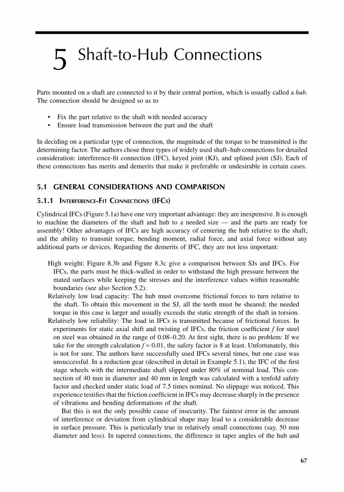
67
5
Shaft-to-Hub Connections
Parts mounted on a shaft are connected to it by their central portion, which is usually called a
hub
.The connection should be designed so as to
• Fix the part relative to the shaft with needed accuracy• Ensure load transmission between the part and the shaft
In deciding on a particular type of connection, the magnitude of the torque to be transmitted is thedetermining factor. The authors chose three types of widely used shaft–hub connections for detailedconsideration: interference-fit connection (IFC), keyed joint (KJ), and splined joint (SJ). Each ofthese connections has merits and demerits that make it preferable or undesirable in certain cases.
5.1 GENERAL CONSIDERATIONS AND COMPARISON
5.1.1 I
NTERFERENCE
-F
IT
C
ONNECTIONS
(IFC
S
)
Cylindrical IFCs (Figure 5.1a) have one very important advantage: they are inexpensive. It is enoughto machine the diameters of the shaft and hub to a needed size — and the parts are ready forassembly! Other advantages of IFCs are high accuracy of centering the hub relative to the shaft,and the ability to transmit torque, bending moment, radial force, and axial force without anyadditional parts or devices. Regarding the demerits of IFC, they are not less important:
High weight: Figure 8.3b and Figure 8.3c give a comparison between SJs and IFCs. ForIFCs, the parts must be thick-walled in order to withstand the high pressure between themated surfaces while keeping the stresses and the interference values within reasonableboundaries (see also Section 5.2).
Relatively low load capacity: The hub must overcome frictional forces to turn relative tothe shaft. To obtain this movement in the SJ, all the teeth must be sheared; the neededtorque in this case is larger and usually exceeds the static strength of the shaft in torsion.
Relatively low reliability: The load in IFCs is transmitted because of frictional forces. Inexperiments for static axial shift and twisting of IFCs, the friction coefficient
f
for steelon steel was obtained in the range of 0.08–0.20. At first sight, there is no problem: If wetake for the strength calculation
f
=
0.01, the safety factor is 8 at least. Unfortunately, thisis not for sure. The authors have successfully used IFCs several times, but one case wasunsuccessful. In a reduction gear (described in detail in Example 5.1), the IFC of the firststage wheels with the intermediate shaft slipped under 80% of nominal load. This con-nection of 40 mm in diameter and 40 mm in length was calculated with a tenfold safetyfactor and checked under static load of 7.5 times nominal. No slippage was noticed. Thisexperience testifies that the friction coefficient in IFCs may decrease sharply in the presenceof vibrations and bending deformations of the shaft.
But this is not the only possible cause of insecurity. The faintest error in the amountof interference or deviation from cylindrical shape may lead to a considerable decreasein surface pressure. This is particularly true in relatively small connections (say, 50 mmdiameter and less). In tapered connections, the difference in taper angles of the hub and
9563_C005.fm Page 67 Monday, August 6, 2007 4:21 PM

68
Machine Elements: Life and Design
the shaft presents an additional factor that reduces the load capacity. For these reasons,in important cases (for example, in lifting mechanisms of cranes), it is forbidden to useIFCs without key or other positive locking elements.
Detrimental effect on shaft strength: Elastic deformations under load result in local slippagein the connection and fretting damage of the mated surfaces (see Chapter 2, Section 2.2and Section 2.3). The fatigue strength of the shaft may be reduced by 70–80%. Withhigher-strength shaft materials, the detrimental effect of IFCs is greater.
Difficulty of dismantling: Assembly of an IFC is usually very easy: it is enough to warmup the hub or cool the shaft. However, dismantling may be problematic, particularly, whenthe mating surfaces are of low or middle hardness; there may be seizure and severe damageto the surfaces.
During continuous duty, the condition of the mating surfaces changes (because of the microslippagementioned previously), and the friction coefficient increases owing to seizure and fretting. Sometimes,pressing out of this connection is impossible and one of the parts must be cut to save the other.
Radical facilitation of dismantling is achieved by using a tapered IFC, which allows hydraulicdismantling (Figure 5.1b). The angle of the taper in this case is usually chosen between 1
°
54
′
35
′′
(taper 1:30) and 1
°
08
′
45
′′
(1:50). Oil is pumped through inlet 1 to spiral grooves 2 under highpressure that must exceed the surface pressure in the connection (the pressure may be in hundredsor even thousands of bar). When this oil pressure separates the hub from the shaft, the frictioncoefficient becomes very low, and the hub rushes off the shaft with a high speed. To prevent injuryto personnel and damage to the parts, safe stoppers must be installed before dismantling. In thedesign shown in Figure 5.1b, nut 3 slackened by several millimeters may be an ideal stopper.
Tapered connections are more expensive, because machining the tapered surfaces is quitedifficult when interchangeability is needed. The next step toward simpler production is separationof the tapered part, and manufacturing a unit at a specialized works equipped for this task. Figure 5.2ashows a rigid coupling for joining two coaxial shafts of the same diameter. Thin-walled sleeve 1has a cylindrical inner surface and a tapered outer surface. An interference fit is achieved by theaxial movement of heavy-walled shell 2. High-pressure oil is led through inlet 3 to spiral grooves
FIGURE 5.1
Interference-fit connections.
1
(a) (b)
3
2
9563_C005.fm Page 68 Monday, August 6, 2007 4:21 PM

Shaft-to-Hub Connections
69
4 (to separate the sliding tapered surfaces), and the shell is moved relative to the sleeve by bolts5 nested in nut 6. (After assembly, bolts 5 must be removed, but the locked nut remains in place.)The contact pressure in the joint is determined indirectly by measuring the increase in the outerdiameter of the shell. To dismantle the coupling, the high-pressure oil is led through inlet 3 tospiral grooves 4, and as the oil film separates shell 2 from sleeve 1, the shell gets off the sleeve,and nut 6 serves as a stopper.
Figure 5.2b shows the connection of flange 7 with a shaft by means of radial deformation of theflange hub. The needed surface pressure is created when discs 8 clamped by bolts 9 squeeze double-tapered split sleeve 10, which in turn squeezes the hub of flange 7 and presses it against the shaft.The tapered surfaces of parts 8 and 10 as well as bolts 9 should be coated with MoS
2
grease todecrease the coefficient of friction in these places. That increases the radial squeezing forces thatclamp the coupling and facilitates the cone’s disengagement while releasing. Mating surfaces of theflange and the shaft should be degreased so as to increase the friction and the load capacity of the IFC.
Another version of such a coupling that attaches a pulley to a shaft is shown in Figure 5.2c.Double-tapered split sleeves 11 and 12 are deformed in the radial direction by means of double-tapered rings 13 and 14 pulled together by bolts 15. In this case, the contacting surfaces of theinner sleeve with the shaft and the outer sleeve with the pulley should be degreased.
The couplings depicted in Figure 5.2 represent versions of IFCs, and all the demerits of IFCsare valid for them, with the exception of “difficulty of dismantling.” In some cases, the slippageof IFCs can be considered as a merit: in case of overload, it may play the role of a torque limiterand protect the mechanism from damage. Nevertheless, it is undesirable to use an IFC as a torquelimiter for three reasons. First, if you need a torque limiter, it is preferable to use a special device,which enables more exact setting of the maximal torque. Second, the IFC becomes less reliableafter slippage because the mating surfaces are subjected to wear, and the coefficient of frictiondecreases as well. To be on the safe side, the coupling should be dismantled and inspected afterthe slippage, because the coupling and the shaft may not only be worn out but also overheated,scratched, and possibly cracked. And third, you never know whether there was a slippage in theconnection or not, so the reliability of the machine is permanently questionable. Therefore the loadcapacity of the IFC must be several times greater than the transmitted load to safely prevent slippage.
5.1.2 K
EY
J
OINTS
(F
IGURE
5.3)
Usually, a KJ is an IFC with the addition of a key that prevents slippage during the transmissionof a torque. The KJ is somewhat more expensive than IFC because the keyways must be machinedin the hub and on the shaft journal. But KJ is much more reliable and capable of transmitting torque.
In principle, the KJ is also able to transmit a torque when the hub is slide-fitted to the shaft,but the durability of the connection decreases sharply. The permissible load in this case is very
FIGURE 5.2
Easily disassembled interference-fit connections.
(a) (b) (c)
1235 6
4
10
78 9 14 11
13
12
15
9563_C005.fm Page 69 Monday, August 6, 2007 4:21 PM

70
Machine Elements: Life and Design
low, and the key is usually screwed to the shaft to prevent its turning (see Figure 5.10d). When theshaft is rotating, the hub moves cyclically relative to the key and the shaft within the radial clearance,causing wear. Lubrication of such connections is a must.
The aforementioned demerits of IFCs (with the exception of “relatively low load capacity andreliability”) are valid for KJs as well. The detrimental effect on the shaft strength is even strongerbecause the shaft is additionally weakened by the keyway. But the combination of high reliabilityand load capacity with a moderate cost has motivated the widespread use of KJ in machineryconstruction, where there is no tight limitation on weight and the needed shaft strength may beachieved by increasing its diameter.
5.1.3 S
PLINED
J
OINTS
(SJ
S
) (F
IGURE
5.4)
Merits of the SJ:
Highest load capacity when transmitting a torque: As was already said, the static strengthof the SJ in torsion is more than that of the shaft. This torsional strength is provided atthe moderate joint length required for wear resistance.
FIGURE 5.3
Key joints.
FIGURE 5.4
Splined joints.
(a) (b)
Shaft
Hub
9563_C005.fm Page 70 Monday, August 6, 2007 4:21 PM

Shaft-to-Hub Connections
71
Least weight of parts: The thickness of the hub and shaft is dictated by the needed strengthfor transmission of the load; therefore, the parts may be thin walled (tubular) and relativelylightweight.
Capability of working with clearances and misalignments: These abilities enable an effectiveuse of the SJ for axially shifted parts (for example, for shifting gears in gear boxes). It isalso used to compensate misalignment in the connection of two coaxial shafts. Such SJsshould be generously lubricated for long-term usage.
Lesser detrimental effect on shaft strength (as compared with IFCs and KJs): Strength decreasein the SJ is caused by geometric stress raisers. Their influence is quite predictable, and it isconsiderably less than the influence of the stress concentration and fretting in IFCs and KJs.
In SJs, fretting occurs rarely because they are lubricated. But even if fretting occurs, it islimited to the contact surfaces of the teeth, at a certain distance from the most stressedplaces (which are the tooth fillets) and doesn’t affect shaft strength.
Easy assembly and dismantling: SJ is usually designed with a sliding fit, so there is noproblem with assembly and dismantling. When the SJ must be tightly fitted, temperaturedeformation is used for easy assembly.
If there were no demerits in SJs, they would be used everywhere, and we would not be evenaware of the other types of the hub–shaft connections. But, fortunately, they have demerits as well:
Relatively high cost: In some cases it is not just expensive but completely impossible tomachine splines into the hub or on the shaft because they are too large for the availablegear-cutting or broaching machines.
Lower precision of centering the hub relative to the shaft: The simpler the geometry of themating surfaces, the more precise the machining can be. In IFC and KJ, these surfaces arejust cylinders or tapers, and these connections are gapless, so they ensure the best centeringprecision. In an SJ the spline surfaces are complicated, and machining is less accurate. Ifhigh accuracy of centering in the radial direction is needed, auxiliary surfaces — cylindricalor conical — are usually used (see Section 5.4), and that complicates the design.
The areas of application of these connection types may be determined from the features statedpreviously. Where maximal reliability, minimal weight, or both are required (for example, in aviationand automotive engineering), SJs are usually used. In general engineering, where dimensions andweight are not so restricted, KJs (with a press fit) are prevalent.
The difficulty of dismantling IFCs and KJs doesn’t confuse the designer if, in regular serviceconditions, the connection will not be dismantled. In case of damage, the damaged part may be cut,easily separated from the usable one, and replaced. For example, if the teeth of a gear have beenbroken, the gear may be cut in radial direction in the area of the keyway to release the surfacepressure in the connection. After that, the shaft can be pressed out of the gear, inspected for possiblesurface damages and fatigue cracks, and then reused if everything is OK.
The IFC (without a key) is used when the torque and the axial force are low relative to thedimensions of the connection, for example, in the connection of railroad car wheels with theiraxles, the rotor of an electric motor with the shaft, etc. Use of IFCs for transmission of high loadsis recommended only on condition that it will be thoroughly tested before being placed in service.
5.2 STRENGTH CALCULATIONS AND DESIGN OF IFCs
5.2.1 C
ALCULATION
FOR
T
OTAL
S
LIPPAGE
An IFC transmits load by means of friction. The area of the joint surface is
A dl mm= π 2
9563_C005.fm Page 71 Monday, August 6, 2007 4:21 PM

72
Machine Elements: Life and Design
and the total friction force is
(5.1)
where
d
and
l
are the diameter and length of the connection (mm)
p
=
surface pressure (MPa)
f
=
coefficient of friction
Equation 5.1 looks extremely logical and easy. The problem is that only the
d
and
l
values areknown exactly, because these are specified by the designer and they can be measured. Concerningthe pressure
p
and, particularly, the friction coefficient
f
, the designer is forced to proceed fromassumptions and information that may not correspond with reality. But let’s consider these twofactors in more detail.
5.2.1.1 Surface Pressure
To determine the surface pressure
p
, the Lame equation (1833) is used. That equation is truefor infinitely long and perfectly precise round cylinders, but it is successfully used for real partswith small corrections. The need of corrections arose from the fact that the contact betweenthe hub and shaft takes place not over the entire surface uniformly but first in spots; this isbecause the parts have surface roughness and waviness, out-of-roundness, and other deviationsfrom the ideal shape. Therefore, the compliance of the parts increases (see the roughness-dependent second member of Equation 6.7 in Chapter 6, Subsection 6.2.5). As the interferencegrows, the entire surface of the joint comes into contact, and in the spots of initial contact,there may be plastic deformation of the surface layer. Because of this, the influence of thesurface deviations is limited. At the relatively high pressures typical of IFCs, it is usually takeninto account by reducing the rated radial interference by 60% of the sum of the roughnessheights of the mating surfaces
R
z
.If the joint diameter is
d
, the diameter of the central hole in the shaft is
d
1
and the outer diameterof the hub is
d
2
(Figure 5.5), the surface pressure for materials with the same modulus of elasticity
E
may be determined from this equation:
where
E
=
modulus of elasticity (MPa) of the hub and the shaft (If the hub and the shaft have different moduli of elasticity, another equation, more complicated, should be used.)
d
1
and
d
2
=
diameters (mm)
δ
=
rated interference ( mm) determined from the equation
where
d
S
and
d
H
=
measured joint diameter of the shaft and the hub
R
ZS
and
R
ZH
=
roughness heights of these surfaces (all in mm)
F dl p f Nf = π
pEd
d d d d
d d=
−( ) −( )−( )
δ2 3
212
22 2
22
12
MPa
δ = − − +( ) . ( )d d R RS H ZS ZH1 2
9563_C005.fm Page 72 Monday, August 6, 2007 4:21 PM

Shaft-to-Hub Connections
73
If there is no central hole in the shaft (
d
1
=
0), then the equation for the surface pressurebecomes simpler:
(5.2)
The diameters that appear in these equations may be variable. In such cases, the designers usuallysimplify the problem. For example, in tapered connections the diameter
d
may be taken as anaverage of the minimal and maximal values. The outer surface represented by diameter
d
2
mayhave a flange (as in Figure 5.5) or another stiffener, which increases the surface pressure in thevicinity. Usually these changes in
d
2
are neglected. A more precise calculation may be performedusing finite element method (FEM).
For tapered IFCs, the equality of the taper angles of the shaft and the hub is very importantbecause it directly influences the amount of interference. Apparently, the maximal divergence ofthe cones should not exceed 10–15% of the rated interference. The needed interference is achievedby an axial movement of the hub relative to the shaft from the initial position, in which they arepressed against each other with a relatively small force. It is preferable to have the initial contactin the area of the larger diameter of the connection, because there the transmitted torque is maximal.
The real surface pressure may be controlled after assembly by measuring the increase of theouter diameter of the hub (
∆
). The increase of the outer diameter for a cylindrical hub may bederived from a formula:
When
E
and
p
are expressed in MPa,
d
and
d
2
are in mm, and so is
∆
as well.If the parts are made of materials with different moduli of elasticity and Poisson’s ratio, the
formula is somewhat more complicated, and can be found in handbooks.
FIGURE 5.5
Interference-fit main dimensions.
l
d1 dd2
pEdd
d d= −( )δ2 2
2 22 2
∆ =−( )
d d p
E d d
22
22 2
9563_C005.fm Page 73 Monday, August 6, 2007 4:21 PM

74
Machine Elements: Life and Design
The calculation of the IFC should take into account the possible differences in temperatureduring manufacture, storage, and service. During manufacture, the temperature is about 20
°
C;during storage and use, it may change in the range from, say,
−
60 to
+
100
°
C. If, for example, analuminum part is mounted with an interference fit on a steel shaft at a temperature of
+
20
°
C, theinterference will increase by about 0.09 mm for each 100 mm of the joint diameter at
−
60
°
C. Thismay cause some plastic deformation (depending on the initial surface pressure) and reduce theinterference. If, in service, the temperature is
+
100
°
C, the interference decreases additionally by0.09 mm for each 100 mm of the joint diameter, and impairs the load capacity of the IFC.
Considerable decrease in interference while in operation may be caused by centrifugal forces.At high rotational speed, the joint may be completely separated, and this may lead not only toslackening of the connection, but also to imbalance of the rotor and increased vibrations. The onlyremedy for this is to increase the initial interference so as to ensure the needed tightness at maximalworking speed.
5.2.1.2 Coefficient of Friction
When the hub is turned or moved in the axial direction relative to the shaft, the force first comesto a maximum (static friction coefficient
f
S
), and then, it decreases to the amount which conformsto the sliding friction coefficient
f
(Figure 5.6).According to experiments,
For calculation, it may seem reasonable to use the maximal coefficient of friction
f
S
, and it is correctwhen even a small slippage in the connection is inadmissible (for example, in kinematical trans-missions). In many cases, a single small slippage on a momentary overload is not dangerous.However, if the connection is once broken, the repeated slippage occurs at a lesser load, nearlyconforming to the sliding coefficient of friction
f
(peaks 1 in Figure 5.6). Therefore, as a rule, the
f
value is used in calculations for total slippage. The values of
f
for steel parts in experiments rangefrom 0.08 to 0.18 when assembled by applying an axial force (pressing). When assembled usingradial deformation of parts (heating the hub, cooling the shaft, or causing deformation usinghydraulic pressure or intermediate tapered parts), the range is from 0.12 to 0.20. It is reasonablethat the minimal values should be taken for calculations:
f
= 0.08 for assembly by force and f = 0.12when radial deformation is used. These values are valid for a static loading without any vibrationsor cyclic bending. At these conditions, the axial force that the IFC is able to transmit is equal to
FIGURE 5.6 Torque vs. rotating angle while breaking interference fit.
f to fS ≈ ( . )1 5 2
T
ϕ
1
T(f )
T(fs)
9563_C005.fm Page 74 Monday, August 6, 2007 4:21 PM

Shaft-to-Hub Connections 75
the friction force Ff and is determined by Equation 5.1. Regarding the torque, it is equal to theproduct of Ff and d/2:
(5.3)
Experiments show that during cyclic bending of the shaft, the slip resistance of IFC decreases.The reason for this is that the bending is accompanied by a local microslippage, and in theseareas, the friction coefficient decreases almost to zero. In addition, if the bending stress on oneside of the connection is larger than on the other side, there arises an axial force aimed to pressthe shaft out of the hub toward the larger bending stress. (See Chapter 2, Section 2.1.)
According to experimental data,1 when the IFC is loaded with an axial force or a torque, andthe shaft is simultaneously loaded with a cyclic bending moment, the dynamic coefficient of frictionfdyn may be obtained from the formula
(5.4)
wheref = static coefficient of frictionσa = bending stress amplitudep = surface pressure in the connectiond and l = diameter and length of the connectionβ = 0.08 ± 0.008 is an experimentally determined factor
It was noticed that the mean bending stress doesn’t influence the load capacity of the IFC. Onlythe amplitude σa affects it.
When the bending stress becomes so large that fdyn = 0, the hub begins moving relative to theshaft (in the axial direction) without any external force. If the value of fdyn obtained from Equation 5.4is negative, some form of stopper must be used to prevent the self-dismantling of the connection.
Equation 5.4 is valid when the bending stress on one side of the connection is zero. If thereare bending stresses on both sides, the experiments mentioned previously give the following relation:
(5.5)
In this formula, σa1 is the larger bending stress, and σa2 is the lesser bending stress (on theother side of the IFC); β1 = 0.08 and β2 = 0.05.
It was noted that if the external force (load) tended to move the hub relative to the shaft in adirection opposite to the direction of self-dismantling, then β1 = β2 = 0.05.
The substitution of σ2 = 0 into Equation 5.5 transforms it into Equation 5.4. As is seen from theseequations, the longer the connection, the less the influence of bending on the load capacity of the IFC.
In contrast to the transmission of axial forces, the torque transmitting capacity never decreasesto zero, but it may be as little as 15% or less of the static load capacity. The data cited previouslyis based on extensive experiments with IFCs of 30, 70, and 160 mm in diameter and with d/lranging from 0.1 to 1.5.1
EXAMPLE 5.1
Let’s analyze the case of IFC slippage mentioned in the beginning of Section 5.1 regarding“relatively low reliability.” The case in point is the intermediate shaft of a double-reduction gear
Td l p f
N mmf = ⋅π 2
2
f fp
dldyn
a= − βσ
f fp
dldyn
a a a= − − +β σ σ β σ1 1 2 2 2( )
9563_C005.fm Page 75 Monday, August 6, 2007 4:21 PM

76 Machine Elements: Life and Design
shown in Figure 5.7a (sketch of a gear) and Figure 5.7b (the shaft to be investigated). The centerdistance of the input stage C1 = 115 mm, gear ratio i1 = 5, so the gear diameter D1 = 191.7 mm.The output stage center distance C2 = 160 mm, i2 = 5, so the pinion diameter d2 = 53.3 mm. Theoutput torque of the gear is 2000 N⋅m, so at the intermediate shaft, each gear transmits a nominaltorque of 200 N⋅m to the pinion. The IFC strength calculation was performed without taking intoaccount dynamic factors and unevenness of load distribution between the gears of the input stage,but the safety factor was taken as k = 10. The needed surface pressure was found from Equation 5.3:
(5.6)
Substitution of Tf = 2⋅105 N⋅mm, d = l = 40 mm, f = 0.12, and k = 10 gives p = 165.8 MPa. Themanufacturing tolerances of the shaft and gears were chosen so as to ensure this pressure at minimalinterference.
Now it is time to do a more accurate calculation of the IFC of the gear to the pinion shaft.First, consider the possibility that the load distribution may be uneven between the two halves ofthe “herringbone.” The helix angle of the gear teeth is ψ = 30°, and for this angle the load factoris KWh = 1.32 (see Chapter 7, Figure 7.22). The dynamic factor may be approximately taken asKd = 1.35. Hence, the total torque transmitted by one gear equals
(Admittedly, there is some exaggeration in such use of the dynamic factor Kd. The dynamic loadhas been mostly taken by the mass of the gear, and only part of it results in increased torque.But we try to find out the reasons for the IFC slippage; so we take the maximum possibleoverload.)
A calculation of the bending stresses in the pinion shaft gives the following: in section 1,σ1 = 121.2 MPa; in section 2, σ2 = 29.2 MPa. From Equation 5.5, the coefficient of friction equals
FIGURE 5.7 Intermediate shaft of a double-reduction gear.
1
2
(a) (b)
85
115
160
23
2
40
d2 D1 ∅40
∅65
pT
d l fkf=
22π
T Nm= ⋅ ⋅ =200 1 32 1 35 356 4. . .
fdyn = − − + ⋅ =0 120 08 121 2 29 2 0 05 29 2
165 80.
. ( . . ) . ..
..067
9563_C005.fm Page 76 Monday, August 6, 2007 4:21 PM

Shaft-to-Hub Connections 77
Thus, we see that owing to the bending stresses, the coefficient of friction may degrade to almosthalf of its static value. But it doesn’t explain the observed slippage of the IFC. To transmit the354.6 N⋅m torque, it is enough to have coefficient of friction (from Equation 5.3)
So, the obtained coefficient of friction fdyn = 0.067 is enough to transmit even threefold torque.But because there was a slippage, the real coefficient of friction was less than 0.021. Consequently,our calculation was based on wrong assumptions about the f value. Taking into consideration thatthe connection has passed the static test under 7.5-fold load, an additional reduction in the coefficientof friction owing to vibrations should be supposed. In experiments with bolt connections, a reductionin the coefficient of friction (because of vibrations) from 0.13–0.14 to 0.01, and even to 0.005, wasnoticed. Obviously, this was the second cause of the slippage; low accuracy of the gears set upvibrations, and the friction in the IFC became too low.
When IFCs are not exposed to heavy vibrations and bending loads, the rated safety factor k = 3is usually considered as sufficient (once again, when the possible slippage is not dangerous).
5.2.2 DESIGN OF IFCS
Every design begins with something known; in this case, it is the approximate diameter d (reasoningfrom the diameter of the shaft) and load to be transmitted. The designer chooses the length of theconnection (usually l = (1–1.5)d), the coefficient of friction f, and the safety factor k. This is enoughto determine the needed surface pressure p, the needed amount of interference, and then the stressesthat the IFC induces within the parts.
The maximal stresses take place on the joint surfaces. On the shaft,
(5.7)
and on the joint surface of the hub,
(5.8)
These stresses are constant and they should not, under any circumstances (such as change oftemperature, influence of load and other), exceed the yield point Sy of the material, otherwise thereal interference and surface pressure may become less than the rated ones. So,
These stresses should be calculated for the minimal rated value of p. The sufficient safety factorin this case is 1, because if there is a plastic deformation, the surface pressure decreases automat-ically to the admissible value, and the plastic deformation ceases.
The sum of the radial deformations of the hub (outward) and the shaft (inward) represents theinterference value δ that is needed to achieve the required surface pressure p. The larger theinterference, the less the influence of manufacturing tolerances on the load capacity of IFC. Buton the other hand, the large interference may cause problems when assembling.
fT
d lp= = ⋅
⋅ ⋅ ⋅=2 2 354600
40 40 165 80 021
2 2π π ..
τmaxS p
dd d
=−12
212
τmaxH p
dd d
=−
22
22 2
τmax .≤ 0 5Sy
9563_C005.fm Page 77 Monday, August 6, 2007 4:21 PM

78 Machine Elements: Life and Design
EXAMPLE 5.2
A shaft transmits torque of T = 10 kN⋅m. On its end is attached a flange by means of IFC. Thebending moment is negligible. The tensile strength of the shaft material is Su = 950 MPa. Roughnessheight of the mating surfaces Rz = 10 mkm.
The diameter of the shaft may be approximately obtained from Equation 4.1 because the shafthas a sharp stress raiser (an IFC):
We take d = 110 mm, and the length of the connection l = 150 mm. Assuming f = 0.12 and thesafety factor k = 3, the required surface pressure p derived from Equation 5.6 is
First, take the shaft without a central hole (d1 = 0) and the outer diameter of the hub d2 = 1.6d ≈175 mm. Now, let’s determine the deformations of the hub and the shaft under this pressure. Increaseof the hub inner diameter is
Decrease of the shaft outer diameter is
To determine the required value of the interference δ, we should sum up the deformations of thehub and the shaft and add 60% of the total roughness height:
This value of interference should be considered as minimal. Taking into account the tolerance ofthe shaft neck (0.022 mm) and that of the hub inner diameter (0.035 mm), the maximal interferencein this connection will be 0.179 + 0.022 + 0.035 = 0.236 mm.
To ensure some assembly clearance by heating the hub, the radial deformation caused by heatingshould be at least 0.3 mm. Considering the linear expansion factor of steel α = 12 ⋅ 10−6 1/°C, therequired difference between the temperatures of the hub and the shaft is
That means that if the shaft temperature is 20°C, the hub should be heated to 250–270°C. Ifthe shaft is chilled in liquid nitrogen to −70°C, the hub needs be heated only to 160–180°C.
d ≈ ⋅ ⋅ =( )5 610000 10
950109 130
33to to mm
p = ⋅ ⋅ ⋅⋅ ⋅ ⋅
=2 10000 10 3110 150 0 12
87 73
2π .. MPa
∆ddpE
d dd dH = +
−+
= ⋅⋅
222
22 2
110 87 72 06 10
µ .. 55
2 2
2 2
110 175175 110
0 3 0 122+−
+
=. . mm
∆ddpE
d dd dS = +
−−
= ⋅⋅
212
212
110 87 72 06 10
µ .. 55
1 0 3 0 033( . ) .− = mm
δ = + + + = + +∆ ∆d d R RH S Z Z1 2 0 122 0 033 1 2 0 011 2. ( ) . . . ( . ++ =0 01 0 179. ) . mm
∆td
=⋅
=⋅ ⋅
=−
δα
0 3110 12 10
2276
. C
9563_C005.fm Page 78 Monday, August 6, 2007 4:21 PM

Shaft-to-Hub Connections 79
Let’s calculate this connection with thin-walled parts. Say, the shaft has a central hole d1 = 70mm, and the outer diameter of the hub d2 = 140 mm. Because the torque transmitted is the same,the required surface pressure is also the same. In this case, the changes in the diameters of the huband of the shaft are as follows:
The minimal interference (the difference of the diameter d values measured on the shaft neck andinside the hub) is
Taking into account the manufacturing tolerances, the maximal interference may be as large as0.333 + 0.022 + 0.035 = 0.390 mm. For sufficient radial deformation (by about 0.45 mm) usingheating or chilling, the difference in temperatures of the hub and shaft should be about 340°C.
Now it is worth checking the stresses in the parts caused by the interference fit. As mentioned,we check it at a minimal required surface pressure. Using Equation 5.7 and Equation 5.8, we obtainthe maximal shear stresses in the shaft and the hub:
The stress in the hub is quite big, and so the material should have a yield point of at least 500 MPa.The design of IFCs is extremely simple. Measures to diminish the detrimental effect of this
connection on the fatigue strength of the shaft have been discussed in Chapter 4, Section 4.2.
5.3 DESIGN AND STRENGTH CALCULATION OF KEY JOINTS
5.3.1 ROLE OF THE IFC IN THE KEY JOINT
The main condition that should be met to ensure durable serviceability of KJ is a complete (as far aspossible) prevention of any relative movement in the connection. This is achieved by prestressing thejoint using an IFC, and the friction force should transmit the entire torque with a safety factor of 1.3 to 1.5.
The needed prestressing may be made also by taper keys or tangent keys, but they move thehub in radial direction relative to the shaft, causing a certain radial runout of the hub. Therefore,such connections are used rarely, usually for low-speed shafts, and when a high accuracy is notrequired. But they are not discussed here.
In connections with a large taper (say, 1:10, where the angle of the taper is numerically largerthan the coefficient of friction), the needed prestress can’t be achieved by just assembly, becausethe hub will slip off the shaft. There must be an axial tightening using a nut or an end plate(Figure 5.8). The needed tightening force is obtained from the equation
(5.9)
∆dH = ⋅⋅
+−
+110 87 7
2 06 10110 140140 110
0 35
2 2
2 2
..
.
=
= ⋅⋅
+
0 212
110 87 72 06 10
110 7015
2 2
.
..
mm
∆dS 110 700 3 0 097
2 2−−
=. . mm
δ = + + + =0 212 0 097 1 2 0 01 0 01 0 333. . . ( . . ) . mm
τ
τ
max
max
. .
.
S
H
=−
=
=
87 770
110 7059 7
87 7140
2
2 2
2
MPa
1140 110229 2
2 2−= . MPa
FT f
d fk Ntight
m
= +2 (sin cos )α α
9563_C005.fm Page 79 Monday, August 6, 2007 4:21 PM
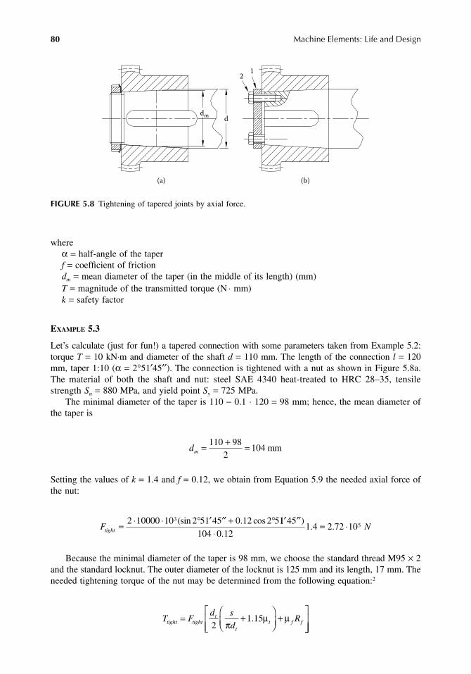
80 Machine Elements: Life and Design
whereα = half-angle of the taperf = coefficient of frictiondm = mean diameter of the taper (in the middle of its length) (mm)T = magnitude of the transmitted torque (N ⋅ mm)k = safety factor
EXAMPLE 5.3
Let’s calculate (just for fun!) a tapered connection with some parameters taken from Example 5.2:torque T = 10 kN⋅m and diameter of the shaft d = 110 mm. The length of the connection l = 120mm, taper 1:10 (α = 2°51′45′′). The connection is tightened with a nut as shown in Figure 5.8a.The material of both the shaft and nut: steel SAE 4340 heat-treated to HRC 28–35, tensilestrength Su = 880 MPa, and yield point Sy = 725 MPa.
The minimal diameter of the taper is 110 − 0.1 ⋅ 120 = 98 mm; hence, the mean diameter ofthe taper is
Setting the values of k = 1.4 and f = 0.12, we obtain from Equation 5.9 the needed axial force ofthe nut:
Because the minimal diameter of the taper is 98 mm, we choose the standard thread M95 × 2and the standard locknut. The outer diameter of the locknut is 125 mm and its length, 17 mm. Theneeded tightening torque of the nut may be determined from the following equation:2
FIGURE 5.8 Tightening of tapered joints by axial force.
dm
(a) (b)
12
d
dm = + =110 982
104 mm
Ftight = ⋅ ⋅ ° ′ ′′ + ° ′2 10000 10 2 51 45 0 12 2 53(sin . cos 11 45104 0 12
1 4 2 72 105′′
⋅= ⋅)
.. . N
T Fd s
dRtight tight
t
tt f f= +
+
2
1 15π
µ µ.
9563_C005.fm Page 80 Monday, August 6, 2007 4:21 PM

Shaft-to-Hub Connections 81
wheres = thread pitch (here s = 2 mm)dt = thread diameter (dt = 95 mm)µt and µf = coefficients of friction in the thread and between the hub and the face
of the nut, correspondingly (we take µt = µf = 0.14)Rf = average radius of the nut face (Rf = 52 mm)
Inserting these values into the preceding formula gives us the nominal tightening torque:
When tightening is performed using a manual torque wrench or precision screwdriver, thepossible deviation of the tightening force from its calculated value may be about ±23% (accordingto the Bossard estimation3). It depends on friction fluctuations. Hence, to ensure the needed axialforce at a higher friction, the tightening torque should be increased by 23%:
But at a lower friction, the axial force may be greater than needed by 23% because of lesser frictionand by another 23% because of increased tightening torque. That means,
What do you think about this force? Imagine, it is 40 tons! Surely, the shaft and the nut shouldbe checked for strength. The inner diameter of the thread is about 92 mm, so the diameter of thecircular groove between the thread and the tapered part of the shaft may be equal to 90 mm. Thearea of this section A and the tension stress σ are as follows:
No problem. What about the thread strength? It looks too weak for the huge axial load. Theshear stress in the thread can be determined from the formula2
wheredi = inner diameter of the thread (di ≈ d − 1.3p = 95 − 1.3⋅2 = 92.4 mm)h = engaged length of the thread (h = 17 mm)k = coefficient that takes into account the thread vees (k = 0.87 for triangular thread)
Ttight nom, . . .= ⋅⋅
+ ⋅
2 72 10952
295
1 15 0 145
π++ ⋅
= ⋅ ⋅0 14 52 4 147 106. . N mm
T N mmtight = ⋅ ⋅ = ⋅ ⋅4 147 10 1 23 5 1 106 6. . .
F Ntight ,max . . .= ⋅ ⋅ = ⋅2 72 10 1 23 4 12 105 2 5
A = ⋅ = = ⋅ =π σ904
63624 12 10
636264 8
22
5
mm MPa;.
.
τπ
=F
d hktight
i
,max
τπ
= ⋅⋅ ⋅ ⋅
=4 12 1092 4 17 0 87
965.
. .MPa
9563_C005.fm Page 81 Monday, August 6, 2007 4:21 PM

82 Machine Elements: Life and Design
The yield stress in shear
Thus, the safety factor for shear strength equals 435/96 = 4.5.Let’s calculate the strength of the nut. It looks like a ring; Figure 5.9 shows (a) the radial forces
in the threads and (b) axial forces evenly distributed over the circumference. Because the axialforces and contraforces are distanced in the radial direction (C, Figure 5.9b), the ring is loaded bya shear force, which is equal to Ftight, max, and a twisting moment. Both the shear force and twistingmoment are evenly distributed over the circumference. Now, as we have analyzed the kinds ofloading forces, we are ready to calculate the stresses.
The mean diameter of the thread dmt = 93.7 mm, and the unit axial force is
The angle of the thread profile is 60°, so the unit radial force in the thread equals
The tension stress in the ring caused by these radial forces is (approximately)
Here, Ar is the area of the ring section. The dimensions of the nut are as follows: in the axialdirection it measures 17 mm, and in the radial direction, 11 mm (from the outer diameter of the
FIGURE 5.9 Sketch to strength calculations.
τ y yS≈ = ⋅ =0 6 0 6 725 435. . MPa
qF
dN mm
a
tight
mt
=⋅
= ⋅⋅
=,max ..
/π π
4 12 1093 7
14005
q q N mmr a= ° = ⋅ =tan . /30 1400 0 5773 808
σ1 2= q d
Ar mt
r
(a)
h
b
(b) (c)
h1
F
F
dmt
b1
a1Rf
c
9563_C005.fm Page 82 Monday, August 6, 2007 4:21 PM
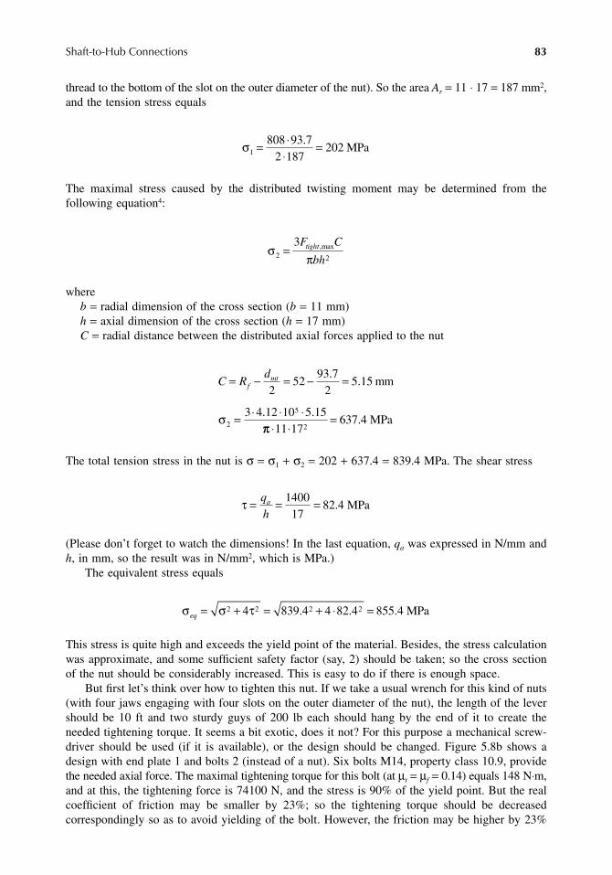
Shaft-to-Hub Connections 83
thread to the bottom of the slot on the outer diameter of the nut). So the area Ar = 11 ⋅ 17 = 187 mm2,and the tension stress equals
The maximal stress caused by the distributed twisting moment may be determined from thefollowing equation4:
whereb = radial dimension of the cross section (b = 11 mm)h = axial dimension of the cross section (h = 17 mm)C = radial distance between the distributed axial forces applied to the nut
The total tension stress in the nut is σ = σ1 + σ2 = 202 + 637.4 = 839.4 MPa. The shear stress
(Please don’t forget to watch the dimensions! In the last equation, qa was expressed in N/mm andh, in mm, so the result was in N/mm2, which is MPa.)
The equivalent stress equals
This stress is quite high and exceeds the yield point of the material. Besides, the stress calculationwas approximate, and some sufficient safety factor (say, 2) should be taken; so the cross sectionof the nut should be considerably increased. This is easy to do if there is enough space.
But first let’s think over how to tighten this nut. If we take a usual wrench for this kind of nuts(with four jaws engaging with four slots on the outer diameter of the nut), the length of the levershould be 10 ft and two sturdy guys of 200 lb each should hang by the end of it to create theneeded tightening torque. It seems a bit exotic, does it not? For this purpose a mechanical screw-driver should be used (if it is available), or the design should be changed. Figure 5.8b shows adesign with end plate 1 and bolts 2 (instead of a nut). Six bolts M14, property class 10.9, providethe needed axial force. The maximal tightening torque for this bolt (at µt = µf = 0.14) equals 148 N⋅m,and at this, the tightening force is 74100 N, and the stress is 90% of the yield point. But the realcoefficient of friction may be smaller by 23%; so the tightening torque should be decreasedcorrespondingly so as to avoid yielding of the bolt. However, the friction may be higher by 23%
σ1
808 93 72 187
202= ⋅⋅
=.MPa
σπ2 2
3=
F C
bhtight ,max
C Rd
fmt= − = − =
= ⋅ ⋅ ⋅
252
93 72
5 15
3 4 12 10 5 152
5
..
. .
mm
σππ ⋅ ⋅
=11 17
637 42
. MPa
τ = = =q
ha 1400
1782 4. MPa
σ σ τeq = + = + ⋅ =2 2 2 24 839 4 4 82 4 855 4. . . MPa
9563_C005.fm Page 83 Monday, August 6, 2007 4:21 PM

84 Machine Elements: Life and Design
as well, and the tightening force (already decreased by 23% because of decreased tightening torque)will decrease additionally. So the minimal tightening force is
The total minimal tightening force is 48980 x 6 = 2.94 ⋅ 105 N, and this is rather more than weneed (2.72 ⋅ 105 N).
The end plate should be checked for strength and rigidity under a maximal tightening force(74100 N on each bolt). For the approximate calculation, the end plate may be represented as around plate simply supported around the periphery. It is loaded by an axial force F evenly distributedover the circumference passing through the centers of the bolts (b1 = 38 mm, Figure 5.9c). To beginwith, let’s take the thickness of the plate to be about equal to the bolt diameter: h1 = 15 mm.
The evenly distributed bending moment in the plate at a radius b1 is determined by the formula5
where F = 74100 x 6 = 4.45 ⋅ 105 N, a1 = 52 mm, b1 = 38 mm, and ν = 0.3; thus,
The bending stress in the plate equals
Now we should take into account that the real end plate has holes for the bolts on this diameter.Six holes of 15 mm diameter take 37.7% of the circumference of the bolt circle of 38 mm radius.Hence, the real length of the plate section that takes the bending moment is only 62.3% of thecircumference. Thus, the calculated stress in the real plate equals 538.6/0.623 = 864.4 MPa. Thisstress is too high. If we made the plate from a high-strength steel with the yield point of 900 MPaand take a safety factor of 1.5 (considering that our calculation is approximate), the admissiblecalculated stress is 600 MPa. The stress is related inversely to the square of the plate thickness h1;so the needed thickness should be
Approximating to the nearest standard thickness of the rolled plate, we choose 20 mm.The end plate bends elastically under load, and there will be some angle between the plate and
the bearing surface of the bolt head. Angular deflection of the plate surface at the radius b1 isdetermined as follows:5
F Ntight ,min .= =74100
1 2348980
2
MF a b
aba
=− −( )
− +
4
1
211
212
12
1
1πν
ν( )
( ) ln
M = ⋅ − −⋅
− +4 45 104
1 0 3 52 382 52
1 0 35 2 2
2
. ( . )( )( . ) ln
π33852
2 02 104
= ⋅ ⋅. /N mm mm
σ = = ⋅ ⋅ =6 6 2 02 1015
538 612
4
2
Mh
.. MPa
h1 15864 4600
18= ⋅ =mm mm.
Θ =+( )
=−
= ⋅ ⋅
Mb
D
DE h
1
13
2
5
1
12 12 06 10 20
ν
ν
;
( ).
where
33
28
12 1 0 31 51 10
( . ).
−= ⋅ ⋅N mm
9563_C005.fm Page 84 Monday, August 6, 2007 4:21 PM

Shaft-to-Hub Connections 85
From here,
Usually, an angular misalignment of 0.01 rad is reckoned as admissible for statically loaded bolts.In our case, the angle is less than that value.
Concerning the precision of this calculation, it should be noticed that the formulas used hereare exact for thin plates, but our plate is quite thick. Besides, the load from the bolts is not distributedevenly but concentrated around the holes, which are stress raisers. This may give you the impressionthat our calculation is just a simulation of mental work. To disprove this impression, we havedetermined the stresses in the plate, 15 mm thick, using FEM. According to this exact calculation,the maximal stress on the contour of a hole was 1070 MPa. Recall that in our approximatecalculation, the stress was 864.4 MPa; i.e., the error was 25%. So this estimative calculation,supplemented with a safety factor of 1.5 enabled us to do correct design.
Experience leads us to conclude that estimative calculations are very helpful, even if you useFEM; they help you find the error in exact calculations, which may occur because of false insertionof boundary conditions and other data.
5.3.2 STRENGTH OF KEYS
Figure 5.10a represents a standard key joint with a radial clearance s between the key and the hub.This clearance is quite large. For a 100-mm shaft, the nominal clearance is 0.4 mm, but taking intoaccount standard tolerances, it may come to 1 mm. Under load, the key turns under the action ofa couple of forces (from the shaft and the hub), which are not coaxial (Figure 5.10b). Therefore,the load distribution over the side surfaces of the key is highly uneven. If the radial clearance isdecreased to a minimum, the load distribution will be more uniform (Figure 5.10c). But typicaltolerance values dictate the need for a certain clearance.
FIGURE 5.10 Key displacement and load distribution.
Θ = ⋅ ⋅⋅ +
= ⋅ −2 02 10 381 51 10 1 0 3
3 91 104
83
.. ( . )
. rad
(a)
s
(b)
(c) (d)
9563_C005.fm Page 85 Monday, August 6, 2007 4:21 PM

86 Machine Elements: Life and Design
The bearing stress on the sides of the key is usually calculated under the assumption that theentire torque is transmitted through the key, and the pressure is distributed evenly over the key’sside surfaces:
(5.10)
whereT = torqued = shaft diameterl = length of the working surfaces of the key (without roundings)h = height of the key (deducting chamfers)
As stated previously, in reality, the torque shall be transmitted mainly through the IFC betweenthe hub and shaft. In addition, the load distribution over the height of the key obviously can’t beeven. So this calculation is just a matter of convention. The admissible stress is usually equal tothe yield stress of the weakest material (shaft, hub, or key) divided by 2 or 3.
The reason for such a rough estimation of the bearing stress is that it is a hard task to determinethe actual load distribution on the key working surfaces. Besides, it is not so important becausesome plastic deformation of the surfaces may lead to better load distribution. More important isthe shear stress calculation because, in this case, an overstress leads to failure of the joint (again,assuming that the key is the only part that transmits torque). The shear stress equals
Here, b is the width of the key. Usually, b = (1.5–1.8)h, so if the bearing stress doesn’t exceedthe allowable value, the shear stress is safely less than the allowable.
If it is desired that the hub move along the shaft, the admissible bearing stress calculated usingEquation 5.10 can be about 10 to 15 MPa. The key in this case should be attached to the shaft bybolts to prevent its turning (Figure 5.10d). Such a design is very archaic. Modern connections witha movable hub are generally splined.
5.3.3 STRENGTH OF THE SHAFT NEAR THE KEYWAY
In the cross section of the shaft shown in Figure 5.11a, the loaded part of the keyway looks like atooth with a load applied mainly to its tip. In the root of the “tooth,” there are considerable bending(tension) stresses, especially because the fillet radius is quite small, and the stress concentrationfactor is correspondingly high. When the IFC is too weak or doesn’t exist (for instance, when thereis a slide fit), the variable load is mainly or entirely taken by the key. This may cause a fatiguecrack to originate in the root of the keyway as shown in Figure 5.11a. This crack propagates nearlyparallel to the shaft surface. But if the IFC takes almost the entire torque (except rare peaks), thekey works under a low load, and no fatigue cracks can begin in the root of the tooth.
The maximal von Mises stresses in the root of the keyway tooth and at the end of the keyway(point 1, Figure 5.12a) were calculated using FEM for the following conditions:
• Two patterns of load distribution over the working surface of the key: triangular (Figure 5.11a)and uniform (Figure 5.11b)
• Two types of hub-to-shaft fits: interference fit and slide fit
σ = 4Tdlh
τ = 2Tdlb
9563_C005.fm Page 86 Monday, August 6, 2007 4:21 PM
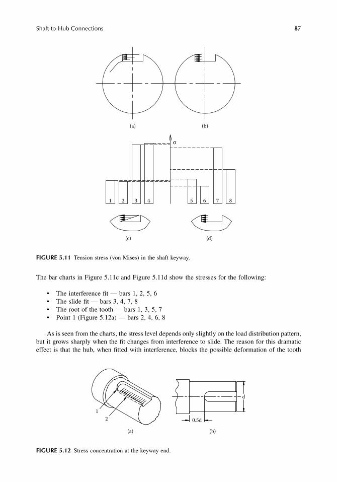
Shaft-to-Hub Connections 87
The bar charts in Figure 5.11c and Figure 5.11d show the stresses for the following:
• The interference fit — bars 1, 2, 5, 6• The slide fit — bars 3, 4, 7, 8• The root of the tooth — bars 1, 3, 5, 7• Point 1 (Figure 5.12a) — bars 2, 4, 6, 8
As is seen from the charts, the stress level depends only slightly on the load distribution pattern,but it grows sharply when the fit changes from interference to slide. The reason for this dramaticeffect is that the hub, when fitted with interference, blocks the possible deformation of the tooth
FIGURE 5.11 Tension stress (von Mises) in the shaft keyway.
FIGURE 5.12 Stress concentration at the keyway end.
(a) (b)
1 2 3 4 5 6 7 8
(c) (d)
σ
(a) (b)
d
1
2 0.5d
9563_C005.fm Page 87 Monday, August 6, 2007 4:21 PM

88 Machine Elements: Life and Design
in a radial direction (deformed contour is shown in Figure 5.13a, curve 1). When the hub is slidefitted, the deformation of the tooth is not restricted by the hub (see curve 2 in Figure 5.13b), andthe deformation at the same load is much bigger.
When the tooth deforms, it pulls the end fillet of the keyway. In Figure 5.12a, the deformedcontour of the keyway is represented by dashed line 2. The aforementioned point 1, where thetension stress is maximal, belongs to the keyway contour and the shaft neck surface, so the materialat this point suffers from both high stress and surface damage caused by IFC (fretting and others;see Chapter 2). These damages are related to the microslip in the connection and concentrated atthe end area of the connection where the transmitted torque is maximal. If the end of the keywayis moved away from the end of the connection (Figure 5.12b), the fatigue strength of the shaft maybe increased by 50–70%.6
5.3.4 STRENGTH OF HUB NEAR THE KEYWAY
Undoubtedly, strength problems are usually concerned with the shaft, but sometimes hub failuresalso are observed. Figure 5.14 shows the von Mises and maximal principal stresses in the keywayfillet calculated using FEM.
FIGURE 5.13 Keyway deformation under load.
FIGURE 5.14 Stress in the keyed hub.
(a)
1 2
(b)
2001.35
D/d
1.4 1.5 1.6
300
400
500
600
σ MP
a
1.35 1.51.4
D/d
1.6
300
200
400
500
1.35 1.51.4
D/d
1.6
300
200
400
500
1.35 1.51.4
D/d
1.6
300
200
400
500
f = 0.05
von-Mises stress
f = 0.1 f = 0.2 f = 0.3
1.5
300
1.35200
σ MP
a
400
500
600
300
1.61.4
D/d
1.5200
1.35 1.4
f = 0.05
500
400
500
400
200
300300
1.4
D/d
1.6200
1.35
D/d
1.5 1.6
Maximal principal stress
f = 0.1
400
500
f = 0.2
D/d
1.35 1.4 1.5 1.6
f = 0.3
700
600 600 600
1
3
1
2
3
1
23
1
2
3
1
2
3
1
3
1
2
3
1
3
2
22
9563_C005.fm Page 88 Monday, August 6, 2007 4:21 PM

Shaft-to-Hub Connections 89
The parameters of the key joints are as follows: shaft diameter d = 100 mm, hub diameter Dis variable (see Table 5.1), key dimensions 28 × 16 mm, fillet radius r = 1.5 mm. The length ofthe connection L = 120 mm. The connection is press-fitted, and the interference is changingdepending on the hub diameter, so as to achieve nearly the same surface pressure in all cases.
The stresses are calculated for different values of the friction coefficient (f = 0.05, 0.1, 0.2, and0.3) and for three loading conditions: torque transmitted T = 0 (the hub is stressed by the press fitonly, curves 1), 3750 N⋅m (curves 2), and 7500 N⋅m (curves 3).
From these charts one can see not only that the outer diameter of the hub influences significantlythe stress level (this was clear a priori), but also that the friction coefficient is a very strong factor,because it characterizes (together with the surface pressure) the ability of the friction forces totransmit the entire torque or most of it. Figure 5.15 shows the stresses at T = 7500 N⋅m. It is seenthat at f < 0.1, where the load capacity of friction forces becomes less than the torque applied, thestress in the keyway fillet grows quickly. This demonstrates once again, as stated already, thenecessity of press fit in KJs able to transmit the entire torque by friction forces; some safety marginis welcome.
Let’s compare the fatigue strength of the hub with that of the shaft.
EXAMPLE 5.4
We take for this analysis one of the cases calculated previously: d = 100 mm, D/d = 1.6, f = 0.2(after some on-period), and T = 7500 N⋅m. The material of the hub: SAE 4130, normalized, tensilestrength Su = 622 MPa, and yield point Sy = 484 MPa. The von Mises stress in the hub equals σ1
= 250 MPa when unloaded and σ2 = 350 MPa when transmitting the torque. If the torque (becauseof torsional vibrations) varies cyclically by, say, 15%, the stress amplitude equals
The maximal stress equals σmax = 350 + 15 = 365 MPa < Sy. Thus, the requirement for staticstrength of the hub is fulfilled.
TABLE 5.1Parameters of Calculated KJs
Hub diameter D, mm 135 140 150 160Interference (diametral), mm 0.094 0.088 0.076 0.070Surface pressure (by Lame), MPa 41.6 42.3 41.4 41.8
FIGURE 5.15 Stress in the keyed hub (T = 7400 N ⋅ m).
σ σ σa = − =( ) .2 1 0 15 15 MPa
2000.05
f
0.1 0.2 0.3
300
400
500
600
σ MP
a
von-Mises stress
300
σ MP
a
400
500
600
700
D = 135 mm140150160
0.05 0.20.1
f
0.3
D = 135 mm
160150140
Maximal principal stress
9563_C005.fm Page 89 Monday, August 6, 2007 4:21 PM

90 Machine Elements: Life and Design
What about the fatigue? We can determine the fatigue limit of this steel approximately asfollows (see Chapter 12, Subsection 12.1.2):
The fatigue limit of the part equals (see Chapter 12, Subsection 12.2.4):
whereKS = surface quality factor = 0.8 (see Chapter 12, Subsection 12.2.1)Kd = dimension factor = 0.9 (see Equation 12.58 in Chapter 12, Subsection 12.2.2)Ke = effective stress concentration factor (Ke = 1 in this case because the stress is the real maximal
stress determined using FEM)
If we neglect the mean stress (for the sake of simplicity and because its influence is weak; seeChapter 12), the safety factor of the hub against fatigue failure equals
So the hub strength doesn’t worry us. What about the shaft strength? If the shaft is loaded withthe torque only, the shear stress equals
(Note: T = 7500 N⋅m = 7500 ⋅ 103 N⋅mm. We had to convert the torque units into N⋅ mm, becausethe diameter d is expressed in mm.) Taking the stress amplitude as 15% of the mean stress, weobtain the shear stress amplitude: τa = 0.15 ⋅ 38.2 = 5.73 MPa.
Let’s assume that the shaft is made of SAE 4340 heat-treated to HRC 28–35. For this steelSu = 880 MPa and Sy = 725 MPa. The fatigue limit equals
For the shaft, KS = 0.9 (ground surfaces), Kd = 0.9, and Ke = 3.5 (stress concentration factorfor the press-fit connection). Thus, the fatigue limit for the shaft equals
S Su− = + = ⋅ + =1 0 454 8 4 0 454 622 8 4 291. . ( ) . .MPa MPa
S SK K
KpS d
e− −=1 1,
S MPap− = ⋅ =1 2910 8 0 9
1210,
. .
nS
Ha
= = =−1 21015
14σ
τπ π
= = ⋅ ⋅⋅
=16 16 7500 10100
38 23
3
3
Td
MPa.
S Su− = + = ⋅ + =1 0 383 94 0 383 880 94 431. ( ) .MPa MPa
S p− = ⋅ =1 4310 9 0 9
3 599 7,
. ..
. MPa
9563_C005.fm Page 90 Monday, August 6, 2007 4:21 PM

Shaft-to-Hub Connections 91
Because
where S−1,τ = fatigue limit in shear (see Chapter 12, Subsection 12.1.2), and
Taking the amplitude of alternating shear stress as 15% of the mean stress, we obtain
From here, the safety factor of the shaft against fatigue failure equals
Hence, though the shaft is largely overdesigned, its safety factor is still less than that of thehub. But in most cases, the shaft is loaded not only by a torque, but also by a bending momentsimultaneously. Let us assume that the hub and the shaft are parts of the gear output shaft shownin Figure 4.1 (Chapter 4). The force developed in the gear mesh loads the shaft (in addition to thetorque) with a bending moment M = 5.2⋅106 N⋅mm and produces in it the bending stresses σa thatchange cyclically at each turn of the shaft:
The equivalent stress (see Chapter 12, Subsection 12.1.2),
And then the safety factor of the shaft equals
The safety factor of the hub remains unchanged (nH = 14).From this example, we clearly see why we don’t usually have problems with the hub strength:
it is loaded nearly statically. But sometimes, for example, when the torque transmitted is reversibleand the press fit is not so tight as to transmit most of it by friction forces, the stress amplitude inthe hub increases immensely, and its strength may become insufficient.
In some cases, the keyway is placed in the nearest vicinity of the application of a cyclic loadas shown in Figure 5.16a. In this case, the round pins shown in Figure 5.16b can be preferable.
SS
−
−
=12
12
3,τ
S− = =1
99 7
357 6,
..τ MPa
τa = ⋅ =38 2 0 15 5 73. . . MPa
nS
Sa
= = =−1 57 65 73
10, ..
τ
τ
σπ πa
Md
= = ⋅ ⋅⋅
=32 32 5 2 10100
533
6
3
.MPa
σ σ τe a a= + = + ⋅ =2 2 2 23 53 3 5 73 54. MPa
nS
Sp
a
= = =−1 99 754
1 85, ..
σ
9563_C005.fm Page 91 Monday, August 6, 2007 4:21 PM

92 Machine Elements: Life and Design
5.3.5 ROUND KEYS (FIGURE 5.17)
Round keys are used for permanent joints, because the holes are drilled and reamed in the shaftand hub together. The connection with round keys is less detrimental to the strength of the shaftand hub and may be used for thin-walled parts, provided that the needed load capacity of the IFCmay be practically achieved.
The diameter of keys dk is recommended within (0.08–0.15)d, and the length lk = (3–5)dk. Themaximal bearing stress equals
(5.11)
where n is the number of keys.You can ask, where is this formula from? Why 16 and not 17 or, say, 24? Oh, the derivation of
the formula (Equation 5.11) is really simple. First, look at Figure 5.17b. Hub 1 rotates relative to
FIGURE 5.16 Key joints of thin-walled parts.
FIGURE 5.17 Round pins.
(a) (b)
σπmax = 16T
d d l nk k
(a) (b)
(c)
1a
a
2
s = smaxsina
smax
9563_C005.fm Page 92 Monday, August 6, 2007 4:21 PM

Shaft-to-Hub Connections 93
shaft 2 under load (owing to elastic deformations) by a very small angle. This angle is so small thatthe movement in the vicinity of one key can be considered as translational displacement in a tangentialdirection (assuming also that the key diameter is small as compared to the diameter of the connection).This displacement measured in tangential direction is nearly the same at all points, but the bearingdeformation in contact of the hub and the key, which is measured perpendicular to the key surface(in Figure 5.17b, this area is blackened), is obviously proportional to sin α. Because the stress isproportional to the deformation, we can write the formula for the bearing stress (see Figure 5.17c):
Thus, at α = 0, σ = 0; at α = π/2, σ = σmax.Force is the product of pressure by area. The infinitesimal area on the key surface is
From here, the infinitesimal force (applied to the infinitesimal area perpendicular to the surface ofthe pin)
The tangential component of this force, dFt, which opposes the tangential force created by thetorque, equals
The tangential force taken by one pin equals
The obvious equilibrium condition is
From here, Equation 5.11 is obtained directly. In reality, the pressure distribution is not exactlysinusoidal because the radial components of the key pressure deforms the hub in the radial direction,and the pressure concentrates more in the vicinity of the joint diameter. Well, it is too complicatedto get into any deeper.
5.4 SPLINED JOINTS
Splined connections are made in two types: straight (Figure 5.18a) and involute (Figure 5.18b).The straight spline has less friction force when moving the hub axially under load. The involutespline is stronger (because of the larger number of teeth) and less detrimental to the strength of
σ σ α= max sin
dA r d ld
l dkk
k= ⋅ ⋅ = ⋅α α2
dF dAd l
dk k= ⋅ =σ σ α αmax sin2
dF dFd l
dtk k= ⋅ =sin sinmaxα σ α α2
2
FTn0
2=
F dFd l
d dtk k
k0
0
2
2
0
2
2 8= = ⋅ =∫ ∫
π π
σ α α π σ/
max
/
maxsin llTnk = 2
9563_C005.fm Page 93 Monday, August 6, 2007 4:21 PM

94 Machine Elements: Life and Design
the shaft. The effective stress concentration factor for the involute spline is about 1.7 times lessthan that for the straight spline.4
Performance capabilities of SJs depend strongly on the kind of load transferred — whether itis a torque only or torque with a radial force. The two kinds of loading are considered separatelyin the following subsections.
5.4.1 SJS LOADED WITH TORQUE ONLY
Figure 5.19 shows several examples of tightened SJs that are loaded (at first sight) with a torqueand a radial force. But notice the following: in all these connections, the centering of the hubrelative to the shaft is made using additional surfaces, so the spline doesn’t participate in thetransmission of the radial force.
In Figure 5.19a, flange 1 is centered on the left directly on shaft 2 and, on the right, throughinsert 3 pressed into flange 1. The insert is used to ease manufacturing by allowing the inner splineto be broached. Tightened nut 4 is locked with special washer 5, which is provided with inner andouter protuberances engaged with corresponding slots in the shaft and nut. Snap ring 6 holds thewasher in place.
FIGURE 5.18 Spline shapes.
FIGURE 5.19 Centering of spline connections using additional surfaces.
(a) (b)
dm dm
hh
(c)
(a)
2 1 3 4
5
6
15
7 8 9
11
10
12
1413
16
(b)
9563_C005.fm Page 94 Monday, August 6, 2007 4:21 PM

Shaft-to-Hub Connections 95
Figure 5.19b represents a shaft of a triple-speed drive. In this design, pinion 7 is centered onthe left directly on the shaft and, on the right, through the hub of pinion 8. The latter is centeredon the right through insert 9. All these parts are tightened with nut 10 that is locked with a deformablewasher 11.
In the design shown in Figure 5.19c, gear 12 is centered relative to shaft 13 using split cones14 and 15. To make dismantling easier, the angle of the cones is made larger than the coefficientof friction. Usually, the vertex angle is 30° and 60° for cones 14 and 15, respectively. The conesmay be made of bronze or brass to discourage fretting. To reduce to a minimum the possiblemicroslip in the connection under load, nut 16 should be tightened strongly.
Figure 5.20 shows the intermediate shaft of a tractor gear box. Gears 1, 2, and 3 are mountedon shaft 4 through rolling bearings, so that they can rotate independently of the shaft. When oneof these gears is brought into operation, it is made to rotate with the shaft by coupling 5 or 6 soas to transmit torque. These couplings are connected to shaft 4 through splined sleeves 7 and 8,and they can be engaged or disengaged by shifting their axial positions.
In all, there are seven SJs loaded only with torque:
• Shaft 4 with sleeves 7 and 8• Coupling 5 with sleeve 7 and gear 1 (when engaged)• Coupling 6 with sleeve 8 and gears 2 and 3 (when engaged)
The connections of sleeves 7 and 8 are centered relative to the shaft by the outer diameter of thesplines, tightly fitted and tightened with nut 9. But in the rest of the connections listed, there mustbe sufficient clearances to enable free axial movement.
SJs usually fail because of tooth wear; therefore, the strength of SJs is checked by calculatingthe bearing stress. The tangential force is
whereT = torque transmitted (N ⋅ mm)dm = mean diameter of the SJ (mm)
The working area of the teeth that take this force is
FIGURE 5.20 Intermediate shaft of tractor gear box.
FT
dtm
= 2
A hln=
1 2 3 45 6
7 8
9 10 11
9563_C005.fm Page 95 Monday, August 6, 2007 4:21 PM

96 Machine Elements: Life and Design
whereh = height of the active surface of the tooth minus the chamfers (measured in radial direction)l = engaged length of the teethn = number of teeth
From here, the nominal bearing stress equals
(5.12)
The authors can’t refrain from reminding the reader of the necessity to keep compatibledimensions for all the homogenous terms of an equation. In particular, in Equation 5.12, if youchoose newtons and millimeters, all the dimensions (dm, h, and l) must be expressed in millimeters(mm), and torque, T, in newton millimeters (N ⋅ mm). The result will be obtained in newton permillimeter, squared (N/mm2 = MPa). If the torque is given in newton meters (Nm) and you don’twant to change this, all the dimensions listed previously must be given in meters, and the resultwill be expressed in newton per meter, squared (N/m2 = Pa). If you choose pounds and feet —well, you know what to do!
Involute splines usually have a 30° pressure angle and 1.2m tooth height (m is the module ofthe teeth, given in millimeters; conformably to the AGMA system, m = 25.4/P where P is thediametral pitch). The engaged height of the teeth h = m, and the mean diameter dm = m ⋅ n, so thenumber of teeth n = dm/m. Substitution of these data into Equation 5.12 gives the expression forthe nominal bearing stress:
(5.13)
Sometimes, gear teeth are used to form a spline joint. The pressure angle of these teeth is 20°,and the tooth height, 2.25m. The engaged height h = 2m, i.e., twice as much as in spline teeth.Therefore, this joint is more wear resistant (because the bearing stress is half as large as in theusual SJs), but these teeth are more “breakable” and more sensitive to misalignment. Therefore,when there is considerable angular misalignment in the connection, this option (with 20° teeth) isused with crowned (barrel-shaped) teeth (see Figure 5.8). Teeth with engaged height h = 1.6m arealso in use.
Equation 5.12 and Equation 5.13 are derived with the assumption that the contact pressure isdistributed uniformly over the working surfaces of the teeth. To find the maximal bearing stress,some correction factors are used:
(5.14)
Factor kT is used to consider the unevenness of load distribution between the teeth caused byerrors of shape and the angular position of the teeth. For nonwearing SJs at the usual accuracy,kT = 1.3–1.4. If there is some wear of the spline, the more loaded teeth become more worn, andafter a run-in period, all the teeth will be loaded uniformly. So for this case, kT = 1.
Load distribution may also improve in nonwearing joints because of local plastic deformationof the overloaded surfaces. Therefore, in all cases, it is worth marking the parts so as to assemblethe spline always in the same position.
Factor kL is intended to consider the unevenness of load distribution along the teeth caused bydifferent twisting of the shaft and the hub. (This phenomenon is similar to that in IFC; seeChapter 2.) The larger the length of the SJ, the greater is the kL value.
σnomm
FA
Td hln
= = 2
σnomm
Td l
= 22
σ σmax = nom T Lk k
9563_C005.fm Page 96 Monday, August 6, 2007 4:21 PM

Shaft-to-Hub Connections 97
The kL value depends on the rigidity of the parts and the teeth. For example, if the number ofteeth is 6, their compliance is greater, and kL is less than if the number of teeth is, say, 16. Forinvolute splines that have a relatively large number of teeth, the factor kL may be determinedapproximately from this equation:
(5.15)
For example, l/d = 1, kL = 3. More exact calculation can be done using FEM.In wearing joints that transfer a constant torque, the teeth will run in, and for them, kL = 1. If
the torque value changes considerably, the load distribution along the teeth will never becomeuniform. Half of the kL value obtained from Equation 5.15 may be taken in this case just byguesswork.
5.4.2 SJS LOADED WITH TORQUE AND RADIAL FORCE
Examples of this type of SJ are given in Figure 5.20; gears 10 and 11 are connected with shaft 4by splines that transmit both the torque and the force applied to the teeth.
Let’s imagine that a spline is manufactured and assembled with absolute accuracy. If thisspline transmits only torque, the load is distributed uniformly between the teeth (Figure 5.21a). Inthis case, the shaft and the hub are coaxial and the vector sum of all forces applied to the teethequals zero. If the SJ is also loaded with a radial force, the load distribution between the teeth mustbe nonuniform, because the vector sum of the tooth forces must equal the loading radial force.(Nobody has cancelled Newton’s 3rd Law!) Figure 5.21b shows how the picture changes when theradial force is applied. The hub shifts relative to the shaft in the direction of the force by somesmall amount ε. At this force, the load of teeth 2 and 3 increases (in the figure, it looks as aninterference of the teeth surfaces that were before in touch, but, in reality, it symbolizes increasedcontact deformation). The load of teeth 5 and 6 decreases because their working surfaces move
FIGURE 5.21 Load distribution in spline joints.
kldL ≈ 3
1
6
5
4
3
2
T T T T
Fr
(a) (b)
Rh
Rs
1
6
5
4
3
2
(c)
qT
qF
α
r = 0.5 dm
α
ε
9563_C005.fm Page 97 Monday, August 6, 2007 4:21 PM

98 Machine Elements: Life and Design
apart (in the figure, a gap appears between the surfaces; in reality, it is not necessarily a gap, butit may be just a decrease in contact deformation; but a gap may arise as well, if the radial force islarge enough). The load of teeth 1 and 4 should not change because the distance between theworking surfaces doesn’t change as a result of radial displacement of the hub.
As the joint rotates relative to the vector of the radial force, the center of the hub describes acircle of radius ε relative to the shaft, and the working surfaces slip cyclically. Each turn of thejoint conforms to one cycle of slippage, and each cycle is accompanied by a certain wear of theworking surfaces.
The aforesaid is wholly correct when the hub is centered relative to the shaft by the working(side) surfaces of the teeth. But if the hub is centered by any additional surfaces (for example, bythe outer diameter of the teeth, when Rs = Rh [see Figure 5.21b], which excludes any radialdisplacement of the hub), the spline transmits only the torque, and the radial force is taken by thecentering surfaces. In practice, there is often a mixed design: the hub is centered by the outer (orsometimes by the inner) diameter of the teeth, but there is a small clearance (Rh is a bit biggerthan Rs) to ensure easy assembly and, if needed, easy axial movement of shifted gears. If there isa radial force, the hub can move in a radial direction within the clearance, and the greater theclearance, the larger the radial displacement, leading to slippage and wear. Therefore, it is desirableto decrease the clearance between the centering surfaces. It should be noticed that the cyclic motionof the hub relative to the shaft brings about wear to the centering surfaces as well. This means thatthe initially small clearance between the centering surfaces will increase with time and the wearprocess will accelerate exponentially.
But what can one do! Everything has its working life. And if we sometimes feel sorry in this“connection,” the SJ is not the object we usually grieve for.
It is seen from Figure 5.21b that the “change in distance” between the working surfaces ofthe mating teeth associated with the hub radial displacement is proportional to sin α. (For teeth1 and 4, sin α = 0, so their load doesn’t change.) To derive the equations for the maximal andminimal tooth force, let’s assume that there are infinitely many teeth. Then we consider the loaddistribution from torque T and from radial force Fr separately. The unit tangential force from thetorque (per millimeter of the SJ’s circumference) assuming its uniform distribution (seeFigure 5.21c) is
The unit tangential force from the radial load is
The vector sum of the qT forces is zero; so the equilibrium condition lies in the fact that thescalar sum of the qF forces must be equal to Fr. The resolution of forces qF by vertical and horizontalcomponents shows that the horizontal components on the right and on the left get balanced. Thesum of the vertical components qFvert shall counterbalance the force Fr:
The infinitesimal force equals
qT r
rTr
N mmT = =//
2 2 2π π
q q N mmF F= max sin /α
q q qFvert F F= =sin sinmaxα α2
df q ds q rd q r dFvert Fvert F= = = ⋅α α αmax sin2
9563_C005.fm Page 98 Monday, August 6, 2007 4:21 PM

Shaft-to-Hub Connections 99
From the equilibrium condition,
So the maximal and the minimal unit tangential loads are
(5.16)
Let’s denote kR as the factor that considers the unevenness of load distribution between theteeth that is caused by radial force. Because r = 0.5dm,
(5.17)
If we would like to know the maximal tangential force applied to one tooth, we can calculateit from Equation 5.16, taking into consideration that the force is equal to the product of the unitload and the length of an arc. The length of arc per tooth
Thus, the max tooth force equals
An additional unevenness of load distribution along the teeth is caused if the radial force vectoris displaced from the middle of SJ by some amount e, (Figure 5.22a). Such a design should be avoidedbecause uneven wear of the spline will result in misalignment of the hub relative to the shaft. If thehub belongs to a gear, the misalignment of the gear teeth may cause its premature failure. It may bepreferable to make the spline shorter but symmetrical relative to the radial force (Figure 5.22b).
For a spur gear that is mounted on a splined shaft (such as gears 10 and 11 in Figure 5.20),radial force Fr is a force Fg applied to the gear teeth. This force equals
F df q r d rq
qF
r F F
F
= = ⋅ =
=
∫ ∫0
2
0
2
2
π π
α α πmax max
max
sin
rr
rN mm
π/
q q qTr
Fr
q q qTr
T Fr
T F
max max
min max
;= + = +
= − =
2
2
2π π
π 22− F
rr
π;
kq
q
Tr
Fr
Tr
F rT
F d
TRT
r
r r m= =+
= + = +max 2
2
12
12
2
π π
π
sd
nm= π
F q sTr
Fr
d
n nTd
Fr m
mrmax max= = +
= +2
22π π
π
FT
d
T
dgg g
=°
≈220
2cos
9563_C005.fm Page 99 Monday, August 6, 2007 4:21 PM

100 Machine Elements: Life and Design
(Here dg is the pitch diameter of the gear.) From the previous equation, also taking into considerationEquation 5.17,
(5.18)
From Equation 5.18, we can see that the bigger the ratio dm/dg, the greater is the unevennessof load distribution between the teeth of the SJ.
5.4.3 ALLOWABLE BEARING STRESSES IN SJS
Prestressed SJs that practically don’t wear are calculated for maximal bearing stress. Because inthese joints, the centering is usually performed using additional surfaces (see Figure 5.19), thespline transmits the torque only, and the bearing stress may be determined using Equation 5.12 toEquation 5.14. This stress should not exceed the yield point of the material divided by some safetyfactor of about 1.2–1.4. It is clear that for this calculation, the maximal torque, including the possiblevibrations and momentary overloads, must be taken into account.
If the hub may move relative to the shaft, the spline is calculated both for the maximal bearingstress and for wear. The first one is performed just as for the prestressed joints, but if the SJ isloaded by a radial force as well, the factor kR should be taken into account.
For the wear calculation, the momentary loads should not be considered. Usually, the calculationis based on the maximal of the long-acting loads typical of the work cycle. The contact stress inthis case may be determined using Equation 5.12 to Equation 5.14, where kL = kT = 1. But if thereis a radial force applied to SJ, the factor kR must also be included.
FIGURE 5.22 Influence of toothed rim dissymmetry on a spline connection.
(a)
e
(b)
kd
dRm
g
= +1 2
9563_C005.fm Page 100 Monday, August 6, 2007 4:21 PM

Shaft-to-Hub Connections 101
The allowable bearing stress for wearing joints depends on the wear resistance of the teeth andthe needed service life. The determining factor for the wear resistance is the hardness of the workingsurfaces of the teeth (i.e., their flanks). These surfaces are often treated to produce a hard layer (asin induction hardening, carburizing, or nitriding) and/or coated with materials that decrease frictionand wear. Besides, the wear rate depends on the amplitude of the cyclic displacement of the hubrelative to the shaft. It may depend on the dm/dg ratio (for gears), or it may be determined byfunctional needs (e.g., SJs of vehicle cardan shafts or SJs used to connect shafts with a certainmisalignment; see Figure 5.23 and Chapter 6, Figure 6.43). Wear resistance is also greatly dependenton lubricant quality and cleanness.
Usually, calculation of the allowable bearing stress is based on experimental and service data.As a guide, for tempered steels (HRC 30–35), the allowed bearing stress may be within the limitsof 15 to 30 MPa, and for case hardened teeth (HRC 56–61), 40 to 60 MPa. It doesn’t mean thatthe stress can’t be 100–150 MPa, or even higher at certain conditions, but everything should bechecked experimentally.
5.4.4 LUBRICATION OF SJS
The mechanism of lubrication of metals is described in Chapter 6, Subsection 6.3.2, in which theabsolute necessity of lubrication, at least before assembly, becomes completely clear. For heavilyloaded prestressed joints, where micromovements are expected, a permanent access to liquidlubricant may be needed (Figure 5.19b).
If the hub is expected to move relative to the shaft, the spline may be greased or lubricatedwith liquid oil. In joints placed outside a mechanism (for example, in cardan shafts), the splinesare generally greased for life or with a greaser that enables periodical relubrication.
Grease lubrication simplifies the design of the joint: there is no need for an oil tank, or oilsupply devices; the seals are much simpler and, even if the seal is worn a bit, no leakage can beobserved. But the heat removal in this case is relatively small. Therefore, if heat release in the joint
FIGURE 5.23 Lubrication of loose spline joints.
3 1 2 6
8
5
7
9
10
4
9
10
9563_C005.fm Page 101 Monday, August 6, 2007 4:21 PM

102 Machine Elements: Life and Design
is high (because of high speed, increased cyclic movement in the joint, or both), the liquid lubricationsystem should be used to take the heat off effectively.
When placed inside an oil-lubricated mechanism, the SJ is lubricated with oil as well. Figure 5.23shows a typical connection of two gears, 1 and 2, by torsion bar 3 with involute splines 4 and 5on its ends. Gears 1 and 2 are not concentric because the radial forces applied to the gears aredirected oppositely, and the radial displacement of the gears in their sliding bearings is opposite.As a result, there is a misalignment and cyclic movement with the frequency of rotation in the SJs.The lubricating oil comes from oil duct 6 to the sliding bearing of the gear and at the same timeto oil sprayer 7 (through the ducts in the housing and cover 8). The sprayer has two nozzles: one,central, jets oil to spline 4; the other, a side nozzle, supplies oil to spline 5. Under centrifugalforces, the oil fills up the annular spaces formed inside the torsion bar and then through radialholes 9 flows to circular grooves 10. These grooves are turned both in the inner and outer splines.The oil fills up the grooves and flows out from there through the backlashes in the splines, takingoff the heat and washing out all the wear debris.
REFERENCES
1. Grechistchev, E.S. and Iliashenko, A.A., Interference Fit Connections, Machinostroenie, Moscow,1981 (in Russian).
2. Birger, I.A. and Iosilevich, G.B., Threaded Joints, Machinostroenie, Moscow, 1973 (in Russian).3. Bossard, Metric Fasteners for Advanced Assembly Engineering, Bossard Ltd. Fasteners, 1990.4. Birger, I.A., Shorr, B.F., and Iosilevich, G.B., Calculation of Machine Elements for Strength,
Mashinostroenie, Moscow, 1979 (in Russian).5. Timoshenko, S. and Woinowsky-Krieger, S., Theory of Plates and Shells, McGraw-Hill, New York,
Toronto, London, 1959.6. Kogaev, V.P., Calculations for Strength at Stresses Variable with Time, Mashinostroenie, Moscow,
1977 (in Russian).
9563_C005.fm Page 102 Monday, August 6, 2007 4:21 PM

103
6
Supports and Bearings
At the beginning of this chapter, two technical terms should be defined:
bearing
and
support
. Here,a bearing is considered a part or a unit that serves directly as an interface between the rotating andstationary parts (say, between the shaft and the housing). A support is considered a unit that includesat least one bearing (maybe two or more), adjoining part of a housing, and possibly other partsneeded for the axial fixation of the bearings, end play adjustment, etc. No other terms need anyelucidation.
6.1 TYPES AND LOCATION OF SUPPORTS
Usually, shafts have two supports. Each support fixes the adjoined part of the shaft in a radialdirection. Additionally, the support may fix this part in one axial direction (type F1), in both directions(type F2), or not to fix in the axial direction at all (type NF).
For shafts fixed in the axial direction, a combination of supports, F2
+
NF (Figure 6.1a) or twoF1 supports (Figure 6.1b), is used. In the latter case, the axial play that is set when assemblingmust be greater than the probable difference in thermal deformations of the shaft and the housing;otherwise, the supports may become jammed and damaged. This difference in thermal expansionscan’t be exactly determined because it depends on the power loss in the mechanism, environmenttemperature, cooling conditions, and so on. As a rule, if the shaft needs an exact axial fixation,such a design is not acceptable.
A shaft may have two NF supports if it is joined to another part, which is fixed axially, forexample, by a flange connection to another shaft (Figure 6.1c) or by the engagement of two double-helical gears (Figure 6.1d). Error of axial location of such a shaft includes axial play of the axiallyfixed part plus the possible clearance in the connection of the two parts. Specifically, in the flangeconnection, the clearance is zero. But in the engagement of double-helical gears (Figure 6.1d), thesituation is more complicated. The nominal position of teeth 1 (belonging to the pinion) relativeto teeth 2 of the gear wheel is symmetric (Figure 6.1e). In this position, which is realized underload, both the right and the left teeth of the pinion are in contact with the corresponding teeth ofthe gear. If the gear is unloaded, pinion 1 may be moved relative to gear 2 in an axial direction byamount
X
(Figure 6.1f). In this position, pinion teeth 1 and gear teeth 2 are in contact from aboveon the left and below on the right side. Obviously, the pinion may be moved by the same distancein the opposite direction. The total axial movement of the pinion is given by
where
Z
=
backlash magnitude in the engagement (mm)
ψ
=
helix angle
ϕ
=
pressure angle
For example, if the backlash magnitude
Z
=
0.5 mm,
=
30
°
, and
ϕ
=
23
°
, the possible axialmovement of the pinion with respect to the gear equals 1.09 mm. Under load, axial forces
F
a
movethe pinion to a symmetric position depicted in Figure 6.1e. In this position, the teeth on the left
2XZ=
sin cosψ ϕ
ψ
9563_C006.fm Page 103 Wednesday, July 25, 2007 4:17 PM

104
Machine Elements: Life and Design
and on the right are transmitting the same load, and forces
F
a
are even on both sides. Gear tolerances(such as radial and lateral runouts, variations in tooth thickness and helix angle, and others) makethe pinion oscillate with small amplitude during rotation to keep the symmetric position. Thismovement should not be hindered, because it is aimed at achieving equality of forces
F
a
and,consequently, of even load distribution between the left and right teeth.
To put it more precisely, the complete equality of forces
F
a
is not achieved because of frictionalforces in the teeth, bearings, and couplings. This point is discussed more comprehensively inSubsection 6.2.3 (friction in roller bearings; see also Example 6.3) and Chapter 7, Section 7.8.
A supported section of a shaft may move relative to the housing within limits determined byclearances in the support, runout of the bearings, and elastic deformations of bearings and otherparts of the supports. Therefore, selection of a distance between supports and their location relativeto shaft-mounted elements (gears, cams, pulleys, and so on) may have a dramatic effect on theshaft loads and on the shaft’s actual position (alignment) relative to the housing. Let’s explore thisin more detail.
The alignment of a shaft in radial supports, which have clearances and certain compliances,depends on the magnitude and direction of the radial forces applied to the supports. In the simplestcase, when the shaft rotates in radial bearings and the reactions at the supports,
R
1
and
R
2
, havethe same direction (Figure 6.2a), the angle of misalignment of the shaft relative to the housing,
Θ
,is determined by the difference in radial clearances and elastic deformations of the supports:
where
∆
1
and
∆
2
are the radial displacements of the bearing necks of the shaft in supports 1 and2, respectively, under the action of forces
R
1
and
R
2
, and
L
=
spacing of the bearings.If the supports are made with plain bearings, the inequality of vectors
R
1
and
R
2
may cause anadditional misalignment of the shaft because of the different eccentricity of the shaft journals inthe bearings and the different angular position of the point of minimal clearance.
FIGURE 6.1
Examples of axial fixation of shafts.
(a) (b)
(d)
(c)
F1 F1
NF NF
F1 F1
1
2
(e) (f )
NF NFF2
NF
Flange connection
F2 NFShaft
1
2
12
Fa
Z
X
ψ
Θ ∆ ∆= −1 2
Lrad( )
9563_C006.fm Page 104 Wednesday, July 25, 2007 4:17 PM

Supports and Bearings
105
If the shaft is loaded as shown in Figure 6.2b to Figure 6.2d, the reactions at the supports mayhave an opposite direction, and in these cases, the angle of misalignment will be much bigger:
To decrease the misalignment, the clearances in the supports should be made as small aspossible, and the stiffness of the supports and spacing
L
should be increased as much as practical.Not always is the increased spacing of supports welcomed. If the shaft is exposed to bending
moments, its increased length may impair the alignment of machine elements mounted on it. Forexample, the misalignment angles
Θ
b
in the middle of the bevel pinion, which is caused by bendingof the shaft by forces
F
r
and
F
a
, is given by
(The dimensions are shown in Figure 6.2d; angles
Θ
b
are not signed.)The final misalignment of the pinion results from the vector summation of these bending-
conditioned angles with the supports-conditioned angle
Θ
, and the optimal ratio of dimensionsshould be found in each case, separately.
E
XAMPLE
6.1
Figure 6.3a shows a double-geared planet wheel with straight teeth. As applied to the topic underdiscussion, this planet wheel represents a shaft, which has two supports of type F1 placed inside
FIGURE 6.2
Shaft misalignment due to displacement in bearings.
(a) (b)
(c) (d)
(e)
Fr
Fa
R1
R2F1
F2
Fr
Fa
da
CL
R1
R2
Fr
Fa
Θ
L
Fr
R1 R2
Θ
L
Θ ∆ ∆= +1 2
L
Θ Θb Frr
b Faa aF C
EIL C
F d
EIL C, ,( ); ( )= − + = +
62 3
63
9563_C006.fm Page 105 Wednesday, July 25, 2007 4:17 PM

106
Machine Elements: Life and Design
it and two toothings from the outside. This planet wheel doesn’t need an exact axial fixation. Thedirection of forces applied to the teeth is shown in Figure 6.3b (to make the scheme clearer, onlythe tangential components are depicted). Force
F
3
is relatively small, and the planet wheel is mainlyloaded by forces
F
1
and
F
2
. The designer of this gear had placed the bearings so that each of themis symmetric about one of the toothings (Figure 6.3a). During the test, a strange phenomenon wasfound: after short-term work under heavy load, the planetary gear appeared seized up, so that itwas impossible to turn it by hand. (However, a good blow by heavy hammer would unlock it.)Dismantling revealed that the roller bearings of the planet wheels had severe smearing on theirraceways concentrated on a third of their width. In addition, some of the bearings had brokenshoulders of the inner rings. These damages were brought about by angular misalignment (skewing)of the planet wheel relative to its axle, which led to the skewing of outer rings of the bearings relativeto their inner rings. This trouble was eliminated by increasing the bearing spacing (Figure 6.3c), whennot only the angle of skew but also the load of the bearings was markedly decreased. The changewas made within the existing width of the planet carrier openings.
Now, as we have made certain how important it is to decrease the misalignment of a part, let’sconsider (just for a change) another example, in which, in contrast, the part should have the freedomto skew freely in any direction. Figure 6.3d shows a spur planet wheel supported by a singlespherical bearing installed symmetrically about the middle of the tooth. This design has a uniqueproperty: self-adjustment of the planet wheel relative to the mating gears (sun wheel and annulus)so that the load is evenly distributed along the teeth. This method may be used not only for planetwheels, but also for any idler. Uniform load distribution along the teeth, which is assured by thisdesign, enables the use of gears with an increased face width and correspondingly decreaseddiameters. This may be important when the radial dimensions of the drive are limited.
The question is why this design is not used for all spur planet wheels and idlers? There canbe several reasons for this. First, a spherical bearing of needed load capacity can’t always beinstalled inside the gear. Quite often, the idler should be installed on an axle with the bearingsplaced on both sides of the gear, where their diameters can be made much greater. Second, sphericalbearings are less suitable for high-speed applications than, for example, straight roller bearings.And third, perhaps, a certain inertia of the designer’s thinking and distrust of new, untried solutionsshould be mentioned. This approach is positive and helps prevent mistakes, but sometimes ithampers progress. Indeed, if some design is not used in such a trustworthy field as aviation or
FIGURE 6.3
Planet wheel bearings.
(b)
(c)
F1 F2
F3
(d)
Sun wheel
Planet wheel
Annulus
(a)
Annulus,
rotating
Annulus,
stationary
Double-geared
planet wheel
Sun wheel
9563_C006.fm Page 106 Wednesday, July 25, 2007 4:17 PM

Supports and Bearings
107
transportation engineering, the designer doesn’t feel confident enough to use it. At the same time,the design with idlers or planet spur gears supported by a single spherical roller bearing has beensuccessfully proved in low- and middle-speed drives.
Let’s come back to the usual design of shafts supported in two points. With respect to shaftmisalignment, one of the most unfavorable variants is an overhung loading (Figure 6.2d). Rollerbearings, when properly spaced (
L
≥
2
C
is recommended
1
), are able to position the shaft withreasonable accuracy; see Figure 6.15 (input shaft 6) and Figure 6.20a. Nevertheless, for bevel gears,one usually uses special tooth geometry with localized contact (for example, spiral bevel gears),which are less sensitive to misalignment. In addition, the gears should be adjusted during assemblyin such a way as to displace the contact pattern toward the vertex of the cone as shown in Figure 6.20a.Under load, the shaft becomes bent and displaced in the supports as shown in Figure 6.2d, andthen the real contact pattern is expected to move toward the base of the cone and to take up positionin the middle of the tooth length.
Shafts with an overhung load supported by sliding bearings may keep an aligned position underload if the sleeve bearings are not concentric (Figure 6.2e). The magnitude and direction of theeccentricity should be calculated so as to provide the needed location of the shaft. Such a designrequires nice calculation of the plain bearings, and the partial load conditions should be taken intoaccount as well. An additional point to emphasize is that the bearings must not have any wearwhile in service; otherwise, all this elaborate work becomes meaningless.
Overhung loads are usually avoided in heavily loaded mechanisms. In Figure 6.16c andFigure 7.31 (see Chapter 7), the gear is so designed that the bevel pinion is placed between twobearings.
As noted in the preceding text, the supports may be made of rolling bearings (RBs) or slidingbearings (SBs). The SBs are not as good at a low speed when the machine is starting or reciprocating,because in these cases, there is mixed or boundary friction, which is accompanied by wear andincreased heat generation.
“Less good” doesn’t always mean “bad.” For example, the piston pin bearing in piston enginesis usually made of a bronze sleeve and works successfully, in spite of relatively low speed andreciprocating motion.
SBs are more sensitive to the quality of the lubricating oil and to the mode of lubrication. Inmany cases, they need a pressure lubrication system with filtration to maintain lubricant cleanliness.At the same time, RBs content themselves at low and moderate speeds with splash lubrication orwith grease applied during assembly. For these reasons, small and midsize mechanisms are usuallyprovided with RBs, which have very low friction starting from zero speed.
Of fundamental importance is that RBs can work with very small clearances or even withprestressing. That allows the shaft to be positioned more exactly. RBs are not as good at high speed;their load capacity decreases (and service life is shorter because of the large number of cycles). Inaddition, the running temperature is higher. The reliability of RBs at a high speed is more influencedby errors of manufacturing and assembly, such as runouts and waviness of races, imbalance or poorcentering of cages, runouts of the shaft necks and shoulders, fit tolerances, accuracy of axial playadjustment, and so on. If the speed is more than two thirds of the catalog limit, considerable attentionshould be given to the working conditions of RBs; such factors as vibrations, poorly purified oil,insufficient (and also excessive) lubrication, and nonoptimal oil viscosity may cause the failure ofa bearing. In these cases, it is worth asking the bearing manufacturer for recommendations.
As opposed to RBs, the load capacity of SBs increases when the speed rises. In SBs, thecontinuous oil film that separates the shaft journal from the bearing is achieved safely at a highspeed. Under such conditions, the SB can work over a long period of time practically without anywear. Therefore, in large high-speed machines, in which heavy load and high speed are combinedwith a long service life, the SB is quite often the only acceptable type of bearing.
One of the controlling considerations is cost. Large SBs are much cheaper than RBs both inproduction and in maintenance. Early detection of an SB’s damage can be easily accomplished by
9563_C006.fm Page 107 Wednesday, July 25, 2007 4:17 PM

108
Machine Elements: Life and Design
measuring its temperature or by sampling metal particles in the oil. This enables the machine tobe stopped before significant damage occurs. The repair is usually cheap and consists of replacingthe damaged bearing sleeve. In contrast to SBs, the failure of RBs often comes with little warningand is accompanied by damage to other parts. The small radial dimensions and weight of SBs andtheir ability to dampen impact loads give them wide application in combustion engines, includingcar motors.
6.2 ROLLING BEARINGS (RBs)
Catalogs of RBs are provided with brief information concerning design, technical data, and direc-tions for use. This information must be taken into consideration. In the following text are discussedsome important factors for the reliability and durability of RBs that will help designers orientthemselves in the information given by the manufacturers.
6.2.1 D
ESIGN
OF
RB
S
Deep groove ball bearings (Figure 6.4a) consist of two rings, inner and outer, and a set of ballsbetween them, separated by a cage. Raceways are shaped closely to the balls; a cross section ofthe raceway represents an arc of circle with radius larger by 3% than that of the ball. The numberof balls depends on the possibility to put them in place. Figure 6.5 shows the stages of assembly:placement of the balls inside the “crescent” (Figure 6.5a), shifting of the inner ring to the centralposition (Figure 6.5b), and equal distribution of the balls around the circumference (Figure 6.5c).After that, the cage should be installed in place to keep the distribution of the balls even. The cageis made of two halves, put in from both sides of the balls and riveted together within intervalsbetween the balls.
If for some reasons the cage is destroyed in service, the assembly process may be reversed:the balls may gather and fall out of the bearing. In this case, the shaft will dangle with big amplitudeand destroy everything on its way. This feature of such bearings should be taken into considerationwhen thinking over possible emergency conditions. From this point of view, bearings with greaterquantity of balls or rollers are preferable; when the cage fails, the quantity of rollers keeps theinner ring concentric to the outer ring, and the shaft may remain in place until the bearing failureis revealed.
FIGURE 6.4
Basic types of rolling bearings commonly used in machines.
(a) (b) (c) (d) (e) (f )
(g) (h) (i) (j) (k)
9563_C006.fm Page 108 Wednesday, July 25, 2007 4:17 PM

Supports and Bearings
109
Single-row angular contact ball bearings (Figure 6.4b) and four-point bearings (Figure 6.4c)have more balls because the assembly conditions are better. The number of balls here is limitedby the strength of the cage between the balls. The main responsibility of the cage, which may bemade solid for these bearings, is to prevent contact between the rolling elements, because the highsliding velocity in their contact may result not only in high power losses but also in burns andscoring of their surfaces.
Bearings with straight or tapered rollers (Figure 6.4d to Figure 6.4f) have cylindrical or taperedraceways, respectively. These surfaces are usually modified to reduce the sensitivity of thesebearings to the misalignment of the rings. The modification consists of small removal (about severalmicrons) of metal at the ends of the raceways or the rollers. Nevertheless, roller bearings are verysensitive to angular misalignment of the shaft, which should not exceed 0.001 rad.
The function of the cage in roller bearings is to separate the rollers and to prevent skewing ofthe rollers relative to the bearing axis. (The latter function is also performed by the shoulders ofthe rings, and thus they help each other.) In separable bearings (Figure 6.4d to Figure 6.4f andFigure 6.4k), the cage holds the set of rolling elements together. It saves us from crawling on allfours and trying to find these balls and rollers that have fallen out of the bearing.
Full complement cylindrical roller bearings are used for particularly heavy loads. They aredesigned as shown in Figure 6.4d and Figure 6.4e but without a cage. This enables installingadditional rollers, and owing to that, the service life of the bearing may be increased by a factorof 1.5–2.5. Because the rollers are rubbing against each other, the allowable speed of a fullcomplement bearing is nearly half that of a similar bearing with a cage.
FIGURE 6.5
Assembling a radial ball bearing.
(a)
(c)
(b)
9563_C006.fm Page 109 Wednesday, July 25, 2007 4:17 PM

110
Machine Elements: Life and Design
Further increase in the load capacity of roller bearings may be achieved by increasing thenumber of rows. (It is clear that, in this case, the axial dimensions of the bearing are increased.)Figure 6.4g and Figure 6.4h show two-row RBs. A serious disadvantage of such bearings is thatthey are extremely sensitive to angular misalignment. In modern machinery, the shafts are mainlymade of high-strength materials. Both the shafts and the housings are highly stressed and hencehave significant elastic deformations. This restricts the field of application of bearings shown inFigure 6.4g and Figure 6.4h.
For the same reason, a two-row spherical roller bearing (Figure 6.4i), which combines veryhigh load capacity with insensitivity to skewing, has been very successful. The two-row self-aligningball bearing (Figure 6.4j) also has the property of insensitivity to skewing, but the geometry of theouter raceway is very unfavorable with respect to contact stresses, so that its load capacity is evenless than that of the regular ball bearing shown in Figure 6.4a.
It should be pointed out that bearings with spherical outer raceways are not indifferent to whichring — inner or outer — is rotating. If the inner ring rotates, the normal operation of the bearingis not influenced by the misalignment angle until the rollers or balls overstep the limits of the outerraceway. On the other hand, if the inner ring is stationary and the outer ring rotates (as in Figure 6.3d),there is a lateral sliding in the contact of the rollers or balls with the outer raceway, and the speedof sliding is in direct proportion to the skewing angle. Friction forces generated in sliding contactmay be large enough to have a detrimental effect upon bearing operation and reliability. In thiscase, it is worth asking for a recommendation from the bearing manufacturer. A more detaileddiscussion of the friction forces in rolling and sliding contact is presented in Subsection 6.2.3.
Another favorite type of RB is the needle bearing, depicted in Figure 6.4k. It has relativelysmall radial dimension and is suitable for cramped places. It is also advantageous for oscillatorymotion. Owing to the relatively small diameter of the rollers, a minor oscillation of the ring resultsin a sizable rotation of the rollers, which makes them less prone to the formation of “false brinelling”(see the following text). But, again, because the rollers are longer, these bearings are very sensitiveto misalignment.
The long rollers of a needle bearing can’t be directed by the shoulders of the rings (unlikeregular roller bearings with the length to diameter ratio between 1 and 1.5); therefore, it is desirableto provide them with a cage. The roller of a cageless needle bearing, when it comes to an unloadedzone, may skew relative to the generating lines of the raceways within the radial gap. When sucha skewed roller comes to the loaded zone, it is bent and may be broken and cause distortion to thebearing.
The simplest cages are formed by stamping from sheet metal (Figure 6.4a). Such cages areless strong, being supported directly by the rolling elements. It is advisable to avoid using RBswith stamped cages at increased vibration and speed, and in the field of centrifugal forces (forexample, in the supports of planet wheels). Under such working conditions, solid cages of copperor aluminum alloys, centered by one of the rings, are preferred. Centering by the outer ring providesa better effect, because the centrifugal force presses the cage to the centering surface by a heavierside. So the wear takes off material from the heavier part of the cage, i.e., decreases its imbalance.(Because of the same mechanism, the wear of a cage centered on the inner ring increases itsimbalance.) In addition, the area of the centering surface is larger on the outer ring (because of thelarger diameter), and consequently, the surface pressure and the wear are less.
The design of the cage has a strong influence on the lubrication conditions of RBs and is ofcritical importance at a high speed. Figure 6.6 gives the results of an experimental investigation ofthree versions of a straight roller bearing, undertaken with the purpose of increasing the speed limitof the bearing.
2
Version 1 has a solid cage centered by the lips of the inner ring. The cage has slotson its centering surface to let the oil in, but still the oil entrance is hindered. In version 2, the cageis centered by the lips of the outer ring, and it is provided with slots on its centering surface forthe oil outlet. Between the cage and the inner ring, there is a considerable circular gap, throughwhich the oil enters freely into the bearing. But outlet of the oil is hindered, because it is blocked
9563_C006.fm Page 110 Wednesday, July 25, 2007 4:17 PM

Supports and Bearings
111
between the lips of the outer ring. Nevertheless, the speed limit of this bearing is higher. In version3, the favorable centering of the cage by the outer ring is retained, but the outer ring is madewithout a lip. Now the conditions of inlet and outlet of oil are the best, and the speed limit isgreater than either version 1 or version 2.
Some types of RBs have cages of composite materials, which are more sensitive to hightemperature and certain oil additives. When using such bearings, the corresponding information ofthe manufacturer should be studied thoroughly. Rings and rolling elements of RBs are usually madeof low-alloy, high-carbon steel that reaches a hardness of 59–63 HRC after hardening and low-temperature tempering. Tempering temperature is about 150–160
°
C, and most of the residualstresses due to quenching remain in the steel, which becomes brittle. Therefore, RBs must not besubjected to impact during installation; this may release part of the quenching stresses and changethe geometry of the raceways. And what is more, the rings may crack and even break to pieces,which may fly apart and injure personnel. Generally, machines like to be treated nicely and gently.Mounting and dismounting of RBs should be performed using special devices or temperaturedeformation (usually heating in oil with controlled temperature). It is clear that the heatingtemperature must not exceed 150
°
C (usually, the recommended temperature limit is 120
°
C),because it may lead to a decrease of hardness and to a change in the geometry of parts. No doubt,they would become less brittle if they were heated up with eagerness, but this scrap would not bea bearing anymore.
6.2.2 S
TRESSES
AND
F
AILURES
IN
RB
S
The most strained element of RBs is the rolling contact where the stresses may be as much as2500–5000 MPa. When the bearing rotates, each point on the surfaces of the rolling elements andthe raceways is exposed to the cyclic load, which changes from zero to maximum. This results infatigue distortion of the surfaces in the course of time. In appearance, this distortion looks like aseparation of small rounded particles from the surfaces and formation of pits with dark, lusterlesssurfaces. This form of surface deterioration is called
pitting
. It is accepted that the rolling contact
FIGURE 6.6
Comparison of high-speed roller bearings.
Failure
12
3
6000 12000 18000
rpm
0
50
100
150
Bea
rin
g t
emp
erat
ure
, °C
Oil outletOil outlet
Oil inlet
9563_C006.fm Page 111 Wednesday, July 25, 2007 4:17 PM

112
Machine Elements: Life and Design
surfaces of RBs don’t have a fatigue limit, and they should be calculated for a certain service life.The spread in service life of RBs can be large (tenfold and more), even if they are taken from thesame lot and tested under the same conditions on a laboratory stand. Usually, the service lifecalculation is based on 90% probability. This probability could be increased by reducing the load.
When pitting is considered, the meaning of
service life
is rather vague. The distortion of workingsurfaces may develop slowly (especially when the speed of rotation is not too high), and thedegradation of functional performance of the bearing may be very slow as well. Therefore, in manycases the real service life of a bearing is finally established on the basis of experiments andobservations in service. It may appear much longer than calculated.
The load capacity of an RB depends not only on its geometry, but also on the quality of themetal and heat treatment, on the accuracy of machining and surface conditions, on technologicalsubtleties, lubrication, and so on. That is why the formulas for contact stresses given in the followingtext are intended for understanding purposes only. The load capacity of RBs should be calculatedin accordance with the recommendations and data of the manufacturers given in the catalogs. Let’sexamine the contact stresses by the simplest example of a cylindrical roller bearing. Figure 6.7ashows a bearing loaded with radial force
R
. The most loaded roller is pressed between two ringswith force
F
that can be approximately derived from the equation
(6.1)
where
z
is the number of rolling elements in the bearing.Contact of the roller with the inner ring represents a contact of two cylinders with radii
r
and
r
i
(see Figure 6.7). Owing to elastic deformation, the line contact changes under load into areacontact of width
b
C
(Figure 6.7b). (Length
L
of the area is the length of the contacting cylinders.)The compressive stress is distributed in the cross section in a semielliptical form. The maximummagnitude of this stress
σ
H
may be determined using Hertz’s formula:
(6.2)
FIGURE 6.7
Stresses in two-cylinder contact.
FRz
≈ 5
σ He
FEr L
= 0 418.
R
F
(a) (b)
ri r
ro
bc
0.4 bc
rτmax
σH
ri
9563_C006.fm Page 112 Wednesday, July 25, 2007 4:17 PM

Supports and Bearings
113
where
F
=
load, N
E
=
modulus of elasticity (MPa)
L
=
length of contact line (mm)
re = equivalent radius of curvature (mm) defined as
The width of the contact area is
(6.3)
The elastic deformation in the radial direction ∆C (reduction of distance between the centersof cylinders) is given by
(6.4)
For the contact of the roller with the outer ring, which is concave, Equation 6.2 to Equation 6.4are applicable as well, but the re value must be derived from another formula:
Inasmuch as the denominator in this case is less (difference of radii instead of sum), there value is larger, and the stress σH is less than it was in contact with the inner ring.
EXAMPLE 6.2
Let’s calculate the stresses and deformations in a straight roller bearing NU310E. The diameterand length of the rollers are equal to 16 mm; hence, r = 8 mm, and L = 16 mm. The radius of theinner raceway ri = 32.5 mm, that of the outer raceway ro = 48.5 mm. The number of rollers z = 12.The radial load R = 10,000 N.
The maximal force on a single roller according to Equation 6.1 is
The equivalent radius of curvature in contact with the inner ring
rr r
r rei
i
=+
bFr
LECe= 3 04.
∆CC
i
C
FL E
rb
r
b= ⋅ −
⋅ ⋅+ +
2 1 23
4 42( )ln ln
νπ
rr r
r reo
o
=−
F N= ⋅ =5 1000012
4167
r mmei = ⋅+
=32 5 832 5 8
6 42..
.
9563_C006.fm Page 113 Wednesday, July 25, 2007 4:17 PM

114 Machine Elements: Life and Design
The maximum Hertzian stress in this contact region
Width of the contact area is given by
Elastic deformation in the radial direction is given by
In the contact region of the roller with the outer ring,
As we see from this example, the stress in contact with the inner ring is greater; therefore, thepitting begins here (and on the rolling elements, certainly). This is true for almost all RBs because theinner raceway is convex and the outer raceway is concave. The sole exception is provided bythe self-aligning ball bearing (Figure 6.4j), in which the shape of the outer raceway is not closeto the ball, and the maximal Hertzian stress takes place where the ball contacts the outer ring.
Rupture sources in rolling contact are not completely studied yet. There are a lot of factorsinfluencing fatigue crack origination: tension stress on the contact area boundaries, shear stress atdepth, plastic deformation of the surface layer and transformations in its microstructure, hydraulicand chemical effects of the lubricant, and so on. So, the Hertzian stress is used as an acceptablevalue for comparative strength calculations.
It is known for a fact that sometimes the fatigue cracks originate at a depth. The most shearstress (for roller bearings) is located at a depth of 0.4 bC, and its magnitude is
If the contacting parts have a hardened layer and the core (sap) is not strong enough, the fatiguecrack may develop under the hardened layer and then move outward. As a result, relatively largefragments of the hardened layer may detach from the surface (spalling). Elements of RBs are
σ H i MPa, ..
.= ⋅ ⋅
⋅=0 418
4167 2 06 106 42 16
12085
b mmC i, ..
..= ⋅
⋅ ⋅=3 04
4167 6 4216 2 06 10
0 2745
∆C i,
( . ).
ln.
= ⋅ −⋅ ⋅ ⋅
+ ⋅2 4167 1 0 316 2 06 10
23
4 80 2
3
5π 7744 32 50 274
0 0085+ ⋅
=ln.
.. mm
r mmeo
H o
= ⋅−
=
= ⋅ ⋅
48 5 848 5 8
9 58
0 4184167 2 06
..
.
..
,σ 1109 58 16
989
3 044167 9 58
16 2 06
5
.
..
.,
⋅=
= ⋅⋅
MPa
bC o ⋅⋅=
= ⋅ ⋅⋅ ⋅ ⋅
100 335
2 4167 0 9116 2 06 10
2
5
5
.
..,
mm
C o∆π 33
4 80 335
4 48 50 335
0 0085+ ⋅ + ⋅
=ln.
ln.
.. mm
τ σmax .= 0 304 H
9563_C006.fm Page 114 Wednesday, July 25, 2007 4:17 PM

Supports and Bearings 115
usually hardened through, but when case hardening is used, the thickness of the hardened layerand the strength of the sap should be sufficient to avoid subsurface cracking. (For more details, seeSubsection 6.2.8.)
One of the typical modes of failure of RBs is abrasive wear, which occurs when abrasivecontaminants get into the lubricant. In such cases, pitting may not happen, but the clearances inthe bearing grow, and it may become unsuitable for its main role, i.e., to keep the adjoined part ina certain position relative to the housing. To prevent lubricant contamination, better seals and oilfilters should be employed. But in hard usage (such as in agriculture and construction site machinery,in mining, and so on), it is quite difficult to completely prevent abrasives from entering the lubricant.
Strength of the cage is one of the important contributors to a bearing’s reliability, especially athigh speeds. The cage is exposed to centrifugal forces and to loads from vibrations and imbalance.In addition, the cage interacts with the rolling elements: in the loaded zone of the bearing, the cageis a driven part, and in the unloaded zone it is a driving part. In the unloaded zone, the rollingelements are separated from the cage by an oil film. In this way, the rolling elements may continuallycorrect their position relative to the cage so as to interact with it predictably. If the rolling elementsare clamped between the inner and the outer rings (for instance, because of a too tight fit or as aresult of a shaft’s overheating), the unloaded zone may disappear. In this case, the rings move therolling elements forcibly and after some period of time, their spacing may change and becomeuneven. But the spacing of the cage pockets remains the same, and then the rolling elements stressthe cage. This may cause distortion of the cage, especially when running idle.
The rolling elements may have slightly dissimilar speeds. This phenomenon is caused by smalldifferences in diameters and by different degrees of slippage. Usually, these differences are micro-scopically small and negligible in typical cases; the rolling elements can take up the needed positionrelative to the cage with a clearance equal to the oil-film thickness. But if there is no unloadedzone, the difference in speed will gradually accumulate and result in macroscopic differences inspacing of the rolling elements. But the cage doesn’t allow the rolling elements to change theirspacing as they want to, and the interaction between them may break the cage.
The risk of cage breakage under load is less, because the rolling elements and raceways get elasticallydeformed in the loaded zone, where the inner ring shifts toward the outer ring. Owing to this displace-ment, a small clearance may arise in the unloaded zone, enabling the rolling elements to match the cagepockets’ positions. Even if there is no clearance, the clamping of the rolling elements in the unloadedzone is considerably weaker, and their resistance to the cage may be less than the cage’s strength.
When the rings of the bearing are misaligned, the cage is subjected to additional loads, includinglateral bending. In two-row RBs, which have a common cage for both rows, unequal loading ofthe rows may cause an additional load on the cage, for example, when one row takes both theradial and the axial load, while the other takes only a radial load of lesser magnitude.
If RBs are working under scarce lubrication or if the lubricant is contaminated, the cage is thefirst element to suffer. There is a sliding contact in its interaction with the rolling elements, and itis prone to wear and overheating.
Sometimes, the failure of RBs is related to damage of the working surfaces caused by plasticdeformation (due to overload), if an electric current is present, or with prolonged exposure of thenonrotating bearing to variable load or vibrations (false brinelling). There can also be chipping ofthe ring lips caused by excessive skewing (see Example 6.1).
The replacement of RBs is indicated either according to a maintenance schedule (after a certainperiod of work) or by the physical conditions of the bearing, such as increased noise and vibration,overheating, loss of accuracy and other causes.
6.2.3 DESIGN OF SUPPORTS WITH ROLLING BEARINGS
Figure 6.8 shows the prevalent supports of type F2 fixing the shaft axially in both directions. Thatmeans, the F2 support has to include either one bearing that is able to take axial force in both
9563_C006.fm Page 115 Wednesday, July 25, 2007 4:17 PM

116 Machine Elements: Life and Design
directions (Figure 6.8a to Figure 6.8g), or two bearings with the ability to take the axial force inone direction only (Figure 6.8h and Figure 6.8i).
The supports shown in Figure 6.8 differ from each other both by their load capability and bythe achievable accuracy of axial positioning. Supports according to Figure 6.8a are mostly usedfor shafts that are not loaded in an axial direction (but for small and accidental forces); e.g., shaftsof spur gears. The use of such a support for bearing a continuous axial load is usually notrecommended.
Figure 6.9 shows a straight roller bearing loaded with axial force Fa. This force is taken in thecontact of the roller faces with the lips of the rings (in Figure 6.9b, these areas are hatched). Inthese places, there is sliding friction, but the oil wedge can’t be formed there, so these locationshave boundary-layer lubrication. Therefore, in spite of high hardness of the contacting surfaces,
FIGURE 6.8 Supports of type F2.
FIGURE 6.9 Cylindrical roller bearing under axial load.
(a) (b)
ββ
β β
(c) (d)
(f ) (g) (h) (i)
(e)
Fa
(a) (b)
(c) (d)
Fa
Ff
Ff
Ff
Ff
Fn
Fn
FfFf
Outer ring lip
Inner ring lip
9563_C006.fm Page 116 Wednesday, July 25, 2007 4:17 PM

Supports and Bearings 117
they wear out in course of time (the period of time depends on load magnitude, speed, conditionsof lubrication, and heat dissipation).
Axial forces Fa applied to the roller tend to skew it relative to the bearing axes (see dashedcontour in Figure 6.9a), causing uneven distribution of radial load along the roller. So the radialload is needed to prevent skewing of the rollers as the dashed contour depicts.
Friction forces Ff applied to the roller (Figure 6.9b and Figure 6.9c) tend to skew it perpen-dicularly to the previous direction. When the gap between the roller and the lips of the ringsincreases (because of wear of both rollers and lips), the roller becomes turned as shown inFigure 6.9d, and it contacts the lips by the edges, not by areas as it did in the beginning. As aresult, the contact stress increases, as do the friction coefficient and wear. Such conditions maylead to seizing, causing the roller to be jammed between the lips. Forces Fn in this case growintolerably, and the lips may be broken.
Thus, straight roller bearings are not intended for axial loads, because in such a case, they arenot only RBs. Partly, they become sliding bearings with all their drawbacks, such as increased heatgeneration, sensitivity to the viscosity and cleanliness of oil, to heat dissipation, and so on. Neverthe-less, under certain conditions, straight roller bearings are able to take some continuous axial loadin accordance with recommendations of the manufacturer. A short-term axial load may even bemuch larger.
Supports shown in Figure 6.8b to Figure 6.8e can take both radial and axial (bidirectional)loads. These supports are intended basically for radial load, particularly the version in Figure 6.8d,because, under high axial load, only one row of the rolling elements participates in the loadtransmission.
Supports shown in Figure 6.8b to Figure 6.8d are not that effective in axial fixation of the shaft;because the angle β is relatively small (see Figure 6.10a and Figure 6.10b); a small radial clearanceCr results under axial load in a considerable axial movement Sa. Elastic deformation of rollingelements is an aggravating factor.
The double-row angular contact ball bearings (Figure 6.8e) provide an exact and rigid axialfixation, because they have small clearances (between the rolling elements and the rings) and bigpressure angles (β = 25–45°). But these bearings are very sensitive to misalignment.
The supports shown in Figure 6.8b to Figure 6.8e have the common property that undercombined load (radial + axial) the inner ring moves in both axial and radial directions within theradial clearance until it becomes self-centered relative to the outer ring. At the same time, the othersupport, which is of NF type, is loaded with radial force only. In this support, the inner ring shiftsfrom the center of the outer ring by a half of the radial clearance. In that way, an additional shaftmisalignment is created, which may have a negative effect on the reliability of the mechanism. Acombination of two bearings, one of which takes only the radial component of the load and the
FIGURE 6.10 Radial clearance Cr and axial play Sa in the radial bearings.
Cr
r
(a)
1.03r
b b = 10°
Sa
Cr
Sa
(b)
9563_C006.fm Page 117 Wednesday, July 25, 2007 4:17 PM

118 Machine Elements: Life and Design
other, only the axial component (Figure 6.8f, Figure 6.8g, Figure 6.16b, Figure 6.16c and Figure6.16d), may ensure minimal misalignment of the shaft.
Supports F2, made of two tapered roller bearings or two angular contact ball bearings(Figure 6.8h and Figure 6.8i), allow infinite adjustment of clearance after the bearings are mounted,and the fit tolerances don’t influence the clearance. This is a crucial advantage, when the axial playshould be very small or when a preload is to be applied. But this is also a disadvantage, becausethe axial play adjustment needs practical skills and instruments. In service, when the bearings mustbe replaced, lack of these elements may lead to incorrect adjustment of the axial play (or preload)and to unsatisfactory operation of the mechanism. From this standpoint, bearings that don’t needany adjustment in service are preferable.
Figure 6.11 shows supports of type F1. Here, in Figure 6.11a and Figure 6.11b, we can seethe same bearings, able to take axial load in both directions, but they are fixed relative to thehousing in one direction only. Figure 6.11c and Figure 6.11d show straight roller bearings, designedto transmit an axial load in one direction only. They are also fixed relative to the housing in onedirection. (All the earlier statements about the load capability of such bearings under axial loadare valid in this case as well.)
Supports with angular contact ball bearings and tapered roller bearings (Figure 6.11e andFigure 6.11f) are used as a rule with pairs of bearings. This means that a bearing of the same type(often the same bearing) forms the second support as well, being placed in a mirror position (see,for example, shaft 3 in Figure 6.15). If these supports are loaded unequally (for example, becauseof axial force or considerable difference in magnitude of radial load), a noticeable misalignment ofthe shaft relative to the housing may occur. The cause of such misalignment has been described inthe preceding text: the shaft moves in the direction of the larger axial force until it becomes centeredin one support, while in the other support it moves radially as much as the radial clearance allows(Figure 6.12b and Figure 6.12c). It is clear that increased axial play results in increased misalignmentof the shaft, so the axial play should be as small as possible. While specifying the axial play, all theinfluencing factors, such as temperature and elastic deformations of the shaft, the housing, and thebearings under load should be carefully taken into account (see also Chapter 9, Section 9.4).
A typical support with a tapered roller bearing is shown in Figure 6.13a. The axial play isadjusted using shim 1. Sometimes, supports can be seen in which the adjustment of axial play isperformed by a central screw 2 with a disk 3 (Figure 6.13b). The assumption that the wobbling
FIGURE 6.11 Support of type F1.
(c)
(d)
(b)
(f )(e)
(a)
9563_C006.fm Page 118 Wednesday, July 25, 2007 4:17 PM

Supports and Bearings 119
disk 3 enables the bearing to self-adjust is true only for purely axial loading. If the bearing is loadedwith a radial force Fr, the load is transmitted only in a part of the bearing, and a correspondingaxial force Fa loads its outer ring in this local area. Under this load and enabled by the axialclearance, the outer ring tilts (together with disk 3) around the tip of bolt 2 (see Figure 6.13c).Therefore, the outer ring of the bearing becomes misaligned relative to the inner ring. Obviously,such a design must not be used when the bearing is exposed to radial or combined loads.
Figure 6.14 shows supports of type NF. A support of this type exists with any radial bearingthat is not fixed relative to the housing in the axial direction (Figure 6.14a and Figure 6.14b). Sucha support allows the adjoined part of the shaft to move in either axial direction. Of course, the
FIGURE 6.12 Shaft misalignment caused by its axial movement under load.
FIGURE 6.13 Supports with tapered roller bearings.
(a)
(b)
(c)
Fr
Θ = 0
Fr
Fa
Θ
Θ
Fr
1 Fa
2
3
Fr
Fa
(a) (b) (c)
9563_C006.fm Page 119 Wednesday, July 25, 2007 4:17 PM
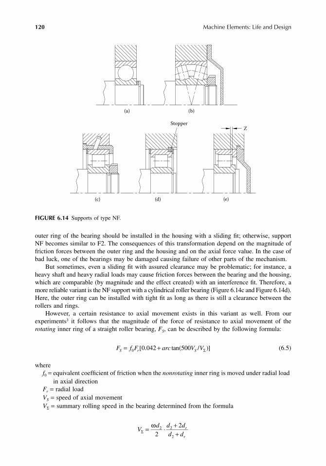
120 Machine Elements: Life and Design
outer ring of the bearing should be installed in the housing with a sliding fit; otherwise, supportNF becomes similar to F2. The consequences of this transformation depend on the magnitude offriction forces between the outer ring and the housing and on the axial force value. In the case ofbad luck, one of the bearings may be damaged causing failure of other parts of the mechanism.
But sometimes, even a sliding fit with assured clearance may be problematic; for instance, aheavy shaft and heavy radial loads may cause friction forces between the bearing and the housing,which are comparable (by magnitude and the effect created) with an interference fit. Therefore, amore reliable variant is the NF support with a cylindrical roller bearing (Figure 6.14c and Figure 6.14d).Here, the outer ring can be installed with tight fit as long as there is still a clearance between therollers and rings.
However, a certain resistance to axial movement exists in this variant as well. From ourexperiments3 it follows that the magnitude of the force of resistance to axial movement of therotating inner ring of a straight roller bearing, FS, can be described by the following formula:
(6.5)
wheref0 = equivalent coefficient of friction when the nonrotating inner ring is moved under radial load
in axial directionFr = radial loadVS = speed of axial movementVΣ = summary rolling speed in the bearing determined from the formula
FIGURE 6.14 Supports of type NF.
(a)
(c) (d) (e)
(b)
StopperZ
F f F arc V VS r S= +0 0 042 500[ . tan( / )]Σ
Vd d d
d dr
rΣ = ⋅ +
+ω 2 2
222
9563_C006.fm Page 120 Wednesday, July 25, 2007 4:17 PM

Supports and Bearings 121
ω = angular speed of the inner ring (rad/sec)d2 = inner race diameterdr = roller diameter
The experiments revealed decreasing f0 during running-in of the bearings. For example, aftera 10-h run under load, the friction coefficient decreased from 0.14 to 0.09. For practical calculations,it can be taken that f0 = 0.11.
In the same research, the axial force created by a straight roller bearing with an angularmisalignment of rings was measured. The magnitude of this force can be determined usingEquation 6.5, where
Hereγk = angle between the axes of the inner and outer ringsΘ = angle between the vector of radial load and the plane that passes through the axes of the rings
(Please be so kind as to present the angles in radians only, because degrees belong to the weatheras well, and you never know whether the forecast is true.)
According to the experiments, at VS/ VΣ < 0.0002 the resistance to axial movement of the ringbecomes negligible.
EXAMPLE 6.3
Cylindrical roller bearing NU310E, d = 50 mm, D = 110 mm, b = 27 mm, d2 = 65 mm, dr = 16 mm.Radial load Fr = 10,000 N, rotational speed n = 500 r/min. The shaft oscillates axially at thefrequency of rotation and with an amplitude of a = 0.1 mm. What is the axial force of resistance?
Maximum speed of axial movement of the shaft:
Next we find,
This is the maximum magnitude; the minimum is zero when the shaft passes the return points.The design shown in Figure 6.14e is used when the axial movement is relatively small. Gap Z
is installed to ensure the needed motion.
6.2.4 CHOICE AND ARRANGEMENT OF SUPPORTS
Let’s consider several options of laying out supports. Figure 6.15 shows the top view of a three-stage reduction gear (the cover is removed). Shafts 1, 2, and 3 have two supports of type F1 each.
V
VS
kΣ
Θ= 0 5. tan( sin )γ
ω π π= = ⋅ = = ⋅ ⋅ + ⋅−ns V
30500
3052 4
52 4 652
65 2 166
1. ;.
Σ 55 162038
+= mm s/
V a mm sS = = ⋅ =ω 0 1 52 4 5 24. . . /
V
V
F a
S
S
Σ
= =
= ⋅ +
5 242038
0 00257
0 11 10000 0 042
.. ;
. [ . rrc Ntan( . )]500 0 00257 1046⋅ =
9563_C006.fm Page 121 Wednesday, July 25, 2007 4:17 PM

122 Machine Elements: Life and Design
Such a design is the simplest. The inner rings of the RBs are mounted against the shoulders of theshaft. As a rule, no additional fastening of the inner rings but the tight fit is needed. End caps boltedto the gear housing restrict the possible motion of the outer rings. Shafts 1 and 2 don’t need exactaxial positioning, and their axial play is limited using shims 4 and 5 to within 0.5 to 1 mm.
If the gear reciprocates, as a travel mechanism of a crane does, every change in direction ofthe torque transmitted leads to axial displacement of the shafts within existing axial play. To decreaseimpacts and wear of the housing in such cases, the axial play is to be minimized.
The axial play of the shaft 3 tapered-roller support bearings needs to be precisely adjusted, andalso the shaft must be positioned axially so as to superpose the gear 5 cone vertex with the axisof pinion shaft 6. Therefore, shaft 6 is provided with two shims, 7 and 8, which first allowadjustment of the axial position of the shaft (for example, by changing the thickness of shim 7)and then that of the axial play of the bearings, using shim 8.
The design is more complicated when a combination of supports F2 + NF is used (compareshafts 1 and 2 in Figure 6.15 and their variants in Figure 6.16a and Figure 6.16b). In this case, thebearing installed in support F2 must be fixed relative to the shaft in both directions, and this requiresan additional component, such as nut or snap ring. The outer ring of this bearing also must be fixedin both directions relative to the housing, and for this purpose, additional components are required:cups, retaining rings, etc. Although complicated in design, which is certainly undesirable, thiscombination of types F2 + NF yields some important advantages. Influence of thermal and elasticdeformations on axial play is completely avoided, and axial positioning of the shaft neck adjoinedto the F2 support can be made as exact as needed. Furthermore, the misalignment of the shaftcaused by taking up the radial clearances unevenly (as shown in Figure 6.12) is avoided as well.
Support F2 of shaft 6 in Figure 6.15 is made up of two tapered roller bearings. Shim 9 isrequired to adjust the axial play of these bearings, and shim 10 to adjust the axial position of thebevel pinion so as to superpose the vertex of its base cone with the axis of shaft 3. This supportis designed according to Figure 6.8h, but it may be designed by variants shown in Figure 6.8e,Figure 6.8g, and Figure 6.8i as well. Other options from Figure 6.8 are not suitable for differentreasons: the support as in Figure 6.8a is not suitable for axial loads, and supports shown in Figure6.8b to Figure 6.8f don’t ensure the needed positioning precision because of increased axialmovement (see explanations in the preceding text).
FIGURE 6.15 Bearing arrangement in a three-stage gear.
415237
8
10
9
6
11
12
9563_C006.fm Page 122 Wednesday, July 25, 2007 4:17 PM

Supports and Bearings 123
The shaft depicted in Figure 6.16a represents a version of shaft 1 in Figure 6.15. In this version,a more durable cylindrical roller bearing is installed on the output-end side. Because this bearingis not designed for taking axial loads, this function is imposed on the ball bearing, which formssupport of type F2.
In the version shown in Figure 6.16b, in comparison with the shaft 2 in Figure 6.15, there isno need to adjust bearings, and owing to separate taking of radial and axial loads, possiblemisalignment of the shaft (such as depicted in Figure 6.12) is avoided. The design of supportsshown in Figure 6.16c and Figure 6.16d has been taken from aircraft reduction gears. Here, theaxial force is taken by a four-point ball bearing. Its outer ring is installed with a radial clearanceand can’t take any radial load.
6.2.5 FITS FOR BEARING SEATS
In operation, the inner ring of an RB is similar to a part of the shaft and should work as an integralpart of it. Similarly, the outer ring should be similar to an integral part of the housing. In otherwords, the connection of the bearing rings with the shaft and the housing should be as durable aspossible.
From this point of view, it would be ideal to use RBs without rings, produce raceways directlyon the shaft and in the housing, and put between them a set of rolling elements (balls or rollers)with or without a cage. This ideal, as are other ideals, is very costly or unattainable at all. Sometimes,when there is no place for the rings, ringless RBs are indeed used (see Subsection 6.2.8), but as arule, RBs are produced separately from the other parts of the mechanism. This allows productstandardization and mass production of RBs, which reduce their price by far. Besides, when theservice life of an RB is over, it can be easily replaced by a new one irrespective of the other parts.Therefore, even in aviation engineering, where reliability and decreasing weight are of paramountimportance, RBs are mostly used as separable units.
Generally, the connection of the rings with the shaft and the housing should prevent their turningrelative to the mating parts, because it may result in wear of the fitted surfaces. The main, and also
FIGURE 6.16 Bearing arrangement F2 + NF.
(c)
(a) (b)
(d)
9563_C006.fm Page 123 Wednesday, July 25, 2007 4:17 PM

124 Machine Elements: Life and Design
the cheapest, way to achieve this goal is to use interference fits. To define the magnitude ofinterference needed to prevent turning of the rings, the interaction between the ring and the adjoinedpart is considered. The mechanism of this interaction (as researchers from the Odessa PolytechnicUniversity have proposed it*) is as follows: If a cylindrical roller 1 presses on a strip 2 lying freelyon an elastic foundation 3 (see Figure 6.17a), the strip indents the foundation, and during theindentation, there occurs some sliding between them. The friction forces are symmetrical about thevertical axis of the roller and directed as shown in Figure 6.17a. If the roller is rolling (Figure 6.17b),the pressure between the strip and the foundation increases in front of the roller. Behind the roller,the pressure decreases, and the friction forces reverse their direction. In this way, all the frictionforces between the strip and the foundation, as well as the friction in rolling contact, act in thesame direction and move the strip relative to the foundation in the direction of rolling. As appliedto RBs, strip 2 is a ring of a bearing, elastic foundation 3 is a shaft or housing, and roller 1 is arolling element of a bearing.
The mechanism described in the preceding text provides an explanation for the well-knownphenomenon of turning of the stationary outer rings of RBs relative to the housing when slide-fitted. Similarly, the inner ring may turn relative to the shaft if it is fitted with insufficient interfer-ence. For an approximate determination of the interference magnitude needed to prevent turningof the ring, the friction in the rolling contact is neglected. With this assumption, the tangent forcemoving the ring may be estimated from a formula:
FIGURE 6.17 Interaction of rollers, ring, and shaft.
* Unfortunately, the authors didn’t succeed in establishing the names of the researchers. They are asked to send CRC Pressa copy of their article for reference in the following edition.
(a)
(b)
(c)
(d)
Gap
21
3
Fr
p
Fr
F F fm r C= ⋅
9563_C006.fm Page 124 Wednesday, July 25, 2007 4:17 PM

Supports and Bearings 125
whereFr = radial load on the rolling elementsfC = friction coefficient in the areas of interaction between the rolling elements, ring, and shaft
(or housing)
Circumferential friction force, which prevents the ring from moving, is estimated from theinterference fit:
wherep = surface pressure caused by the interference fitd = diameter of the mounting surface (say, the shaft neck)b = width of the ringfP = friction coefficient in the interference fit
Putting Fm equal to Fh and fC equal to fP , we obtain the needed minimal magnitude of thesurface pressure p:
(6.6)
The magnitude of the interference δ (that means the difference between the diameters of maleand female parts), which is required to achieve the needed pressure p, may be determined from anequation:4
(6.7)
(Here p is expressed in MPa, and d in mm.) and
whered1 = diameter of the central hole in the male part (shaft or outer ring of the bearing) (mm)d2 = outer diameter of the female part (inner ring of the bearing or boss of the housing) (mm)E1 and E2 = modulus of elasticity for the male and female parts, respectively (MPa)ν1 and ν2 = Poisson’s coefficients for the male and female parts, respectively
By the term 2C ⋅ p0.5, the increased compliance of the surface layer has been taken into account.It depends on the surface roughness. For the roughness height Ra = 1.25 µm, C = 1.4; for Ra = 0.63µm, C = 1.1; for Ra = 0.32 µm, C = 0.8.
EXAMPLE 6.4
Calculation of the interference required between the inner ring of the bearing and the shaft: Cylindricalroller bearing NU310E (d = 50 mm, b = 27 mm) is loaded with a radial force Fr = 10,000 N.
F p db fh P= π
pFdbr=
π
δ ξξ
ν ξξ
= ⋅ +−
−
+ +−
pdE E
101 1
11 1
13
1
12
12 1
2
22
222 2
0 52+
+ν µCp m.
ξ ξ11
22
= =dd
dd
;
9563_C006.fm Page 125 Wednesday, July 25, 2007 4:17 PM

126 Machine Elements: Life and Design
The needed pressure in the interference fit can be found from Equation 6.6:
Both the bearing ring and the shaft are made of steel, so E1 = E2 = 2.06 ⋅ 105 MPa, ν1 = ν2 = 0.3.The shaft doesn’t have a central hole, so d1 = 0 and ξ1 = 0. The outer diameter of the inner ringd2 = 65 mm, so ξ2 = 50/65 = 0.769. Roughness of the fitted surfaces Ra = 0.63 µm, so C = 1.1.Now we put all these values into Equation 6.7:
Thus, the minimum interference should be 6.2 µm. To fulfill this requirement, the m5 fit shouldbe chosen for the shaft. This fit gives interference within 9–32 µm.
Now, we have to check the bearing clearance in the case of maximum interference, which is32 µm. Increase in diameter of the inner raceway may be found as follows:
• First from Equation 6.7 can be found by iterations the pressure p at an interference of32 µm: p = 19 MPa.
• Then the increase of the inner raceway diameter d2 can be found using the Lame formula.
Radial clearance in this bearing before mounting (for normal clearance group) lies within30–60 µm. That means that even if the fit interference is maximal, the bearing clearance is still12.7 µm, at least.
There is another, old-stager explanation of the phenomenon of the turning of bearing ringsfitted with insufficient interference. Without a radial load, the pressure in the fit is distributed evenly(Figure 6.17c), but under load, the pressure in the loaded part increases, and on the opposite side,it decreases to the point of disappearance (Figure 6.17d).
Imagine that you have a ring on your finger sitting tight. But if you press on it in the radialdirection (especially from the inner side of the palm), on the opposite side, there will appear a gapbetween the ring and the finger.
If reality conforms to what is shown in Figure 6.17d, rotation of the shaft will certainly leadto turning of the ring relative to the shaft. Investigation has revealed5 that the minimum interferenceat which there is no gap between the ring and the shaft in the unloaded zone can be determinedfrom the equation
whereFr = radial load (N)b = width of the ring (mm)
p MPa=⋅ ⋅
=1000050 27
2 35π
.
δ = ⋅ ⋅⋅
+ +−
2 35 50 10
12 06 10
11 0 7691 0 769
35
2
2.
...
+ ⋅ ⋅ =2 1 1 2 35 6 2. . . µm
∆dd d p
E d d2
22
22 2
2
5 2
2 2 50 65 192 06 10 65
=−( ) = ⋅ ⋅ ⋅
⋅. ( −−= =
500 0173 17 3
2). .mm mµ
δ µ= 0 0043.Fb
mr
9563_C006.fm Page 126 Wednesday, July 25, 2007 4:17 PM

Supports and Bearings 127
Taking into account the roughness of the surfaces, geometrical errors, and the necessary factorof safety, the author of the investigation recommends increasing the interference more thanthreefold:
For bearing NU310E (from Example 6.3), the interference calculated by this formula should be
This result is close to what was obtained in Example 6.4 (6.2 µm), but Equation 6.6 andEquation 6.7 are more physical as they take into account real dimensions of the parts and roughnessof the contacting surfaces.
Not always can RBs be installed with interference that ensures a completely immovableconnection. For example, sometimes, it is desirable to use slide fit to make assembly anddismantling easier or to enable axial movement of the bearing relative to the housing to com-pensate for temperature expansion of the shaft. But what if the RB is fitted with a clearance?As experience shows, the behavior of the slide-fitted connections depends mostly on ring motionrelative to the radial load vector. If the ring rotates relative to the load vector (so-called circum-ferential load of the ring), the clearance connection will be soon damaged. Depending on thehardness of the shaft neck (or the housing socket), the rotational speed, and the load magnitude,there may be observed fretting, wear, scoring, and even local welding and tearing-out of metalparticles. But if the ring is nominally stationary relative to the load vector (point load), the ringwill slowly slip (creep) relative to the mating part. Thus, wear must certainly occur, but if themating part is made of wear-resistant material, the wear could be of low intensity and quiteacceptable for the needed service life. If the wear is too intense, the ring should be securedagainst slippage. (For example, the stopper in Figure 6.14d is put into a slot cut in the bearing’souter ring and in the housing. This stopper should be strong enough to take the tangential force,which is the product of radial load by friction coefficient, and to withstand wear, because thering is slightly moving.)
In most cases, the shaft with the inner ring rotates, and the radial load vector is constant indirection (for example, this condition exists for all bearings in Figure 6.15 and Figure 6.16). Thus,the inner rings are exposed to a circumferential load and the outer rings, to a point load. Underthese conditions, the inner ring should have interference-fit connection with the shaft, and for theouter rings, slide fit is acceptable. It is especially important because the housing is split throughthe axes of gears, and the interference fit here is impracticable.
In the cases shown in Figure 6.3, the load vector is also constant in direction, but the innerrings of the bearings are nominally stationary (point load) and the outer rings are rotating(circumferential load). Thus here, the outer rings should have a tight fit, and the inner rings canbe slide-fitted.
Another typical case is that of an eccentric weight attached to a rotating shaft (for example, inmechanical vibrators). Here, the inner rings of the bearings are exposed to a point load and theouter rings, to a circumferential load. Therefore, the inner rings may be slide-fitted, but the outerrings should be fitted tightly.
The slide fit for the “point-loaded” rings is only optional, and it is desirable to make it tighter.But the interference fit for the “circumferentially loaded” rings is mandatory, with very rareexceptions, which need special consideration.
δ µ= 0 0143.Fb
mr
δ µ= =0 014310000
275 3. . m
9563_C006.fm Page 127 Wednesday, July 25, 2007 4:17 PM

128 Machine Elements: Life and Design
On this basis, the designer should choose the fit taking into consideration the following:
1. Circumferentially loaded rings should be installed with interference fit. The minimalmagnitude of the interference may be determined using Equation 6.6 and Equation 6.7.
2. The interference should not be too much to keep a certain clearance in the bearing;bearings with increased clearance (C3 and C4) can be used when needed.
It is appropriate here to discuss the effect of clearances on the load capacity of RBs. Figure 6.18ashows the load distribution between the rolling elements under the assumption that before loadapplication, all clearances were zero. All rolling elements placed in the loaded half of the bearingtake part in the load transmission. If there was some initial clearance in the bearing (Figure 6.18b),some of the rolling elements (at the ends of the loaded half of the bearing) would not be able totransmit load because of the clearance. The neighboring elements come into contact, but they areloaded less than before, when the clearance was zero. And the rolling elements in the middle ofthe loaded area are overloaded. If there is a clearance between the bearing and the housing(Figure 6.18c), the outer ring is too pliable to transfer the radial load; it becomes elasticallydeformed, and the clearance of the fit has nearly the same effect as the internal clearance of thebearing.
So, it is desirable to keep the clearances as small as possible, and in the first place, by installingrings with a tight fit. In practice, there may be problems caused by different limitations. They canbe related to the assembly method, dismantling, or the requirement for free axial motion of a loosebearing, as mentioned in the preceding text. It is not recommended that considerable interferenceis used when the shaft neck is slotted or splined, because the initially round ring may becomepolygonal. In the latter case, the needed strength of the connection may be achieved by axialtightening with a nut (Figure 6.19a).
For the same reason (uneven deformation of the rings), a tight fit should be avoided whenmounting RBs into a split housing. If the outer ring in a split housing is loaded circumferentially,
FIGURE 6.18 Load distribution in a bearing.
Bearing
outer ring
Housing
Bearinginner ring
Bearing internal
clearance Clearance fit
(a)
(b) (c)
9563_C006.fm Page 128 Wednesday, July 25, 2007 4:17 PM

Supports and Bearings 129
it should be fixed additionally by axial tightening with bolts (Figure 6.19b), or it can be installedwith interference fit in a thick-walled sleeve (Figure 6.19c), which is in turn slide-fitted and boltedto the housing.
When using decreased bearing clearance, determination of temperature deformation andmachining of the parts must be performed with higher accuracy. Interference within the bearingmay lead to high contact stresses, which are greater than that from the working load. Therefore,prestressing (i.e., preloading) of RBs is used only for more exact positioning of the shafts, and notto increase their load capacity.
For prestressing, adjustable bearings are usually employed: angular contact ball bearings andtapered roller bearings (Figure 6.4b and Figure 6.4f). In these bearings, the prestress is appliedafter they have been mounted on the shaft and in the housing. So the tolerances of the fittingsurfaces don’t affect the prestress value, which may be adjusted independently and infinitely usingnuts, shims, or axial forces created by springs. The preferable arrangement of such bearings(especially when the shaft is overhanging) is shown in Figure 6.20a. It has two advantages:
• Better ratio between bearing spacing L and overhanging length C.• When the bearings are prestressed, thermal expansion of the shaft in axial and radial
directions compensate each other, so that the prestress doesn’t change a lot. In the designshown in Figure 16.20b, both the radial and the axial expansions of the shaft sum upand increase the initial prestress.
The ring exposed to a point load may be installed with a tight fit or a sliding fit. The latter isneeded for some supports of type NF (as in Figure 6.14a and Figure 6.14b) and in cases where thebearing can’t be tightly fitted (some of them have been discussed in the preceding text).
Possibly you ask yourself: who needs all these complicated things, all these formulas? Inall catalogs, we can find recommendations on how to choose bearing fits, depending on thetype of the bearing, mode of load, and load level. Perhaps they are false? God forbid! Thecatalog recommendations are perfectly right, but sometimes not detailed enough. For example,the scale of load levels often looks as follows: low load, normal load, high load, and high loadwith shocks. It is reasonable that designers dealing with, for example, ship gears (30,000 hservice life), helicopter gears (500 h), and racing motorcycle gears (designed for only one lap)have different ideas about what is normal load. Besides, short-term overloads may occur inservice, associated with planned tests or with emergency operation. They don’t influence theservice life of the bearings (as long as the loads don’t exceed the permitted static load), and itis not clear whether they should be taken into account while choosing the bearing fits. Let’sconsider one practical case.
FIGURE 6.19 Fastening of bearing rings.
(a) (b) (c)
9563_C006.fm Page 129 Wednesday, July 25, 2007 4:17 PM

130 Machine Elements: Life and Design
EXAMPLE 6.5
The main shaft of the escalator presented in Figure 4.20 and Figure 4.21 (see Chapter 4) rotatesin two spherical roller bearings 23056 with dimensions d = 280 mm, D = 420 mm, and b =106 mm. The radial load on the bearing near the gear is about 35 ⋅ 104 N, and on the otherbearing, 30 ⋅ 104 N. Twice a year, a test of the emergency brake is performed, and during thetest, the radial load of the latter bearing comes up (for several turns of the shaft) to 50 ⋅ 104 N.Of course, this overload has not been taken into account when calculating the service life ofthe bearings.
Angular speed of the shaft n = 11.2 r/min, loading rating (dynamic) C = 1.56 ⋅ 106 N, and forthe radial load of 35 ⋅ 104 N, it was found, L = 200,000 h. The escalator is in service about 20 ha day, 300 d a year; thus, the service life is more than 30 years. When choosing the fit, the designerhad opened the manufacturer’s recommendations and started to think over the load level: is itnormal or high with shocks. If you were going by escalator, you would just feel that there are noshocks. And taking into account the enormous service life, you can’t say that the load is heavy!It is low, or normal. For the normal load, the recommended fit is m6, which results in interferenceof 20 µm minimum and 87 µm maximum. This fit was chosen by the designer. And then theescalator was built, installed in the metro station, and tested. When testing the emergency brake,it was revealed that the inner ring of the bearing turns relative to the shaft neck. The shaft is madeof mild steel, so the relative motion would be able to wear out the neck very soon. The way outof this situation was found in additional axial fastening of the bearing by an end washer withplenty of bolts. (Imagine what a pleasure it was to machine all these dozens of threaded holes onthe shaft by hand tools!)
FIGURE 6.20 Arrangement of tapered roller bearings.
L
L
C
Prefearable
(a)
Not as good
(b)
9563_C006.fm Page 130 Wednesday, July 25, 2007 4:17 PM
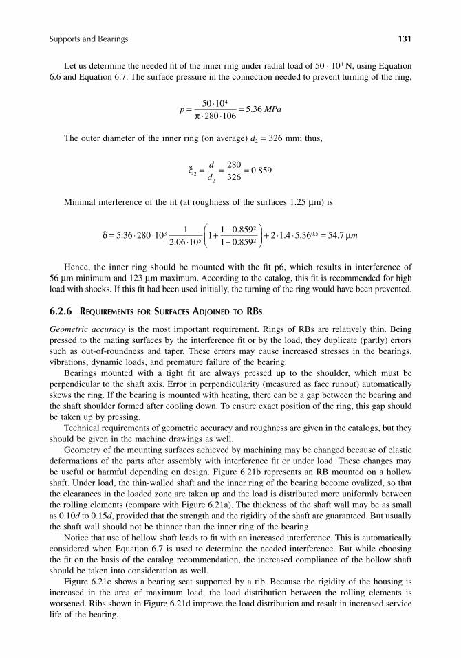
Supports and Bearings 131
Let us determine the needed fit of the inner ring under radial load of 50 ⋅ 104 N, using Equation6.6 and Equation 6.7. The surface pressure in the connection needed to prevent turning of the ring,
The outer diameter of the inner ring (on average) d2 = 326 mm; thus,
Minimal interference of the fit (at roughness of the surfaces 1.25 µm) is
Hence, the inner ring should be mounted with the fit p6, which results in interference of56 µm minimum and 123 µm maximum. According to the catalog, this fit is recommended for highload with shocks. If this fit had been used initially, the turning of the ring would have been prevented.
6.2.6 REQUIREMENTS FOR SURFACES ADJOINED TO RBS
Geometric accuracy is the most important requirement. Rings of RBs are relatively thin. Beingpressed to the mating surfaces by the interference fit or by the load, they duplicate (partly) errorssuch as out-of-roundness and taper. These errors may cause increased stresses in the bearings,vibrations, dynamic loads, and premature failure of the bearing.
Bearings mounted with a tight fit are always pressed up to the shoulder, which must beperpendicular to the shaft axis. Error in perpendicularity (measured as face runout) automaticallyskews the ring. If the bearing is mounted with heating, there can be a gap between the bearing andthe shaft shoulder formed after cooling down. To ensure exact position of the ring, this gap shouldbe taken up by pressing.
Technical requirements of geometric accuracy and roughness are given in the catalogs, but theyshould be given in the machine drawings as well.
Geometry of the mounting surfaces achieved by machining may be changed because of elasticdeformations of the parts after assembly with interference fit or under load. These changes maybe useful or harmful depending on design. Figure 6.21b represents an RB mounted on a hollowshaft. Under load, the thin-walled shaft and the inner ring of the bearing become ovalized, so thatthe clearances in the loaded zone are taken up and the load is distributed more uniformly betweenthe rolling elements (compare with Figure 6.21a). The thickness of the shaft wall may be as smallas 0.10d to 0.15d, provided that the strength and the rigidity of the shaft are guaranteed. But usuallythe shaft wall should not be thinner than the inner ring of the bearing.
Notice that use of hollow shaft leads to fit with an increased interference. This is automaticallyconsidered when Equation 6.7 is used to determine the needed interference. But while choosingthe fit on the basis of the catalog recommendation, the increased compliance of the hollow shaftshould be taken into consideration as well.
Figure 6.21c shows a bearing seat supported by a rib. Because the rigidity of the housing isincreased in the area of maximum load, the load distribution between the rolling elements isworsened. Ribs shown in Figure 6.21d improve the load distribution and result in increased servicelife of the bearing.
p MPa= ⋅⋅ ⋅
=50 10280 106
5 364
π.
ξ22
280326
0 859= = =dd
.
δ = ⋅ ⋅⋅
+ +−
5 36 280 101
2 06 101
1 0 8591 0 859
35
2
2.
...
+ ⋅ ⋅ =2 1 4 5 36 54 70 5. . .. µm
9563_C006.fm Page 131 Wednesday, July 25, 2007 4:17 PM

132 Machine Elements: Life and Design
Strength and wear resistance of the surfaces adjoined to the RBs are of secondary importanceif the connection between the bearing ring and the seat is motionless. This immobility should beensured not only at normal conditions, but also while starting, on trials, in emergency operation withoverload and vibrations (because of out-of-balance), and so on. If the wear resistance of the shaftis low, even momentary turning of the bearing ring about the shaft neck may decrease the interferenceand result in distortion of the connection. That’s why it is advisable to ensure wear resistance of RBseats. Sometimes, the shaft necks are surface-hardened by carburizing or nitriding, especially whenthis surface treatment is needed for the strength of the shaft itself or of other elements such as splines,gear teeth, cams, etc. But, usually, there is no need for surface hardening. When the bearing ring isslide-fitted, the wear resistance of the surfaces is of primary importance. Seats in light metal housingsshould be shielded with sleeves made of heat-treated steel. The sleeves are press-fitted into thehousing so as to retain the interference fit despite the greater expansion of the housing under workingtemperature. Additionally, the sleeves are usually fixed with pins or bolts (Figure 6.14c, Figure 6.16c,and Figure 6.16d). Holes for the pins are drilled after the sleeves are installed in place.
The height of the shaft shoulders may be important, particularly when the shoulder transmitsan axial force from the bearing (when using tapered roller bearings, this force can be created as acomponent of radial load). The authors have seen shoulders worn out in contact with a commonball bearing. If the bearings are of adjustable type (such as angular contact ball bearings or taperedroller bearings), the gradual wear of the shoulders increases their axial play and leads to increasingradial displacement of the shaft. High wear resistance is needed not only for the shaft shoulders,but also for support elements that fix the bearing ring axially: end cups, spacers, shims, etc.
The designer is interested in making the shaft shoulder height as small as possible; it enablesdecreasing of the shaft diameter and reduces stress concentration. However, there can be negativeconsequences of decreasing the shoulder height, as illustrated by the following bitter experience.
FIGURE 6.21 Flexibility of shaft and housing and load distribution in the bearing.
Hollow shaft
(a) (b)
(c) (d)
Ribs
Rib
9563_C006.fm Page 132 Wednesday, July 25, 2007 4:17 PM

Supports and Bearings 133
EXAMPLE 6.6
In Figure 6.22 is shown the output shaft assembly of a reduction gear. The designer was aspiringto decrease the diameter and the cost of the shaft. Diameters d1 and d3 can’t be decreased, becausethey are limited by the strength of the shaft. Diameter d2 serves as a shoulder for the gear and theright-hand bearing. The shoulder height is dictated by the bearing catalog recommendations, butthere is a well-known ruse: the shoulder can be made small, but between it and the bearing a spacerring can be installed, which has the height as recommended by the catalog. This method is excellenton condition that the compressive resistance of the small shoulder is sufficient to take the axialforces originated from the load transferred by a mechanism. This aspect was not taken intoconsideration in this case. The designer didn’t find a suitable steel tube for sleeve 1, so he madeit of low-quality gray iron. In operation, the axial force is not distributed uniformly over the entirecircumference, but concentrated on a part of it (see Figure 6.13c). Taking into account that themaximal radial load on a rolling element is given by
where z is the number of rolling elements in the bearing, it can be assumed that the load concen-tration factor is about 5 in the axial direction as well. This loaded area in contact between sleeveand shoulder moves circumferentially with the shaft rotation speed. Sleeve 1 was mounted on theshaft with a clearance, so its motion relative to the shaft shoulder was unhindered. This cyclicloading resulted in wear and squash of the contacting surfaces 2, which became tapered. After that,sleeve 1 cracked along its generatrix, moved toward the gear (together with the bearing, certainly)and got on the d2 part of the shaft. The shaft became terribly skewed, and severe noise and vibrationin the gear suggested to the maintenance staff that something must be wrong with it. For the renewal,a new shaft was made, with increased diameter between the gear and the bearing, d2, without anysleeve. The gear and the pinion were replaced as well, because they were severely damaged. Inshort, this is a story about unlucky economization. As they say, “the stingy pay twice.”
6.2.7 ELASTIC DEFORMATION OF RBS UNDER LOAD
As was already said, the possible movement of the shaft in the support involves clearances in thebearing and in the fits, resilience of the bearing, and housing deformation where the bearing isinstalled. In this section, we will study the resilience of the bearings, which consists mostly ofdeformation where rolling elements contact the rings (δ1), and also includes deformation of thehousing (δ2) and the shaft (δ3) under tight fits. Deformations of the bearings have been investigatedin detail. In the following text are given simplified formulas to calculate them.4
FIGURE 6.22 Height of the shaft shoulder.
RR
zmax cos≈ 5
β
d3
1
d2 d1
2
9563_C006.fm Page 133 Wednesday, July 25, 2007 4:17 PM

134 Machine Elements: Life and Design
For approximate determination of δ1, the following averaged equations can be used. For single-row ball bearings:
(6.8)
For roller bearings:
(6.9)
HereFr = radial load of the bearing (N)kb, kr = factors that depend on type and size of bearing
For bearings with inner diameter d of 40–100 mm, the factors k are as follows:
• Single-row ball bearings: kb = 0.153–0.00044d• Regular tapered roller bearings: kr = 0.052/d• Wide tapered roller bearings: kr = 0.033/d• Regular straight roller bearings: kr = 0.065/d• Wide straight roller bearings: kr = 0.043/d
(Here, d shall be substituted in millimeters.)These formulas are correct when the initial (before loading) clearance in the bearing is zero.
If there is an initial clearance, a lesser number of rolling elements will take the load, and theirdeformation will increase. In the case of preload, the result will be opposite. The recommendedmethod of taking the clearance or the preload into account is as follows:
• If the ratio of the initial clearance (after the bearing is mounted on the shaft) to defor-mation δ1 rated from Equation 6.8 and Equation 6.9 is 1:1, 2:1, or 4:1, δ1 shall beincreased by 10, 20, or 30%, correspondingly.
• If the bearing is preloaded, its deformation δ1 should be divided for roller bearings by2–2.5 and for ball bearings by 2–5, depending on the preload magnitude.
The resilience of the tightly fitted connections (δ2 and δ3) is relatively small. In total they cometo 25–30% of δ1 for roller bearings and 20–25% of δ1 for ball bearings.
EXAMPLE 6.7
It is desired to define radial deformation of a straight roller bearing NU310E loaded with a radialforce R = 10,000 N. The bearing is mounted on a shaft with a tight fit m5, and the internal clearanceas mounted measures 12.7–42.7 µm (see Example 6.4).
Coefficient kr = 0.065/d = 0.065/50 = 0.0013
From Equation 6.9, deformation of a bearing with zero clearance,
δ1 = 0.0013⋅10,000 = 13 µm
The ratio of the internal clearance to δ1 equals 0.98 at a smaller clearance and 3.28 at a greaterone. Hence, the calculated deformation should be increased by 10 and 26%, correspondingly.
δ µ12 3= k F mb r
/
δ µ1 = k F mr r
9563_C006.fm Page 134 Wednesday, July 25, 2007 4:17 PM
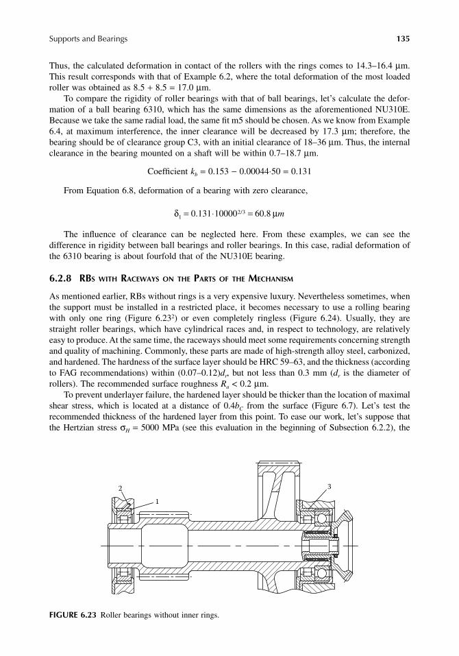
Supports and Bearings 135
Thus, the calculated deformation in contact of the rollers with the rings comes to 14.3–16.4 µm.This result corresponds with that of Example 6.2, where the total deformation of the most loadedroller was obtained as 8.5 + 8.5 = 17.0 µm.
To compare the rigidity of roller bearings with that of ball bearings, let’s calculate the defor-mation of a ball bearing 6310, which has the same dimensions as the aforementioned NU310E.Because we take the same radial load, the same fit m5 should be chosen. As we know from Example6.4, at maximum interference, the inner clearance will be decreased by 17.3 µm; therefore, thebearing should be of clearance group C3, with an initial clearance of 18–36 µm. Thus, the internalclearance in the bearing mounted on a shaft will be within 0.7–18.7 µm.
Coefficient kb = 0.153 − 0.00044⋅50 = 0.131
From Equation 6.8, deformation of a bearing with zero clearance,
The influence of clearance can be neglected here. From these examples, we can see thedifference in rigidity between ball bearings and roller bearings. In this case, radial deformation ofthe 6310 bearing is about fourfold that of the NU310E bearing.
6.2.8 RBS WITH RACEWAYS ON THE PARTS OF THE MECHANISM
As mentioned earlier, RBs without rings is a very expensive luxury. Nevertheless sometimes, whenthe support must be installed in a restricted place, it becomes necessary to use a rolling bearingwith only one ring (Figure 6.232) or even completely ringless (Figure 6.24). Usually, they arestraight roller bearings, which have cylindrical races and, in respect to technology, are relativelyeasy to produce. At the same time, the raceways should meet some requirements concerning strengthand quality of machining. Commonly, these parts are made of high-strength alloy steel, carbonized,and hardened. The hardness of the surface layer should be HRC 59–63, and the thickness (accordingto FAG recommendations) within (0.07–0.12)dr, but not less than 0.3 mm (dr is the diameter ofrollers). The recommended surface roughness Ra < 0.2 µm.
To prevent underlayer failure, the hardened layer should be thicker than the location of maximalshear stress, which is located at a distance of 0.4bC from the surface (Figure 6.7). Let’s test therecommended thickness of the hardened layer from this point. To ease our work, let’s suppose thatthe Hertzian stress σH = 5000 MPa (see this evaluation in the beginning of Subsection 6.2.2), the
FIGURE 6.23 Roller bearings without inner rings.
δ µ12 30 131 10000 60 8= ⋅ =. ./ m
2
1
3
9563_C006.fm Page 135 Wednesday, July 25, 2007 4:17 PM

136 Machine Elements: Life and Design
length of the roller L = 1 mm, and the roller contacts a flat surface (in this case, re = 0.5dr). Now,from Equation 6.2 we can obtain the force F:
The width of the contact area is obtained from Equation 6.3:
As we can see, the recommended thickness of the hardened layer approximately equals thewidth, bC, of the contact area, i.e., 2.5 times deeper than the location of the maximal shear stress.
It should be noticed that the part containing the raceways may also have other elements limitingthe thickness of the hardened layer. For example, gear teeth need the carbonization depth to be(0.28–0.007m) m ± 0.2 mm plus grinding allowance.
(Here, m is the module of the gear, in mm. In the American system of terms,
where P is the diametral pitch.The carbonization depth is uniform on all surfaces of a part, and it should be suitable to all
‘‘interested parties.”Figure 6.23 shows a double-geared shaft with a bevel gear attached to it. It has one NF support
(straight roller bearing without inner ring) and one F2 support. The F2 includes an identical rollerbearing and a four-point ball bearing, the latter taking only the axial force generated in the gears.The inner raceways of the roller bearings are made directly on the shaft ends. A bearing manufacturersupplies the outer rings with a set of rollers and a cage.
In supports depicted in Figure 6.24, rollers 1 are the only parts received from a bearingmanufacturer, and the manufacturer of the gear makes the rest. Support of a planet wheel as shown
FIGURE 6.24 Self-made roller bearings.
(a)
15
16
Oil inlet Oil inlet
(b)
3
6
1
2
4 5
7
8
9
11
1
14 12
10
13
18
17
19
Fr L
EdH e r= = ⋅ ⋅
⋅ ⋅σ2
2
2
2 50 4185000 0 5
0 418 2 06 10..
. .== 347 3. /d N mmr
bd d
d mmCr r
r= ⋅ ⋅ ⋅⋅
=3 04347 3 0 5
2 06 100 088
5.
. ..
.
mP
mm= 25 4.
9563_C006.fm Page 136 Wednesday, July 25, 2007 4:17 PM

Supports and Bearings 137
in Figure 6.24a is classic. Planet wheel 2 runs on two rows of rollers that are separated by rings 3and 4. Two rings 5 fixed by snap rings prevent the axial motion of the planet wheel. Cage 6 iscentered by the middle ring 3. Lubrication oil enters the unloaded part of the bearing through holesin axle 7. The oil ducts are organized in such a way, that if there is some solid particle 8 in theoil, it will be separated by centrifugal forces and will remain in the labyrinth of insert 9. Axle 7should be safely fixed against rotation to keep the oil ducts in the axle and in planet carrier 10aligned. The oil flows out of the planet wheel through holes 11.
The planet wheel support shown in Figure 6.24a is formed, in effect, by a single two-rowcylindrical roller bearing. Axle 7 and two rings 4 form (together with planet carrier 10) the innerring with two lips. The outer ring with two lips is formed by planet wheel 2 and two rings 5. Ring3 serves as a floating center lip that separates two rows of rollers.
Rings 3, 4, and 5 can be made of high-carbon low-alloy steel as usual for rolling bearings. Butthe planet wheel 2, and axle 7, must not be brittle, so they should be made of low-carbon alloysteel. They should be case-hardened to obtain a hard surface layer while the core remains tough.All the surfaces contacting with the rollers should be case-hardened or carbonitrided, heat-treatedto high hardness, and then thoroughly ground and polished.
Planet wheel 12 shown in Figure 6.24b works at lower speeds, and the design of its support isuncommon. Seven rows of rollers 1, without a cage (so-called ‘‘full complement design”), areseparated by hardened rings 13. Between the planet wheel and planet carrier 14 are placed hardenedrings 15 with antifriction coating, which are able to take relatively small axial forces from the spurplanet wheel and the rollers. The oil is supplied through hole 16 in the planet carrier, and thenthrough oil ducts in axle 17. It flows out of the bearing through slots 18 made in thrust rings 15.
Thrust rings 15 are fixed against rotation to prevent the wear of the planet carrier. Axle 17 isfixed against axial movement and rotation by strip 19, which is bolted both to the axle and theplanet carrier.
6.2.9 LUBRICATION OF RBS
Detailed recommendations for rolling bearing lubrication are given in the manufacturers’ catalogs.It is noteworthy that when the speed is not high, the RBs are somewhat sensitive to lubricationgrade and mode. The main concern is not to leave the bearing without lubrication at all. Scarcity(or even worse, complete absence) of lubricant may lead to overheating and wear of all bearingelements, and seizure and breaking down of the cage.
It is important to prevent entrance of foreign matter (wear products from inside, dirt, and water)into the lubricant. For this reason, rubbing parts of the mechanism should be made wear resistantby means of hardening and proper lubrication of friction surfaces. The mechanism should besatisfactorily sealed from the surroundings. For trapping of ferromagnetic particles, magnetic plugsare in common use. In spite of this, some amount of foreign particles and products of oil decom-position accumulate in the lubricant bit by bit. When the speed is not too high, these impuritiesincrease the wear of RBs, but not drastically. Therefore, it is common to bear with small amountsof pollution in the lubricant, and not to complicate the mechanism by a circulation lubricationsystem with filters. At high speed, the lubrication oil should be filtered.
When choosing the lubrication mode, speed and temperature should be taken into consideration.Oil, as compared with grease, provides better heat removal and enables higher rotational speed.Decomposition of the oil proceeds more slowly, and it can be easily replaced. Oil can work atwide-ranging temperatures.
The main advantage of grease lubrication is that the grease doesn’t flow out; it makes thesealing problem much easier. In many cases, when the load and speed are moderate, sealed bearingsgreased for life can be used. Recommendations for the selection of suitable grease and lubricationintervals are given in bearing catalogs. When replenishing grease, don’t forget that the new greasemust be compatible with the previous formulation.
9563_C006.fm Page 137 Wednesday, July 25, 2007 4:17 PM

138 Machine Elements: Life and Design
When adjacent machine parts are lubricated with oil, it is practical to supply the oil to the RBsas well. It should be always checked whether there is a really sufficient supply of oil to the bearing.Sometimes, the bearing may remain dry in the middle of an oil storm, where apparently no dryplace could be found. Some information about this issue is given in Chapter 7, Section 7.10.
6.3 SLIDING BEARINGS (SBs)
6.3.1 FRICTION OF LUBRICATED SURFACES
The main problem to be solved when designing an SB is the decrease of friction forces. There maybe several modes of friction: liquid friction, semiliquid friction, and boundary friction. The modeof friction depends on many parameters, such as sliding velocity, unit pressure, temperature in thecontact area, geometry of the surfaces, and the properties of the lubricant. Among the immensevariety of SBs made of metals, rubbers, plastics, or wood and lubricated with oil, grease, water,air, or whatever else, we choose for consideration only the metal bearings lubricated with mineral oil.
The surface of a metal is remarkable for its molecular activity, because the atoms on the surfacedon’t have a full complement of atomic bonds (similar to the atoms inside crystals), and theyproduce atomic (molecular) attraction. This effect was described in the beginning of Chapter 3.Because of this attraction, the surface of the metal is “sticky,” and it is always covered with a verythin film of substances that have come in contact with it. This phenomenon is called adsorption.
In particular, because cutting emulsions are used in machining, in the beginning, the filmadsorbed on a part consists of molecules of oil, water, and gases. This film may be completelyremoved only by heating the part in a vacuum, but the composition of the film may be changed ifsubstances with greater surface activity (and, correspondingly, with greater ability of adsorption)are applied to the metal surface.
A distinctive feature of surface-active substances is that in their molecules the centers of thepositive and the negative charges don’t coincide.6 In other words, each of their molecules containstwo charges, positive and negative, separated in space. Such molecules, when they come in contactwith a metal, fasten onto its surface in a fixed manner (perpendicular to the metal surface, Figure 6.25)and create a monolayer 1 of one molecule thick. Lubrication oils containing surface-active additivescreate a boundary layer 2 over the monolayer 1, in which the molecules are also oriented perpendicular
FIGURE 6.25 Adsorbed oil film.
2
Metal
Oil
1
9563_C006.fm Page 138 Wednesday, July 25, 2007 4:17 PM

Supports and Bearings 139
to the metal surface. This layer has a quasi-crystal structure and is able to take very high loads, upto 3000 MPa. But under increased temperatures, the molecular links become weaker and the quasi-crystal layer “melts.” These temperatures for different metals lie in the range of 90–150°C.
Two surfaces contact first at microasperities on the top of the macrowaves (Figure 6.26a). As theload increases, the microasperities, and afterward the macrowaves, become deformed elastically andplastically, and thus the contact area grows with increased load. However, this area rarely exceeds30–40% of the nominal contact area. When there is no relative motion, the surfaces are separated (atpoints of closest approach) by a quasi-crystal boundary layer of oil, about 0.1 µm thick. When inmotion, sliding takes place between the boundary layers. Where the surfaces are close, there may bemechanical interaction and deformation of the surface asperities, with no damage to the boundary layer.Under certain conditions, the heat generated in spots of close contact may “melt” the quasi-crystalboundary layer. Then, in these spots may occur direct contact of metal surfaces, accompanied by localadhesion and seizing (microwelding) (see Figure 6.26b). But in the main, the sliding surfaces areseparated by the oil film, which is renewed in the spots where it was destroyed after the local conditionsimprove (while sliding). This described mode of friction is called boundary friction. The coefficientof friction and wear intensity in this mode are small as compared to dry friction (without lubrication).
It is clear that the better the actual fit of the sliding surfaces, the less the unit load in the spotsof close contact, and consequently, the risk of boundary layer destruction is less. Better fit is favoredby more exact geometry of the surfaces, smoother surface (in the first place, of the harder member),and lesser modulus of elasticity. From this point of view, rubber is a very good material, but inmost cases, it is too pliable to ensure the needed exact position of the shaft relative to the housing.(Propeller shaft bearings in boats and ships are a popular application for rubber bearings. They arealso used in hydroelectric power plant turbines).
Liquid friction is characterized by a complete separation of the surfaces by an oil film underpressure. In other words, the load, which presses the surfaces against each other, is supported notbecause of the mechanical strength of the adsorbed boundary layer, but rather, the pressure in theoil film. This pressure may be produced either by a special pump, which forces the oil betweenthe sliding surfaces (such bearings are called hydrostatic), or owing to the shape of the slidingsurfaces, which forms an oil wedge while sliding (such bearings are called hydrodynamic).
Oil layers placed at a distance of more than 0.5 µm from the metal surface (beyond the boundarylayer) may move freely relative to each other, and their resistance to movement is minimal. Thisfriction mode is the best with respect to minimizing friction and wear.
FIGURE 6.26 Contact of lubricated surfaces.
(a)
(b)
9563_C006.fm Page 139 Wednesday, July 25, 2007 4:17 PM

140 Machine Elements: Life and Design
Semiliquid friction constitutes a mixture of liquid and boundary modes. In hydrodynamicbearings, the percentage of each mode depends on load magnitude, sliding velocity, oil viscosity,and other factors. For example, an ordinary radial SB starts with boundary friction. As the slidingvelocity increases, the load capacity of the oil wedge grows, and the percentage of the liquid frictionincreases correspondingly. When the oil wedge is able to take the entire load, the surfaces arecompletely separated by an oil film, and the friction losses are minimal. Further increase of thesliding velocity leads to gradual increase in the friction coefficient, because the oil film thicknessgrows much less than the velocity does, and the velocity gradient within the oil film grows.
The process of transition from boundary friction through the semifluid to the fluid friction modeis reflected in the well-known diagram shown in Figure 6.27, in which is given the coefficient of frictionf vs. parameter ηv/q (η: oil viscosity, v: sliding velocity, q: unit load). Pure liquid friction is achievedwhen the f magnitude is minimal. On the left side of this point is semiliquid and boundary friction.
In hydrostatic SBs, pressure can always be produced, which is enough to bear the entire loadand completely separate the sliding surfaces. In hydrodynamic bearings, this possibility depends,among other parameters, on the sliding velocity, which inevitably begins at zero, when no hydro-dynamic effect can be gained. Therefore, in many cases, especially at start or shutdown of themachine, semiliquid and boundary friction modes are a matter of fact. Hydrostatic bearings areused relatively seldom, and so they will not be discussed further.
6.3.2 TYPES OF SBS
Routine design of supports with SBs is depicted in Figure 6.28: types NF (Figure 6.28a), F1(Figure 6.28b), and F2 (Figure 6.28c). In contrast to RBs, which may take both radial and axial
FIGURE 6.27 Hersey–Stribeck diagram.
FIGURE 6.28 Types of sliding bearings.
f
η v/q
(a)
S
(b) (c)
3
14
5 2
6
9563_C006.fm Page 140 Wednesday, July 25, 2007 4:17 PM

Supports and Bearings 141
forces, sliding bearings can take either radial or axial load but not both. Physically, both of themmay be combined into one, as shown in Figure 6.28c and Figure 6.28d, but their design andcalculation are completely independent.
They are designed independently, but often they live in close neighborhood and, as in real life,one flat mate can cause troubles for another. For example, thrust bearing 1 is lubricated with oilflowing out of radial bearing 2 into a circular chamber 3 (Figure 6.28b). If small particles of metalbreak away from the radial bearing (caused, for example, by wear or local submelting of theantifriction layer), these particles are transferred with the oil to the thrust bearing and may damageit. Being damaged (or wrongly designed), the thrust bearing may close the oil outlet from chamber 3.This leads to decrease of oil flow through the radial bearing, which may result in overheating andfailure.
As already mentioned, the necessary condition for continuous duty of SBs is the creation ofan oil film between the shaft journal and the bearing. If there is a wedge-shaped clearance betweenthese surfaces, which is opened toward the motion (Figure 6.29), the oil is pulled into this clearanceby friction. The oil then produces hydrodynamic forces, which tend to increase this clearancefurther. These forces are larger when speed or oil viscosity is greater. Because heat generated in asliding bearing decreases oil viscosity and reduces oil-film thickness, it is important to ensuresufficient heat removal. The most effective method is to increase oil circulation through the bearing,which can be accomplished by increasing the bearing clearance and the input oil pressure. Some-times, additional oil grooves are made to supply more chilled oil into the bearing.
The wedge-shaped clearance can be created by various means. In radial SBs, it arises automat-ically when the shaft becomes eccentric about the bearing under radial load (Figure 6.29a). In thrustbearings, this purpose may be served either by machining of the bearing surfaces with needed slope(Figure 6.29b) or by using floating elements (Figure 6.29c). When the load and the speed are low,thrust bearings with flat surfaces are used.
Radial clearance in a radial SB, as well as the wedge angles and clearances in thrust SBs, areshown exaggeratedly in Figure 6.29. In reality, the radial clearance measures 0.1–0.3% of the shaftdiameter, and the minimum oil-film thickness h measures microns or, at the most, tens of microns.The inclination angle of the thrust bearing surfaces is also very small. The opening of the wedget = (0.8–1.6)h, so it is a question of tens of microns as well. We will discuss this in the following text.
6.3.3 MATERIALS USED IN SBS
The journal of a shaft is typically made of steel. It may also have a hard metal coating, such aschrome. What is subject to discussion is the material of the bearing or, to put it more precisely, ofthe working surface, which is directly in contact with the shaft journal. Theoretically, if an oil filmseparates the bearing and the journal, it doesn’t matter what kind of material they are made from,
FIGURE 6.29 Formation of hydrodynamic oil film in sliding bearings.
h
(a)
g
a
(b) (c)
h t
Oil groove
tS
L
h
B
9563_C006.fm Page 141 Wednesday, July 25, 2007 4:17 PM

142 Machine Elements: Life and Design
if its thermal conductivity is high enough to ensure good heat dissipation. But the problem is thatthese surfaces are not always separated. When the mechanism is standing, the adsorbed oil layerseparates the surfaces of journal and bearing. When put into operation, the boundary friction maybe accompanied by local destruction of the boundary layer and direct contact of the two surfacesin local spots. The oil film sufficient for complete separation of the bearing and journal surfacesdoesn’t arise immediately. It takes several turns until the oil film becomes thick enough. Heavymachines, to prevent bearing damage during the start, are often provided with special devicesenabling filling out the lubrication system and the bearings with heated oil and slow rotation ofthe shafts before the load start. Afterward, the machine is put in operation and loaded gradually.In smaller machines, the process of putting in operation is certainly not so intricate. But anyway,during the first turns of the shaft, the microasperities of the journal and the bearing may not beseparated. This leads to some wear or, under adverse conditions, the damage may be more serious.
Direct contact in SBs may occur in operation as well. Occasional overloading of the bearing,local overheating, insufficient oil supply, and other conditions may cause this. It is clear that insuch cases, when two surfaces come into contact at high speed, the nature and extent of the damagedepend very much on the properties of the contacting materials.
Failures of SBs are usually caused by some abnormality, such as:
• Lack of, or low pressure of, oil• Contaminated oil• Overload caused by work under emergency conditions• Local overload due to inaccuracy of machining or assembly• Local overload due to elastic deformations of the shaft and the support under load
Against lack of oil or its contamination, nothing can help. The same can be said about emergencyconditions, but these cases are rare. What always exists is the local overload, and it is highlydesirable to impart to the SB the ability to somehow repair this problem by itself — some kind oflocal self-alignment. Therefore, the most important properties of the antifriction layer of the SBsare as follows:
Low hardness, which imparts to the bearing the ability to run in: As was said in the precedingtext, the minimal thickness of the oil film in SBs is measured in microns or tens of microns.Therefore, uneven load distribution, caused by corrugation and roughness of the surfacesand by misalignments of all kinds, may lead to local overload, overheating, and destructionof the oil film. Soft material may be easily plastically deformed, worn out, or even meltedin this small area, so that a minute amount of material is removed, the local load isdecreased, and the proper functioning of the bearing is restored.
Low melting temperature: Quick melting of the overloaded and overheated local spots ofthe bearing and subsequent better distribution of the load may prevent overheating anddamage of the entire bearing. The melted particles of bearing material are carried out withthe oil flow.
Lack of tendency to seizing or welding to the shaft material: In the local areas, where theoil film is destroyed, the temperature may rise very significantly. If the material of theantifriction layer is able to adhere or to weld to the shaft, the journal surface becomesrough, and the bearing may fail quickly.
High thermal conductivity: Heat generated in SBs is mainly removed by oil. But in thesevery areas, where the oil film is damaged, the part of the heat transferred directly into theshaft and (particularly) through the bearing body into the relatively cold housing increasessharply (because there is no oil flow there).
Oil wettability: Those who have had occasion to wash dishes by hand know that the waterdoesn’t stick to a greasy plate, it slides down. But a clean plate, if wetted, remains wet.
9563_C006.fm Page 142 Wednesday, July 25, 2007 4:17 PM

Supports and Bearings 143
That means that a thin film of water covers it. These are two examples of bad and goodwettability. If the bearing material has good wetability with oil, its surface is covered bya thin film of adsorbed oil, which prevents dry friction.
Low coefficient of boundary friction: The lower it is, the less the heat generated in theoverloaded areas, and the more likely the bearing will run-in owing to local wear or plasticdeformation without melting.
Mechanical strength: This requirement contradicts the demand for low hardness. In thefollowing text, we will see how this contradiction may be resolved.
Wear resistance: This natural requirement, at first sight, also contradicts the demand for lowhardness. In reality, it is not always so. The wear phenomenon is a multiple factor. It includesmechanical distortion (scratching and microshear of the surface asperities; plastic defor-mation, embrittlement, and flaking-off of microparticles), fatigue appearances, heat relatedeffects (welding in microvolumes with following abruption), molecular interaction (adhe-sion and seizure), chemical and electrical processes, and so on. Therefore, there is no directrelation between the hardness and the wear resistance of materials. Specifically, some softmaterials such as rubber and tin babbitt are wear resistant in lubricated sliding contact.
The most popular material used for producing of antifriction layer in SBs is called babbitt,invented in the 19th century and named for its inventor (I. Babbitt, 1799–1862). This antifrictionalloy, which consists mostly of tin with small additions of antimony and copper, complies with themajority of these requirements except mechanical strength. Hardness of babbitt metal at 20°C isHB 20–30, yield strength under compression is 40–60 MPa, and the fatigue limit is about 20 MPa.At 100°C, these parameters decrease by 50%. Therefore, the bearing shell should be made ofstronger material (usually steel or hard bronze), and the babbitt is used as a thin antifriction liner.In thin layers, strength of materials is considerably higher. The melting temperature of babbitt isabout 240–250°C. The shaft journal that works with the babbitt liner may be of a middle hardness,about HB 250–300. But the higher the hardness, the more is the wear resistance of the journal, soHRC > 50 is preferable.
Hard particles that may enter the bearing with lubrication oil (such as wear debris, pollutionparticles, and oil aging products) embed into the soft bearing material and scratch the shaft journal.Therefore, its higher hardness is useful because it helps to keep in time the initially high qualityof the shaft surface.
For larger unit loads, stronger antifriction materials are needed. One of the best of them isleaded bronze, which consists mainly of 30% lead and 70% copper with small additions of tin,zinc, and nickel. Almost all these characteristics of bronzes are worse than those of tin babbitt.The bronze is twice as hard (HB 40–60) and the ability to run-in is much lower; it is able to seizethe journal, and its oil wettability is less. The coefficient of boundary friction is higher by a factorof 1.5–2 than that of tin babbitt. The only advantage of bronze over babbitt is its mechanicalstrength, which is indispensable for high load applications, such as bearings of diesel engines. Toimprove the antifriction characteristics of bronzes, they are usually coated with a very thin layerof babbitt (see Subsection 6.3.4). If the antifriction layer is made of bronze, the hardness of thejournal should be HRC 50–55 or more.
Leaded bronzes are still not very strong, and they are used as a liner for steel shells. There aremany stronger bronzes, which are used, say, for worm wheels. These bronzes (based on copperwith addition of about 10% of tin or 10% of tin + 10% of lead) have hardness of HB 70–85. Theyare also used for solid SBs (without lining, possibly with galvanic babbitt coating of several micronsthick). Such bearings are much cheaper, and they are used at relatively small speeds, with boundaryand semifluid friction conditions.
Many applications have made use of antifriction alloys based on aluminum with additions oftin, copper, and other elements. Aluminum alloys are strong enough, and they are used both in solidform and as bimetal bearings. Hardness of aluminum antifriction alloys is about HB 40–80.
9563_C006.fm Page 143 Wednesday, July 25, 2007 4:17 PM

144 Machine Elements: Life and Design
Running-in capabilities and coefficient of boundary friction are worse than that of the bronzes. Benefitsare low cost and low weight. Hardness of the adjoined shaft journal should be HRC 50–55 or more.
6.3.4 DESIGN OF RADIAL SBS
Continuous (nonsplit) SBs usually consist of steel shell 4 and antifriction lining 5 (Figure 6.28a).The shell is made of low-carbon steel (0.1–0.2% of carbon), because with growing carbon content,the adhesion of the liner becomes worse. The sleeve thickness S may be approximately definedfrom a formula: S = 0.03d + 4 mm, where d is the bearing diameter, in millimeters. Split (into twohalves) bearings in small-lot production are usually thicker, S = (0.10–0.15)d. In large-scalemanufacture, thin-walled split bearings have wide application. The halves of such a bearing aremachined separately in a jig, which ensures their interchangeability.
An antifriction layer is deposited on the shell by pouring of melted metal into a special form thatcontains the shell. Surface roughness, which is intended for adhesion of the liner, is usually aboutRa = 3–5 µm. The final thickness of the liner (after machining) comes to 0.5–1.5 mm, depending onthe diameter of the bearing. As mentioned earlier, the material of the lining is usually babbitt orbronze. To ensure the best conditions of friction and running-in, the bronze is usually plated with an“improver”: a tin–lead layer of 20–60 µm thickness. To prevent the diffusion of tin from the improverinto the bronze, a very thin (of 2–3 µm) layer of nickel should be deposited between them.
Leaded bronze is susceptible to segregation of lead (uneven lead distribution); therefore, thebearings should be checked for segregation by x-raying. The adhesion of the liner to the shell maybe checked by the ultrasonic method. At the ends of the bearing, adhesion may be checked usingdye penetrant. It is desirable to install SBs in the housing with a tight fit, producing a surfacepressure of about 5–10 MPa. At that pressure, the compression stress in the shell should not exceedthe yield stress of its material. The tight fit reduces the probability of fretting within the connectionand improves the heat dissipation from the bearing into the housing. The last is particularlyimportant when the machine starts and the oil film is not settled yet.
EXAMPLE 6.8
Shaft journal diameter d = 100 mm; bearing shell thickness S = 0.03 ⋅ 100 + 4 = 7 mm; thicknessof the liner is about 1 mm. From this, the outer diameter of the bearing D = 100 + 2 ⋅ 7 + 2 ⋅ 1 =116 mm. The needed pressure in the connection with the housing p = 5 MPa minimum. The housingis made of gray iron, modulus of elasticity Eh = 1 ⋅ 105 MPa, and the outer diameter of the housingis 170 mm. What should be the interference in this connection?
For this calculation, the influence of the liner may be neglected, as it is thin and its modulusof elasticity is low. From Equation 6.7,
The standard fit H7/u6 gives an interference of 109 µm minimum and 166 µm maximum.Because, in this case, the influence of the surface roughness is small, the pressure in the connectionmay be assumed to be proportional to the interference. Therefore, the minimal and the maximalpressure in the connection are
ξ ξ
δ
1 = = = =
= ⋅ ⋅
102116
0 879116170
0 682
10 116 10
2. ; . ;
335
2
2 5
12 06 10
1 0 8791 0 879
0 31
101
...
.⋅
+−
−
+ ++−
+
+ ⋅ ⋅0 682
1 0 6820 3 2 1 4 5
2
20 5
.
.. . . == 83 7. µm
p MPa p MPamin max.. ;
..= = = =109
83 75 6 5
16683 7
5 9 9
9563_C006.fm Page 144 Wednesday, July 25, 2007 4:17 PM

Supports and Bearings 145
Let’s check the compression stress in the bearing shell at maximum interference:
The yield stress of low-carbon steel with 0.2% carbon is about 330 MPa. Therefore, there willnot be any plastic deformation of the bearing shell. The next question is, how much will the innerdiameter decrease after the shell is installed in the housing with maximal interference:
The operating diametral clearance c in this bearing (the difference between the bearing and thejournal diameters) should be
Obviously, the shrinkage of the bearing caused by the tight fit can’t be neglected, and the innerdiameter of the bearing should be increased (before assembly) by 0.043 mm.
Independently of the tightness of fit, SBs should be fixed against rotation relative to the housing.For this purpose, pins, screws, keys, and other means are used. If the bearing doesn’t have shoulders,it should be fixed in the axial direction as well.
Examples of SB fixation are shown in Figure 6.30. A bearing without shoulders (Figure 6.30a)may be fixed in all directions by screw 1. This screw is installed in a threaded hole drilled afterthe bearing is put in place. When choosing the diameter of the screw, differences in materials shouldbe taken into consideration. For example, when drilling a bearing shell made of steel and a housing
FIGURE 6.30 Fixation of sliding bearings against rotation and axial displacement.
σ = = ⋅⋅
=pDS
MPa2
9 9 1162 7
82.
∆dpdD
E D d=
−= ⋅ ⋅ ⋅
⋅2 2 9 9 102 116
2 06 10 116
2
2 2
2
5( ).
. ( 22 21020 043
−=
). mm
c d mm= + = ⋅ + =0 001 0 05 0 001 100 0 05 0 15. . . . .
A
A
Section A-A
(a)
(c)(b)
1
2
3
4
9563_C006.fm Page 145 Wednesday, July 25, 2007 4:17 PM

146 Machine Elements: Life and Design
of cast iron or aluminum, there may be some displacement of the hole toward the softer material,and a small screw hole may drift completely out of the bearing shell.
In Figure 6.30b is shown a combined (radial and thrust) bearing. Owing to the flange, thebearing is held in axial direction between the housing and the shaft shoulder. To prevent possiblerotation of the bearing, a semicircular groove is machined in the bearing’s flange, and screw 2 isscrewed through it in the housing. Punching in one of two lengthwise grooves locks the screw.
Figure 6.30c shows a split combined bearing installed in split housing. It is fixed in axial directionby its flange and against rotation by pin 3. But it is not enough in this case. Because there is a thrustbearing, both halves of the bearing must be fixed in axial direction relative to each other to keepthe faces of the flange coplanar. Pins 4 are installed with tight fit on both sides before final machining.
If the bearing has failed and gripped the journal, no fixing elements are able to prevent it fromrotation. Steel screws and pins are usually bent and squashed damaging the housing. Therefore,the fixing elements should not be too strong. From this point of view, pins and screws of bronzeor brass are preferable; should the bearing rotate, the copper alloy elements are sheared neatly anddon’t damage the housing.
SBs are usually pressure-feed-lubricated. To make the oil enter along the entire length of thebearing, it is usually provided with an oil-distributing groove. Length of the groove is up to 80%of the bearing length. Some shapes of these grooves are shown in Figure 6.31. The shape of theoil distributing grooves is mainly determined by manufacturing limitations. Inside the sleeves, theyare usually produced by a mill or a cutter bar and have the shape of a crescent (Figure 6.31a). Thewidth of the groove b (in circumferential direction) should not be too great, so as not to occupythe loaded sector of the bearing, where the oil wedge is supposed to be. If the radial force changesits direction (for example, when reversing the machine), the sector needed to take the load may bemuch larger. In these cases, the width of the groove may have to be lessened (Figure 6.31b). Inany case, the transition from the groove to the bearing surface should be made smooth and taperedto ease the oil entering the small gap between the bearing and the shaft journal. For this reason,the oil should not be too thick, but not too thin either. In split bearings, the inner edges of theparting faces should be beveled by small chamfers to prevent jamming of the shaft by the sharpedges (1 in Figure 6.31c).
FIGURE 6.31 Oil distribution grooves.
(a) (b) (c)
1
b
9563_C006.fm Page 146 Wednesday, July 25, 2007 4:17 PM

Supports and Bearings 147
The oil distributing grooves should be placed in a nonloaded sector of the bearing, withinγ = 90 to 270° from the radial force direction (see Figure 6.29a). Experiments have shown that theminimal temperature in the bearing is achieved when γ = 90° or γ = 270°. At γ = 180°, the temperaturemay be higher by 10 to 20%.7
It is unacceptable to place the oil distributing grooves in the middle of the loaded sector ofthe bearing. In this case, not only is the load capacity of the bearing oil wedge gravely reduced(compare Figure 6.32a and Figure 6.32b) but also the oil flow rate is sharply decreased becausethe oil groove is almost closed up by the shaft journal. This may result very likely in failure of thebearing due to overheating.
If a narrow oil distribution groove is placed in vertical plane below the shaft, as shown inFigure 6.32c, the shaft closes up the groove, when the machine is standing. (Notice that the loadvector F is directed upward.) In the case of need to fill up the oil system and the bearings beforestarting, the hydrostatic pressure may not be able to lift up the shaft, and this bearing may remaindry. Such a situation is unacceptable. There may be a few options to solve this problem, such asthe following:
• Changing the location of the oil groove (if possible, in the shown case, it can be displacedby 90° in either direction)
• Increasing the width of the oil groove to increase the lifting capacity of the hydrostaticoil pressure
• A semiannular groove can be made (see Figure 6.32c, section A-A) to ensure oil supplyto the bearing in any situation
Sometimes, lifting a heavy shaft by a special device can be considered. One way or another,the bearing must not start dry, if it is required to be filled up before.
FIGURE 6.32 Location of oil distributing grooves.
(a) (b)
(d)
B
B Section B-B
Wrong option
(c)
A
A
Section A-A
F
F F
9563_C006.fm Page 147 Wednesday, July 25, 2007 4:17 PM

148 Machine Elements: Life and Design
If the direction of the radial load changes indefinitely, a system of three smaller oil grooves(Figure 6.32d) may be helpful. The length of these grooves (in axial direction) may be about25–30% of the bearing length.
If the radial force rotates along with the shaft (or, on the contrary, a fixed shaft serves as asupport for a rotating part while the load is unidirectional, as in the case of planet wheels), the oildistributing groove should be made on the shaft as a flat (see Figure 6.33). In such a support,the antifriction layer should be preferably deposited on the shaft, which doesn’t rotate relativeto the load direction. In this design, the antifriction layer is subjected to a permanent load, and thepermissible pressure may be twice as much as in the case of a pulsating load.
In the beginning of design, the dimensions of the SB may be preliminarily estimated reasoningfrom the relative unit load by the following equation:
(6.10)
whereFr = radial load, NL = length of the bearing (mm)d = diameter of the bearing (mm)
The admissible value of q depends on the strength of the antifriction layer. Because the maximalpressure in the oil film is about 3–3.5 times q, the q value should be correspondingly about 30%of the liner material strength. For babbitt under permanent load and at 100°C, it is about 6 MPa,but in thin layers, it may be threefold or fivefold. For leaded bronze, which is threefold strongerthan babbitt and keeps its strength up to 200°C, the admissible cyclic load in thin layers may beas high as 30–50 MPa (in diesel engines). Of course, at that load, the liquid friction in the bearingshould be ensured. For stationary machines, when the dimensions of bearings are not highlyrestricted, the unit load q = 3–5 MPa is usually allowed. The ratio L/d is mostly taken equal to
FIGURE 6.33 Sliding bearing of a planet wheel.
A
A
Section A-A
Fn
Fn
qFdL
MPar=
9563_C006.fm Page 148 Wednesday, July 25, 2007 4:17 PM

Supports and Bearings 149
0.4–0.8. Longer bearings are too sensitive to misalignments. When L/d is greater than 1, self-aligning SBs are mostly used.
Radial clearance c of the bearing may be chosen in a wide range of values. As the viscosityof mineral oils depends on temperature, the sliding bearing is a self-regulating system. With theincrease of the radial clearance, the bearing capacity of the oil wedge reduces. But at the sametime, the oil flow rate increases because of larger clearance, and this leads to better cooling andlower bearing temperature. This in turn increases the load capacity of the oil wedge, which returnsto its initial value, but at lower temperature. Therefore, the radial clearance should not be too small.As a good approximation, its minimal value could be taken as c = 0.001d + 0.05 mm.
Now, we have all dimensions of the bearing needed to perform calculation of its hydrodynamicparameters to determine the minimal oil-film thickness h and the maximum temperature of the oilTmax. That may be done using a computer program. The condition for reliable operation with liquidfriction is
where hcrit = critical thickness of the oil film, at which there is a risk of boundary friction and ofdamage to the antifriction layer. Its value depends on the roughness heights of the shaft journal Rz1
and the bearing Rz2 and on the misalignment of the shaft relative to the bearing evaluated by angle γ:
To tell the truth, the minimal oil-film thickness can hardly be calculated with a high accuracyowing to imperfections of the theory and impossibility to take into account all the endless variationsin loads and vibrations, in macro- and microgeometry of the surfaces, in deformations of the shaft,housing, and the antifriction layer, and so on. Therefore, it is always worth taking into consideration(in addition to the calculation) the parameters of analogous machines (prototypes), which are inservice. Their bearings should be analyzed comparatively by means of Equation 6.10 and usingcomputer programs as well.
Mineral oils at temperatures above 120–140°C fail to form adsorbed layer on the bearing surfaceand lose their ability to lubricate. Therefore, the admissible Tmax value is usually limited to 110°C.Decrease of this temperature may be achieved by increase of the radial clearance and pressure ofthe supplied oil, and by additional cooling of the oil and the bearing (for example, air cooling ofthe housing).
6.3.5 DESIGN OF THRUST SBS
A thrust bearing can be made as a shoulder on a radial bearing (Figure 6.28b, Figure 6.28c, andFigure 6.34), or as a separate flat ring (6 in Figure 6.28c). In a split version, the separate thrustring can be made of two half-rings centered in a circular recess of the housing (as shown). Theseparate rings must be also fixed against rotation by pins (Figure 6.28c), screws, or otherwise.
Relation between the outer diameter do and the inner diameter di of the thrust bearings variesin the range from do/di = 1.2–1.6. The materials are the same as for radial SBs.
Load capacity of the flat thrust bearing shown in Figure 6.34 is relatively small, because thereis no hydraulic wedge formed. It is able to work at unit pressure of about 0.4–0.6 MPa and at speedup to 15 m/sec. To get the sliding surfaces lubricated, oil grooves should be made on the workingsurface of the bearing. These grooves should be deep enough to avoid be plugged up with wearproducts or particles of slightly melted antifriction layer (say, because of a momentary overload).The oil grooves may take up to 20% of the bearing area.
h hcrit≥ 1 1.
η γcrit z zR R L= + +1 2 0 5.
9563_C006.fm Page 149 Wednesday, July 25, 2007 4:17 PM

150 Machine Elements: Life and Design
Clogging of the oil grooves not only impairs oil supply to the thrust bearing, but also hindersthe drain of oil from the neighboring radial bearing. The latter may become overheated.
At higher unit loads (up to 4–5 MPa), there may be a need to form angled surfaces to createhydrodynamic oil wedges (Figure 6.29b and Figure 6.35). The radial grooves in this case shouldhave contraction at the output, although the output cross section should be enough to enable oildrain from the neighboring radial bearing. It is significant to emphasize that any wear of such a
FIGURE 6.34 Sliding thrust bearing with flat working surface.
FIGURE 6.35 Sliding thrust bearing with tapered working surface.
A
A
Section A-A
do
di
A
A
B
B
Section A-A
Section B-B
t
9563_C006.fm Page 150 Wednesday, July 25, 2007 4:17 PM

Supports and Bearings 151
bearing is impermissible, because the depth t of the angled surfaces is very small, and any wearwipes them out turning the angled bearing surfaces into flat ones. Therefore, the designer shouldexclude all the factors promoting wear, such as start under load or without preliminary fill withoil, oil contamination, abnormal working conditions (overload or underspeed, when the loadcapacity of the oil wedges is insufficient), and so on.
Thrust bearings with self-aligning elements (Figure 6.29c) are much more complicated indesign, but because this design provides excellent conditions for creation of a hydrodynamic oilwedge, they have high load capacity and performance reliability. In addition, these thrust bearingsare less sensitive to changes in working conditions and to wear. These advantages determine wideapplication of this type of thrust SBs in heavy engineering.
It is recommended that the self-aligning elements should be designed so that their length inthe middle is approximately equal to their width (L ≈ B, Figure 6.29c).7 Thickness of the shoeS = (0.3–0.5)L. The bearing point of the shoe is usually displaced from the middle of the lengthby (0.05–0.10)L. (In reversible machines, this point should be placed in the middle of the length.)Shoe materials are the same as of the other sliding bearings: body of low carbon steel and antifrictionlining (usually babbitt).
6.3.6 SURFACES CONNECTED WITH SBS: FEATURES REQUIRED
Precise geometry, smooth surface, and high hardness — these are the three main features requiredof a surface adjoined to the sliding bearing, whether it is a shaft neck, shoulder, or disk. It isdesirable that geometric errors be small compared to the minimal oil-film thickness in the bearing.With this achieved, the elastic deformations should be taken into account. Shaft deflections maycause increased load on the end of the bearing where the load capacity of the oil wedge is muchless because the oil flows freely out of the bearing in this area. Partly, this effect can be compensatedby wear and deformation of the antifriction layer of the bearing. But if the shaft deflections aresignificant, self-aligning SBs should be used (Figure 6.36) or the working surface of the bearingshould be shaped in compliance with the deformed shaft.
Figure 6.36a shows a bearing of a camshaft of a large marine diesel engine. These bearingsare made of aluminum alloy and mounted with a small clearance into a cylindrical bore of theengine housing. A pin, which is installed with a generous clearance, prevents both rotation andaxial movement of the bearing. Clearances allow the bearing to swing on its narrow “leg” and to
FIGURE 6.36 Self-aligning bearings.
(a) (b)
9563_C006.fm Page 151 Wednesday, July 25, 2007 4:17 PM

152 Machine Elements: Life and Design
follow the bending deformations of the shaft. Lubricating oil is supplied to the bearings through acommon central hole and radial holes in the shaft. Each radial hole is placed in compliance withthe neighboring cams, so as to be in the unloaded part of a bearing. The bearing shown in Figure 6.36bhas a spherical support in the housing.
Hollow shafts must be checked for roundness. As stated earlier, the hydrodynamic oil wedgedevelops owing to the clearance between the shaft and the bearing (Figure 6.37a). Because thecross section of a hollow shaft may become slightly oval under load, this clearance may be reduced,or even eliminated, to the point where contact may occur in the plane perpendicular to the loaddirection (Figure 6.37b). In this case, overheating and failure of the bearing may occur.
A shaft shoulder or disk, which serves as a thrust face for the thrust bearing, should be perfectlyperpendicular to the axis of rotation. The part of the shaft adjoined to the bearing may becometilted relative to the housing by a certain angle Θ (due to displacement in the bearings [Figure 6.2]or because of the flexibility of the shaft [Figure 4.15b]). If this angle is less than or equal to thehydrodynamic angle (of about 0.0003–0.001 rad), there may be formed a hydrodynamic oil wedge.But if the angle is larger than stated previously, some measures should be undertaken to ensureuniform load distribution. For example, self-alignment of the bearing may be achieved using aspherical support (Figure 6.38a). Provided that the axial load is not too big, spring support mayprovide more even load distribution over the bearing circumference (Figure 6.38b).
FIGURE 6.37 Deformation of a hollow shaft.
FIGURE 6.38 Self-aligning thrust bearings.
(a) (b)
(a) (b)
Oil
inlet
4
105
1
87
6
39
Axial
load
Axia
load
Oil
outletOil
outlet
9563_C006.fm Page 152 Wednesday, July 25, 2007 4:17 PM

Supports and Bearings 153
In Figure 6.38a, thrust disk 1 is connected to the shaft by a tight fit, a key, and a snap ring.Thrust bearing 2 (with an antifriction layer) has a spherical support; and its rotation is preventedby two pins 3. Lubrication oil is supplied through a central hole in the shaft, then it enters the oilchamber 4, and from there, to the thrust bearing. Hole 5 is intended for free outflow of the oil afterit has worked in the radial and thrust bearings.
In Figure 6.38b, thrust disk 6 is bolted to the shaft, and thrust bearing 7 is supported by severalspring-loaded pushers 8 distributed evenly. The thrust bearing is stopped against rotation by severalpins 9, and it is lubricated by oil, which flows out of the radial bearing. Used oil can flow outfreely through bore 10.
Low roughness of the sliding surfaces is of primary importance. The minimal oil-film thicknessin the bearing measures microns or tens of microns; therefore depending on the roughness height,either the surfaces will be completely separated by an oil film or they will be in direct contact witheach other. In the latter case, increased friction, heat generation, and wear may result in damageof the bearing. While starting, when the oil wedge has not been generated yet, low roughnesscontributes to decreasing the wear of the antifriction layer. Usually, the roughness height shouldnot exceed Ra = 1.25 µm for the antifriction layer and Ra = 0.63 µm for the shaft journal. The lessthe calculated minimal oil film thickness h, the less should be the roughness height of the slidingsurfaces.
The smoothness of antifriction layer is less important because it is soft and may changeits surface conditions appreciably during the running-in process. In the beginning, the journaltakes off mechanically a thin surface layer from the bearing. Soon the journal’s asperitiesbecome blunt, and then they deform plastically the surface layer of the bearing in the slidingdirection. Now, the hard particles of the antifriction compound move deeper into the softmatrix,8 and the soft component, being easily deformed, fills all the dimples and wears off theelevations. This process leads to increase in the real area of contact and improvement in thefriction conditions. The plastic deformation, along with the oil and temperature influences,form a special amorphous structure impregnated with carbon from the oil and oxygen fromthe air. The thin layer of this material prevents the sliding surfaces from direct contact andimparts the wear resisting property of the bearing. The roughness of the bedded-in surfacesmay be smaller or bigger than before running-in. It is determined by the parameters of therunning-in process, such as materials and initial roughness of the journal and bearing, slidingvelocity, unit load, kind of lubricant, and rate of change of the velocity and load during therunning-in period.
6.3.7 OIL SUPPLY TO SBS
SBs are usually fed with oil through oil ducts made directly in the housing. Such ducts, whichdon’t have threaded and pipe connections, are remarkable for their simplicity and reliability. Theindispensable requirement for the oil ducts formed in the housing is the easy access for theircleaning and control of cleanliness. There should not be blind holes that can’t be cleaned andvisually checked through and through.
Figure 6.39a shows oil ducts drilled in the lugs of a cast housing. The lugs also serve asstiffeners, which increase the strength and rigidity of the walls. The roughness of the holes shouldbe made reasonably low (sometimes they are reamed) to provide better cleaning conditions.
Figure 6.39b shows a part of a welded housing, in which the oil feeding pipes are welded inas an element of the structure. Notice that the pipes are welded throughout the contour inside thebearing housing as well (welds 1). If the gap between the pipe and the hole is not fully welded,there may remain chips and scale or dirt, which may afterwards fall out, get to the bearing, anddamage it. Welding inside the bearing housing is not easy, especially if the bore diameter is notbig enough. It may be replaced by tight fit of the pipe into the hole or by beading the pipe, butsomehow the gap, which can’t be cleaned and checked, must be avoided.
9563_C006.fm Page 153 Wednesday, July 25, 2007 4:17 PM

154 Machine Elements: Life and Design
It is not always practical to supply lubrication oil through the housing ducts; sometimes, it ismore convenient to do that through a hollow shaft. Figure 6.40 shows a typical arrangement usinga hollow shaft as an oil duct. The oil is fed from pipe 1 into bearing 2 through circular groove 3in the housing, slot 4, and circular groove 5 in the bearing shell.
Groove 3 is made to avoid failure of oil supply to both bearings because of accidental displacementof slot 4 from the opening of pipe 1. This displacement may be caused either by wrong machining,or assembly, or by shearing the fixing elements during a momentary seizure of the bearing.
From groove 5, the oil flows to the oil-distributing groove 6 (to lubricate bearing 2) and, throughradial bore 7, to chamber 8. From this chamber, the oil is supplied through radial bore 9 andcircumferential groove 10 to oil-distributing groove 11 of bearing 12.
FIGURE 6.39 Oil ducts in a housing.
FIGURE 6.40 Oil supply through a hollow shaft.
B
B
D
D
A
A
Section A-A Section B-B
Section C-C Section D-D
C
C
(b)
(a)
11
1
13
11
14
2
359
10 812 7
6
9563_C006.fm Page 154 Wednesday, July 25, 2007 4:17 PM

Supports and Bearings 155
The designer should consider that the oil, on its way to chamber 8, has to overcome thehydrodynamic pressure created by centrifugal forces. To calculate this pressure, let’s examine therotating column of oil presented in Figure 6.41a. Its sectional area is A. Let’s take in this columnan elementary volume dr in height, placed at a distance of r from the center of rotation. The massof this volume is
whereγ = unit weight of the oilg = acceleration of gravity
Elementary centrifugal force developed by this mass
The entire centrifugal force of the oil column shown in Figure 6.41a is
To draw the pressure p, the force F should be divided by the area A:
FIGURE 6.41 Pressure in the rotating oil.
Ro
r
dr
Ri
Ro
(a) (b)
dm Ag
dr= γ
dF r dm Ag
r dr= ⋅ = ⋅ω γ ω2 2
F dF Ag
r dr Ag
RRR
= = ⋅ =∫∫ γ ω γ ω00
2 2 02
00
2
pFA g
R= = γ ω2 02
2
9563_C006.fm Page 155 Wednesday, July 25, 2007 4:17 PM

156 Machine Elements: Life and Design
EXAMPLE 6.9
How much may be the influence of the centrifugal forces? Let’s assume that the shaft diameter is200 mm, and the rotational speed n = 2000 r/min. The unit weight of the oil γ = 0.9 ⋅ 10−3 kg/cm3,and the acceleration of gravity g = 981 cm/sec2. The angular speed is
(The physical meaning of the angular speed is number of radians per second, but the radians haveno dimension.)
Because centimeters are used in both the unit weight and the acceleration of gravity, the shaftradius should be taken in centimeters as well: R0 = 10 cm. Now we are ready to calculate thehydrodynamic pressure:
The oil pressure must be more than 0.2 MPa; otherwise, oil can’t enter inside the shaft.As the rotational speed increases, the hydrodynamic pressure increases as well. For example,
if n = 3000 r/min, p = 0.45 MPa. It is a lot and must be taken into consideration when definingthe minimal oil pressure needed in the lubrication system. It is clear that the pressure losses in theducts caused by flow resistances must be calculated as well. During the trials, the oil pressureshould be checked as close to the bearings as possible.
If there is an insert in the shaft (part 13 in Figure 6.40), the hydrodynamic pressure will beless. It may be obtained from a formula (see also Figure 6.41b):
Often, the oil is supplied to the bearings through pipes connected to the housing with fittings.(These pipes should be rigid enough to avoid the possible resonance with the frequencies of themechanism.) But there may be bearings that can be lubricated only through ducts made in the partsof the mechanism. As a typical example, the crank mechanism of a diesel engine may be considered.The way of oil supply to these bearings is shown in Figure 6.42. The oil is delivered from a pressurepipeline to the main bearing 1 of the crankshaft, which has a semiannular groove 2. This grooveis always connected with one of holes 3 drilled in the crankshaft journal; thus, chamber 4 perma-nently communicates with the pressure pipeline (through holes 3 and groove 2).
It is clear that bearing 1 has oil-distributing grooves as well, but here we are considering theway of oil supply to those bearings that move relative to the housing.
From chamber 4, the oil flows through holes 5 to chamber 6, which is connected by radialholes 7 with the rod journal bearing 8. The latter has two semiannular grooves: on the inner surface(9) and on the outer surface (10). These grooves are communicating, and the oil flows throughholes 7 and grooves 9 and 10, and then through the central bore 11 in the connecting rod to thepiston pin bearing 12.
Figure 6.43 shows another way to deliver oil through rotating shafts. Gears 1 and 2 rotate insliding bearings, and they are connected with a spline coupling 3. The oil is supplied to steel cover4 from pressure pipeline 5. Oil transition from cover 4 to gear 1 is carried out owing to aluminumpipe 6 installed between them. The pipe has spherical ends slide-fitted to accurately machined holes
ω π π= = ⋅ = −ns
30200030
209 4 1.
p kg cm MPa= ⋅ = =−0 9 10
981209 4
102
2 0 23
22
2.
. / .
pg
R Ri= −γ ω2 02 2
2
9563_C006.fm Page 156 Wednesday, July 25, 2007 4:17 PM

Supports and Bearings 157
in both the cover and the gear. When the gear rotates, pipe 6 may rotate with any speed from zeroto the speed of the gear.
From the central hole of gear 1, the oil flows to the bearings through radial holes 7 and 8. Thebearings have semiannular grooves 9 and 11 and also oil-distributing grooves 10 and 12 in thenonloaded areas of the bearings. When the gear rotates, radial holes 7 and 8 always communicatewith one of the ends of the semiannular grooves. In such a way, permanent oil supply is ensuredto the bearings.
Pipe 13 is similar to pipe 6, and serves as an oil duct between gears 1 and 2. In pipe 13, thereis a small hole 14, through which oil flows out to lubricate the spline connections. Lubrication ofthe bearings of gear 2 is carried out in the same way as the bearings of gear 1, but the grooves inthe bearings may have different angular positions, in accordance with the radial load direction.
FIGURE 6.42 Oil ducts in diesel engine crank mechanism.
FIGURE 6.43 Oil supply to plain bearings and spline connections.
B
BSection A-A Section B-B
12
3
4
56
8
49
7
11
12
Oil inlet
Oil inlet
9
710
7
A
A
1 10 1611121331715
9
5
4
78
2
6
14
9563_C006.fm Page 157 Wednesday, July 25, 2007 4:17 PM
158 Machine Elements: Life and Design
Not only the oil supply, but also the free oil outflow should be ensured. In this case, covers 4and 15 close the bearing chamber, and holes 16 and 17 serve to drain them.
REFERENCES
1. Dudley, D.W., Gear Handbook, McGraw-Hill Book. Co., New York, Toronto, London, Sydney, 1962.2. Nikitin, Y.M., Design of Elements of Arts and Units of Aircraft Engines, Mashinostroenie, Moscow,
1968 (in Russian).3. Edunov, V.V., Gankin, B.M., Klebanov, B.M., and Shumiliver, R.G., Resistance of a shaft in cylindrical
roller bearings to axial displacement, Transactions of the Rostov-na-Donu University of AgricultureEngineering: Problems of Mechanics in Agriculture Engineering, Rostov-na-Donu, 1985 (in Russian).
4. Levina, Z.M. and Reshetov, D.N., Contact Stiffness in Machines, Mashinostroenie, Moscow, 1971 (inRussian).
5. Rolling Bearings Handbook, Spizin, N.A. and Sprishevsky, A.I., Eds., Mashgiz, Moscow, 1961 (inRussian).
6. Garkunov, D.N., Tribo-Engineering, Mashinostroenie, Moscow, 1989 (in Russian).7. Reduction Gears of Power Plants Handbook, Derzhavets, Y.A., Ed., Machinostroenie, Moscow, 1985
(in Russian).8. Karasik, I.I., Running-in capability of materials for sliding bearings, Nauka, Moscow, 1978 (in
Russian).
9563_C006.fm Page 158 Wednesday, July 25, 2007 4:17 PM

159
7
Gears
Gear engineering is not an exact science. It is both an art and a science.
Darle W. Dudley
This chapter seems, at first glance, to be more difficult than the previous ones, and we all like toavoid difficulties. Keeping this in mind, the authors would like to begin this chapter with a storyof a man whose doctor gravely prescribed him a gymnastics regimen. Not wanting to do theexercises, the lazy patient made an agreement with himself: “OK, I’ll exercise once a week, andthen we’ll see.” So he got up in the morning, begrudgingly gathered all his will, and started doinggymnastics, comforted by the thought that once it is done, he will live a free man for a week. Uponfinishing the thought and the exercise, the man was pleased and at ease.
The contented feelings remained with the man through the following morning. “How wonderful!I don’t need to do gymnastics today — and tomorrow.” But then a cloud covered the man’s highspirits. “Today and tomorrow are fine, indeed, but in a week, this nasty day will come again! Whatif I exercise today, so I won’t have to think about it for two whole weeks?” The contemplation ofan extended period of liberty agreed well with the man, and so he exercised. The following dayhe decided to prolong his prospective period of bliss for a month and exercised again. He continueduntil he finally earned himself a whole gymnastics-free year. Reflecting upon his hard work, theman was filled with pride and satisfaction. “That’s it! Enough!” he declared to himself, lookingforward to the break he so richly deserved. When the man woke up the next morning, however, herealized that he simply could not start his morning right without gymnastics anymore.
Very often the difference between what is difficult and what is easy, what is unpleasant andwhat brings gratification is a matter of habit. The authors solemnly swear that your patience willnot be abused, dear reader. Ready? Let’s go!
Each machine consists in principle of three basic parts: a motor or another prime mover (thatsets the machine in motion), an actuating mechanism (which is directly doing the needed work:digs a ditch, weaves cloth, peels potatoes, propels a ship, and so on), and a transmission thatconnects the first two parts.
Sometimes, the transmission may be lacking, for example, in a fan the impeller is mounteddirectly on the shaft of the electric motor. But in most cases, the transmission is indispensable, tomatch the speed of the mover with that of the actuator, to set in motion several actuators from onemover, or for another reason. For instance, on a big ship a steam turbine is usually used as a mover.Its rotational speed is several thousands r/min, whereas the speed of the propeller (for betterefficiency) should be about 100 r/min. Hence, between the turbine and the propeller shall be aspeed reducer.
On a small motor boat the propeller, with respect to the speed, may be mounted directly onthe shaft of the engine. But the engine is desired to be placed above the water (just to be maintainedeasily), and the propeller to work should be submerged; so in this case the transmission is neededas well.
A gear is the most common type of transmission; therefore, it is one of the mandatorysubjects when machine elements are discussed. The geometry of gears is well known, and it isnot the subject of investigation here. But the analysis of strength and deformations in gears isimpractical without some minimal presentation of tooth geometry. This is the theme of thefollowing section.
9563_C007.fm Page 159 Wednesday, July 25, 2007 4:13 PM

160
Machine Elements: Life and Design
7.1 GEOMETRY AND KINEMATICS OF GEARING
Among the great number of gear types, we will take for our consideration the simplest, involutespur gear with a standard mesh.
Standard mesh
means that, when cutting the gear, the cutter is not“held out” and not “fed in,” so the pitch line of the cutting rack is tangent to the pitch circle of thegear. This point will be clarified in detail in the following text.
Involute gearing was invented by Leonard Euler (1781), and till now, it has been mostly usedfor power transmission between parallel shafts. Some basic elements of gear geometry are shownin Figure 7.1. The working profiles of involute teeth have the shape of an involute of a base circle
d
b
. The diameter of the base circle is equal to
where
d
=
pitch diameter
N
=
number of teeth
P
=
diametral pitch (in the American system)
ϕ
=
pressure angle (see Figure 7.3a, its routine value
ϕ
0
=
20
°
)
All the involutes of one circle, if developed in the same direction, are equidistant. In otherwords, the distance between two involutes is the same in each point and equals the length of thearc of the base circle between the beginnings of these involutes. For example, the distance betweeninvolutes 1 and 2 equals the length of arc
a–b
. Because the teeth are equally spaced, the distancebetween the working surfaces of two neighboring teeth
p
b
, called
base pitch
, is equal to
where
N
=
number of teeth.
FIGURE 7.1
Involute teeth geometry.
d db = cos ,ϕ
d m N mm
mP
mm
= ⋅
= 25 4.
pd
Nbb= ⋅π
2
1
a b
ρo
ρ2
ρ1
pb
ddb
do
9563_C007.fm Page 160 Wednesday, July 25, 2007 4:13 PM

Gears
161
The radius of curvature of the involute
ρ
in each point equals the length of the tangent to thebase circle from this point (for example,
ρ
1
and
ρ
2
in Figure 7.1). Hence, the working profile of aspur gear tooth is a cylinder with a variable radius of curvature that may change from zero (if thereal tooth profile begins at the base circle) to its maximal value
ρ
0
on the outside diameter
d
0
(Figure 7.1):
The shape of the teeth depends on the number of teeth. Figure 7.2 shows teeth of the samepitch. It is evident that the less the number of teeth, the thinner the tooth root, and these teeth areless strong in bending. Besides, the gear with a smaller number of teeth (pinion) is exposed tomore stress cycles. That is why pinion teeth fail more often than gear teeth. Balanced life may beachieved by making the pinion from stronger material than the gear. Another way to increase thebending strength of the pinion is to “hold out” the cutter, meaning to make the teeth with a “longaddendum” (see Section 7.5 and Figure 7.12).
The tooth profile has two main parts: involute profile 1 and fillet 2. As a rule, not the wholeof the involute profile participates in the engagement; usually, there is a small part adjacent to thefillet that doesn’t contact the mating gear. It is important to know the location of the boundarypoint between the active profile and the “idling” part of it, especially when a nonstandard profilewith an undercut in the root is to be designed.
Figure 7.3 shows elements of the engagement geometry. The profiles of the contacting teethmust have a common normal in the contact point. Because the profiles are of involute form, thisnormal is tangent to the basic circles of both gears. This line is called the
line of action
anddesignated
a
1
a
2
. All possible points of contact are placed on the line of action. It is clear that contactcan’t be realized outside the outer diameters of the gears (
d
01
and
d
02
). Segment
b
1
b
2
of the line ofaction cut by the outer diameters is called the
length of action
(
b
1
and
b
2
are the points of intersectionof the diameters
d
01
and
d
02
with the line of action
a
1
a
2
). At the indicated direction of rotation, eachpair of teeth begins contacting in point
b
2
, and then the point of contact moves toward point
b
1
,where the teeth disengage.
Figure 7.4 shows an enlarged view of the engagement zone taken from Figure 7.3. In Figure 7.4a,the pair of teeth B
1
-B
2
contacts in the beginning point. The preceding pair, A
1
-A
2
, moves ahead ofpair B
1
-B
2
at a distance of a base pitch
p
b
. From this moment on, there are two pairs of teethengaged, until pair A
1
-A
2
reaches point b
1
and gets disengaged. Figure 7.4b shows this very moment,when pair A
1
-A
2
contacts in point
b
1
, and then begins the zone of one-pair engagement until pairC
1
-C
2
reaches point
b
2
and comes into contact.The quotient of the length of segment
b
1
b
2
and base pitch
p
b
is called
contact ratio
:
FIGURE 7.2
Tooth shape dependence on the number of teeth.
N = 50 N = 25 N = 20 N = 17
1 2
ρ0 02 20 5= −( ). d db
ε = b bpb
1 2
9563_C007.fm Page 161 Wednesday, July 25, 2007 4:13 PM

162
Machine Elements: Life and Design
FIGURE 7.3
Spur gear geometry.
FIGURE 7.4
Tooth engagement.
a2
a1
pb2
b1
O1
O2
pv1
v2
vn
(a) (b)
k
d1
db2
do2
db1
O1
ϕ
Driving
gear
Driven
gear
ω1
ω2
O2
a2
a1
db1
do1
d2
Vs
db2
Driving gear
Driving gear
Driving tooth
Driventooth
p
p
p
Vs
(c)
(d)(a) (b)
View “A”
(g)(e) (f )
A
pb1
A1
A1
A2A1b1
B2 B1
Pb
C1
C2
b1
ω1
ω2
B2
B1 C2
b2C1
p b2b1p pb1
b2 b1 b2
W
A1–A2 B1–B2 C1 – C2 A1–A2 B1 – B2 C1 – C2 A1–A2 B1 – B2 C1 – C2
9563_C007.fm Page 162 Wednesday, July 25, 2007 4:13 PM

Gears
163
If, for instance,
ε
=
1.3, then 30% of the time, two pair of teeth are in contact and 70%, onepair. If
ε
=
2.15, 15% of the time three pairs of teeth are engaged and 85% of the time, two pairs.From Figure 7.3a, we can see that it is very easy to calculate the contact ratio: the center
distance O
1
O
2
, base diameters
d
b
1
and
d
b
2
, and the outside diameters
d
01
and
d
02
are known. But itshould be kept in mind that the outside diameters must be taken with their tolerances minus tipround radii. It is usually recommended to have
ε
≥
1.1.This recommendation seems to be reasonable. But, sometimes, we are forced to decrease the
outer diameters of the gears (for otherwise they don’t enter the available space), or we have to usegears with very small numbers of teeth. What on earth if the contact ratio is a bit less than 1? Isthis completely impracticable? Let’s consider.
Engagement of gears is a cyclic process of alternation of teeth. If
ε
<
1, in each cycle, thereis a small period of time when the gears are disengaged, and the force applied to the teeth is zero.At the same time, the torques applied to the gears from the shafts remain practically unchanged,because there remains the elastic torsion deformation of the shafts. Under influence of these torques(not balanced with the teeth forces), the gears change their speed of rotation: the driving gearaccelerates, and the driven gear slows down. Until the moment when the teeth contact resumes,the relative angular position of the gears is unmatched, and this leads to an impact between theteeth. If this error in the relative angular position of the teeth multiplied by the base radius doesn’texceed the admissible error of the base pitch, the gear will work normally.
It is clear that the error in the angular position depends on duration of the disengagement,inertia of the gears, and the torque applied to the gears. The lesser the load on the gear, the higherthe inertia of the gears; and the higher their speed of rotation, the lesser the contact ratio that maybe allowed. The thinking reader can say that, apparently, light-loaded high-speed gearing may worksatisfactorily with only one tooth on each gear. That is right! If the gearing is somehow spinnedup in the beginning to high speed, it will continue working. But how can this be done?
One day a new diesel engine was inspected after successful trials. In the pump drive, lack ofthree neighboring teeth of a pinion was suddenly found. The drive worked, and in the severe noiseof the engine, it was impossible to hear any additional noise. But it would be impossible to startthe engine with these broken-down gears, because the teeth may come to rest against each othertip to tip, and in this case, all the mechanism may be completely destroyed.
Here is one more interesting case from our practice. A technician who operates a diesel generatorset came from the back lands to a plant manufacturing diesel engines. He said that he needs urgentlya new gearwheel, which drives an oil pump of an old diesel generator. “This gear lacks seven teethalready, and four of them are neighboring. We are worried about the further service,” said theunpretentious man. “But how has it worked till now?” asked the amazed engineers. “We madewooden teeth and attached them with screws,” answered the countryman, “But now, I think, is theright time to replace the gear with a new one.” Certainly, he was given a new gearwheel, but thecase needs some comment. The wooden teeth are not able to take the working load, but they enabledstarting the engine, and then the drive worked using inertia of the rotating parts.
The authors have investigated spur gears with contact ratio
ε
=
0.98, 0.95, and 0.9.
1
There wasno problem with them, but the load capacity was found to change in direct proportion to the contactratio, as well as it was when
ε
>
1.Let’s get back to Figure 7.3 and turn our attention to point
p
. In this point, the line of actionintersects with the center line
O
1
O
2
. This point is called
pitch point
. From the similarity of triangles
O
1
a
1
p
and
O
2
a
2
p,
it follows that point
p
divides each of the lines
O
1
O
2
and
a
1
a
2
into two parts thatare directly proportional to the base circles radii, and consequently, to the numbers of teeth:
where
i
=
gear ratio.
O pO p
a pa p
NN i
1
2
1
2
1
2
1= = =
9563_C007.fm Page 163 Wednesday, July 25, 2007 4:13 PM

164 Machine Elements: Life and Design
Motion in the contact of teeth is mixed; there is both rolling and sliding. Angular speed of therolling motion is ω1 for the driving gear and ω2 for the driven gear. The sliding velocity may beobtained from Figure 7.3b. When the teeth contact in point k, the vectors of linear speed are V1
and V2. They meet the following conditions:
• Vector V1 must be perpendicular to radius O1k.• Vector V2 must be perpendicular to radius O2k.• Projections of vectors V1 and V2 on the line of action a1a2 (Vn) must be equal because
the point of contact moves along this line and the teeth are in continuous contact.
Because
the vectors V1 and V2 may be easily determined in any point of contact. The vector of sliding velocity
When the teeth contact in point p, vectors V1 and V2 are unidirectional (perpendicular to line O1O2),and their difference VS = 0. That means that at this point there is no sliding.
The direction of the friction forces is different before and after the pitch point. From Figure 7.4a,we can see that when pair B1-B2 comes into contact (before the pitch point), the teeth enter thetooth spaces. The friction forces on both contacting teeth (B1 and B2) are directed from the contactpoint to the tooth root. On the contrary, when the pair of teeth contacts after the pitch point (pairA1-A2, Figure 7.4b), the teeth go out of the tooth spaces, and the friction forces are directed fromthe point of contact toward the tip of each tooth. Now, we see that the driving tooth contacts withits dedendum before the pitch point and with the addendum after it. In the pitch point there is nosliding; hence, the friction forces on the driving tooth are always directed from the pitch line towardthe root and the tip of the tooth, Figure 7.4c. On the driven teeth, the friction forces are directedfrom the tip and the root of the tooth toward the pitch line, Figure 7.4d.
When the teeth are heavily loaded and working for a long time, the material of their workingsurfaces becomes plastically deformed by the friction forces. Figure 7.9h and Figure 7.9i show adriving tooth with a kind of depression along the pitch line and a driven tooth with elevation inthis place.
A sliding velocity chart is given in Figure 7.4b. It is maximal at points b1 and b2. At pitch pointp, the sliding motion and the friction forces change their direction. Cyclic change of the frictionforce direction is one of the reasons spur gears generate greater vibration and noise than helicalgears.
The terms addendum and dedendum used in the preceding text are not just a matter ofgeometrical abstraction. These terms are physically determined, and the pitch line represents aboundary between them. Thus, the addendum is the area from the pitch line to the tip of the tooth,and the dedendum is the rest of the working surface, from the pitch line to the border of the activeprofile. These two areas differ in load conditions and, consequently, in their strength. The point isthat the addendum of one tooth always contacts the dedendum of its mate, and in this pair, theaddendum has the greater speed. In other words, the surface of the addendum leads in the slidingmotion, and the dedendum lags. For example, in Figure 7.3b the point of contact k is located inthe after-the-pitch-point zone, in which the driving tooth is engaged with the addendum (its speedis V1) and the driven tooth with its dedendum (its speed is V2). As we can see, V1 is greater thanV2, so the addendum is the leading member of the pair.
Vd d
constnb b= = =ω ω11
22
2 2
V V VS
= −1 2
9563_C007.fm Page 164 Wednesday, July 25, 2007 4:13 PM

Gears 165
The differences in load conditions can be represented more clearly on rollers. Figure 7.5 showstwo identical rollers that are pressed against each other by a force F and rotated with differentangular speeds (ω1 is a bit greater than ω2). Because the upper roller is leading, it imitates theaddendum, and the lower roller (lagging) the dedendum. Friction forces Ff make the surface layersnear the point of contact compressed on one side (this is symbolized by dense lines) or tensionedon the other side (sparse lines). As we can see, the addendum surface comes into contact compressed,and the dedendum surface comes tensioned. The effect of this condition on the stress of thecontacting surfaces is discussed in Section 7.3. But, meantime, you can keep in mind that sometimes(not always) it is preferable to be leading.
Figure 7.4e shows the contact zone (view A) of a spur gearing. At this moment, two pairs ofteeth are engaged: A1-A2 and B1-B2. Next moment, pair A1-A2 leaves the contact zone, and B1-B2
will be the only engaged pair until pair C1-C2 enters the zone. When pair A1-A2 disengages, itbecomes a one-pair contact, and the total length of the contact lines changes stepwise from 2W toW (here W is the face width).
One-pair contact is less rigid than two-pair contact. The cyclic change of the rigidity excitesvibrations of gears (called parametric excitation) and may be responsible for high noise levels.This defect may be eliminated using gears with contact ratio ε = 2 where two pairs of teeth arealways engaged. Otherwise, the number of teeth or the rotational speed should be changed so asto avoid the resonance.
Figure 7.4f shows the same contact zone but for helical gears. At this moment, two pairs ofteeth, A1-A2 and B1-B2, are engaged with all their length. Next moment, pair A1-A2 begins todisengage, but gradually, not at once. Before this pair disengages completely, pair C1-C2 comesinto contact, so at least two pairs of teeth are always engaged. But in this case, the total length ofthe contact lines is cyclically changing; when pair A1-A2 begins to leave gradually the contact zone,the length of the contact lines decreases until pair C1-C2 comes into contact. If the helix angle isincreased so that the end of engagement of the preceding pair coincides with the beginning ofengagement of the following pair (Figure 7.4g), the total length of the contact lines remains constant.
FIGURE 7.5 Leading and lagging surfaces in contact.
Ff Ff
F
ω1
ω2
9563_C007.fm Page 165 Wednesday, July 25, 2007 4:13 PM

166 Machine Elements: Life and Design
Indeed, from the depicted position on, the pair A1-A2 gradually leaves the contact zone, andthe following pair B1-B2 enters this zone by the same amount. When pair B1-B2 completely entersthe contact zone, pair A1-A2 continues leaving it, but pair C1-C2 enters the contact zone by the sameamount, so that the total length of the contact lines remains constant. The constancy in time of thetotal length of the contact line is important to decreasing gear noise and vibrations. It is achievedin helical gears when the value
HereW = gear face widthψ = helix anglem = normal module
Cyclic change of the total length of the contact lines means cyclic change in the load capacityof the gears. It is known that in spur gears the maximal wear of the working surfaces occurs in theone-pair zone, in which the load is greater. To maintain contact in this zone, the teeth shall approacheach other by the amount of the wear. This approach occurs partly because of following factors:
• Decreased bending and contact deformations (as the load becomes lesser because of the wear)• Change in the rotational speed of the gears
Because the load in the worn-out zone of the teeth decreases, the torque produced by the toothforce becomes less than that applied to the gear by the shaft. In this situation, the driving gearaccelerates, and the driven gear becomes slower. (Please compare this with the operation of gearsdescribed in the preceding text with contact ratio less than 1.) According to the principle of dynamicequilibrium (suggested by D’Alembert [1743] based on Newton’s second law), the sum of all forcesapplied to a body, including inertial forces, must be zero. In our case, the originated inertial torquesupplements the decreased torque from the teeth forces to the amount of the shaft torque, so thatthe sum of all torques is zero.
In the two-pair zone, in which the wear is less, the process of operation is opposite, and thetooth load rises. Thus, owing to inertial forces (as the gears rotate nonuniformly because of unevenwear of the working surfaces), redistribution of the load takes place between the one-pair and two-pair zones. Outwardly, it is expressed as increasing vibrations and noise of a spur gear as it wears.(To a lesser degree, the effect of increasing vibrations may take place also in helical gears, if thetotal length of the contact lines changes too much.) Considerable decrease in the amplitude ofvibrations may be achieved when the contact ratio ε = 2. For this purpose, the height of the teethshould be increased by 25–30%.
It is seen from Figure 7.4f and Figure 7.4g that the contact lines of helical gearing lie alwayson both sides of the pitch point. Therefore, the friction forces on the teeth are always applied inopposite directions and counterpoise each other. This decreases the noise and vibrations.
When gears rotate, the point of contact moves along the profile of the teeth: on the drivingtooth, from the root to the tip and, on the driven tooth, from the tip to the root. In a spur gear, theengaged tooth is positioned identically across its width. Therefore, the contact lines pass parallelto the tip (Figure 7.6a). A helical gear may be represented as a large number of thin spur gearslices, each turned by a small angle relative to its neighbor (Figure 7.6b and Figure 7.6c). Thephase of contact is different for each slice, so the contact line, which constitutes the locus of thecontact points, is positioned at an angle α to the gear axis. The larger the helix angle ψ, the largeris the angle α of the contact line (Figure 7.6d). When the contact line moves over the tooth, it alsotakes up a position near the upper corner of a tooth. This may cause higher bending stress in theroot, and so, usually, the corner is chamfered (see Chapter 8, Section 8.6 and Figure 8.26).
W
mwhole number
⋅⋅
=sin ψπ
9563_C007.fm Page 166 Wednesday, July 25, 2007 4:13 PM

Gears 167
7.2 FORCES IN SPUR GEARING AND STRESSES IN TEETH
As the torques are applied to the shafts of a gear, there appears force Fn in the contact of the teeth(Figure 7.7). This force creates the balancing torque. As long as the friction force is neglected inthe strength calculations, force Fn is directed at a tangent to the base cylinder db and is given by
where T = torque applied to the gear with base diameter db.Sometimes, it is convenient to resolve vector Fn into two components: tangential to the pitch
diameter Ft and radial Fr . But for our analysis it is not essential.Coming to the stress of the tooth loaded by force Fn, we should take into consideration that
this load is distributed along the contact line as shown in Figure 7.8a. For spur gears, the minimal
FIGURE 7.6 Contact lines on spur gear teeth and helical teeth.
FIGURE 7.7 Tooth load.
(b) (c)
(d)
α
(a)
Straight tooth
Contact lines
Helical tooth Equivalent thin
spur elements
FT
dnb
= 2
Fn
db
d
9563_C007.fm Page 167 Wednesday, July 25, 2007 4:13 PM

168 Machine Elements: Life and Design
length of the contact line equals the face width W. In helical gears, it is greater because more thanone pair of teeth are engaged concurrently.
When the contact stress is calculated, the teeth are considered as two cylinders of radii ρ1 and ρ2
pressed against each other with force Fn. Elastic deformation of the teeth under load forms a contactarea along the line of contact. The width of this area (bC) measures usually fractions of a millimeter.The surface compression stress is distributed across the contact area in a semielliptic form as shownin Figure 7.8b. The maximal value of the contact stress σH is determined from Hertz’s formula (1895):
(7.1)
whereE = modulus of elasticity (MPa)L = length of the contact line (mm)ρe = equivalent radius of curvature (mm), that is
In the last equation “plus” is used for two convex surfaces, and “minus” for contact of a convexsurface with a concave surface (internal toothing). The ρe value must be positive.
The width of the contact area is given by
(7.2)
EXAMPLE 7.1
Two steel spur gears with m = 5 mm, N1 = 20, N2 = 40, and W = 50 mm are loaded with a torqueT1 = 1000 N⋅m applied to the smaller gear. Pressure angle ϕ0 = 20°. What are the maximal Hertzianstress σH and the width of contact area bC?
FIGURE 7.8 Contact (Hertzian) stress σH and bending stress σb in the loaded tooth.
L
Fn
(b)(a)
0.4bct
τmax
bC
σb
σH
ϕ
σρH
n
e
F E
L= 0 418.
ρ ρ ρρ ρe =
±1 2
1 2
bF
LECn e= 3 04.
ρ
9563_C007.fm Page 168 Wednesday, July 25, 2007 4:13 PM

Gears 169
We begin with calculation of the base diameter of the smaller gear:
The tooth contact force is
The maximal contact stress is not constant, because the radii of curvature ρ and the total lengthof the contact lines L vary as the gears rotate. Usually, the maximal surface stress is determinedwhen the teeth contact at the pitch point, because there is a one-pair contact zone. From triangleO1a1p (Figure 7.3), we can find the radius of curvature of the pinion and gear teeth:
The equivalent radius of curvature is
The modulus of elasticity of steel E = 2.06 · 105 N/mm2; length of the contact line L = 50 mm.Substitution of these data into Equation 7.1 gives:
The width of the contact area is obtained from Equation 7.2:
The load also initiates bending stress σb, which peaks in the root fillet (Figure 7.8a). The teethof spur gears are calculated for bending strength as a short beam with a root fillet as a stress raiser.Two potentially dangerous cases are considered:
1. When part of force Fn is applied to the highest point (tip) of a tooth (this part to be foundby calculating the load distribution between two pairs of engaged teeth, taking intoaccount their rigidity and worst combination of errors in base pitch).
2. When the entire force Fn is applied to the upper point of the one-pair zone. (For a moredetailed description see Section 7.5.)
Bending strength of helical teeth is much more complicated to calculate, because the contactline is placed at an angle on the tooth-working surface. This problem may be solved using finiteelement method (FEM) or approved recommendations that are based on many experimental data.
d mN mmb1 1 20 5 20 0 9397 93 97= ° = ⋅ ⋅ =cos . .
FT
dNn
b
= = ⋅ ⋅ = ⋅2 2 1000 1093 97
2 13 101
1
34
..
ρ1 1 10 5 20 0 5 93 97 0 3638 17 1= = ° = ⋅ ⋅ =a p d mmb. tan . . . .
ρρ ρ2 2 12
1
17 14020
34 2= = = =a pNN
mm. .
ρe mm= ⋅+
=17 1 34 217 1 34 2
11 4. .. .
.
σ H MPa= ⋅ ⋅ ⋅⋅
=0 4182 13 10 2 06 10
11 4 501160
4 5
.. .
.
b mmC = ⋅ ⋅⋅ ⋅
=3 042 13 10 11 450 2 06 10
0 4674
5.
. ..
.
9563_C007.fm Page 169 Wednesday, July 25, 2007 4:13 PM

170 Machine Elements: Life and Design
7.3 KINDS OF TOOTH FAILURE
Gears fail as a rule because of tooth breakage or degradation of their working surfaces. Very seldom,the failure is caused by breakage of the gear rim. Some of the commonly encountered kinds ofgear failure are discussed in the following text.
Tooth breakage may be caused by a momentary overload, for example, when foreign matterlike a cotter-pin or bolt enters the engaged teeth, or when a heavy impact loads the gear. In thiscase, the fracture surface is convex as shown in Figure 7.9a.
But mostly, tooth breakage is of fatigue nature, and the fracture surface is concave, (seeFigure 7.9b). The initial fatigue crack is oriented at right angles to the fillet surface and thengradually changes its direction toward the opposite fillet of the same tooth. Load capacity of non-hardened teeth (say, HB ≤ 350) is limited usually by contact strength of their working surfaces. Atnormal service conditions, breakage of these teeth may result from uneven load distribution along theteeth (Figure 7.9c) or because severe wear has reduced the tooth’s cross section (Figure 7.9g).
When teeth are surface-hardened (case-hardened or nitrided), the load capacity of their workingsurfaces increases three to five times, while the bending strength rises by 1.5 to 2 times only.Therefore, in surface-hardened gears, the margin of safety against tooth breakage is relatively small(as compared with that in nonhardened gears), and this kind of failure occurs more often.
Nonhardened teeth are less sensitive to uneven load distribution. On the one hand, they areable to run-in because of local wear, pitting, plastic deformation, and other kinds of surfacemodification. And on the other hand, the increased safety margin against tooth breakage gives themthe time needed for the running-in process. (It is important to point out that after the teeth havebecome aligned, the process of surface deterioration in nonhardened gears ceases in most cases.)Surface-hardened teeth are much more wear resistant, and their ability to run-in is very low. Theirrelatively small safety margin against tooth breakage makes them very sensitive to misalignment.In some cases where high accuracy can’t be achieved, it may be preferable to make at least one ofthe gearwheels without surface hardening to keep the ability to run in.
Chipping or flaking (Figure 7.9d) occurs on surface-hardened teeth near the top. This defectmay be associated with the fragility of the hardened layers, the impact load applied to the top area(in the beginning of engagement, point b2 in Figure 7.4a), or possibly with burnings or evenmicrocracks created while grinding. Chipping may be prevented by profile modification (seeSection 7.7 and Figure 7.20), rounding the sharp edges, and preventing grinding defects.
Deterioration of the working surfaces of the teeth may be of different kinds, and quite oftenseveral of them, like pitting, scoring, plastic deformation, and others, can be observed concurrently.
FIGURE 7.9 Gear tooth failures.
(a) (b) (c) (d) (e)
(f ) (g) (h) (i) (j)
Pitch line
Pitch line Pitch line
9563_C007.fm Page 170 Wednesday, July 25, 2007 4:13 PM

Gears 171
Pitting (Figure 7.9e) is the most widespread kind of working-surface failure when there is noabrasive wear. Pitting is a specific form of fatigue destruction of the surface layer under cyclicallychanging contact load. It shows up as rounded pits with dark bottoms, without metallic luster,created by separated flakes of metal. Usually, the pits appear on the dedendum (below the pitchline). In spur gears, the one-pair zone of the dedendum is the weakest place.
Pitting appears mostly on the dedendum because the actual stress on the dedendum is greaterthan on the addendum, although the Hertzian stress is the same. This is because the Hertzianformula is derived for the static case and doesn’t take into account the friction forces Ff. Theseforces substantially change the stress in the surface layer.
In Figure 7.5, it was shown that the addendum surface comes into contact compressed and thededendum surface comes tensioned. In the contact area, the surface layer is stressed in twoperpendicular planes, it is compressed (or tensioned) by the friction forces in the tangential directionand compressed by the Hertzian stress in the normal direction. It is known that in the case oftension or compression in two perpendicular planes the maximal stress is
For the leading surface (addendum), stresses σx and σy have the same sign (minus, because theyare compressive), so in the numerator there will be the difference of their absolute values. For thelagging surface (dedendum), these two stresses have different signs (compressive and tensile), sotheir absolute values sum up, and the resulting maximal stress is higher.
This is the simplest explanation of the fact that the load capacity of the addendum is considerablygreater than that of the dedendum. It was experimentally found,2 that at higher speed, when the oilfilm between the teeth is thicker and the friction coefficient is less, the load capacities of theaddendum and dedendum approach.
The pitting shown in Figure 7.9e is caused by uneven load distribution across the face width.After certain local wear and redistribution of the load, the farther expansion of pitting is most likelyto stop. But if the gear is underdesigned, the pitting finally covers all the dedendum surfaces, andthen it may appear on the addendums of the teeth.
Moderate local pitting doesn’t impair the functioning of the gear. But the crumbled-out particlesof metal dirty the oil, and it should be filtered or cleaned by any means (for instance, by a magnetic plug).
The size of the pits on nonhardened surfaces may be of 0.5 mm to 5 mm in diameter, andeven more. On the surface-hardened teeth, the initial pitting may appear as very small poresvisible only under magnification. Later on in the course of work, they grow up and becomevisible to the naked eye.
Pitting may be prevented by choosing the dimensions and materials of the gear in conformitywith the given loads, and providing for correct load distribution across the face width and betweenthe teeth. An important role is played by the correct lubrication oil, which should not be too thin.
The main function of the lubricant is to create an oil film between the contacting teeth. Thegreater the oil viscosity, the harder it is to squeeze it out of the contact area and, consequently,the thicker is the oil film and lesser the damage to the teeth surfaces. The thicker oil better dampsthe impacts in the gearing and the vibrations of the gears and housing, reducing thereby the noiselevel of the entire gear set. Therefore, for low- and middle-speed gears, high-viscosity oils areusually used. As the speed increases, the energy waste by oil agitation grows, and the oil viscosityshould be decreased. Approximately, the needed viscosity of petroleum oil at 50°C (ν50) may bedetermined as follows3:
where V = rim speed (m/sec).
τσ σ
max =−y x
2
ν50 0 4
100 200= ÷( ).V
cSt
9563_C007.fm Page 171 Wednesday, July 25, 2007 4:13 PM

172 Machine Elements: Life and Design
On surface-hardened teeth (case-hardened and nitrided) may occur spalling caused by origina-tion and propagation of fatigue cracks under the hardened layer. This kind of surface destructionis more dangerous than pitting because big areas of the working surface suddenly fall off the teeth.The usual reasons for this defect are insufficient thickness of the hardened layer and inadequatehardness of the core. They also may be the cause of waviness of the working surfaces as a resultof plastic deformation of the core. The maximal shear stress acts at a depth of 0.4bC (see Figure 7.8b)and is given by
But the stress curve is sloping slightly. At the depth of 0.8bC, τ = 0.24σH.The possibility of underlayer destruction may be excluded by choosing a thicker hardened layer
and more durable core material. In particular for case-hardened gear teeth, the recommended casedepth ∆ may be determined from the following equation:4
A thicker case is undesirable for two reasons:
1. The tip of the tooth becomes through-carburized and brittle.2. The compressive stress in the hardened layer decreases (the smaller core is not able to
effectively withstand the expansion of the hardened layer). Core hardness can be as highas 35–45 HRC. Higher hardness can make the tooth fragile.
The processes of heating, carburization, quenching, and low-temperature tempering involvechange in the crystal lattice of the metal and, consequently, warpage (form distortion) of thepart. Therefore, case-hardened teeth should be finished (ground or lapped). In the course offinishing, part of the hardened layer is taken away. To decrease the depth of finishing, the shapeof the teeth should be made exact enough before the heat treatment. This includes exact gearcutting (possibly grinding or lapping) before carburization. Warping can be diminished by areasonable sequence of heat treatment operations and devices that restrict the possible formdistortion of the part.
Nitrided gears fail from spalling more often because the nitrided layer is rather thin (usuallynot thicker than 0.5–0.6 mm). The core can’t be very hard because the process of nitriding is utterlytime consuming and carried out at a high temperature (about 600°C). Because the thin nitridedlayer is not practical to machine, no shape distortion is allowed during the nitriding process andafterward. For this purpose, the tempering of the part before nitriding should be performed at highertemperature than nitriding by at least 10°C. The moderate hardness achieved from temperingremains unchanged after nitriding; therefore, nitrided gears have lower load capacity than case-hardened ones.
One of the typical kinds of surface damage is scoring. Scoring occurs when, under high load,the microasperities break through the oil film, contact metal to metal, weld to each other, and thentear off. This damage shows up as slight scratches (Figure 7.9f) that usually appear in the area ofhigher sliding velocity, near the tip or the root of the tooth. The direction of the scratches coincideswith the direction of sliding, across the tooth. Severe scoring may cover the entire working surfacesof the teeth and even result in welding and tearing off larger fragments of the surfaces. The gearsmay become completely unusable.
Increasing the hardness and smoothness of the contacting surfaces improves their resistance toscoring. If the gear is inclined to scoring, the tip edges of the teeth should be rounded and polishedthoroughly. Sharp edges may cause stress concentrations and break through the oil film in the
τ σmax .= 0 3 H
∆ = − ±( . . ) .0 28 0 007 0 2m m mm
9563_C007.fm Page 172 Wednesday, July 25, 2007 4:13 PM

Gears 173
beginning of tooth engagement (point b2, Figure 7.4a). Profile modification (Figure 7.20) is alsohelpful against scoring because it decreases the tooth load in the beginning of engagement.
It is important to reduce sliding velocity in the beginning and the end of tooth engagement.Therefore, it is desirable to put the pitch point p in the middle of the length of action b1b2 (Figure 7.4).It may be helpful to move point p toward the beginning of engagement to decrease the slidingspeed in this place. For this purpose, the driving tooth addendum shall be made longer and thedriven tooth addendum shorter.
Creation of an additional intermediate layer proved to be an effective method to prevent scoring.This layer may be produced by copper coating, phosphatizing, or antiscoring additives in thelubrication oil. The additives react with the tooth material and produce the molecular separatinglayer that renews after each cycle of engagement.
Useful means for prevention of scoring are those that increase the oil-film thickness, such as
• Using thicker oil• Reducing temperature in the contact region (by cooling the oil and intensive sprinkling
of the oil on the gears to cool them)• Reducing the sliding speed and increasing the speed of rolling (by increasing the pressure
angle ϕ to 25–28°)
Accidental scoring may occur due to oil contamination. For example, if a cast housing is notcarefully cleaned of all molding sand, the paint may separate from the interior walls and let thesand damage everything moving inside the mechanism. Another cause for accidental scoring maybe malfunction of the lubrication system: disabling of the oil pump, clogging of filter or nozzle,destruction of oil pipe, etc.
Tooth wear occurs more often in gears that are poorly lubricated or not protected from contam-ination. Figure 7.9g shows a severely worn tooth. Such excessive wear sometimes happens in slow-running, poorly lubricated gears made of mild steel. These gears have a large margin of safety againstbreakage, so they usually are allowed to work until the teeth become as sharp as a knife.
Considerable wear is usually observed in gears of machines used in agriculture, construction,and road building. The wear intensity may be as great as 0.1 mm per 1000 working hours. Becausethe teeth of these gears are surface-hardened, their service life depends on the thickness of thehardened layer and the quality of the seals.
Very intensive wear may occur when a tempered gear contacts a surface-hardened pinion, ifthe hardened teeth are not finished. Rough and hard surfaces of the hardened teeth work as a fileand chip the mating teeth.
Plastic deformation of the working surfaces is inevitable because the contact stress is veryhigh, but visible changes need a certain amount of time to become apparent. This time decreaseswith increasing load and decreasing hardness of the teeth. The typical kind of plastic defor-mation is displacement of the surface layers relative the pitch line and is induced by the frictionforces. The direction of these forces is shown in Figure 7.4c and Figure 7.4d. When the workingsurfaces of the teeth are of low or middle hardness, one can observe a depression along thepitch line on the driving teeth (Figure 7.9h) and a prominence on the driven teeth in this area(Figure 7.9i).
Damage of the working surfaces of teeth is usually less dangerous than tooth breakage andresults in failure only when the damage covers most of the working surfaces. In other words, thisdamage is time dependent; its development can be inspected and appropriate measures taken toprevent sudden failure of the gear. In practice, quite often, local pitting or moderate scoring causedby uneven load distribution in the beginning of service stops developing, and later on may besmoothed down. Yet progressive pitting that covers most of the dedendum surfaces may lead tosevere change in the tooth shape. The dedendum may become concave (Figure 7.9j), and the bendingstrength of the tooth would be impaired.
9563_C007.fm Page 173 Wednesday, July 25, 2007 4:13 PM

174 Machine Elements: Life and Design
7.4 CONTACT STRENGTH (PITTING RESISTANCE) OF TEETH
As was said in Section 7.2, the contact stress value is obtained using Hertz’s formula derived fortwo round cylinders pressed against each other with no motion. Equation 7.1 and Equation 7.2 arevalid for perfectly elastic and smooth cylinders. In reality, the teeth are involute cylinders (notround), and they have deviations from their theoretical shape, such as surface roughness andwaviness. Therefore, force Fn is never distributed evenly along the line of contact.
Perpendicular to the line of contact, the stress σH is not distributed across the contact area ina semielliptic form as shown in Figure 7.8b. This theoretical form is distorted because of formdeviations, friction forces, hydrodynamic effects, and the effect of time delay in deformation. Asthe gears rotate, the new surfaces come into contact, and the pattern of the surface stress permanentlychanges, quickly and unpredictably.
Nobody knows definitely what the contact stress pattern is because there is no possibility tomeasure it. But there is one more problem. For the strength evaluation not only the stress, but alsothe metal condition is important. In the course of rolling and sliding under load, the surface layersare plastically deformed and the structure of metal is changed. In addition, chemical reactions andelectric effects take place in the contact area, so the processes that affect the contact strength arevery complex.
Because of this complexity, calculation of the contact strength of gears is based on experimentaldata and operating experience with gears of similar purpose and duty. As a rule, the Hertzian stressσH is used as a crucial factor for evaluation of the stress level and service life. That means theadmissible value of σH may be safely chosen relying on the operating experience with gears of thesame purpose and service conditions. If these data are not available, general recommendations maybe used for design, but thereafter experimental testing should be carried out.
To derive the relationship between the gear dimensions, torque transmitted, and stress σH, weshall return to the geometry of a spur gear (Figure 7.3 and Figure 7.4). A pair of teeth come intocontact at point b2 and disengage at point b1. In each point on this path, the radii of curvature andsliding velocities are different. For contact strength calculations, the pitch point p is usuallyconsidered because it is convenient. In addition, in spur gears, the pitch point lies in the one-pairzone, which is the weak place. The radius of curvature of the pinion tooth in the pitch point
The radius of curvature for the gear,
The equivalent radius of curvature is
Remember that the “plus” in the denominator is valid for external gearing and the “minus” forinternal gearing.
If i = 1 in internal gearing, the equivalent radius ρ = ∞. But don’t be delighted with this fact:it is not a gear; it is just a gear coupling.
The length of the contact line L = W, where W is the face width.
ρ ϕ1 11
2= =a p
dsin
ρ ϕ ρ2 22
12= = =a p
disin
ρ ρ ρρ ρ
ρ ϕe
ii
d ii
=±
=±
=±
1 2
1 21
1
1 2 1sin
9563_C007.fm Page 174 Wednesday, July 25, 2007 4:13 PM

Gears 175
Force Fn is given by
whereT1 = nominal torque applied to the pinion (N·mm)KWH = factor of load distribution across the face width (for contact strength calculation)Kd = factor of dynamic load
Now we have all the needed factors to insert into Equation 7.1. Raising this equation to thesecond power gives
or, after substitution of Fn, ρe, and L,
(7.3)
In Equation 7.3 parameter E (modulus of elasticity) is nearly constant for all kinds of steel,and angle ϕ doesn’t change much (usually 20–22°). Therefore, several variables in Equation 7.3may be substituted by one variable CH, which conforms to the square of Hertzian stress:
There is a linear dependence between the load and the stress factor CH. The following formuladerived from Equation 7.3 yields an admissible value of CH by calculation of tested and field-proven gears made of similar materials:
The factors KWH and Kd should be determined taking into account the design features, speed,and load of the prototype gear. If the gear that is to be designed is similar to the field-provenprototype, factors KWH and Kd can also be eliminated because they are nearly the same. In this case,the formula for comparative calculation becomes simpler:
(7.4)
It follows that two gears of similar function and design, and having the same KH value, willhave nearly the same Hertzian stress σH and supposedly the same service life.
Approximately, the admissible value of KH for general-purpose gears may be defined as
FT
dK K
T K K
dnb
WH dWH d= =2 21
1
1
1 cos ϕ
σρH
n
e
F E
L2 20 418= .
σϕH W d
T iWd i
K KE
2 1
12
2 1 0 72
= ±( ) .sin
CEH H= σ ϕ
22
0 7sin
.
CT iWd i
K K MPaH WH d= ±2 11
12
( )
KT iWd i
MPaH = ±2 11
12
( )
K K KH HL= 0
9563_C007.fm Page 175 Wednesday, July 25, 2007 4:13 PM

176 Machine Elements: Life and Design
whereK0 = contact stress factor admissible for infinite service life (MPa)KHL = service life factor for the contact strength calculations
For the preliminary calculation of gears, the following formulas for K0 can be used:
1. For helical gears with case-hardened teeth: K0 = 0.126HRC − 1.78 MPa2. For spur gears with case-hardened teeth: K0 = 0.099HRC − 1.22 MPa3. For helical gears with surface-hardened pinion and tempered gear: K0 = 0.0127HB − 1.1
MPa4. For helical gears with both pinion and gear tempered: K0 = 0.0107HB − 1.1 MPa5. For spur gears with both pinion and gear tempered: K0 = 0.008HB − 0.87 MPa
Here, HRC and HB are the surface hardness of the larger gear (wheel) in Rockwell-C and Brinellhardness units, respectively.
In cases 4 and 5 it is recommended to make the pinion harder than the gear by approximately40 HB. The increased hardness of the pinion shall compensate for its greater number of cycles andlower bending strength of its teeth as compared to the gear (compare teeth N = 17 and N = 50 inFigure 7.2).
Factor KHL is made to express the dependence of admissible load on the run time that is given asa number of loading cycles. It is clear that the less the specified number of cycles, the greater the loadcan be applied to the part (within certain limits) with the same probability of failure during that numberof cycles. Nowadays, this idea may seem trivial, but it was first thoroughly investigated by A. Wöhleronly 150 years ago (see Chapter 12). The experimental points look as shown in Figure 7.10a. Eachpoint represents one experiment and is characterized by a certain stress amplitude, σa, and number ofcycles to failure N. (Points with arrows belong to experiments in which the part did not fail.) As isseen from the chart, the parts tested at the same stress amplitude have scattering number of cycles tofailure, though they have been made of the same material and by the same drawing. Fatigue life line1 is usually curved so that 90 or 95% of the experimental points remain above it. This is to decreasethe probability of failure when the part is calculated for durability using the fatigue life curve. Pleasehave a sense of humor and don’t count the number of points above and below line 1 in Figure 7.10a!
The reasons for that scattering are numerous, but in experiments for bending or torsional stress,we at least know exactly the number of cycles to failure. In experiments for contact strength, thepoint of failure is a matter of opinion. In fact, a gear with initial pitting continues working as ifnothing has happened. You can’t detect any negative changes in its behavior; the temperature isthe same, and the noise even decreases (because of running-in). With time, the pitting may becomesmaller and even disappear, but it may also grow and finally cover most of the working surfacesof the teeth. It depends on the hardness of these surfaces, evenness of load distribution along the
FIGURE 7.10 The dependence between stress amplitude and the number of cycles to failure N.
N log N
σa
(a) (b)
AσH, lim
1 23
Nlim
log σH
9563_C007.fm Page 176 Wednesday, July 25, 2007 4:13 PM

Gears 177
contact lines, and the rim speed. Therefore, the fatigue lines for contact strength of the same gearmay differ, depending on the experience and criteria of the investigator.
When the dependence σ vs. N is plotted in double-log or semilog coordinates, the fatigue lifecurve looks nearly as a broken line, (Figure 7.10b). (Because we are speaking here about the contactstrength, the stress σa is replaced by Hertzian stress σH.) Its breaking point A is characterized byfatigue limit σH,lim and number of cycles Nlim.
Inclined part 2 of this broken line is approximated by this equation:
For pitting deterioration of the teeth surfaces, the value of exponent m is approximately equalto 6 (to be more accurate, m = 6 ± 2). That is,
(7.5)
Horizontal part 3 of the fatigue life curve has two meanings. First, it means that if the stressis equal to or less than fatigue limit σH,lim, the fatigue failure is not likely to occur. The secondmeaning is that if, during the number of cycles Nlim, the fatigue failure didn’t occur, the part canbe considered as passing the test without failure. As mentioned in the preceding text, the numberof cycles in this kind of experiment can’t be estimated exactly. One of the most reliable sources5
recommends the following formula for Nlim:
(7.6)
where HB is the Brinell hardness of the working surfaces.On the basis of Equation 7.5 we can write the following:
(7.7)
HereNi = specified number of cycles that is less than Nlim
σH,i = admissible Hertzian stress for Ni cycles of loading
Inasmuch as the admissible torque, as well as the admissible KH value, is proportional to thesquare of the Hertzian stress (see Equation 7.3 and Equation 7.4), the expression for KHL derivedfrom Equation 7.7 looks as follows:
(7.8)
When determining the service life factor KHL using Equation 7.8, the following remarks shouldbe taken into account:
• The maximal working load should not exceed the magnitude characterized by KHL = 6–7for teeth hardness of 350 HB or less and KHL = 3–3.5 for harder teeth (40 HRC and more).7
• Infrequent momentary overloads should not be considered, but their amount is limitedby the maximum admissible KHL value: for hardness 350 HB and less KHL,max = 10–12,and for harder teeth surfaces, KHL,max = 4–5.7
N constHm⋅ =σ
N constH⋅ =σ6
N HBlim.= ⋅30 2 4
N N
NN
i H i H
H i
H i
⋅ = ⋅
=
σ σ
σσ
, lim ,lim
,
.lim
lim
;6 6
6
KNNHL
H i
H i
= =σ
σ,
.lim
lim2
23
9563_C007.fm Page 177 Wednesday, July 25, 2007 4:13 PM

178 Machine Elements: Life and Design
• When the hardness of the pinion and gear is nearly the same, determination of the factorKHL should be based on the rotational speed of the pinion. When the pinion teeth aremuch harder (for example, surface-hardened pinion teeth and high-tempered gear wheel),the rotational speed of the gear counts.
• If a gear is engaged with two or more others (such as sun wheel of a planetary gear),its rotational speed should be multiplied by the number of mating gears.
If a gear works at a variable load and speed and it is known that the maximal torque T1 isapplied during n1 hours in all, the lesser torque T2, during n2, T3, during n3, etc., the equivalentnumber of cycles ne at the maximal torque
(7.9)
This equation is based on the hypothesis about the linear summation of damaging effects (seeChapter 12, Subsection 12.1.3).
Remark:
The working surfaces of non-surface-hardened teeth continue to deteriorate slowly even if the stressis less than the fatigue limit. This is reflected in the fatigue life line for contact strength of suchteeth. The line has no horizontal part and should look as shown in Figure 7.11. It is recommended5
that the KHL value, should be obtained at Ni > Nlim by the formula
but not less than KHL = 0.8.
EXAMPLE 7.2
A helical gear works 1 hour per day, 200 days a year, and the needed service life is 20 years. Thepinion teeth are induction-hardened to 55 HRC, and the gear is tempered to 300 HB. The rotationalfrequencies of the pinion and gear are n1 = 1000 r/min, n2 = 150 r/min. The gear works 10% ofthe time at full load, 30% at 70% of the full load, and 60% at half-load.
FIGURE 7.11 The fatigue life line for non–surface-hardened teeth.
n n nTT
nT
Te = +
+
+1 22
1
3
33
1
3
...
KN
nHLi
= lim12
log N
σH
AσH, lim
Nlim
9563_C007.fm Page 178 Wednesday, July 25, 2007 4:13 PM

Gears 179
From the equation for helical gears with surface-hardened pinion and tempered gear (see thepreceding text),
The total working time is 20 (years) × 200 (days) × 1 (hour) = 4000 h. The gear set works400 h at full load, 1200 h at 70% load, and 2400 h at half-load. Now, we can determine the neededequivalent service life at full load:
The number of cycles of the gear wheel equals 1112 · 150 = 1.67 · 105.From Equation 7.6,
From Equation 7.8,
Thus, the admissible contact stress factor KH = 2.71 · 5.4 = 14.6 MPa. In this case, the bendingstrength of the teeth may limit the load capacity of the gear; it must be checked.
Using the KH value, the permissible pinion torque T1H limited by its contact strength is given by
For bevel gears,
whereψb = W/A0
W = face width of the bevel gearA0 = outer cone distanced1 = pitch diameter of the pinion (mm)i = gear ratioΣ = shaft angle (in most cases Σ = 90° but can be less)
If a gear should be designed to transmit the given torque T1, the diameter of the pinion of spuror helical gear can be found from the following equation:
(7.10)
K MPa0 0 0127 300 1 1 2 71= ⋅ − =. . .
LSL = + ⋅ + ⋅ = + + =400 1200 0 7 2400 0 5 400 411 6 300 13 3. . . 1112 h
N lim. .= ⋅ = ⋅30 300 26 4 102 4 6
KHL = ⋅⋅
=26 4 101 67 10
5 46
53
..
.
TK W d i
iN mmH
H1
12
2 1=
±⋅
( )
TK d i
N mmHH b b
1131
4 5= − ⋅ψ ψ( )
. sin Σ
dT i
i KH1
132 1= ±( )
ψ
9563_C007.fm Page 179 Wednesday, July 25, 2007 4:13 PM

180 Machine Elements: Life and Design
Here ψ = W/d1, the ratio of face width to pinion diameter, usually, 0.8–1.2.For bevel gears,
The ψb value usually equals 0.25–0.30.As soon as the pinion diameter is determined, all other dimensions can be easily calculated
using the gear ratio and factor ψ (ψk for a bevel gear).When using these equations it is necessary to be careful with the dimensions of the variables.
Sometimes, the gear dimensions and load data are given in different systems, and they must beconverted to be compatible. If the K0 values are given in MPa (that is, in N/mm2), it is convenient(in this case) to express all the linear dimensions in millimeters (mm), and the torque in newtonmillimeters (N·mm).
EXAMPLE 7.3
Design a speed reducer to run at speeds from 2000 to 285 r/min. The transmitted power is 1000kW. The assumed service life is indefinite, meaning that KHL = 1 for surface-hardened teeth or KHL
= 0.8 for tempered teeth.First calculate the pinion torque T1:
The gear ratio is
Let’s take ψ = W/d1 = 1. Now, we have to choose the hardness of the teeth. To decrease thedimensions and weight of the gear, we choose a helical gear with case-hardened teeth, surfacehardness ≥56 HRC. For this gear, K0 = 0.126 · 56 − 1.78 = 5.28 MPa. Because KHL = 1, KH = K0
= 5.28 MPa. Now we have all the needed variables for Equation 7.10:
The other dimensions of the gears are as follows:
Face width W = ψ · d1 = 128 mmGear wheel diameter d2 = i · d1 = 7.018 · 128 = 898 mmCenter distance of the gear
dT
iKb b H1
134 5
1=
−. sin( )
Σψ ψ
T N m N mm169550
10002000
4775 4 78 10= = ⋅ = ⋅ ⋅.
i = =2000285
7 018.
d mm1
63
2 4 78 10 7 018 11 7 018 5 28
128= ⋅ ⋅ +⋅ ⋅
=. ( . ). .
Cd i
mm= + = + =1 12
128 7 018 12
513( ) ( . )
9563_C007.fm Page 180 Wednesday, July 25, 2007 4:13 PM

Gears 181
This calculation is approximate, and it is not obligatory. The strength of the predesigned gearshould be checked using methods recommended in the respective branch of industry. To fulfillsome requirements of standards, the center distance C can be expressed in round numbers: 500 mmor 20 in. (depending on accepted system of units). The other dimensions can be also changed tomeet the designer’s requirements.
7.5 BENDING STRENGTH (BREAKAGE RESISTANCE) OF GEAR TEETH
Possibly, you have already noticed that in Example 7.3 the dimensions of the gear were definedirrespective of tooth bending strength, as if the teeth can’t break. The reason is that the neededbending strength of the teeth can be achieved usually by increasing the module m (or, what isthe same, decreasing the diametral pitch P) without increasing the diameters and face width ofthe gears.
Usually, m = (0.015–0.025)C, where C = center distance. But in high-speed gears, the moduleis often made less to reduce the sliding speed and lessen the chances of scoring.
The tooth is considered for bending strength as a cantilever beam loaded with a distributedforce Fn (Figure 7.8). The maximal bending stress σb takes place on the fillet surface. It can befound using FEM or the hypothesis of broken-line cross sections (BCS) suggested by A. V.Verhovsky (for details see Chapter 3, Section 3.2).
For spur gears, the calculation of force is performed separately for one-pair and two-pairengagement. Figure 7.4a shows the position in which pair B1-B2 comes into contact in point b1,but pair A1-A2 is already engaged. In this position, the dangerous situation is for tooth B2 (becausesome part of Fn is applied to the tip of the tooth) and for tooth A1 (because the full force Fn isapplied at the upper point of the one-pair zone). The load on tooth A1 in this position (border pointof the one-pair zone) is
The load on tooth B2 in this position depends on the base pitch error. Let’s denote as pb1 theactual value of the base pitch between teeth A1 and B1 and as pb2 the pitch between teeth A2 andB2. Now, we can calculate the static load distribution between pairs A1-A2 and B1-B2. The worstcase is when pb1 < pb2 because then tooth B2 is loaded with a greater force and comes to contactwith an impact. Because the calculation of an impact load is too complicated, the load distributionbetween two pairs of teeth is usually determined in a static statement. Let’s suppose that pb2 −pb1 = δ1. Because pb1 < pb2, in unloaded state, pair A1-A2 must disconnect while pair B1-B2 is incontact. As the torque is gradually applied to the gears, pair B1-B2 deforms first (elastically) by δ1.Then teeth A1 and A2 come into contact and begin to take load. From this point on, both pairs, A1-A2 and B1-B2, deform together by the same magnitude; we denote it as δ2. Now, to calculate theload distribution between the two pairs, we need the stiffness of the teeth. For a start, we symbolizethem as CA and CB for pairs A1-A2 and B1-B2, respectively.
The dimension of the stiffness is MPa (that is, N/mm2). The physical meaning of this factor isthe force in newton per millimeter of contact length needed to elastically deform the pair of teethby 1 mm. This deformation includes both the contact and bending deformations of the teeth.
The equilibrium equation is
FT
dnb
= 2
C C CF
WB A Bnδ δ1 2+ + =( )
9563_C007.fm Page 181 Wednesday, July 25, 2007 4:13 PM

182 Machine Elements: Life and Design
where W = face width of the gear. From this equation, we obtain
The unit load FB/W in pair B1-B2 is
(7.11)
EXAMPLE 7.4
Unit load in a gear Fn/W = 500 N/mm, the admissible error of the base pitch is 5 µm. What is theload applied to the pair of teeth that contact at point b1?
The stiffness of a pair of teeth can be approximately taken as CA = 14000 MPa (contact in theupper point of the one-pair zone) and CB = 10000 MPa (contact of a tooth tip with the dedendumof its mate).6
The maximal difference in the base pitches δ1 = 5 + 5 = 10 µm = 0.01 mm. So the maximalload obtained from Equation 7.11 is given by
This calculation should be supplemented with some remarks.
1. The difference in the base pitches is caused not only by manufacturing errors but by thedeformation of the teeth as well. A moment before pair B1-B2 comes into contact, pairA1-A2 is loaded and elastically bent. Tooth A1 is bent to the right, and the pitch betweenteeth A1 and B1 (pb1) decreases. On the contrary, tooth A2 is bent to the left, and the pitchbetween teeth A2 and B2 (pb2) increases. These deformations increase by far the differencepb2 − pb1. In practice, this situation is eliminated by tip relief of the teeth (see Section7.7 and Figure 7.20); therefore, it has not been taken into account here.
2. This load is obtained from the equation of static equilibrium. In reality, it should bemultiplied by a dynamic load factor Kd. For more details see Section 7.7.
As mentioned earlier, whereas tooth B2 is loaded on its tip, tooth A1 is loaded (a moment beforethat) at the upper point of the one-pair zone by full load Fn. Factor Kd is seemingly irrelevant inthis position because pair A1-A2 has been already engaged. But the torsional oscillation is acontinuous process, and some dynamic factor should be taken for this point as well.
To take into account the influence of the uneven load distribution across the face width on thebending stress of the teeth, factor KWb should be used.
The values KWH and KWb are different for two reasons:
1. The uneven load distribution, which is characterized by factor Kw, influences differentlythe permissible load of a gear, depending on what kind of possible failure is considered.For example, teeth of low and middle hardness are able to run in, and the initial pittingis not dangerous. Therefore, the KWH value may be much less than KW. But the “initial
δδ
2
1=
−
+
F
WC
C C
nB
A B
FW
CC
C CC
F
WB
BB
A BA
n= + =+
⋅ +
( )δ δ δ1 2 1
FW
N mB =+
⋅ + =1000014000 10000
14000 0 01 500 267( . ) / mm
9563_C007.fm Page 182 Wednesday, July 25, 2007 4:13 PM

Gears 183
breakage” that may occur during the run-in period cannot be agreed to. So the KWb valueis expected to be closer to KW.
2. The KWb value depends also on the length of the teeth; shorter teeth are less sensitive tothe unevenness of load distribution.
These issues are discussed in detail in Section 7.6.As soon as the force applied to the tooth is known, the maximal bending stress σb can be
determined. The teeth have a complex form and for their strength calculation FEM should be used.Teeth that differ only by their module (or diametral pitch) are geometrically similar. Therefore, for“standard” teeth there are recommendations in technical literature that enable simpler calculationfor bending strength. But in many cases the tooth shape differs from the standard.
In Figure 7.2, we could see how a ‘‘standard” tooth shape depends on the number of teeth.Figure 7.12 shows how the tooth shape changes depending on displacement Xm of the cutting rack(hob) from the “standard” position, in which the pitch line of the rack is tangent to the pitchdiameter d of the cut gear. In this picture, only positive displacements +X are shown (“longaddendum”). Any negative displacement for N = 17 leads to undercut of the tooth root. But whenthe number of teeth is large enough, some negative displacement (−X) may also be practical.
As is evident from Figure 7.12, the greater the displacement coefficient X, the thicker is thetooth in the root and thinner its tip. The radii of curvature of the working surfaces grow as well;therefore, the “long addendum” option has been often used both to decrease the contact stress, andto increase the bending strength of the teeth. The thickness of the tip should not be less than theadmissible value (see Chapter 8, Section 8.6).
When both the pinion and the gear are made with positive displacement X, the pitch point maybe kept in the middle of the length of action (segment b1b2), so that the maximal sliding velocityis the same before the pitch point and after it. This enables keeping the sliding velocity as smallas possible. If the pinion is made with “long addendum” and the gear with “short addendum,” i.e.,X1 is positive and X2 is negative, the segment b1b2 becomes displaced relative to the pitch point,and the maximal sliding velocity increases. This may lead to scoring.
Not only the rack (hob) displacement, but also the change in the shape of the rack (for example,addition of protuberances intended to form tooth undercut as shown in Figure 7.13d) makes theshape of the tooth nonstandard. Teeth cut with a shaping cutter also have a shape different fromhobbed teeth. Overall grinding of the tooth surfaces, including the fillets, may essentially changethe shape obtained when cutting (depending on the grinding machine kinematics and the shape ofthe grinding wheel). In these cases, FEM should be used to calculate the maximal bending stress.
The gear designer should take into consideration the tooth generation process. If the gear cuttingor finishing processes must be changed, the possible influence on the teeth shape and strength
FIGURE 7.12 Tooth shape dependence on generating profile displacement X (N = 17).
0.1 0.2 0.3 0.4
d
d
0.5 0.6 0.7 0.8X/m = 0
“Long addendum”
position
“standard”
position
Cutting rack
Xm
9563_C007.fm Page 183 Wednesday, July 25, 2007 4:13 PM

184 Machine Elements: Life and Design
should be checked. Let’s consider a gear that was hobbed and then case-hardened (in Figure 7.13a,the case-hardened layer is hatched). After heat treatment, the teeth should be ground to achievehigh accuracy. In the process of grinding, part of the case-hardened layer is removed, and there iscreated a step between the ground and nonground surfaces. If only that part of the involute profilethat is in contact with the mating tooth (active profile) is ground, step 1 may be sufficiently farfrom the tooth root (Figure 7.13b) not to impair the bending strength. Fillet radius r in the stepdepends on the method of grinding. A conical grinding wheel (shown in Chapter 8, Figure 8.23b)may have a rounded tip and provide a generous fillet radius. Saucer-shaped grinding wheels havesharp edges. When installed in the 15° position (Chapter 8, Figure 8.23c), they provide a certainfillet radius because of generating motion. But when they are installed in the 0° position (Chapter8, Figure 8.23d), the fillet radius of the step is about zero. The stress concentration factor in thiscase is rather large. (Enlarged sketches of the two kinds of steps are shown in Figure 7.13b.)
The position of the boundary point of the active profile can be found from Figure 7.3a; thispoint is located on radius O1b2 for the pinion and O2b1 for the gear. Deeper grinding of the toothprofile brings the step nearer to the tooth root, and this may decrease its bending strength. If youwant to grind all the tooth space to make it shining and eliminate the step, you should checkcarefully the geometry of hobbed and ground teeth. Figure 7.13a shows hobbed and case-hardenedteeth. Figure 7.13c shows the same teeth after the tooth space was fully ground. The cutting teethof the hob have a profile rounded off with a radius of (0.3–0.4)m, and the saucer-shaped grindingwheels have sharp edges. So the grinding wheels, which remove a constant-thickness layer fromthe involute part of the hobbed profile, take off significantly more material in the root area.Therefore, as is seen in Figure 7.13c, the fillet radius may become rather small, and the case-hardened layer may be completely cut through in this area (point 2). The bending strength of suchteeth is very low in comparison with that expected for case-hardened teeth.
Irrespective of the foregoing, grinding of the tooth root is undesirable because it removes thehardest part of the case-hardened layer with greatest compressive stress. In addition, local hightemperature caused by grinding may result in local stress relief and even in formation of tensilestress in the surface layer. Undercut of teeth before case hardening (Figure 7.13d) enables grindingof the involute profile only, without any steps. The undercut decreases slightly the thickness of thetooth root; but instead, the highest quality of the surface layer and highest reliability may beguaranteed.
Point 3 should be placed on lesser radius than the radius of the lower point of the active profile(b2 for the pinion and b1 for the gear, Figure 7.3a).
FIGURE 7.13 Influence of grinding on tooth root shape.
(a)
2
1
3
(b)
r
(c) (d)
9563_C007.fm Page 184 Wednesday, July 25, 2007 4:13 PM

Gears 185
In most cases, the bending strength (as well as contact strength) of standard gears is calculatedby easy methods comparing the gear to be designed with experimentally tested and service-provengears of the respective kind. For this purpose, simplified formulas are derived.
As was said, with respect to bending-stress calculation, the tooth is a cantilever beam loadedwith a distributed force Fn. The bending stress can be calculated using Equation 3.3:
But some substitutions and supplements should be made in this formula:
• b = W (face width).• h = t, thickness of the tooth root (see Figure 7.8a).• M = Fn · cos ϕ · L, where L = arm of the bending force (see Figure 7.8a).• From the tension stress caused by bending moment M should be subtracted compressive
stress caused by the radial component of the tooth load.
• The tooth force Fn should be multiplied by factors Kd (dynamic load) and KWb (unevenload distribution across the face width).
• The net stress should be multiplied by effective stress concentration factor Ke.
In elaborate calculations, there may be some additional factors, such as temperature factor,roughness factor, size factor, and others; but here we only explain the basics of the gear strengthcalculations, so the factors that are secondary in usual working conditions are not mentioned.
All in all, the maximal bending stress from the tension side
Substituting
we obtain the following equation for bending stress:
(7.12)
In this beautiful equation, we have a lot of unknown components. First of all, we don’t knowthe place of the weak point, and therefore, we don’t know the values t, L, and Ke. We can findthese values using FEM, but once we use it, we don’t need Equation 7.12. So what do we need itfor at all? Wait a moment, and you will see.
As mentioned, the teeth that differ only in their module (or pitch) are geometrically similar. Itmeans that we can write L = C1 · m, t = C2 · m, where C1 and C2 are constants for a certain number
σmax = Mbh6
2
σ ϕcompr
nF
W t=
⋅sin
σ ϕ ϕb n
nd Wb eF L
W t
F
W tK K K= ⋅
⋅−
⋅
cossin6
2
FT
dT
dnb
= =2 2cos ϕ
σ ϕb d Wb e
TdW
K K KL
ttg
t= −
2 62
9563_C007.fm Page 185 Wednesday, July 25, 2007 4:13 PM

186 Machine Elements: Life and Design
of teeth. Because the pressure angle ϕ is nearly constant (about 20°) and Ke = C3 (constant for thecertain number of teeth), we can make the following substitution:
where Y is some new constant value for a certain number of teeth.The factor Y is called the geometry factor because it includes such parameters as the shape
of the tooth (thickness t and stress concentration factor Ke) and the position of load application(L value). The shape of the teeth is determined by the number of teeth (see Figure 7.2). So the Yvalue may be constant for a certain number of teeth and for a certain point of the force application,for example, at the tip of a tooth or at the upper point of the one-pair zone. (In the last case, theteeth numbers of both the gear and the pinion should be known.) For standard gears, these Yvalues can be found graphed or tabulated. If the teeth are nonstandard (they have “long addendum”or “short addendum,” the hob teeth have protuberances, etc.), new Y values should be calculatedfor them.
As a result, Equation 7.12 looks simpler:
(7.13)
The Y value for “standard” teeth can be found in reference books. Usually, Y = 3–3.5 (greatervalue for smaller numbers of teeth).
In correctly designed gears, the product KdKWb doesn’t usually exceed 1.3–1.5. Assuming someaverage value of the geometry factor, the torque limited by bending strength of the teeth may beapproximately evaluated for the spur gears as
(7.14)
where σb,lim = admissible bending stress given in figure 7.14. In this figure, the lines are intended for:
1. Tempered gears, load reversible (e.g., planetary gears and other idlers)2. Tempered gears, load irreversible3. Case-hardened gears, load reversible4. Case-hardened gears, load irreversible
For helical gears the admissible torque is greater by about 50%. For straight bevel gears
where m = module at the pitch diameter.
EXAMPLE 7.5
Determine the permissible torque limited by bending strength of the teeth for a case-hardenedgear from Example 7.3. In this gear, d1 = W = 128 mm. The admissible bending stress we findfrom Figure 7.14: for the core hardness of HB 360 and nonreversing load σblim = 430 MPa.
6 62
1
22 2
23
Lt
tgt
KC m
C mtgC m
Ce+
= +
=ϕ ϕ 11 6 11
22
23m
CC
tgC
Cm
Y+
=ϕ
σb d Wb
TYdWm
K K= 2
T d Wmb b1 10 1= . ,limσ
T d Wmb b b1 10 07 1= −. ( ) limψ σ
9563_C007.fm Page 186 Wednesday, July 25, 2007 4:13 PM

Gears 187
Taking m = 7 mm (N1 = 18), we obtain using Equation 7.14:
As we see, the bending strength is sufficient (the torque to be transmitted T1 = 4.78 · 106 N·mm,see Example 7.3). Anyway, a more exact strength calculation should be performed. If needed, themodule can be increased, say, to 8 mm (N1 = 16).
When the proven gears taken for comparative calculation and the gear to be designed are similarwith respect to their design, dimensions, rotational speed, and service conditions, the factors Kd
and KWb can be omitted, because they are nearly the same. When the numbers of teeth don’t differa lot, the geometry factor Y may be also omitted. In this case, the bending stress obtained iscomparative (let’s denote it as σbcompar), and Equation 7.13 looks as follows:
(7.15)
7.6 UNEVENNESS OF LOAD DISTRIBUTION ACROSS THE FACE WIDTH (FACTOR KW)
Manufacturing errors and elastic deformations may be the cause of misalignment of teeth underload. Figure 7.15a shows two nonparallel teeth touching each other at angle γ. Under load(Figure 7.15b), the teeth become deformed, and their contact extends for some length L. The loaddistributes approximately as shown.
The deformation consists of two parts: contact deformation and bending compliance. Both arelinear with respect to load, so the load distribution along the line of contact is also linear. But the
FIGURE 7.14 Permissible bending stress.
200
150
250
300
350
σ b, l
im (
MP
a)400
450
240 280
Tooth core hardness (HB)
320 360 400
500
4
2
3
1
T b160 1 128 128 7 430 4 93 10= ⋅ ⋅ ⋅ ⋅ = ⋅ ⋅. . N mm
σbcompar
TdWm
N mm= 22/
9563_C007.fm Page 187 Wednesday, July 25, 2007 4:13 PM

188 Machine Elements: Life and Design
end of the tooth is more pliable, and this gives some decrease in the unit load magnitude in theend area (see the dashed line in Figure 7.15b). Because the load is not as sharply concentrated asis shown in the picture, the influence of the ends is secondary and has not been taken intoconsideration here. Besides, this neglect increases the safety against failure (i.e., it is a conservativeassumption).
In this case, the KW value is determined from the following considerations:
The maximal unit load (N/mm) is obviously
(a)
The maximal deformation of the teeth (on the right end) is
Hence, the maximal unit load
(b)
where C = unit stiffness of the teeth, N/mm2 (see Section 7.5).
FIGURE 7.15 Tooth misalignment and load distribution along the contact line.
(a)
c d
W W
L
W W
(b)
(c) (d)
Fn
Fn
qmax
qmax
qmax
Fn Fn
Fn Fn
γ
qF
Ln
max = 2
∆ = γL
q LCmax = γ
9563_C007.fm Page 188 Wednesday, July 25, 2007 4:13 PM

Gears 189
Equating the previous two equations (Equation a and Equation b), we obtain the contactlength:
(c)
The average unit load (when the load is equally distributed)
(d)
The load distribution factor, taking into account Equation a, Equation c, and Equation d:
(7.16)
When the whole length of the teeth is in contact (L = W), but the unit load on the left end isstill zero (Figure 7.15c), the maximal unit load equals, according to Equation a,
It is twice as much as the average unit load (see Equation d), so in this case, KW = 2.Consequently, when L is less than W, KW is greater than 2.
Equation 7.16 is valid when only part of the tooth length is in contact (Figure 7.15b). Thiscondition must not exist in satisfactorily designed and manufactured gears. Usually, the bearingpattern covers the whole working surfaces of the teeth. And when the teeth contact along the wholelength (Figure 7.15d), the following equations are relevant:
The difference between the maximal and minimal unit load
(e)
The average unit load
(f)
From Equation e and Equation f, we obtain
(7.17)
The KW value obtained using this formula must be less than 2. If it proves to be greater, arepeated calculation should be done using Equation 7.16.
LF
Cn= 2
γ
qF
Wan=
Kq
qWL
WCq
W CFW
a a n
= = = =max 2 2 2 2γ γ
qF
Wn
max = 2
q q WCmax min− = γ
qq q F
Wan= + =max min
2
Kq
qWCq
W CFW
a a n
= = + = +max 12
12
2γ γ
9563_C007.fm Page 189 Wednesday, July 25, 2007 4:13 PM

190 Machine Elements: Life and Design
In operation, the working surfaces of the teeth run in because of wear, surface plastic defor-mation, and pitting. This leads to a more even load distribution along the teeth. The intensity ofthe running-in process depends above all on the hardness of the surfaces but also on the load, therotational speed, and the purity and viscosity of the oil. To consider the influence of the running-in ability, the effective factor KWH for the contact strength calculation may be taken as
Here qH = factor of sensitivity of the gear to the unevenness of load distribution. Values of thisfactor proved in the course of many decades are given in Figure 7.16.7
In some cases, the teeth wear rate obtained from field experience can be used to determine theparameters of the running-in process.8 For example, wear-prone gears lose a certain part (V) oftheir thickness during a certain operating period, and this value is statistically known. It is knownalso that this amount of wear (V, mm) depends linearly on the hardness of the metal (H), unit load(q, N/mm), and the number of cycles (N):
(7.18)
Here, ψ depends on the wear-resisting property of the material under given working conditions.Because the parameters V, q, H, and N are known from experience, factor ψ can be easily calculatedfrom Equation 7.18.
Figure 7.17a shows the case where KW < 2. If the initial angle between the teeth was γo, after xcycles of engagement it would be γx (γx < γo). For this moment, the following equations can be written:
(g)
(h)
FIGURE 7.16 Sensitivity of gears to uneven load distribution across the face width.
K K qWH W H= + −1 1( )
VqH
N mm= ψ
q qWC
x ax
max, = + γ2
q qWC
x ax
min, = − γ2
HRC
60
HRC
53
HRC
48
HB 4
00
HB 3
50
HB 3
00
HB 2
50
HB
200
qH
1.0
0.8
0.6
0.4
0.20 4 8
Vm/s
12 16 20
9563_C007.fm Page 190 Wednesday, July 25, 2007 4:13 PM

Gears 191
After a very small number of cycles (dN), the greatest additional wear (dVmax,x) will occur inthe zone of greatest unit load (qmax); and the smallest additional wear (dVmin,x) will take place wherethe load is minimal (qmin). In conformity with Equation 7.18,
This uneven wear leads to a decrease in the angle between the teeth:
Substitution of qmax and qmin from Equation g and Equation h gives
(7.19)
FIGURE 7.17 Run-in process in a wear-prone gear.
qa
qa,x qmin,x
qmin
qmax
dvmax
dvmin
qmax,x
W
(a)
γx
γo
(b)
dL Lx
αdγ
dVq
HdN
dVq
HdN
xx
xx
max,max,
min,min,
=
=
ψ
ψ
− =−
=−⋅
ddV dV
W
q q
W HdNx x x xγ ψmax, min, max, min,
dC
HdN
d C
HdN
C
HN
x xN
xx
γ ψ γ γγ
ψ
γγ
ψγ
γ
= − = −
= −
∫ ∫;
ln
0 0
0
γγ γ ψx
C
HN
e x= −0
9563_C007.fm Page 191 Wednesday, July 25, 2007 4:13 PM

192 Machine Elements: Life and Design
Here, γx is the angle between the teeth after Nx cycles of engagement. So at every moment, wecan know the angle of misalignment and, using Equation 7.19, the KW value.
Figure 7.17b shows a tooth that works with a part of its length. On the idle part of the tooth,the angle of misalignment remains unchanged (γo), whereas on the working part it graduallydecreases. Thus the length of the working part increases. The following equations may be writtenon the basis of Figure 7.17b:
(7.20)
We have signed the average unit load qa when the entire length of the tooth is in contact. Fora partly loaded tooth, we have to add the average unit load on the loaded portion (qa,x) that is larger:
(7.21)
Substitution of Equation 7.21 and Equation 7.19 into Equation 7.20 gives the differential equationof the run-in process under abrasive wear:
Changing of variables turns this equation to type
The result is
(7.22)
The angle of misalignment γx can be calculated using Equation 7.19.Now that we have described the run-in process, we are able to perform more exact calculation
of the teeth for bending strength using the sum of damaging cycles.Among the factors involved in Equation 7.17, the misalignment angle γ, the face width W, and
the average unit load qa are those that may be influenced by us with the goal of decreasing the KW
value. (The stiffness of the teeth C can’t be changed considerably unless we use material with a
dVdL
tg d
dV
dL
x x
x
min
min,
;= ≈ = − + ≈ −
= −
α α α γ γ γ γ γ
γ
0 0
0 γγ ψ
ψγ γ
x xx
x
x
dVq
HdN
dLq
HdN
;
( )
min,min,
min,
=
=⋅
−0
q qWL
q qL C
qWL
L C
a x ax
x a xx x
ax
x x
,
min, ,
=
= − = −γ γ2 2
dL
H e
qWL
eL C
C
HN
ax
C
HN x
x
x=−
− ⋅
−
−ψ
γγ
ψ
ψ
0
0
12
dN
′ + ⋅ =Z P u Z Q u( ) ( )
Lq W N
H ex
a xC
HNx
=−( )−
2
10
ψ
γ ψ
9563_C007.fm Page 192 Wednesday, July 25, 2007 4:13 PM

Gears 193
different modulus of elasticity.) Decreasing the misalignment under load is achieved by highermanufacturing accuracy and more rigid design of the shafts, bearings, and housing. The other twofactors can be changed profitably by using stronger materials. For example, case-hardening enablesa significant decrease in the gear dimensions (including, certainly, W) and a corresponding increasein qa (as compared with tempered steel). Thus, using high-strength materials, in addition to otherbenefits, makes easier the problem of reaching a more even load distribution across the face widthof a gear.
In very large gears in which case-hardening can’t be used for technological reasons, nitridingis successfully used. But the dimensions of this kind of gear remain large, and the problem ofproper load distribution is one of the hardest to resolve.
EXAMPLE 7.6
Let’s analyze Equation 7.17:
In this equation, γ · W is the misalignment of teeth in millimeters. What does it do if, forinstance, γ · W = 0.01 mm? Let’s take the case-hardened gear from Example 7.3 and Example 7.4.The average unit load in this gear
Stiffness of “standard” helical teeth may be determined from the following equation4:
where
Here ψ = helix angle.In this gear, N1 = 18, N2 = 126, ψ = 10°; so N1,e = 18.85, N2,e = 131.9, and C = 17380 N/mm2.
Now we can calculate the KW value:
Notice that misalignment is only 10 µm.Uneven load distribution leads to increase of both the contact stress and the bending stress.
But the latter increases less. Let’s consider two cantilever beams loaded on the corner by a singleforce (Figure 7.18a). These beams are of the same width but different in length. It is quite obviousthat the short beam must have a sharp maximum of bending stress in the vicinity of the load whereas
KWCqW
a
= +12
γ
qT
d WNa = = ⋅ ⋅
⋅ ⋅=2 2 4 78 10
128 128 206211
1
6
0cos.
cosϕ//mm
110 0 0514
0 1425 0 18603
1 2C N Ne e
= + +
− .
. .
, ,
NN
NN
e e11
3 22
3, ,cos;
cos= =
ψ ψ
Kw = + ⋅⋅
=10 01 17380
2 6211 14
..
9563_C007.fm Page 193 Wednesday, July 25, 2007 4:13 PM
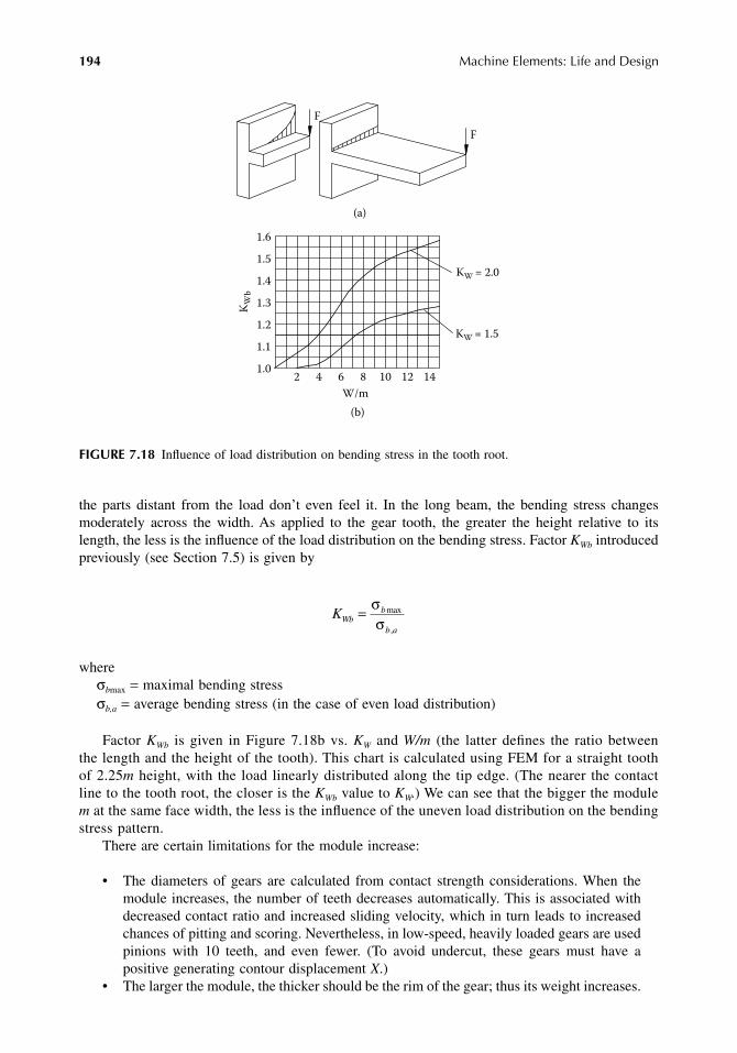
194 Machine Elements: Life and Design
the parts distant from the load don’t even feel it. In the long beam, the bending stress changesmoderately across the width. As applied to the gear tooth, the greater the height relative to itslength, the less is the influence of the load distribution on the bending stress. Factor KWb introducedpreviously (see Section 7.5) is given by
whereσbmax = maximal bending stressσb,a = average bending stress (in the case of even load distribution)
Factor KWb is given in Figure 7.18b vs. KW and W/m (the latter defines the ratio betweenthe length and the height of the tooth). This chart is calculated using FEM for a straight toothof 2.25m height, with the load linearly distributed along the tip edge. (The nearer the contactline to the tooth root, the closer is the KWb value to KW.) We can see that the bigger the modulem at the same face width, the less is the influence of the uneven load distribution on the bendingstress pattern.
There are certain limitations for the module increase:
• The diameters of gears are calculated from contact strength considerations. When themodule increases, the number of teeth decreases automatically. This is associated withdecreased contact ratio and increased sliding velocity, which in turn leads to increasedchances of pitting and scoring. Nevertheless, in low-speed, heavily loaded gears are usedpinions with 10 teeth, and even fewer. (To avoid undercut, these gears must have apositive generating contour displacement X.)
• The larger the module, the thicker should be the rim of the gear; thus its weight increases.
FIGURE 7.18 Influence of load distribution on bending stress in the tooth root.
1.0
1.1
1.2
1.3
1.4
1.5
1.6
2 4 6 8 10 12 14
KW
b
KW = 2.0
W/m
(a)
(b)
F
F
KW = 1.5
KWbb
b a
= σσ
max
,
9563_C007.fm Page 194 Wednesday, July 25, 2007 4:13 PM

Gears 195
Ratio W/m may be decreased also by decreasing the face width of the gear. In this case, thediameters should be increased to meet the strength requirements. The increase in diameter anddecrease in width enable the pinion shaft to be made more rigid and the teeth misalignment,somewhat less.
7.7 DYNAMIC LOAD IN THE GEAR MESH AND FACTOR Kd
Estimation of load applied to the teeth begins by calculating the nominal force Fn: the nominaltorque is divided by the radius of the base circle. But there are some additional forces that shouldbe taken into account.
It is known that in rotating systems, torsional vibrations are unavoidable. In important appli-cations, a dynamic analysis is usually performed, and if the dynamic torque exceeds 5–10% of thenominal torque, the needed changes in mass and torsional stiffness of certain elements should bemade to reduce the amplitude of the alternating torque.
Apart from what has been stated earlier, the dynamic load in the gear mesh is practicallyindependent of the other members of the mechanism. Two engaged gears make a torsionallyoscillating system of two rotating masses connected by an elastic element (the gear mesh). Thestiffness of this element changes in spur gears when the one-pair and two-pair modes take turns.This cyclic change in the stiffness parameter excites vibrations and may lead to what is calledparametric resonance. The resonance frequency may be calculated; if it is close to the toothengagement frequency, either the moments of inertia of the gears or the number of teeth should bechanged, or the contact ratio should be increased to 2 so as to eliminate the parametric excitation.And finally, there are dynamic loads in the gear mesh caused by errors in the geometry and basepitch of the teeth under load. This is what the factor Kd is intended for.
Early in the 20th century, when large steam turbines were developed, high-speed, large-capacityreduction gears came into demand. The technology of gear manufacturing was not able then toprovide very high accuracy of the teeth, and there were cases of teeth breakage during bench runswithout any load. Nowadays, when the rim speed may exceed 200 m/sec (40,000 ft/min), theindustry is equipped with super-precision gear-cutting and finishing machines that allow manufac-turing to very close tolerances, within 1–3 µm for gears of several meters in diameter. So theproblem of accuracy can be solved now quite satisfactorily. But some moderate dynamic loadremains.
Figure 7.19 shows two cases of impact in spur gearing. In the first case (Figure 7.19a), thebase pitch across teeth A1-B1 is less than that across teeth A2-B2. (In the picture, it is shown asinterference between teeth B2 and B1.) As a result, pair B1-B2 comes into contact with an impact.This case is called edge impact because one of the teeth gets the impact at its tip.
FIGURE 7.19 Tooth impact caused by pitch deviations.
(a) (b)
A2
B1
A1 B2
A2A1 B2
B1
Driven gear
Line of action
Driving gear
9563_C007.fm Page 195 Wednesday, July 25, 2007 4:13 PM

196 Machine Elements: Life and Design
In the other case shown in Figure 7.19b, the base pitch across teeth A1-B1 is bigger than thatacross teeth A2-B2. In the position shown, pair A1-A2 disengages and pair B1-B2 remains, kind ofhanging in the air. Because there is no contact between the teeth (for a moment), the driving gearaccelerates, and the driven gear becomes slower. (The same process was described in Section 7.1with reference to a spur gear with contact ratio less than 1.) Therefore, the teeth come into contactwith a “middle impact.”
The edge impact is more dangerous because the force is applied to the tip of a tooth. It resultsin increased noise and, possibly, pitting, scoring, and teeth breakage. Increasing tooth accuracyis not enough to prevent the edge impact. Because of elastic deformation of the teeth under load(shown dashed in Figure 7.20a), the base pitch decreases on the driving gear (teeth A1-B1) andincreases on the driven gear (teeth A2-B2). It is exactly what leads to the edge impact. To preventit, the involute profile of the teeth should be modified by making the tip thinner (Figure 7.20b).The profile relief begins in the upper point of the one-pair zone (about 0.4m from the tooth tip).It is of involute shape with a larger pressure angle. The maximal depth of the profile modificationsusually equals the elastic deformation of the pair engaged in the end of the one-pair zone (A1-A2,in this case).
Because the addendum of one tooth is in contact with the dedendum of its mate, the profilerelief may be done on the addendum, or on both the addendum and the dedendum (in the lattercase, with lesser deviation from the initial involute).
Perhaps a reader who has followed the process this far might still wonder how to obtain theKd value? After all, for the strength calculation, the number only is needed, not the understandingas to how it was reached? At this point, the authors might start speaking in a roundabout way.“Look … ” (This is the usual beginning, when we don’t know exactly what to say, and we try toinvolve the listener in our process of thinking.) “You know, … ” (Possibly, you don’t know, butnever mind.) The only answer the authors can give in the context of this book is as follows.
Dynamic load is a result of a continuous oscillatory process in the vibrating system of twogears. The dynamic load on a certain pair of teeth depends not only on the geometry of this verypair but also on geometry of the preceding pairs. That is why the exact calculation of the dynamicload should be based on exact knowledge of the real geometry of all teeth. It is rather unreal,particularly, taking into consideration that the teeth geometry changes in operation. This processis also influenced by the oil film between the contacting teeth. Nevertheless, there are someacknowledged methods of gear analysis that include the dynamic load calculation as well. Thesemethods are approximate, but experimentally proved and for that reason quite reliable. And themost comforting thing is that when the gears are manufactured with an appropriate accuracy(conforming to the rim speed) and profile modification, the Kd value lies in the range of 1.15–1.35.
FIGURE 7.20 Pitch change caused by deflection under load.
A2
(a) (b)
A1Fn B2
B1
Driving gear
Drivengear
0.4 m
s
9563_C007.fm Page 196 Wednesday, July 25, 2007 4:13 PM

Gears 197
(Certainly, it is not valid for the resonant mode mentioned in the preceding text.) So the possibleerror in estimation of the Kd value looks quite acceptable as compared to other uncertainties of thegear strength calculations. In important cases, the real bending stress should be measured duringtrials. Sometimes, these measurements are performed periodically in service to control the influenceof the changes in gear geometry and in the alignment of teeth.
7.8 LOAD DISTRIBUTION IN DOUBLE-HELICAL GEARS (FACTOR KWh)
Double-helical (“herringbone”) gears are an example of a mechanism with split power transmission(Figure 7.21). Uniform distribution of the load between two halves of the gear is supposed to beachieved by axial self-alignment of the pinion. In the ideal case, when only the meshing forces areapplied to the pinion, the static equilibrium of the pinion implies the equality of axial forces Fa1
and Fa2. The pinion moves axially until this equality is reached. Because the helix angles on theright and on the left are equal, the load should be distributed equally.
It doesn’t rule out possible unevenness of load distribution across each of the half-gears causedby bending and torsion deformations of the pinion under load.
In fact, there are friction forces in bearings, couplings, and between the teeth that hinder thepinion from axial motion. Inertia of the pinion plays the same part. As a result, there is always acertain difference between forces Fa1 and Fa2 and unevenness in load distribution between therespective halves of the gear.
The ability of the pinion for self-alignment depends on several design factors. First of all, thebearings and couplings must enable the needed axial motion. This may be a radial sliding bearingor cylindrical roller bearing without lips on one of the rings (Figure 7.21b). Bearings with one lipmay be used on the understanding that the rings are somewhat displaced from their nominal position,so as to produce axial play needed for the pinion to take the equilibrium position (Figure 7.21c).
The bearings shown in Figure 7.21d seemingly enable the axial movement of the pinion. Butthe friction between the housing and the outer ring of the bearing is too high, and this results in alarge difference between forces Fa1 and Fa2. In the extreme case, at a small helix angle, even thefull-load axial force may be insufficient to move the pinion under load, and then, only one half ofthe gear will transmit the entire load.
FIGURE 7.21 Bearings for double-helical gears.
1
Fa1 Fa2
(a)
(b)
(c)
(d)
Wrong
9563_C007.fm Page 197 Wednesday, July 25, 2007 4:13 PM
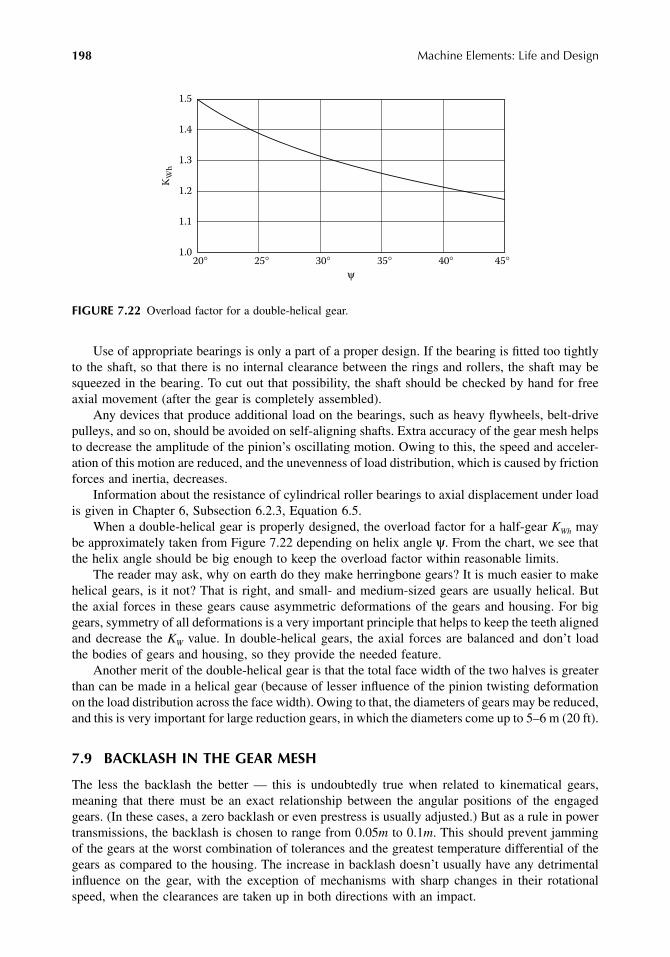
198 Machine Elements: Life and Design
Use of appropriate bearings is only a part of a proper design. If the bearing is fitted too tightlyto the shaft, so that there is no internal clearance between the rings and rollers, the shaft may besqueezed in the bearing. To cut out that possibility, the shaft should be checked by hand for freeaxial movement (after the gear is completely assembled).
Any devices that produce additional load on the bearings, such as heavy flywheels, belt-drivepulleys, and so on, should be avoided on self-aligning shafts. Extra accuracy of the gear mesh helpsto decrease the amplitude of the pinion’s oscillating motion. Owing to this, the speed and acceler-ation of this motion are reduced, and the unevenness of load distribution, which is caused by frictionforces and inertia, decreases.
Information about the resistance of cylindrical roller bearings to axial displacement under loadis given in Chapter 6, Subsection 6.2.3, Equation 6.5.
When a double-helical gear is properly designed, the overload factor for a half-gear KWh maybe approximately taken from Figure 7.22 depending on helix angle ψ. From the chart, we see thatthe helix angle should be big enough to keep the overload factor within reasonable limits.
The reader may ask, why on earth do they make herringbone gears? It is much easier to makehelical gears, is it not? That is right, and small- and medium-sized gears are usually helical. Butthe axial forces in these gears cause asymmetric deformations of the gears and housing. For biggears, symmetry of all deformations is a very important principle that helps to keep the teeth alignedand decrease the KW value. In double-helical gears, the axial forces are balanced and don’t loadthe bodies of gears and housing, so they provide the needed feature.
Another merit of the double-helical gear is that the total face width of the two halves is greaterthan can be made in a helical gear (because of lesser influence of the pinion twisting deformationon the load distribution across the face width). Owing to that, the diameters of gears may be reduced,and this is very important for large reduction gears, in which the diameters come up to 5–6 m (20 ft).
7.9 BACKLASH IN THE GEAR MESH
The less the backlash the better — this is undoubtedly true when related to kinematical gears,meaning that there must be an exact relationship between the angular positions of the engagedgears. (In these cases, a zero backlash or even prestress is usually adjusted.) But as a rule in powertransmissions, the backlash is chosen to range from 0.05m to 0.1m. This should prevent jammingof the gears at the worst combination of tolerances and the greatest temperature differential of thegears as compared to the housing. The increase in backlash doesn’t usually have any detrimentalinfluence on the gear, with the exception of mechanisms with sharp changes in their rotationalspeed, when the clearances are taken up in both directions with an impact.
FIGURE 7.22 Overload factor for a double-helical gear.
KW
h
1.0
1.1
1.2
1.3
1.4
1.5
20° 25° 30° 35° 40° 45°ψ
9563_C007.fm Page 198 Wednesday, July 25, 2007 4:13 PM

Gears 199
In spur gears that work in plenty of oil, and in gear pumps, problems may develop because ofthe displacement of oil from the tooth space by the mating tooth. Figure 7.23a shows the situationin which tooth A enters the tooth space B; at point C, it is in contact with the mating tooth, andthe oil can flow out of the volume B through the opening D (and from the ends, of course). Theoil pressure developed in volume B may be so high that the bearings may be damaged. Increasingthe backlash (say, to 0.1m) will increase the opening D and may sufficiently reduce the oil pressurein this volume and will also reduce power required to drive the pump.
Figure 7.23b shows the beginning of the two-pair zone. The teeth are in contact at points Cand E. At point D, there is a backlash that joins together volumes B and F. As the gears rotate, thisclosed volume (B + F) contracts, and the oil can flow out of it only through the ends. The endsmust be open, and the covers of the pump housing must be provided with grooves that connect theoutlet from volumes B and F with the pumping chamber. But if the pump gears are long, it is notenough, and very high pressure may develop in volumes B and F, which may damage the bearingsor cause shaft breakage. Recesses G in the teeth shown in Figure 7.23c and Figure 7.23d reducethe pressure in the tooth spaces.
Certainly, such recesses can’t be used in power transmissions because they decrease the activeface width and reduce the contact and bending strength of the teeth. But the quantity of oil intransmissions is much less, and the problem of oil pressure may come into being only at highspeed. In these gears, the oil is sprayed onto the teeth after they leave the contact zone or fairlybefore it, so that when they come to contact again, they are covered with a thin oil film only. Thetooth spaces before entering the contact zone are filled with compressible air and oil mist.
In helical gears, tooth contact begins on one end and moves to another, so the oil is freelydisplaced in the direction of the moving contact. In a double-helical gear, the oil may be displacedfrom the center to the sides or from the sides to the center, depending on the direction of teeth and
FIGURE 7.23 Oil drain from the tooth spaces.
B
G
(a)
F
B
C
D
E
C
D
(b)
(d)(c)
A
A
G
Driving
gear Driving gear
Driven gearDriven gear
9563_C007.fm Page 199 Wednesday, July 25, 2007 4:13 PM

200 Machine Elements: Life and Design
direction of rotation. When the oil is displaced to the center, it may cause an additional heating ofthe gears in the middle, increase in their diameters, and uneven load distribution across the facewidth.
7.10 LUBRICATION OF GEARS
The system of lubrication is intended to provide the rubbing surfaces with an oil film and takeaway the heat. The kind of lubricant and type of gear lubrication depend in the first place on thepitch line velocity of a gear. Low-speed gears, particularly those that are open (that means, theydon’t have a hermetically sealed housing), are often greased. The grease is applied to the teeth bybrush once a day or once a week depending on the need. Because the grease is not able to takeoff the heat from the teeth, this type of lubrication is used only for light-duty applications, wherethe small amount of heat may be successfully taken off by convective heat transfer. The recom-mended speed limit for the grease-lubricated open gears is up to 4 m/sec. At a higher speed orcontinuous duty, the periodic manual greasing becomes too laborious and is replaced by dippingone of the gears into an oil-filled pan.
Gears which have a hermetically sealed housing are usually lubricated with oil. As comparedwith grease, oil is more heat resistant, lasting, and easily replaceable. It washes away the weardebris from the wearing surfaces and, by permanent filtering of the oil, the mechanism can be keptclean during long-term usage.
It is particularly important for bearings to be lubricated with clean oil. But the other wearingparts also have sufficiently lesser wear rate when the wear debris is permanently removed from thefriction surfaces. Oil transfers the heat from the teeth to the housing walls, which can be provided,if needed, with fins and fans for more effective cooling.
The simplest way to use liquid oil is by oil bath lubrication (Figure 7.24). To diminish hydrauliclosses, the gears should not be immersed too deeply, but not less than the teeth height. In bevelgears, it is also recommended that the teeth should be entirely immersed in oil.
The oil level should be checked while the gear is running because the oil splashed on the wallsof the housing flows down slowly, and the oil level may become considerably lower than it was inthe nonoperated gear. The authors have observed recession of oil level in a reduction gear by asmuch as 25 mm.
If the oil gauge is placed far from the oil-immersed gear wheel, even a small inclination of thegear housing may result in lack of lubrication. Therefore, the gear should be mounted level on itsfoundation, and the housing should be provided with special horizontal surfaces for mounting thelevel.
To guarantee reliable bath lubrication in a multistage gear set, one gear of each stage shoulddip into the oil. For this purpose, in low-speed gears the oil level can be increased as shown inFigure 7.24a. At higher speed, the smaller gear wheel can be lubricated with an additional idlergear 1 (Figure 7.24b) made of gray cast iron or some kind of plastic. It rotates freely on an axleand supplies oil to the power train. The face width of the idler should be equal to 0.7–0.8 that ofthe lubricated gear. If the width of the idler is relatively small, the load concentrates in the lubricated
FIGURE 7.24 Oil bath lubrication of gears.
(a) (b) (c)
1
9563_C007.fm Page 200 Wednesday, July 25, 2007 4:13 PM

Gears 201
area, because this part of a tooth “protrudes” because of thicker oil film. This may result in severepitting in the area of flooded lubrication. Sometimes the gear is designed with an inclined casingjoint that provides equal dipping for the gears of all stages (Figure 7.24c).
Rolling bearings are usually splash oil fed. It is believed that at oil viscosity less than 250 cSt,reliable splash-oil-feed is achievable when the centrifugal force of the oil drops is greater than theirweight. That means
whereV = linear speed of the mesh (m/sec)R = radius of the gear (m)g = 9.81 m/sec2 = acceleration of gravity
EXAMPLE 7.7
When R = 0.2 m, the linear speed, for satisfactory oil sprinkling, should be not less than
If the oil is sprinkled on the walls of the housing, it doesn’t mean that it gets into the bearings.Investigation of splash oil feed for bearings has been performed on a two-stage reduction gear witha transparent housing made of acrylic plastic. The scheme of this gear and the results of theinvestigation are given in Table 7.1. No special grooves were made to lead the oil to the bearings,but they were completely open and accessible for the air and oil splashes from within. Before eachexperiment, all the bearings were dismounted from the shafts and degreased. Then the gear wasassembled and filled up with oil of needed viscosity, so that the intermediate gear wheel wasimmersed into the oil as deep as two heights of the teeth (as shown in Figure 7.24a). Then the gearwas rotated for 5 min with a certain rotational speed in a certain direction. After that, the gear wasdismantled, the bearings dismounted from the shafts, and the presence of oil on the races androlling elements of the bearings was checked by white filter paper. We have seen that inside thegear there is an oil storm, particularly at higher speeds. It was impossible to imagine that insidethe housing there can be any dry places. But there were, and, in fact, the dry locations were theraces and rolling elements of the bearings!
In Table 7.1, the hatched cases are those in which the bearings were oiled. In the nonhatchedcases, the bearings remained dry. The experiments have shown that without appropriate facilities,splash lubrication of the bearings can’t be guaranteed. There were cases in which (at a highspeed) the oil streamed abundantly down the walls, but tore off the edge of the bearing seat anddidn’t enter the bearing. When the gear was stopped, the oil flow was getting less intensive, andsome small amount of oil was entering the bearing. But such lubrication can’t be considered assatisfactory.
Reliable oil supply to the bearings is achieved by oil-catching grooves 1 (Figure 7.25) madeon the joint surfaces of the housing. In middle-sized gears the grooves are 5–10 mm in depth and10–20 mm in width. The grooves catch the oil that flows down the walls. Dripping-pans serve thesame purpose (Figure 7.26); they collect the splashed oil and lead it to the bearings.
mV
Rm g V gR
2
≥ ≥;
V m s
nVD
rp
= ⋅ =
= = ⋅⋅ ⋅
=
9 81 0 2 1 4
60 60 1 42 0 2
67
. . . /
..π π
mm
9563_C007.fm Page 201 Wednesday, July 25, 2007 4:13 PM

202 Machine Elements: Life and Design
TAB
LE 7
.1B
eari
ng L
ubri
cati
on
25
01
60
42
6
35
BA
1
Dir
ecti
on
of
inp
ut
shaf
tro
tati
on
Oil
vis
cosi
ty, c
St
Ge a
r ra
tio
Nu
mb
er o
f b
eari
ng
15
00
10
00
75
05
00
30
01
50
15
00
10
00
75
05
00
30
01
50
Input shaft speed, rpm
BA
14
12
.7
12
34
56
12
34
56
12
34
56
12
34
56
12
34
56
12
34
56
38
.9
15
0
12
.73
8.9
15
00
12
.73
8.9
9563_C007.fm Page 202 Wednesday, July 25, 2007 4:13 PM

Gears 203
If the gear runs slowly and the sprinkling is insufficient, the oil can be taken off the gear faceby a scraper (2 in Figure 7.25). The tip of the scraper can be installed at a distance of 0.5–1 mmfrom the gear face. If the tip is made of rubber or plastic, it may touch the gear. The scraper shownin Figure 7.25 is designed so that it can take oil off the gear face and lead it to the oil grooveindependent of the gear’s rotational direction.
The oil grooves and ducts are configured so that the oil can flow to the oil reservoir only throughthe bearings. Therefore, bearing lubrication is assured. Gears designed to operate at a wide rangeof working conditions (such as rotational speed, direction of rotation, load, temperature, etc.) shouldhave a lubrication system that assures the proper functioning at any specified conditions. For smallgears, it may be increasing the oil level until all the gear wheels and bearings are partly or completelyimmersed. In these cases, the seals should be of good quality and reliability. For larger gears, aforce-feed lubrication system (with an oil pump) is usually used.
The capacity of the oil reservoir should be big enough to minimize the rate of oil decompositionand give the wear debris a place to settle. Depending on the power transmitted, the volume of oil
FIGURE 7.25 Lubrication grooves and scraper.
FIGURE 7.26 Oil collector and lubrication holes.
Gear face1
1 12
2
Section B-BSection A-A
Lower part
of housing
Upper part
of housing
A
A
B
B
(a) (b)
9563_C007.fm Page 203 Wednesday, July 25, 2007 4:13 PM

204 Machine Elements: Life and Design
is recommended in the range of 3.5–10 l/kw of lost power. For instance, if a two-stage gear transmitspower of 100 kW, and its efficiency is 97%, the recommended oil content is 0.03 · 100(3.5 to 10)= 10.5–30 l. In practice, it is not always achievable, particularly in lightweight machines, such asvehicles, planes, and the like, where the entire mechanism is rather small, and there is no placeavailable for this volume of oil. In these cases, field experience is the best adviser.
The oil level is usually monitored using a dip stick. Figure 7.27a shows a design of dip stickthat allows measuring the oil level while the gear is running. Pipe 1 protects the stick from the oilsplashes. Take note of hole 2 in the upper part of the pipe; the rubber knob of the stick serves alsoas a plug, and if there is no hole in pipe 1, the knob will force the oil out of the pipe and makethe stick indication false.
Widely used level indicators with a transparent face (“sight glasses”) from glass or acrylicplastic are shown in Figure 7.27b. (Some designs use glass tubes rather than flat glass plates.)It is preferable to place the level indicators and dip sticks closer to the gear that is less immersedin oil.
The circulation lubrication system is unavoidable if design or service conditions don’t allowsatisfactory lubrication by immersion and sprinkling; for example, when the gear shafts are vertical,or when the speed is too high or too slow, or when the lubrication system contains oil filters, heatexchanger, and other devices that need forced circulation. Sliding bearings, usually, also need force-feed lubrication.
Oil circulation is commonly provided by a gear-type pump or plunger pump, attached to thegear housing and driven by one of the gear shafts. The gear-type pump is preferable in a reversibleversion (with appropriate valving) so that the lubrication system and the gear will not be damagedif the gear is accidentally reversed.
In middle-sized gears, the pump usually takes the oil from the gear housing and supplies itthrough oil ducts to the gear mesh and the bearings. The capacity of the oil reservoir is usuallychosen as large as the pump can supply in 0.5–2 min, depending on the design features.
In bigger gears, which transmit great power, the lubrication system may include, besides theassociated pump, the following:
• An electric pump for oil circulation before setting the machine in operation• An oil tank with a capacity that equals the pump supply during 3–4 min or more
FIGURE 7.27 Oil level indicators.
A
A
Section A-A
(a) (b)
1
2
9563_C007.fm Page 204 Wednesday, July 25, 2007 4:13 PM

Gears 205
• An oil cooler and, possibly, also a heater (to heat the oil before starting, lest the oilpressure in the system be too high in the beginning because of increased flow resistance)
• Oil filters• Indicator of metal particles in the oil• Safety valves• Manometers, thermometers, and alarm devices that alert the personnel when the pressure
and the temperature of the oil deviate from the permissible values, and other devices
The recommended quantity of oil to be sprinkled on the gear teeth is about 5–8 l/min perkilowatt of power wasted in the mesh (about 1.5% of the power transmitted). At this quantity, theoil warms up by 8–5°C, correspondingly.
With force-feed lubrication, uniform distribution of oil across the face width of the gears isachieved using pipelike sprayers with several holes (Figure 7.28a). To avoid their clogging, thediameter of these holes should not be less than 0.8 mm (usually, 1.2–3.0 mm). The oil flow throughone hole depends on its diameter, oil pressure, and oil viscosity. At the viscosity of 110 cSt, theoil flow is approximately
whered = diameter of the hole (mm)p = oil pressure (MPa)
For example: d = 2 mm, p = 0.3 MPa, Q = 3.5 l/min.Narrow gears may be lubricated by a sprayer as shown in Figure 7.28b and Figure 7.28c.
Dimensions of the jet and oil flow for the option as shown in Figure 7.28c are given in the chartsand table.9
FIGURE 7.28 Oil sprayers.
Q d p l= 1 6 2. /min
(a)
(d)
(c)
(b)
H
L
040
40
80
120
160
200
80 120 160
H (mm)
1
2
3
4
Curve No Oil flow
l/min
12
43
Oil pressure
MPa
0.0500.025
0.0750.100
1.21.72.22.6
∅14
0.8
5∅11
L (
mm
)
9563_C007.fm Page 205 Wednesday, July 25, 2007 4:13 PM

206 Machine Elements: Life and Design
In high-speed gears, there may occur erosion of metal in places where the teeth hit the oil jet.In these cases, a sprayer as shown in Figure 7.28d may be useful. It fragments the oil jet and createssome mixture of air and small particles of oil.
The most effective cooling of teeth is achieved when the oil is directed at the beginning ofthe teeth engagement, as shown in Figure 7.29a. This method is recommended up to a speed of20 m/sec for spur gears and up to 50 m/sec for helical gears. For high-speed gears, particularlyspur gears, this method is unsuitable, because when the oil is forced out of the tooth spaces ina very short time, there may be created a very high hydrodynamic oil pressure. This pressureoccurs cyclically with the teeth engagement frequency and may lead to severe vibrations andfailure of gear elements (bearings, shafts, housing, etc.). In these cases, the oil should be sprinkledas shown in Figure 7.29b. If the oil picks up insufficient heat, additional sprayers can be installed(Figure 7.29c).
The sprayers and all elements of the piping should be rigid and strong lest they be broken fromvibrations. The natural frequencies of the elements of lubrication system should not be close to theteeth engagement frequency. It is desirable to locate the bolt connections so that an undone nut, apiece of a broken cotter pin, or lock wire can’t fall and get into the gear mesh. Among the suitablelocking element types, tab washers and locking plates are the best.
When the prototype gear is assembled, the lubrication system should be pumped with oil tocheck whether the jets get exactly to the needed places. This is particularly important when thesprayers are distant from the lubricated surfaces. If the rotational speed of the gear changes in thecourse of operation, the pump delivery changes as well. In this case, the pump should be designedfor excessive oil supply at high speed and provided with an overflow valve to keep constant oilpressure in the system. In addition, the shape, position, and range of the oil jets must be designedto deliver adequate lubrication at all pressures and speeds.
Example of force-feed lubrication for a reduction gear with vertical shafts is shown inFigure 7.30. Pump plunger 1 is set in motion by cam 2 mounted on the end of the intermediateshaft of the gear. The oil comes through ducts 3 and 4 into the upper housing, and there it isdistributed among the bearings and gears. The low-speed stage is lubricated by sprayer 5. Asmall part of the oil flows through oil indicator 6, so that the oil flow can be seen inside aglass pipe.
Figure 7.31 shows a two-stage reduction gear with a bevel input stage and planetary outputstage. The gear is lubricated by a gear-type pump 1, which sucks the oil from the lower housingthrough inlet pipe 2 and forces it into outlet pipe 3. From there the oil flows through a filter to thebearings and gears. Bearing 4 is greased through pipe 5. Labyrinth seal 6 protects the bearingchamber from ingress of dirt and retains the grease. Rotating collar 7 prevents the entrance of liquidoil into that chamber.
FIGURE 7.29 Direction of oil spray on gears.
(b) (c)(a)
αα/2
9563_C007.fm Page 206 Wednesday, July 25, 2007 4:13 PM

Gears 207
FIGURE 7.30 Three-stage reduction gear with vertical shafts.
FIGURE 7.31 Two-stage bevel-planetary gear with vertical output shaft.
7
8
1 2
5
4 6
3
Oil level
9
9 8
10
5
4
6
21
3
7
Oil level
9563_C007.fm Page 207 Wednesday, July 25, 2007 4:13 PM

208 Machine Elements: Life and Design
7.11 COOLING OF GEARS
Almost the entire power wasted in mechanisms turns into heat. The efficiency of gears dependson their kind. Ordinary spur, helical, and bevel gears are quite efficient. From 1.5% to 3% of thepower transmitted is spent in one gear stage partly on friction in the mesh and bearings, andthe rest on oil agitation (called hydraulic loss). Planetary gears have the same or higherefficiency. In small gears of this kind, the cooling problem usually doesn’t exist, because theconvective heat exchange satisfies the requirements. But the power transmitted by a gear isnearly proportional to the third power of its dimension, whereas the area of the heat-exchangesurfaces is proportional to the second power only. So in larger gears that transmit several tensof kilowatts and more, cooling may present difficulties and needs thorough calculation andorganization.
In gears with a high ratio in one stage (such as worm gears, harmonic drives, and some specialkinds of planetary gears called fixed differentials10), the power loss may be as great as 50% andmore at a ratio of 1:80. Though these gears usually transmit relatively small power, their coolingmay present difficulties and restrict the allowable working load at a constant duty. So, coolingproblems can be dealt with in small gears as well as in the big ones.
The calculation of cooling begins with the determination of heat input. The efficiency η of agear is mostly taken relying on recommendations; otherwise, it should be determined experimen-tally. Virtually all the power loss turns into heat, so the heat input Pin is given by
(7.23)
Here P = power on the input shaft of a gear (kW).The output energy Pout (that is, the heat removal from the gear) depends on the area A (m2) of
the heat-exchange surfaces, the temperature difference ∆t (°C) between the gear (tg) and thesurrounding medium (ts), and also on factor k that shows how much energy (W) can be removedfrom 1 m2 of a surface if the temperature difference ∆t = 1°C:
(7.24)
Factor k is called the heat transfer factor and is dimensioned in W/(m2 · °C). It has a perfectlyclear physical meaning, but very vague numerical value that depends on the material of thegear housing, on how it is painted if at all, on how it is cleaned from dust and oil, on the kindof surrounding fluid medium and its speed relative to the heat-exchange surface, and others.The rotational speed of the shafts affects the heat exchange very much: the higher the speed,the more intensive and uniform the heat transfer is from the oil to the housing walls and thegreater the fanning effect of the rotating couplings. The practical recommendations are asfollows:11
• For housings without fan cooling,
k = 10–25 W/(m2 · °C)
• The smaller values are recommended for painted housings of steel and gray iron, lowrotational speed, and dusty air; the greater values, for aluminum nonpainted housings,rotational speed of 1500 r/min and more, and clear air.
• Bottom surfaces of the housing are less efficient in convection, but part of the heat energyis transferred in that area through metallic contact of the mount feet into the frame or
P P Win = −( )1 103η
P A t t k A t k Wout g s= − = ⋅ ⋅( ) ∆
9563_C007.fm Page 208 Wednesday, July 25, 2007 4:13 PM

Gears 209
base the housing is attached to. Therefore, with regard to inaccuracy of all this calculation,the bottom surface can be calculated together with the other walls, if there is enoughspace for the air to pass under it.
• Ribs made to increase the heat-exchange surface are less effective than the wall becausetheir temperature gradually decreases with distance from the wall. Therefore, it is rec-ommended to take into account 50% of their surface (say, only one side of a rib).
• For blower cooling,
where v = air speed (m/sec).• For example, if v = 10 m/sec, k = 45 W/(m2 · °C). As one can see, fanning is a very
effective means to intensify the cooling process.
Further reduction of the oil temperature can be achieved by insertion of a water pipe into theoil reservoir. The value of factor k for the water pipe depends on the circumferential speed of theoil-dipped gear wheel and the speed of the water in the pipe. For copper alloy tubes, it ranges fromabout 150 W/(m2 · °C) for a gear speed of 4 m/sec and a water flow speed of 0.1 m/sec to about200 W/(m2 · °C) for a gear speed of 12 m/sec and a water speed of 0.4 m/sec. Steel tubes providea factor k smaller by 5–10%.
As shown, the participants in the heat extraction process may have different capabilities. Foreach of them the Pout amount should be calculated separately using Equation 7.24 and thensummarized:
(7.25)
Before the gear is set in motion, its temperature equals mostly that of the surroundings: tg
= ts (unless it had been previously warmed up or chilled). When the gear begins to work, itimmediately begins receiving the Pin amount of heat energy and starts warming up. As thetemperature increases, the Pout value rises in direct proportion to the temperature difference, butthe rate of temperature increase gradually approaches zero (Figure 7.32a) as Pout approachesPin. From this moment on, the gear doesn’t change its temperature, because the input and outputamounts of heat have become equal:
FIGURE 7.32 Process of heating and cooling.
k v W m C= + ⋅ °7 12 2/( )
P P A t kout out i i i i= = ⋅ ⋅Σ Σ ∆, ( )
P Pin out=
(a) (b)
Time
Tem
per
atu
re
9563_C007.fm Page 209 Wednesday, July 25, 2007 4:13 PM
210 Machine Elements: Life and Design
Equating of Equation 7.23 and Equation 7.25 gives directly the steady-state temperature difference between the gear and the surroundings for the case when ∆t is nearly the same for all the participants of the heat extraction process:
If ∆t differs (for example, the air temperature is 30°C, and the water in the pipe is 15°C), calculationof ∆t value can be done by iterations.
As soon as the ∆t value has been determined, we can know the gear temperature: tg = ts + ∆t.The gear temperature should not exceed the value permissible for the oil, which equals approxi-mately 70°C (rarely 80–90°C). If the cooling calculation shows that the gear temperature is higherthan admissible, appropriate measures must be taken to ensure an acceptable level of cooling.Besides those mentioned previously, an additional heat exchanger of needed capacity with oilcirculation system can be used. For large gears that transmit hundreds and thousands of kilowatts,this is the only means to keep the oil temperature within admissible limits.
In fact, tg is the temperature of the outer surface of the housing. The temperature of the oil isa bit higher. The gear wheel dipped into the oil has nearly the same temperature, but the pinion isusually distinctly warmer. What is mainly of interest to us is the oil temperature, because the oil,if overheated, is not able to form a protective layer on the metal surface (see Chapter 6,Subsection 6.3.1). It should be kept in mind that the oil undergoes an additional heating in the gearmesh, so the recommended temperature of the oil should not be exceeded.
The preceding formulas are valid for constant duty. When the load is changing cyclically, thePin value in Equation 7.23 can be determined as follows:
wherePin,i = power loss in the cycle while transmitting power Pi
ti = time of transmission of power Pi within one cycletc = cycle time
The less the load, the less is the efficiency of the gear. The difference can be significant, andit should be taken into consideration when calculating the Pin,i values using Equation 7.23.
For intermittent duty, when the idle time is long enough to get the gear cooled off, the temperaturecurves at warming up and chilling as shown in Figure 7.32a and Figure 7.32b. For this process, thecalculation should take into account that part of the energy loss is spent to warm up the elements ofthe gear and the rest is dissipated into the surroundings. The temperature of the gear at the end of thework cycle (when ∆t is nearly the same for all the participants of the heat extraction process) can beobtained from the following formula;6
(7.26)
where
∆Σ
tP
A ki i
= −⋅
( )1 103η
PP t
tinin i i
c
=Σ , ,
t tN
A k eg si i
= + − −
( )1 101
13ηαΣ
α =+
t A k
m c m cc i i
m m o o
Σ
9563_C007.fm Page 210 Wednesday, July 25, 2007 4:13 PM

Gears 211
mm = mass of metallic parts of the gear (kg)mo = mass of oil (kg)cm ≈ 0.13 W · h/(kg · °C), specific heat of metallic partsco ≈ 0.56 W · h/(kg · °C), specific heat of oil
EXAMPLE 7.8
The reduction gear shown in Figure 7.25 transmits a continuous load of 30 kW. The efficiency ofthe gear η = 0.96. The gear is indoors, protected from solar heating, and the temperature of the airin summer ts = 30°C. What can be the oil temperature without any additional cooling means?
From Equation 7.23, the input heat energy is
The outer area of the housing A = 0.8 m2. Taking k = 18 W/(m2 · °C), we determine the output energy:
Equating Pin and Pout, we obtain the temperature difference between the housing and the air:
Because the air temperature ts = 30°C, the housing temperature tg = ts + ∆t = 113.3°C. Such ahigh temperature is unacceptable, and the gear must be provided with some additional coolingdevices. Let’s try to apply blower cooling to one side and the top walls of the gear. At an air speedof 10 m/sec, k = 45 W/m2 · °C. The fanned area is 0.3 m2, and the rest is 0.5 m2. Therefore, theoutput energy is given by
We can see that blowing is helpful, but the temperature is still too high, we don’t want it toexceed 70°C. Let’s cancel the blowing and build a water pipe into the oil reservoir. A pipe of30 mm in diameter bent in U form measures about 1 m in length. The area of its outer surfaceequals 0.094 m2. The average value of k = 170 W/m2 · °C. The water temperature is 20°C. So, forthe water pipe the temperature difference tw = 70 – 20 = 50°C, while for the outer surface of thehousing that contacts with the air ta = 70 – 30 = 40°C. Now let’s calculate the output energy at thedesired 70°C of the oil:
That amount is greater than the input energy (Nin = 1200 W), so the real temperature of the oilis believed to be less than 70°C. We can see that the water pipe is very effective.
P Win = − =30 1 0 96 10 12003( . )
P t t Wout = ⋅ ⋅ = ⋅0 8 18 14 4. .∆ ∆
∆t C= = °120014 4
83 3.
.
N t t W
t
out = ⋅ + ⋅ = ⋅
= =
( . . ) .
.
0 5 18 0 3 45 22 5
120022 5
∆ ∆
∆ 553 3
30 53 3 83 3
.
. .
°
= + = °
C
t Cg
N Wout = ⋅ ⋅ + ⋅ ⋅ =0 094 170 50 0 8 18 40 1375. .
9563_C007.fm Page 211 Wednesday, July 25, 2007 4:13 PM

212 Machine Elements: Life and Design
Let’s calculate now how much time that gear with no additional cooling devices can transmitpower of 30 kW until the oil temperature reaches 70°C. The weight of the gear is about 100 kg,and the weight of oil is 4.5 kg. For this purpose we can use Equation 7.26:
That means that the gear may work 42 min before it warms up to 70°C. Do you believe inthat? We don’t! Well, we will check that result using the simplified approach and different unitsof energy. As we know from school, 1 W · h = 0.86 kcal. From here the specific heat of the metalcm ≈ 0.11 kcal/(kg · °C), and that of the oil co ≈ 0.48 kcal/(kg · °C). The amount of heat neededto warm up 4.5 kg of oil and 100 kg of metal by 40°C (from 30°C to 70°C) is given by
The heat energy supplied for this purpose Qsup is given by
The former calculation using Equation 7.26 had shown that the Qneeded is supplied during 0.705 h.Let’s check this result. The input energy during this time we know exactly (provided that theefficiency of the gear we know for certain):
We can’t calculate the output energy exactly because the temperature is changing during this hour.The temperature difference ∆t changes from zero to 40°C. Let’s calculate approximately the Qout
assuming that the temperature difference doesn’t change and equals its average value: ∆t = 20°C. FromEquation 7.24 (with changed units) and taking into account that factor k = 18 W/(m2 · °C) = 15.5kcal/(m2 · h · °C), the output energy during this time is
From here, the supplied heat energy is given by
This result differs only 5% from 526 kcal, so the calculation using Equation 7.26 was correct.
te
Cg = + −⋅
−
= °3030 1 0 96 10
0 8 181
170
1
3( . ).
;α
−−
= = =
= ⋅
10 48 1 923 0 6539
0 8
ee
tc
αα α
α
. ; . ; . ;
. ⋅⋅⋅ + ⋅
=
= ⋅
184 5 0 56 100 0 13
0 6539
0 6539 4 5
. . .. ;
. ( .tc
⋅⋅ + ⋅⋅
=0 56 100 0 130 8 18
0 705. . )
.. h
Q kcalneeded = ⋅ + ⋅ =( . . . )0 48 4 5 0 11 100 40 526
Q Q Qin outsup = −
Q Nin = ⋅ − = ⋅ − =860 1 0 705 860 30 1 0 96 0 705 728( ) . ( . ) .η kkcal
Q kcalout = ⋅ ⋅ ⋅ =0 8 15 5 20 0 705 175. . .
Q kcalsup = − =728 175 553
9563_C007.fm Page 212 Wednesday, July 25, 2007 4:13 PM

Gears 213
REFERENCES
1. Klebanov, B.M., Contact Strength of Spur Gears, in collection of articles entitled, Toothed and WormGears, Kolchin, N.I., Ed., Mashinostroenie, Leningrad, 1974 (in Russian).
2. Reduction Gears of Power Plants Handbook, Derzhavets, Y.A., Ed., Mashinostroenie, Leningrad, 1985(in Russian).
3. Niemann, G., Maschinenelemente, Bd. II., Springer-Verlag, Berlin, Heidelberg, New York, 1965 (inGerman).
4. Kudriavtsev, V.N., Kuzmin, I.S., and Philipenkov, A.L., Calculation and design of gears, Politechnika,Sanct-Petersburg, 1993 (in Russian).
5. Planetary Gears Handbook, Kudriavtsev, V.N. and Kirdiashev, V.N., Eds., Mashinostroenie, Lenin-grad, 1977 (in Russian).
6. Kudriavtsev, V.N., Machine Elements, Mashinostroenie, Leningrad, 1980 (in Russian).7. Kudriavtsev, V.N., Simplified Calculations of Gears, Mashinostrienie, Leningrad, 1967 (in Russian).8. Klebanov, B.M., About the permissible unevenness of load distribution across the face width of a
gear, Transactions of the Leningrad Mechanical Institute, No. 61, Leningrad, 1967 (in Russian).9. Mazirin, I.V., Lubrication devices of machines, Mashgiz, Moscow, 1963 (in Russian).
10. Dudley, D.W., Gear Handbook, McGraw-Hill, New York, Toronto, London, Sydney, 1962.11. Levitan, Y.V., Obmornov, V.P., and Vasiliev, V.I., Worm Gears Handbook, Mashinostroenie, Leningrad,
1985 (in Russian).
9563_C007.fm Page 213 Wednesday, July 25, 2007 4:13 PM

9563_C007.fm Page 214 Wednesday, July 25, 2007 4:13 PM

215
8
Gear Design
All gears have one common element: their teeth. In all other respects, the shapes and structures ofgears may differ very much. Figure 8.1 shows several typical shapes of gears: pinion shafts(Figure 8.1a and Figure 8.1b), gears mounted on shafts (Figure 8.1c to Figure 8.1f), sun wheelsof planetary gears (Figure 8.1g and Figure 8.1h), planet wheels (Figure 8.1i and Figure 8.1j), andring gears (Figure 8.1k and Figure 8.1l). In this chapter, we will mainly discuss simple gearings.
8.1 GEAR AND SHAFT: INTEGRATE OR SEPARATE?
When the gear must be rigidly connected to the shaft, the designer is often unsure about what ispreferable: to make the gear as an integral part of the shaft or to make it apart and connect it tothe shaft by some means. Sometimes, the split design is impracticable because the diameters ofthe shaft and the pinion are very similar (Figure 8.2a).
The diameter of the pinion can even be less than that of the shaft (Figure 8.2b). It may beassociated with the need to increase the bending rigidity of the shaft or with unification of itsbearings (when gears with different ratios are produced in the same housing).
Sometimes the split design is dictated by assembly needs or by manufacturing limitations(for example, when the shaft is too long to be installed on an available gear-cutting machine).Perhaps, the gear teeth must be case-hardened but this can’t be done along with the shaft on theexisting equipment or it requires some additional equipment to decrease the warpage of the shaft.When there are no such constraining conditions, economic considerations prevail in makingdesign decisions.
Yet the split design may result in increased weight, lesser accuracy because of tolerancesummation (also called
stack-up
) and decreased reliability. Figure 8.3 shows some design optionsfor forged gears: those made together with the shaft (Figure 8.3a) and separate from the shaft(Figure 8.3b and Figure 8.3c). Figure 8.4 shows the same for welded gears. Not only is thedismountable connection between the gear and the shaft expensive, but it may also cause problemsin service. Wear, fretting, or both may occur on the splines and centering surfaces, and the nutsmay lose tension or even break completely. This, in turn, may lead to damage or breakage of thegear teeth.
Shaft areas damaged by fretting, as well as stress concentration areas near the splines andkeyways and in the interference fits, provide the best conditions for origination of fatigue cracksthat may lead to shaft failure. This caution doesn’t mean that connections of all kinds should becompletely avoided. But, when making a decision about gear-and-shaft design, reliability shouldcarry weight along with other factors.
One might say that modern methods of calculation enable the design of completely reliableconnections, so that a factor of reliability (or
safety factor
) need not be used. The authors are notready to agree with this opinion. Although our knowledge in the field of machine design hasincreased, troubles during development of machines, as well as in service, have not declined. Thepoint is that the intensity of machines grows relentlessly, and the demand for higher power density(reduced weight and increased capacity) grows hourly. New steels that have doubled and tripledtensile strength are extensively used, but the elasticity modulus of these steels remains the same.Therefore, the higher stresses are accompanied by greater elastic deformations, which, in turn,lead to increased micromovements in connections and hence to damage of the mating surfaces
9563_C008.fm Page 215 Wednesday, July 25, 2007 4:21 PM

216
Machine Elements: Life and Design
FIGURE 8.1
Common gear types.
FIGURE 8.2
Design of pinion shafts.
FIGURE 8.3
Connection of a gear to shaft.
(a) (c)
(b) (h)
(g) (i)
(j) (k) (l)
(d)
(e) (f )
(a)
(b)
(a) (b) (c)
9563_C008.fm Page 216 Wednesday, July 25, 2007 4:21 PM

Gear Design
217
(see Chapter 2). In addition, high-strength materials are more sensitive to stress raisers, especiallyto fretting. The complexity of the processes occurring in the connections doesn’t enable us topredict for certain the service life of heavily loaded joints. As a result, we can’t be confident in thereliability of a machine until it is duly tested.
8.2 SPUR AND HELICAL GEARS
The typical disk-type gear (Figure 8.5a) consists of toothed rim 1 and hub 2 linked to each otherby disk 3. Dimensions of these elements are chosen to impart strength and stiffness to the gear.The most important in this regard are thicknesses of the rim (
δ
1
) and the disk (
δ
2
). The thinner therim, the greater is the bending deformation of the teeth, because bending of the rim is added tobending and shear of the tooth itself (see Figure 8.6a). Because the bending compliance of the rimis not uniform across the face width (it is more rigid in the area of the disk), the tooth complianceis also not uniform. This influences the load distribution along the face width: the more rigid partof the tooth is more loaded (Figure 8.7a). The thicker the rim, the more uniform (less uneven) isthe tooth rigidity, but the weight of the gear increases considerably. In usual practice, the rimthickness
δ
1
is approximately equal to the height of the tooth (about 2
m
).
FIGURE 8.4
Gears welded to a shaft or hub.
FIGURE 8.5
Shapes of gears.
d1
1
(a) (b) (d) (e) (f )
1
3
2
δ2
δ1
(c)
W
R
9563_C008.fm Page 217 Wednesday, July 25, 2007 4:21 PM

218
Machine Elements: Life and Design
Bending of the rim not only influences the teeth elastic compliance, but also may be the placeof failure. If the rim is thick enough, the fatigue crack originated in the root of the tooth propagatesas shown in Figure 8.6b. If the rim is thinner than 1.6
m
, the crack may propagate into the rim(Figure 8.6c) and result in a very grave failure. It is more serious than just tooth breakage becauseit leads to immediate failure of the mechanism, and the repair involved may also be more extensive.Therefore, the rim should be made strong enough. When the weight of the gear is critical, the rimcan be provided with ring ribs as shown in Figure 8.5f and Figure 8.7d.
Because of the increased rigidity of the teeth in the disk area, the maximal unit load of thetooth, as shown in Figure 8.7a, may exceed the average value by about 30% at
δ
1
=
2
m
. Moreuniform load distribution is achieved when the pliable parts of a tooth contact with the rigid partsof the mating tooth (Figure 8.7b and Figure 8.7c). The aforementioned ring ribs (Figure 8.7d) servethe same purpose.
Here is one example from practice. In the course of development of a propulsion gear, therewas frequent tooth breakage of a gear designed as shown in Figure 8.7a. After the design waschanged to that shown in Figure 8.7c, these failures ceased.
The disk thickness
δ
2
for spur gears is dictated by its strength. At a static or momentary load,the weak place is the inner diameter of the disk. When the gear rotates, the stress in this placeremains almost unchanged. But on the outer diameter, the disk is exposed (along with the rim) toalternating bending stress (Figure 8.6d), and a fatigue failure may completely separate the rim fromthe disk.
FIGURE 8.6
Bending deformation and failure of toothed rim.
FIGURE 8.7
Load distribution across the gear face.
(b) (c) (d)
(a)0
σ
Fn
(a) (b) (c) (d)
δ1
δ2
9563_C008.fm Page 218 Wednesday, July 25, 2007 4:21 PM
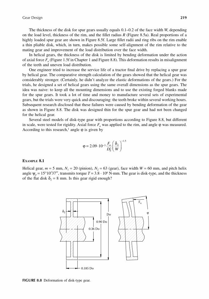
Gear Design
219
The thickness of the disk for spur gears usually equals 0.1–0.2 of the face width
W
, dependingon the load level, thickness of the rim, and the fillet radius
R
(Figure 8.5a). Real proportions of ahighly loaded spur gear are shown in Figure 8.5f. Large fillet radii and ring ribs on the rim enablea thin pliable disk, which, in turn, makes possible some self-alignment of the rim relative to themating gear and improvement of the load distribution over the face width.
In helical gears, the thickness of the disk is limited by bending deformation under the actionof axial force
F
a
(Figure 1.5f in Chapter 1 and Figure 8.8). This deformation results in misalignmentof the teeth and uneven load distribution.
One engineer tried to increase the service life of a tractor final drive by replacing a spur gearby helical gear. The comparative strength calculation of the gears showed that the helical gear wasconsiderably stronger. (Certainly, he didn’t analyze the elastic deformations of the gears.) For thetrials, he designed a set of helical gears using the same overall dimensions as the spur gears. Theidea was naive: to keep all the mounting dimensions and to use the existing forged blanks madefor the spur gears. It took a lot of time and money to manufacture several sets of experimentalgears, but the trials were very quick and discouraging: the teeth broke within several working hours.Subsequent research disclosed that these failures were caused by bending deformation of the gearas shown in Figure 8.8. The disk was designed thin for the spur gear and had not been changedfor the helical gear.
Several steel models of disk-type gear with proportions according to Figure 8.8, but differentin scale, were tested for rigidity. Axial force
F
a
was applied to the rim, and angle
ϕ
was measured.According to this research,
1
angle
ϕ
is given by
E
XAMPLE
8.1
Helical gear,
m
=
5 mm,
N
1
=
20 (pinion),
N
2
=
63 (gear), face width
W
=
60 mm, and pitch helixangle
ψ
p
=
15
°
10
′
37
′′
, transmits torque
T
=
3.8 · 10
6
N·mm. The gear is disk-type, and the thicknessof the flat disk
δ
2
=
8 mm. Is this gear rigid enough?
FIGURE 8.8
Deformation of disk-type gear.
ϕ δ= ⋅
−
−
2 09 10 3
02
2
1 5
..
F
D Wa
δ2
Fa
0.90 Do
0.36 Do
0.185 Do
Doϕ
9563_C008.fm Page 219 Wednesday, July 25, 2007 4:21 PM

220
Machine Elements: Life and Design
Pitch diameter of the gear
Approximate outer diameter of the rim, taking into account Equation 8.3:
The circumferential force
The axial force
The angle of inclination of the toothed rim
Now we can calculate the factor
K
W
(unevenness of load distribution across the face width)using Equation 7.17:
Here,
γ
=
angle of misalignment in the plane of action:
where
α
S
=
pressure angle determined from the formula
C
=
rigidity of the teeth defined by a formula given in Example 7.6:
dm N
mmP = = ⋅′ ′′
=cos cos
.ψ
5 6315 10 37
326 4°
D d m mP0 2 1 25 2 0 22 0 009 326 4 2 5 5 2≈ − ⋅ + + = − ⋅ +. ( . . ) . .ψ ⋅⋅ + ⋅ =5 0 22 0 009 15 177 317 4( . . . ) . mm
FT
dN
P
= = ⋅ ⋅ =2 2 3 8 10326 4
232846.
.
F F Na = = ′ ′′ =tan tanψ 23284 15 10 37 6316°
ϕ = ⋅
= ⋅−
−
−2 09 106316
317 4860
2 69 1032
1 5
..
..
33 rad
KW CqW
a
= 2 γ
γ ϕ α= sin S
tantancos
αψS = °20
110 0 0514
0 1425 0 18603
1 2C N Ne e
= + +
− .
. .
, ,
9563_C008.fm Page 220 Wednesday, July 25, 2007 4:21 PM

Gear Design
221
where
q
a
=
average unit load, which is
From these relations, we have the following:
As we can see, the thickness of the disk should be increased.
Notes: 1. If K
W
< 2, it should be calculated using Equation 7.18.2. This calculation is true if the helical gear proportions are as shown in Figure 8.8. In
other cases, the deformation of the gear should be analyzed by numerical means.
As the disk thickness decreases, the weight of the gear also decreases, but the permissible loaddecreases as well. The minimal weight per unit of transferred torque may be achieved when thedisk thickness is chosen from Figure 8.9a (for gray cast iron housings) or Figure 8.9b (for lighthousings of aluminum or magnesium alloy). These calculations were performed for some averagegear proportions, and their ability to run-in was taken into account. In important cases, special
FIGURE 8.9
Recommended disk thickness of gears.
NN
Ne e113 3 2
2015 10 37
22 2563
, .cos cos. ;= =
′ ′′= =
ψ ° ccos.
315 10 3770 08
° ′ ′′=
qF
WN mma = = =23284
60388 /
tan tan 20
cos15 10 370.377123; 20 3S Sα α= °
° ′ ′′= = ° ′′ ′′
= ⋅ ⋅ ′ ′′ = ⋅− −
9 45
2.69 10 sin 20 39 45 0.95 10 r3 0 3γ aad
1C
10 0.05140.142522.25
0.186070.08
3= + +
−
= ⋅ =
= ⋅ ⋅ ⋅
−
−
6.05 10 ; C 16530 N/mm
K2 0.95 10 6
5 2
W
3 00 16530388
2.2⋅ =
0.1
0.3
0.5ψ = 30°
15°
(b)
200 300 400 500 600
Tooth hardness, HB
δ 2/W 8°
0.1
0.3
0.5
0.7ψ = 30°
15°
(a)
200 300 400 500 600
Tooth hardness, HB
δ 2/W
8°
9563_C008.fm Page 221 Wednesday, July 25, 2007 4:21 PM

222
Machine Elements: Life and Design
analyses of the design should be done. Sometimes gear deformation is useful because it maycompensate for deformations of the shafts and other elements (subject to direction of deformations).
Considerable increase in stiffness of the disk may be achieved by making it conical. In Figure 8.10are given results of experiments
1
with steel models having proportions shown in Figure 8.8. (Conicaldisks are also very useful and widely used in wheels and pulleys in a large variety of applications.)
Holes in the disk should be made minimal in size and number, because large holes cause unevenrigidity around the circumference, as well as less rigidity overall. This unevenness also providesparametric excitation of bending and axial vibrations and may lead at high speed to resonance oscil-lations. In high-speed gears, the possibility of tooth frequency excitation should also be considered.
When the weight of the gear is not restricted (for instance, in stationary equipment), the design ofthe gears is defined by manufacturing and economic considerations. Small and middle-sized gears areforged to reduce machining (Figure 8.5c and Figure 8.5d). Gears with case-hardened teeth are usuallyheat-treated as massive disks (Figure 8.5e) to diminish their warpage. The steel after heat treatment israther hard and intractable, and, if the weight is not strongly restricted, only the exact surfaces of theheat-treated gear (the joint and location surfaces and working surfaces of the teeth) are machined. Ifthe weight must be kept minimal, the excess material is removed by machining (Figure 8.5f).
The gear shown in Figure 8.5f looks beautiful and is an excellent example of the well-knownphrase, “form follows function.” But it is very costly, and were it not for very practical consider-ations, it would not be shaped that way. After all, the gear works inside the housing, and nobodycan enjoy its beautiful shape. This gear is part of a transport machine, and much effort andproduction costs were expended to make it both lightweight and reliable. Its shape, full of gracefulcurves, symmetry, and pleasing proportion, is not due to an artist’s arbitrary whim, but rather isthe result of careful design, stress calculation, and development.
The central part of the gear, called the hub, serves to connect it with the shaft, and its shapedepends on the type of connection. A splined hub may be rather thin-walled; its outer diametermay be set equal to about 1.13–1.25 of the outer diameter of the spline. For an interference-fitconnection, the hub outer diameter usually equals 1.5–1.6 of the shaft diameter (see Figure 8.3c).
At times, the hub includes bearing seats (Figure 8.5f). At other times, a hub is not used, andthe disk of the gear is directly attached to the shaft by bolts (Figure 8.11). The commonly usedproportions in this design are as follows:
FIGURE 8.10
Rigidity of gears with conical gears.
10° 15° 20° 30°
ϕ = 100% ϕ = 56% ϕ = 41% ϕ = 32% ϕ = 25%
d D
h db b
b
≈ += −
6 0 02
1 2 1 5
.
( . . )
9563_C008.fm Page 222 Wednesday, July 25, 2007 4:21 PM
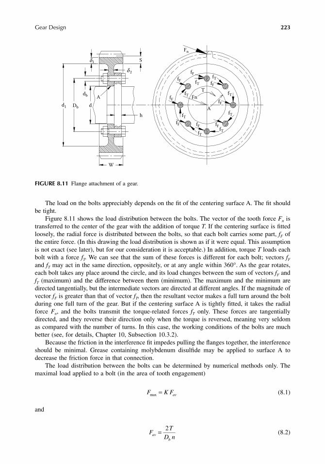
Gear Design
223
The load on the bolts appreciably depends on the fit of the centering surface A. The fit shouldbe tight.
Figure 8.11 shows the load distribution between the bolts. The vector of the tooth force
F
n
istransferred to the center of the gear with the addition of torque
T
. If the centering surface is fittedloosely, the radial force is distributed between the bolts, so that each bolt carries some part,
f
F
ofthe entire force. (In this drawing the load distribution is shown as if it were equal. This assumptionis not exact (see later), but for our consideration it is acceptable.) In addition, torque
T
loads eachbolt with a force
f
T
. We can see that the sum of these forces is different for each bolt; vectors
f
F
and
f
T
may act in the same direction, oppositely, or at any angle within 360
°
. As the gear rotates,each bolt takes any place around the circle, and its load changes between the sum of vectors
f
F
and
f
T
(maximum) and the difference between them (minimum). The maximum and the minimum aredirected tangentially, but the intermediate vectors are directed at different angles. If the magnitude ofvector
f
F
is greater than that of vector
f
T
, then the resultant vector makes a full turn around the boltduring one full turn of the gear. But if the centering surface A is tightly fitted, it takes the radialforce
F
n
, and the bolts transmit the torque-related forces
f
T
only. These forces are tangentiallydirected, and they reverse their direction only when the torque is reversed, meaning very seldomas compared with the number of turns. In this case, the working conditions of the bolts are muchbetter (see, for details, Chapter 10, Subsection 10.3.2).
Because the friction in the interference fit impedes pulling the flanges together, the interferenceshould be minimal. Grease containing molybdenum disulfide may be applied to surface A todecrease the friction force in that connection.
The load distribution between the bolts can be determined by numerical methods only. Themaximal load applied to a bolt (in the area of tooth engagement)
(8.1)
and
(8.2)
FIGURE 8.11
Flange attachment of a gear.
A
Fn
A
T
Fn
fF
fF
fF
fF
fF
fT
fTfT
fT
fT
fT
fT
fT
fF fF fF
Dbd1
h
d1
d 2
W
db
S
d
F K Favmax =
FT
D navb
= 2
9563_C008.fm Page 223 Wednesday, July 25, 2007 4:21 PM

224 Machine Elements: Life and Design
whereFav = average load (N)T = torque (N·mm)Db = diameter of the bolt circle (mm)n = number of boltsK = factor that has been calculated (see Figure 8.12)2 for the following proportions of gear:
Db/d = 1.3, W/d = 0.6, S/W = 0.25, and δ2 = h
The minimal load of a bolt
The thickness of the rim, S, in this case takes into consideration the influence of the teeth onthe rigidity of the rim:
(8.3)
whereψ = helix angle, in degreesm = module of the gearing
Equation 8.3 is exact enough when the teeth number 50 to 100. For more detailed recommen-dations, see the literature cited.7
8.3 BUILT-UP GEAR WHEELS
At diameters larger than 1500 mm (sometimes beginning at 800 mm), it is economically feasibleto make only the rim from high-strength steel (forged as a ring) and to join it (after rough machining)to a welded or cast center made of cheaper materials. The connection between the rim and thecenter may be achieved by mechanical means (bolts, rivets, or interference fit) or by welding.
Examples of welded gears are shown in Figure 8.4. The thickness of the rim for such gears δ1
is usually set equal to (5–8)m. Inside the rim, circular grooves are machined to form ribs 1 forwelding of steel plate disks. The thickness of each disk is approximately equal to 0.1 of the gearface width. In this design, butt welds are used, because they can be checked through by x-rayphotography or by ultrasonic inspection. In less important cases, in which some increased risk may
FIGURE 8.12 Factor K in Equation 8.1.
1.6 1.9 2.2 2.5 2.8 2.51.6 2.21.9 2.81.2
1.4
1.6
1.2
1.4
1.6
d1/d d1/d
K K
δ2 δ2
W = 6 W = 4
n = 12
6
6n = 12
FF
Kav
min ≈
S m= + +δ ψ1 0 22 0 009( . . )
9563_C008.fm Page 224 Wednesday, July 25, 2007 4:21 PM

Gear Design 225
be acceptable, cheaper design options shown in Figure 8.13 can be used. In this case, the weldingcan be inspected only visually. But if the welding process is well established, intermittent monitoringmay guarantee the needed quality standard.
The steel grade for the rim depends on the final heat treatment: is it case hardening, nitriding,or just quenching and tempering? But in any case such steels are poorly weldable, because theyare as a rule highly alloyed and often contain up to 0.4% carbon. This, in combination with thelarge volume of welding and necessity of subsequent cleanup, inspection, and repair of faults,makes welding very expensive. Less laborious are the mechanical connections. Figure 8.14a showsa rim of a spur gear bolted to a cast center. The centering surfaces should be tightly fitted with aminimal interference for reasons explained earlier.
FIGURE 8.13 Welded gears.
FIGURE 8.14 Connections between the rim and the center of a gear.
DDb D1 dc
Fa Fa
(a) (b) (c) (d)
wcdc
d1
W
S d1
d 2
9563_C008.fm Page 225 Wednesday, July 25, 2007 4:21 PM

226 Machine Elements: Life and Design
The rim is assembled when heated to about 100°C and bolted to the center through preliminaryholes. After the parts cool, the possible gap between the flanges should be checked with a thinfeeler gauge. If there is a gap, the parts should be pressed together, preferably using a manual orhydraulic press. When the gap is taken up, the holes can be finished, and the bolts fitted and torqued.
Concerning the size and number of bolts that attach the rim to the center, the designer is freeto choose within certain limits. Bigger bolts need thicker and wider flanges (i.e., the weight of theflanges increases), and the tightening of such bolts requires a more powerful tool. But smaller bolts,perhaps, are not strong enough to transmit the load. Comparative calculations may help the designerto choose the right size.
The load distribution between the bolts cycles with every revolution. At each moment, the mosthighly loaded bolts are those that are close to the tooth engagement zone. The maximal shear loadapplied to a bolt (provided that the centering surfaces are tightly fitted) is approximately given by3
(8.4)
whereFav and n = symbols as in Equation 8.1 and Equation 8.2a = exponent as in Figure 8.15
The minimal load is applied to a bolt that at this moment is diametrically opposite to theengagement zone and is approximately
(8.5)
EXAMPLE 8.2
The bolted spur gear shown in Figure 8.14a has the following dimensions: D1 = 794 mm, Db =740 mm, m = 8 mm, δ1 = 25 mm, δ2 = 22 mm, W = 100 mm, and number of bolts n = 24.
Calculated dimensions are S = δ1 + 0.22m = 25 + 0.22·8 = 26.8 mm (see Equation 8.3); D = D1
+ 2S = 794 + 2·26.8 = 847.6 mm; h = 0.5(D1 – Db) = 0.5(794 – 740) = 27 mm; h/S = 27/26.8 ≈ 1;S/D = 26.8/847.6 = 0.032; and W/δ2 = 100/22 = 4.55.
From Figure 8.15 for S/D = 0.03, h/S = 1, and W/δ2 = 4.55, we can find that a = 0.41. Themaximal and the minimal forces equal
Rivets may be used instead of bolts (Figure 8.14b). This connection is cheaper than the boltedjoint and quite reliable when properly designed and built.
When the rivet gets cold (after hot riveting), it shortens and presses the flanges against eachother with a large force. But for the same reason, the diameter of the rivet decreases and a smallradial gap arises between the shank of the rivet and the hole in the flanges. Thus, the strength ofthe connection is provided by friction forces in the contact region of the compressed flanges.
Tightly fitted bolts also compress the flanges, and with an even larger force, because the boltmaterial can be much stronger than that of the rivet. In addition, the fitted bolt works as a pin, sothe attainable strength of the bolt connection is much higher than a rivet connection. Besides, thequality of the bolt connection can be surely guaranteed and checked, whereas the compressive forceof the rivet can’t be measured. After all, the choice between riveted and bolted connections dependson the needed level of strength and reliability.
F F nava
max =
FF
navamin =
F F F FF
av avav
max.
min .. ; .= ⋅ = = =24 3 68
240 270 41
0 41FFav
9563_C008.fm Page 226 Wednesday, July 25, 2007 4:21 PM

Gear Design 227
Helical gears must have more rigid centers (Figure 8.14c) to decrease bending deformationunder axial force Fa. It is preferable to place the flanges so that the axial force presses them againsteach other, at least under the prevailing load (for example, with the forward motion of a ship). Itis also preferable to make the stiffening ribs so that they are exposed to compressive stress underthe prevailing load.
Figure 8.16 explains this preference. The neutral line 0–0 is placed near the wall of the disk,and under bending the rib is much more stressed than the wall. Therefore, it is highly desirable tomake the larger stress compressive.
For high-speed gears, ribs are unacceptable, because they cause unnecessary aerodynamic andfluid turbulence that result in power losses. The needed rigidity can be achieved using a thickerdisk or two thin-walled disks, perhaps with ribs between them.
In cases of bolted or riveted connections, the heat treatment of the rim (and also of the center)must be performed before assembly. This is a serious drawback of these options, because the rigidityof the separate rim is insufficient. If the teeth should be case-hardened, large deformations duringcarbonization and quenching are very difficult to avoid, and after final grinding, the thickness ofthe hard layer may be very uneven and too thin here and there. Nitriding induces relatively smallwarpage, but in built-up designs, final grinding of the teeth may be mandatory. Because the nitrided
FIGURE 8.15 Exponent a in Equation 8.4.
9 10
S
h
d 2
W
24
2 3
1 2 3 4 5 6 7 8 9 10
1
2
0.2
0.3
0.4
0.5
0.6
0.7
0.8
0.9
0.5
0.2
0.4
0.3
0.1
aa
h
S= 1
h
S= 1
h
S= 0.5
S
D= 0.01
S
D= 0.03
S
D= 0.05
D
Db
1 2 3 4 5 6 7 8
W
d 2
W
d 2
9563_C008.fm Page 227 Wednesday, July 25, 2007 4:21 PM

228 Machine Elements: Life and Design
layer is relatively thin (0.4–0.5 mm), the same problem of uneven thickness may take place hereas well. The most suitable type of surface hardening for the teeth of built-up gears is inductionhardening: first, it can be performed after assembly, when the rim is attached to a rigid center, andsecond, the induction-hardened layer is thick enough, so that the possible unevenness of its depthafter grinding is relatively small and doesn’t impair the strength of the teeth.
Gears with a shrink-fitted rim (Figure 8.14d) have the same drawbacks. The thickness of therim δ1 and the thickness of the center barrel δC can be tentatively determined as follows:4
(8.6)
whereC = center distance (mm)W = face width (mm)N1 and N2 = number of pinion teeth and gear teeth, respectively
With this calculation, the design of the gear only begins. The point is that the friction force inthe interference-fit connection (IFC) between the rim and the center may be insufficient, and theconnection may become completely spinning.
The spinning torque TS equals the torque of the friction forces:
(8.7)
wheredC = diameter of the connection (mm)W = width of connection (mm) (In fact, it can be a bit less than the face width of the gear, but
the difference usually can be neglected.)p = surface pressure in the connection (MPa)fC = coefficient of friction in the connection
In Equation 8.7 everything is clear: the dimensions are known; surface pressure p for roundparts can be calculated using the Lamé equation (see Chapter 5, Subsection 5.2.1) and, for elabo-rately shaped parts, using numerical methods. But the friction coefficient f in this connection is ofcomplex nature and deserves detailed discussion. Experiments show that under static load, f ≈ 0.28.
FIGURE 8.16 Stresses in a ribbed wall.
σmax
0 0
Disc
Ribs
δ
δ
1
1 2
1 210
5 0 001
1
=+
+ + +
=
C
N N
WC
N N mm
C
( ). ( )
.005 0 05 1+
.WC
δ
T d W p f N mmS C C= ⋅0 5 2. π
9563_C008.fm Page 228 Wednesday, July 25, 2007 4:21 PM

Gear Design 229
That means, if we substitute f = 0.28 in Equation 8.7, we attain the breakaway torque. It followsthat at some smaller load, when the entire rim is not spinning yet, there is some local micro-slipin the vicinity of the loaded tooth.
Figure 8.17 shows the very part of the shrink-fitted rim (hatched) where the local slip mayoccur. Before the tooth is loaded (Figure 8.17a), the tension forces F1 and F2 are equal, and thereare no friction forces in this connection. (Please! We are aware of the pressure forces on thecontacting surfaces, but we have intentionally omitted them.) When force Fn is applied to the tooth,the hatched part moves relative to the center and the neighboring parts of the rim in the directionof the force. At that F1 becomes greater than F2, and friction forces Ff arise at the same time.
We said “moves.” This word contains the essence of the process: where there is no motion,there is no change in the stress condition. In this case, application of load to the tooth changes thestress state of the rim, and the movement of the loaded part of the rim in the direction of the load isinevitable. Another point: the movement can be elastic. Slippage between the rim and the centeris not obligatory for the friction forces Ff to arise. Let’s consider a simple example: A solid bodyis placed on a horizontal table. Until some horizontal force is applied to the body, no friction forcesexist between the body and the table. To move the body, a horizontal force should be applied toit. If this force is less than the product of the weight of the body and the coefficient of friction, thebody doesn’t visually move. But the friction force between the body and the table exists; otherwise,why would the body not move! And if the friction force exists, there must be some kind ofdisplacement between the body and the table. This displacement may be very small, within theelastic deformations of microasperities or even within the area of molecular forces. In this case,after the external force is removed, the body will move completely back into its initial position.Experiments show that “elastic” coefficient of friction equals about one half of the coefficient ofstatic friction.
Let’s come back to the shrink-fitted toothed rim: Until the friction force lies within theboundaries of “elastic” friction, the details stay immovable relative to each other. But if the toothforce is so large that there is some zone of microslip near the loaded area, this zone travels aroundthe circumference of the gear once each revolution (along with the tooth force). The displacementduring one revolution can be very small, but with time, it accumulates. Hence, it is clear that gradualslippage in the connection of the rim with the center may occur in a working gear at a smallerforce, TS, than is needed to break the connection away at static load. Consequently, the dynamiccoefficient of friction included in Equation 8.7 should be considerably smaller.
It is also evident that the thicker the rim, the longer the local part of the rim near the loadedtooth that really participates in transmitting load to the center, and, consequently, the larger theforce that can be transmitted in the elastic range. Experiments5 have shown that at rim thicknessesof 1m, 2m, 4m, and 5m, the dynamic coefficient of friction equals 0.005, 0.017, 0.024, and 0.028,respectively. This result correlates well with the data6 that gears with a shrink-fitted rim make notroubles in service if their maximal working force can be transmitted at fC = 0.016–0.033.
Here should be underlined the peculiarity of the idea of “coefficient of friction” as appliedto this case. In Equation 8.7, it is considered that the fC value pertains to the entire surface ofthe IFC. But in reality, the force applied to the tooth executes the micromoving action only on
FIGURE 8.17 Local slippage of bandage.
(a) (b)
F2
Ff
Fn
F1 F2F1
9563_C008.fm Page 229 Wednesday, July 25, 2007 4:21 PM

230 Machine Elements: Life and Design
a small part of the rim adjoined to the loaded tooth. More distant parts are less loaded and don’tslip, although most of the connection possibly doesn’t feel the load. Therefore, in the case ofaccumulation of microslippages (as the gear rotates), the dynamic value of the friction coefficientshould be taken to calculate the strength of the rim-to-center connection in operation usingEquation 8.7.
Contact pressure p is distributed nonuniformly across the width of the gear (Figure 8.18a): itis bigger where the disks prop up the barrel of the center. The real distribution of the pressure canbe calculated by numerical methods, but in Equation 8.7 the average magnitude of the surfacepressure should be inserted. It can be found easily by representing the design (as shown inFigure 8.18b) in the form of several cylindrical bodies: rim 1, barrel 2, disks 3, and hub 4. Becausethe disks are thinner than the other parts, the modulus of elasticity of this part should be decreasedproportionally to the thickness of the disks:
whereEC = modulus of elasticity of the center material (MPa)δ2 = total thickness of the disks (mm)
Calculation of the surface pressure between parts 1 and 2 may be performed as follows:
• First, the unknown factors should be given names. For example, the surface pressurebetween parts 1 and 2 can be named p12, between 2 and 3 — p23, between 3 and 4 — p34.
• Each part should then be taken separately, and the radial displacement of each interfacesurface to be calculated using the Lamé equation.
• Now we can write three equations of joint deformations: in connections 2–3 and 3–4,the radial displacements of both contacting surfaces are even; in connection 1–2, thedifference between the displacement of the inner surface of the rim and the outer surfaceof the barrel equals the radial interference ∆.
FIGURE 8.18 Surface pressure in the shrink-fit connection between the rim and the center.
p
Ed
(a) (b)
1
2
3
4
s
d1
dh
0.5d 2d
(c)
Ed
W
d1
dc
d
E EWd C= δ2
9563_C008.fm Page 230 Wednesday, July 25, 2007 4:21 PM
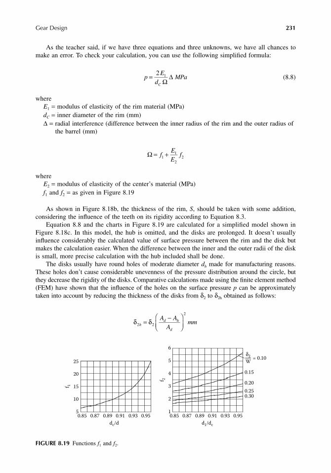
Gear Design 231
As the teacher said, if we have three equations and three unknowns, we have all chances tomake an error. To check your calculation, you can use the following simplified formula:
(8.8)
whereE1 = modulus of elasticity of the rim material (MPa)dC = inner diameter of the rim (mm)∆ = radial interference (difference between the inner radius of the rim and the outer radius of
the barrel (mm)
whereE2 = modulus of elasticity of the center’s material (MPa)f1 and f2 = as given in Figure 8.19
As shown in Figure 8.18b, the thickness of the rim, S, should be taken with some addition,considering the influence of the teeth on its rigidity according to Equation 8.3.
Equation 8.8 and the charts in Figure 8.19 are calculated for a simplified model shown inFigure 8.18c. In this model, the hub is omitted, and the disks are prolonged. It doesn’t usuallyinfluence considerably the calculated value of surface pressure between the rim and the disk butmakes the calculation easier. When the difference between the inner and the outer radii of the diskis small, more precise calculation with the hub included shall be done.
The disks usually have round holes of moderate diameter dh made for manufacturing reasons.These holes don’t cause considerable unevenness of the pressure distribution around the circle, butthey decrease the rigidity of the disks. Comparative calculations made using the finite element method(FEM) have shown that the influence of the holes on the surface pressure p can be approximatelytaken into account by reducing the thickness of the disks from δ2 to δ2h obtained as follows:
FIGURE 8.19 Functions f1 and f2.
pE
dMPa
C
= 2 1
Ω∆
Ω = +fEE
f11
22
δ δ2 2
2
hd h
d
A A
Amm= −
5
10
15
20
f 1
0.85 0.87 0.89 0.91
dc/d
0.93 0.95
25
2
10.85
3
0.87 0.89
f 2
4
5
d1/dc
0.91 0.93 0.95
6
δ2
W= 0.10
0.15
0.20
0.250.30
9563_C008.fm Page 231 Wednesday, July 25, 2007 4:21 PM

232 Machine Elements: Life and Design
whereAd = surface area of one disk (mm2)Ah = summary area of all holes in one disk (mm2)
The center of a gear made with spokes (instead of disks) has a substantial unevenness of surfacepressure around the circumference. In the span between the spokes, the barrel of the center is notsupported, and it bends; the connection between the rim and the center is weaker in these places.Therefore, it is preferable to design with disks.
The surface pressure q is the crucial factor in the reliability of the connection between the rimand the center. But the increase in pressure raises the tensile stress in the rim. Research8 has revealedthat at a tensile stress of 200 MPa, the bending strength of teeth without surface hardening isdecreased by 17 to 23%. In operating gears, the tensile stress determined by the approximate formula
(8.9)
usually doesn’t exceed 150 MPa. If the strength of the connection requires greater surface pressure,the thickness of the rim should be increased. This results both in the increase of dynamic coefficientof friction fC and the decrease of tensile stress.
Possible slippage is not the only problem one can face. Another problem is the separation ofthe rim from the center as shown in Figure 8.20. This defect is extremely harmful and may leadto quick failure of the gear. It is recommended6 that the maximal torque that doesn’t cause separationis calculated as follows:
• For the rim and center made of steel
• For the steel rim and gray cast iron center
where dp = pitch diameter of the gear.
FIGURE 8.20 Local separation of the rim from the center.
σδ
= pdC
2 1
Td p W
msepp=+
π δδ
1
10 44 9. /
Td p W
msepp=
+π δ
δ1
10 2 6 6. . /
Fn
9563_C008.fm Page 232 Wednesday, July 25, 2007 4:21 PM

Gear Design 233
EXAMPLE 8.3
Teeth numbers are N1 = 20 and N2 = 100; m = 20 mm, ψ = 9°, W = 400 mm, and output torqueT = 5 · 108 N · mm. Define the dimensions of steel rim and gray cast iron center.
Pitch diameter of the gear is
The center distance is
The root circle diameter of the teeth is
Preliminary estimate of the rim thickness from Equation 8.6 is
The inner diameter of the rim (the outer diameter of the center barrel) is
Assuming that the tensile stress in the rim should not exceed 150 MPa, the maximal permissiblesurface pressure in the connection can be found from Equation 8.9:
This pressure may be decreased because of manufacturing tolerances. Therefore, in Equation 8.7,we will insert 80% of this value, i.e., p = 7.8 MPa. The coefficient of friction fC = 0.02 (becauseδ1 = 3m)5. Thus, the permissible torque
It is only 67% of the torque to be transmitted. To increase the strength of the connection,let’s increase the rim thickness δ1 to say, 80 mm. In that case, the inner diameter of the rim isgiven by
dm N
mmp = = ⋅°
= ≈2 20 1009
2024 93 2025cos cos
.ψ
Cm N N
mm= + = ⋅°
=( )cos cos1 2
220 1202 9
1215ψ
d d m mmr p= − = − ⋅ =2 5 2025 2 5 20 1975. .
δ1
1215
10 1205
4001215
0 001 120 60 5= + + ⋅
=. . mmm
d d mmC r= − ⋅ = − ⋅ =2 1975 2 60 5 18541δ .
pd
MPaC
max
..= = ⋅ ⋅ =2 2 60 5 150
18549 791δ σ
T N mmS = ⋅ ⋅ ⋅ ⋅ ⋅ = ⋅ ⋅0 5 1854 400 7 8 0 02 3 37 102 8. . . .π
d mmC = − ⋅ =1975 2 80 1815
9563_C008.fm Page 233 Wednesday, July 25, 2007 4:21 PM

234 Machine Elements: Life and Design
and the maximal surface pressure
So, taking the same 80%, we have p = 10.6 MPa. Because the rim thickness now equals 4m,the friction coefficient can be taken as fC = 0.024. Thus, the permissible torque
Now we have to check this connection for separation:
These results are satisfying, and δ1 = 80 mm is acceptable. The barrel thickness
So the inner diameter of the center barrel
Now we can calculate the needed interference in the connection. First, we choose the thicknessof the disks: δ2 = 2 · 40 = 80 mm. Each disk has 6 holes 250 mm in diameter.
From Figure 8.19,
p MPamax .= ⋅ ⋅ =2 80 1501815
13 2
T N mmS = ⋅ ⋅ ⋅ ⋅ ⋅ = ⋅ ⋅0 5 1815 400 10 6 0 024 5 27 102 8. . . .π
Tsep = ⋅ ⋅ ⋅ ⋅+ ⋅
= ⋅π 2025 10 6 80 4000 2 6 6 20 80
11 66.
. . /. 1108 N mm⋅
δC mm= +
=1 05 0 05400
121580 85. .
d mm1 1815 2 85 1645= − ⋅ =
A mm Ad h= ⋅ = ⋅ = ⋅ = ⋅π π16454
2 125 102504
6 0 2952
6 22
. ; . 110
802 125 0 295
2 12559 3
6 2
2
2
mm
mmhδ = −
=. ..
.
dd d S mmC= + = + + + ⋅ =2 1815 2 80 20 0 22 0 009 9 1987[ ( . . )] (( . )see Equation 8 3
d
df
dd
C
C
= = =
= =
18151987
0 913 11 35
16451815
0
1
1
. ; .
.990659 3400
0 148 0 15 3 2222;
.. . ; .
δ h
Wf= = ≈ =
E MPa E MPa15
252 06 10 1 10
11 352 06
13 22
= ⋅ = ⋅
= +
. ;
..
.Ω == 18
9563_C008.fm Page 234 Wednesday, July 25, 2007 4:21 PM

Gear Design 235
Now we can obtain the maximal radial interference ∆ from Equation 8.8:
That means that the inner diameter of the rim should be less than the outer diameter of thebarrel by about 2.1 mm maximum. If the barrel is finish-machined after the rim and according toits measured inner diameter, the tolerance may be maintained within 0.3–0.4 mm. If the minimalinterference is less than the maximal by 0.4 mm (i.e., 1.7 mm instead of 2.1 mm), the minimalpressure will be, in direct proportion to the interference, 81% of the maximal.
After the design of the gear is completed (including the hub, ribs, etc.), detailed strength analysiscan be performed.
The following drawbacks of gears with shrink-fitted rims should be pointed out:
• They have much greater weight as compared to welded and bolted gears.• The rim is pretensioned, and this increases the probability of its failure.
The only benefit of such gears is their lower costs.
8.4 MANUFACTURING REQUIREMENTS AND GEAR DESIGN
Producibility considerations are an integral part of the design of anything, because it is senselessto design what can’t be produced with reasonable costs. The design of gears is in many respectsdetermined by the necessity to fasten the blank to the table of a gear-cutting machine so that it isnot deformed by the attachment and weight forces, to check the datum surfaces after the blank isattached, and to provide the required clearances (runouts) for the cutting tools.
Fastening of a large double-helical gear to the table of a gear-cutting machine is shown inFigure 8.21. The gear is attached to table 1 through pedestal 2 by pressure plate 3 and stud bolts 4.
FIGURE 8.21 Double-helical gear on the table of gear hobbing machine.
∆ Ω= = ⋅ ⋅⋅ ⋅
=p d
EmmCmax .
..
213 2 1815 18
2 2 06 101 047
15
w
2
3
5
4
1
Hob
7
8
6
9563_C008.fm Page 235 Wednesday, July 25, 2007 4:21 PM

236 Machine Elements: Life and Design
Shaft journal 6 and datum face 7 are accessible to measure radial and axial runouts. Supportingdevice 8 is meant to take the weight of the central part of the gear.
The gear in operation is not loaded by axial forces, because they get mutually balanced in theherringbone mesh. Therefore, there are no ribs between the disks (as they are shown in Figure 8.4),and the disks are pliable in the axial direction. If the central part of the gear is not supported, itsweight bends the disks elastically, and they cause the adjacent parts of the rim to deform inwardly.This results in thicker teeth in this area. When the gear is finished and installed in the horizontalposition, the disks become straight, and the rim is restored to its original shape. But the gear is outof tolerances, and it can’t work properly, because the load will concentrate on the thicker parts ofthe teeth.
In double-helical gears, the distance w between the half-gears (see Figure 8.21) needed for thehob to run out can be obtained from the equations9
whereDh = outer diameter of the hob (mm)h = entire height of the tooth (the standard height equals 2.25m)m = module of the toothing (mm)ψ = helix anglek = 5 for standard and short-addendum meshk = 5 + X for long-addendum mesh, where X is the hob displacement from its standard position
(see Chapter 7, Figure 7.12).
Figure 8.22a shows fastening of a smaller gear. Datum face 1 is resting against the machinetable through spacing ring 2. The spacing ring provides the needed clearance space for hob 3.The gear is fastened by means of disk 4 and bolts 5 that pass through holes in the gear disk. Sothe holes enable this kind of attachment, which allows the alignment of datum surfaces 1 and 6 tobe checked. The pliable disk of the gear has not been involved in the gear attachment.
Figure 8.22b shows an example of teeth cutting on a small two-rim gear. Mandrel 7 is attachedrigidly to the table of the machine, and all the misalignments are checked on the datum surfacesof the mandrel and spacer ring 8 before the work is installed. The gear is checked after finishingthe teeth.
The bigger toothing can be hobbed (hob 9) or shaped, but the smaller one can be machinedonly by shaping (shaper 10). Circular groove 11 is provided for the runout of the shaper cutter.The recommended width of the groove is as follows:9
The process of hobbing is more efficient, but it needs a wider groove, as shown in Figure 8.22c.If the teeth are case-hardened, they usually need grinding to improve their accuracy. The diameter ofthe grinding wheel 12 is greater than that of the hob, and it needs a wider clearance space (Figure 8.22d).
Figure 8.23 shows several ways of grinding teeth. Form grinders (Figure 8.23a) and conicalgrinders (Figure 8.23b) come out of contact with the work immediately after the center of thegrinder passes the face plane of the teeth. Saucer-shaped grinders (Figure 8.23c and Figure 8.23d)stay in contact with the teeth until the grinder comes completely out of the tooth space, whichrequires increased width, w, of the clearance groove.
w D h h k m when
w D h h k m
h
h
≥ − + =
≥ − ⋅ +
( ) . ( )
( ) cos t
0 1 00ψ
ψ aan ( )ψ ψwhen ≠ 00
w m≥ +4 0 66.
9563_C008.fm Page 236 Wednesday, July 25, 2007 4:21 PM

Gear Design 237
Design innovations intended to decrease the warpage of the parts during heat treatment (tospare grinding) have brought only limited success, which is satisfying in some cases, but notacceptable in others. When high accuracy of the toothing is a must, the designer is pressed toemploy any means (including separation of the gear into several parts) to ensure that grinding willbe possible. Figure 8.24a shows a kind of spline connection in which the shortened teeth of thepinion serve as splines. The connection is tightly fitted, and possible axial movement is blockedby snap ring 1.
FIGURE 8.22 Clearing space for teeth machining tools.
FIGURE 8.23 Types of grinding wheels.
Machine table
12
3
5
8
(c) (d)
1
2
4 6
7
9
1011
(a) (b)
w www
(a) (b) (d)(c)
9563_C008.fm Page 237 Wednesday, July 25, 2007 4:21 PM

238 Machine Elements: Life and Design
Figure 8.24b shows an IFC of gears with round keys (pins) 2 and screws 3 that prevent axialdisplacement in the connection. In both cases (Figure 8.24a and Figure 8.24b), the larger toothingis finished after assembly from the same datum surfaces that were used to align the smaller teeth.These connections are meant to be nonseparable.
Figure 8.24c shows a spline connection of gears with cylindrical centering surfaces. This con-nection can be dismantled, but the initial position should be marked to ensure reassembly as it was.
8.5 BEVEL GEARS
As compared with spur and helical gears, bevel gears have some peculiarities in technology anddesign. For example, in the middle of a shaft, a straight bevel gear can only be cut by a gear-shapingmachine (Figure 8.25a). Zerol and spiral bevel gears cut by a face-mill cutter require that no part ofthe gear projects from the root cone (Figure 8.25b and Figure 8.25c). In the same way that helicalgears have greater load capacity and work smoother than spur gears, Zerol and spiral bevel gears alsohave greater load capacity and work smoother than straight bevel gears. Therefore, it is worth makingbuilt-up gears (Figure 8.25d) if it is needed to use spiral bevel mesh. The separation of the gear rimalso enables carrying out the heat treatment in a rigid fixture that reduces distortion.
The thickness of the rim, δ1, usually equals the maximal tooth height. When the rim is attachedto the center by bolts as shown in Figure 8.25d, the distance between the tooth root and the threadedhole, δ2, is recommended to be not less than one third of the tooth height.
FIGURE 8.24 Assembled gears.
2
3(a) (b)
(c)
1
9563_C008.fm Page 238 Wednesday, July 25, 2007 4:21 PM

Gear Design 239
8.6 DESIGN OF TEETH
Part of the information related to the teeth has already been discussed in Chapter 7, Section 7.5(for tooth root shape, see Figure 7.13) and Section 7.7 (for tooth profile modification, see Figure 7.20).There is not much to add.
The tip thickness of a tooth, St (Figure 8.26a) depends a little on the number of teeth (seeChapter 7, Figure 7.2), but it is very much influenced by the displacement, X, of the generatingprofile (Chapter 7, Figure 7.12). Therefore, when designing gears with considerable X value, closeattention should be given to the thickness of the tooth tip. If the gears (without surface hardening)wear in service, it is recommended that St ≥ 0.5m, because the service life of this gear may belimited by the wear until the tooth tip becomes sharp. If a gear doesn’t have considerable wear, St
of ≥ 0.25m is admissible. To prevent chipping (shown in Chapter 7, Figure 7.9d), case-hardenedor nitrided teeth should have St of ≥ 2δh + (0.08 – 0.1)m, where δh is the case thickness afterfinishing. If the tooth tip is too thin, the case thickness here can be decreased by masking the topland of the teeth during the carburizing process.
The sharp edges of the tooth tip should be rounded by radius r1 ≈ 0.1m. That operation can bedone while cutting the teeth, if the hob profile has a corresponding curvature. This rounding preventsa sharp stress concentration on the edge and may be very helpful to prevent scoring. However,finish-grinding the tooth flanks may partly or completely remove these radii. They should be restoredand, when needed, polished.
The ends of a tooth should be rounded off or chamfered to make the maximal bending forcemore distant from its end. One of the possible options of chamfering is shown in Figure 8.26b.
FIGURE 8.25 Bevel gears.
FIGURE 8.26 Tooth design.
(a) (b) (c) (d)
bLe
d 1d 1
d 2
r2
r1
(a) (b) (c)
Ground faces
60°1.5 m
1 m
St
1 m
9563_C008.fm Page 239 Wednesday, July 25, 2007 4:21 PM
240 Machine Elements: Life and Design
The sharp edges of the tooth ends should be broken by chamfers or radii r2 (Figure 8.25a). Forteeth without surface hardening, it is not obligatory; deburring is usually sufficient. But for surface-hardened (case-hardened, nitrided, and such) teeth this operation must be performed before heattreatment. Usually, r2 ≈ 0.2m. These radii and the end surfaces of the teeth should not be machinedafter surface hardening, because it would diminish the bending strength of the teeth. If there is aneed for an exact ground face, it is desirable (in high-strength gears) to make it at a distance ofabout 1m from the tooth in radial or axial direction, as shown in Figure 8.25b and Figure 8.25c.
The hardened case should cover surfaces at least 1m away from the teeth ends.
REFERENCES
1. Klebanov, B.M., Design of Disc-Type Gears, Toothed and Worm Gears, collection of articles, Kolchin,N.I., Ed., Mashinostroenie, Leningrad, 1974 (in Russian).
2. Kudriavtsev, V.N., Kuzmin, I.S., and Filipenkov, A.L., Calculations and Design of Gears Handbook,Politechnika, Sanct-Petersburg, 1993 (in Russian).
3. Barlam, D.M. and Klebanov, B.M., Calculation of bolted joints of gear rims, Vestnik Mashinostroenija,No. 2, 1988 (in Russian).
4. Anfimov, M.I., Reduction Gears Design and Calculation, Mashinostroenie, Moscow, 1972 (inRussian).
5. Arai, N., Oeda, M., and Aida, T., Study of the stress at the root fillet and safety for slipping offorce-fitted helical gears, Bulletin JSME, Vol. 24, No. 198, 1981.
6. Safronov, Y.V., Up-to-date calculation of the rim thickness and the interference fit of large spur gears,Transactions of the Rostov-na-Donu Agriculture University, Rostov, 1980 (in Russian).
7. Planetary Gears Handbook, Kudriavtsev, V.N. and Kirdiashev, Y.N., Eds., Mashinostroenie, Leningrad,1977 (in Russian).
8. Lechner, G., Zahnfussfestigkeit von zahnradbandagen, Konstruktion, 19, H.2, 1967 (in German).9. Manufacturing of Gears Handbook, Taiz, B.A., Ed., Mashinostroenie, 1975 (in Russian).
9563_C008.fm Page 240 Wednesday, July 25, 2007 4:21 PM

241
9
Housings
9.1 THE FUNCTION OF HOUSINGS
Design of a housing begins when the other elements of a mechanism have been already designedin every detail: with the shafts and axles and their supports, with all dimensions of the parts andtheir motion paths. Then can be defined the dimensions of the bearing bosses, the possible locationof partings and hatches, and other elements of the housing.
This design procedure gives the impression that the housing is a kind of envelope and can bemade of any material. This impression is false; a housing is just one of the components of amechanism, as the shell is an integral part of a tortoise’s skeleton. Without this part the mechanismdoesn’t exist. This is the difference between a housing and a guard; the latter is just to isolate themechanism from the surroundings.
The housing is almost always the biggest part of a mechanism. It is usually made as a closed box,so that the rest of the parts are mounted inside it. In this respect, the housing also serves as a guard.
The housing is most often (not always) the fixed part of a mechanism that serves to attach itto some foundation or substructure or to another unit.
Notice that
fixed
always means immovable relative to something. For example, let’s consider theswinging mechanism of a crane shown in Figure 9.1. Platform 1 is set in motion by pinion 2, drivenby electric motor 3, through worm gear 4. Pinion 2 revolves around gear 5 that is bolted to base 6,which is, in turn, bound to the ground (possibly through a movable platform, like the chassis of avehicle). If the entire crane is considered as a mechanism, the fixed part is base 6. If the mechanismis worm gear 4, its housing 7 is the fixed part relative to the worm, the gear, and the bearings.
Though the mobility or immobility of the housing may be just a matter of definition, itsmovement in space should be taken into consideration. When the housing moves, all the parts ofa mechanism (including the oil) are exposed to inertia forces, which can essentially change theload of the parts and the lubrication conditions.
It is appropriate to mention here that gravitation is also applied to all the parts, and it shouldbe taken into account. For example, a purposeful increase in weight of a part may change profitablythe direction and value of a load vector.
Serving as a guard, the housing isolates the mechanism from the surroundings to createconditions inside that are comfortable for the mechanism. On the other hand, the housing isolatesthe surroundings, including the personnel, from the mechanism, so that we are protected fromhearing the noise and from being sprinkled with hot oil; besides, we can’t easily put our fingersinto it. This is an important function of the housing; nevertheless, it is not an envelope but one ofthe parts of a mechanism. Therefore, with respect to stress and strain analysis, the housing deservesattention no less than any other machine element. The problem is that housings usually have acomplex spatial shape. It can be analyzed by “engineering methods” (i.e., traditional analyticalmethods) very approximately, under simplifying assumptions. This method, however, requires acertain level of experience and feeling of how the housing deforms under load; otherwise, thesimplifications may be done incorrectly, and the results of the calculation may be far from satis-factory. More exact information of the stresses and elastic deformations of the housing can beobtained using the finite element method (FEM). But this method also requires some simplificationsin most cases, for example, when defining the boundary conditions in bolted joints, when presettingthe load distribution in bearings, and others. The choice of appropriate simplifications is a matterof experience with the machine elements and awareness of computer program subtleties.
9563_C009.fm Page 241 Wednesday, July 25, 2007 4:23 PM

242
Machine Elements: Life and Design
The housing is an assembly basis for the rest of the parts and units of the mechanism. Therefore,it should meet some obligatory requirements:
1. Because the mechanism is assembled inside the housing, the latter must be designedso as to enable assembly operations and the control of parameters to be checked afterassembly. That means, the housing should have partings or sufficiently sized openingsthat enable convenient assembly and control of the mechanism. Sometimes the mech-anism must be periodically inspected while in service to check the condition of wearingparts (like gear teeth or bearings). For this purpose, the housing should be providedwith inspection hatches in needed places. For example, hatch 8 in Figure 9.1 enablescontrol of the tooth contact patch during assembly, visual inspection of the teeth inservice, and measurement of backlash in the worm mesh. The hatches may reduce thestrength and rigidity of a housing; therefore, their dimensions should not be too largebut enough to enable the actions they are made for. In relatively small mechanisms, itmay be preferable to dismantle the mechanism for inspection and in that way avoid theinspection hatches.
2. As was said, the housing as an ordinary member of a mechanism should have exactdimensions where it is in contact with other parts. This accuracy should be achieved inproduction and then remain within admissible limits while the housing is exposed tomechanical and temperature influences. Figure 1.1 (see Chapter 1) shows frame 4, whichserves as a housing (not closed in this case). Insufficient rigidity of the frame has led toincrease in the distance between the lugs. Consequently, the parallel link mechanismdoesn’t operate properly and the weight has fallen. Figure 1.5e (see Chapter 1) showsthe elastic deformations of a gear housing that lead to misalignment of the shafts.
Dimensional stability of the housing is a mandatory requirement, as for every othermember of a mechanism. Change in dimensions can relate to elastic and plastic defor-mations under load or to thermal expansion, or it may be caused by structural changesin the material. Metals, with their high strength, high modulus of elasticity, and stablestructure (after appropriate heat treatment), are preferable to other materials. Therefore,housings are almost always made from metals.
FIGURE 9.1
Swinging mechanism of a crane.
1
2
3 7
5 6
48
9563_C009.fm Page 242 Wednesday, July 25, 2007 4:23 PM

Housings
243
3. In addition, some other requirements may be important, such as• Heat conductivity of the housing material (to enable more effective heat extraction
from inside to outside)• Ability to damp noise and vibrations• low weight• Ability to withstand aggressive environments, such as seawater, and others, which
can be achieved on any material by suitable coatings
9.2 MATERIALS FOR HOUSINGS
Because housings are intricately shaped, they are mostly cast, and usually only the surfaces that fitto other components are machined. One of the most widespread materials is gray iron. It has goodcastability and machinability, increased (as compared with construction steels) corrosion resistance,and good wear resistance (because it is “impregnated” with graphite). Good damping capacity enablesit to reduce the noise and vibrations created in the working mechanism. But gray iron is brittle andsensitive to overload and impact load; therefore, it is not recommended in dangerous applications,for example, in devices intended for transportation of foundry ladles filled with molten metal.
The wall thickness of a gray iron housing depends on several variables, including stress,achieving adequate stiffness, method of casting, etc., and can be approximately obtained fromFigure 9.2
1
, curve 1. In this figure,
N
is the equivalent dimension of the casting which is given by
where
L
is the length (the largest dimension of the casting),
W
, the width, and
H
, the height of thecasting, all in meters.
The recommendations given in Figure 9.2 are average. Depending on the complexity of thecasting, technology used, and the temperature of the metal charged, the minimal wall thicknessmay be somewhat lesser or greater. For example, if a large foundry ladle feeds into several molds,the metal will cool slightly during the process of charging. So the wall thickness should be somewhatgreater to be satisfactory for the last of the molds. In any case, the design of the casting should bediscussed with the manufacturers and submitted for their approval.
E
XAMPLE
9.1
The housing is 3000 mm long, 1500 mm wide, and 1000 mm high.
W
=
1/3 (2 · 3
+
1.5
+
1)
=
2.83 m,and the practically feasible wall thickness of cast gray iron is about 20–22 mm. The strength andthe rigidity of the housing should be checked afterward, and if they are insufficient, they can beincreased mainly by adding ribs or, possibly, by increasing the wall thickness.
FIGURE 9.2
Practically feasible wall thickness of a casting.
N L W H= + +13
2( )
0 1 2 3 4
N (meters)
Min
imal
wal
l th
ick
nes
s (m
m)
10
0
30
20 1
2
9563_C009.fm Page 243 Wednesday, July 25, 2007 4:23 PM
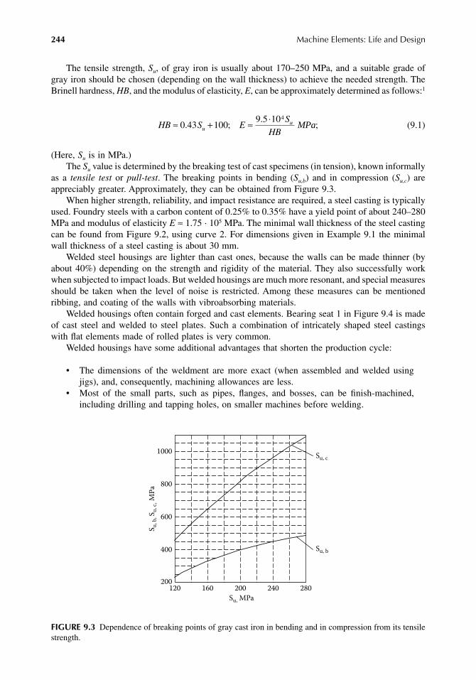
244
Machine Elements: Life and Design
The tensile strength,
S
u
, of gray iron is usually about 170–250 MPa, and a suitable grade ofgray iron should be chosen (depending on the wall thickness) to achieve the needed strength. TheBrinell hardness,
HB
, and the modulus of elasticity,
E
, can be approximately determined as follows:
1
(9.1)
(Here,
S
u
is in MPa.)The
S
u
value is determined by the breaking test of cast specimens (in tension), known informallyas a
tensile test
or
pull-test
. The breaking points in bending (
S
u,b
) and in compression (
S
u,c
) areappreciably greater. Approximately, they can be obtained from Figure 9.3.
When higher strength, reliability, and impact resistance are required, a steel casting is typicallyused. Foundry steels with a carbon content of 0.25% to 0.35% have a yield point of about 240–280MPa and modulus of elasticity
E
≈
1.75 · 10
5
MPa. The minimal wall thickness of the steel castingcan be found from Figure 9.2, using curve 2. For dimensions given in Example 9.1 the minimalwall thickness of a steel casting is about 30 mm.
Welded steel housings are lighter than cast ones, because the walls can be made thinner (byabout 40%) depending on the strength and rigidity of the material. They also successfully workwhen subjected to impact loads. But welded housings are much more resonant, and special measuresshould be taken when the level of noise is restricted. Among these measures can be mentionedribbing, and coating of the walls with vibroabsorbing materials.
Welded housings often contain forged and cast elements. Bearing seat 1 in Figure 9.4 is madeof cast steel and welded to steel plates. Such a combination of intricately shaped steel castingswith flat elements made of rolled plates is very common.
Welded housings have some additional advantages that shorten the production cycle:
• The dimensions of the weldment are more exact (when assembled and welded usingjigs), and, consequently, machining allowances are less.
• Most of the small parts, such as pipes, flanges, and bosses, can be finish-machined,including drilling and tapping holes, on smaller machines before welding.
FIGURE 9.3
Dependence of breaking points of gray cast iron in bending and in compression from its tensilestrength.
HB S ES
HBuu≈ + ≈ ⋅
0 43 1009 5 104
. ;.
;MPa
200
400
600
800
1000
120 160 200 240 280
Su, c
Su, b
Su
, b, S
u, c
, MP
a
Su, MPa
9563_C009.fm Page 244 Wednesday, July 25, 2007 4:23 PM

Housings
245
• Oil ducts can be easily welded as an integral part of the welded structure (see Chapter 6,Figure 6.39b); the incorporated pipe can be bent and bifurcated if needed, whereas in acast housing the oil duct must be drilled after the casting is machined (Chapter 6,Figure 6.39a) and obviously must be straight.
When light weight is a mandatory requirement, aluminum and magnesium alloys are used forthe housings. The specific weight of aluminum alloy is about one third, and of magnesium alloy,about one quarter, that of gray cast iron. So if the minimal wall thickness is limited by the castingtechnique only, the gain in weight is great. But the strength, rigidity, and temperature deformationsof housings are always under consideration. The comparison characteristics of mechanical properties(yield point
S
y
, modulus of elasticity
E
) and linear expansion factors
α
of rolled and cast steels,gray iron, aluminum and magnesium cast alloys are given in Table 9.1. As one can see, mechanicalproperties of aluminum alloy can be very close to those of gray iron, but it is inferior to gray ironin wear resistance. Therefore, friction should be avoided in the design of an aluminum housing. Inparticular, all the seats of rolling bearings should be reinforced by steel sleeves as shown inFigure 6.19a, Figure 6.19c, and Figure 6.23 of Chapter 6. The sleeve should be tightly fitted, andthe interference value should prevent joint separation at the highest service temperature. The sleeveis exposed to a turning moment, just as the bearing rings are (see Chapter 6, Subsection 6.2.5),and may rotate. This rotation may be prevented by bolts (as in Figure 6.19a) or pins (2 in Figure 6.23,Chapter 6). Otherwise, the interference should be increased. The needed value of it can be calculatedin accordance with recommendations given in Chapter 6, Subsection 6.2.5.
FIGURE 9.4
Fragment of a welded gear housing.
TABLE 9.1Mechanical Properties of Some Housing Materials
Material
S
y
(Mpa)
E
(Mpa)
α
1/
°
C
Rol
led
plat
e
SAE 1020 annealed 250 2.00 · 10
5
12.2 · 10
−
6
SAE 4130 normalized 490 2.00 · 10
5
12.2 · 10
−
6
Hardox 400, Creusabro 4000 900 2.06 · 10
5
12.2 · 10
−
6
Cas
ting
Cast steel 240–260 1.70 · 10
5
12.2 · 10
−
6
Gray iron Su
=
170–250 (0.9-1) 10
5
See Eq. (9.1)
(10–12) · 10
−
6
High-duty cast iron 320–370 1.70 · 10
5
12 · 10
−
6
Aluminum alloys 150–180 0.72 · 10
5
(20–26) · 10
−
6
Magnesium alloys 80–120 0.45 · 10
5
(26–30) · 10
−
6
A
Section A-A
1
A
9563_C009.fm Page 245 Wednesday, July 25, 2007 4:23 PM

246
Machine Elements: Life and Design
The end covers of bearings that transmit axial force from the bearing to the housing (such asthose shown in Figure 6.8f, Figure 6.8h, Figure 6.8i, Figure 6.11e, Figure 6.11f, and Figure 6.22— see Chapter 6) should be made of strong, wear-resistant materials.
If the housing is split through the axes of the gears, elements of axial fixation of the bearingsare sometimes installed in circular grooves (for example, ring and cover in Figure 6.8c, cup andcover in Figure 6.8f — see Chapter 6). These parts can’t be installed with interference fit becauseit would impede the connection of two halves of the housing. So, when the outer ring of the bearingrotates (see Chapter 6, Subsection 6.2.5), it may also drag the fixing elements into rotation. (Rotationof the cover can be observed.) And if the housing or the fixing elements are made of light metal,their intensive wear is unavoidable.
The threaded connections in light-metal housings are usually made using studs with interference-fit thread of the tap end. The length of this end should be about (1.5–2.0)
d
(Figure 9.5a) dependingon the strength of the stud and of the housing materials. When needed, the diameter of the tab endcan be increased as shown in Figure 9.5b. This stud is provided with hexagonal part 1 to preventtorsion of the stud shank by a heavy torque needed to assemble the tight thread.
When a standard size, reusable thread in the light-metal housing is needed, the housingwall should be reinforced by threaded inserts (2 in Figure 9.5c) made from corrosion-resistantsteel and installed fast in the housing, using an insert with interference-fit outer thread, a self-tapping insert, a keyed insert, or by application of the appropriate kind of anaerobic compoundsuch as Loctite.
All these requirements and recommendations may be surplus if the mechanism is low-loadedor designed for short-term applications.
Irrespective of the material or manufacturing method, the housing needs heat treatment torelieve internal stresses. In cast housings, these stresses are caused by uneven solidification of thecasting. The more massive volumes harden later, and, as they become cooler and decrease in theirdimensions, they pull their thinner neighbors that are already hard and rigid and can’t deform thatmuch. This struggle between the neighbors, each pulling in a different side, may result in a crack,or, at best, the internal stress remains in the casting.
Avoidance of massive volumes in the casting is very desirable but not always possible. Anyway,unnecessary metal should be removed from local bosses, and the transition from wall to boss shouldbe made smooth with generously rounded corners.
Another method to prevent cracks in castings is to make pliable configurations. Figure 9.6shows the spoked wheels, in which spokes 1 harden first, and hub 2 and rim 3, later. Dependingon which of them, rim or hub, hardens later, the spokes may appear compressed or tensioned. Toprevent high shrinkage stresses, the spokes can be made curved (Figure 9.6a) or slanted (Figure 9.6b).
FIGURE 9.5
Reinforcement of threads in light-metal housings.
(a) (b)
2
(c)
1
2d
d
9563_C009.fm Page 246 Wednesday, July 25, 2007 4:23 PM

Housings
247
In these cases, the difference in the shrinkage of the rim and the hub leads to small bendingdeformations of the spokes.
Very large wheels are often made with a slit hub (Figure 9.6c). Such a wheel is slide-fitted tothe shaft, and the needed press fit is achieved from massive rings mounted on the ends of the hubwith a great interference. This design is archaic. Nowadays such wheels are welded of low carbonsteel, and the problems of possible cracking are avoided.
The mechanism of deformation of welded housings is similar to that described previously. Thewelded components that are straight before welding (Figure 9.7a) are pulled by the weld whilegetting cold and become deformed as shown in Figure 9.7b.
The internal stresses are quite high, and, in course of time, the material little by little gets freeof them owing to continuous sluggish plastic deformation in the crystals. Because the housings arerelatively large and thin walled, their warpage might be unacceptably large. Therefore, to relievethese internal stresses, housings are usually heat-treated before final machining. The heat treatmentconsists of exposure of the casting (or the weldment) to high temperature for several hours followedby slow cooling within the oven (to prevent formation of new internal stresses because of nonuni-form cooling). The temperatures depend on the kind of material and approximately range from 550to 650
°
C for ferroalloys and from 170 to 250
°
C for aluminum and manganese alloys. At thesetemperatures, the material becomes pliant, so that the internal stresses deform it in a relatively shorttime and disappear almost completely. The same process improves the microstructure of thematerial, and cast materials undergo aging.
The cast and forged elements used for welded housings usually should undergo stress-relievingheat treatment before welding in order to decrease deformations during heat treatment of the entireweldment.
FIGURE 9.6
Prevention of cracking in the spoked wheels.
FIGURE 9.7
Deformation of welded parts.
(a) (c)(b)
23
1
(a)
(b)
9563_C009.fm Page 247 Wednesday, July 25, 2007 4:23 PM
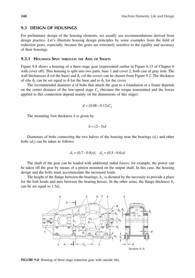
248
Machine Elements: Life and Design
9.3 DESIGN OF HOUSINGS
For preliminary design of the housing elements, we usually use recommendations derived fromdesign practice. Let’s illustrate housing design principles by some examples from the field ofreduction gears, especially, because the gears are extremely sensitive to the rigidity and accuracyof their housings.
9.3.1 H
OUSINGS
S
PLIT
THROUGH
THE
A
XES
OF
S
HAFTS
Figure 9.8 shows a housing of a three-stage gear (represented earlier in Figure 6.15 of Chapter 6with cover off). This housing is split into two parts, base 1 and cover 2, both cast of gray iron. Thewall thicknesses
δ
(of the base) and
δ
1
(of the cover) can be chosen from Figure 9.2. The thicknessof ribs
δ
2
can be set equal to
δ
for the base and to
δ
1
for the cover.The recommended diameter
d
of bolts that attach the gear to a foundation or a frame dependson the center distance of the low-speed stage
C
L
(because the torque transmitted and the forcesapplied to this connection depend mainly on the dimensions of this stage):
The mounting foot thickness
h
is given by
Diameters of bolts connecting the two halves of the housing near the bearings (
d
1
) and otherbolts (
d
2
) can be taken as follows:
The shaft of the gear can be loaded with additional radial forces; for example, the power canbe taken off the gear by means of a pinion mounted on the output shaft. In this case, the housingdesign and the bolts must accommodate the increased loads.
The height of the flange between the bearings,
h
1
, is dictated by the necessity to provide a placefor the bolt heads and nuts between the bearing bosses. In the other areas, the flange thickness
h
2
can be set equal to 1.5
d
2
.
FIGURE 9.8
Housing of three-stage reduction gear with outside ribs.
d CL= −( . . )0 08 0 12
h d= −( )2 3
d d d d1 20 7 0 8 0 5 0 6= − = −( . . ) ; ( . . )
1
34
CL
4 6
5
3
7
2d1
d6
R
A
2
h1
h
d
d4
d3
h2
d5
d2
DD1
d1 d 2
A
Section A-A
d
d1
9563_C009.fm Page 248 Wednesday, July 25, 2007 4:23 PM

Housings
249
The outer diameter
D
1
of the bearing bosses 3 can be set equal to
where
D
=
outer diameter of the respective bearing (mm).The diameters of bolts
d
3
that attach the bearing caps to the housing can be obtained from theequation
For the sake of convenience in service, the diameter of all the bolts,
d
3
, should be the same(but it is not a must); this may require some increase in diameter
D
1
of smaller bearing bosses.These bolts are exposed to the axial force created in the gear mesh and in the bearings. Theircalculation for strength should take into consideration that the axial force is distributed nonuni-formly between the bolts, and the maximum-to-average ratio may be about 5 (see Chapter 6,Example 6.6).
The position of the base and the cover relative to each other is fixed by two pins; their diameter
d
4
≈
0.8d2. In addition, the housing is provided with lifting eyes 4; drain hole d5 (of about 16–42 mmin diameter, depending on the housing size), oil indicator 5, opening 6 for a breather, and jackscrewholes 7 (for disassembly).
It is desirable to place the breather in the highest point of the housing; otherwise, part of theinner volume would not be ventilated, and the steam condensate would remain in the housing. Thismay cause severe corrosion in nonventilated areas during warehousing.
The jackscrew hole 7 has been made in this case on the lower flange. If it is made on the upperflange, it should be closed with a greased plug to prevent filling with debris.
The relative positions of the wall and the bearing boss are important both for housing strengthand bearing alignment. The minimal bending stress of the wall is achieved when it is placedsymmetrically about the radial reaction of the bearing, as shown in Figure 9.9a. If, in addition, the
FIGURE 9.9 Deformations of the shaft and the bearing bosses.
D D1 1 25 10= +. mm
d D3 0 04 4= +. mm
(b) (c)(a)
(e)(d)
9563_C009.fm Page 249 Wednesday, July 25, 2007 4:23 PM

250 Machine Elements: Life and Design
bending deformations of a shaft are negligible, this arrangement is the best. If the shaft is pliableunder load, the location of the wall relative to the boss shown in Figure 9.8 and Figure 9.9b is theworst (if the bearings are sensitive to misalignment). In this case, not only is the wall exposed tobending but also the deformations of the shaft and the boss are oppositely directed. The wall locationshown in Figure 9.9c and Figure 9.10 is preferable when the shaft is pliable, because the deformationof the boss decreases the bearing misalignment.
Blocking the boss deformation by a central rib (Figure 9.9d) is a wrong idea because thisworsens the load distribution in the bearing (see Figure 6.21c and Figure 6.21d). The ribs shouldbe placed as shown in Figure 9.9e.
The housing design shown in Figure 9.10 offers some additional advantages, besides thefavorable deformation of the bearing bosses: the walls become more rigid, and the volume of theoil reservoir increases. Above the bearing boss can be made a trap for the oil splashed by the gearsso as to surely lubricate the bearing, as shown in Figure 7.26b (Chapter 7). But it also hasdisadvantages as against the version in Figure 9.8: the casting is more complicated, and the cleaningand painting of the inner surfaces of the casting is more difficult.
9.3.1.1 Design of Mounting Feet
The mounting feet are intended for attachment of the housing to a base or foundation. They are themost heavily stressed elements of the housing. The initial state of the mounting foot (before loading)is shown in Figure 9.11a. When there is a tensile load applied to the wall, the mounting foot isbent in two directions: crosswise (Figure 9.11b) and lengthwise (Figure 9.11c). This deformationinvolves the bending of the adjoined parts of the walls. If the mounting foot is thin and pliable,the load is not distributed along its length, but mostly transferred in the vicinity of the bolt. Thestresses in this area may be increased considerably and result in a failure of the wall.
The thicker the mount foot, the less it bends in both directions, and the longer part of the wallis involved effectively in the load transfer between the wall and the bolt. This decreases both thebending stress and the tensile stress in the wall. Bending deformations are further reduced by addingribs (Figure 9.11d) that also make the loading mode of the bolt closer to centric.
The maximal strength and rigidity of the mounting foot is attained in the design shown inFigure 9.11e. Here, the bolt is put into a recess, and its loading can be considered as centric.The bending of the mounting foot is relatively small. The dimensions of the recess should beas small as possible, but not less than needed to put the bolt in and then to turn it by somekind of wrench. The tolerances of the castings or weldments must take all these requirementsinto account.
FIGURE 9.10 Housing of three-stage reduction gear with inside pockets.
A
A Section A-A
9563_C009.fm Page 250 Wednesday, July 25, 2007 4:23 PM

Housings 251
9.3.1.2 Design of Lifting Elements
Load lifting must be thoroughly planned and calculated. First, the location of the center of gravity(CG) should be defined, and the lifting elements must be so located as to prevent the loadoverturning. The quantity of lifting points depends on their possible location relative to the centerof gravity and on the practicable load capacity of the elements used. For small- or middle-sizedunits, one or two lifting points may satisfy the need. In large and heavy units four or even morelifting points may be needed, and special instructions should be worked out to use them properly.
It is preferable to use elements that have standard dimensions and prescribed permissible load,such as lifting hooks (items 7 and 8 in Figure 9.12) and eyebolts (item 8 in Figure 9.14). Theothers, such as lifting lugs cast with the housing (item 4 in Figure 9.8), hatch covers with a lug(item 8 in Figure 9.13), and the like, must be carefully assessed for strength with safety factorsgenerally accepted for load lifting devices.
Typical safety factors for lifting devices, such as those mentioned, may range up to 6 or evenhigher. These high margins are necessary to allow for manufacturing variations (undetected porosityin castings), environmental deterioration, normal wear, etc., and even possible misuse. It is verycheap insurance and allows peaceful sleep for the designer!
All the strapping elements must be controlled in production. For example, the lifting eyes andhooks attached to the wall of the housing may fail if the wall thickness in this area is thinner thanindicated in the drawing (this may occur owing to displacement of the mold core).
Lifting eyes cast with the housing (item 4 in Figure 9.8) are usually twice as thick as the wall.The hole diameter d6 ≈ 3δ1, and R = d6.
9.3.2 HOUSINGS SPLIT AT RIGHT ANGLE TO THE AXES OF THE SHAFTS
Examples of such design are shown in Figure 7.30, Figure 7.31 (Chapter 7), and Figure 10.26 (Chapter10). In the first two cases, the gears are with vertical shafts. The housing of the bevel-planetary gear
FIGURE 9.11 Mount feet design.
(a) (b) (c)
A A
(d) (e) Section A-A
9563_C009.fm Page 251 Wednesday, July 25, 2007 4:23 PM

252 Machine Elements: Life and Design
FIGURE 9.12 Housing of two-stage gear shown in Figure 7.31 (Chapter 7).
FIGURE 9.13 Bevel gear in nonsplit housing.
1
4
2
35
6
7
8
A
Section A-A
1
3
8 5
6
7
2
4
17
12 13
20 21
19 18
22
A
11 9 10
15
14
16
9563_C009.fm Page 252 Wednesday, July 25, 2007 4:23 PM

Housings 253
from Figure 7.31 is shown in Figure 9.12. It consists of base 1, upper housing 2, and cover 3. Parts1 and 2 are centered through fixed annulus 4. Flange 5 is intended for mounting an electric motor.Inspection hatch 6 is necessary during assembly to check the contact pattern in the bevel gear. Itis also useful in service to periodically inspect the bevel gear teeth.
The housings split at a right angle to the axes offer a number of advantages:
• The geometry of the bearing seats is more exact.• The connection of two parts of the housing is not cut by the bearings, and therefore, it
can be made lighter and stronger.• The joint surface is flat and continuous, and its leakproofness can be more easily achieved.
What kind of housing design is preferable? Most general-duty gears have housings split on ahorizontal or slightly slanted plane. The reason is clear: the foundation or mounting frame the gearis attached to is usually horizontal. If there is something wrong with the gear, you take off theupper part of the housing (the cover), and the lower part (the base) with the oil remains attachedto the foundation. So you can inspect the whole gear mechanism, replace the damaged parts, thenattach the cover and tighten the bolts. The oil filling as well as the alignment of the input andoutput shafts with other units remain unchanged and don’t need any additional work.
9.3.3 NONSPLIT HOUSINGS
Small-sized gears are often made in nonsplit housings (where possible). Figure 9.13 shows a bevelgear of such kind. Gear 1 with its shaft and bearings is installed through openings closed withcovers 2 and 3. (Only one cover is enough to allow assembly of the unit. However, a second coveris provided to enable assembly with an oppositely directed output shaft without any change indetails.) This housing also has inspection hatch 4, breather 5, oil gauge 6, and oil drain 7. Theinspection hatch is needed during assembly to check the contact patch of the teeth and to adjustproperly the axial positions of both the gear and the pinion.
A worm gear in a nonsplit housing is shown in Figure 9.14. Gear 1 with its shaft and bearingsis installed through openings closed with covers 2 and 3. This housing is provided with an inspection
FIGURE 9.14 Worm gear in nonsplit housing.
8
A
B
B
A
Section B-B Section A-A
1
2
3
4
6
5
7
9563_C009.fm Page 253 Wednesday, July 25, 2007 4:23 PM
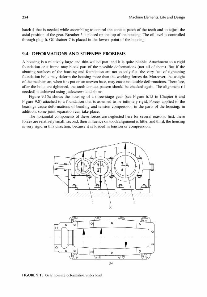
254 Machine Elements: Life and Design
hatch 4 that is needed while assembling to control the contact patch of the teeth and to adjust theaxial position of the gear. Breather 5 is placed on the top of the housing. The oil level is controlledthrough plug 6. Oil drainer 7 is placed in the lowest point of the housing.
9.4 DEFORMATIONS AND STIFFNESS PROBLEMS
A housing is a relatively large and thin-walled part, and it is quite pliable. Attachment to a rigidfoundation or a frame may block part of the possible deformations (not all of them). But if theabutting surfaces of the housing and foundation are not exactly flat, the very fact of tighteningfoundation bolts may deform the housing more than the working forces do. Moreover, the weightof the mechanism, when it is put on an uneven base, may cause noticeable deformations. Therefore,after the bolts are tightened, the tooth contact pattern should be checked again. The alignment (ifneeded) is achieved using jackscrews and shims.
Figure 9.15a shows the housing of a three-stage gear (see Figure 6.15 in Chapter 6 andFigure 9.8) attached to a foundation that is assumed to be infinitely rigid. Forces applied to thebearings cause deformations of bending and tension compression in the parts of the housing; inaddition, some joint separation can take place.
The horizontal components of these forces are neglected here for several reasons: first, theseforces are relatively small; second, their influence on tooth alignment is little; and third, the housingis very rigid in this direction, because it is loaded in tension or compression.
FIGURE 9.15 Gear housing deformation under load.
123
δ3
(a)
(b)
δ2 δ1
9563_C009.fm Page 254 Wednesday, July 25, 2007 4:23 PM

Housings 255
If shafts 1, 2, and 3 were symmetrically loaded and the bearing forces were equal, and if thehousing design was also symmetrical, then displacements δ1, δ2, and δ3 would be equal on bothsides of the housing and would not cause any misalignment of the gear teeth. But from Figure 6.15(Chapter 6), it is obvious that the load is distributed nonuniformly between the two bearings ofeach shaft, so the housing deformations (as well as the deformations of the bearings; see Chapter 6,Subsection 6.2.7) result in error in parallelism of the shafts and misalignment of the teeth.
Figure 9.15a makes clear the importance of the bolts that connect the two halves of the housing.They should be strong enough and properly tightened to prevent joint separation.
Axial forces applied to the teeth in helical gears may increase the difference in the bearingreactions, because they add bending moments to the shafts. Consequently, misalignment of theteeth may be increased. Therefore, in large gears, in which the attainment of needed teeth alignmentunder load presents difficulties, double-helical (i.e., herringbone) mesh is favored (for its symmetryand lack of axial forces outside the mesh).
In smaller gears, the axial forces are less harmful, and helical gears are mostly in use. Figure 9.15bshows the axial forces in a gear from Figure 6.15 (Chapter 6) and the respective deformations of thehousing. These deformations may be harmful for bearings with adjustable end play, such as angularcontact ball bearings (Figure 6.4b in Chapter 6) and tapered roller bearings (Figure 6.4f in Chapter 6).
Deformations of the housing are shown exaggerated in Figure 9.15, but even small deformationscan’t be neglected. In Chapter 7, Example 7.6, tooth misalignment of only 10 mm led to noticeablyuneven load distribution across the face of the gear (KW = 1.14).
Deformations caused by axial forces have been measured on two-stage helical reduction gears.2
The maximal increase in distance between the side walls has been found as large as 0.10–0.15 mmand 0.13–0.22 mm for gears with a total center distance of 500 mm and 650 mm, respectively.
9.5 HOUSING SEALS
To prevent communication between the inside of the housing and the surroundings, all locationswhere this communication may take place must be sealed. The consequences of seal failuredetermine the requirements of the seal specification. For example, if an oil-lubricated mechanismworks in a clean room, the ingress of air inside the housing is admissible. Leakage of oil from thehousing is unpleasant, but if it is one drop a day, it can be bearable.
If such a mechanism works in a food production line and has contact with food, no oil leakagefrom the housing can be permitted, and no ingress of the product into the housing can be welcomedeither. The same can be said about a submerged mechanism: oil leakage pollutes the water, andwater ingress into the housing is likely to damage the mechanism.
The most stringent sealing requirements are necessary if the housing contains substances thatare dangerous for the environment or personnel. In these cases, more than one stage of sealing isused as a rule, with control and alarm devices after each stage.
A principal distinction should be made between the sealing of rigid connections and that ofmovable connections. As the former can be usually made very reliable, the latter have more or lessreliable solutions for easy applications, but still need the trial-and-error method where the workingconditions are complicated. In the following subsections are discussed features of some sealingmethods and devices.
9.5.1 SEALING OF RIGID CONNECTIONS (STATIC SEALS)
These connections can be divided into two groups:
Group 1. Connections in which an exact relative position of the connected parts must beensured: This requirement is indispensable with reference to parts that are elements of amechanism; in other words, the mechanism can’t work without any of these parts. Among
9563_C009.fm Page 255 Wednesday, July 25, 2007 4:23 PM

256 Machine Elements: Life and Design
them can be mentioned connection of housing parts that contain supports of shafts,connection of bearing cap to the housing, provided that the cap adjusts the axial positionof the shaft or the axial play of the bearing, and so on.
Group 2. Connection of parts that are not involved in the kinematics of the mechanism:Such parts, like covers of inspection hatches, blind flanges of manufacturing holes, pipejoints, etc., can be positioned with greater tolerances relative to the housing, providedthat their displacement doesn’t impede their function. That means, for example, thehatch cover must close up the opening at all tolerances, the pipe flange should be attachedso that the tube is coaxial (within reasonable limits) with the duct in the housing, andthe like.
Parts that belong to Group 1 must be in direct contact (metal-to-metal) with each other overtheir joint surfaces. These surfaces must be machined to tight tolerances (and sometimes a finesurface finish) to keep unchanged the precise geometry of the parts after assembly operations.
If the contact between two joint surfaces is imperfect, the parts become deformed whiletightening the bolts, and their exactness is impaired. But this is not the only problem. Afterdismantling and reassembly of such parts, their deformation will be different than before, dependingon the sequence of tightening the bolts, tightening forces and residual deformation of the joinedparts. Therefore the geometry errors after reassembly may become increased even if the parts havebeen machined jointly (i.e., while assembled), and each reassembly may give different values ofthese errors.
It is very difficult to achieve leakproofness in plain metal-to-metal contact: the surfaces mustbe very exact, very smooth, and tightly pressed against each other over the entire surface. (Thelatter is not always easily achieved, because the bolted connection is “spotty”; see Chapter 2, Section2.2.) Therefore, the joints are usually sealed with special compounds which are initially liquid.These compounds don’t hinder the metal-to-metal contact, but they fill up all the undulations ofthe surfaces and later on, after the bolts are tightened, they become in small gaps semiliquid orrubberlike, vulcanized to the joint surfaces. In that way are eliminated excessive requirements tothe joint surfaces and use of additional bolts where they are not needed for strength or rigidity.
To dismantle this connection, puller bolts are used. Threaded hole 7 for that bolt has beenshown in Figure 9.8. (Note: if you unscrew the connecting bolts first, your attempts to separate theparts using puller bolts may be more successful.) Before reassembly the joint surfaces must becleaned from the previous sealing material. This operation is rather time consuming, and when themechanism is designed for repeated dismantling, the sealing effect can be achieved more efficientlyusing O-rings installed in milled grooves (Figure 9.16).
Special attention should be paid to the dimensions of the groove (Figure 9.16b). Its depth hmust be less than the minimal diameter d of the O-ring cross-section; otherwise, it will not seal.The width of the groove b should be somewhat bigger than d to provide the needed volume forthe ring’s deformation. The recommendations for the groove dimensions, tolerances, and surfaceroughness can be found in O-ring catalogs.
O-rings, when properly installed, are very reliable and able to provide leakproof sealing forliquid and fluid medium at a pressure of hundreds and even thousands of bar.
The same can be said about bearing caps. Figure 9.13 presents several examples of this kind.Shim 9 sets up the axial position of the bevel pinion. It is made of two semirings (to install themwithout pulling the input shaft completely out), and it can’t be sealed by applying sealing compoundbecause there is a gap between two half-shims. Therefore, cartridge 10 is sealed with O-ring 11.For cover 3, the considerations are similar: the axial position of bevel gear 1 is adjusted by splitshim 12, and cover 3 is sealed with O-ring 13. Cover 2 is not adjustable, but it is sealed in thesame way as cover 3, because they are made to allow their positions to be exchanged.
Shim 14 adjusts the axial play of tapered bearings 15, and cover 16 is sealed using sealingcompound. The same principle is applied to cap 17.
9563_C009.fm Page 256 Wednesday, July 25, 2007 4:23 PM

Housings 257
Parts belonging to group 2 can be connected through a deformable gasket. In Figure 9.13, tothat group belong hatch cover 4 (gasket 18), breather 5 (gasket 19), and bearing cover 20 (gasket 21).
Cover 20 doesn’t touch the bearing, and its axial position may change slightly (depending onthe deformation of the gasket) without any influence on the moving parts. But the cover must beconcentric with the bearing, because it contains shaft seal 22. For that purpose, the cover is providedwith a centering spigot (also known as a pilot).
Sealing using deformable gaskets is very reliable provided that the gasket is compressed withsufficient pressure around its entire contour. In Chapter 2, it was noticed that the bolt connectionis spotlike and the load distribution in the connection is uneven. Figure 9.17 shows the deformationof cover 1 pressed by bolts against housing 2 through deformable gasket 3. (Here, F is the bolttightening force.) As is shown, the deformation of the gasket is uneven, and between the bolts thereis a gap between the flange and the gasket. It is clear that to make the pressure distribution more
FIGURE 9.16 O-ring seal.
FIGURE 9.17 Deformation of a flange on a pliable gasket.
(b)
d
b
h
(a)
F
1
3
2
Gap
t t t
9563_C009.fm Page 257 Wednesday, July 25, 2007 4:23 PM

258 Machine Elements: Life and Design
even and prevent the formation of gaps, the flange should be made thicker, or the gasket morecompliant, or the bolts spacing to be decreased. But how much?
Let’s consider the flange on a gasket as a beam glued to the elastic foundation (Figure 9.18a).3
Vertical movement of the beam y at a distance x from the force F is obtained from the equation:4
(9.2)
whereF = tightening force of the bolt (N)k = modulus of subgrade reaction (specific stiffness of the gasket, measured in newtons per
millimeter of length per millimeter of deformation = N/mm2), which is
(9.3)
wherewg and hg = width and thickness of the gasket respectively (mm)Eg = modulus of elasticity of the gasket (N/mm2)
(9.4)
Ef = modulus of elasticity of the flange (N/mm2)If = moment of inertia of the flange cross section (mm4)
FIGURE 9.18 Deformation of a beam on elastic foundation.
hg
hf
wg
F
y
x
(a) (b)
βx
yymax
0.2
0.4
0.6
0.8
1.0
01.0 2.0 3.0
(c)
f(x) =
wf
yF
ke x xx= +−β β ββ
2(cos sin )
kw E
hg g
g
= N/ mm2
β = −kE If f4
4 1mm
9563_C009.fm Page 258 Wednesday, July 25, 2007 4:23 PM

Housings 259
(See symbols in Figure 9.18b).The maximal deformation of the gasket takes place under the bolt head (at x = 0). Provided
that the influence of the neighboring bolts is negligible, the maximal deformation can be obtainedfrom Equation 9.2:
(9.5)
In sections distant from the bolt, the gasket deformation y is less. We obtain the relativedeformation y/ymax from Equation 9.2 and Equation 9.5:
The graph of function f(βx) is represented in Figure 9.18c. From the graph one can see that atβx = 2.35, deformation of the gasket equals zero, and then it becomes negative. That means, if theflange is not glued to the gasket, you should expect to have a gap between them in this area. Hence,to prevent formation of a gap, the spacing of bolts t (see Figure 9.17) should meet at least thefollowing conditions:
(9.6)
But this condition is still deficient, because zero pressure between the connected parts and thegasket is insufficient for reliable sealing effect. The minimal pressure on the gasket pg,min dependson the material of the gasket, the kind of sealed medium, and the pressure pm of the medium. Forexample, the minimal gasket pressure for rubber gaskets that seal water can be obtained from theequation:5
(9.7)
wherepm = water pressure (MPa)hg = gasket thickness (mm)
It is obvious that the bolt spacing should be less than was obtained earlier (Equation 9.6). So,we are to derive equations to calculate the gasket pressure. The gasket deformation y is given by
From here,
(9.8)
yF
kmax = β2
yy
e x x f xx
max
(cos sin ) ( )= + =−β β β β
β
β
x xt
t
≤ =
≤
2 352
4 7
. ;
.
p p hg m g,min.( . . )= + −2 24 0 675 0 55 MPa
yp w
kg g=
pk ywg
g
=
9563_C009.fm Page 259 Wednesday, July 25, 2007 4:23 PM

260 Machine Elements: Life and Design
From Equation 9.5 and Equation 9.8 can be obtained the maximal gasket pressure pg,max (atx = 0):
(9.9)
The maximal pressure is limited by the strength of the gasket. For rubber gaskets it is about15 – 20 MPa. The minimal pressure (at x = t/2) is influenced by two neighboring bolts and can beobtained from Equation 9.2 and Equation 9.9:
(9.10)
EXAMPLE 9.2
The cover of an inspection hatch is attached to a relatively massive housing through a rubber gasket.Dimensions are as follows (see Figure 9.18b): wf = wg = 20 mm, hf = 10 mm. Rubber gasket ofShore hardness 50, hg = 1 mm. The cover is made of gray cast iron, Ef = 0.9 · 105 MPa. BoltsM8-4.8, tightening force F = 4000 N. Sealed medium: water, pm = 0.
The modulus of elasticity of rubber depends on the geometry of a specimen and degree ofdeformation. For deformation of 25% and less, the Eg value is6
where Eg,b = base value of the modulus of elasticity. For rubber of Shore hardness 40, 50, 60, and70, it is recommended that Eg,b = 1.5, 2.0, 3.0, and 4.0 MPa, respectively. In our case,
It seems that now we have all we need to calculate the bolts spacing t.From Equation 9.7, the minimal gasket pressure should equal
From Equation 9.3,
Moment of inertia of the flange cross section
pk y
wFwg
g g,max
max= = β2
MPa
pFw
et t
gg
t
,min cos sin= +
−β β ββ2
2 2
E Ew
hg g bg
g
= +
, 1
2
Eg = +
=2 0 1202
22. MPa
pg,min.. .= ⋅ =−2 24 1 2 240 55 MPa
k = ⋅ =20 221
440 MPa
Iw h
ff f= = ⋅ =
3 34
1220 10
121667 mm
9563_C009.fm Page 260 Wednesday, July 25, 2007 4:23 PM

Housings 261
From Equation 9.4,
From Equation 9.9,
From Equation 9.10,
From the graph of function f(βx) (Figure 9.18c), we can find that f(βx) = 0.382 at βx = 1.2. Becausefor the calculated position x = t/2, βt/2 = 1.2, and the bolts spacing is
If the bolts spacing is not bigger than that, the hatch cover seal will be leakproof. With the increasingof the gasket thickness to 2 mm, the minimal bolt spacing grows to 118 mm.
Well, I don’t like the cast cover! I want to make the cover from steel sheet of 4 mm thick withthe same gasket. Let’s make the calculations needed for the new case. Because the gasket is thesame, the values of pg,min and k remain unchanged. Next, the flange, Ef = 2 · 105 MPa. The momentof inertia of the flange can be approximately calculated as for a strip 20 mm wide multiplied byapproximately 1.5 to consider the supporting effect of the sheet:
Increase in the gasket thickness from 1 mm to 2 mm enables the increase in bolt spacing from67 mm to 94 mm.
β =⋅ ⋅ ⋅
= −4404 0 9 10 1667
0 02935
4 1
.. mm
pg,max
..= ⋅
⋅=4000 0 0293
2 202 93 MPa
p f x
f x
g,min
.( ) .
( ).
= ⋅ =
=
4000 0 029320
2 24
2 24
β
β
MPa
⋅⋅⋅
=204000 0 0293
0 382.
.
t = ⋅ =2 1 20 0293
82.
.mm
I f = ⋅ =
=⋅ ⋅ ⋅
=
20 412
1 5 160
4404 2 10 160
0 043
34
54
.
.
mm
β mmm
MPa
−
= ⋅⋅
=
=
1
4000 0 0432 20
4 3
2 24
p
f x
g,max
..
( ).β ⋅⋅
⋅=
= = ⋅ =
204000 0 043
0 26
21 45
1 45 20 043
6
..
. ;..
β tt 77 mm
9563_C009.fm Page 261 Wednesday, July 25, 2007 4:23 PM

262 Machine Elements: Life and Design
If the part the hatch is bolted to is not massive, its deformation should be taken into accountas follows:
where symbols 1 and 2 refer to the cover and housing, respectively.The calculations show what is obvious: the more rigid the metal parts and the more pliable the
gasket, the larger can be the bolts spacing. For the greatest pliability, substitute the flat gasket withan O-ring installed in a groove.
9.5.2 SEALING MOVABLE JOINTS
What a wonderful thing it would be if we could make a mechanism with all moving parts insidethe housing, as in a laundry washer! You close the hatch cover, turn it on, and it works. Nomoving parts can be seen outside the casing. But usually, such a pleasure is inaccessible. Forexample, the wheels of a car or the propeller of a ship hardly can do their work if they are hiddeninside a closed housing. Even the unit-type design (for example, the motor gear) doesn’t saveus from the necessity to seal the moving connections between the gear housing and the inputand output shafts.
But why grieve so deeply about this kind of seal? Are they problematic? Yes, they are. Incomparison with the sealing of rigid connections, they are more expensive and less reliable. Whenthe seals must be tight, they also become short-lived, and they consume quite a lot of energy tospend it for their own wear, heating, and destruction. And all we can do is decrease the deficiencies,not eliminate them.
There are many types of seals for movable connections that meet different service conditions.They can be divided into three main groups: noncontact seals, contact seals, and combined seals.
The latter may provide a satisfactory solution in some cases in which a single seal is notefficient, is too expensive, or difficult to replace when failed.
Fortunately, the seal is not a part of the mechanism, and it can be made as a separable unit,which can be easily replaced when it fails, or upgraded in order to improve its reliability, withoutchanging anything in the mechanism itself. For this reason, the seal is one of those rare subjectsin which the designer’s imagination is practically unlimited; he might fight the leakage by allpossible means, including such an exotic device as a saucepan under the seal. (By the way, if thesaucepan is attached to the housing, it can be called “oil pan,” to make it look and sound moretechnical.)
Here, we are going to consider only several widespread versions of seals in order to explainthe main principles of their operation.
9.5.2.1 Noncontact Seals
They are usually for rotating shafts, and they combine an obligatory small gap between the stationaryand rotating parts and optional elements that restrict the access of oil to the small gap. These sealsare really excellent: relatively cheap, unrestrictedly long-lived, with practically no waste of energy.High speed only makes them more effective. But they are not tight, and that restricts their rangeof application.
Figure 9.19 represents several examples of noncontact seals. In the design shown in Figure 9.19a,the bearing is protected from inside by cover 1 and from outside by cover 2. These covers form aclosed chamber filled with grease through greaser 3. Cover 1 (from the oil side) is formed so asto prevent the oil that flows down the wall to get to the shaft and enter the gap.
1 1 1
1 1 2 2E I E I E If f
= +
9563_C009.fm Page 262 Wednesday, July 25, 2007 4:23 PM

Housings 263
The annular clearances ∆ should be as small as possible, but not too small to prevent grazingof the rotating shaft against the covers.
EXAMPLE 9.3
Ball bearing 6310 has maximal internal clearance (before loading) of 18.7 µm, and its radial elasticdeformation equals 60.8 µm (see Chapter 6, Example 6.7). So the possible radial displacement ofthe shaft in the bearing equals 60.8 + 0.5 · 18.7 = 70.2 µm. The diameter of the connection betweenthe housing and cover equals 110 mm, the fit is H6/h7. The maximal diametral clearance equals52 µm. The tolerance of concentricity of the inner and outer diameters equals, say, 10 µm, and theradial runout of the shaft in the bearing equals 10 µm as well. So the total eccentricity of the shaftrelative to the bore of the cover can be as big as 70.2 + 0.5(52 + 10 + 10) = 116.2 µm. That means,clearance ∆ in this case should not be less than 0.12 mm; usually, it is greater.
In case of a sliding bearing the minimal clearance, ∆ can be much bigger.Figure 9.19b shows a seal with oil slinger 4 (placed inside) and cover 5. Sharp ridge 6 throws
the oil off the shaft, cover 5 collects it in the annular groove, and then it flows through drain hole7 into the housing. Figure 9.20a shows the oil flow in this seal. It is clear that part of the oil thrownoff the ridge can come back to the shaft and leak out through clearance ∆.
FIGURE 9.19 Noncontact seals.
FIGURE 9.20 Sealing properties of noncontact seals.
(a) (b) (c) (d)
1 2
4
3
6
7
5
8
9
10
11
12
13
14
∆∆
∆
A
∆
B
(a) (b)
9563_C009.fm Page 263 Wednesday, July 25, 2007 4:23 PM

264 Machine Elements: Life and Design
More effective is the seal shown in Figure 9.19c. Slinger 8 throws off the oil; cover 9 is soshaped that the oil can’t come back to the shaft (see also Figure 9.19b); it flows down and returnsto the housing through hole 10.
The seals shown work satisfactorily on condition that they are not flooded with oil (certainly,not submerged) and the air pressure inside the housing is not greater than that outside. The lastcondition is usually achieved using a breather (5 in Figure 9.13 and Figure 9.14). But if there is alarge rotating part, such as flywheel 11 in Figure 9.19d, it creates underpressure in the central area,which exhausts the oil mist from the housing. In such a case, the modification shown in Figure 9.19dhas proved itself as an effective seal. The slinger is complemented with ring 12, which runs witha small clearance ∆ against cover 13. The clearance is filled with oil and obstructs the interior ofthe housing. The oil that passed this clearance is thrown off the slinger, and then it drains downwardsinto the housing through pipe 14, which is connected to the housing under the oil level. In thisway, the communication between the interior of the housing and the area of underpressure in thecenter of the flywheel has been hydraulically closed.
9.5.2.2 Contact Seals
They provide tightness owing to the prestressed contact between the stationary and moving elementsof the connection. As in all sliding contacts, the wear and energy loss depend here on the charac-teristics of lubrication. As a lubricant, the products released by the seal packing (such as specialgrease, graphite, and polytetrafluoroethylene [PTFE]) may serve. These substances decrease thefriction coefficient and the energy loss, but the friction coefficient still remains relatively high. Theliquid or semiliquid friction, which is more appropriate for continuous duty and, particularly, forhigh-speed applications, is usually achieved by making the sealed medium serve as a lubricant.But in this case, some leakage may appear. So the requirement for a high grade of tightness resultsin unlubricated or boundary friction in the seal area.
Among the multitude of contact seals, we will discuss the following most widespread types:stuffing box packing, piston ring packing, O-rings, lip-type seals, and mechanical seals.
9.5.2.2.1 Stuffing Box Packing (SBP) (Figure 9.21)This has been in use over the ages for both rotational and reciprocating services, and now it looksa bit archaic. But it has some important advantages that have promoted its use to the present day:low cost, easy adjustment (by tightening or slackening nuts), and easy replacement.
There is not only the possibility, but also the need for adjustment. This operation requirescertain training and experience, or at least a torque meter (torque wrench); so it is an advantageand drawback at the same time. But when the seal starts leaking too much, the possibility to set itup (i.e., to tighten it) by just tightening a nut can be very attractive.
The SBP consists of housing 1, packing rings 2, and packing cover (gland) 3 pressed by screws.When stuffing boxes were first developed in the 18th century, the packing was usually made of feltor asbestos impregnated with oil, graphite, and other friction-reducing materials, such as animalfat. At present, diverse kinds of metallic and nonmetallic packing are produced to meet miscella-neous requirements regarding the kind of sealed medium, pressure, temperature, sliding speed, andso on. In important cases, the manufacturer should be asked about the best kind of packing for theparticular application.
In effect, SBP for continuous duty is a kind of small clearance seal, as described previously,but the sealing element is made of soft, nonmetal stuff, which can be easily deformed towardthe shaft, until the clearance is very small or zero. Because the packing material is compliant,the zero gap is tolerable, but at a higher speed, the heat created in the contact can burn off thecontacting layer of the packing and damage the shaft. Therefore, at these conditions, the SBPshould be so adjusted that there is a constant leakage so as to lubricate the contacting surfaces.The leakage can be adjusted so that both the temperature of the seal and the leakage amount aretolerable.
9563_C009.fm Page 264 Wednesday, July 25, 2007 4:23 PM

Housings 265
For instance, if a propeller shaft of a ship is sealed up with an SBP, there can be a leakage ofseveral drops in a minute. It is not seen under the floor, and the bilge pump sucks the leaking wateroff (say, once a day) and restores it to the sea. This is one of the rare cases where a leakage istolerable. But, usually, the leakage is unpleasant or even unacceptable, and the kind of the sealshould be chosen so as to meet this requirement.
At a low speed and short-time duty, the packing can be pressed tightly to the shaft and providedependable leakproofness at a high pressure, such as 500 bar and more.
The required hardness of the metal part (shaft, or sleeve 4 in Figure 9.21) that slides againstthe packing depends on the internal pressure, the sliding speed, and the needed service life. Usually,it is between HRC 40 and HRC 60. The surface roughness is critical to the service life of thepacking. For heavy duty applications, it is recommended to grind and polish these surfaces toRa = 0.16–0.32 µm.
The radial clearance ∆ between the stuffing box and rotating part should be small, particularlyat high pressure, but not smaller than needed to ensure free movement of the shaft within the box(the tolerances of size and alignment should also be taken into consideration).
The leakage through the SBP can be minimized when it is cooled from the outside, as shownin Figure 9.21b. Here, parts 5 and 6 form an annular chamber filled with running water. Packingrings 7 are supported from both sides by PTFE rings 8. They enable minimization of gap ∆ andbetter performance of the packing rings that can’t be pressed into the gap by the high pressure ofthe sealed medium. (At a low pressure, there is no need in rings 8.)
9.5.2.2.2 Piston Ring Packing (PRP) (Figure 9.22)This represents another way to decrease the clearances between the stationary and rotating partsof a seal. Springy rings 1 are installed in annular grooves made in rings holder 2 with a small axialgap δ. The outer diameter do of rings 1 before assembly is made somewhat greater than the innerdiameter d of sleeve 3 [do ≈ (1.02–1.03)d; see Reference 7], so that the rings are tightly fitted tothe female part. When the shaft rotates, the rings remain stationary or slightly sliding relative tosleeve 3. Nevertheless, to prevent local wear and formation of grooves on the inner surface ofsleeve 3, its hardness should be about HRC 50–HRC 65. It is achieved by quenching, carburizing,
FIGURE 9.21 Stuffing box packings.
1 2 3
∆
Water outlet
Water inlet
4
(a) (b)
8
7
6
5
9563_C009.fm Page 265 Wednesday, July 25, 2007 4:23 PM

266 Machine Elements: Life and Design
or nitriding of steel. The same hardness is needed for the annular grooves on ring holder 2. In orderto lower the friction between rings 1 and the steel holder and sleeve, the rings are usually madefrom copper alloys or gray iron of special grade.
PRP is a reliable seal; when the pressure is low or zero, it can work at very high speed (about60–80 m/sec). It is also able to work at a rather high pressure, if the speed is not too high (say,less than 10 m/sec). The recommended dimensions are as follows7,8 (see Figure 9.22): δ = 0.05–0.1 mm,s = 0.3–0.5 mm (after assembly), s1 = 0.5–0.7 mm, b = (0.03–0.04)d, h = (0.05–0.1)d. Gap s2 shouldbe sized to prevent contact between the ring holder and the inner diameter of the rings after assembly.
The radial thickness of the rings (h in Figure 9.23) depends on the strength of the ring material,because, during assembly, the ring must be elastically strained so that its inner diameter di becomessomewhat greater (for example, by amount k = 0.5 mm) than the outer diameter of the ring holder dh.
Figure 9.23a shows the initial position, where the ring is free and its inner diameter is less thanthe outer diameter of the ring holder. In this position, the width of slit z should equal
(9.11)
That means, after the ring is installed into the female part, there must remain some small gap s.
FIGURE 9.22 Piston ring packing.
FIGURE 9.23 Ring deformation.
S1
d
S2
3
b
h
d
(a) (b)
S
S
δ
4 1 2
z d d s= − +π( )0
F
(a) (b)
dhdidh
do
F
h
z
Z
dh + k
9563_C009.fm Page 266 Wednesday, July 25, 2007 4:23 PM

Housings 267
Figure 9.23b presents the moment of assembly, when the ring is deformed by forces F so thatits inner diameter becomes large enough for assembly. The increased width of slit Z can be foundfrom this equation:
(9.12)
(Note: the last two equations result from the basic knowledge that the perimeter of a circle equalsπ times diameter.)
Now we can define the force F needed to deform the ring:9
whereE = modulus of elasticity of the ring’s material (MPa)I = moment of inertia of the ring’s cross section
∆z = Z − z (mm)r = mean radius of the ring (mm)
The maximal bending moment M (in the middle of the ring) equals F · 2r (N·mm). Consequently,the bending stress
(9.13)
As the height h increases, the ∆z value increases as well, so the bending stress increases rapidly.The slit of a ring is usually made as shown in Figure 9.22b: straight or at an angle of 45°. The
small gap enables the media to access the groove walls and provide lubrication. If it is not enough,holes 4 (Figure 9.22) can be drilled to supply more oil to the sliding surfaces.
EXAMPLE 9.4
The inner diameter of the female part d = 100 mm. The outer diameter of a free ring, do = 103 mm.The cross section of the ring, b = 4 mm, h = 8 mm. The outer diameter of the spring holder, dh = 99mm. The desirable diametral clearance during assembly, k = 0.5 mm. The desirable slit width inassembled condition, s = 0.5 mm. The inner diameter of the free ring, di = do – 2h = 103 – 2 · 8 = 87mm. The mean radius of the ring, r = (do − h)/2 = 47.5 mm. The ring is made of beryllium copperwith the following mechanical properties: tensile strength Su = 1130 MPa, yield point Sy = 960MPa, modulus of elasticity E = 1.27 · 105 MPa.
First, we define the slit width z, using Equation 9.11:
Z z d k dh i− = + −π( )
FE I z
rN= ⋅ ∆
3 3π
Ib h=
34
12mm
σπ π
= ⋅ ⋅⋅
= ⋅ = ⋅F rb h
E I zr
rb h
E h zr
2 63
1232 3 2 2
∆ ∆MPa
z = − + =π( ) .103 100 0 5 10 mm
9563_C009.fm Page 267 Wednesday, July 25, 2007 4:23 PM

268 Machine Elements: Life and Design
Thus, if the slit width in the free condition equals 10 mm, in the assembled condition, it willbe 0.5 mm. But in operation, the temperature of the ring may be higher than that of the femalepart 3, and the slit may become smaller. The length L of the ring
Let’s assume that the ring is warmer than sleeve 3 by 50°C. Its additional elongation ∆L causedby this difference is
where for the beryllium copper α = 18 · 10−6 1/°C.
The result shows that the ring can be warmer even by 90°C without any problem.We obtain the ∆z value from Equation 9.12:
We obtain the maximal stress from Equation 9.13:
Wow! It is far beyond the strength of the ring’s material! Well, we must decrease the height ofthe cross section: say, h = 6 mm. In this case, di = 103 − 2 · 6 = 91 mm; r = (103 − 6)/2 = 48.5 mm;and ∆z = π(99 + 0.5 − 91) = 26.7 mm.
The maximal bending stress in this case is given by
This stress is less than the yield point but too close to it. Therefore, it is preferable to decrease theheight of the ring, say, to h = 5.5 mm. At this height, the maximal stress diminishes to σ = 736 MPa.
9.5.2.2.3 O-RingsThese are relatively rigid, and the inevitable tolerances for the cross-sectional diameter of theO-ring and the depth of the groove may result in high maximal pressure in the sliding contact. Thisseal is not applicable in rotating connections, because no lubrication can enter the highly loadedcontact zone, and the seal is doomed to overheating and quick wear. But in connections withreciprocating motion, the contact area moves, and at each moment, new surfaces covered with oilcome into contact. Therefore, in such connections, O-rings are widely used.
Figure 9.24a presents the O-ring seal of a hydraulic cylinder’s piston. Rubber ring 1 is installedin an annular groove 2 on the piston. The O-rings can work under high pressure, as much ashundreds of bars. This pressure may push part of the ring into the clearance, as shown in Figure 9.24b.The thin lip 3 pressed into the clearance is tenuous and can be torn off the ring by friction forces.Therefore, the clearance in the sliding joint should be as small as possible. But the minimal required
L r z= ⋅ − = ⋅ − =2 2 47 5 10 298 5π π . . mm
∆ ∆L L t= ⋅ ⋅α
∆L = ⋅ ⋅ ⋅ =−298 5 18 10 50 0 276. . mm
∆z = + − =π( . ) .99 0 5 87 39 3 mm
σπ
= ⋅ ⋅ ⋅⋅
=1 27 10 8 39 33 47 5
18785
2
. ..
MPa
σπ
= ⋅ ⋅ ⋅⋅
=1 27 10 6 26 73 48 5
9185
2
. ..
MPa
9563_C009.fm Page 268 Wednesday, July 25, 2007 4:23 PM

Housings 269
clearance, together with manufacturing tolerances and radial deformation of the cylinder walls,may still result in a sizable maximal clearance, particularly at larger diameters. “Backup” rings 4are a popular method to prevent O-rings extruding into the clearance. The width of the gap betweenthe backup rings and the cylinder should be kept to a minimum.
9.5.2.2.4 Lip-Type Seals (LTSs)These come in many styles, united by a common feature: their sealing element is formed as aflexible “lip,” which is less sensitive to manufacturing tolerances and is pressed to the sealed surfacewith a relatively small and controllable force. This enables the sealed medium to enter the contactarea, lubricate the surfaces, and improve the friction parameters.
Figure 9.25a shows a typical LTS for rotating shafts. Compliant lip 1 has the inner diameterless than the diameter of the shaft, so it is fitted to the shaft with a certain radial interference. Inaddition to that interference, the lip is pressed against the shaft by garter spring 2. Insert 3 madeof brass or steel is intended to provide rigidity to the peripheral portion of the seal. Owing to thatinsert, the seal can be firmly pressed into cover 4, so that if the pressure difference is about zero,no other fixation is needed. When the pressure of the sealed medium is greater than zero, but lessthan 0.5 bar, an additional axial fixation can be provided by annular groove 5 with sharp edges.The deformed rubber layer flows slowly into the groove, and the shear resistance of the rubberaugments friction to hold the seal in place.
This kind of seal can work also at a higher pressure of the medium (usually not more than2–3 bars). Protector 6 (Figure 9.25b) backs the seal in the axial direction and prevents the lip fromturning inside out. (In this case, the protector is also used to form a labyrinth seal to protect the
FIGURE 9.24 O-ring seal of a hydraulic piston.
FIGURE 9.25 Lip seals for rotating shafts.
(a) (b)
1
2
4 3
(a)
1
235
(b)
6
7
(c)
8
4
9563_C009.fm Page 269 Wednesday, July 25, 2007 4:23 PM

270 Machine Elements: Life and Design
LTS against contamination from the outside.) But any increase in the pressure of the sealed mediumalso increases the pressing force between the lip and the shaft. This impedes oil from entering intothe seal area, and increases the friction force and temperature. To achieve an acceptable servicelife at these pressures, the permissible sliding velocity should be decreased. Therefore, the over-pressure should be reduced as far as possible. For example, Figure 9.25c shows an LTS placednear a tapered roller bearing. Such a bearing produces overpressure on the side of bigger diameterof the cone (pumping effect), and hole 7 is made to release this pressure.
As compared with SBP, the seal area in LTS (where the lip contacts the shaft) is very small inthe axial direction, and the energy loss is also much less. The easy access of the sealed mediumto the small seal area enables both better lubrication of this area and also good cooling by themedium. Because temperature is the determining factor for the serviceability of rubber and polymerparts, the aforementioned combination of features in this design allows achieving both a long servicelife and a high grade of tightness.
Generally, the lifetime of lip seals ranges from 1000 to 5000 hours. This durability is achievedowing to the thin layer of the sealed medium that provides lubrication of the sliding contact. Thefriction mode (liquid, semiliquid, or boundary) depends on many factors, such as sliding velocity,pressure in the contact region, the kind and viscosity of the sealed medium, runout of the shaft,the kind of materials, and roughness of the metal surface. The latter should be made very smooth(as a rule, it is polished), but not too smooth, because the surface undulations facilitate lubricantretention. The recommended surface roughness ranges from Ra = 0.16 µm to 0.63 µm (the less thesurface roughness, the higher is the admissible sliding velocity).
The process of polishing is important because it brings about plastic deformation of a thinsurface layer in the sliding direction, blunts the asperities that are sharp after grinding, and finallymakes the surface condition closer to that attained after bedding-in.
The metal surface should also be hard enough to slow down its deterioration with time. It canbe made harder by appropriate heat treatment or, when needed, using carburizing, nitriding, orchrome plating. Significant improvement in lubrication conditions can be achieved by formingshallow flutes on the lip surfaces.8,10 When the rotation is unidirectional, the flutes are directed soas to create a pumping effect and cause the media to flow inside from the sealing area, as shownin Figure 9.26a. For bi-directional operation, the flutes are shaped symmetrically (Figure 9.26b).Their pumping effect is smaller but still exists.
Better prerequisites to formation of oil film in the seal area can be also provided by makingvery shallow, up to 0.05 mm, flutes on the shaft (usually by knurling).8 From the manufacturingpoint of view, it is more convenient to obtain all the desired features of the metal surface on asmall separated part, such as sleeve 8 in Figure 9.25c, tightly fitted to the shaft. This also enables
FIGURE 9.26 Improved versions of lip-type seals.
(a) (b) (c)
Shaft motion
direction
Flutes
1
Inside
9563_C009.fm Page 270 Wednesday, July 25, 2007 4:23 PM

Housings 271
replacement of this part when it is worn out. But often the lack of space, impairment caused to theshaft strength (owing to the tight fit) and to the heat absorption from the sliding area into the shaft(despite the tight fit) make this design inappropriate.
The deterioration of the sealing surfaces can be forced by contaminations coming to the sealarea from outside (dust, dirt) and from inside (wear debris, oil decomposition products). The inside-born contamination can be reduced by the following measures:
• Thoroughly clean sand and scale from cast parts, and paint them with oil-resistant,smooth, easily cleanable coatings.
• Avoid sliding where possible (for example, fixing the rings of rolling bearings againstrotation in the housing).
• Increase the wear resistance of sliding surfaces by making them harder and betterlubricated.
• Clean the oil by magnetic plug or by filtering.• Replace contaminated oil in a timely manner.
Outside pollution can be prevented from entering the seal area by an additional barrier. TheLTS working in polluted surroundings is usually provided with an additional lip (“wiper lip” 1,Figure 9.26c) which protects the main seal from contamination. The wiper lip runs dry, withincreased friction and generation of heat. Therefore, it is subjected to increased wear, but in thelong run, it works as a noncontact seal with a very small gap.
The wiper lip worsens the working conditions of the main seal because it increases thetemperature in the seal area. Besides, the pumping action of the main seal creates a vacuum betweenthe lips.10 This vacuum presses the lips harder on to the shaft and increases the heating and wearof the lips, so that the main lip may become damaged before the wiper lip wears off enough tolose its airtightness. Therefore, seals with a wiper lip have lower permissible sliding speeds (byabout 30%8). Sometimes the wiper lip is provided with a small groove that doesn’t impair consid-erably its tightness but prevents creation of vacuum. LTSs with no additional lips are used,depending on the rubber type and the cooling conditions, at sliding speeds up to 10–15 m/sec,rarely up to 20 m/sec.
LTS for linear motion is shown in Figure 9.27. V-shaped deformable rubber rings are placedinto annular grooves of the piston. The radial dimension W of the ring before assembly is greaterthan the depth of the groove, so the lips (when assembled) are pressed to the cylinder and thebottom of the groove by the elastic force of the rubber. The hydraulic pressure applies to the lipsan additional force needed to make the seal perfectly leakless. These seals are available in manyvariants, some with energizing elements within the v-cavity, made of spring steel, polymer, or othermaterials (Figure 9.27b).
FIGURE 9.27 Lip-type seals of hydraulic pistons.
W
(a) (b)
9563_C009.fm Page 271 Wednesday, July 25, 2007 4:23 PM

272 Machine Elements: Life and Design
9.5.2.2.5 Mechanical Seals (MS)These are the most reliable but also the most expensive type of seals. Their sealing element isformed by a pair of sliding rings (1 and 2 in Figure 9.28a; 13 and 14 in Figure 9.28b). One ringof each pair (1 and 14) is stationary, and the other rotates with the shaft. To decrease the frictioncoefficient and obtain better wear resistance, the materials of the rings are combined as in thesliding bearings: one is soft and antifriction, and another is hard. The hard ring is usually madeof very hard material, like tungsten carbide or silicon carbide. The mate is usually made of artificialcarbon impregnated with antifriction stuff, such as phenolic resin or babbitlike composition. Thecontacting surfaces of these rings are very finely finished, so that their flatness and smoothness areextremely good. This enables them to work with a very small wear and keep tightness during long-run operation.
The rings must be snug against each other independently of the tolerances and movements ofthe adjoined parts. This is achieved owing to the following obligatory design features:
• The rings should be so supported and attached to the adjacent parts that the forces appliedto them don’t cause inadmissible deformations impairing their flatness.
• One of the rings must have the possibility of self-alignment relative to the other ring.• This ring should be pressed against its mate by a spring (or set of springs) that has a
twofold purpose: it provides the pressure needed to make tight the sliding contact of therings, and it keeps the rings aligned and compressed evenly over the circumference.
Whether the spring-loaded self-aligning ring is rotating or stationary can be important. Thefirst variant is shown in Figure 9.28a. Rotating ring 2 is bonded to cup 3 pushed by springs 4against stationary ring 1. Springs 4 are placed in pockets of spring holder 5. The inner surface ofthe spring holder is covered with a rubber layer and is attached to the shaft by the forces ofinterference fit with no impairment to the strength of the shaft. These friction forces between therubber layer and the shaft are larger than that between rings 1 and 2, and they are sufficient tomake the spring holder and attached parts rotate along with the shaft.
Cup 3 is fitted to spring holder 5 with a sufficient radial clearance that enables the needed self-alignment motion, whereas the tightness of this connection is provided by O-ring 6.
Stationary ring 1 is installed in cover 7, sealed with O-ring 8, and fixed against rotation withpin 9. Ring 1 is pressed against cover 7 by springs 4. So the proper position of the stationary ring
FIGURE 9.28 Mechanical seals.
1
7
(a)
2
5
4
3
15
8
6
9
12
13
1011
1415
(b)
9563_C009.fm Page 272 Wednesday, July 25, 2007 4:23 PM

Housings 273
depends on the perpendicularity of the supporting surface of the cover relative to the shaft axis.Thus, cover 7 should be made to close tolerances. If the angle between the face of ring 1 and theshaft axis is not exactly 90°, springs 4 afford full contact of rings over the entire seal surface,because cup 3 can move with respect to the spring holder within the clearances between them.When the shaft rotates, the motion of parts 2 and 3 becomes cyclic, wobbling with respect to theshaft. The problem is that the force needed to impart this motion to parts 2 and 3 depends on themotion amplitude and speed; if the magnitudes of these factors are too big, the springs can fail toprovide the needed minimal pressure between rings 1 and 2.
The misalignment of the sealing rings can be caused not only by the manufacturing tolerances(which can be made very small), but also by elastic deformations of parts. Among them should beconsidered the bending deformation of the shaft, which can result in appreciable misalignment inthe seal. But the problem is much easier if the spring-loaded ring is a stationary one as shown inFigure 9.29. Here, the stationary ring 1 is bonded to flanged sleeve 2, and springs 3 are mountedin cover 4. Loose fit sealed by O-ring 5 enables the self-alignment motion of parts 1 and 2. Rotatingring 6 is mounted on sleeve 7 that is sealed by O-ring 8 and fixed against the shaft by screws 9.Ring 6 is sealed in connection with the sleeve by O-ring 10 and fixed against rotation and axialmovement relative to sleeve 7 by pin 11 and snap ring 12.
All these fixations can be made directly on the shaft, eliminating sleeve 7. But the designertried to avoid stress concentrations on the shaft. Let’s praise him for his effort.
In this design, as long as the sealing face of ring 6 is made perpendicular to the shaft’s axle,it remains perpendicular to the local part of bent shaft independently of the load. As soon as theshaft is loaded, springs 3 align ring 1 relative to ring 6. If the load changes cyclically, the bendingof the shaft changes as well, and the process of self-alignment occurs cyclically, but certainly not
FIGURE 9.29 Mechanical seal with cooling.
Water inlet
Water outlet
2
8 5 11
10
7
9
14
113
15
6
12
3
4
9563_C009.fm Page 273 Wednesday, July 25, 2007 4:23 PM

274 Machine Elements: Life and Design
in every turn of the shaft, as in the Figure 9.28 design. Therefore, the time available for accom-plishing the alignment motion is much greater.
Mechanical seals are able to work under relatively high pressure of the sealed medium, evenif it measures hundreds of bars. But in these cases much thought should be given to what thepressure does to the parts. For example, in the MS shown in Figure 9.28a, hydraulic pressure canovercome the spring forces, push parts 2 and 3 to the left, and disconnect rings 1 and 2. Thus, forhigher pressure, this design must be changed, for example, as shown in Figure 9.28b. Here, theconnection between cup 10 and spring holder 11 sealed by O-ring 12 is made on a smaller diameter,so that the medium pressure pushes cup 10 with glued ring 13 in the same direction as the springsdo. The greater the medium pressure, the stronger are the sealing rings pressed together, which isexactly what is needed for better sealing effect. This additional hydraulic pressure can be madelarger or smaller by changing the relevant diameters.
Stationary ring 14 is made thicker here to diminish its dishlike deformation under axial load.Mechanical seals generate more heat than LTSs, and they need appropriate cooling, because
most of their parts are sensitive to overheating. For example, the silicone carbide rings may crack;the impregnation stuff may melt and get out of the carbon ring; the O-rings can usually beartemperature up to about 200°C, but then they lose their properties. The kind of cooling dependson the pressure between the rings, but in any case, the seal should be in contact with liquid.Moreover, the liquid should have the possibility to transfer the heat from the seal area to thesurroundings. In Figure 9.28, chambers 15 are filled with sealed liquid, which is turbulent becauseof the proximity of the rotating ball bearing. So the heat rejection from the sealing rings is quiteefficient. In Figure 9.29, the rubbing rings 1 and 6 are connected with the main volume of oilthrough a narrow annular gap 13 that is insufficient for effective heat transfer. Therefore, this sealis cooled with running water that enters chamber 14 from below, so that chamber 14 is filled upwith water. Lip seal 15 seals this chamber.
9.5.2.3 Combined Seals
When a single seal doesn’t meet the requirements, a combined seal composed of two or severalseals may bring the needed effect. Several options of such seals are shown in Figure 9.30. In theoption as in Figure 9.30a are combined slinger 1 and labyrinth seal 2. The slinger prevents the oilleakage as described earlier (see Subsection 9.5.2.1), and the labyrinth seal (filled with grease)
FIGURE 9.30 Combined seals.
a
b d
c
2
3
f
e
Oil Water
1
44
5
7
8
6
9
9563_C009.fm Page 274 Wednesday, July 25, 2007 4:23 PM

Housings 275
prevents entrance of dust into the housing. Figure 9.30b presents a combination of the same slingerand piston ring packing 3. The option as in Figure 9.30c is mainly used when two media shouldbe separated: for example, oil inside the housing and water outside it. The LTS used here, when itis single, works in one direction only; therefore, two seals should be installed as shown.
Figure 9.30d and Figure 9.30e present the combinations of two identical seals with an“informer” between them. When the sealed medium succeeds in surmounting the first seal, theleakage doesn’t go out. It flows through drain holes 4 and a pipe duct to a specially appointedplace, where the leakage can be detected and treated as needed before it becomes great enough tosurmount the second seal. The option as in Figure 9.30f combines impeller 5 and baffle-thread 6,both of which are effective at high speed, and lip seal 7 that provides the needed tightness at alower speed and at stop. At a higher speed, sealing element 8 of the lip seal separates from coverboss 9 under the action of centrifugal forces. The garter spring (item 2 in Figure 9.25a) can beremoved here if there is a need to disconnect the lip seal at a lower speed. An additional decreasein the speed of “liftoff” can be achieved by incorporation of lead shots into the sealing lip 8.
This combination of hydrodynamic seal and a speed-controlled contact seal can provide areasonable solution at a speed that is too high for a contact seal. If the speed-controlled seal, to bedisconnected, must be shifted axially (for example, a mechanical seal), a mechanism with smallrods and flyweights can be used.
REFERENCES
1. Richter, R., Design of Manufacturable Castings, Mashinostroenie, Moscow, 1968 (in Russian).2. Klebanov, B.M., Problems of rigidity in design of general-purpose reduction gears, Transactions of
Leningrad Mechanical University, No. 61, Leningrad, 1967 (in Russian).3. Klebanov, B.M., Calculation of leak-proofness of flanged covers, Transactions of Rostov-na Donu
University of Agriculture Engineering, Mechanics of Deformable Mediums, Rostov-na-Donu, 1983(in Russian).
4. Timoshenko, S.P., Strength of Materials, Part II, Advanced Theory and Problems, 3rd ed., D. Van NostrandCompany, Princeton, NJ.
5. Burkov, V.V., Lebedev, B.I., and Mukhametshin, H.H., Investigation of leak-proofness of joints withparonite and rubber gaskets, Chemical and Petroleum Machinery, No. 1, 1970 (in Russian).
6. Voloshin, A.A. and Grigoryev, G.T., Calculation and Design of Flange Connections, Mashinostroenie,Leningrad, 1979 (in Russian).
7. Orlov, P., Fundamentals of Machine Design, Vol. 5, MIR Publishers, Moscow.8. Commissar, A.G., Seals of Rolling Bearings, Mashinostroenie, Moscow, 1980 (in Russian).9. Timoshenko, S., Strength of Materials, Part I, Elementary Theory and Problems, D. Van Nostrand
Company, Princeton, NJ.10. Johnston, D.E., Design aspects of modern rotary shaft seals, Proceedings of the Institute of Mechanical
Engineers, Vol. 213, Part J, 1999.
9563_C009.fm Page 275 Wednesday, July 25, 2007 4:23 PM

9563_C009.fm Page 276 Wednesday, July 25, 2007 4:23 PM

277
10
Bolted Connections (BCs)
BCs are intended to fasten together machine components, which are manufactured singly (fortechnological or other reasons), but when operating they must work as a unit. The needed strengthand rigidity of this connection is achieved, in the first place, by strong pressure of the connectedparts against each other. The magnitude of the clamping force should be enough to prevent jointseparation or any slippage in the connection.
Destruction of BCs is one of the most widespread sources of failures of machines. Despite thefact that BCs are very simple and their elements are highly standardized, there are still a lot ofproblems in the design, calculation, and manufacture of important and heavily loaded threadedconnections. In some cases, the cost of BCs makes up a considerable part of the production cost.
E
XAMPLE
10.1
Figure 10.1 shows the bolted connection of thin-walled steel tubes that are parts of the pillar of awind-driven power plant.
1
The height of the pillar can be about 100 m, and it is built up of sections25–30 m long. Each section consists of a tube about 3 m in diameter, with a wall 18 mm thick.The ends of the tube are provided with connection flanges that are 80 mm thick. The sections areattached to each other by 96 high-strength M36 bolts.
The first impression may be that there is some disproportion between the thin wall of the tubeand the thick flanges with plenty of very strong bolts (each of them is tightened by a force of about50 tons). The flange connection seems to be too strong in comparison to the tube. But this impressionis deceptive. The pillar is bent by a wind, and at a bending moment of 3 · 10
7
N·m, the maximalbolt force is as great as 75 ton (750 kN). At that the average tension stress in the bolt shank (i.e.,its body) is as great as 1000 MPa, and the stress in the thin-walled tube is only 260 MPa.
This example shows that the part becomes much weightier and more complicated, when it issplit. Nevertheless, even if there is a possibility in principal to make the part as one piece, thedetailed calculation of costs in production, installation, and service may reveal the profitability ofa split part.
The bolt connection can be loaded in shear (when the load is to cause slippage between thejoined parts in the joint plane) and in tension (when the load is to separate the joint). It is clearthat as long as the shear load is fully borne by the friction between the flanges, the shear loaddoesn’t influence the stress condition of bolts, and hence, doesn’t influence their resistance to thetension load. Thus, the calculation for tension can be made irrespective of whether there is a shearload or not. It is also clear that the tension and bending loads on the whole joint assembly dochange the pressing forces between the parts, and they must be taken into account when calculatingthe shear strength of the joint assembly.
Calculation of BC for strength is generally performed in several steps: first, the most loadedbolt should be found by analyzing the load distribution between the bolts; then, the dependencebetween the load and the stress in the bolt should be studied; and finally, the safety factors atstationary and cyclic load can be determined.
Finding the most loaded bolt (more exactly,
point of attachment
, but it is too long) depends onthe definition of the mode of failure. For example, if the connection is loaded with a static shearforce, and the load must be transmitted by friction forces between the connected parts, the initialslippage in the most loaded bolt leads immediately to redistribution of the load. In an extreme case
9563_C010.fm Page 277 Monday, July 30, 2007 7:24 PM
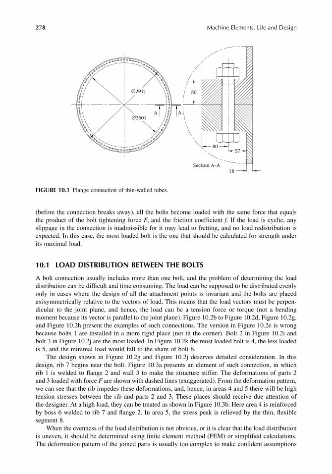
278
Machine Elements: Life and Design
(before the connection breaks away), all the bolts become loaded with the same force that equalsthe product of the bolt tightening force
F
t
and the friction coefficient
f
. If the load is cyclic, anyslippage in the connection is inadmissible for it may lead to fretting, and no load redistribution isexpected. In this case, the most loaded bolt is the one that should be calculated for strength underits maximal load.
10.1 LOAD DISTRIBUTION BETWEEN THE BOLTS
A bolt connection usually includes more than one bolt, and the problem of determining the loaddistribution can be difficult and time consuming. The load can be supposed to be distributed evenlyonly in cases where the design of all the attachment points is invariant and the bolts are placedaxisymmetrically relative to the vectors of load. This means that the load vectors must be perpen-dicular to the joint plane, and hence, the load can be a tension force or torque (not a bendingmoment because its vector is parallel to the joint plane). Figure 10.2b to Figure 10.2d, Figure 10.2g,and Figure 10.2h present the examples of such connections. The version in Figure 10.2e is wrongbecause bolts 1 are installed in a more rigid place (not in the corner). Bolt 2 in Figure 10.2i andbolt 3 in Figure 10.2j are the most loaded. In Figure 10.2k the most loaded bolt is 4, the less loadedis 5, and the minimal load would fall to the share of bolt 6.
The design shown in Figure 10.2g and Figure 10.2j deserves detailed consideration. In thisdesign, rib 7 begins near the bolt. Figure 10.3a presents an element of such connection, in whichrib 1 is welded to flange 2 and wall 3 to make the structure stiffer. The deformations of parts 2and 3 loaded with force
F
are shown with dashed lines (exaggerated). From the deformation pattern,we can see that the rib impedes these deformations, and, hence, in areas 4 and 5 there will be hightension stresses between the rib and parts 2 and 3. These places should receive due attention ofthe designer. At a high load, they can be treated as shown in Figure 10.3b. Here area 4 is reinforcedby boss 6 welded to rib 7 and flange 2. In area 5, the stress peak is relieved by the thin, flexiblesegment 8.
When the evenness of the load distribution is not obvious, or it is clear that the load distributionis uneven, it should be determined using finite element method (FEM) or simplified calculations.The deformation pattern of the joined parts is usually too complex to make confident assumptions
FIGURE 10.1
Flange connection of thin-walled tubes.
A
Section A-A18
80∅2911
∅2601
8057
A
9563_C010.fm Page 278 Monday, July 30, 2007 7:24 PM

Bolted Connections (BCs)
279
about it. Therefore, if we wish to calculate the bolt connection manually, we have to make greatlysimplified assumptions about the deformations of the joint members. Usually, the assumptions areas follows:
• The connected parts don’t deform at all; they are perfectly rigid.• The points of connection are pliable (springy), and all of them (within one connection)
are of the same rigidity.• In connections loaded in tension–compression, the compliance of connection points is
the same in tension and in compression.
FIGURE 10.2
Some cases of even load distribution between bolts.
FIGURE 10.3
A bolt and a rib.
(a) (b) (c) (d) (e)
(f ) (g) (h) (i) (j) (k)
Wrong Wrong Wrong
T
F F
T
F F
1
2 3 45
6
7 7
Wrong
7
F F
(a) (b)
4
5
1
2
3
6
8
7
2
9563_C010.fm Page 279 Monday, July 30, 2007 7:24 PM

280
Machine Elements: Life and Design
In the strictest sense, these assumptions are wide of the truth, but because they are much used, let’sdiscuss them one by one.
When the minimum number of attachment points is used (two in a two-dimensional problemor three in a three-dimensional problem; these problems are called
statically determinate
), thereactions in the attachment points can be determined regardless of the deformations of the bodiesand attachments. But when the number of attachment points is more than minimal (such problemsare called
statically indeterminate
), deformations must be considered to enable calculation ofreaction forces in the attachments.
For statically determinate problems, the rules of engineering mechanics are valid. That means:
• The point of application of a moment to a part is of no significance.• A force applied at any point can be transferred to another point with the addition of an
appropriate moment applied to any point.• A force can be applied to any point coaxially with its vector with no change in the
attachment reactions.
These rules are obviously invalid for statically indeterminate problems. As a case in point, inFigure 10.4 are shown two straight beams loaded with a bending moment
M
. One of them (Figure 10.4a)has two supports, and we can determine the reactions from the following equilibrium equations:
FIGURE 10.4
Examples of statically determinate and indeterminate beams.
RML
R R1 2 1= = −;
M
(a)
L
0.5 L0.5 L
(b)
M
R2
(c)
(d)
R5
R1
R3 R4
x
9563_C010.fm Page 280 Monday, July 30, 2007 7:24 PM

Bolted Connections (BCs)
281
Another beam (Figure 10.4b) is supported in three points and the number of equilibriumequations (two; both the sum of moments and the sum of forces must be zero) is less than thenumber of unknowns (three:
R
3
,
R
4
, and
R
5
). These unknowns can only be determined by applyingvirtual deformations. In this case, if the supports are assumed to be very rigid in comparison withthe rigidity of the beam, we can use the condition that the beam sag at the supports is zero. Forthis purpose, we assume that the middle support doesn’t exist, but instead, force
R
4
is applied inthis point. Then we calculate the deformations as if the beam is statically determinate:
• The sag of the beam in the middle under the action of moment
M
equals
• The sag of the beam in the middle under the action of force
R
4
equals
(Here
E
and
I
are the modulus of elasticity and moment of inertia of the beam.)Because the beam is supported in the middle, the condition of zero sag at this point gives the
following:
Now, when force
R
4
has been determined, we can easily calculate forces
R
3
and
R
5
as in theusual statically determinate problem. And it is obvious from these equations that the forces in thesupports depend on the point of application of the moment (the
x
value).This is not only a formal conclusion based on the equations. Figure 10.4c and Figure 10.4d
show that there is an obvious dependence between the location of moment applied and the defor-mation pattern. This dependence is surely accompanied by corresponding differences in the reactionof supports represented by the preceding equations. When the bending moment is applied in themiddle (as shown in Figure 10.4d),
R
4
=
0, both obviously and mathematically.An example of erroneous application of the rules of engineering mechanics to pliable parts is
presented in Figure 10.5. No doubt, force
F
applied to the bearing’s housing drives it into the
FIGURE 10.5
False use of the parallelogram of forces.
yME I
xL
M = −
12
334
22
yR L
E IR = − 43
48
y y
RM
Lx
L
M R+ =
= −
0
43
344 3
22
(a) (b) (c)
F1 F1
F2 F2
F
9563_C010.fm Page 281 Monday, July 30, 2007 7:24 PM
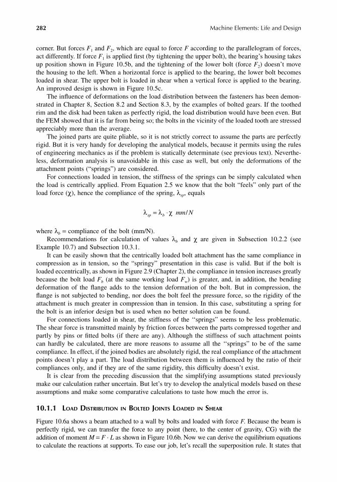
282
Machine Elements: Life and Design
corner. But forces
F
1
and
F
2
, which are equal to force
F
according to the parallelogram of forces,act differently. If force
F
1
is applied first (by tightening the upper bolt), the bearing’s housing takesup position shown in Figure 10.5b, and the tightening of the lower bolt (force
F
2
) doesn’t movethe housing to the left. When a horizontal force is applied to the bearing, the lower bolt becomesloaded in shear. The upper bolt is loaded in shear when a vertical force is applied to the bearing.An improved design is shown in Figure 10.5c.
The influence of deformations on the load distribution between the fasteners has been demon-strated in Chapter 8, Section 8.2 and Section 8.3, by the examples of bolted gears. If the toothedrim and the disk had been taken as perfectly rigid, the load distribution would have been even. Butthe FEM showed that it is far from being so; the bolts in the vicinity of the loaded tooth are stressedappreciably more than the average.
The joined parts are quite pliable, so it is not strictly correct to assume the parts are perfectlyrigid. But it is very handy for developing the analytical models, because it permits using the rulesof engineering mechanics as if the problem is statically determinate (see previous text). Neverthe-less, deformation analysis is unavoidable in this case as well, but only the deformations of theattachment points (“springs”) are considered.
For connections loaded in tension, the stiffness of the springs can be simply calculated whenthe load is centrically applied. From Equation 2.5 we know that the bolt “feels” only part of theload force (
χ
), hence the compliance of the spring,
λ
sp
, equals
where
λ
b
=
compliance of the bolt (mm/N).Recommendations for calculation of values
λ
b
and
χ
are given in Subsection 10.2.2 (seeExample 10.7) and Subsection 10.3.1.
It can be easily shown that the centrically loaded bolt attachment has the same compliance incompression as in tension, so the “springy” presentation in this case is valid. But if the bolt isloaded eccentrically, as shown in Figure 2.9 (Chapter 2), the compliance in tension increases greatlybecause the bolt load
F
b
(at the same working load
F
w
) is greater, and, in addition, the bendingdeformation of the flange adds to the tension deformation of the bolt. But in compression, theflange is not subjected to bending, nor does the bolt feel the pressure force, so the rigidity of theattachment is much greater in compression than in tension. In this case, substituting a spring forthe bolt is an inferior design but is used when no better solution can be found.
For connections loaded in shear, the stiffness of the ‘‘springs” seems to be less problematic.The shear force is transmitted mainly by friction forces between the parts compressed together andpartly by pins or fitted bolts (if there are any). Although the stiffness of such attachment pointscan hardly be calculated, there are more reasons to assume all the ‘‘springs” to be of the samecompliance. In effect, if the joined bodies are absolutely rigid, the real compliance of the attachmentpoints doesn’t play a part. The load distribution between them is influenced by the ratio of theircompliances only, and if they are of the same rigidity, this difficulty doesn’t exist.
It is clear from the preceding discussion that the simplifying assumptions stated previouslymake our calculation rather uncertain. But let’s try to develop the analytical models based on theseassumptions and make some comparative calculations to taste how much the error is.
10.1.1 L
OAD
D
ISTRIBUTION
IN
B
OLTED
J
OINTS
L
OADED
IN
S
HEAR
Figure 10.6a shows a beam attached to a wall by bolts and loaded with force
F
. Because the beam isperfectly rigid, we can transfer the force to any point (here, to the center of gravity, CG) with theaddition of moment
M
=
F
·
L
as shown in Figure 10.6b. Now we can derive the equilibrium equationsto calculate the reactions at supports. To ease our job, let’s recall the superposition rule. It states that
λ λ χsp b mm N= ⋅ /
9563_C010.fm Page 282 Monday, July 30, 2007 7:24 PM

Bolted Connections (BCs)
283
the summary effect of forces on a system equals the sum of effects of each force of the system. So wecan consider separately the reactions at supports caused by
F
and
M
and then sum up the results.Force
F
causes linear motion of the beam relative to the wall. (As you would remember, thereis a direct proportionality between the relative motion and the stress.) Because the wall and thebeam are absolutely rigid, all the points of attachment become deformed by the same amount.Inasmuch as all the attachments are of the same compliance, their reactions should be equal. Hence,the load of bolt
i
caused by force
F
equals
(10.1)
where
n
=
the number of bolts in the connection.Moment
M
turns the beam relative to the wall around the CG point, and the relative movementin each attachment is directly proportional to its distance from CG; hence, the load of bolt
i
causedby moment
M
is directly proportional to radius
r
i
(see Figure 10.6b). Now we can write the followingequations:
(10.2)
FIGURE 10.6
Bolt connection loaded in shear.
F
M
(a)
L
F
Center of gravity (CG)
(b)
(c)
rmaxri
RFnF i, =
R
R
r
r
R Rr
r
M i
M
i
M i Mi
,
,max max
, ,maxmax
=
=
9563_C010.fm Page 283 Monday, July 30, 2007 7:24 PM

284
Machine Elements: Life and Design
where
R
M,
max
=
reaction of bolt with the maximal radius
r
max
r
i
=
distance between bolt number i and the CG point
r
max
=
maximal distance between bolt and the CG point
The equilibrium equation for this case looks as follows:
(10.3)
Insertion of Equation 10.2 into Equation 10.3 gives us the maximal load caused by moment
M
:
(10.4)
As soon as we know the
R
M
,max
value, we can calculate the
R
M,i
for each bolt using Equation 10.2,and then the summary load of each bolt can be determined.
If the bolts are equally spaced on a circle as shown in Figure 10.6c, then the former equationschange as follows:
Forces
R
F,i
are directed like force
F
, but forces
R
M,i
are directed tangentially, that is, perpendicularto the line connecting the bolt
i
with CG. This means that each bolt has a different direction offorce
RM,i, and its sum with RF,i should be vectorial.You can ask, “Why on earth did you decide that the center of rotation (CR) is the CG point?
In fact, we can select any other point as CR, so that the Σri2 value in Equation 10.4 be greater and
the force RM,max, lesser.” Unfortunately, the only way to place CR according to our wish is to makea real axle with bearings. In our case, there is no such thing, and the parts choose CR so as tominimize the resistance of the bolt joint to the rotation, i.e., to make the Σri
2 value minimal. Thereis rigorous proof that this point is placed exactly at the CG of the connection, but we want todemonstrate this by a simple example. Figure 10.7 presents a two-bolt connection subjected totorque. The CG point here is placed in the middle of the distance between them, so that r1 = r2 = r,and Σri
2 = 2r2. It is clear that if we transfer the CR horizontally (to the right or to the left), bothr1 and r2 grow. What if we transfer the CR vertically by some amount ∆, to point O? In this casethe Σri
2 value increases as well:
The same can be shown for any quantity of bolts. Here, we can see that any drift of CR from CGleads to increase in the Σri
2 value. Therefore, CR displaced from CG can’t be chosen by the partsvoluntarily, without some real constraint such as a spigot or an axle.
Let’s make several comparative calculations.
M R rM i i= ⋅Σ ,
MR
rr
RM r
r
Mi
Mi
=
= ⋅
,max
max
,maxmax
Σ
Σ
2
2
r r r
r n r
RM
n r
i
i
M
max = =
= ⋅
=⋅
Σ 2 2
Σ ∆ ∆ ∆r r r ri2 2 2 2 22 2= + + − = +( ) ( )
9563_C010.fm Page 284 Monday, July 30, 2007 7:24 PM

Bolted Connections (BCs) 285
EXAMPLE 10.2 (FIGURE 10.8A)
Beam 1 is attached to wall 2 by 12 bolts and loaded with force F = 10,000 N. The load must betransmitted by friction forces. Dimensions are given in the sketch.
Moment of force F around the CG point: M = 10,000 · 1,000 = 10 · 106 N·mm. There are fourbolts with r = rmax = 201 mm, two bolts with r = 180 mm, four bolts with r = 108 mm and twobolts with r = 60 mm. Thus,
From Equation 10.4, the maximal bolt load from moment M equals
The bolt load from force F equals
Among the 12 bolts numbers 3, 4, and 5 are obviously the most loaded for they are far from CRand both the RM and RF forces act in nearly the same direction. Bolts 3 and 5 are loaded equally:
FIGURE 10.7 The center of gravity (CG) and the center of rotation (CR).
CG
∆
CR
r1
r2
Σr mmi2 2 2 2 2 5 24 201 2 180 4 108 2 60 2 8 10= ⋅ + ⋅ + ⋅ + ⋅ = ⋅.
R NM ,max .= ⋅ ⋅
⋅=10 10 201
2 8 107180
6
5
R NF = =1000012
833
9563_C010.fm Page 285 Monday, July 30, 2007 7:24 PM

286 Machine Elements: Life and Design
vectorial sum of RM,max and RF equals R3 = R5 = 7930 N (see the geometric summation in Figure 10.8b).Bolt 4 is loaded by forces RM,4 and RF acting in the same direction, so these two forces can be justsummed. From Equation 10.2,
Thus, the load of bolt 4 equals
Finally, according to this calculation the most loaded bolts are 3 and 5, and R3 = R5 = 7930 N.Calculation made using FEM gives R3 = R5 = 9450 N (the force vectors with their values are
shown in Figure 10.8a), but the maximal bolt load R6 = R7 = 11250 N, that is, 1.42 times greaterthan was obtained under the assumption that beam 1 and wall 2 are absolutely rigid.
EXAMPLE 10.3 (FIGURE 10.9)
Part 1 loaded with force F is attached to part 2 by 12 bolts. Force F passes through the CG of theconnection. So if the parts are absolutely rigid, all the bolts (see Figure 10.9a and Figure 10.9b)are loaded evenly, and the load equals
If F = 10,000 N, R = 833 N. But calculations using FEM show that the load distribution is uneven.The vectors of bolt forces and their magnitudes (in Newtons) are shown with arrows in Figure 10.9.
FIGURE 10.8 Sketch to Example 10.2.
CG
F
1
2
543
1000
RM,max
RFR3
3CG
r max
(a)
(b)
6
11250
7
5450 4560
9450
11250 5450 45609450
3960
1770503
5670
4
180180
201
120 120
60 90
90
120
2020
R NM ,4 7180180201
6430= =
R R R NM F4 4 6430 833 7263= + = + =,
RF=12
9563_C010.fm Page 286 Monday, July 30, 2007 7:24 PM

Bolted Connections (BCs) 287
We can see that in Figure 10.9a the maximal bolt load is 2,100 N, which is 2.5 times greater thanthe average amount of 833 N. In Figure 10.9b, the maximal bolt force (1370 N) is 1.64 timesgreater than the average.
How should we regard these results? The simplified calculations are very approximate, but thisis better than nothing. In less important cases, the designer, in order to account for the possibledifference between the calculated and real load of the bolt, just increases the safety factor andkeeps in mind that after the friction forces fail to transmit the load, the shanks of bolts go intoaction and work as pins. In more important cases, the designer uses elements loaded in shear (suchas fitted bolts, pins, or keys) in addition to the friction forces. In this case, the calculation is usuallymade separately for the friction forces and for the shear elements, as if each of them had to transferthe entire load with a certain factor of safety. In very important cases, special research is usuallyarranged, including FEM calculations and laboratory tests for strength. That is not an easy task.
10.1.2 LOAD DISTRIBUTION IN BOLTED JOINTS LOADED IN TENSION
Figure 10.10a presents a model, in which 1 and 2 are the connected parts and 3, the springs replacingbolts. In the unloaded position, all the springs are assumed to be unloaded. As mentioned, thepresentation of the joined bodies as perfectly rigid means that all the forces can be transferred tothe CG of the connection (with the addition of appropriate moments). It is obvious that force Fapplied in the center of the connection causes all the springs to be deformed (and loaded) equally,as shown in Figure 10.10b. Moment M applied to the rigid body causes the body to turn aroundthe axis that passes through the CG of the connection and is collinear with the vector of the moment,as shown in Figure 10.10c. The deformation of each spring is directly proportional to the distanceof this spring from the turning axis.
The reason for the turning axis to pass through the CG point is exactly the same as for theconnections loaded in shear: this placement of the axis meets the minimal resistance of theconnection to turn. Moment M is placed here in the center of connection just for the pleasureto see all the loads applied in one point. But inasmuch as the body is considered absolutelyrigid, the moment can be applied at any point of the body with no influence on the springdeformation pattern.
FIGURE 10.9 Sketch to Example 10.3.
F1
2
2020
F
(b)(a)
2100 1150530 190
1310 1340 800280
1640 1170100
840
2060
9701370 1370
970 90
90540
960 960
100
540
370
1030 1030
370
120 120 120
90
90
120 120 120
9563_C010.fm Page 287 Monday, July 30, 2007 7:24 PM

288 Machine Elements: Life and Design
Figure 10.11 shows a scheme of a bolt connection that has two axes of symmetry. After all theforces are repositioned to the CG of the joint, we have one force F (perpendicular to the jointsurface) applied in the center, and two moments Mx and My.
There can also be forces and moments that load the connection in shear, but they should beconsidered separately as shown earlier.
To derive the equilibrium equations, we consider separately the reactions at supports causedby F, Mx, and My and then sum up the results. We begin with F. As already mentioned, the tension(or pressure) force applied at the CG is distributed evenly between the bolts. Thus, bolt i is loadedby a force
(10.5)
where n = number of bolts.
FIGURE 10.10 Elements of the analytical model for bolt joint loaded in tension and bending.
FIGURE 10.11 Schematization of bolt connection loaded in tension and bending.
F
M
Unloaded
2
3
1
(a) (b)
(c)
RFnF i, =
X
Y
X
YX
max
Ymax
Xi
Yi
My
Mx
FCG
9563_C010.fm Page 288 Monday, July 30, 2007 7:24 PM

Bolted Connections (BCs) 289
The next step is to determine the reactions from the moments. Moment Mx is balanced by thetotal moment of the forces of bolts. Partial moment mi,x about axis X applied by bolt i equals
(10.6)
where Rix = reaction of bolt i caused by moment Mx.(As said earlier, the bolt reaction is directly proportional to the distance from the axis, in this
case, to the coordinate y.)Now we can write the following:
(10.7)
where Rmax,x = reaction of the bolt with the maximal distance (ymax) from axis X.Insertion of Equation 10.7 into Equation 10.6 gives
(10.8)
In the same way, we can calculate the maximal bolt reaction caused by moment My:
(10.9)
In the case under consideration, the maximal reactions Rmax,x and Rmax,y are related to the samebolt, and the total maximal reaction equals the sum of three components presented by Equation 10.5,Equation 10.8, and Equation 10.9:
(10.10)
The joint shown in Figure 10.11 is very handy for calculation. It is not always so. For example,in a round connection shown in Figure 10.12a, bolts 1 and 3 have the maximal reaction frommoment Mx, but zero reaction from moment My. Conversely, bolts 2 and 4 have their maximalreaction from moment My and zero reaction from moment Mx. Therefore, in this case, the reactionof each bolt should be calculated using Equation 10.7 and Equation 10.8 for Mx and likewise forMy, and then the maximal reaction can be obtained as the maximal value of their sum.
For joints that have only one symmetry axis (Figure 10.12b), the location of the neutral axis(X in this case) should be determined for the condition Σyi = 0.
m R yi x i x i, ,= ⋅
R
R
y
y
R Ry
y
i x
x
i
i x xi
,
max, max
, max,max
=
=
m Ry
yM m
R
yy
R
i x xi
x i xx
i, max,max
,max,
max
;= = =2
2Σ Σ
mmax,max
xx
i
M y
y=
Σ 2
RM x
xyy
imax,
max .=Σ 2
RFn
M y
y
M x
xx
i
y
imax
max max= + +Σ Σ2 2
9563_C010.fm Page 289 Monday, July 30, 2007 7:24 PM

290 Machine Elements: Life and Design
If the joint has no symmetry axes, the CG location can be found in the following way:
Put the X and Y axes in any position with respect to the joint; don’t forget that these axesshould be perpendicular to each other.
Calculate the proper position of these axes using the condition Σxi = 0 and Σyi = 0; theintersection of these axes is the required CG point.
Take the projections of the load vectors onto the X–Y axes (you can rotate these axes aroundthe CG for the sake of convenience) and calculate the reactions of each bolt using Equation10.7 to Equation 10.10.
EXAMPLE 10.4
Figure 10.13 shows a housing attached to a rigid foundation by 10 bolts numbered from 1 to 10.Vertical force F = 1000 N has been applied to the housing upward in different points numberedfrom 11 to 20. In each load case, the bolt reactions have been calculated twice: using Equation 10.7to Equation 10.10 and also by FEM.
For this connection, the following data are invariant for all ten loading options:
To make calculations using Equation 10.10, force F is transferred from the point ofapplication to the CG, and the associated moments Mx and My are given in Table 10.1. Themaximal bolt reactions Rmax are given in Table 10.2. In the same table are summarized themaximal bolt reactions found using FEM. By this method, the following versions of theconnection have been calculated:
FIGURE 10.12 Bolt connection contours of greater complexity.
X
Y1
2
3
4
Y
X
(a) (b)
yi
x mm y mm n
xi
max max; ;
.
= = =
= ⋅ =
150 450 10
10 150 2 252 2Σ ⋅⋅
= ⋅ + ⋅ = ⋅
10
4 450 4 225 10 125 10
5 2
2 2 2 5 2
mm
y mm
x
i .
max
ΣΣ Σxmm
y
yi i2 5
4 12
1502 25 10
6 67 1045=
⋅= ⋅ =− −
.. ; max 00
10 125 104 44 10
54 1
..
⋅= ⋅ − −mm
9563_C010.fm Page 290 Monday, July 30, 2007 7:24 PM

Bolted Connections (BCs) 291
• The steel housing is solid, and the compliance of the attachment point λsp = 1.79 · 10−7 mm/N(these reactions are labeled R1max).
• The steel housing is hollow, wall thickness equals 12 mm, and λsp = 1.79 · 10−7 mm/N(R2max).
• The housing is solid, and λsp = 10.2 · 10−7 mm/N (R3max).• The housing is hollow, wall thickness equals 12 mm, and λsp = 10.2 · 10−7 mm/N (R4max).
In Table 10.2, we see that there is a certain difference in bolt reactions obtained from Equation 10.10and FEM, but this difference is not too large and in the worst case it reaches 60%. So if we takesome spare safety factor, say, 1.5 or 2, we can countervail the possible error of the simplifiedcalculation. But if the higher safety factor is not affordable, the bolt stresses should be calculated
FIGURE 10.13 Sketch to Example 10.4.
TABLE 10.1Bending Moments in the Bolt Connection
Point of Load Application Mx, kNmm My, kNmm
11 0 012 225 013 450 014 0 15015 225 15016 450 15017 0 15018 225 15019 450 15020 450 0
Note: See Example 10.4.
X
Y
My
Mx
F
600
900
300
1
2
3
4
5
10
9
8
7
6
11
12
1316
15
14
20
19
18
17
9563_C010.fm Page 291 Monday, July 30, 2007 7:24 PM

292 Machine Elements: Life and Design
more accurately and checked by direct measurements, because any calculation involves simplifi-cations in the definition of boundary conditions.
10.2 TIGHTENING OF BOLTS
10.2.1 TIGHTENING ACCURACY
The needed pressure in a BC is achieved by tightening the bolts. The stronger the tightening, thestronger is the connection. Modern fasteners allow high tightening forces. For example, bolt M12of property class 10.9 can be tightened by a force of 55,000 N, and bolt M24 by 230,000 N. Ifthere are several such bolts in the connection, the connected parts may be pressed against eachother by a force of hundreds of tons, provided that the bolts are tightened properly.
Until the middle of the 20th century, tightening torque was not usually specified in drawings:it was common practice to rely on a qualified fitter, except for important and highly loaded boltedconnections. In the course of time, industrial production became multifarious, with machines beingquickly replaced by new models that bear relentlessly increasing loads, and it has become necessarythat fitters should get to know the tightening torques for each connection from the technicaldocumentation. Therefore, the specification of this parameter is nowadays a general practice.
EXAMPLE 10.5
Once during the shop test of a marine engine, a failure occurred in the intermediate shaft thatwas transmitting power of 6000 HP at 250 r/min from the engine to a hydraulic brake. Shaft 1(Figure 10.14), 250 mm in diameter, broke because of fatigue crack 2 that originated from a holefor cone bolt 3. Investigation of this case revealed that there was fretting damage in all these holes,and in all fretted areas, there were initial fatigue cracks. But what was the cause for the frettingdamages and cracks?
That flange connection had been calculated for strength during design, and when the shaftfailed, there was no problem ascertaining the cause of this event. In the assembly drawing therewas not specified tightening torque for the bolts that are M42 in diameter. The fitters (by the way,very qualified fitters occupied with assembly of diesel engines) tightened the bolts as strongly aspossible without the use of any special devices. But the friction force between the flanges ofshaft 1 and resilient coupling 4 was inadequate to withstand the shear force in this connection.
TABLE 10.2Comparative Calculations of Bolt Connections
Point of Load Application Rmax, N R1max, N R2max, N R3max, N R4max, N
11 100 123 119 120 12712 200 197 196 177 18813 300 274 327 266 32114 200 263 268 234 26815 300 328 305 292 30516 400 409 421 357 42217 200 270 319 237 27518 300 334 347 295 30919 400 410 475 357 45020 300 277 336 268 323
Note: See Example 10.4.
9563_C010.fm Page 292 Monday, July 30, 2007 7:24 PM
Bolted Connections (BCs) 293
In operation, the cone bolts transmitted most of the shear force with some micromovements causedby load fluctuations and torsional vibrations. These micromovements caused fretting damages, andthe resulting origination of fatigue cracks was inevitable.
The designer rectified the error and specified the tightening torque: 6000 N·m. The failed shaftwas replaced by a new one. The coupling was renewed by machining the cone holes together withthe new shaft to increased diameters (to take away the fretted layer and to make sure that therewere no fatigue cracks left). The cone-fitted bolts were replaced as well. The fitters built a hugelever and tightened all the bolts with the needed torque. This defect never occurred again.
How did the designer (in Example 10.5) calculate the tightening torque? First, he calculatedthe tightening force Ft needed to transmit the shear force (see Subsection 10.3.2). Then, he chosethe quantity and diameter of bolts. And then, as he had established the diameter of thread and thetightening force, he obtained the tightening torque from this equation:2
(10.11)
Here,Ft = tightening force (N)d = thread diameter (mm)p = thread pitch (mm)RN = mean radius of the nut (or bolt head) bearing surface (mm)µT and µN = coefficients of friction in the thread and on the bearing surface of the nut (or bolt
head), respectively
In fact, µT > µN because the unit pressure in the thread is higher, the oil film is thinner, and theshare of metal-to-metal contact is bigger. Besides, the sliding couples may be different: the nutand the bolt are usually made of steel, and the connected parts are often made of gray cast iron,aluminum, or copper alloys that are characterized by a lower coefficient of friction. But in practicethere is usually no possibility to separate these two tribological situations. Provided that µT = µN,Equation 10.11 can be converted into a simple dependence between the tightening torque Tt and
FIGURE 10.14 Flange connection with cone-fitted bolts.
14
3
2
5
A
A
Section A-A
The cone bolt is
extracted
T Fd p
dRt t T N N= +
+
21 15
πµ µ.
9563_C010.fm Page 293 Monday, July 30, 2007 7:24 PM

294 Machine Elements: Life and Design
the tightening force Ft. For some standard ratio of dimensions (for example, RN ≈ 0.7d and p ≈ 0.125d),it is the following:
(10.12)
where kt = 0.15, 0.18 and, 0.20 for µT = µN = µ = 0.1, 0.125, and 0.140, respectively.In experiments with bolts M12 × 1.5, the following coefficients of friction were obtained:2
With no lubrication:• Uncoated threads — µ = 0.12–0.25 (sometimes 0.55 because of seizure)• Cadmium-plated threads — µ = 0.18–0.32• Copper-plated threads — µ = 0.13–0.32
Lubricated with machine oil:• Uncoated threads — µ = 0.10–0.17• Cadmium-plated threads — µ = 0.14–0.18• Copper-plated threads — µ = 0.12–0.19
In different experiments, the µ value may differ, but the following conclusions can be drawn:
1. Before tightening, the threads should be greased or oiled, because that prevents seizure,decreases the dispersion of the µ value, and improves the tightening accuracy.
2. Considering the dispersion of the friction coefficient, the tightening torque value can becalculated with an accuracy of ±(20–25)%.
For critically loaded BCs, such error is not acceptable, and then the tightening force should becontrolled by methods that leave the friction forces out. The most exact method consists inmeasuring the bolt elongation. In this case, the friction forces don’t influence the tightening forcedetermination, though they do influence the bolt stress through its torsion.
For tightening large bolts, hydraulic devices are used. The hydraulic piston is connected to thethread (which is made longer to project from the nut) and applies force Ft to the bolt. Then the nutis tightened manually by a wrench, which applies to the bolt some additional force that is negligiblein comparison with Ft. This method is exactly similar to the previous one, but the bolt shank is nottorsioned. This means that the stress in the bolt is less by about 1.3 times, and the tightening forceFt can be increased correspondingly.
Both of these methods are laborious and used only sometimes, when the exact and reliabletightening of bolts is a must. As cases in point, the connecting rod bolts and cylinder head studsof high-power diesel engines can be mentioned.
One more method of tightening, less exact but not influenced by friction, consists in turningthe nut (or the head of bolt) by a specified angle. This is aptly called the “turn-of-the-nut” method.The tightening is executed in two steps: first, the nut should be tightened by a relatively small forceto take up clearances, and then it should be turned by a certain additional angle. The deformationswhile tightening include not only elongation of the bolts, but also contraction of the connectedparts, plastic deformation and wear of the roughness (called embedment), and plastic deformationsin the thread. Most of these factors can hardly be calculated with acceptable accuracy. Therefore,the preliminary tightening torque and the angle of additional turn should be determined experi-mentally on prototype models, when the real tightening force Ft can be controlled by strain gaugesor by measuring bolt elongation. This method can be recommended for long bolts (more than sixdiameters in length). With shorter bolts, the accuracy of this method is too low because the angleof rotation of the nut is rather small.
If the bolted connection is designed with a generous safety factor, a torque wrench is used totighten the bolts. This method is the easiest. The nominal tightening torque can be obtained from
T k F dt t t=
9563_C010.fm Page 294 Monday, July 30, 2007 7:24 PM

Bolted Connections (BCs) 295
Equation 10.11 or Equation 10.12, in which the values of Ft and the coefficients of friction shouldbe preselected. Because the real coefficient of friction can be less than the chosen one, force Ft
developed by the nominal tightening torque may be larger than planned, and the bolt may beoverstressed. To prevent this possibility, the nominal torque should be decreased by about 20–25%.But the coefficient of friction may be also bigger than the preset one by 20–25%, and in this case,the real tightening force (taking into account the decreased tightening torque) may come to 65–56%of the preset value. That is the payment for the inexact method of tightening.
10.2.2 STABILITY OF TIGHTENING
Proper tightening of bolts is necessary but insufficient to have a reliable connection: the tighteningforces may decrease in course of time, and the tightening may remain proper only on the drawing.What can be the cause of this torque retention loss? There are several such factors, as describedin Subsection 10.2.2.1 and Subsection 10.2.2.2.
10.2.2.1 Self-Loosening of Bolts
All bolt threads are self-braking, or, in other words, the lead angle of the thread is less thanthe angle of friction. That means, if you have tightened the thread and began staring at itattentively, you are just wasting your time: it will not unscrew, even if you wait very long andwatch with unrelenting interest. It will unscrew later, when the machine works. But why? Willsomething have changed? Yes, sure! Under the influence of vibrations and micromovements,including the variable radial deformation of the nut under variable bolt load (the nut is “breath-ing”), the coefficient of friction decreases. How much? It depends on the amplitude andfrequency of vibrations. If, usually, µ = 0.10–0.15, under vibrations it changes cyclically (inaccordance with the local microslip in the contact places), and the lowest value during a cyclemay be as low as 0.01 or even 0.005. During these very small periods of time, the thread ceasesto be self-braking, and the fasteners begin to unscrew little by little, if they have not been locked(see Subsection 10.2.3).
10.2.2.2 Plastic Deformation of Fasteners and Connected Parts
It can be related to the following factors:
Creep of metal: Creep, i.e., slow plastic deformation of a metal under load, exists alwaysto a greater or lesser extent. But at higher temperatures, it increases by far. The temperatureswhen creep should be considered a possibility are 300°C for construction steels and150°C for light alloys. Above these temperatures, high-temperature materials must beused.
It should be noticed that the harmful influence of high temperature manifests itself notonly in the creep of materials. In the literature, one can find information that at a temperatureabove 200°C the parts should not be plated with zinc, cadmium, tin, and bismuth, becausethese materials diffuse into the surface layer of the part (Rebinder’s effect) and impair itsstrength. At higher temperatures copper and brass coatings that have considerably highermelting points are acceptable.
Occasional overload that causes plastic deformations of the connection members: It isusually cheaper to replace the fasteners that have slackened because of overload than itis to examine them and incur risks using them again. The connected parts may need someadditional machining, if their joint surfaces have been damaged when working withslackened fasteners.
Surface plastic deformation of the connected parts underneath the nut or head of bolt: Thebearing surface of the nut (head of bolt) nearly equals the cross section of the thread.
9563_C010.fm Page 295 Monday, July 30, 2007 7:24 PM

296 Machine Elements: Life and Design
Both of them are exposed to the same bolt force Fb; therefore, the yield points of thematerials should be comparable. Tab washers and locking plates made of mild steel arenot suitable for high-strength fasteners (property class 8.8 and higher). If a high-strengthbolt is tightened against a tab washer, the latter creeps out from under the nut as if it wasmade of plastic.
It is clear that the admissible bearing stress should not be exceeded. When the connectedparts are made of softer materials (for example, aluminum or magnesium alloys), specialmeasures should be taken to increase bearing surfaces. Figure 10.15a shows a bolt andnut made of high-strength stainless steel and designed for light metal parts. The bearingsurfaces of the nut and the bolt head have been developed so as to decrease the surfacepressure to a permissible value.
Figure 10.15b shows a connection with standard fasteners and thick steel washers 1and 2 that are intended to distribute the bolt force over a bigger surface. The thickness ofthe washers depends on the bearing surface to be achieved on the softer material.
Figure 10.16a presents isobars in a tightened BC. It is clear that outside diameter d2
washer 1 is separated from the flange, and increasing the washer beyond diameter d2 isuseless. Because the isobars in this area are inclined at about 45°, the effective diameterof the washer can be determined as follows (see Example 10.6):
whered1 = diameter of the bearing surface of the nut (or head of bolt)h = thickness of the washer
Plastic deformation of micro-asperities: The initial plastic deformation happens duringtightening. Later, the microasperities continue flattening under the influence of high pres-sure and micromovements between the surfaces. As a result, the fasteners lose part of theirtightening force. Plastic deformation is especially significant for short bolts of low propertyclass, because their tightening elongation is relatively small.
FIGURE 10.15 Bolt connection of aluminum parts.
d d h2 1 2= +
(a) (b)
1
2
9563_C010.fm Page 296 Monday, July 30, 2007 7:24 PM

Bolted Connections (BCs) 297
EXAMPLE 10.6
Bolts M20–8.8 connect flanges made of aluminum alloy with tensile strength of 200 MPa. The permis-sible surface pressure for this material p = 140 MPa.6 Tightening force for this bolt Ft = 113,500 N;hence, the bearing surface should equal
The diameter of the hole equals 22 mm; its surface is 380 mm2, so the area inside diameter d2
should be 811 + 380 = 1191 mm2. Hence, the effective diameter of the washer
The minimal diameter of the bolt head bearing surface d1 = 28.2 mm. Hence, the needed thicknessof the washer
If the bolt was of property class 10.9, the tightening force would be 159,000 N, the neededdiameter of the washer d2 = 44 mm, and its minimal thickness h = 7.9 mm.
EXAMPLE 10.7
Bolt M20–4.8 tightens two steel flanges 20 mm thick each (Figure 10.17a). Under the nut and bolthead there are installed tab washers each 1.6 mm thick. The tightening force Ft = 50,000 N. Let’sfirst calculate the elastic deformations of the connection members using Birger’s recommendations.2
FIGURE 10.16 Stress distribution in tightened bolt connection.
1
2h
d2
d1
(a) (b)
d0
α
AF
pmmt= = =113500
140811 2
dA
mm2
4 4 119139= = ⋅ =
π π
hd d
mm= − = − =2 1
239 28 2
25 4
..
9563_C010.fm Page 297 Monday, July 30, 2007 7:24 PM

298 Machine Elements: Life and Design
1. Compliance of the bolt. This includes the following:• Compliance of the thread:
whereE = modulus of elasticity (MPa)d = diameter of thread (mm)
• Compliance of the bolt head:
where h = height of the bolt head (mm).• Compliance of the bolt shank:
Here, L = length of shank between the bearing surfaces of the nut and the bolt head (mm)AS = cross-sectional area of the shank (mm2)
The total compliance of the bolt equals
FIGURE 10.17 Comparison of bolt designs.
(a) (b) (c) (d)
1
1.6
20
20
L
λt d Emm N≈ =
⋅ ⋅= ⋅ −0 85 0 85
20 2 06 102 06 10
57
. ..
. /
λh h Emm N≈ =
⋅ ⋅= ⋅ −0 15 0 15
12 5 2 06 100 58 10
57
. .. .
. /
λshS
LE A
mm N= =⋅ ⋅
= ⋅ −43 22 06 10 314
6 68 105
7.
.. /
λ λ λ λb t h sh= + + = + + = ⋅− −( . . . ) .2 06 0 58 6 68 10 9 32 107 7 mmm N/
9563_C010.fm Page 298 Monday, July 30, 2007 7:24 PM

Bolted Connections (BCs) 299
The elastic elongation of the bolt under tightening force equals
2. The compliance of the flanges can be obtained from the following equation:2
(10.13)
Dimensions d1, d0 and angle α are illustrated in Figure 10.16. Angle α determines the so-called‘‘cone of pressure” (hatched). There are shown also isobars, and lines 2 are the zero isobars (insidethe line the stress is compressive and outside, tensile). This means that the “cone of pressure” hasno physical meaning: it is just an artifice used to calculate the compliance of the connected parts.The recommended angle of the cone is α ≈ 22–27°. The error of this calculation usually lieswithin admissible limits. Because the value of λf directly influences the bolt force under load (seeChapter 2, Subsection 2.3.1), in important cases, it should be estimated more exactly by FEM orexperimentally.
In our case, d1 = 28.2 mm, d0 = 22 mm, L = 43.2 mm, tan α = 0.5, and E = 2.06 · 105 MPa.From Equation 10.13, λf = 3.2 · 10−7 mm/N. Now the elastic deformation of the flanges can becalculated:
So the total elastic deformation of all connection members equals 0.047 + 0.016 = 0.063 mm.There are six pairs of contacting surfaces in this connection. If the mean height of microas-
perities equals 5 µm, and if in course of time they plastically deform by one third of theirheight, the elastic deformation of the connection members will decrease by 20 µm (that is 32%of the initial deformation of 63 µm), and the prestress force will decrease from 50,000 N to34,100 N.
For the same purpose we can use bolt M12–10.9 with tightening force Ft = 54,000 N(Figure 10.17b). Using the same formulas and taking into account that there are no tab washers,the following values of compliances have been found:
The summary elastic deformation in this case equals 0.124 + 0.031 = 0.155 mm. In addition, thereare only four pairs of contacting surfaces, so the same plastic deformation of microasperities leadsto only 13 µm of tightening loss. This comprises 8.4% of the initial tightening, and the prestressdecreases from 54,000 N to 49,470 N.
If the bolt is made with a shank decreased in diameter to 90% of the outer diameter of thethread (Figure 10.17c), the loss of elastic deformation will be only 6.9%. Thus, all the abovemeasures — using higher grade bolts, lessening the roughness of the contacting surfaces, anddecreasing the quantity of connected parts — contribute to the stability of the joint.
∆b t bF mm= = ⋅ ⋅ =−λ 50000 9 32 10 0 0477. .
λπ α
αf
fE d
d d d L d
d d= + + −
−2
0
1 0 1 0
1 0tanln
( )( tan )( )(dd L d1 0+ +tan )α
∆ f mm= ⋅ ⋅ =−50000 3 2 10 0 0167. .
λ λ λt h smm N mm N= ⋅ = ⋅ = ⋅− −3 44 10 0 97 10 18 567 7. / ; . / ; . 110
22 97 10 54000 22 97 1
7
7
−
−= ⋅ = ⋅ ⋅
mm N
mm Nb b
/
. / ; .λ ∆ 00 0 124
5 73 10 54000 5 73
7
7
−
−
=
= ⋅ = ⋅ ⋅
.
. / ; .
mm
mm Nf fλ ∆ 110 0 0317− = . mm
9563_C010.fm Page 299 Monday, July 30, 2007 7:24 PM

300 Machine Elements: Life and Design
10.2.3 LOCKING OF FASTENERS
It is not always known beforehand whether a connection needs locking or not. Therefore, thedesigner usually locks the fasteners using some cheap and easily available means just to feel morecomfortable. The trials of the prototype may reveal insufficiency or redundancy of the lockingmethod used.
Methods of locking fasteners are abundant, but they may be classified into two groups. In thefirst group, the nut is locked directly against the shank of the bolt. Among these methods, the mostwidespread are castle nut with a split pin (known as a cotter pin), self-locking nut and jam nut. Inthe second group, both the nut and the bolt are locked separately against the connected parts. Thatgroup encompasses spring lock washers, serrated lock washers, plastically deformable tab washers,nuts with a conical bearing surface, wiring, and other methods.
Each of these locking methods has its merits and weaknesses. For example, split pins(Figure 10.18a) are reliable, but they influence the tightening of the bolt: to align the holes in thebolt shank and the slots in the castle nut, the bolt will usually be a bit overtightened or undertight-ened. Therefore, it is unacceptable for short bolts. Besides, if the material of the pin is not softenough, the bent area may become cracked, and in service, the bent up end may fall off, get betweenmoving parts and damage the mechanism.
The idea of self-locking nuts is to increase the friction in the thread by a certain amount, whichis independent of the tightening force and less liable to be influenced by vibrations. For this purpose,unthreaded plastic inserts have been integrated into the nut (Figure 10.18b; the bolt “threads” theplastic when screwing up). In another type, the thread of the nut is deformed in some small area,so that the bolt enters this area with interference. Both the plastic insert and the deformed threadsare made in the less loaded end of the nut, which is opposite to the bearing surface. Therefore,they don’t impair the load capacity of the bolt and are much less influenced by vibrations. Bothof the aforementioned nut types are commonly classified as prevailing torque.
Self-locking nuts with a plastic insert are sensitive to increased temperature: their limit is about80–100°C. This means that hot oil or even long exposure to the sun in a hot climate may damagethe insert. Self-locking nuts with deformed thread are more reliable and can be used several times.
Using of jam nuts (Figure 10.18c) is the most questionable and old-fashioned way of locking.Nowadays it is considered unreliable. Besides, when the jam nut is tightened, it takes part of thebolt force or, possibly, the whole force. This uncertainty may lead to a failure, because the jam nut
FIGURE 10.18 Locking fasteners.
ka
3
1
4
5
c
d
b
e
f g h
i
j
l
m
n
6
2
9563_C010.fm Page 300 Monday, July 30, 2007 7:24 PM

Bolted Connections (BCs) 301
is not strong enough. Also, this uncertainty may lead to loosening of the bolt, because two nuts,one of which is not loaded, are the same as a single nut.
The spring lock washer (Figure 10.18d) is, in essence, a single coil of a spring with rectangularcross section. Its slit is provided with sharp edges that project from the bearing surfaces. Under load,they indent by a small amount the bearing surfaces of both the nut and the flange. The direction ofthe slit is chosen so that when tightening, the sharp edges just slip, but when unscrewing, they worklike chisels trying to chip the surfaces. The force needed to chip creates the locking effect. If thesurfaces the spring washer contacts are too hard (more than 300 HB), the sharp edges can’t do theirwork as needed, and the locking effect decreases. But when the material is soft (say, less than 150 HB),the slit really cuts the surfaces. Therefore, a flat washer should be placed between the spring lockwasher and the soft flange (for example, one made of aluminum or magnesium alloys). In that case,the locking effect is caused only by the spring force of the washer, and it is quite low.
The projecting sharp edges of the slit cause uneven load distribution around the bearing surfaceof the nut (or the bolt head). This may be an important drawback for critically loaded bolts because itadds bending moment to the bolt shank. From this point of view, serrated lock washers (Figure 10.18e)are preferable; they are provided with many “chisels” distributed evenly around the circle. The advisablehardness of the surfaces contacting the serrated washer lies between 250 HB and 300 HB.
Tab washers (Figure 10.18f) lock the nut (or the head of bolt) in any position. The tab washershould be bent in position 1 or 2, but the nut (bolt), when tightened, often turns the washer toposition 3. The fitter will then have to turn it back to position 1, but the bolt has been alreadytightened, and the fitter may be careless enough to leave the washer in position 3 when bending itto contact the nut. This washer doesn’t lock because the nut can unscrew together with the washer.The tab washer shown in Figure 10.18g doesn’t make such problems, but the friction torquedeveloped when tightening may bend or shear off tip 4. More reliable is a locking plate 5 shownin Figure 10.18h that locks two nuts or bolts.
All the deformable locking washers and plates are made of mild steel, and they can be usedonly for bolts of low and middle strength (not more than grade 5 or property class 8.8).
Nuts with a conical bearing surface (Figure 10.18i) are locked by increased friction forces onthe cone. This method has several disadvantages:
• Increased influence of the friction coefficient on the tightening torque.• Additional machining of the flanges (to create the cone surfaces).• Radial deformation inward of the most loaded part of the nut (that increases the uneven-
ness of the load distribution between the threads and impairs the load capacity of thebolt in fatigue).
• Additional tension stresses are induced in the flange.
But despite all these disadvantages, the nuts with a conical bearing surface have found exclusiveapplication in car wheel attachments. Here, the axial force of the bolt is nearly constant.
Wiring is one of the most reliable methods of locking fasteners. The nut (or the head of bolt)should be drilled as shown in Figure 10.18j and Figure 10.18k. When there are several fasteners,they can be wired to each other. If the fastener is single, a special (usually smaller) fastener canbe used for this purpose (Figure 10.18l, bolt 6), or holes for the wire can be drilled in a rib or justin the flange (Figure 10.18m). The wire should be directed so that its tension force tightens thefastener. An example of wiring nuts is given in Figure 10.18n. The drawback of this method is thatthe fitter should be trained to do the wiring properly.
The strength of the bolt head can be considerably impaired by drilling holes as shown inFigure 10.18k. To diminish this influence, the holes should be as small as needed to insert the wireand placed as close as possible to the free face of the bolt head, as shown in Figure 10.18m.
Locking of studs relative to the housing is a separate problem. Studs can be locked by thefollowing methods:
9563_C010.fm Page 301 Monday, July 30, 2007 7:24 PM
302 Machine Elements: Life and Design
• Strong tightening against the thread runout, preferably at the bottom of the threadedopening, where the thread is less loaded; this causes a certain plastic deformation of thethread in this place, and the locking effect is similar to that of the deformed thread inthe self-locking nuts.
• Using interference-fitted threads (as a rule, it is applicable for housings of nonferrousmetals; a steel stud with a steel housing is prone to seizure).
• Employing adhesives (for example, Loctite); this method requires strict compliance withthe adhesive manufacturer’s procedures.
In practice, the designers distinguish between locking of outer BCs, which are easily accessiblefor periodic inspection and adjustment, and that of the inner connections, slackening of which isusually established “post mortem,” when the machine is examined after failure. This differencedetermines the different approach to the locking of BCs of these two groups.
The outer connections are mainly locked by cheap and easy methods, such as spring lockwashers and self-locking nuts. The inner connections, especially on actuated parts, should be lockedsurely. Here, are mainly used castle nuts with split pins, tab washers and locking plates. Forstationary parts, wiring is in wide use. Under heavy vibrations, wire may break; tab washers ofincreased thickness are more reliable under such conditions.
10.3 CORRELATION BETWEEN WORKING LOAD AND TIGHTENING FORCE OF THE BOLT
10.3.1 LOAD NORMAL TO JOINT SURFACE
In Chapter 2, Subsection 2.2.1, forces are considered in a BC loaded coaxially. It is seen fromEquation 2.5 (Chapter 2), that the working force FW is added to the bolt force only partly, so thatthe bolt force under load equals
where Ft = tightening force.
Let’s calculate the values χ for three bolt options:
1. The first option, shown in Figure 10.17a (bolt M20):
2. The second option, shown in Figure 10.17b (bolt M12):
3. The third option, shown in Figure 10.17c (Bolt M12 with thinned shank):
F F Fb t W= + ⋅ χ
χλ
λ λ=
+f
f b
χa = ⋅⋅ + ⋅
=−
− −
3 2 103 2 10 9 32 10
0 2567
7 7
.. .
.
χb = ⋅⋅ + ⋅
=−
− −
5 73 105 73 10 22 97 10
0 2007
7 7
.. .
.
χc = ⋅⋅ + ⋅
=−
− −
5 73 105 73 10 26 49 10
0 1787
7 7
.. .
.
9563_C010.fm Page 302 Monday, July 30, 2007 7:24 PM

Bolted Connections (BCs) 303
This means that in the third option, only 17.8% of the load is transmitted to the tightened bolt.In the first option, the bolt is loaded by 25.6% of the working force, i.e., 1.44 times greater. If theload changes cyclically, in the third option, the amplitude of the oscillating stress would be lessby a factor of 1.44. This may be a crucial factor when choosing the parameters of a BC.
Figure 10.17d shows a BC in which the bolt length is increased by spacer 1. How is the spacerconsidered? Does its compliance increase the compliance of the bolt or of the flanges? The rule iseasy: if the load of a connection member is increased by the applied working load, its complianceshould be added to that of the bolt; otherwise it should be added to the compliance of the flanges.In this case, the load of spacer 1 rises when the working load is applied, so the compliance of thespacer increases additionally the λb value and reduces the sensitivity of the bolt to the working load.
In an extreme case, when the bolt with added parts is very pliable (say, the bolt is made ofrubber) and the flanges with added parts are very rigid (made of metal), the bolt just doesn’t feelthe working load. It works at a constant load that equals the tightening force until the joint separates.The working load in this case is balanced by decreased contact pressure in the joint.
In the opposite extreme case, when the bolts are made of metal and the flanges of rubber, thecontact pressure in the joint is constant, but the entire working load is added to the tightening forceof the bolt.
As you have noticed, the decrease in the bolt load achieved by lesser χ value (good!) isaccompanied by decreased contact pressure in the joint (bad!). So the initial contact pressure mustbe big enough to ensure the immobility in the joint at the maximal working load.
When the working load is applied eccentrically, the bolt force can be determined only usingnumerical methods. Figure 10.19a shows a flange connection of two vertical walls loaded by forcesFW. Bolt M20 is tightened by a force Ft = 160 kN. Curve 1 represents the bolt force Fb vs. loadFW. Line 2 presents the same dependence in the case of coaxial load. The calculations have beenperformed using FEM.3 It is clearly seen that with eccentric loading the bolt force increasesnonlinearly and may be much greater than at coaxial loading.
The Fb value depends also on the dimensions L and H (shown in Figure 10.19): the smallerthese dimensions, the greater is the value of Fb. As is seen in Figure 2.9b, the bolt under eccentricload is not only tensioned but also bent. For the strength calculation of the bolt, we need notconsider the bolt force Fb, but the maximal stress in the bolt. Figure 10.203 shows the maximalstress σmax and the average stress σav in the bolt shank (σav = Fb /A, where A is the shank cross-sectional area). Curves 1, 2, and 3 correspond to dimensions L = 20, 30, and 40 mm, respectively.Curves 4 correspond to coaxial loading.
FIGURE 10.19 Bolt tension force under (a) eccentric load and (b) coaxially applied load.
1025 L = 40
H = 40
160
170
180
190
200
0 20 40 60 80 100
Fw, kN
Fb
, kN
Fw
Fw
1
2
9563_C010.fm Page 303 Monday, July 30, 2007 7:24 PM

304 Machine Elements: Life and Design
FIG
URE
10.
20T
he m
axim
al a
nd t
he a
vera
ge t
ensi
on s
tres
ses
in t
he b
olt
shan
k.
50
00
20
40
60
80
10
0
Fw
, kN
1
60
0
70
0
80
0
90
0
10
00
σmax MPa
02
04
01
00
80
60
Fw
, kN
02
04
05
00
60
0
70
0
80
0
10
08
06
0
Fw
, kN
02
04
01
00
80
60
Fw
, kN
02
04
01
00
80
60
Fw
, kN
11
00
12
00
13
00
50
0
60
0
70
0
80
0
90
0
10
00
σmax MPa
11
00
12
00
13
00
50
0
60
0
70
0
80
0
90
0
10
00
σmax MPa
11
00
12
00
13
00
2 3
3211 2 3
44
4
σav MPa
50
0
60
0
70
0
80
0σav MPa
Fw
, kN
02
04
01
00
80
60
50
0
60
0
70
0
80
0
σav MPa
1 2 3
1 2 3
1 2 34
44
Cu
rve
1: L
= 2
0C
urv
e 2
: L =
30
Cu
rve
3: L
= 4
0C
urv
e 4
: Co
axia
l lo
ad
H =
20
mm
H =
40
mm
H =
40
mm
H =
30
mm
H =
20
mm
H =
30
mm
9563_C010.fm Page 304 Monday, July 30, 2007 7:24 PM

Bolted Connections (BCs) 305
These stresses are calculated in the middle of the shank, thus the stress raisers are notconsidered. But both the bending moment and the tension force are constant along the bolt shank,so the strength of the bolt can be calculated in all sections, considering the stress raisers wherethey are located.
From Figure 10.20 we find that calculation of eccentrically loaded BCs as if the load is appliedcoaxially may lead to a large underestimate of the bolt stresses. The error can even exceed 100%.But when the flanges are properly designed, the error may be within acceptable limits. For example,if H = 40 mm and L = 40 mm, the maximal stress obtained using FEM equals 695 MPa, whereaswith coaxial application of the load, σmax = 576 MPa. The difference is 20% only.
10.3.2 SHEAR LOAD
The shear load acts in the plane of the joint and tries to move the parts relative to each other. Inthe simplest case shown in Figure 10.21, the bolt is installed in the hole with a clearance, and theshear force Q is transmitted only by friction forces in the joint. The permissible load Qp for thisconnection (of one bolt) equals
whereFt = tightening forcef = friction coefficientk = safety factor
Both the tightening force and the friction coefficient may have considerable spread in values;therefore, the safety factor is usually taken as k = 3.
A typical example of such a connection is shown in Figure 10.22a. This is a flange connectionof two shafts. It transmits the torque by friction between the flanges owing to bolt tension. The
FIGURE 10.21 Bolt connection loaded with shear forces.
QF f
kpt=
Ft
Q
Q
Ft
9563_C010.fm Page 305 Monday, July 30, 2007 7:24 PM

306 Machine Elements: Life and Design
shear force Q, which is transmitted to each bolt, equals
whereT = torque transmitted by the connectionDC = diameter of the connection (see Figure 10.22a)n = number of bolts
According to investigations,4,5 the friction coefficient changes with time. The initial values havebeen found to be fi = 0.12 for turned surfaces and fi = 0.20 for ground surfaces. The final valuesare the same for both turned and ground surfaces, fs = 0.20–0.25 for connections working in oiland fs = 0.30 for those working in air.
EXAMPLE 10.8
A shaft flange connection transmits power of 1600 kW at 1100 r/min. The flanges are connectedby 12 bolts M20 × 1.5 of quality class 10.9. The connection diameter DC = 245 mm. The bolts aregreased with MoS2 and tightened with a manual torque wrench. The flanges are ground, and theconnection works in air. Does it have a satisfactory safety factor?
We start with Bossard’s recommendations.6 The friction coefficient in the thread (when MoS2
is applied) µ = 0.1, the recommended tightening torque equals 510 N·m, and the tightening forceFt = 197,000 N. At this strength, the maximal equivalent stress in the bolt shank (from tension andtorsion) equals 90% of the material yield point.
The possible error of the specified method of tightening is about ± 20%. This means that thetightening torque should be reduced by 20% to avoid overstressing the bolt in the case of a lowercoefficient of friction. But with the same probability, the coefficient of friction may be higher by20%, and, in this case, the tightening force will be smaller by 20%. In all, the minimal tighteningforce may be less than tabulated by 20% because of reducing the tightening torque and by 20%because of higher friction:
Torque that can be transmitted by friction forces when this flange connection is new equals
FIGURE 10.22 Types of flange connection.
dsT
(b)(a) (c)
ls
Dc
QT
D nC
= 2
F Nt min .= ⋅ =197000 0 8 1260802
TF f D
n N mft C= = ⋅ ⋅ = ⋅
2126080 0 20 0 245
212 37068
. .
9563_C010.fm Page 306 Monday, July 30, 2007 7:24 PM

Bolted Connections (BCs) 307
Torque to be transmitted by the connection:
Safety factor when new:
This is a bit less than recommended, but the holes for the bolts are made with a diameter of 20.2 mm,so, if there will be some small slippage in this connection, the bolts will work in shear (similar tofitted bolts). During prolonged service f = 0.3 and k = 4. Conclusion: this connection has a sufficientsafety factor.
The increase of the coefficient of friction between the flanges in the course of working timetestifies that the contacting surfaces undergo changes related to their power interaction and, undoubt-edly, to micromovements in their contact spots. To make the connection more reliable and increaseits load capacity, fitted bolts are often used (Figure 10.22b). The fitted bolt combines a usual bolt,which presses together the connected parts, and a pin that works in shear. The pin (the shank ofthe bolt) fitted with interference reduces the possibility of relative movements in the connection.
Let’s consider the processes taking place in the connection with a fitted bolt. For the sake ofsimplicity, we assume that the interference is zero. The initial position without any load is shownin Figure 10.23a (the bolt head and the nut are not depicted, so we see only the shank of the bolt).Figure 10.23b shows this connection loaded by shear forces Q provided that the bolt is not tightened,and there is no friction force between the flanges. The shear force is taken by the pin that deformsthe hole elastically as shown. After the flanges are unloaded, they return to their initial position(Figure 10.23a). Hence, during one cycle of loading and unloading, there will be a relative displacementδ of the flanges. Let’s assume now that the bolt is tightened, so that the flanges are pressed againsteach other with force Fc (Figure 10.23c). In this case, the elastic displacement of the flanges δ1 is lessthan δ, because the pin is loaded with a lesser shear force Q1 = Q – Fc · f. (Part of the shear force thatequals Fc · f will be taken by the friction force between the flanges.) After the connection is unloaded,the friction force hinders the flanges from returning to their initial position. They will stop at a positionin which the residual elastic deformation of the pin corresponds to the friction force Fc · f.
It is obvious that if the friction force equals one half of the shear load (Fc · f = 0.5Q), theflanges will be displaced relative to each other at the first load cycle by an amount correspondingto elastic deformations under load 0.5Q, and the subsequent cycles of unload and load (in the samedirection) will not cause any macromovements in the connection. That is what is needed to preventthe failure of the connection.
FIGURE 10.23 Connection with fitted bolts: relative movements under load.
TP kWn rpm
N mw = = = ⋅9555 955516001100
13900( )( )
kT
Tf
w
= = =3706813900
2 67.
Fc
Fc
Q
d 1
(a) (b)
d
(c)
Q
Q Q
9563_C010.fm Page 307 Monday, July 30, 2007 7:24 PM
308 Machine Elements: Life and Design
The following conclusions can be drawn from the aforesaid:
• If there are (in the connection) fitted bolts or pins that are installed with interference andare able to take the entire shear force, the flanges still must be pressed together. This isto prevent their relative displacement when subjected to the oscillating load.
• The pressure between the flanges should be strong enough to transmit by the friction forcesat least one half of the difference between the maximal and the minimal shear loads.
Translating this to the language of formulas, we can say that immobility in the bolted connectionwith fitted bolts, which is loaded by shear force changing from Qmax to Qmin, is achieved on thefollowing condition:
where Ft = tightening force of the bolt.The lines over the letters Q mean that the matter concerns the vector difference. If the flange
connection transmits a reversing load that is equal in both directions, the friction force must transmitthe entire load, because in this case,
The fitted bolts are ineffective in this case, and they can help only in situations of low-cycle overload.When the bolts are tightly fitted, it should be taken into account that the pressure between the
flanges (Fc) may be considerably less than the bolt tightening force Ft. This is concerned with thefriction force FS developed between the bolt shank and the connected parts. That force equals
wheredS = diameter of the fitted shank (mm)lS = length of the fitted shank between the joint surface and the nut (mm) (Figure 10.22b)pS = surface pressure in the interference fit (MPa)fS = friction coefficient between the shank and the hole
Pressure pS can be calculated by the following formula:
where
Eb and Ef = modulus of elasticity of the bolt and the flange materials, respectively (MPa)δ = diametral interference (difference in diameters of the shank and the hole in the flanges) (mm)µ = 0.3, Poisson’s ratio
F fQ Q
t ⋅ ≥ −max min
2
Q Q Q QQmax min max min
max
| | | |− = + =2 2
F d l p fS S S S S= π
pE
dSb
S
= δς
ς µ µ= + + −( ) ( )1 1E
Eb
f
9563_C010.fm Page 308 Monday, July 30, 2007 7:24 PM

Bolted Connections (BCs) 309
If the bolt and the flanges are made of materials with the same modulus of elasticity E (say, fromsteel), then ζ = 2 and the surface pressure equals
EXAMPLE 10.9
Bolt M20 × 1.5 is fitted: dS = 21 mm, lS = 15 mm, and diametral interference δ = 0.02 mm. Theflanges are made of steel; E = 2.06 · 105 MPa. Pressure in the shank fit equals
Friction force (provided that fS = 0.2) equals
Taking the tightening force from Example 10.8 (Ft min = 126,080 N), we can determine the forcein the contact of the flanges:
This means that the friction in the shank fit decreases the pressure between the flanges by about15%. If the quality class (i.e., the strength and hardness) of the bolt is lower, the influence of theshank friction is greater. It is clear that the interference in the shank fit should not be large. Usually,it doesn’t exceed 0.01–0.02 mm. Often, a transition fit is used for fitted bolts; for example, H6/k6.For dS = 21 mm, this fit may result in a clearance of 11 µm to an interference of 15 µm. In veryheavily loaded connections, all the bolts should be installed with an interference fit. This is achievedby careful machining and selection of bolts or by fitting each bolt to the measured dimensions ofthe holes in the flanges. When individually fitted in this way, each bolt and its hole must be markedwith a unique index number to ensure they will be kept together during maintenance activities.Length lS usually measures from 0.5dS to 1dS.
Fitted bolts enable a great increase in the load capacity of flange connections under shear load.Such a connection is much more expensive, but when needed, the expense is justified. For instance,bolt M20 × 1.5–10.9 from Example 10.8 is tightened to Ft = 126,080 N, developing a friction forceFf = 126,080 · 0.3 = 37,820 N. The permissible shear load for that friction force equals 37,820/3 =12,610 N (safety factor k = 3 is taken here). The shank of a fitted bolt is 21 mm in diameter; itscross-section area equals 346 mm.2 If we take the permissible shear stress to be 50 MPa (seeSubsection 10.4.1), the additional shear force equals 50 · 346 = 17,300 N. So the summary shearload that is permissible for a fitted bolt equals 12,610 + 17,300 = 29,910 N (instead of 12,610 Nfor a nonfitted bolt, increase by 2.37 times).
If the connection with fitted bolts should be periodically dismantled, tapered bolts with taperof 1:10 to 1:20 are preferable (Figure 10.14). A problem in this case may be the attainment ofneeded pressure between the flanges. It is obvious that if the contact of the cones is concentratedat the bigger diameter, joint force Fc may be close to tightening force Ft. But if the contact patchis concentrated at the smaller diameter, force Fc may, in the extreme case, be even zero. Therefore,in the technical requirements for the accuracy of the cones, it is usually indicated that the contact
pEdS
S
= δ2
p MPaS = ⋅ ⋅⋅
=2 06 10 0 022 21
98 15. .
.
F NS = ⋅ ⋅ ⋅ ⋅ =π 21 15 98 1 0 2 19420. .
F F F Nc t Smin min= − = − =126080 19420 106660
9563_C010.fm Page 309 Monday, July 30, 2007 7:24 PM

310 Machine Elements: Life and Design
patch should cover 70–80% of the surface, but nearer to the bigger diameter. Besides, the taperedbolts are often combined with plain bolts (see Figure 10.14) to ensure that there is pressure betweenthe flanges.
In Figure 10.22c is shown a flange connection that is very similar to that depicted in Figure 10.22a.The only difference is that in the former the bolts are installed in smaller holes (for example,diameter 20.1 mm for bolt M20). If the load exceeds the friction forces in such a connection, theflanges slip a bit, and the bolt shanks take the overload. The nut and the head of the bolt don’tmove relative to their respective flanges, therefore some small bending deformation (and bendingstress) is induced into the bolt. In the option as in Figure 10.22a, the slip may occur as well, butthe movement is much more, and the additional bending of the bolts may be unacceptable.
EXAMPLE 10.10
Figure 10.24 shows two flanges, each 20 mm thick, connected with a bolt M20 installed in a holeof 20.1+0.2 mm in diameter. The maximal diameter of the hole can be 20.3 mm. The position of theconnection members relative to each other is chosen at random, and the best case (with respect totransmission of the shear force) is shown in Figure 10.24a. No macroslip is needed here to put theshank of the bolt into action. In the worst case (Figure 10.24b), the flanges must slip by 0.6 mmbefore the shank becomes loaded in shear. During this motion, the nut and the head of the bolt areheld in place (relative to the respective flanges) by friction forces, so that after this slippage, thebolt becomes skewed as shown in Figure 10.24c. The angle of misalignment equals
This bolt is statically loaded, and experiments have shown2 that at a static load, bolts of a middlestrength (Su <1200 MPa) are not sensitive to misalignment up to α = 8° (0.14 rad). Besides, thiscase is the worst, and in a multibolt connection, this combination of the biggest hole diameter withthe worst position of the connection members will only occur at some, possibly none but almostcertainly not all, of the bolt positions.
Bolts installed in smaller holes are preferred to have a full-diameter shank (not reduced indiameter) and a shorter thread that doesn’t reach the joint plane. However, these bolts are notconsidered as fitted. When such a connection is calculated for strength, only the friction forces aretaken into account. Placing the bolts in smaller holes may contribute a lot to the reliability of theconnection, and will not materially affect its cost.
FIGURE 10.24 Slip in a flange connection.
(a) (b) (c)
a
40
α = =0 640
0 015.
. rad
9563_C010.fm Page 310 Monday, July 30, 2007 7:24 PM

Bolted Connections (BCs) 311
10.3.3 BENDING LOAD
In principle, fasteners are intended for axial load only, but some bending is in many cases unavoid-able. It may be related to manufacturing tolerances or deformation of parts, as shown in Figure 2.9band Figure 2.9c (Chapter 2), or to slippage in a connection (see Example 10.10 and Figure 10.24c).Even while tightening, the bolt is bent by a force applied to the wrench. For long bolts with thinnedshanks, this factor can be significant, and such bolts are often provided with centering spigots neartheir ends (Figure 10.25a).
Though statically loaded bolts, as pointed out earlier, are not sensitive to misalignment of theirbearing surfaces (with the exception of extra-high-strength bolts), the tightening of such bolts can’tbe stable because of high local pressure and plastic deformation of the surfaces. Therefore, allappropriate measures should be taken to ensure that the bearing faces of the nut and the bolt headmake full contact with the flanges. In the first place, these surfaces should be accurately machined.Then, the design should diminish deformations of connection members and prevent bending of thethreaded parts, especially if the bolts are cyclically loaded. The illustration shows spherical washers(Figure 10.25b), a stud with a centering spigot on the nut side (Figure 10.25c) and on the housingside (Figure 10.25d), a stud with a flange (Figure 10.25e), and a stud screwed into a cylindricalinsert 1 in the housing (Figure 10.25f). It should be noticed that self-alignment achieved by sphericalwashers and cylindrical inserts is effective during tightening. But these methods are ineffective ifthe bending is caused by deformations at cyclic load. High friction on the bearing surfaces preventscyclic self-alignment. Decreasing deformations by making parts more rigid, ribbed, and so on, andmaking bolts longer and thinner may be helpful in decreasing bending stresses.
Besides the mentioned reasons, bending may be caused by lateral vibrations of the stud or bolt.It is relevant for relatively long fasteners.
EXAMPLE 10.11
Figure 10.26 shows the kinematic scheme of a main gear of a marine diesel engine with fourcrankshafts. Pinions 1, 2, 3, and 4 are connected to the crankshafts, and gear 5 is the output one.
The gear housing is welded of steel and attached to the engine case by flange 6. For assemblyneeds, the gear housing is split into two halves joined with flanges 7. Because the halves of thehousing are rather flat and not rigid, they are additionally connected by eight studs (M36 thread)placed close to the gears. The studs are placed inside tubes 9, which take up the tightening force
FIGURE 10.25 Preventing threads from bending.
(c) (d) (e) (f )(a)
1
(b)
9563_C010.fm Page 311 Monday, July 30, 2007 7:24 PM

312 Machine Elements: Life and Design
of the studs. In addition, four of the tubes are used as sprayers to lubricate the gears (they areindicated on the scheme). These tubes have small holes, and into them is supplied oil under pressure.
After the trials of the engine, it was revealed that four of the studs 8 had failed from fatigue.Because the studs are statically loaded, it was supposed that there might be lateral vibration excitedby the gearing. The nominal speed of the crankshafts n = 1000 r/min, teeth number of the pinionsN = 32. Consequently, the excitation frequency equals
The length of the stud L = 400 mm, diameter of the shank d = 30 mm. If the shank is nottightened, its first natural frequency can be obtained from Equation 4.4:
Because the shank is tightened, that value should be multiplied by a factor that equals7
whereE = 2.06 · 105 MPa, modulus of elasticity of steel
S = 4.5 · 105 N, tightening force of the stud.
FIGURE 10.26 Vibrations of long stud bolts.
A
A
1
5
3
2
4
8 9
6 7
L
Section A-A
(magnified)
fn N
Hze = = ⋅ =60
1000 3760
617
fdL
Hz16
26
22 01 10 2 10 10
30400
394= ⋅ = ⋅ =. .
12
2+ S L
E Iπ
Id
mm= = ⋅ = ⋅π π4 44 4
6430
643 98 10.
9563_C010.fm Page 312 Monday, July 30, 2007 7:24 PM

Bolted Connections (BCs) 313
From here the factor of the frequency increase equals
Hence, the first natural frequency of the tightened stud equals 394 · 1.375 = 542 Hz. This resultshows that at nearly 90% of the nominal speed there must have been a resonance oscillation.
(Note: The calculation of the stud natural frequency is not very accurate for two reasons. First,we don’t know exactly the tightening force of the stud; it may differ by about ± 20%. And second,the equations we have used for the frequency estimations are correct for a rod with hinged ends,but the ends of the stud are not exactly hinged. Nevertheless, this calculation has shown clearlythat the problem is very likely in the resonance oscillation. The subsequent experiments have givenfull confirmation of this conclusion.)
To eliminate this problem, the natural frequency of the stud should have been increased. Thiscould have been made by increasing the diameter of the shank up to the thread diameter, i.e., from30 mm to 36 mm. Another option was to make a centering collar in the middle of the shank slide-fitted to a machined hole in the housing (this would require some changes in the housing). In thiscase, the natural frequency would have been multiplied by four. But in this situation a simplersolution has been found.
It was noticed that the studs had failed only in such places where the tubes 9 were not used assprayers, i.e., they were not filled with oil. It was supposed that the oil damps the oscillation, andthis assumption was confirmed by experiments. Then all the tubes 9 were connected to the oilsupply, and the stud failures were eliminated.
10.4 STRENGTH OF FASTENERS
Here we are discuss the main problems concerning the strength of fasteners. In engineering practice,the calculations for strength should be performed using appropriate reference books, standards, andmethods accepted in the respective branches of industry.
The first problem, and in many cases the most difficult one, is to define the load applied to thebolt. This subject has been discussed earlier. As soon as the “personal” load of a bolt is defined,the diameter and the grade (quality class) of the bolt can be preliminarily estimated. After that,calculations should be performed for static strength while tightening and under load, and for fatiguestrength if the load is periodically or cyclically changing. If the strength of the bolt is insufficient,there are several methods of getting the needed safety factors:
• Changing the tightening force (preload) of the bolt• Using bolts of higher grade or quality class• Reducing the load of the bolt by increasing the number of bolts and by more efficient
location of the bolts relative to the working load• Reducing the stress cycle amplitude by increasing the compliance of the bolt• Increasing the diameter of the bolt
10.4.1 STATIC STRENGTH
As is well known, the bolt may be broken just while tightening, especially if the bolt is small, thewrench is big, and the fitter more strong than experienced. This is one of the reasons for specifyingtightening torques and using torque wrenches. But a torque wrench can not always be found inservice; therefore, designers of machines often avoid using bolts less than 8–10 mm in diameter.Now this tradition has become obsolete.
14 5 10 400
2 06 10 3 98 101 375
5 2
2 5 4+ ⋅ ⋅
⋅ ⋅ ⋅ ⋅=.
. ..
π
9563_C010.fm Page 313 Monday, July 30, 2007 7:24 PM

314 Machine Elements: Life and Design
Bolt (or stud) failure consists mostly in shank (body) breakage. The maximal equivalent stressin the threaded part while tightening (considering both tension and torsion, but without stressraisers) equals:2
(10.14)
whereFt = tightening force (N)de = equivalent diameter of the threaded part, that is, the average between the inner and the outer
diameters of the thread (mm)
p = pitch of the thread (mm)
For a coarse thread de = (0.85–0.90)d, and for a fine thread it is somewhat bigger.If the shank is thinned (as shown in Figure 10.17c and Figure 10.17d) and its diameter less
than de, the diameter of the shank should be substituted in Equation 10.14.The stress obtained by Equation 10.14 is valid for the static strength calculation only because
it doesn’t make allowance for the stress concentration in the thread.Factor 1.3 in this equation takes into account the torsion of the shank. Sometimes, one can
hear the opinion that the bolt shank is not exposed to torsion if the tightening is made by rotationof the nut while the head of bolt is held in place. This is false. The load of the shank is absolutelyindependent of what is rotated at tightening: the nut or the head of the bolt. Otherwise, we wouldhave to recognize that the law of action and reaction has exceptions in the case of bolts (what asurprise for Mr. Newton!).
The torque the shank is exposed to, TS, equals the first member of Equation 10.11:
For bolt M12 of quality class 10.9 (see Example 10.7 and Figure 10.17b), the tightening forceFt = 54,000 N at µ = 0.14. The pitch of thread p = 1.75 mm. In this case,
The angle of torsion of the shank equals
whereL = length of the shank (L = 40 mm)Ip = πd4/32, polar moment of inertia (mm4)G = 0.8 · 105 MPa, modulus of elasticity in shear
σπeq
t
e
F
dMPa.
.≈ ⋅1 3 42
d d pe = − 0 923.
T Fd p
dS t= +
2
1 15π
µ.
T NS =⋅
+ ⋅
= ⋅54000122
1 7512
1 15 0 14 67200.
. .π
mmm
ϕ = T L
I GS
p
9563_C010.fm Page 314 Monday, July 30, 2007 7:24 PM

Bolted Connections (BCs) 315
It follows that
If the nut is locked directly with the shank of the bolt, the torsion of the shank may disappear ina short while, because the decrease in coefficient of friction (due to vibrations) provides the nut(or the head of the bolt) the possibility to rotate relative to the housing by 1° and to release theshank from torsion. But if the nut and the bolt head are locked separately with the housing, theycan’t turn. In this case, when the friction coefficient diminishes, the shank may screw somewhatinto the nut and decrease the residual torque, so that the tightening force must increase. In thecalculated case, if the shank screws in by 0.95°, the total elastic deformation will increase by
From Example 10.7, we know that the total elastic deformation of the bolt and the flangesmeasures 0.155 mm, so the increase in deformation (and in the tightening force) doesn’t exceed 3%.
But if the bolt (or the stud) is long and thin, the torsion angle may be much larger. In this case,the shank remains under torque, and this impairs the strength of the shank. To prevent torsion inthe shank, its end 1 (Figure 10.27a) that projects from the nut can be made hexagonal or square,so that while tightening, the shank can be held by another wrench. Figure 10.27b shows a designwith a profiled washer 2. The washer is connected to the housing by two pins and to the shank bytwo protuberances that enter the slots in the thread, so that the shank can’t rotate relative to thehousing. This option is easier to work with, but the slots in the shank reduce its strength.
The maximal equivalent stress at tightening σeq as a rule should not exceed 90% of the yieldpoint σy. Such a high preload can be used if the bolt is not exposed to additional tension at work.As an example, we refer to bolts shown in Figure 10.14. But if the working forces tension the boltadditionally, its preload should be decreased, so that at maximal load, the stress will not exceed90% of the yield point. Exceeding the yield point may lead to plastic elongation of the bolt, lossin its tightening force, and subsequent failure of the connection.
FIGURE 10.27 Preventing the stud from being twisted.
ϕπ
= ⋅ ⋅⋅ ⋅ ⋅
= = °67200 40 3212 0 8 10
0 0165 0 954 5.
. .rad
1 750 95360
0 0046..
.= mm
(b)
1
2
(a)
9563_C010.fm Page 315 Monday, July 30, 2007 7:24 PM
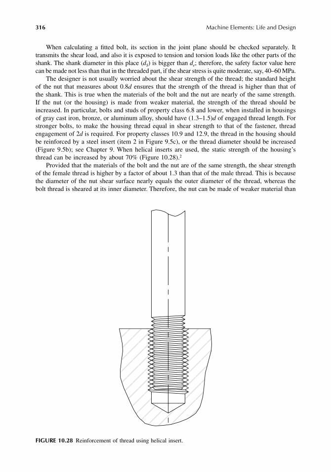
316 Machine Elements: Life and Design
When calculating a fitted bolt, its section in the joint plane should be checked separately. Ittransmits the shear load, and also it is exposed to tension and torsion loads like the other parts of theshank. The shank diameter in this place (dS) is bigger than de; therefore, the safety factor value herecan be made not less than that in the threaded part, if the shear stress is quite moderate, say, 40–60 MPa.
The designer is not usually worried about the shear strength of the thread; the standard heightof the nut that measures about 0.8d ensures that the strength of the thread is higher than that ofthe shank. This is true when the materials of the bolt and the nut are nearly of the same strength.If the nut (or the housing) is made from weaker material, the strength of the thread should beincreased. In particular, bolts and studs of property class 6.8 and lower, when installed in housingsof gray cast iron, bronze, or aluminum alloy, should have (1.3–1.5)d of engaged thread length. Forstronger bolts, to make the housing thread equal in shear strength to that of the fastener, threadengagement of 2d is required. For property classes 10.9 and 12.9, the thread in the housing shouldbe reinforced by a steel insert (item 2 in Figure 9.5c), or the thread diameter should be increased(Figure 9.5b); see Chapter 9. When helical inserts are used, the static strength of the housing’sthread can be increased by about 70% (Figure 10.28).2
Provided that the materials of the bolt and the nut are of the same strength, the shear strengthof the female thread is higher by a factor of about 1.3 than that of the male thread. This is becausethe diameter of the nut shear surface nearly equals the outer diameter of the thread, whereas thebolt thread is sheared at its inner diameter. Therefore, the nut can be made of weaker material than
FIGURE 10.28 Reinforcement of thread using helical insert.
9563_C010.fm Page 316 Monday, July 30, 2007 7:24 PM
Bolted Connections (BCs) 317
that of the bolt by the same factor 1.3. The weaker material of the nut enables better load distributionbetween the threads (because of plastic deformation of the nut material), and owing to this, itincreases the fatigue strength of the bolt. The useful height of the weaker nut can be increased to(1.4–1.6)d.
10.4.2 FATIGUE STRENGTH
Calculation of fasteners for fatigue strength is based on the mechanical properties of the materialand stress concentration factors, but the manufacturing technique also should be taken into con-sideration. For example, the bolt head formed by heading and the thread made by rolling arestronger than these elements formed by cutting.
The basics of calculations for fatigue strength are detailed in Chapter 12. As is shown there,the mean stress of the loading cycle affects the fatigue strength very little. As applied to fasteners,the influence of the mean stress can be neglected completely unless the maximal stress is lowerthan 0.9Sy. So the only force to be taken into consideration in the calculation for endurance is theamplitude of the working (alternating or variable) load Faw. Because the bolt “feels” only a portionof the working load, the amplitude of the bolt force Fab can be obtained as follows:
(about coefficient χ see Subsection 10.3.1).The nominal stress amplitude σa equals
(10.15)
where A = area of the section under consideration (mm2).Comparing Equation 10.15 with Equation 10.14, we notice that coefficient 1.3 has disappeared.
This is not a mistake. In the endurance calculation, we consider only the variable load. But thetorque induced in the bolt shank while tightening doesn’t change, and it can’t influence the fatiguestrength of the shank. But it does influence the maximal stress, which should not exceed the limitmentioned earlier.
There are two areas in the bolt that should be checked for fatigue strength: transition from theshank to the bolt head, and also the threaded part. Usually a fatigue crack originates in the area ofthe most heavily loaded thread. In this place, the stress caused by tension of the shank is supple-mented with stress induced by bending of the thread profiles (Figure 10.29). The latter is responsiblefor the low fatigue strength of the threaded shank: experiments show2 that without bending, thefatigue limit of a tensioned threaded rod increases threefold. This factor can hardly be calculated;therefore, the admissible amplitude of the variable tensile stress is usually recommended on thebasis of experiments. As a guide, for rolled threads, the admissible value of σa can be estimatedfrom the following equation:8
whereSu = tensile strength of the material (MPa)d = thread diameter (mm)ξ = 0.15 for steels with Su ≤ 1100 MPa
F F Nab aw= ⋅ χ
σaabF
AMPa=
σ ξa uSdd
= ++
2525 3
9563_C010.fm Page 317 Monday, July 30, 2007 7:24 PM

318 Machine Elements: Life and Design
Example: for bolt M16–10.9 (Su = 1040 MPa)
Another manual9 recommends σa = 65–85 MPa at Su = 600–1200 MPa, if the bolt is heat-treated before rolling the thread. With the same conditions for a cut thread, σa = 55–70 MPa isrecommended. Because the fatigue strength of the thread displays significant dependence onmanufacturing processes, in important cases, the admissible amplitude of the tensile stress shouldbe determined experimentally. To obtain true results in the experiments, not only the bolt (or stud)but also the adjoined parts should be similar to the real ones, because they also influence the loadcapacity of the bolt. For instance, weaker nut materials, as well as materials with smaller modulusof elasticity, contribute to better load distribution in the thread, decrease the bending load on themost loaded threads, and increase the fatigue strength of the bolt.
A very effective idea may be to increase the radius in the root of the thread (say, to r = 0.2p,where p is the pitch of thread). The endurance of the threaded parts can also be improved byincreasing manufacturing and assembly accuracy and decreasing clearances. Small clearancesrestrict the bending deformation of the threads.
Another area to be assessed for strength is the fillet that makes the transition from theshank to the head of the bolt. Increase in the fillet radius is limited by the loss in the bearingsurface of the head; therefore, elliptic fillets are often used for heavily loaded bolts, as shownin Figure 10.30. Because there is only one stress raiser (fillet) with a well-known influence
FIGURE 10.29 Bending of threads.
FIGURE 10.30 Bolt designed for high fatigue strength.
BoltHousing (nut)
σa MPa= ⋅ ++ ⋅
=0 15 104025 16
25 3 1687 6. .
9563_C010.fm Page 318 Monday, July 30, 2007 7:24 PM

Bolted Connections (BCs) 319
on the maximal stress, calculations in relation to this area are performed by conventionalmeans (see Chapter 12).
REFERENCES
1. Seidel, M. and Schaumann, P., Measuring of Fatigue Loads of Bolts in Ring Flange Connections,EWEC 2001 Conference, Copenhagen, 2001.
2. Birger, I.A. and Iosilevich, G.B., Threaded Joints, Mashinostroenie, Moscow, 1973 (in Russian).3. Gati, T., Evaluation of Stresses, Strain and Displacements in Bolted Joints, Master’s thesis, Ben-
Gurion University of the Negev, Beer-Sheva, 2003 (in Hebrew).4. Gorbunov, M.N. and Saltikov, M.A., Calculation of Flange Connections of Shafts with Fitted Bolts
under Varying Torsion, Energomashinostroenie, 1973/12 (in Russian).5. Saltikov, M.A. and Gorbunov, M.N., Method of Strength Evaluation of Detachable Connections,
Mashinostroenie, Moscow, 1983 (in Russian).6. Bossard Ltd. Fasteners, Metric Fasteners for Advanced Assembly Engineering, Catalogue and
technical information YB.7. Timoshenko, S., Vibration Problems in Engineering, D. Van Nostrand Company, Toronto, New York,
London, 1955.8. Heywood, R.B., Designing Against Fatigue of Metal, Reinhold, New York, 1962.9. Birger, I.A., Shorr, B.F., and Iosilevich, G.B., Calculation of Machine Elements for Strength. Manual,
Mashinostroenie, Moscow, 1979 (in Russian).
9563_C010.fm Page 319 Monday, July 30, 2007 7:24 PM

9563_C010.fm Page 320 Monday, July 30, 2007 7:24 PM

321
11
Connection of Units
Machines are usually divided into units (subassemblies) that are manufactured separately and thenlinked together. This method of forming machines has many points in its favor, and some of themdeserve to be mentioned.
1. Manufacturing and quality inspection of each unit can be performed separately andsimultaneously, reducing the time taken to make the machine.
2. Partitioning of machines into units enables standardization and use of the standard unitsin different machines. As an illustration, we can refer to electric motors, gearboxes,couplings, high-pressure fuel pumps and injectors for diesel engines, and infinitely manyother units. It is impossible to imagine modern technical civilization without thiscomprehensive unification and standardization.
3. When a machine fails, it is the work stoppage, not the repair, that usually is mostexpensive. The failed machine can disable a production conveyer or the entire plant.Replacing a failed unit by a new one warehoused as a spare can reduce the repair timeto a minimum.
4. Use of units facilitates the task of machine designers who can compound their machinesfrom stock-produced “cubes,” linking them in the needed way.
If a machine has a part that, because of shorter service life or for some other reasons, will needto be periodically replaced, it should be segregated into an easily detachable unit to shorten theservice interruption.
Sometimes the interruption time can be critical when trying to avoid very serious and evencatastrophic consequences. In such cases, the equipment should be built so that when the primarymachine fails, the reserve machine, which is permanently connected and kept in operating condition,starts automatically and immediately.
The stock-produced units have elements for connection to other units, like flanges, spigots,mounting feet, threads, and others. Their dimensions are given in the manufacturer’s catalogs alongwith other technical data. In many cases, there are given several options of attachment, andsometimes a special design of the attachment elements is available, when it is economically feasible.
Connection of two units consists of housing connections and, separately, connection of partstransmitting motion, which are mostly rotating shafts.
11.1 HOUSING CONNECTIONS
Housings can be connected directly or through an intermediate part, like a frame or foundation.The direct connection is cheaper. Figure 7.30 shows a direct connection of electric motor 7 throughadapter 8 to the housing of the gear. Another example of direct connection is shown in Figure 7.31.Oil pump 1 is connected to the upper bearing cup, and electric motor 8 is attached to extension 9of the upper part of the gear housing. (Openings 10 are made to ventilate the coupling chamberand to inspect the condition of the rubber elements of the coupling.)
If the attached unit is relatively large and weighty, it can induce remarkable deformations inthe housing and bring about misalignment of the teeth and bearings of the gear. The possibledeformations can be calculated using FEM. The stock-produced units don’t always have attachment
9563_C011.fm Page 321 Wednesday, July 25, 2007 4:37 PM
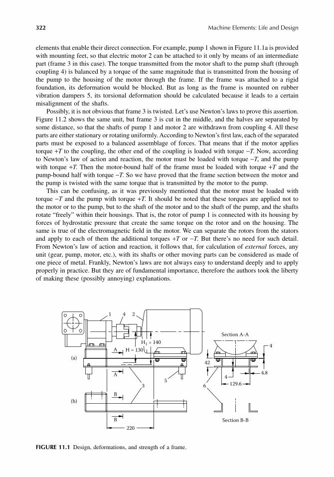
322
Machine Elements: Life and Design
elements that enable their direct connection. For example, pump 1 shown in Figure 11.1a is providedwith mounting feet, so that electric motor 2 can be attached to it only by means of an intermediatepart (frame 3 in this case). The torque transmitted from the motor shaft to the pump shaft (throughcoupling 4) is balanced by a torque of the same magnitude that is transmitted from the housing ofthe pump to the housing of the motor through the frame. If the frame was attached to a rigidfoundation, its deformation would be blocked. But as long as the frame is mounted on rubbervibration dampers 5, its torsional deformation should be calculated because it leads to a certainmisalignment of the shafts.
Possibly, it is not obvious that frame 3 is twisted. Let’s use Newton’s laws to prove this assertion.Figure 11.2 shows the same unit, but frame 3 is cut in the middle, and the halves are separated bysome distance, so that the shafts of pump 1 and motor 2 are withdrawn from coupling 4. All theseparts are either stationary or rotating uniformly. According to Newton’s first law, each of the separatedparts must be exposed to a balanced assemblage of forces. That means that if the motor appliestorque
+
T
to the coupling, the other end of the coupling is loaded with torque
−
T
. Now, accordingto Newton’s law of action and reaction, the motor must be loaded with torque
−
T
, and the pumpwith torque
+
T
. Then the motor-bound half of the frame must be loaded with torque
+
T
and thepump-bound half with torque
−
T
. So we have proved that the frame section between the motor andthe pump is twisted with the same torque that is transmitted by the motor to the pump.
This can be confusing, as it was previously mentioned that the motor must be loaded withtorque
−
T
and the pump with torque
+
T
. It should be noted that these torques are applied not tothe motor or to the pump, but to the shaft of the motor and to the shaft of the pump, and the shaftsrotate “freely” within their housings. That is, the rotor of pump 1 is connected with its housing byforces of hydrostatic pressure that create the same torque on the rotor and on the housing. Thesame is true of the electromagnetic field in the motor. We can separate the rotors from the statorsand apply to each of them the additional torques
+
T
or
−
T
. But there’s no need for such detail.From Newton’s law of action and reaction, it follows that, for calculation of
external
forces, anyunit (gear, pump, motor, etc.), with its shafts or other moving parts can be considered as made ofone piece of metal. Frankly, Newton’s laws are not always easy to understand deeply and to applyproperly in practice. But they are of fundamental importance, therefore the authors took the libertyof making these (possibly annoying) explanations.
FIGURE 11.1
Design, deformations, and strength of a frame.
(a)
Section A-A
A
A
B
B
(b)
Section B-B
1 4 2
35
6
H1 = 140
H = 130
129.6
4
4
4.8
42
220
9563_C011.fm Page 322 Wednesday, July 25, 2007 4:37 PM

Connection of Units
323
E
XAMPLE
11.1
Let’s calculate the deformations of the frame shown in Figure 11.1. Pump 1 is driven by electricmotor 2. Their housings are connected through frame 3 and the shafts through coupling 4. Theframe is installed on four dampers 5. The motor power
P
=
3 kW at
n
=
1425 r/min, so the torque
T
is given by:
The frame is mainly made of two aluminum equilateral angle bars 6 (38
×
38
×
4.8 mm). Twoversions of the frame are represented in Figure 11.1:
1. The angle bars are covered with plates of 4 mm thickness from above and below, alongtheir whole length (section A-A).
2. The middle part of the frame is left without covering, and only the angles transmit thetorque between the housings of the motor and the pump (section B-B).
To calculate approximately the frame deformation, we can consider the plated ends (under themotor and the pump) as completely rigid, and take into account only the middle part of the framethat is 220 mm long. The dimensions of the frame are given in Figure 11.1.
Figure 11.3a shows the simplified cross section of version a. For our calculations, we take it asa hollow rectangle, because we have formulas for this shape. The angle of torsion
ϕ
of this section is:
where
T
=
torque (N·mm)
L
=
length of the twisted part (L
=
220 mm)
G
=
shear modulus (G
=
0.28·10
5
MPa for aluminum alloy)
J
=
polar moment of inertia (mm
4
) that equals for this section
1
FIGURE 11.2
Twisting of the frame.
+T
−T −T
−T
+T
1 4 2
3
+T
TPn
N m= = = ⋅9555 95553
142520 1.
ϕ = ⋅⋅
T LJ G
Jt t a b
at b t=
+= ⋅ ⋅ ⋅ ⋅
⋅2 2 4 8 4 124 8 38
124 81 2
2 2
1 2
2 2. .. 44 8 38 4
1 15 106 4
..
+ ⋅= ⋅ mm
9563_C011.fm Page 323 Wednesday, July 25, 2007 4:37 PM
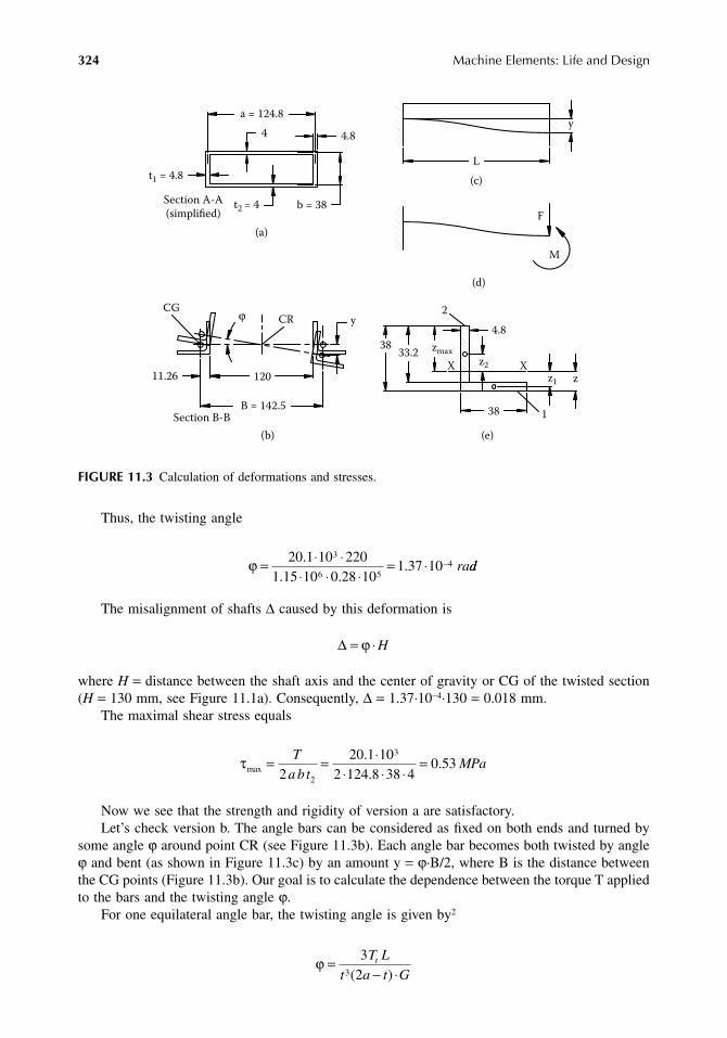
324
Machine Elements: Life and Design
Thus, the twisting angle
The misalignment of shafts
∆
caused by this deformation is
where
H
=
distance between the shaft axis and the center of gravity or CG of the twisted section(
H
=
130 mm, see Figure 11.1a). Consequently,
∆
=
1.37·10
−
4
·130
=
0.018 mm.The maximal shear stress equals
Now we see that the strength and rigidity of version a are satisfactory.Let’s check version b. The angle bars can be considered as fixed on both ends and turned by
some angle
ϕ
around point CR (see Figure 11.3b). Each angle bar becomes both twisted by angle
ϕ
and bent (as shown in Figure 11.3c) by an amount y
=
ϕ
·B/2, where B is the distance betweenthe CG points (Figure 11.3b). Our goal is to calculate the dependence between the torque T appliedto the bars and the twisting angle
ϕ
.For one equilateral angle bar, the twisting angle is given by
2
FIGURE 11.3
Calculation of deformations and stresses.
CG
Section B-B
(b)
CRϕ
(c)
L
(d)
(a)
F
M
(e)
X z2
z1 zX
138
2
zmax
Section A-A
(simplified)
t1 = 4.8
a = 124.8
4 4.8
b = 38t2 = 4
11.26
y
3833.2
B = 142.5
120
4.8
y
ϕ = ⋅ ⋅⋅ ⋅ ⋅
= ⋅ −20 1 10 2201 15 10 0 28 10
1 37 103
6 54
.. .
. radd
∆ = ⋅ϕ H
τmax
..
.= = ⋅⋅ ⋅ ⋅
=Ta bt
MPa2
20 1 102 124 8 38 4
0 532
3
ϕ =− ⋅
323
T L
t a t Gt
( )
9563_C011.fm Page 324 Wednesday, July 25, 2007 4:37 PM

Connection of Units
325
where
T
t
=
twisting torque of one bar (N·mm)
L
=
length of the bar (
L
=
220 mm)
t
=
thickness of the angle’s webs (i.e., its legs) (
t
=
4.8 mm)
a
=
lateral length (
a
=
38 mm)
G
=
shear modulus (
G
=
0.28·10
5
MPa for aluminum alloy).
From here,
(11.1)
The resistance forces created by bending can be calculated using a scheme shown in Figure 11.3d,where, on one side, the fixing is substituted by overhang force
F
and bending moment
M
. Theseforces can be defined as follows (assuming that the deflection y is known):
The bending angles on the end of a beam caused by force
F
(
θ
F
) and by moment
M
(
θ
M
) areas follows:
where
E
=
modulus of elasticity (E
=
0.72·10
5
MPa for aluminum alloy)
I
=
moment of inertia of the cross section (mm
4
)
As the resultant angle at this point is zero,
(11.2)
The deflections of the beam end caused by force
F
(
y
F
) and by moment
M
(
y
M
) are
As the resultant deflection at this point equals
y
,
(11.3)
After insertion of Equation 11.2 into Equation 11.3, we obtain the following:
(11.4)
Tt a t G
Lt = − ⋅ϕ3 2
3( )
Θ ΘF M
F LE I
M LE I
= − =2
2;
Θ ΘF M
F LE I
M LE I
MF L
+ = − + =
=
2
20
2
;
yF LE I
yM l
E IF M= = −3 2
3 2;
y yF LE I
M LE I
yB
F M+ = − = =3 2
3 2 2ϕ
ϕ = F LE I B
3
6
9563_C011.fm Page 325 Wednesday, July 25, 2007 4:37 PM

326
Machine Elements: Life and Design
The resistance torque (
T
b
) caused by the bending deformation of the angle bars equals
Inserting
F
=
T
b
/B into Equation 1.4, we obtain the following:
(11.5)
The summary resistance torque, which equals the applied torque of the motor T, is obtainedfrom Equation 11.1 and Equation 11.5:
(11.6)
Here, λ is equal to the expression in parentheses.All the terms of Equation 11.6 are already known from the preceding text except the moment
of inertia I. It is well known how to determine the I value; it is given in the catalog. But the authorsare glad to demonstrate this process for the case of nonstandard profile. The steps are as follows:
1. Inasmuch as the beam is bent in the vertical plane, we are to define the value of I abouta horizontal axis x–x passing through the CG of the cross section (to obtain the minimalvalue of I).
2. The cross section of the bar is shown in Figure 11.3e. To ease our work, we divide thecross section into two rectangles 1 and 2. Each of them has its own CG obviously placedin its geometric center (marked by a small circle). The area of rectangle 1, A1 = 38·4.8 =182.4 mm2 and that of rectangle 2, A2 = (38 − 4.8)4.8 = 159.36 mm2.
3. To determine the position of the x–x line, let’s put it at a coordinate z. Then the distancesof the CGs of rectangles 1 and 2 from the x–x line are equal respectively to z1 = (z − 2.4)mm and z2 = 38 − z − 16.6 = (21.4 − z) mm.
4. The equilibrium equation is
5. Now we can calculate the I value from the following formula:
T F Bb = ⋅
TB E ILb = ϕ 6 2
3
T T Tt a t G
LB E ILt b= + = − +
= ⋅22 2
363 2
3ϕ ϕ λ( )
A z A z
z z
z
1 1 2 2
182 4 2 4 159 36 21 4
=
− = −
;
. ( . ) . ( . )
where == = =11 26 8 86 10 141 2. . .mm z mm z mm
I I A z
I mm I
i i i= +( )
= ⋅ = = ⋅
Σ 2
1
34
2
38 4 812
350 24 8 3.
. ;. 33 2
1214638
350 2 14638 182 4 8 86 1
34
2
.
. . .
=
= + + ⋅ +
mm
I 559 36 10 14 456922 4. .⋅ = mm
9563_C011.fm Page 326 Wednesday, July 25, 2007 4:37 PM

Connection of Units 327
Coming back to Equation 11.6, we obtain the λ value:
(Note that in the equation for λ, the first term is negligible as compared with the second one, whichmeans that in this case, when the angle bars are distanced from each other, their twisting deformationis relatively small and can be neglected.)
The distance between the motor axis and the CR of the angle bars H1 = 140 mm (see Figure11.1a). Consequently, the shaft misalignments caused by the frame deformation is
The stresses in the angle bars can be calculated separately from torsion and from bending andthen combined. The torque can be calculated using Equation 11.1:
The maximal shear stress
The maximal bending moment can be obtained from Equation 11.2 and Equation 11.4:
The maximal bending stress
(Regarding zmax, see Figure 11.2e.)The maximal equivalent stress
It is a very small stress (see, for instance, the data in Table 9.1). But the misalignment of 0.074 mmis noticeable.
λ = − + = ⋅ ⋅ − ⋅2 23
6 2 4 8 2 38 4 8 0 23 2
3
3t a t G
L
B E I
L
( ) . ( . ) . 88 103 220
6 142 5 0 72 10 4220
6 6
5 2 5
3
⋅⋅
+ ⋅ ⋅ ⋅ ⋅
=
. .
. 88 10 376 4 10 3 83 10
201003 8
5 5 7⋅ + ⋅ = ⋅ ⋅
= =
. . ;
.
N mm
Tϕλ 33 10
5 25 107
4
⋅= ⋅ −. rad
∆ = ⋅ = ⋅ ⋅ =−ϕ H mm145 25 10 140 0 074. .
Tt a t G
Lt = − ⋅ = ⋅ ⋅ − ⋅−ϕ3
432
35 25 10
4 8 2 38 4 8 0( ).
. ( . ) .228 103 220
1755⋅
⋅= ⋅N mm
τmax ( ) . ( . ).=
−= ⋅
⋅ −=3
23 175
4 8 2 38 4 80 32
2 2
T
t a tMPt aa
ME I BL
= = ⋅ ⋅ ⋅ ⋅ ⋅−ϕ 35 25 10
3 0 72 10 45692 142 5222
45
.. .
0015255
2= ⋅N mm
σmax max . .= = =MI
z MPa1525545692
26 74 8 93
σ σ τe MPa= + = + ⋅ =max max . . .2 2 2 24 8 93 4 0 32 8 95
9563_C011.fm Page 327 Wednesday, July 25, 2007 4:37 PM

328 Machine Elements: Life and Design
Connection of units through an intermediate frame or foundation can also be forced by a heavyweight of the equipment that must be installed on a rigid horizontal foundation, as well as bygreater distance between the units that makes impracticable the direct connection of the housings.But, anyway, we have to remember that the frames and foundations are not just supports. They areparts of a mechanism that participate in load transmission, and they must be checked for strengthand deformations like other parts. The only difference is that these parts are stationary and madeof cheaper materials, so their safety factors can be much greater and the calculations respectivelymore approximate.
EXAMPLE 11.2
Figure 11.4 shows a foundation made for a proving stand for escalator drive units. Drive unit1 is linked to block brake 2 by chain 3. The forces given in Example 4.5 and Figure 4.20 arevalid for an escalator in service. When testing, the weight of the hauling chains is negligible,and only the difference between forces Fcu and Fcl, which creates the torque on the main shaft,is realized:
Force F is applied to both the drive unit 1 and the brake 2 at a height of 2.5 m from thefoundation surface. As the foundation height measures 2 m, the arm of force F (its distance to theneutral line (0-0) equals 3.5 m, and the bending moment M applied to the foundation is as large as
FIGURE 11.4 Foundation for proof test of escalator drive unit.
F F F Ncu cl= − = − = ⋅300 000 100 000 2 105, ,
M N mm= ⋅ ⋅ = ⋅ ⋅2 10 3500 7 105 8
20000
2500
132
5
4
F F
9563_C011.fm Page 328 Wednesday, July 25, 2007 4:37 PM
Connection of Units 329
The main shaft of the escalator is provided with two sprockets (see Figure 4.20), but for thetrials, only one of them (near the gear) is linked to the brake. This leads to uneven distribution ofthe bending moment across the width of the foundation. The factor of this unevenness can begenerously taken as k = 2 (as only one of the two sprockets transmits the load).
Now we can calculate the stress in the foundation. Its cross section is 2 m high and 3 m wide.The bending stress
The ultimate bending stress of concrete (of medium quality) is about 3 MPa (on the tensionside), so the safety factor SF is given by
As shown in Figure 11.4, the concrete foundation is reinforced by a welded structure 4 madeof rectangular tubes. The vertical members of the structure are provided with thick plates 5 withthreaded holes for attachment of equipment. The structure has been aligned, welded, and theninstalled in a pit with a form and filled with concrete.
The bending deformations of the concrete foundation, in this case, are relatively small, andthey don’t influence anything.
These two examples demonstrate the idea that whatever the design and the materials of theframe or the foundation, they can’t be considered as completely rigid and infinitely strong. Theirstrength and deformations are worth checking, even if they look massive and reliable.
It is undesirable to install two connected machines on separate foundations, as in this case, theearth between the foundations is included in the chain of parts transmitting the load. The possiblealteration in the relative placement of the connected units must be taken into consideration whenchoosing the kind of connecting couplings.
11.2 SHAFT CONNECTIONS
11.2.1 ALIGNMENT OF SHAFTS
A student of history once asked his professor: “Sir, you told us about World War II. Does it meanthat there was also a World War I?” So, before discussing the alignment of shafts, we will studywhat misalignment is and why it may cause problems.
Misalignment of shafts is an offsetting of their axes. Figure 11.5a shows the condition calledradial misalignment; the axes of the shafts remain parallel, but they are displaced relative to eachother by an amount e in the radial direction. Shafts 1 and 2 are joined together by bolts. If theshafts and their supports were absolutely rigid, the fixed joint would not allow the shafts to rotate.But the parts are resilient, and the bearings have clearances, so the shafts can rotate by applicationof a certain torque. These shafts, turned by 180°, are shown in Figure 11.5b. The shafts are quitebent, and the bearings are loaded in proportion to the bending forces.
EXAMPLE 11.3
Let’s calculate these forces, assuming that the shafts are identical and their dimensions are d =80 mm, C = 160 mm, L = 400 mm, and e = 0.3 mm. To be turned by 180°, the shafts must bedeformed in total by 2e = 0.6 mm, that is, each shaft by 0.3 mm (because the shafts are identical;
σ =⋅
= ⋅⋅
=Mb h
k N mm6
7 106
3000 20002 0 7
28
22. /
SF = =30 7
4 3.
.
9563_C011.fm Page 329 Wednesday, July 25, 2007 4:37 PM

330 Machine Elements: Life and Design
if not, the total deformation of 0.6 mm would be distributed between the shafts in proportion totheir compliance). The shaft end deflection y under an overhang force F equals
whereE = 2.06·105 MPa (modulus of elasticity)I = moment of inertia of the shaft cross section
From here,
The additional load Fadd applied to the nearest bearing
The additional bending moment Madd to which the shaft is exposed due to force F is given by
FIGURE 11.5 Effect of radial misalignment on shaft and bearing loads.
(a)
(b)
1 2L C
d
e
yF C
E IL C mm= ⋅ +
2
3( )
Id
mm= = ⋅ = ⋅π π4 46 4
6480
642 01 10.
y F=⋅ ⋅ ⋅ ⋅
+ = ⋅1603 2 06 10 2 01 10
400 160 1 15 102
5 6. .( ) . −− =
= ⋅
5
4
0 3
2 6 10
F mm
F N
.
.
F FL C
LNadd = + = ⋅ + = ⋅2 6 10
400 160400
3 64 104 4. .
M F C N mmadd = ⋅ = ⋅ ⋅ = ⋅ ⋅3 64 10 160 5 82 104 6. .
9563_C011.fm Page 330 Wednesday, July 25, 2007 4:37 PM

Connection of Units 331
Consequently, the additional cyclic bending stress σadd is as follows:
This calculation is made on the assumption that the shaft supports are gapless and absolutelyrigid. If these factors were taken into account, force F would be somewhat less, but the consequencesof the misalignment remain harmful. In addition to the increased bending stresses in the shaft, itselastic deformation and dislocation with respect to the housing may lead to the misalignment ofthe parts of the mechanism and to its premature failure.
Figure 11.6 shows angular misalignment characterized by angle γ. The shafts, each with twosupports, are bolted together at the flange connection. As a result of these constraints, both shaftshave become bent. If the two outer supports were removed and the shafts rotated by 180°, theywould take up the position shown with dashed lines in Figure 11.6b.
There can also be combined misalignment, both radial and angular. The effect of this misalign-ment is similar to that described previously. These deformations and loads change cyclically, andthey must be held relatively small to prevent increased noise, vibrations, and overload of the machineelements. Imparting the optimum alignment has the objective of making the shafts coaxial, therebydiminishing the additional forces and deformations that can be avoided just by fair adjustment.
In the technical literature, axial misalignment is also mentioned. Here it is not consideredbecause the so-called axial misalignment is just the variation of axial distance between the connectedshafts. If this distance changes within limits, admissible by the design of bearings and couplings,this has no influence on the working conditions of the mechanism, independent of the kind ofcoupling, whether it is rigid or resilient. The designer can increase the admissible limits of axialdisplacement of the shafts relative to each other, so that the procedure of installation in the axialdirection doesn’t cause any trouble. In some cases, the temperature expansion of the shafts shouldbe kept in mind.
The achievable accuracy of adjustment depends not only on the instruments used, but also onthe design of the shafts to be aligned and their supports. Let’s consider coaxiality of two gears
FIGURE 11.6 Effect of angular misalignment on shaft and bearing loads.
σadd
M dI
MPa= = ⋅ ⋅⋅ ⋅
=2
5 82 10 802 2 01 10
1166
6
..
(a)
(b)
1 2γ
9563_C011.fm Page 331 Wednesday, July 25, 2007 4:37 PM

332 Machine Elements: Life and Design
shown in Figure 5.23 or, the same, in Figure 6.43. The bearings of these gears are coaxial and thegears, when unloaded, are coaxial as well (within close manufacturing tolerances). But under aload, the gears move in the bearings within the clearances in different (possibly, in opposite)directions. If we knew exactly the position of the gears while the machine is operating, we wouldjust displace the bearings by a calculated amount and have achieved the exact alignment. As theoperating regime is varying, the position of the shafts, as well as their alignment changes in responseto the variable conditions.
Another problem of alignment is the possible instability of the connection between the hous-ings. For example, if the engine is installed on dampers (this is usual in seaborne machinery), itcan move by millimeters from its nominal position depending on the torque transmitted and onthe inertia forces caused by the motion of the ship in the sea. The ship’s hull may also haveconsiderable deformations, both momentary (caused by heavy seas, cargo placement, etc.) andpermanent (resulting from release of the internal stresses in the welded hull). (Submarines haveespecially challenging alignment requirements due to hull deflections that occur due to diving andsurfacing and from the effects of high-speed maneuvering.) This is the problem; alignment canonly be directly performed and checked during assembly, while the shafts are coaxial under idealrunning conditions. The quality of the alignment can be checked only indirectly by measuringnoise and vibrations. To properly predict alignment in operation, the weight of parts, workingforces, as well as the temperature and other kinds of influence on deformations must be consideredwhen planning the alignment procedure. For example, Figure 11.7a shows a shaft of a large electricgenerator bent by the weight W of the rotor. In operation, this force remains and no other forceis added, so the alignment of this shaft can be made just as is, i.e., the housing should be tiltedas shown in Figure 11.7b.
A pinion-shaft with an overhanging flywheel is shown in Figure 11.7c unloaded (W is theweight of the flywheel and the pinion shaft together) and in Figure 11.7d under load (FW is theworking force). In this case, the angles α and β and the radial displacements in two perpendicularplanes (e.g., horizontal and vertical) should be calculated. Then the alignment at rest can beoptimized, taking into account the gravity load and the operating loads.
Figure 11.7e and Figure 11.7f show a less complicated case. Here, the shaft is rigid enough,but the working force FW is directed nearly opposite to the weight. In that case, a certain calculatedmisalignment of the shafts must be set during the alignment procedure to take into account thevertical and lateral displacements of the shaft in the bearings during operation.
FIGURE 11.7 The influence of weight and working forces on shaft alignment.
W
W
Wα
W
β
FW
(a)
(b) (d)
(c)
(f )
FW
W
(e)
W
9563_C011.fm Page 332 Wednesday, July 25, 2007 4:37 PM

Connection of Units 333
In smaller machines, these difficulties don’t exist as a rule, because the clearances in the rollingbearings and the elastic deformations of the parts are relatively small, and the widely used couplingshave the ability to compensate for some moderate misalignment.
Figure 11.8 shows how the misalignment is usually measured. If the neighboring parts of theshafts (flanges or half-couplings) are precisely machined, the misalignment can be measured asshown in Figure 11.8a and Figure 11.8b. The radial misalignment e is given by
e = A = B mm
The angular misalignment γ is given by
Dimensions A, B, C, and D can be measured by a feeler gauge or caliper (depending on theneeded accuracy). Figure 11.8c and Figure 11.8d show the application of a pointer-type indicatorto the alignment measurements. If the surfaces used for alignment are exact, relative to the related
FIGURE 11.8 Alignment techniques.
(b)
(a)
(e)
1 2
ee e
3
(d)
(c)
Bench rule
A
e
B
C
Dd
d
γ = −C Dd
rad
9563_C011.fm Page 333 Wednesday, July 25, 2007 4:37 PM

334 Machine Elements: Life and Design
shafts (that means, their radial and lateral runouts are negligible as compared to the admissiblemisalignment), the alignment operation can be performed by the rotation of one shaft only. But ifthese surfaces are not exact, both shafts should be rotated together, so that the test point of theindicator touches the mating shaft nearly at the same point throughout the alignment operation.
As shown in Figure 11.8e, the angular misalignment is accompanied by radial misalignment,changing along the axis. It is often important to measure the radial misalignment in a certain placedepending on the kind of coupling. For example, in the coupling shown in Figure 11.11, it isimportant to maintain concentricity between rubber sleeves 4 and pockets in half-coupling 2.Therefore, in this case, the radial displacement should be measured in the middle plane of therubber sleeves. As the radial alignment changes with the angular alignment, the latter alignmentshould be adjusted first.
While measuring the angular misalignment, the shafts must not have any axial motion relativeto each other. That should be ensured and checked.
11.2.2 RIGID COUPLINGS
The most widespread rigid coupling is just a plain flange connection. The flange can be made asan integral part of the shaft or manufactured separately and connected to the shaft by one of thenumerous methods that have been partly described in Chapter 5.
Another kind of rigid coupling is a sleeve connected to both shafts by hydraulically assembledpress fit (Figure 5.2a) or by key (Figure 11.9). In the last case, the sleeve should be slide fitted tothe shafts (otherwise it can hardly be assembled or dismantled). Therefore, it can be applied tolight-duty loads only (see Subsection 5.1.2).
The rigid couplings, in effect, convert the pair of shafts into a single four-bearing shaft, andthis demands proper placement of all four bearings. In many cases, “proper placement” means thatthe bearings should be coaxial. But it is not always so.
One popular type of rigid connection is the male/female attachment, where one unit with ahollow shaft is mounted on the solid shaft of another unit. Figure 11.10 shows the connection ofa gear motor 1 to a driven machine 2. The hollow output shaft of the gear motor is assembled with
FIGURE 11.9 Sleeve coupling.
Wrong option
Better
9563_C011.fm Page 334 Wednesday, July 25, 2007 4:37 PM

Connection of Units 335
the shaft of the driven machine with a key and transition fit. The housing of the gear motor is fixedagainst rotation by the bolt connection of lug 3 to bracket 4. Force F applied to the lug of the gearhousing equals
where T = torque on the output shaft of the gear.Let’s use our right to transfer force F from lug 3 to the point over the shaft (to position F*)
with the addition of torque T. Force F is applied to the lug that is a part of the housing. Hence,force F* must be applied to the housing as well. The reaction of the driven machine shaft (−F*)is applied to the hollow shaft and directed upwards, whereas the tooth force Ft applied to the outputgear and shaft is directed nearly downwards. Thus, when determining the load on the output shaftbearings, force F* must be subtracted from force Ft. Direction and magnitude of force F* dependson the placement and inclination angle of lug 3, and the designer can try some options.
The bending moment M applied to the driven shaft in its most stressed section is given by
FIGURE 11.10 Shaft-mounted gear motor.
4
K
2
1
3
L
F
−F∗
Ft
3
F∗
T
FTL
=
M F KT K
L= ⋅ = ⋅
9563_C011.fm Page 335 Wednesday, July 25, 2007 4:37 PM

336 Machine Elements: Life and Design
Dimension K is shown in Figure 11.10. The lesser this dimension, the smaller the bendingmoment.
11.2.3 RESILIENT COUPLINGS
In many cases, it is impracticable to achieve ideal alignment of the shafts because of many influencesthat are not exactly known, for the most part, and changing with time, like loads, temperaturedeformations, wear of the bearings, and others. But as is evident from the foregoing, any kind ofmisalignment of rigidly connected shafts leads to their cyclic deformation and possible overstress.The purpose of resilient couplings is to shift the deformation from the shafts, which are made ofsteel and therefore very rigid, to some intermediate resilient element that can be deformed byrelatively small forces and decreases the additional load of the shafts. But this element, usuallymade of elastomers (rarely of steel springs), has to transmit torque from one shaft to another.Because of this, the resilient element is placed between (or attached to) two metal parts, that arein turn connected to the shafts. The unit formed by two metal parts and elastomeric intermediateparts is called a resilient coupling.
In addition to compensation of shaft misalignment, couplings of this kind are able to dampimpact loads, vibrations, and oscillations. Change of the material and configuration of the elasto-meric elements enables wide variation of the coupling stiffness; this can be useful to change thenatural frequency of the entire shafting system. Due to the nonlinearity of their stiffness, resilientcouplings can prevent the development of resonance.
These couplings are relatively cheap and don’t need any maintenance. In some cases, theirelectrical insulating properties and structural noise damping are of value.
There are many resilient couplings, different in design. Figure 11.11 shows a coupling withpins and compressed rubber sleeves. Half-couplings 1 and 2 are connected to the shafts by tightfits and keys. Pins 3 with rubber sleeves 4 are attached to half-coupling 1 by their tapered endsand tightened with a nut. The rubber sleeves enter pockets in half-coupling 2, and in this way, thetorque is transmitted from one shaft to another. It is clear that if the load is evenly distributedbetween the pins, the vector sum of the pin forces equals zero, and no shaft bending is caused bythe coupling. The compliance of the pins and, mainly, of the rubber sleeves makes it possible tokeep a more or less even load distribution between the pins at a moderate misalignment, and theradial forces, which bend the shaft, can be kept relatively small.
Figure 11.12 shows another design of flexible coupling. Half-couplings 1 and 2 are identical(section A-A shows them separated). The protrusions of one of them enter the recesses of the other,and rubber spider 3 is installed between them, so that the torque can be transmitted from onehalf-coupling to another through the spider only. Depending on the direction of torque, half of thespider’s blades are loaded in compression, and the other half are idling.
FIGURE 11.11 Flexible coupling with pins and rubber sleeves.
A
Section A-A
2 1
34A
9563_C011.fm Page 336 Wednesday, July 25, 2007 4:37 PM

Connection of Units 337
A resilient coupling with rubber pads is presented in Figure 11.13. This design is usually usedfor large torques, because half-couplings 1 and 2 can be made very strong and large enough indiameter, so that the number of the pads can be increased as needed. The same rubber pads canbe used for different diameters due to conformable shaping of the blades. As in the previous case,only half of the pads transmit the load, whereas the other half are idling. If the torque is nonreversing,the idling pads can be made thinner, and therefore more pads can be used.
The load capacity of the couplings shown in Figure 11.11 through Figure 11.13 is limited bythe permissible pressure on the elastomeric elements. Depending on the hardness of the polymer,it varies from 2–3 MPa. So the increase in quantity of the elements enables a decrease in theirdimensions or a decrease in the diameter of the coupling.
The considered couplings can compensate for radial misalignment of about 0.1 mm/100 mmof their outer diameter and an angular misalignment of approximately 1°. It doesn’t mean that thesevalues of misalignment are permissible for the alignment operations. Figure 11.14 demonstrates the
FIGURE 11.12 Flexible coupling with an elastomeric spider.
FIGURE 11.13 Flexible coupling with rubber pads.
Section A-A1
2
1 2
3A
A
Section A-A
1
2
3
4
A
A
9563_C011.fm Page 337 Wednesday, July 25, 2007 4:37 PM
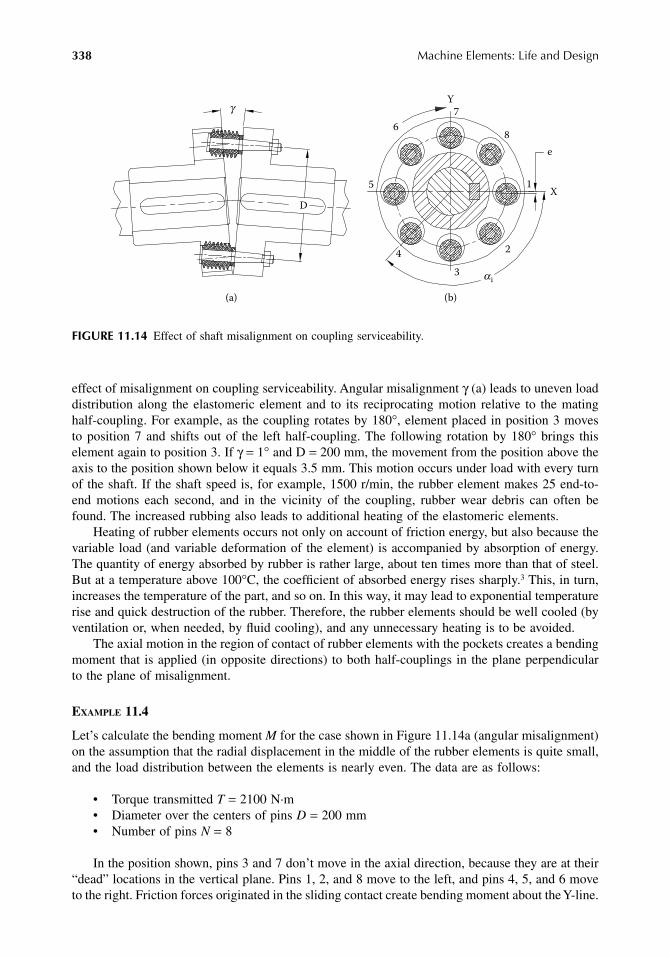
338 Machine Elements: Life and Design
effect of misalignment on coupling serviceability. Angular misalignment γ (a) leads to uneven loaddistribution along the elastomeric element and to its reciprocating motion relative to the matinghalf-coupling. For example, as the coupling rotates by 180°, element placed in position 3 movesto position 7 and shifts out of the left half-coupling. The following rotation by 180° brings thiselement again to position 3. If γ = 1° and D = 200 mm, the movement from the position above theaxis to the position shown below it equals 3.5 mm. This motion occurs under load with every turnof the shaft. If the shaft speed is, for example, 1500 r/min, the rubber element makes 25 end-to-end motions each second, and in the vicinity of the coupling, rubber wear debris can often befound. The increased rubbing also leads to additional heating of the elastomeric elements.
Heating of rubber elements occurs not only on account of friction energy, but also because thevariable load (and variable deformation of the element) is accompanied by absorption of energy.The quantity of energy absorbed by rubber is rather large, about ten times more than that of steel.But at a temperature above 100°C, the coefficient of absorbed energy rises sharply.3 This, in turn,increases the temperature of the part, and so on. In this way, it may lead to exponential temperaturerise and quick destruction of the rubber. Therefore, the rubber elements should be well cooled (byventilation or, when needed, by fluid cooling), and any unnecessary heating is to be avoided.
The axial motion in the region of contact of rubber elements with the pockets creates a bendingmoment that is applied (in opposite directions) to both half-couplings in the plane perpendicularto the plane of misalignment.
EXAMPLE 11.4
Let’s calculate the bending moment M for the case shown in Figure 11.14a (angular misalignment)on the assumption that the radial displacement in the middle of the rubber elements is quite small,and the load distribution between the elements is nearly even. The data are as follows:
• Torque transmitted T = 2100 N·m• Diameter over the centers of pins D = 200 mm• Number of pins N = 8
In the position shown, pins 3 and 7 don’t move in the axial direction, because they are at their“dead” locations in the vertical plane. Pins 1, 2, and 8 move to the left, and pins 4, 5, and 6 moveto the right. Friction forces originated in the sliding contact create bending moment about the Y-line.
FIGURE 11.14 Effect of shaft misalignment on coupling serviceability.
8
7
1
2
3
4
5
6
(a) (b)
e
Y
X
D
g
ai
9563_C011.fm Page 338 Wednesday, July 25, 2007 4:37 PM

Connection of Units 339
The average load of one pin equals
The bending moment equals the sum of friction force moments about the Y-line:
In position turned by 22.5°, the bending moment M is a bit greater:
In this calculation, the friction coefficient f = 0.5. It is worth greasing the rubber elements andpockets to decrease the f value. It is also important to decrease the angular misalignment. If it issmall, the axial movement of the resilient elements can be kept within the ability of the rubber todeform elastically. The sliding will be prevented and the bending moment will be decreased.
Figure 11.14b shows the effect of radial misalignment e. If the rubber elements are driving androtating in the arrow direction, then element 1 is the most loaded, and element 5 transmits thelowest load (if at all). This uneven load distribution between the elements brings about a lot ofimperfections in the behavior of the machine, as shown in the following list:
The service life of the rubber elements decreases, because all of them (in turn) pass throughthe overloaded zone during one revolution of the shaft.
Because the vector sum of the forces in the coupling doesn’t equal zero, the shafts becomeloaded with a radial force. This force results in an additional bending moment applied toboth shafts and additional loads, both radial and axial, applied to their bearings. The vectorof the coupling force has the same direction as the radial offset of the shafts, thus the bendingmoment is of constant direction, and the rotating shafts are exposed to cyclic bending.
The axial force is created when the radial misalignment is combined with angular misalignmentin a perpendicular plane. This effect is similar to that discussed in Section 6.2.3 regardingthe misaligned cylindrical roller bearings.
The unavoidable results of coupling misalignment are increased vibration and noise.
All the imperfections mentioned in the preceding list can occur not only due to misalignment, butalso because of differences in dimensions and hardness of the elastomeric elements within onecoupling. Errors in half-coupling geometry are possible as well. In these cases, the additional radialforce rotates with the shaft and increases the vibrations by far. In one way or another, couplingsalways create some additional forces that can be larger or smaller depending on the quality andstiffness of the coupling and, mainly, on the alignment of the shafts.
EXAMPLE 11.5
Calculate the additional radial force F for the case presented in Figure 11.14b. The data are asfollows:
Torque transmitted T = 2100 N·mDiameter over the pin centers D = 200 mm
FT
D NNa = = ⋅
⋅=2 2 2100
0 2 82625
.
M F fD
a i= ⋅ = ⋅ ⋅ +Σ2
2625 0 50 22
2 0 4 45cos ..
( cos cosα ++ = ⋅2 90 634cos ) N m
M N m= ⋅ ⋅ + = ⋅2625 0 50 22
4 22 5 4 67 5 686..
( cos . sin . )
9563_C011.fm Page 339 Wednesday, July 25, 2007 4:37 PM
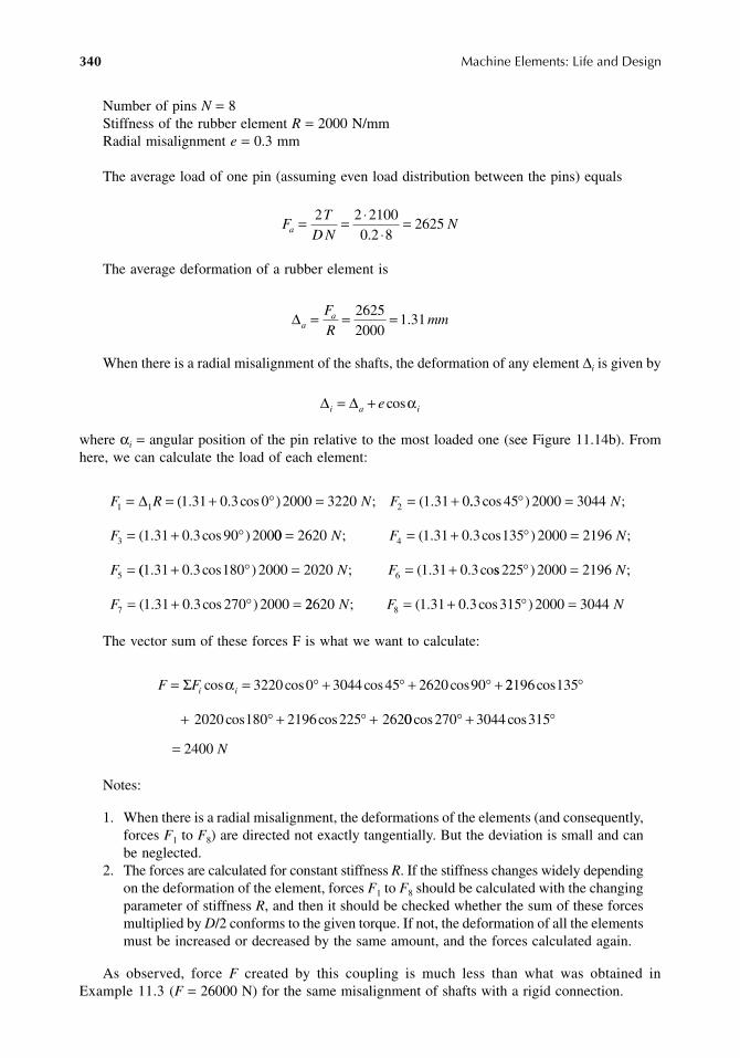
340 Machine Elements: Life and Design
Number of pins N = 8Stiffness of the rubber element R = 2000 N/mmRadial misalignment e = 0.3 mm
The average load of one pin (assuming even load distribution between the pins) equals
The average deformation of a rubber element is
When there is a radial misalignment of the shafts, the deformation of any element ∆i is given by
where αi = angular position of the pin relative to the most loaded one (see Figure 11.14b). Fromhere, we can calculate the load of each element:
The vector sum of these forces F is what we want to calculate:
Notes:
1. When there is a radial misalignment, the deformations of the elements (and consequently,forces F1 to F8) are directed not exactly tangentially. But the deviation is small and canbe neglected.
2. The forces are calculated for constant stiffness R. If the stiffness changes widely dependingon the deformation of the element, forces F1 to F8 should be calculated with the changingparameter of stiffness R, and then it should be checked whether the sum of these forcesmultiplied by D/2 conforms to the given torque. If not, the deformation of all the elementsmust be increased or decreased by the same amount, and the forces calculated again.
As observed, force F created by this coupling is much less than what was obtained inExample 11.3 (F = 26000 N) for the same misalignment of shafts with a rigid connection.
FT
D NNa = = ⋅
⋅=2 2 2100
0 2 82625
.
∆aaF
Rmm= = =2625
20001 31.
∆ ∆i a ie= + cos α
F R N F1 1 21 31 0 3 0 2000 3220 1 31 0= = + = = +∆ ( ). . cos ; ( . .. cos ) ;
( . . cos )
3 45 2000 3044
1 31 0 3 90 2003
=
= +
N
F 00 2620 1 31 0 3 135 2000 21964
5
= = + =
=
N F N
F
; ( . . cos ) ;
(( . . cos ) ; ( . . co1 31 0 3 180 2000 2020 1 31 0 36+ = = + N F ss ) ;
( . . cos )
225 2000 2196
1 31 0 3 270 20007
=
= + =
N
F 22620 1 31 0 3 315 2000 30448N F N; ( . . cos )= + =
F Fi i= = + + +Σ cos cos cos cosα 3220 0 3044 45 2620 90 22196 135
2020 180 2196 225 262
cos
cos cos
+ + + 00 270 3044 315
2400
cos cos +
= N
9563_C011.fm Page 340 Wednesday, July 25, 2007 4:37 PM

Connection of Units 341
Figure 11.15 shows couplings in which the elastomeric element is loaded in shear. In versiona, rubber part 1 is glued or vulcanized to steel parts 2 and 3. This coupling is so designed that theshear stress is constant throughout the volume of the rubber part. It is achieved by placing coincidentvertices of cones on the shaft axis (point C in Figure 11.15a).
If the last statement is not obvious, it can be easily proved. As is known, the dependencebetween shear stress τ and strain is as follows (see Figure 11.16a):
FIGURE 11.15 Flexible couplings with elastomeric elements loaded in shear.
FIGURE 11.16 Shear stress distribution in a twisted rubber element.
C
1 23 4
6
5
(a) (b)
τ γ= =Gtl
G
t
l
l
dr
r
Ri
RO
(a)
ga
(b)
9563_C011.fm Page 341 Wednesday, July 25, 2007 4:37 PM

342 Machine Elements: Life and Design
For the rubber element, designed as shown, the following correlations are valid:
Here, ϕ is the angle of twist, which is obviously the same for all sections and layers of therubber element. So are the angle α and the modulus of elasticity in shear G.
The infinitesimal torque created by the shear stress τ is given by
From here, the torque equals
From this equation, the shear stress can be obtained:
The admissible shear stress is about 0.2–0.3 MPa.4
Figure 11.15b shows a coupling with toroidal tirelike elastomeric element 4 connected to thesteel half-couplings by means of backing rings 5. The latter rings are made of two halves each (forassembly reasons) and united through the medium of rings 6. This coupling is the most flexibleamong those shown here, that is, the admissible amounts of misalignment are bigger than that ofany other resilient coupling. But its dimensions are relatively large. Besides, at higher speeds, thiscoupling creates axial forces directed inward. This behavior should be taken into consideration.
Couplings shown in Figure 11.15 have a common drawback: if the rubber (or the attachmentof the rubber to half-coupling) fails, the machines suddenly disconnect. In some cases, this can beunacceptable.
11.2.4 GEAR COUPLINGS
Resilient couplings have larger dimensions because the load capacity of elastomeric elements israther limited. In addition, they are also flexible in torsion (their torsion angles can be as large as3° or 4°). Therefore in many cases, mechanical couplings are used, which are made mainly ofsurface-hardened steels, have relatively small dimensions and weight, and provide the neededcompensation for shaft misalignment due to movable connections inside them. One of the mostwidespread couplings of this kind is the gear coupling (Figure 11.17). It consists of two toothedhubs 1 and 2 and a connecting part (sleeve) with internal toothing. The sleeve can be made of twohalves (3 and 4) connected by bolts or as an integral part 5 with end covers 6. These couplings arelubricated with oil that is filled in or emptied through plug 7 or with grease. Seals 8 and O-ringsin the flange connections prevent oil leakage from the coupling.
t r l r
r
rG G const
= =
= = =
ϕ α
τ ϕα
ϕα
; tan ;
tan tan
22
22
22
dT r dr r r dr= ⋅ ⋅ ⋅ = ⋅τ π τ π2 2 2
T dT r dr R RR
R
R
R
i
i i
= = = −( )∫ ∫0 0
223
203 3π τ π τ
τπ
=−( )
3
2 03 3
T
R Ri
9563_C011.fm Page 342 Wednesday, July 25, 2007 4:37 PM

Connection of Units 343
Power loss in gear couplings is about 0.25–0.65% at straight teeth and 0.10–0.25% at crownedteeth.5 Therefore, at low and medium speed, the convective heat transfer suffices for cooling. Butwhen the coupling transmits high power, oil flow through the teeth is usually needed to take upthe heat. The oil is poured inside the coupling, and the parts are so designed that centrifugal forcespush the oil through the mesh. To enable effective oil flow, the clearances in the mesh should bebig enough.
Sleeve 1 (Figure 11.18a) is centered in the toothed connections relative to the hubs and can’tmove in the radial direction. Therefore, between the hub and the sleeve there can only be angularmisalignment. The shafts’ misalignment is compensated in the gear coupling by the pivot of thesleeve around the hub toothing, as if these connections are spherical or universal joints. But theyare not, and so the ability of gear couplings to compensate for misalignment is rather limited.
Angle γ can be either the same for both connections (when the shafts are parallel, Figure 11.18a)or different (γ1 and γ2 in Figure 11.18b). Thus, these angles should be calculated separately for
FIGURE 11.17 Gear coupling.
FIGURE 11.18 Gear coupling misalignment.
8
3 4
1 2
6
57
γ1 γ2
(a) (b)
1
γ γ
e
L
9563_C011.fm Page 343 Wednesday, July 25, 2007 4:37 PM
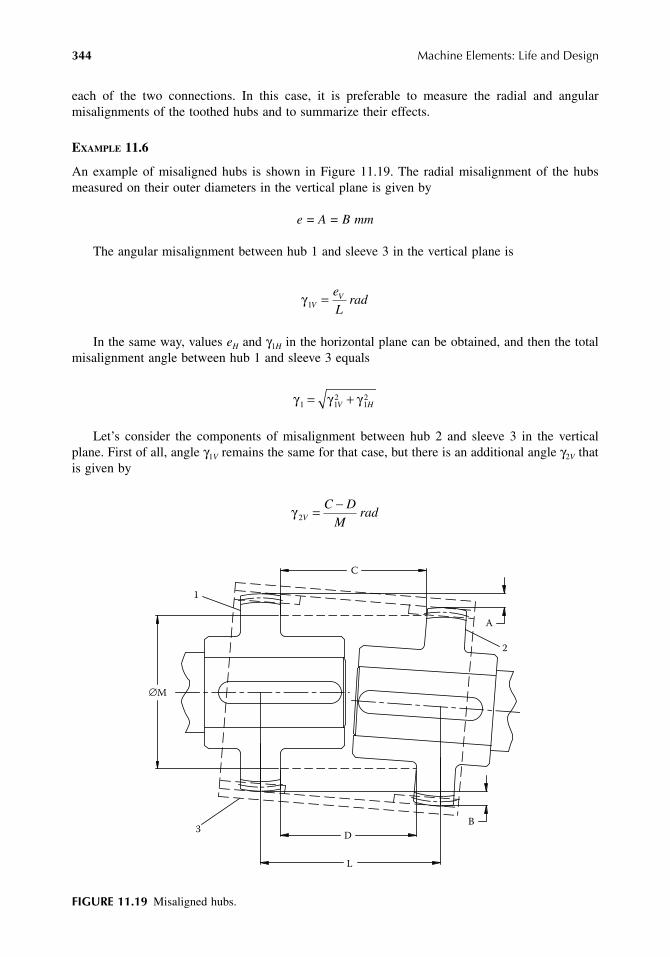
344 Machine Elements: Life and Design
each of the two connections. In this case, it is preferable to measure the radial and angularmisalignments of the toothed hubs and to summarize their effects.
EXAMPLE 11.6
An example of misaligned hubs is shown in Figure 11.19. The radial misalignment of the hubsmeasured on their outer diameters in the vertical plane is given by
e = A = B mm
The angular misalignment between hub 1 and sleeve 3 in the vertical plane is
In the same way, values eH and γ1H in the horizontal plane can be obtained, and then the totalmisalignment angle between hub 1 and sleeve 3 equals
Let’s consider the components of misalignment between hub 2 and sleeve 3 in the verticalplane. First of all, angle γ1V remains the same for that case, but there is an additional angle γ2V thatis given by
FIGURE 11.19 Misaligned hubs.
γ 1VVe
Lrad=
γ γ γ1 12
12= +V H
γ 2V
C DM
rad= −
1
2
3
∅M
C
A
B
L
D
9563_C011.fm Page 344 Wednesday, July 25, 2007 4:37 PM

Connection of Units 345
where M is the diameter at which the C and D dimensions are measured.The combined misalignment angle in the vertical plane is given by
In the case represented in Figure 11.19, the “minus” sign must be chosen, because both γ1V
and γ2V are turned in the same direction. (It is obvious that if γ1V = γ2V, γ2VC = 0. This is the casewith hub 2.) In Figure 11.18a, where the axes of the hubs are parallel, the misalignments betweenthe hubs and the sleeve are equal. If one of the hubs had been turned around the center of itstoothing by angle γ clockwise, its misalignment relative to sleeve 1 would have been decreased tozero with no effect on the misalignment of another hub.
In the same way, the combined misalignment γ2HC in the horizontal plane can be obtained, andthen the total misalignment between hub 2 and the sleeve equals
Figure 11.20a shows the position of the hub teeth relative to the internal teeth of the sleevewhen they are turned with respect to each other by angle γ. As was said, hub 1 and sleeve 2 arecentered relative to each other, either by the working surfaces of the involute teeth or by the outerdiameter of the toothing. The last case is typical for high-speed applications, where exact centering
FIGURE 11.20 Angular misalignment and the shape of crowned teeth.
γ γ γ2 1 2VC V V= ±
γ γ γ2 22
22= +VC HC
1
Rt
2
3
4
5
3
A
6
7
(a) (b)
F1
F2
tS
γ
b
γ
S
∆
W
γ
90°
γ
9563_C011.fm Page 345 Wednesday, July 25, 2007 4:37 PM

346 Machine Elements: Life and Design
is needed to limit imbalance. The radial clearance in this case is very small (0.02–0.04 mm), andthe top surface of the hub teeth should have the shape of a sphere to enable the unimpeded turnof the hub. But this is not enough. Let’s take note of tooth 3 of the hub that lies in the spacebetween teeth 4 and 5 of the sleeve. This is the very place where the ability of the connectionmembers to turn relative to each other is geometrically limited. If the teeth of both the hub andthe sleeve are straight and the backlash is zero, no free turning is possible in this connection. Thebigger the backlash, the bigger (in direct proportion) the possible turning angle, but if straight,the teeth would contact their edges. To improve the contact of teeth, they are usually made crownedas shown in Figure 11.20. The technology of cutting such teeth is very simple in principle, butquite complicated in realization. When cutting straight teeth, the gear-cutting tool (hob) movesstraight in the feed direction, (Figure 11.21a). To cut the crowned teeth, the hob moves throughan arc as shown in Figure 11.21b. For that purpose, the hobbing machine must be equipped withan additional mechanism that provides the needed feed motion of the hob. Once this feature isadded, this machine can be used for cutting hubs with crowned teeth with different barreling.
To calculate the needed barreling, let’s return to Figure 11.20b where the section of the crownedtooth 3 is drawn in a bigger scale, so that we can make some geometric calculations. The curvedprofile of tooth 3 is characterized by radius Rt, and it is so built that it is tangent to the straightprofile of the sleeve’s tooth 4 at the point of contact A. From the geometrical construction, we canobtain the radius of the barreled tooth profile:
(11.7)
If the tooth thickness in the middle equals S, on the ends, it is S – 2∆, where
(11.8)
The nominal tooth space tS of the sleeve needed to place tooth 3 is also obtained from thegeometric calculations:
(11.9)
FIGURE 11.21 Hobbing of straight and crowned teeth.
RW
t =2sin γ
∆ = −Rt ( cos )1 γ
t S WS = − +( )cos sin2 ∆ γ γ
(a) (b)
RH
RP
W
d
Toothed
hub
Feed
motion Feed
motionHob
9563_C011.fm Page 346 Wednesday, July 25, 2007 4:37 PM

Connection of Units 347
Now we are to define the contour of hob feed motion. Figure 11.22 shows the relation betweenthe radial motion of the hob and the thickness of the cut tooth. When the hob is moved toward thework by δ (from position 1 to 2), the cut tooth becomes thinner by 2∆, where
(11.10)
Here, ϕ = pressure angle (usually ϕ = 20°).From the geometry shown in Figure 11.21b, we obtain (after simple transformations) the path
radius of the hob pitch line:
(11.11)
To calculate radius RH, the pitch radius of the hob should be added to RP.
EXAMPLE 11.7
Given data: gear coupling m = 5 mm, addendum height = 0.8m, pressure angle ϕ = 20°, teethnumber N = 40, face width of the hub toothing W = 40 mm, and misalignment angle γ = 3°. Thesleeve is centered by the outer diameter of the teeth.
From Equation 11.7 and Equation 11.8,
This means that the tooth on the ends is thinner by 1.048 mm than in the middle. The nominaltooth thickness on the pitch circle equals (in standard case) 0.5πm. Let’s take the same thicknessfor the first approximation:
FIGURE 11.22 Relationship between hob radial motion and tooth thickness.
3
2
1
∆
δ
ϕ
∆ = ⋅δ ϕtan
RW W
P = + ≈2 2
8 2 8δδ
δ
R mm
mm
t = =
= − =
40
2 3382
382 1 3 0 524
sin
( cos ) .
∆
S mm= ⋅ ⋅ =0 5 5 7 854. .π
9563_C011.fm Page 347 Wednesday, July 25, 2007 4:37 PM

348 Machine Elements: Life and Design
The space width of the sleeve obtained from Equation 11.9 is given by
Now is the time to evaluate this result. The nominal width of the sleeve tooth space on thepitch circle equals 0.5πm = 7.854 mm. To place the turned tooth, we have to increase the width to8.890 mm. This means that the internal tooth of the sleeve becomes thinner by about 1 mm, thatis, 6.818 mm instead of 7.854 mm. Is that OK? If we don’t like this result, we can make the hubtooth thinner (by decreasing the S value) and thereby make the sleeve tooth thicker. But possiblyit is OK, and the calculation of the teeth for the bending strength can only give the right answer.
To continue: The values of S and tS have been calculated for zero backlash. But the backlashis needed to enable the oil to flow through the teeth also in position, where the teeth have themaximal inclination relative to the tooth space of the mating part. In addition, the possible tem-perature difference between the hub and the sleeve and the geometrical errors of the teeth must betaken into account to prevent jamming of the coupling. We will decrease the hub tooth thicknessby around 0.1m = 0.5 mm, i.e., S = 7.35 mm. Now all the dimensions of the hub and sleeve teethcan be calculated.
The δ value (see Equation 11.10) is
Then the path radius of the hob pitch line (from Equation 11.11) is given by
In the case shown in Figure 11.20, the end point of contact is placed on the end of the tooth.To avoid that, the tooth length can be just enlarged from W to Wt (see Figure 11.23) with no changeto the values calculated in the preceding text.
When the hub and sleeve are misaligned, tooth 3 (Figure 11.20) and its diametrically placedfellow sufferer are the most loaded, whereas teeth 6 and 7 are the least loaded. Figure 11.24 showsthe change in clearances between the hub and the sleeve teeth over 90° (between tooth 3 and 6 inFigure 11.20). Here we can see that the teeth in the upper part of the picture are just idle.
FIGURE 11.23 Enlarged tooth length.
t mmS = − ⋅ + ⋅ =( . . ) cos sin .7 854 2 0 524 3 40 3 8 890
δϕ
= = =∆tan
.tan
.0 524
201 44
°mm
R mmP =⋅
=408 1 44
1392
.
W
Wt
9563_C011.fm Page 348 Wednesday, July 25, 2007 4:37 PM
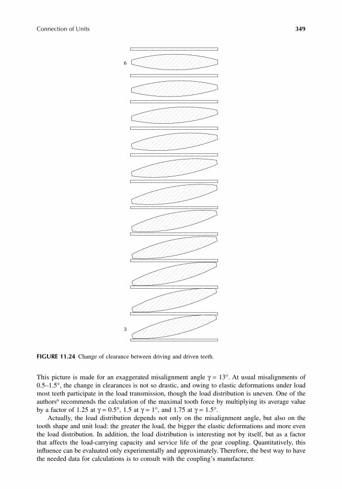
Connection of Units 349
This picture is made for an exaggerated misalignment angle γ = 13°. At usual misalignments of0.5–1.5°, the change in clearances is not so drastic, and owing to elastic deformations under loadmost teeth participate in the load transmission, though the load distribution is uneven. One of theauthors6 recommends the calculation of the maximal tooth force by multiplying its average valueby a factor of 1.25 at γ = 0.5°, 1.5 at γ = 1°, and 1.75 at γ = 1.5°.
Actually, the load distribution depends not only on the misalignment angle, but also on thetooth shape and unit load: the greater the load, the bigger the elastic deformations and more eventhe load distribution. In addition, the load distribution is interesting not by itself, but as a factorthat affects the load-carrying capacity and service life of the gear coupling. Quantitatively, thisinfluence can be evaluated only experimentally and approximately. Therefore, the best way to havethe needed data for calculations is to consult with the coupling’s manufacturer.
FIGURE 11.24 Change of clearance between driving and driven teeth.
3
6
9563_C011.fm Page 349 Wednesday, July 25, 2007 4:37 PM

350 Machine Elements: Life and Design
As is seen from Figure 11.20, each tooth (during one revolution) moves from position 6 toposition 7 and then returns to position 6. This means that each tooth performs reciprocal slidingmotion relative to the mating teeth of the sleeve, and the friction forces produce a bending momentapplied to both of the meshing parts in the plane perpendicular to the plane of misalignment. Themechanism of this effect is the same as in the resilient coupling with pins and rubber sleeves(discussed in the preceding text). The magnitude of the bending moment depends on the coefficientof friction f and the load distribution between the teeth. If the misalignment angle is so great thatthe entire load is transmitted by tooth 3 (Figure 11.20) and its diametrically opposite twin, thebending moment is maximal and is given by
(11.12)
whereT = torque transmittedd = pitch diameter of the teethϕ = pressure angle on the pitch diameter (usually ϕ = 20°)f = coefficient of friction (for common applications, f = 0.10–0.205)
The minimal magnitude of bending moment takes place when the load is distributed evenly betweenthe teeth. The infinitesimal friction force dFf applied to small element r · dα (see Figure 11.25) is asfollows:
The infinitesimal bending moment
FIGURE 11.25 Computation of bending moment in a gear coupling.
MT f
dd T f
max cos cos= ⋅
⋅⋅ = ⋅22ϕ ϕ
dFT f
r rr d
T fr
df = ⋅⋅
⋅ = ⋅cos cosϕ π
απ ϕ
α2 2
dM dF hT fr
d rT f
df= ⋅ = ⋅ ⋅ = ⋅ ⋅2 2π ϕ
α απ ϕ
αcos
sincos
sin αα
αhdα
r = d/2
9563_C011.fm Page 350 Wednesday, July 25, 2007 4:37 PM
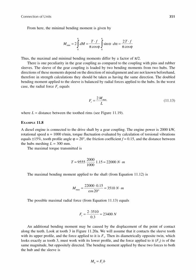
Connection of Units 351
From here, the minimal bending moment is given by
Thus, the maximal and minimal bending moments differ by a factor of π/2.There is one peculiarity in the gear coupling as compared to the coupling with pins and rubber
sleeves. The sleeve of the gear coupling is loaded by two bending moments from two hubs. Thedirections of these moments depend on the direction of misalignment and are not known beforehand,therefore in strength calculations they should be taken as having the same direction. The doubledbending moment applied to the sleeve is balanced by radial forces applied to the hubs. In the worstcase, the radial force Fr equals
(11.13)
where L = distance between the toothed rims (see Figure 11.19).
EXAMPLE 11.8
A diesel engine is connected to the drive shaft by a gear coupling. The engine power is 2000 kW,rotational speed n = 1000 r/min, torque fluctuation evaluated by calculation of torsional vibrationsequals ±15%, tooth profile angle ϕ = 20°, the friction coefficient f = 0.15, and the distance betweenthe hubs meshing L = 300 mm.
The maximal torque transmitted is
The maximal bending moment applied to the shaft (from Equation 11.12) is
The possible maximal radial force (from Equation 11.13) equals
An additional bending moment may be caused by the displacement of the point of contactalong the teeth. Look at tooth 3 in Figure 11.20a. We will assume that it contacts the sleeve toothwith its upper profile, and the force applied to it is F1. Then its diametrically opposite twin, whichlooks exactly as tooth 3, must work with its lower profile, and the force applied to it (F2) is of thesame magnitude, but oppositely directed. The bending moment applied by these two forces to boththe hub and the sleeve is
M dMT f
dT f
min cossin
cos= = ⋅ ⋅ = ⋅∫ ∫2
2
0 0
π π
π ϕα α
π ϕ
FM
Lr = 2 max
T N m= = ⋅955520001000
1 15 22000.
M N mmax
.cos
= ⋅ = ⋅22000 0 1520
3510°
F Nr = ⋅ =2 35100 3
23400.
M F bb = 1
9563_C011.fm Page 351 Wednesday, July 25, 2007 4:37 PM

352 Machine Elements: Life and Design
Provided that the misalignment angle is so great that the entire torque is transmitted by twoteeth under consideration, the following relations are valid:
Here γ is the misalignment angle in rad.This bending moment acts in the plane of misalignment and may be of remarkable magnitude
at a large misalignment. When the misalignment is small, the load is distributed more evenly overthe circumference, and the b value is small so that this moment can be neglected.
Another peculiarity of gear couplings with crowned teeth is that they don’t like working atzero misalignment. If the misalignment is zero or very small, the contact patch (hatched, seeFigure 11.26) remains immovable or moves only slightly, so that most of the contact area remainsconstantly compressed with no access for the lubricant. Combined with high pressure andmicromovements, this creates suitable conditions for fretting (see also Chapter 2). Moderatemisalignment, which brings about sliding motion in the teeth contact, enables renewal of the oilfilm on the contact surfaces and also facilitates creation of a hydrodynamic oil wedge.Experiments7 have shown that the gear coupling with a certain radius of the crowned tooth profilehas an optimal misalignment angle, at which the friction coefficient f is minimal. At greatermisalignment, the f value rises because of growing unevenness of load distribution and slidingvelocity. At smaller misalignment, the f value rises because of worsening of the lubricationconditions in the contact regions.
REFERENCES
1. Roark, R.J. and Young, W.C., Formulas for Stress and Strain, McGraw-Hill Kogakusha.2. Timoshenko, S., Strength of Materials. Part II, D. Van Nostrand Company, Princeton, NJ.3. Poturaev, V.N. and Dirda, V.I., Rubber Elements of Machines, Mashinostroenie, Moscow, 1977
(in Russian).
FIGURE 11.26 Contact patch on a crowned tooth.
F FTd
b R R
MT
dR
t t
b t
1 2 2 2
2
= = = ≈
=
; sin ;
,max
γ γ
γ
9563_C011.fm Page 352 Wednesday, July 25, 2007 4:37 PM

Connection of Units 353
4. Poljakov, V.S., Barbash, I.D., and Rjakhovsky, O.A., Couplings Handbook, Leningrad, Mashinostroenie,1974 (in Russian).
5. Popov, A.P., Gear Couplings in Seaborne Machinery, Sudostroenie, Leningrad, 1985 (in Russian).6. Reshetov, D.N., Machine Elements, Mashinostroenie, Moscow, 1989 (in Russian).7. Handbuch der Schadenverhütung, Herausgabe von der Allianz Versicherungs AG, Berlin, 1976
(in German).
9563_C011.fm Page 353 Wednesday, July 25, 2007 4:37 PM

9563_C011.fm Page 354 Wednesday, July 25, 2007 4:37 PM

Part III
Life Prediction of Machine Parts
Calculations for strength are incorporated into almost all phases of the development process of amechanism. During preliminary specifications, when the designs diagram is to be chosen, itsfeasibility must be proven by strength calculations. Here, approximate calculations are mostly used,such as estimation of shaft diameter using Equation 4.1 and Equation 4.2 or gear dimensions fromEquation 7.11. Thereupon, in the course of detailed design, the strength calculations are made indetail. When the mechanism is on trials or in service, it may fail for various reasons, and theinvestigation of the failures mostly involves additional calculations for strength and durability. Lateron, if the customer wants some upgrade of the mechanism (for example, to a greater capacity), thestrength calculations are indispensable.
Who is to make these calculations? At a design office there is usually one or a group ofengineers specializing in strength calculations. To do his work, the stress engineer must receivefrom the designer the detailed drawings of the mechanism, with all dimensions, tolerances,materials, and so on. To prepare these drawings, the designer himself has to make all the strengthcalculations needed to choose the dimensions, materials, etc. Thus, the final calculation madeby the stress engineers is verifying only, but if it reveals that the designer was mistaken and theproject must be done anew … oh, no!
In practice, the designer can consult with the stress engineer about the accepted method ofcalculation. He also can order calculation of some parts that are critically stressed or that needmore sophisticated mathematical tools or computer programs in which the designer is not an expert.But the rest, which amounts to about 90% or 100% of the strength calculations, the designer hasto do himself. So he is not able to do his job if he is not friendly with the strength calculations.
The methods of such calculations are usually taken from the technical literature, or they arerecommended by professional societies. (As an example of the latter can be mentioned Lloyd’sstandards in ship building, ASME and SAE approved calculations in automobile construction,aircraft construction, and others.) Unfortunately, the correct substitution of numbers for letters inthe equations recommended doesn’t ensure the reliable operation of the mechanism.
Once, at a plant manufacturing marine engines, a meeting was held concerning the fracture ofa crank shaft. One of the main participants in this meeting was the guru in this field, the author ofthe method of strength calculations for crank shafts. One young engineer asked him:
9563_C012.fm Page 355 Wednesday, July 25, 2007 4:39 PM

356
Machine Elements: Life and Design
“How could the crankshaft break, if the safety factor equals 5?!”“If the shaft broke, that means, there was no safety margin,” said the professor calmly, andeverybody appreciated his answer.
This distant case obviously shows that sometimes it is very difficult to develop a strengthcalculation method that takes into account quite precisely both the complicated shape of the machinepart and the intricate loading conditions, associated sometimes with unknown operation and main-tenance factors. In such cases the researcher develops an approximate method and uses it to calculatethe stresses in a number of machines of the same type that are known to be safely working. Thequotient obtained when the admissible stress of material the part is made from is divided by thestress calculated using the approximate method is defined as the safety factor. Hence, the safetyfactor is essentially an index of the lack of knowledge attached to a certain method of calculation.It is clear that in the design of a similar mechanism, such a calculation gives only the firstapproximation. Later on, the reliability of the mechanism, and possibly the real stresses, have tobe checked during trials.
Nowadays the calculation methods have improved drastically, but the real reliability and servicelife of the machine parts remains an estimate. Now, as well as in the distant past, the failure at asafety factor of 5 is sometimes possible. The authors are going to discuss in detail the basics ofcalculation for strength and durability. They also want to inspire in the reader’s mind an under-standing of some conventions and, to some extent, the uncertainty of these calculations to urge himto be cautious about the results obtained.
“The world rests on three things,” the ancient sages said. Each of them had his own version ofwhat these were. The authors, being in agreement with their subject’s requirements, can stateunequivocally that the calculation for strength is based on three data units:
• The strength parameters of the material• The stress magnitude and pattern of change with time• The safety factor
Each of these data units deserves detailed discussion.
9563_C012.fm Page 356 Wednesday, July 25, 2007 4:39 PM

357
12
Strength of Metal Parts
Strength is the ability of a material to withstand loading forces without damage. In Section 3.1,mechanisms of destruction of the crystal lattice in a metal under load have been discussed. Atpresent, the knowledge in this field is still insufficient to determine the admissible stresses fordifferent loading conditions. This purpose is reached more safely by processing experimental data.
Engineers noticed long ago that the repeated application of a moderate load may in time bringabout the failure of a part, whereas the static application of the same load doesn’t cause any visiblechange to the material. The first systematic research of what had been called “fatigue of metal”was undertaken by August Wöhler during 1857–1870. He tested until failure railroad axles loadedwith a bending moment in a rotating-beam testing machine, the plotted results yielding the first
σ
–
N
(or
S
–
N
) curves. (Here
σ
=
bending stress,
N
=
number of cycles to failure). Such a plot isshown in Figure 12.1a.
These plots are usually drawn in log-log coordinates, (see Figure 12.1b). In these coordinates,the
σ
–N curve can be plotted as a broken line. Its sloping part 1 is expressed by the equation
(12.1)
Here
m
=
1/tan
α
=
the slope angle. The greater the
m
is, the less the slope of the line and thestronger the dependence of the number of cycles to failure on the stress magnitude. For smoothparts, the
m
value may differ from 4 to 10, and for parts with stress raisers (the vast majority aresuch) from 4 to 6.
1
Another source
2
recommends taking the
m
value as approximately 13.6 forsmooth shafts and 9.3 for notched shafts. As we see, the stress raisers (also known as stress
risers
or stress
concentrations
) decrease the
m
value. It is also known that stronger materials have greater
m
values. To consider these two factors, the following formula has been offered:
7
where
C
=
some constant coefficient (
C
=
12–15 for carbon steels, and
C
=
20–35 for alloy steels)
K
=
factor of fatigue strength decrease that integrates the harming influences of the stress raiser, surface properties, and size factor
If, for example, the stress concentration factor
K
t
=
2, surface factor
K
S
=
0.9, and size factor
K
d
=
0.9, then
K
=
2/(0.9 · 0.9)
=
2.47, and for an alloy steel
m
=
8–14. We can see that the
m
value is very undependable.The horizontal part 2 of the
σ
–
N
curve corresponds to the maximal stress of the repeated loadcycle S
lim
that doesn’t lead to a failure at an infinite number of cycles. This value is often referredto as the “fatigue strength” or “fatigue limit.”
At a relatively short life span (up to 10
4
cycles) portion 1 of the
σ
–
N
curve gives an inflatedstrength estimate, and so the
σ
–
N
curve in this area is represented more truly by portion 3. Herethe metal undergoes significant plastic deformations, and the admissible stress amplitude must becalculated using the strain–life method (see Section 12.1.3). This case is rare in machinery.
N Cons tm⋅ =σ tan
mCK
=
9563_C012.fm Page 357 Wednesday, July 25, 2007 4:39 PM

358
Machine Elements: Life and Design
The number of cycles
N
0
to the breakpoint of the
σ
–
N
curve lies in the range 10
6
–3 · 10
6
.Therefore endurance tests usually last 5 · 10
6
–10
7
cycles: if the specimen doesn’t fail within thisperiod, it will not fail at this stress magnitude at all.
Occasionally, the failure may occur after 10
7
cycles as well, because fatigue failure is essentiallyprobabilistic. But it doesn’t influence appreciably the accepted
S
lim
magnitude because the occa-sional exception occurs too infrequently to be statistically significant.
The
σ
–
N
plot shown in Figure 12.1b is typical for steels of low and middle strength. High-strength alloy steels and light alloys don’t have the horizontal part of the
σ
–
N
curve; that is, theadmissible stress magnitude decreases continuously with the increase in number of load cycles(Figure 12.1c). Nevertheless, the breakpoint of the
σ
–
N
curve at
N
0
cycles remains. Exponent
m
is approximately 10 times greater at portion 4 than at portion 1.
1
Let’s see the effect of the stress on the service life before and after the breakpoint. Let’s assumethat at portion 1,
m
1
=
10,
N
0
=
10
6
cycles and the stress
σ
1
=
1.1
S
lim
. From Equation 12.1,
Let’s see now what happens at portion 4 of the
σ
–
N
curve, where
m
3
=
100, provided that
σ
3
=
0.9
S
lim
:
FIGURE 12.1
The
σ
–
N
curves.
N
σ
log NN0
N0 log N
log σ
log σ
(a) (b)
(c)
Slim
Slim
1 2
1 4
σi
Ni
Su
3
3Sstat
Slim
α
N S N
N NS
010
1 110
1 01
10
6101
1
⋅ = ⋅
=
= ⋅
lim
lim
σ
σ ...
10 39 10
10
6
= ⋅ cycles
N S N
N NS
0100
3 3100
3 03
100
610
⋅ = ⋅
=
=
lim
lim
σ
σ11
0 93 76 10
100
10
..
= ⋅ cycles
9563_C012.fm Page 358 Wednesday, July 25, 2007 4:39 PM

Strength of Metal Parts
359
So we see that the increase of stress by 10% above S
lim
has led to decrease of durability by afactor of 2.6, whereas the decrease of stress by 10% below S
lim
has increased the durability by afactor of 3760. Thus, the breakpoint parameters (
S
lim
and
N
0
) are very important also in a case inwhich the material has no infinite life stress.
By the way, is 3.76 · 10
10
cycles a lot or not? For example, the crankshaft of a car engine makesin the mean about 2000 r/min. During 30 years of work 6 h daily the crankshaft makes 7.9 · 10
9
turns. Because of the four-stroke engine, the combustion stroke takes place once in two turns ofthe crankshaft, so the number of cycles with high bending stress equals 3.95 · 10
9
only.Almost all machines perform cyclic work, and their parts are exposed to a load that changes
in conformance with a certain program. Therefore, calculation for fatigue strength has becomethe dominant method. Nevertheless, against the background of repeated load cycles, an accidentaloverload with a very small number of cycles may occur. The admissible stress in this case ishigher than at a high-cycle load, and it is most often set equal to the stress that is bearable understatic load.
12.1 STRENGTH OF METALS
12.1.1 S
TRENGTH
AT
A
S
TATIC
L
OAD
For static strength calculations, we use the mechanical properties of materials that are specified instandards, the manufacturers catalogs, or in reference books. In important cases, the supplierprovides the results of the test for static strength along with the material.
The most used strength characteristics are the ultimate strength
S
u
(also called
tensilestrength
), yield point
S
y
, and hardness. Among the required data are the parameters of plasticity(tensile strain
δ
and necking
ψ
, both taken at the fracture point of the specimen) and impacttoughness (determined by the Charpy V-Notch test). These parameters are always paid attentionto: The steel for engineering purposes must not be brittle. It is desirable to have
δ
≥
6%, ψ ≥10%, and the impact toughness not less than 50 J/cm2. At the same time, these three parametersdon’t appear in the strength calculation. That indicates that we lack knowledge in this field.
The mechanical properties of metals change with temperature: as the temperature increases,the strength of a metal reduces, and the plasticity increases. The strength parameters obtained atroom temperature are valid up to approximately 300°C for steels and 100–150°C for light metals.For higher temperatures, the possible decrease in mechanical properties and creep resistance shouldbe considered.
At low temperatures, the strength of a metal increases (the change is not big and usually is nottaken into consideration), but the plasticity decreases considerably, and at a certain low temperaturecalled the transition temperature, it falls sharply, making the metal brittle similar to glass. (Thecurious observer is encouraged to research maritime shipping disasters.) Normally, structural steelscan be used safely up to −20°C. When the temperature lowers to −40°C, the impact toughness ofthe material, as well as the starting conditions of the mechanism, should be checked. For example,if a combustion engine must be warmed up before starting, the real working temperatures can bemuch higher than that of the environment.
At −60°C, we usually use alloy steels that retain satisfactory impact toughness at this temper-ature. Among the specified strength parameters for steels intended for use at low temperatures mustbe the impact toughness at these temperatures.
The mechanical properties of metals are obtained by tensile test of specimens that have standarddimensions to get comparable results from different tests. Typical design of a specimen is shownin Figure 12.2a (d = 5–10 mm). The specimen is loaded in tension until failure on a special testingmachine that is able to plot the deformation of the specimen vs. the tension force. The failedspecimen is shown in Figure 12.2b, and two types of force-deformation plots are given in Figure 12.3.
9563_C012.fm Page 359 Wednesday, July 25, 2007 4:39 PM

360 Machine Elements: Life and Design
The tensile strength Su and yield point Sy are obtained by dividing the respective forces by thenominal section areas of the specimen:
Here P1 (or P2) = maximal force at which the plastic deformation of the material reaches some
conventional value (mostly 0.2%)Pmax,1 (or Pmax,2) = maximal tension force registered during the test
A0 = area of the nominal cross section of the specimen
FIGURE 12.2 Typical tensile test specimen.
FIGURE 12.3 Stress–strain diagram.
(a)
(b)
NeckL
L0
d
SPA
SP
A
SPA
SP
y u
y u
, ,max,
, ,max,
;
;
11
01
1
0
22
02
= =
= = 22
0A
Strain
Ten
sio
n f
orc
e
P1
P2
Pmax,2
Pmax,1
9563_C012.fm Page 360 Wednesday, July 25, 2007 4:39 PM

Strength of Metal Parts 361
In the course of the test, the specimen elongates (elastically and plastically), and its diameterdecreases because the volume of metal remains nearly constant. But the decrease in the cross-sectional area is relatively small (at least until necking that takes place after the force Pmax has beenreached). Therefore, the Sy and Su values are usually calculated as if the cross section remainsunchanged.
The tensile strain δ is obtained from the formula
where dimensions L0 and L are the length of the specimen before and after the test (Figure 12.2).Because the elongation of the specimen is largely accounted for by the necking, the δ value dependson the length of the specimen. For steels, at L0 = 5d it is greater than at L0 = 10d by 22%.3
Materials have complicated structure, and the random orientation of crystals in grains and ofgrains relative to their neighbors cause certain scatter of mechanical properties, even if the speci-mens are cut from one blank. The strength can fluctuate depending on the following factors:
• Real chemical composition of the heat and its cleanliness• Forging reduction ratio• Location in the forging or casting the specimen is cut from• Direction of the specimen axis: along the grain flow or across• Peculiarities of the heat treatment procedure, location of the part in the furnace, and so on
For most machine elements, the stress must not exceed the yield point because plastic deforma-tion leads to changes in their geometry. For this reason, the stress admissible at static loading isobtained by division of the yield stress by some safety factor that considers the possible uncertaintiesin the stress estimation (see chapter 13). But sometimes, when some small change in the geometryof the part is admissible, plastic deformation is acceptable and can be useful. Besides the casesdescribed in Chapter 3, Section 3.3, screw connections can be mentioned. Though the plasticdeformation in the root of the thread coil occurs at a relatively small load, it decreases neither thestatic strength, nor the fatigue strength of the bolt. This deformation increases the strength of material(strain hardening) and induces residual stresses directed opposite to the working stresses.
Tensile tests are very fast and relatively cheap. But they require the tensile-test machine andspecimens made of the same material with the same heat treatment as the part to be calculated forstrength. Much cheaper is the hardness test that in many cases can be performed directly on thepart with no damage to its quality. Therefore, it is useful to apply the dependence between theBrinell or Rockwell hardness and the strength parameters of steels shown in Figure 12.4. Thesediagrams must be considered as approximate, though.
We have spoken so far about one-dimensional loading (tension–compression). The real stateof stress can be more complicated. The material can be loaded simultaneously with normal andshear stresses or with normal stresses only but in two mutually perpendicular directions (biaxialstress). The yield stress in such cases can be determined from equations by Tresca orHüber–Mises–Hencky. The latter theory is based on strain energy and conforms closely to theexperimentally observed effects associated with the beginning and development of yield in metals.For a multiaxial stress, when there are all the possible components of stress, the yield criterionlooks as follows:
(12.2)
δ = −L L
L0
0
100 %
σ σ σ σ σ σ σ τ τeq x y x z y z xy xz= − + − + − + +1
262 2 2 2 2( ) ( ) ( ) ++( )
=τ yz yS2
1 2/
9563_C012.fm Page 361 Wednesday, July 25, 2007 4:39 PM

362 Machine Elements: Life and Design
whereσeq = equivalent stressσx, σy, σz = main normal stressesτxy, τxz, τyz = main shear stresses
If only one normal (σ) component and one shear (τ) stress component are applied to the material(for example, bending and torsion of a round bar), Equation 12.2 for equivalent stress takes the form
(12.3)
and the condition of the beginning of yield,
(12.4)
From this condition follow the relations for special cases:
• For pure tension (τ = 0), the yield begins at
σ = Sy
• For pure torsion (σ = 0), the yield begins at
(12.5)
where Sy,τ = yield point in shear.
FIGURE 12.4 Approximate dependence on hardness of the steel mechanical properties.
Carbon steel
Alloy st
eel
Brinell hardness
180200
200
300
400
220 240 260 280
Str
ess,
MP
a
600
500
700
800
900
300 320
S–1
Su
1000
1100
Sy
σ σ τeq = +( ) /2 2 1 23
( ) /σ τ2 2 1 23+ = Sy
3 0 577τ τ τ= = =S S Sy y y; .,
9563_C012.fm Page 362 Wednesday, July 25, 2007 4:39 PM

Strength of Metal Parts 363
Equation 12.5, which connects the yield points in tension and in shear, conforms to theexperimental data.
From Equation 12.5 we have the following:
Substituting this into Equation 12.4 instead of the factor 3, we have
(12.6)
This is the condition for the onset of yield. If we want to prevent yielding, we have to insert somesafety factor n. Let’s introduce the idea of a partial safety factor (separately for the normal andshear stresses):
In this case, Equation 12.6 becomes:
To have the overall safety factor n, the following condition should be fulfilled:
or, similarly,
(12.7)
12.1.2 FATIGUE STRENGTH (STRESS METHOD)
The modes of failure at a repeated load and the number of cycles to failure depend on the stressmagnitude. At a stress that is close to the tensile strength, the specimen deforms plastically andthe number of cycles is very small. At lower stresses, when the cycles to failure number 102–104,there can be found both plastic deformation and an array of fatigue cracks. This mode of failureis called low-cycle fatigue (LCF), and in this case the life of the part should be calculated by thestrain method (see Subsection 12.1.3). Decreasing the stress further decreases the plastic deforma-tion. When the number of cycles to failure exceeds 105, the specimens fail in fatigue, with no
S
Sy
y
2
23
,τ
=
σ τ
σ τ
τ
τ
22
22 2
2
2
2
21
+
=
+ =
S
SS
S S
y
yy
y y
,
,
nS
nSy y
σ ττ
σ τ= =; ,
1 11
2 2n nσ τ
+ =
1 1 12 2 2n n nσ τ
+ =
nn n
n n=
+σ τ
σ τ2 2
9563_C012.fm Page 363 Wednesday, July 25, 2007 4:39 PM

364 Machine Elements: Life and Design
visible plastic deformation, and the life prediction is usually made by the stress method (discussedin this section).
The LCF condition in machinery occurs rarely. For example, a shaft rotating with a speed of1000 r/min makes 105 turns in less than 2 h. So in the vast majority of practical cases, the numberof cycles exceeds N0, and we have to check the parts for high-cycle fatigue (HCF) or for infiniteservice life.
The process of failure in HCF is much more complicated than that in static loading. It ischaracterized by the following features:
• Initiation and development of a crack happens without any visible deformation of thepart. As a rule, there are no changes in the operation of the machine, until the crackextends over the majority of the cross section and brings about catastrophic failure.
• Onset of the initial crack, its propagation, and failure of the part occur at stresses muchlower than the yield stress.
• The fatigue crack starts mostly from surface blemishes, such as surface asperities(roughness), nicks (caused by negligent storage and handling), corrosion, marking andstamping of all kinds (impact, chemical, or electrographic), marks of hardness tests(Rockwell, Brinell, or Vickers), fretting (see Chapter 2), etc.
• Another kind of common crack initiation place is the necessary fillets, keyways, grooves,splines, and other features that concentrate and focus the stresses just as the aforemen-tioned accidental stress raisers do.
As was said, fatigue cracks mostly start from the surface of a part; therefore, the surfacecondition has a great effect on the results of the fatigue test. The surface of the specimen can beturned on a lathe, ground, polished (by hand, mechanically, or electrically). In all these cases, thecondition of the surface layer and the residual stresses in it can be very different, depending notonly on the kind, but also on the parameters of the machining process, and they can hardly becontrolled. Because of this, the scatter of experimental points in fatigue tests is much greater thanfor tensile tests, and the determination of fatigue characteristics of a metal (such as fatigue limit)needs quite a lot of experiments to obtain reliable data.
The load fluctuation in time can be of different kinds. Figure 12.5 shows several typical cases:
1. Shear stress in the propeller shaft of a ship2. Bending stress in the root of a gear tooth3. Bending stress in the root of an idler pinion tooth4. Bending stress in a rotating shaft bent by a moment of constant direction
Because the loading options are countless, it is common practice to test the specimens in fatigueunder sinusoidal load. The admissible stresses obtained in these tests are then used for loadingcycles different from the sinusoidal. So the sinusoidal diagrams shown in Figure 12.6a, Figure 12.6b,and Figure 12.6d can be substituted for the real loading diagrams represented in Figure 12.5a toFigure 12.5d.
It is convenient to represent the loading diagram as a sum of two components: mean stressσm (such as a static load) and harmonic component with the amplitude σa (see Figure 12.6). Itis convenient because tests have shown that the damaging effect of mean stress is much lessthan that of the harmonic component (of course, only if the maximal stress σmax doesn’t reachthe yield point). Therefore, it is conventional to determine the admissible stress amplitude ofa certain loading cycle as admissible amplitude of a pure harmonic component (also calledsymmetric cycle; see Figure 12.6d) with the addition of some part of the mean stress (see thefollowing text).
9563_C012.fm Page 364 Wednesday, July 25, 2007 4:39 PM

Strength of Metal Parts 365
To label the loading diagrams with respect to proportion between σa and σm, parameter R wascoined:
If σa = 0, R = 1 (static load). If σa = σm, R = 0 (pulsating cycle; see Figure 12.6b). If σm = 0,R = −1 (symmetric cycle; see Figure 12.6d). The limiting stresses Slim for the cycles characterizedby R = 0 and R = −1 are designated as S0 and S−1, respectively. The vast majority of fatigue testsare made with the symmetric loading cycle (σm = 0) realized in rotating bending. (See Figure 12.7;the bending deformation here is highly exaggerated.) So the S−1 value called the fatigue limit (orendurance limit) became the main parameter that rates the fatigue strength of material. In real
FIGURE 12.5 Examples of stress variation with time.
Str
ess
Time0
0
(a)
Time
(b)
Time
(c)
Time
(d)
0
0
Str
ess
Str
ess
Str
ess
R m a
m a
a
m
a
m
= = −+
=−
+
σσ
σ σσ σ
σσσσ
min
max
1
1
9563_C012.fm Page 365 Wednesday, July 25, 2007 4:39 PM

366 Machine Elements: Life and Design
machines may happen load conditions with different R values, and the limiting stress amplitude ofthe harmonic component Sa is determined from the equation
where f(σm) is some function that accounts for the effect of mean stress. The function is still amatter of discussion at the time of printing this book.
The effect of the mean stress σm on the limiting value of the alternating stress has been studiedexperimentally. If the set of specimens is tested with a constant σm and stepwise-decreased σa, wefinally receive (in coordinates σa − σm) a point that conforms to infinite life at this very σm value.A set of such tests with different magnitudes of σm gives several points, and we can draw a line
FIGURE 12.6 Mean stress, amplitude, and maximal and minimal stress of a cycle.
FIGURE 12.7 Rotating–bending endurance test machine.
Stress
Time0
0
0
0
(a) (c)
(d)
(e)
(b)
σm
σmax
σaσmax
σm
0σa σmax
σa
σmin
σm = 0
σmin
σa
σm
σmin
σmax
σm
σa
S S fa m= −−1 ( )σ
Weight
Specimen
Weight Motor
Coupling
9563_C012.fm Page 366 Wednesday, July 25, 2007 4:39 PM

Strength of Metal Parts 367
through these points. This is a boundary line (1 in Figure 12.8), and all the combinations of σa andσm above this line conform to the sloping portion of the σ − N curve (1 in Figure 12.1), whereasall the points on line 1 conform to Slim at different σm.
Although line 1 passes through most of the experimental points, it is not as certain as a lineon paper. As was said, the results of fatigue tests have noticeable scattering, and the averaged linecan be passed through the experimental points in several ways. Therefore, there are several sim-plifying suggestions about the boundary line equation, and the simplest is the Goodman diagram.It is a straight line (2 in Figure 12.8) that connects two well-known points: S−1 on the vertical axis(when σm = 0, i.e., symmetric cycle) and Su on the horizontal axis (when σa = 0, i.e., static load).
Let’s designate Sa and Sm, the vertical and horizontal coordinates of any point B, on line 2. Inthis case, the equation of line 2 is
(12.8)
or, similarly,
(12.9)
Because the maximal stress must not exceed the yield point Sy , additional constraint line 3 isplotted; its equation is
FIGURE 12.8 Goodman’s diagram of the fatigue limit vs. the mean stress.
S–1
Sy
2 (Goodman line)
3 (yield line)
Sa
σa
Mean stress σm
4
D
A
C
B
6
1
5
Sy SuSmσm
Har
mo
nic
str
ess
amp
litu
de
σ a
45°
S SS
Sam
u
= −
−1 1
S
S
S
Sa m
u−
+ =1
1
σ σm a yS+ =
9563_C012.fm Page 367 Wednesday, July 25, 2007 4:39 PM

368 Machine Elements: Life and Design
Thus, the sought-for limiting combinations of σa and σm are placed on the hatched sections oflines 2 and 3. But in the subsequent equations, line 3 doesn’t play a part; it is just taken to meanthat σmax must not exceed Sy.
The admissible combination of σa and σm (point A in Figure 12.8) is less than the limitingcombination of Sa and Sm because there should be a certain factor of safety. Let’s calculate thesafety factor for three different cases, reasoning from the Goodman diagram:
1. Where σa and σm are changing in the same proportion: For example, in a gear, when thetorque transmitted grows, the tooth forces and bending moments applied to the shaftgrow in the same proportion.
2. Where σm remains constant, but σa changes: The propeller shaft of a ship can be takenas an example. The mean shear stress at a given rotational speed is constant. The alternatingshear stress is caused by torsional vibration, nonuniform fluid flow field, and other factors.
3. Where σmin = σm − σa = constant: This case belongs to bolted connections, where theminimal load equals the preload force and remains constant.
In the first case, the σa/σm ratio remains constant; therefore, the limiting point B is placed online 4 (because all points of this line have the same ratio σa/σm). The equation of line 2:
(12.10)
The equation of line 4:
Point B of intersection of lines 2 and 4 has the vertical coordinate
Hence, the safety factor for the first case is
(12.11)
In the second case, the limiting point C lies on line 5 because all points on this line have thesame σm value. The equation of line 5 is
Substituting this in Equation 12.10, we obtain the vertical coordinate of point C:
ySS
x Su
= − +−−
11
y xa
m
= σσ
SS
SS
a
u
m
a
=+ ⋅
−
−
1
11σσ
nS
S S
a
a a m
u
1
1
1= =+
−
σ σ σ
x m= σ
y S SSa
m
u
= = −
−1 1
σ
9563_C012.fm Page 368 Wednesday, July 25, 2007 4:39 PM

Strength of Metal Parts 369
From here, the safety factor for the second case is
In the third case, line 6 drawn at 45° meets the condition σm − σa = constant. The equation ofthis line is:
The vertical coordinate of limiting point D (the intersection of lines 2 and 6) is
The safety factor for the third case is
It should be pointed out that the Goodman criterion, although prevalent, has a grave disadvantage:it overestimates the influence of mean stress on the fatigue strength of the metal. Specifically, experimentswith bolts have shown1 that the limiting stress amplitude Sa remains practically constant up to Sm ≤ 0.9Sy.Among the other approximations of the experimental points, the following are mentioned.
Gerber’s suggestion (1874) — a parabolic failure criterion:
Or, in terms of Sa,
(12.12)
The ASME suggestion — an elliptic failure criterion:
Or, again in terms of Sa,
(12.13)
Both these suggestions are used only rarely.
nS S
Sa
a a
m
u2
1 1= = −
−
σ σσ
y x a m= + −σ σ
y S SS
S Sau a m
u
= = + −+−
−1
1
σ σ
nS S S
S Sa
a a
u a m
u3
1
1
= = + −+
−
−σ σσ σ
S
S
S
Sa m
u−
+
=1
2
1
S SS
Sam
u
= −
−1
2
1
S
S
S
Sa m
u−
+
=1
2 2
1
S SS
Sam
u
= −
−1
2
1
9563_C012.fm Page 369 Wednesday, July 25, 2007 4:39 PM

370 Machine Elements: Life and Design
In the engineering environment in Russia, the suggestion of S.V. Serensen4 is in use everywhere.According to this, the limiting curve 1 (Figure 12.9) connects three control points: S−1, S0, and Su.This diagram is plotted on the σmax − σm coordinates. Point A conforms to a pure harmonic cycle(S−1), and point B, to a pulsating cycle (S0). To simplify the equations, portion A–B of curve 1 isreplaced by straight line 2, and then
(12.14)
where
Substitution of Smax = Sa + Sm into Equation 12.14 gives
(12.15)
A similar equation is valid for the shear stresses:
(12.16)
For specimens without stress raisers the following values of ψσ and ψτ have been experimentallyfound: for carbon steels ψσ = 0.1–0.2, ψτ = 0–0.1; and for alloy steels and light alloys ψσ =0.15–0.30, ψτ = 0.05–0.15.
FIGURE 12.9 Serensen’s diagram of maximal stress vs. mean stress.
Sy
1
2
σmax
σm
A
B
S–1
Su
Sa
3
S0
0.5 S0 SuSySm
Sa
45°
S S Smmax ( )= + −−1 1 ψ σ
ψ σ = −−2 1 0
0
S S
S
S S Sa m= − ⋅−1 ψ σ
τ τ ψ ττa m= − ⋅−1
9563_C012.fm Page 370 Wednesday, July 25, 2007 4:39 PM

Strength of Metal Parts 371
In all cases, the greater values should be chosen for stronger materials. If σm < 0, it isrecommended to take ψσ = ψτ = 0. The maximal stress must not exceed Sy.
EXAMPLE 12.1
Alloy steel of HB 300, Su = 1050 MPa, S−1 = 500 MPa. What is the limiting amplitude Sa, if themean stress Sm = 300 MPa?
According to Goodman (Equation 12.8),
According to Gerber (Equation 12.12),
According to ASME (Equation 12.13),
According to Serensen (Equation 12.15),
Who is right? We have already discussed the scattering of experimental data. Each of thementioned authors may appear closer to the truth than the others in some specific cases, dependingon the material properties and loading conditions. If you want to know more precisely the limitingstresses for a certain material under certain loading conditions, you have to undertake the suitabletests. Then you will know who is right. But if you don’t have such a possibility, you are forced totake chances and gain experience. The authors got accustomed to Serensen’s method in the courseof several decades and take it as reliable.
Let’s introduce the idea of equivalent stress σa,eq: This is the amplitude of a symmetric cycle,which has the same damaging effect on the material as the real loading cycle characterized bystresses σa and σm. It is clear that the safety factor n at the equivalent stress must be the same asat the real load cycle. Hence, the equivalent stress can be determined as follows:
If we take Goodman’s diagram and the first case, when the safety factor is determined byEquation 12.11, the equivalent stress
(12.17)
S MPaa = −
=500 1300
1050357
S MPaa = −
=500 1300
1050459
2
S MPaa = −
=500 1300
1050479
2
S MPaa = − =500 0 15 0 30 300 455 410( . . )
σa eq
Sn, = −1
σ σ σ σ σa eqa m
ua
umS
S SSS, = +
= +−−
−1
1
1
9563_C012.fm Page 371 Wednesday, July 25, 2007 4:39 PM

372 Machine Elements: Life and Design
The next, similar expression is valid for the shear stresses:
(12.18)
In the same way can be determined the equivalent stresses for other cases, and also for otherways of plotting the limiting lines. Specifically for Serensen’s approach,
Until now we have dealt with one-dimensional loads (tension–compression, or bending, orshear). Inasmuch as the fatigue phenomena are by nature associated with plasticity (see Section 3.1),it is assumed that Equation 12.2 to Equation 12.7 written for the static strength are valid for thefatigue strength as well. But the parameters σy and τy shall be replaced by S−1 and S−1,τ, respectively.In this case, the boundary strength equation (Equation 12.6) becomes
(12.21)
This equation implies a symmetric cycle (σm = τm = 0), in which σa and τa are the amplitudesof alternating stresses, which are synchronous and cophasal. Accordingly, Equation 12.4, whenapplied to fatigue, takes the form
(12.22)
Here we have
This relation is verified experimentally, but if it is not exactly true, factor 3 in Equation 12.22can be replaced by the stress ratio:
(12.23)
When the loading cycle is asymmetric (σm ≠ 0 and τm ≠ 0), the strength condition can be writtenby analogy with Equation 12.6:
(12.24)
(12.19)
(12.20)
τ ττ
ττa eq a
um
S,
,= + −1
σ σ ψ σ
τ τ ψ τ
σ
τ
a eq a m
a eq a m
,
,
= +
= +
σ τ
τ
a a
S S
2
12
2
12
1− −
+ =,
σ τa a S2 213+ = −
SS
−
−
=12
12
3,τ
σ ττ
a a
S
SS2
1
2
21+
=−
−−
!
,
σ τ
τ
a eq a eq
S S, ,
,− −
+
=
1
2
1
2
1
9563_C012.fm Page 372 Wednesday, July 25, 2007 4:39 PM
Strength of Metal Parts 373
Using, on the analogy of static strength, the partial safety factors
(12.25)
we obtain the equation for the safety factor in the form
or
(12.26)
In the case of compound stress with all components acting, the equivalent amplitude σ*a,eq andthe equivalent mean stress σ*m,eq should be determined first. By analogy with Equation 12.2,
The equivalent stress, which takes into account both the alternating and mean stresses, isdetermined by analogy with Equation 12.17 and Equation 12.19, written for uniaxial stress:
The safety factor is determined as before:
The drawback of such a method is in the estimation of the influence of the compressive meanstress (σm < 0). From experiments, it is known that the compressive mean stress increases theadmissible amplitude of the harmonic component. This effect is reflected in Equation 12.17 toEquation 12.20, respectively. In Equation 12.28 the mean stress σ*m,eq is positive in principle, andthis decreases the calculated safety factor (as compared with the real one) in the area of compressivemean stresses. The effort to consider more precisely the influence of the mean stresses5 is madefor the case of proportional loading, that is, when all kinds of stresses change simultaneously, andin the same proportion. Criteria for more complicated cases offered in the literature are based onSines’ criterion.
(12.27)
(12.28)
(12.29)
(12.30)
nS
nS
a eq a eqσ τ
τ
σ τ= =− −1 1
,
,
,
;
1 1 12 2 2n n nσ τ
+ =
nn n
n n=
+σ τ
σ τ2 2
σ σ σ σ σ σ σ
σ
a eq a a a a a a
m
, ( ) ( ) ( )∗ = − + − + −1
21 2
21 3
22 3
2
,, ( ) ( ) ( )eq m m m m m m∗ = − + − + −1
21 2
21 3
22 3
2σ σ σ σ σ σ
σ σ σ
σ σ ψ σσ
a eq a equ
m eq
a eq a eq m e
SS, , ,
, , ,
= +
= +
∗ − ∗
∗
1
qq∗
nS
a eq
= −1
σ ,
9563_C012.fm Page 373 Wednesday, July 25, 2007 4:39 PM

374 Machine Elements: Life and Design
We guess that Equation 12.27 to Equation 12.30 can be used as they are; although they reducethe calculated safety factor, they are not too conservative. As stated earlier, in Equation 12.15 andEquation 12.16, it was recommended to take ψσ = ψτ = 0 at σm ≤ 0. This recommendation alsodecreases the calculated safety factor, though to a lesser extent. Another example provides theGoodman limiting line (dotted line 3 in Figure 12.9), which is drawn below the experimental points.Nevertheless, the Goodman approach has found wide application in strength calculations.
It should be taken into consideration that the inaccuracy of some limiting line or equation isonly a small part of the many inaccuracies, uncertainties, and assumptions that accompany thecalculations for strength and durability.
As we could see, the main characteristic of the material needed for fatigue calculation is thefatigue limit S−1. This parameter can be determined only experimentally, but this research needsmany specimens to make the results statistically reliable. In most cases, the engineer doesn’t havethe possibility to undertake this expensive and time-consuming work, and this basic parameter isobtained approximately from empiric formulas such as the following:6
For normalized and annealed steels:
S−1 = 0.454Su+8.4 MPa
For carbon steels after quenching and tempering:
S−1 = 0.515Su – 24 MPa
For alloy steels after quenching and tempering:
S−1 = 0.383Su+94 MPa
For high-alloy austenitic steels:
S−1 = 0.484Su MPa.
When these formulas are used, the error in the S−1 value doesn’t usually exceed 15%.
12.1.3 LIMITED FATIGUE LIFE UNDER IRREGULAR LOADING (STRESS METHOD)
When the fluctuating stress exceeds the fatigue limit, the life span of the part is limited. If the stressamplitude is constant, the number of stress cycles to failure can be estimated from Equation 12.1,and the example of such a calculation has been provided earlier. But if the stress amplitude changeswith time as shown in Figure 12.10, the less-damaging effect of smaller stresses should be considered.
Line 1 in Figure 12.10 presents the change of stress amplitude in time, and line 2 shows thechange of the loading frequency (for example, this can be the rotational speed of a shaft). The loadcurve is sectioned so as to replace the curve by several stress levels. The greater the number ofsections, the closer is the bar diagram to the load curve. Each stress level σi has its own loadingfrequency and time of application, and their product gives the number of cycles ni at this stressmagnitude. Here σ1 is the maximal stress amplitude in the spectrum, and σi is any of the smalleramplitudes.
An approach to this problem was offered by A. Palmgren (1924) for ball bearings and thenadapted by M.A. Miner (1945) for aircraft structures. The idea is based on the assumption that anycyclically loaded part has some resource of resistance that is not spent when the stress is less than thefatigue limit. But when the stress is higher, the resistance resource is used up in proportion to the numberof cycles. For example, if σ1 = 600 MPa and the number of cycles to failure N1 = 3 · 105 cycles, then
9563_C012.fm Page 374 Wednesday, July 25, 2007 4:39 PM

Strength of Metal Parts 375
loading during n1 = 1 · 105 cycles takes up 33.3% of the resistance ability of the material. Ifafterward the same part is loaded, say, with σ2 = 550 MPa, then N2 = 7.2 · 105 (provided that m =10), and to use up the remaining 66.7% of the resistance ability, the duration of work under thisload should be n1 = 7.2 · 105 · 0.667 = 4.8 · 105 cycles. In other words, if we symbolize as ni thenumber of loading cycles at σi, and as Ni the number of cycles to failure at this stress, the criterionof exhaustion of the resistance resource should look as follows:
(12.31)
From the foregoing, it follows that the contribution of each loading step to the consumption ofresistance resources depends on its “damaging ability” per cycle. For example, if at σ1 = 600 MPathe number of cycles to failure N1 = 3 · 105 cycles, and at σ2 = 550 MPa, N2 = 7.2 · 105 cycles,each cycle of σ1 damages the part as much as 2.4 cycles of σ2. Hence, the cycles of lesser load canbe added to the cycles of maximal load according to their relative “damaging abilities.” So theequivalent number of cycles ne at maximal amplitude σ1 is given by
Experiments have shown that Equation 12.31 is not exact, and
where the C value may vary within the range from 0.25 to 4.7 Momentary overload stress mayreduce the C value to 0.05–0.1. For design purposes, C = 1 is usually taken, but it should be keptin mind that the real service life of the part may be ten times less than the calculated.
FIGURE 12.10 Spectrum of stresses and frequencies.
Time
Fatigue limitSR
1
2
σi
σ1
0
Str
ess
amp
litu
de
Lo
adin
g f
req
uen
cy
(str
ess
cyc
les
per
sec
on
d)
n
Ni
i∑ = 1
n n n n ne
m m
ii= +
+
+ +
1 22
13
3
1 1
σσ
σσ
σσ
+m
n
NCi
i∑ =
9563_C012.fm Page 375 Wednesday, July 25, 2007 4:39 PM

376 Machine Elements: Life and Design
EXAMPLE 12.2
The fatigue limit of material, S−1 = 500 MPa, N0 = 3 · 106 cycles. The fatigue curve exponent m = 10.The part is cycled with the following parameters of load: σa = 300 MPa during 95% of the workingtime with the frequency of f = 1000 cycles per minute (cpm); σa = 600 MPa during 3%, f = 800cpm; σa = 650 MPa during 1.5%, f = 500 cpm; and σa = 750 MPa during 0.5% of the workingtime, f = 300 cpm. The service life should be at least 100 h. Is the part strong enough?
First let’s determine the number of cycles for the stresses that exceed the fatigue limit, beginningwith the maximal stress:
σa1 = 750 MPa; n1 = 100 · 60 · 300 · 0.005 = 0.9 · 104 cyclesσa2 = 650 MPa; n2 = 100 · 60 · 500 · 0.015 = 4.5 · 104 cyclesσa3 = 600 MPa; n3 = 100 · 60 · 800 · 0.03 = 14.4 · 104 cycles
Now the equivalent number of cycles under the maximal load can be determined:
The number of cycles to failure at maximal load
According to this calculation, only 68% of the material strength resources are used up during100 h of work. If the stresses given previously have been already multiplied by an appropriatesafety factor (that means, the real stresses are not greater than the calculated ones), the result ofthis calculation can be considered as favorable.
12.1.4 FATIGUE LIFE (STRAIN METHOD)
This method was developed in the middle of the 20th century on the basis of low-cycle fatiguetests. As aforesaid, in this area the stress exceeds the yield point of the material, and the stressmethod, which doesn’t account for this effect, may give an incorrect estimate of the load capabilityof the material. Later on, the strain method was extended to include HCF as well, but in that areathe stress method, in our opinion, remains preferable. This subject is discussed in Section 12.3.
Before passing on to the basics of the strain method, we have to emphasize the differences innomenclature vs. the stress method presented earlier. These differences are historically conditioned,similar to the differences between the metric and the inch systems. Here they are:
1. In the strain method, the cyclic strain ∆ε and the cyclic stress ∆σ are meant as doubleamplitudes (ranges). Respectively, the amplitudes are εa = ∆ε/2 and σa = ∆σ/2.
2. In the strain method, N means the number of load reversals, which is twice as many asthe number of cycles. So the number of cycles equals 1/2 N.
Going to the strain method, we should recall that the phenomenon of fatigue is associated withplastic deformations in microvolumes. Among the multitude of grains forming the structure of themetal, there are grains with more imperfections in the crystal lattice (as compared to the neighbors).If this grain is so oriented that the slip plane and the shear stress are unidirectional, there occursa plastic deformation in this grain. Thus, the macrodeformation of the metal may remain elastic.
ne = ⋅ + ⋅
+ ⋅0 9 10 4 5 10650750
14 4 1060
4 4
10
4. . .00
7503 52 10
10
4
= ⋅. cycles
N NS
a
m
=
= ⋅
= ⋅−0
1
1
6
10
3 10500750
5 2 1σ
. 004 cycles
9563_C012.fm Page 376 Wednesday, July 25, 2007 4:39 PM

Strength of Metal Parts 377
At a cyclic loading, the “unlucky” grain is subjected to cyclic plastic deformation. Theamplitude of this deformation is determined not by the load applied to the very grain, but by thedeformation of the surrounding mass of the part. Because the mass works in the elastic rangeand obeys Hooke’s law, the constant amplitude of load causes constant amplitude of deformation,too. Consequently, the considered grain is subjected to plastic deformation with constant ampli-tude. The behavior of this grain is of interest for the strength calculation, because the fatiguecrack initiates in it.
Needless to say, experiments can’t be performed with a grain, but with a specimen only. It isassumed that a smooth specimen, when tested at constant amplitude of strain (elastic + plasticdeformation), is able to simulate the rupture of the metal grain under consideration. In other words,it is supposed that there is a similarity between the behaviors of the smooth specimen in theconditions of test stated previously and the microscopic volume of the real part under cyclic plasticdeformation. This concept defines the design philosophy based on the linkage between the fatiguelife of a part with an “unlucky” grain and that of the specimen cycled with the same level of stress.Accordingly, the expected fatigue life (until the time of formation of a microcrack) can be deter-mined to sufficient accuracy when the history of deformation of the part and the strain-life fatigueproperties of the specimen are known.
The nomenclature of data for cyclically deformable materials, construction of mathematicalmodels, and test methods are widely represented in standards and special literature. The followingdefinitions are used to form the basic relations.
In Section 12.1 (Figure 12.1 and Figure 12.2) it was stated that the yield point Sy and theultimate strength Su are obtained by dividing the respective tension forces by the cross-sectionalarea of the specimen A0 before tension. Such stresses and σ–N (also known as S–N) diagrams(see Figure 3.9 [Chapter 3] and curve 1 in Figure 12.11) are used with the term “engineering”(engineering stress, engineering stress–strain curve and so on). Being hurt a bit by the shade ofneglect with respect to engineers, we have to agree that the “engineering” (in other words,approximate) approach is not valid indeed for the strain method. Because the cross section ofthe specimen reduces with the increase of the tension force, the true stress σ will be obtainedby dividing the tension force P at a given moment by the cross-sectional area A at the very samemoment of time:
FIGURE 12.11 Engineering (1) and true (2) stress–strain diagrams.
σ = PA
Strain
Str
ess
1
2
9563_C012.fm Page 377 Wednesday, July 25, 2007 4:39 PM

378 Machine Elements: Life and Design
Similarly, the idea of true deformation is introduced; it is based on the ratio of the “running”(i.e., instantaneous) elongation of the specimen to its running length:
(12.32)
From here, we derive the relation between the true deformation ε and the engineeringdeformation e:
(12.33)
These relations are valid only before necking. After necking, the elongation becomes nonuni-form over the length of the specimen. Fortunately, in practice no necking can occur, otherwise itwould be one-cycle breakage and not low-cycle fatigue.
To link the true and engineering magnitudes of stress, let’s assume that the volume of thespecimen doesn’t change during loading:
Then, taking into account Equation 12.32 and Equation 12.33, we have
(12.34)
The connection between the true stress σ and the engineering stress S is clear from the followingdefinition:
(12.35)
Because, from Equation 12.34, A0/A = 1 + e, we obtain from Equation 12.35
The total true strain consists of two components, elastic and plastic:
The elastic component is determined by Hooke’s law and is given by
(12.36)
where E = modulus of elasticity.
ε = =∫ dll
ll
l
l
00
ln
ε = +ln( )1 e
A l Al0 0 =
ε = = = +ln ln ln( )ll
A
Ae
0
0 1
σ = SA
A0
σ = +S e( )1
ε ε εt e p= +
ε σe E
=
9563_C012.fm Page 378 Wednesday, July 25, 2007 4:39 PM
Strength of Metal Parts 379
The plastic component is given in the form
(12.37)
whereK = strength coefficientn = strain hardening exponent
So the total deformation of the specimen is given by the Ramberg–Osgood equation:
(12.38)
All variables here have been determined. This relation for monotonic loading is presented graph-ically by curve 2 in Figure 12.11.
By monotonic is meant a loading with a gradually increasing force, as in a standard tensiletest. The opposite of monotonic is cyclic loading.
To find the K value, in Equation 12.37 should be substituted the true fracture stress σf and truefracture strain εf, which are determined as follows:
wherePf = breakage forceAf = cross-sectional area after breakage
where RA = reduction in the cross-sectional area, which is given by
From Equation 12.37,
Now let’s have a short break from the tedious formulas and go to some speculations about thecyclic elastoplastic deformation. In this case, the structure of dependence between stress and strainis similar to that for monotonic loading. But the members are different, because the dependence σ − εat cyclic loading is different. This relation is obtained for each material by testing a set of specimens
ε σp
n
K=
1/
ε σ σt
n
E K= +
1/
σ ff
f
P
A=
ε ff
A
A RA= =
−ln ln0 1
1
RAA A
Af=
−0
0
Kpn
f
fn
= =σε
σε
9563_C012.fm Page 379 Wednesday, July 25, 2007 4:39 PM

380 Machine Elements: Life and Design
made of this material. Each specimen is cycled with its fixed amplitude of deformation, and thetest lasts until the hysteresis loop stabilizes.
In the beginning of the cycling with a constant strain amplitude (called transition period), thestress in the metal may gradually increase (cyclic hardening, Figure 12.12a) or decrease (cyclicsoftening, Figure 12.12b), remain stable (Figure 12.12c), or even combine different modes. Theseeffects are associated with the behavior of dislocations in the crystal lattice. Usually, soft materialswith low dislocation density (such as aluminum alloys) show a tendency to cyclic hardening, andhard materials (for example, steels) are inclined to softening.
The transition period is short; then the hysteresis loop stabilizes, and, in this state, the effectseen is taken as the result of the experiment at a given amplitude of cyclic deformation.
A set of stabilized hysteresis loops obtained at different amplitudes of deformation is plottedon the same chart σ – ε as shown in Figure 12.13. Line 1 connecting the extreme points of theloops represents the dependence σ – ε at the cyclic deformation. This line is quite close to curve2 in Figure 12.11, which represents the σ – ε dependence at monotonic loading, and it is charac-terized with similar specific parameters that belong to cyclic loading. These parameters are providedwith the sign (known as a prime):
σ′y = cyclic yield strengthK′ = cyclic strength coefficientn′ = cyclic strain hardening exponent
FIGURE 12.12 Hysteresis loops in the transition period of cyclic deformation.
Strain
Str
ess
Str
ess
Time
(a)
(b)
(c)
Str
ess
Time
Str
ess
Strain
Str
ess
Time
Str
ess
Strain
9563_C012.fm Page 380 Wednesday, July 25, 2007 4:39 PM

Strength of Metal Parts 381
The cyclic yield strength is determined from the σ – ε diagram as a stress at 0.2% of plasticdeformation.
Figure 12.14 shows different variants of the correlation between the σ – ε curves for monotonousand cyclic loading: cyclic softening (Figure 12.14a), cyclic hardening (Figure 12.14b), cyclicallystable (Figure 12.14c), and mixed behavior (Figure 12.14d). Usually, metals with higher values ofthe monotonic strain-hardening exponent (n > 0.2) cyclically harden, and metals with n < 0.1cyclically soften. One more rule of thumb: the material will harden if Su/Sy > 1.4, and it will softenif Su/Sy < 1.2. In the range from Su/Sy = 1.2 to 1.4, the material may behave in any manner shownin Figure 12.14.
The total deformation, as in the case of monotonic loading, consists of elastic and plasticcomponents:
(12.39)
This is the equation of curve 1 in Figure 12.13. Equation 12.39 and Equation 12.38 are similar,because both the monotonic and the cyclic deformations are of the common nature. It is generallyagreed that in cyclic loading the dependence between amplitudes of stress and deformation (σa andεa) is defined by the same curve 1 (Figure 12.13). Based on this assumption, this dependence lookssimilar to Equation 12.39:
(12.40)
These dependences assume that the material behaves symmetrically with respect to tension andcompression. This assumption is true for homogenous materials.
FIGURE 12.13 Construction of the cyclic stress–strain curve.
Strain
Stress
1
ε ε ε σ σ= + = +′
′
e p
n
E K
1/
ε ε ε σ σa a e a p
a a
n
E K= + = +
′
′
, ,
/1
9563_C012.fm Page 381 Wednesday, July 25, 2007 4:39 PM

382 Machine Elements: Life and Design
Because εa = ∆ε/2 and σa = ∆σ/2 (see previous text), Equation 12.40 can be written in the form
(12.41)
This basic equation is widely used to describe the behavior of stresses and deformations atvarying amplitudes of loading.
Coming to the technique of numerical estimate of the fatigue life, we should recall Basquin’sformula (1910), which was chronologically the first:
(12.42)
Here∆σ/2 = true stress amplitudeσ′f = fatigue strength coefficientb = fatigue strength exponent2Nf = number of stress reversals to failure (1 reversal = 1/2 cycle)
Parameters σ′f and b define the fatigue properties of the material. To sufficient accuracy, thefatigue strength coefficient σ′f equals the true fracture stress σf. Fatigue strength exponent b is tobe determined from the steady-state hysteresis loop; usually, it ranges from −0.05 to −0.12. Virtually,
FIGURE 12.14 Differences between monotonic (1) and cyclic (2) stress–strain curves.
Str
ess
Str
ess
Strain
Str
ess
Str
ess
(a)
Strain
(b)
Strain
(c)
Strain
(d)
2
1
21
2
11, 2
∆ ∆ ∆ε σ σ2 2 2
1
= +′
′
E K
n/
∆σ σ2
2= ′f fbN( )
9563_C012.fm Page 382 Wednesday, July 25, 2007 4:39 PM

Strength of Metal Parts 383
Equation 12.42 is the same as Equation 12.1 which describes the sloping part of the Wöhler’scurve, and it belongs to the elastic portion of the strain. In log-log coordinates it is a straight line.
The next decisive step, which is made to associate the elastic and plastic components of strain,was made by Coffin and Manson. They found that the plastic strain–life data (i.e., the εp – Ndependence) can also be presented in log-log coordinates as a straight line:
(12.43)
where∆εp /2 = plastic strain amplitude2Nf = number of reversals to failureε′f = fatigue ductility coefficientc = fatigue ductility exponent
Parameters ε′f and c belong to the fracture properties of the material; ε′f approximately equalsthe true fracture ductility εf and ranges from 0.5 to 0.7.
Equation 12.43 is very important because it enables bringing together all the assumptions madepreviously. Now, from Equation 12.42 and Equation 12.43, the relation between the total strain ofa cycle and the number of cycles to failure can be written as follows:
(12.44)
The two terms of the second member of Equation 12.43 can be represented in log-log coordi-nates as two straight lines (Figure 12.15). Line 1 corresponds to the first term (elastic component ofdeformation), and line 2, to the second term (plastic component). Line 3 conforms to Equation 12.44.It is seen that at large strain amplitudes (and small numbers of stress reversals), line 3 approachesasymptotically to the line of plastic deformations that make the main contribution to the failure.At small amplitudes, elastic line 1 only determines the number of cycles to failure.
Point A is called the transition point, and shows the number of stress reversals, 2Nt, at whichthe influences of the elastic and plastic deformations are equal. The condition of their equality isobtained from Equation 12.44:
(12.45)
FIGURE 12.15 Strain–life curves: elastic (1), plastic (2), and summary (3).
∆εεp
f fN c2
2= ′ ( )
∆ ∆ ∆ε ε ε σε
2 2 22 2= + =
′+ ′e p f
fb
f fEN N c( ) ( )
2
1
NE
tf
f
b c
=′
′
−ε
σ
/( )
α
β
3
1
A
2
log 2Nf log 2Nt
log
ε′ f
9563_C012.fm Page 383 Wednesday, July 25, 2007 4:39 PM

384 Machine Elements: Life and Design
In all, the fatigue properties of metals are determined by four parameters: ε′f, σ′f, b, and c. Forcertain materials and heat treatment conditions, these factors are given in handbooks and standards,for example, SAE J1099. But many materials are not covered by the database, therefore someempirical relations that express the strain–life properties of the material through its monotonicproperties (such as Brinell hardness HB, tensile strength Su, and modulus of elasticity E) have beendeveloped. For practical use, the following relations are recommended:8
• Equation 12.44 can be approximated (suggested by Muralidharan and Manson) as follows:
(12.46)
• The fatigue strength coefficient:
• The fatigue ductility coefficient:
(12.49)
• The fatigue strength exponent b varies from −0.057 to −0.140, and on average b = −0.09.• The fatigue ductility exponent c ranges from −0.39 to −1.04, and on average c = −0.60.
This value is usually taken for metals with pronounced yield (εf ≈ 1). For high-strengthsteels (εf ≈ 0.5), c = −0.5 is most acceptable.
• The transition fatigue life (2Nt, see Equation 12.45) can be obtained from the formula:
(12.50)
The last equation, together with Equation 12.45 and Equation 12.47 to Equation 12.49, maybe useful for more exact estimation of factors b and c.
Factor b defines the slope angle of line 1 in Figure 12.15 (b = tan α), and it is clear that thecalculated durability of the part is influenced very strongly by this factor in the area of high-cyclefatigue. Substituting in Equation 12.42, b = −0.06 and b = −0.14, we obtain:
That means that the inaccurate estimation of the b value may lead to great change in the calculateddurability.
In the area of low-cycle fatigue, line 2 is the determining element, and factor c characterizes theslope angle (c = tan β). From Equation 12.43, if c = −0.6 or c = −0.5, the number of cycles to failure
(12.47)
(12.48)
∆ε ε2
0 623 2 0 01960 832
0 09=
+ ⋅−. ( ) ..
.S
ENu
f f00 155
0 53
0 562.
.
.( )S
ENu
f
−
−
′ = +
′ = +
σ
σ
f
f u
HB MPa
S MPa
4 25 225
1 04 345
. ;
.
′ = − +ε f
HB HBE
0 32 487 1910002. ( )
2 105 755 0 0071NtHB= −. .
22
16 7 7 1
N ff=
′
÷σ
σ∆
. .
22
1 67 2 0
N ff
p
=′
÷εε∆
. .
9563_C012.fm Page 384 Wednesday, July 25, 2007 4:39 PM

Strength of Metal Parts 385
Hence, in this area the variation of the c value leads to a relatively small change in the calculateddurability.
The relations obtained till now were valid for a symmetric cycle (σm = 0). For asymmetric cycles,the influence of the mean stress is taken into account on the basis of the following experimentalinformation:
1. The influence of the mean stress is substantial mainly in high-cycle fatigue. Compressivemean stress increases the fatigue life, and tension mean stress decreases it.
2. In the area of low-cycle fatigue, in which the plastic deformation becomes significant,the mean stress relaxes virtually to zero.
It is appropriate to explain here that in the macrovolume, the mean stress can’t disappear,because it is caused by the load diagram: if the load cycle has a mean load, there must be also themean stress in the loaded part. But in this case, we are considering a microvolume (or a grain) ofthe part that is subjected to elastoplastic deformation with a constant amplitude. The plasticdeformation in this microvolume relaxes the mean stress during the first cycles of loading, andonly the harmonic part of the stress remains in the sequel.
In conformity with the aforesaid, only the elastic component (the first term of Equation 12.44)shall be adapted to the mean stress:
(12.51)
This relation (suggested by Morrow) is valid for σm > 0 only. For negative mean stress, whichgives a certain positive effect, a more conservative approach is accepted, namely, σm = 0.
Now we go to multiaxial stress. Application of yield criteria (for example, Tresca or von Mises)is useful also in this case. By von Mises, the equivalent stress expressed in terms of main stresses
Let’s explore how to go to the strain–life curve for cyclic torsion, when the data for cyclictension–compression are known. By analogy with Equation 12.44, the equation for torsion looksas follows:
(12.52)
It is assumed that factors b and c remain the same. Then, taking into account the relationbetween the normal and shear stresses and deformations, Equation 12.52 is transformed to thefollowing:
(12.53)
The conversion of the stresses is made on the basis of Equation 12.5. The conversion of thedeformations is based on the expression for the equivalent deformation:
(12.54)
∆ε σ σε
22 2=
′ −+ ′f m
fb
f fc
EN N( ) ( )
σ σ σ σ σ σ σe = − + − + −1
21 2
22 3
21 3
2 1 2[( ) ( ) ( ) ] /
∆γ τγ
22 2=
′+ ′f
fb
f fc
GN N( ) ( )
∆γ σε
2 32 3 2=
′+ ′f
fb
f fc
GN N( ) ( )
ε ε ε ε ε ε εe = − + − + −23 1 2
22 3
21 3
2 1 2[( ) ( ) ( ) ] /
9563_C012.fm Page 385 Wednesday, July 25, 2007 4:39 PM

386 Machine Elements: Life and Design
In this expression is used the fact that for completely plastic deformation, Poisson’s coefficientν = 0.5; that is, the material is assumed to be incompressible. Because in torsion ε1 = −ε3 = γ/2,and ε2 = 0, the equivalent deformation is
If, instead of von Mises, Tresca’s criterion is used
Then, for pure torsion
Because at pure torsion τe = τ, we obtain (assuming that the same relation is valid for thefatigue characteristics):
(12.55)
The deformation should be determined considering that besides the elongation ε1, there is alsotransverse contraction −νε1. The equivalent shear stress is given by
But in the case of pure shear γe = γ; therefore, on the same assumption as mentioned previously,
(12.56)
Insertion of Equation 12.55, Equation 12.56, and ν = 0.5 into Equation 12.52 gives
(12.57)
These two examples with von Mises’ criteria (Equation 12.53) and Tresca’s criteria (Equation 12.57)show that the choice of criteria changes the obtained equation of the strain–life curve. But thedifferences in results remain within the usual accuracy of such calculations.
12.2 STRENGTH OF MACHINE ELEMENTS
The strength characteristics of materials are obtained from experiments with relatively smallspecimens. The strength of the real parts is sometimes also checked experimentally, but thisundertaking is time consuming; besides, the results are valid only for these parts and can hardly
ε γe =
3
τ σ σe = −1 3
2
τ σe = 1
2
′ =′
τσ
ff
2
γ ε νε ν εe
2 21
21 1
1= − − = +( ) ( )
′= + ′
γ ν εff2
12
∆γ σε
2 22 1 5 2=
′+ ′f
fb
f fc
GN N( ) . ( )
9563_C012.fm Page 386 Wednesday, July 25, 2007 4:39 PM

Strength of Metal Parts 387
be used for other parts. Therefore, in the overwhelming majority of engineering applications, fatiguestrength is calculated starting with the material properties and taking into account the differencesbetween the specimen and the part. The following differences are usually considered.
12.2.1 SURFACE FINISH
The smoother the surface, the higher is the fatigue limit. It is well known from experiments thatsurface asperities and chemical injuries facilitate the initiation of fatigue cracks. Because standardspecimens are fine-polished or mirror-polished, the surface factor for them KS = 1. The influenceof surface finish increases with increased strength of the material. As the tensile strength of steelSu rises from 400 MPa to 1400 MPa, the KS value decreases almost linearly from 0.95 to 0.85 forgrinding, from 0.92 to 0.76 for fine turning, from 0.9 to 0.6 for coarse turning, and from 0.8 to 0.3for unmachined surfaces (as forged).7
These values of KS are approximate, and in the literature can be found different recommenda-tions. But it is clear that the strength of a part can be decreased by 50% or even more because ofjust a scratch or a rust stain in the highly loaded area. The areas critical for fatigue strength are inmany cases mirror-polished and protected from harming influences, whatever their nature is.
12.2.2 DIMENSIONS OF THE PART
It has been noticed that the bigger the part, the lesser is the admissible stress amplitude. This effectis usually attributed to several factors:
• Lesser stress gradient in larger parts (Figure 12.16). As Figure 12.16 shows, at the samedepth from the surface, the part with a larger diameter has a higher stress than does thesmaller part. The more stressed subsurface layer in the larger part enhances crackpropagation from the surface into the interior. (It should be mentioned that the fatiguelimit in tension, where the stress gradient is zero, is less than in bending by about15–20%.6)
• Inferior quality of the metal achievable in larger parts due to metallurgical problems(nonuniformity of mechanical properties over the cross section caused by nonuniformityof forging and heat treatment). The standard specimens cut from smaller and larger blankshave different strength. As the blank diameter grows from 10 mm to 500 mm, the tensilestrength of the specimen decreases in average by 10% for carbon steels and by 15–20%for alloy steels.6
• Increased volume of highly stressed material and, consequently, the increased quantityof “unlucky” grains exposed to high stress; thus increases the probability of originationof a fatigue crack.
FIGURE 12.16 Stress distribution in bars subjected to bending loads.
M M
s
9563_C012.fm Page 387 Wednesday, July 25, 2007 4:39 PM

388 Machine Elements: Life and Design
The combined effect of these causes is expressed by factor Kd, and a recommended value canbe only very approximate because of the aforementioned scatter of experimental points and thelimited number of experiments with larger parts. Based on recommendations,9 the size factor canbe estimated from this formula:
(12.58)
whereD = diameter of the partd = diameter of the specimen that usually ranges from 5 to 10 mm
12.2.3 STRESS CONCENTRATION
The standard specimens that are made to determine the fatigue limit of a material are designed soas to diminish as far as possible the other influencing factors, such as surface finish, residual stresses,and stress raisers. But in the design of real parts the stress raisers mostly are unavoidable. Theorigin of local increase of stress called stress concentration, as well as the difference between thetheoretical (Kt) and effective (Ke) values have been discussed in detail in Section 3.2 as applied tothe stress method, in which the plastic portion of strain is negligibly small.
For the strain method, in which plastic deformation is considered, the influence of the stressraiser is expressed differently. Within the elastic range, the deformation is directly proportional tothe stress. Hence, the increase of local stress by factor Kt leads to an increase in local deformationby the same factor:
whereσa and εa = local stress and strain amplitudes in the stress raiser areaSa and ea = nominal stress and strain amplitudes
In the yielding area, the deformation grows more than the stress; therefore, the individual risefactors for strain and stress should be considered separately:
(12.59)
Here Kσ < Kt, and Kε > Kt. The relation between Kσ and Kε has been suggested by H. Neuber (1962):
(12.60)
This rule has been experimentally proved as applicable. From Equation 12.59 and Equation12.60, we obtain
KDdd =
−0 034.
σ εa
a
a
atS e
K= =
σ εσ ε
a
a
a
aSK
eK= =; ;
K K Ktσ ε = 2
σ εa a a a tS e K= 2
9563_C012.fm Page 388 Wednesday, July 25, 2007 4:39 PM

Strength of Metal Parts 389
or, similarly,
(12.61)
Because the nominal stress in the part doesn’t exceed the yield point, the ∆S and ∆e values areconnected by Hooke’s law:
Insertion of this relation into Equation 12.61 gives
(12.62)
Because ∆σ and ∆ε are connected by Equation 12.41, the joint solution of Equation 12.62 andEquation 12.41 gives the equation that connects the stress amplitude with the stress concentration factor:
(12.63)
where∆σ/2 = maximal stress amplitude in the stress raiser area∆S/2 = nominal stress amplitude
This equation can be solved by iterations or by plotting the ∆σ – ∆S curve for a certain Kt
value. The effective stress concentration factor in this case is
and it is different for each level of nominal stress.
12.2.4 USE OF FACTORS Ks, Kd, AND Ke
We have discussed here the three named factors that are usually taken into account when theadmissible stresses are determined. The use of these factors is different in the stress and strainmethods.
In the stress method, the calculation is based on the fatigue limit. If the fatigue limit of themetal obtained from experiments with specimens equals S−1, the fatigue limit of a part made fromthis metal (S−1,p) is
It’s very easy, isn’t it?
∆ ∆ ∆ ∆σ ε2 2 2 2
2= S eKt
∆ ∆e
SE
=
∆ ∆ ∆σ ε2 2
12
2
=
E
KS
t
∆ ∆ ∆ ∆σ σ σ2 2 2 2
2 1
+
′
=′
EK
SK
n
t
/
2
KSe = ∆
∆σ
S SK K
KpS d
e− −=1 1,
9563_C012.fm Page 389 Wednesday, July 25, 2007 4:39 PM

390 Machine Elements: Life and Design
In the strain method, the situation is more complicated. It is agreed that the surface quality anddimensions are of no importance for plastically deformed microvolumes. Hence, factors KS and Kd
should influence only the elastic part of the deformation, that is, the first term of Equation 12.44.It is suggested10 to change the fatigue strength exponent b to b′ as follows:
(12.64)
The stress concentration is included in the strength calculation as shown in Subsection 12.2.3.
12.3 COMPARATIVE CALCULATIONS FOR STRENGTH
EXAMPLE 12.3
A smooth round shaft of 100 mm in diameter, with no stress raisers, is exposed to cyclicalbending. The shaft is made of steel SAE 4340 heat-treated to HB 275. The ultimate tensilestrength Su = 1048 MPa, and the 0.2% yield point Sy = 834 MPa. The surface finish is fine turning.How much is the admissible amplitude of bending stress σa, if the needed fatigue life amounts to103, 104, 105, 106, 107, 108, and 109 cycles?
12.3A Calculation Using Stress Method
According to the empirical formulas given at the end of Subsection 12.1.2, the fatigue limit foralloy steel
This result is valid for the specimens and should be multiplied by surface factor KS ≈ 0.8 (seerecommendations in the preceding text) and size factor Kd, which is (from Equation 12.58)
All in all, the fatigue limit for the shaft
To make calculations for N ≠ N0, we have to determine the number of cycles N0 to the breakpointof the σ – N curve and the exponent m. The alloy steel SAE 4340 has the σ–N curve as shown inFigure 12.1c. Let’s take N0 = 3 · 106 cycles, m = 10 (on portion 1, Figure 12.1), and m1 = 100 (onportion 4). From Equation 12.1 we obtain for N = 103 cycles,
′ = +b b K KS d0 159. log( )
S S MPau− = + = ⋅ + =1 0 383 95 0 383 1048 95 496. .
Kd =
=−
1005
0 900 034.
.
S S K K MPap S d− −= = ⋅ ⋅ =1 1 496 0 8 0 9 357, . .
N S Npm
a
a
a
0 1
6 10 3 103 10 357 1 10
3573
− =
⋅ ⋅ = ⋅ ⋅
=
, ;
;
σ
σ
σ ⋅⋅ =1010
7956
310 MPa
9563_C012.fm Page 390 Wednesday, July 25, 2007 4:39 PM

Strength of Metal Parts 391
In the same way, we obtain σa = 632, 502, and 398 MPa for N = 104, 105, and 106 cycles,respectively.
For N = 107 cycles
Similarly, for N = 108 and 109 cycles, σa = 345 and 337 MPa. Finally, the results of the calculationusing the stress–life method are as follows:
12.3B Calculation Using Strain Method
According to SAE J1099, the cyclic properties of this steel are as follows:
σ′f = 1276 MPa; ε′f = 1.224; b = −0.075; c = −0.714; K′ = 1249 MPa, n′ = 0.105
Modulus of elasticity E = 1.9 · 105 MPa.From Equation 12.64,
Equation 12.44 with these data looks as follows:
Substituting the required numbers of cycles to failure (2Nf = 103, 104, 105, 106, 107, 108, and109) in this equation, we obtain the following results:
Term A represents the elastic portion of strain and term B the plastic portion. We can see thatat low-cycle fatigue the deformation is mostly plastic, whereas at high-cycle fatigue the plasticcomponent is negligible.
The admissible stress amplitude ∆σ/2 can be obtained from Equation 12.41. Substituting theK′, n′, and E values into this equation, we have the following relation between the strain and stressamplitudes for this kind of steel and heat treatment:
(12.65)
Number of cycles to failure: 103 104 105 106 107 108 109
σa,S, MPa (stress method): 795 632 502 398 353 345 337
2Nf 103 104 105 106 107 108 109
103·A 3.413 2.723 2.173 1.734 1.384 1.104 0.881103·B 8.826 1.705 0.329 0.064 0 0 0103·∆ε/2 12.239 4.428 2.502 1.798 1.384 1.104 0.881
σa MPa= ⋅ =3573 1010
3536
7100
′ = − + ⋅ = − − = −b 0 075 0 159 0 8 0 9 0 075 0 023 0. . log( . . ) . . ..098
∆ε2
12761 9 10
2 1 224 25
0 098 0 714=⋅
+− −
.( ) . ( ). .N Nf f == +A B
∆ ∆ ∆ε σ σ2 2 1 9 10 2 12495
1 0 105
=⋅ ⋅
+⋅
.
/ .
9563_C012.fm Page 391 Wednesday, July 25, 2007 4:39 PM

392 Machine Elements: Life and Design
Because this relation is a transcendental function, it can be solved by iterations or by plottinga diagram. The latter is shown in Figure 12.17. From this diagram, the following results have beenobtained:
12.3C Comparison of Methods
The results obtained using the two methods are united in Table 12.1.
EXAMPLE 12.4
Here is considered the same shaft as in Example 12.3 but with a filleted section transition as shownin Figure 12.18. The theoretical stress concentration factor Kt = 2.0.
12.4A Calculation Using Stress Method
The admissible stress amplitude before the stress raiser area is the same as has been obtained inExample 12.3A:
FIGURE 12.17 Plot of Equation 12.65.
Number of cycles to failure: 103 104 105 106 107 108 109
σa,S, MPa (strain method): 755 616 462 341 263 210 168
TABLE 12.1Admissible Stress Amplitudes for Shaft without Stress Raisers
Number of cycles to failure 103 104 105 106 107 108 109
σa,S, MPa (stress method) 795 632 502 398 353 345 337σa,S, MPa (strain method) 755 616 462 341 263 210 168
100
02 4 6 8 10 12 14 16 18 20
200
300
400
500
600
700
800
σ MP
a
103 ∆ε/2
9563_C012.fm Page 392 Wednesday, July 25, 2007 4:39 PM

Strength of Metal Parts 393
The effective stress concentration factor Ke is determined as stated in Section 3.2, assumingthat the coefficient of sensitivity to stress concentration for this material q = 0.9:
The nominal stress amplitude σa,SR for the stress raiser area is given by
The results for different numbers of cycles to failure are as follows:
12.4B Calculation Using Strain Method
The admissible strain amplitude depending on the number of cycles can be taken from Example 12.3B;it was calculated from Equation 12.44:
Now, when the ∆ε/2 value is known, we have two equations (Equation 12.62 and Equation 12.63)with two unknowns: ∆σ/2 and Kt · ∆S/2. Equation 12.63 in this case looks as follows:
(12.66)
FIGURE 12.18 Shaft with a fillet.
Number of cycles to failure: 103 104 105 106 107 108 109
σa,S, MPa (stress method): 795 632 502 398 353 345 337
Number of cycles to failure: 103 104 105 106 107 108 109
σa,SR, MPa (stress method): 418 333 264 209 186 182 177
2Nf 103 104 105 106 107 108 109
103·∆ε/2 12.239 4.428 2.502 1.798 1.384 1.104 0.881
M M∅120 ∅100
R5
K q Ke t= + − = + − =1 1 1 0 9 2 1 1 9( ) . ( ) .
σσ
a SRa S
eK,,=
∆ ∆ ∆σ σ σ2
1 9 102 2 1249
2
5
1
+ ⋅
⋅
./00 105 2
2
.
=
∆SK
t
9563_C012.fm Page 393 Wednesday, July 25, 2007 4:39 PM

394 Machine Elements: Life and Design
Equation 12.66 is plotted in Figure 12.19 (curve 1). From Equation 12.62 we have
(12.67)
Curves 2, 3, 4, 5, 6, 7, and 8 in Figure 12.19 represent Equation 12.67 at the ∆ε/2 values takenfor 2Nf = 103, 104, 105, 106, 107, 108, and 109. The intersection points of these curves give us the ∆σ/2and Kt · ∆S/2 values for each number of cycles 2Nf indicated earlier. Then, the admissible nominalstress amplitude σa,S = ∆S/2 is obtained by division of the Kt · ∆S/2 value by Kt. The results are as follows:
12.4C Comparison of Methods
The results obtained using the two methods are united in Table 12.2.
FIGURE 12.19 Plot of Equation 12.66 and Equation 12.67.
2Nf 103 104 105 106 107 108 109
∆S/2, MPa 662 360 235 169 131 105 86
TABLE 12.2Admissible Stress Amplitudes for Shaft with Stress Raisers
Number of cycles to failure 103 104 105 106 107 108 109
σa,S, MPa (stress method) 418 333 264 209 186 182 177σa,S, MPa (strain method) 662 360 235 169 131 105 86
2
3
4
5
6
7
8
1
100
0200 400 600 800 1000 1200 1400 1600
200
300
400
500
600
700
800
∆σ/2
MP
a
Kt (∆ S/2) MPa
KS
t
∆ ∆ ∆2
1 9 102 2
5= ⋅.ε σ
9563_C012.fm Page 394 Wednesday, July 25, 2007 4:39 PM

Strength of Metal Parts 395
From Table 12.1 and Table 12.2, we can conclude the following about the stress and strainmethods of calculating fatigue strength:
1. It is known that at a high number of cycles (at Nx > N0 ≈ 106–3 · 106) the materialshave no (or very slight) decrease in the admissible stress (see Figure 12.1b andFigure 12.1c); the stress method is based on these experimental findings. The strainmethod, contrastingly, prescribes a noticeable decrease of the admissible stressthroughout the Nx line, which doesn’t agree with the experiments. So the strainmethod should not be used for HCF.
2. At low cycles, the stress method has not been developed enough to provide reliableresults of life prediction. The parameters of the σ–N curve (N0 and m) are representedvery approximately. For instance, if in Subsection 12.3A of Example 12.3 we hadtaken m = 6 (instead of m = 10), the admissible stress amplitudes would have been1356, 924, and 629 MPa (instead of 795, 632, and 502 MPa) at N = 103, 104, and105 cycles, respectively. Therefore, the strain method that has been developed especiallyfor the number of cycles less than N0 is believed to provide a more accurate equationfor the σ– N curve in this area and, consequently, a more exact life prediction thanthe stress method.
12.4 REAL STRENGTH OF MATERIALS
The real strength of the material the part is manufactured from may appear higher or lowerthan that taken in the calculations. The undesirable variation of the material strength (to a lowervalue) can be caused by unsatisfactory quality of the heat, imperfections of forged or rolledstock, low-quality heat treatment, or it can be just an incorrect material that got to productionby mistake. Therefore, it is important to control the real quality and the specified strengthparameters of the material.
The blank (stock) suppliers usually check all the parameters specified in the supply agreement:the quality of metal, chemical composition, and the strength characteristics. In important cases, themanufacturer of the machine parts arranges reinspection (on-receipt inspection) of the blanks todecrease the possibility of mistake.
One example of strict control of rolled stock taken from the aircraft industry consists of thefollowing. Each bar is tested in the following manner. They cut a test piece from each end of abar. The test pieces and the bar are marked identically. Then, each of the test pieces is checkedfor its chemical composition, and after the specified heat treatment is performed, the material ischecked for its microstructure and mechanical properties. Provided that everything is okay, thebar is cut into pieces depending on the length of the parts to be produced, and the pieces are putin a sealed box along with the test documentation. The box is labeled with the part number andthe material designation. Later on, the test documentation is kept in the file of the machine aslong as it is in service.
Control of internal defects in the metal is mostly performed after rough machining by ultrasoundor x-ray. But these methods can disclose only defects that have sufficient area in the direction ofbeaming. Therefore, after the machining is completed, the surfaces are checked additionally bymagnetic or dye penetrant flaw detection for defects that measure up to 1 or 2 µm.
The hardness is usually measured on each part. Sometimes it is measured in several points. Ifthe part is surface-hardened, the quality of the hardening (thickness of the layer, hardness andmicrostructure of the layer and core) is mostly controlled on a test-piece (“witness”) made of thesame material and treated together with the parts. All these methods of quality control are callednondestructive testing (NDT), because the parts remain unharmed.
Some of the tests can’t be performed on the part by nondestructive methods. To obtain theneeded data, the following processes are used:
9563_C012.fm Page 395 Wednesday, July 25, 2007 4:39 PM

396 Machine Elements: Life and Design
• If the parts are relatively small and not too expensive, additional parts are manufacturedusing the same technology, from the same heat of metal and heat-treated together withthe lot of parts. Then, one of these parts with the lowest hardness (or two, with the lowestand the highest hardness) can be picked out and cut for specimens for tests.
• If the parts are large scale and expensive, an additional forging can be made from thesame heat of metal; it is desirable that the cross section of this forging be comparablewith that of the part in the most stressed area. The test forging should be heat-treatedtogether with the parts, then the specimens can be cut from it and tested.
• In the most important cases, each part is made with an over-measure or extended endthat is cut off after the heat treatment to make specimens.
The parameters mostly checked under production conditions are the hardness, chemicalcomposition, microstructure, tensile testing (with the estimation of tensile strength, yield point,and elongation), and test for impact toughness. The estimation of fatigue limit is performed rarely.All the needed kinds of control and criteria of acceptance or rejection shall be specified in thetechnical documentation.
REFERENCES
1. Birger, I.A., Shorr, B.F., and Iosilevich, G.B., Strength Calculation of Machine Elements Handbook,Mashinostroenie, Moscow, 1979.
2. Loeventhal, S.H., Factors that Affect the Fatigue Strength of Power Transmission Shafts and TheirImpact on Design, NASA Technical Memorandum 83608, Lewis Research Center, Cleveland, OH,1984.
3. Timoshenko, S., Strength of Materials, Part II, Advanced Theory and Problems, D. Van-NostrandCompany, Princeton, NJ.
4. Serensen, S.V., Kogaev, V.P., and Shneiderovich, R.M., Loading Capacity and Calculation for Strengthof Machine Elements, Mashinostroenie, Moscow, 1975.
5. Sines, G., Failure of Materials under Combined Repeated Stresses Superimposed with Static Stresses,Tech. Note 3495, NACA, Washington, D.C., 1955.
6. Buch, A., Fatigue Strength Calculation, Trans Tech SA, Switzerland, 1988.7. Kogaev, V.P., Strength Calculation at Stresses Fluctuating with Time, Mashinostroenie, Moscow, 1977.8. Rössle, M.L. and Fatemi, A., Strain-controlled fatigue properties of steels and some simple approxi-
mations, The University of Toledo, OH, 2000.9. SAE Fatigue Design Handbook, Vol. 4, Graham, J.A. (Ed.), Society of Automotive Engineers, 1968.
10. Stephens, R.I., Fatemi, A., Stephens, R.R., and Fuchs, H.O., Metal Fatigue in Engineering, 2nd ed.,John Wiley and Sons, 2000.
9563_C012.fm Page 396 Wednesday, July 25, 2007 4:39 PM

397
13
Calculations for Strength
Here, we continue discussing the main elements of calculations for strength.
13.1 CHARACTERISTICS OF STRESSES IN THE PART
The problem of estimating the stress magnitude at the design stage is quite complicated. It consistsof three problems solved sequentially:
1. Estimation of external loads applied to the mechanism2. Determination of forces applied to the part3. Estimation of stress field in the part and location of the most stressed areas
Let’s consider these problems separately.
13.1.1 E
STIMATION
OF
E
XTERNAL
L
OADS
A machine consists generally of a prime mover, an actuating mechanism, and a transmissionbetween them. If the forces applied to the actuator are known, the load of all links of the machinecan be calculated. It may be a static calculation or a complicated dynamic analysis using a computerprogram, but anyway it is possible. The problem is that the actuator’s load in many cases can’t bedetermined to sufficient accuracy because it faces all the variety and suddenness of the serviceconditions. The designer should not only know the routine loads, but also foresee the possibleoverloads that may harm the machine. Sometimes, the machine is protected against overload byadditional devices, such as torque-limiting clutches, devices that shut off the electric motor whenthe current exceeds a preset limit, and others. But in many cases the safety devices are not exactenough (i.e., the minimal and the maximal load of their operation may differ too much), and thisforces us to choose between two unpleasant options. The first one: if the minimal operating loadof the limiter is adjusted too close to the working load of the machine, the latter becomes sensitiveto overloads and often stops to rest, driving its operator mad. The second option: if the minimaloperating load of the limiter is adjusted far from the working load, its limiting load is too high toprovide any protection to the mechanism. In addition, the protecting device itself is an additionalelement of nonreliability that may disable the machine at a very inappropriate time. Therefore, theparts of the machine are mostly designed with some additional safety margin to make the machinemore durable and foolproof. As a rough estimation, the static strength of the machine should beenough to withstand safely the maximal load developed by the motor. In other words, the externalload may stop the machine but not break its mechanism.
When the weight of the machine is strictly limited, the load spectrum should be defined moreprecisely. The main method is the direct measurement of stresses in the machine parts duringlaboratory tests and field trials of the prototype. For similar machines with accumulated operatingtime, recommendations can be developed concerning the assumed load and the acceptable safetymargin. If the machine is completely new, the designer is forced to spend more time and moneyon design, research, and development.
9563_C013.fm Page 397 Wednesday, July 25, 2007 4:41 PM

398
Machine Elements: Life and Design
13.1.2 D
ETERMINATION
OF
F
ORCES
A
PPLIED
TO
THE
P
ART
Generally two independent calculations for strength are required, those for static strength and thosefor fatigue; the forces taken into consideration in these cases are different. For static strength calculation,the maximal forces applied to the part and the maximal stresses (they may not always be concurrent)should be determined. Static equilibrium equations are used for this purpose. Strictly speaking, it isincorrect, because in dynamic action the forces may be greater or smaller. But dynamic calculation isquite difficult and time consuming, so mostly static methods are used. The obtained forces are multipliedby some factor of dynamic amplification. Calculation for fatigue considers only cyclic load when thenumber of cycles is large enough (say, more than 100). If not, this load is considered as static.
In many cases, the load parameters can be defined only approximately, and the designer hasto make some assumptions about it.
E
XAMPLE
13.1
Figure 13.1 shows lifting drum 1 that is connected to shaft 2 and driven by gear 3 mounted on theshaft. The torque is transmitted through tooth-type coupling 4. The rotational speed of the shaft n
=
100 r/min. The torque transmitted by the shaft is directly proportional to the lifted weight, andthe maximal weight is known. Besides, it is known that once a year the lifting device is tested bylifting a weight of 110% of the maximal working value, and the maximal lifting time
t
=
25 sec.The mechanism is actuated 10–15 times a day, and the required service life is 20 years, with 300working days a year. In 70% of the cases, the lifted weight amounts to 50% or less of the maximalvalue. How can one determine the load spectrum of the shaft?
The shaft is loaded with a torque and bending moments. The latter are caused by radial forcescoming from gear 3 and drum bearing 5, and they can sum up or subtract depending on the design.For example, if Figure 13.1 shows the top view, the preferred side for the rope to hang down isthe opposite of the gear mesh (the upper side of the drum in the drawing). In this case, the bendingmoments subtract from each other.
The calculation for static strength is based on the test load, when 110% of the maximal weightis lifted. In the beginning of lifting, the motor takes up the slack of the rope, and then it lifts theweight. The inertia force of the weight causes a dynamic increase in the rope force that depends onseveral factors: the lifting speed, the stiffness of the rope and the crane, and on the masses of theweight, and the crane. So the static strength calculation of the shaft should be based on the testweight lifting force multiplied by a dynamic amplification factor
k
d
. The dynamic load is appliedduring a relatively small time: say, it takes about a half-second (one turn of the shaft). So the number
FIGURE 13.1
Lifting drum with a driving shaft.
123
5
A BC
4
9563_C013.fm Page 398 Wednesday, July 25, 2007 4:41 PM
Calculations for Strength
399
of cycles under this load equals 20 (once a year). It should be noted that the torque and bendingmoments are applied to the shaft simultaneously, and both are directly proportional to the rope force.
For the fatigue calculations, weights of 50% of the maximal and less can be neglected withconfidence. Assuming that in the remaining 30% of lifting cases the weight is maximal, and eachlifting cycle takes 25 sec up and the same time down, we can calculate the number of cycles. Whenthe shaft rotates, the torque remains nearly constant, and the shear stress is assumed to be constantas well. So the number of cycles for the shear stress is equal to the number of liftings. The shearcycle is pulsating (
R
=
0), and both the amplitude of shear stress
τ
a
and the mean shear stress
τ
m
equal to a half of the maximal shear stress.The bending stress cycle lasts one turn of the shaft. This cycle is symmetric, and the bending
stress amplitude is equal to the maximal bending stress. As we see, the bending stresses and theshear stresses are not in phase. To be on the safe side, we assume that they are in phase. Here arethe calculations of the load spectrum:
Test load without dynamic amplification:
Maximal working load with dynamic amplification:
Maximal working load without dynamic amplification:
The following simplifying assumptions have been made here:
In all cases, where the weight is greater than 50% of the maximal, it is assumed to bemaximal.
Each lifting cycle takes the maximal time (25 sec in each direction).The numbers of cycles have been calculated for the bending stresses, but we assume that
the shear stresses are in phase with them.
All these assumptions are made so as to be on the safe side.From these we understand that the designer, to obtain the loading spectrum, has to consider in
detail the kinematics and operation procedure of the mechanism. Then the forces can be calculatedor estimated by some means, including dedicated experiments.
There is not always a simple relationship between the load on the actuating mechanism andthe forces applied to the parts. This relationship can be particularly hard to determine when theworking process is fast or accompanied by impacts.
If the force and time of its application are known, the dynamic force can be estimated from avibration analysis. Depending on the design of the mechanism and the accepted simplifications,the vibrating system can be of different number of degrees of freedom. For our purpose, it is enoughto consider the simplest system with one degree of freedom shown in Figure 13.2. As is well known,the natural frequency of such a system with mass
m
on a spring of rate
k
is given by
(Here the spring rate
k
is in N/m and the mass
m
in kg.)
N years time per year eachtime1 20 1 50= ⋅ ⋅( ) ( ) ( )sec ⋅⋅ =100 60 1667( )/rpm cycles
N years days times per day tu2 20 300 15 1= ⋅ ⋅ ⋅( ) ( ) ( ) ( rrn each time cycles) . ( %) .⋅ = ⋅0 3 30 2 7 104
N years days tpd3 20 300 15 0 3 30 50= ⋅ ⋅ ⋅ ⋅( ) ( ) ( ) . ( %) (sseceach time rpm cycles) ( )/ .⋅ = ⋅100 60 2 25 106
fkm
Hz= 12 π
9563_C013.fm Page 399 Wednesday, July 25, 2007 4:41 PM

400
Machine Elements: Life and Design
The period of vibration is
(13.1)
The equations of motion with regard to force
F
are as follows:
(13.2)
Let’s consider the effect of constant force
F
0
applied to the mass during time cell
τ
(Figure 13.3a):
Because the load changes abruptly, the solution consists of two parts: for the region of 0
≤
t
≤
τ
(when force
F
0
is applied to the mass) and at
t
>
τ
. For the first region the equations are
(13.3)
FIGURE 13.2
System with one degree of freedom.
m
F(t)
k
Tf
mk
s0
12= = π
m x k x F t
x xF tm
wherekm
rad s
+ =
+ =
=
( )
( )
( /
ω
ω
02
02 ))2
F t F t
F t t
( ) @
( ) @
= ≤ ≤
= ≥
0 0
0
τ
τ
x tF
kt
x tF
kt
( ) ( cos )
( ) sin( )
= −
=
00
0 00
1 ω
ωω
9563_C013.fm Page 400 Wednesday, July 25, 2007 4:41 PM

Calculations for Strength
401
The maximal displacement of the mass (and, consequently, the maximal values of springdeformation and spring force) takes place at the time point
t
max
when the speed equals zero andthe mass begins its return motion:
Because the factors
F
0
,
ω
0,
and
k
are nonzero,
(13.4)
From Equation 13.1, Equation 13.2, and Equation 13.4 we obtain
If the time of load application
τ
≥
t
max
=
T
0
/2, the maximal displacement of the mass is achievedat
t
max
=
T
0
/2. From Equation 13.3 and Equation 13.4 we find
where
δ
st
=
F
0
/
k
=
static displacement. In this way, we have obtained the well-known dynamicamplification factor
k
dyn
=
2.
FIGURE 13.3
Kinds of loading.
F
t
t
τ
τ
F
(a)
(b)
x t
F
kt
( )
sin( )
max
max
=
=
0
00 00
ω ω
sin( )
( )
max
max
ω
πω
0
0
0t
t the first root
=
=
tT
max = 0
2
xF
k stmax = =2 20 δ
9563_C013.fm Page 401 Wednesday, July 25, 2007 4:41 PM

402
Machine Elements: Life and Design
If the time of load application
τ
<
T
0
/2, the maximal displacement of the mass is less than 2
δ
st
.After the load ceases, the system oscillates freely with the starting conditions at
t
=
τ
. As is known,
1
the equation of motion at this time is
(13.5)
Because the sine value can’t be more than 1, the maximal displacement can’t exceed the 2
δ
st
value.Let’s estimate the effect of short impulses of load, say, at
τ
=
0.1
T
0
. Substituting in Equation 13.3the value
we obtain the displacement at
t
=
τ
:
The mass continues moving, and the maximal displacement can be obtained from Equation 13.5for the time when no force is applied to the mass. We substitute in this equation the following values:
Then,
This is the maximal deformation of the spring if the force is applied during 0.1
T
0
. Providedthat the impulse of force is very small (say,
τ
=
0.01
T
0
), the maximal deformation of the springequals only 0.063
δ
st
. That is, the system (because of its inertia) doesn’t respond to the short-timeimpulse.
Let’s consider the case when the loading force grows linearly from zero to its finite amount
F
0
as shown in Figure 13.3b. As is known, the displacement in the region of 0
≤
t
≤
τ
is given by
In the region of
t
>
τ,
x t tst20
022 2
( ) sin sin= −
δ τ ω ω τ
t T= = ⋅ = ⋅0 1 0 1
2 0 20
0 0
. ..π
ωπ
ω
xF
k st10 1 0 2 0 191= − =( cos . ) .π δ
τ ω τ= −
=0 12
10 0. ; sin ( max )T t the value
x st st2 2 0 1 0 618= =δ π δsin . .
x tt T
tst10
02( ) sin= −
δτ π τ
ω
x tt
st20 2 2
0
12 0
( )cos ( )sin
= −−
δ
ωω τ
τ ω τ
9563_C013.fm Page 402 Wednesday, July 25, 2007 4:41 PM

Calculations for Strength 403
Because the cosine may change from −1 to 1, the maximal factor of dynamic amplificationtakes place when cos [ω0(t − τ/2)] = −1:
It is clear that the greater the time τ, the closer factor kdyn is to 1. If we take
,
then factor kdyn
At τ = 3T0, kdyn = 1.1.From the aforesaid it follows that:
1. The factor of dynamic amplification can’t be greater than 2.2. If the time the load takes to increase from zero to 100% is greater than the period of the
lowest natural frequency of vibration by a factor of 3–4 or more, the dynamic amplificationis negligible.
This good-looking solution is often hard to make use of. For example, a plough runs into astone. You know the speed of the tractor, but you can’t know the vibration characteristics of themultiple-blade plough, the magnitude of force F0, and the time of its application τ. These parametersonly can be calculated using a computer program for dynamic calculations (such as ADAMS). Forthis purpose, you have to make some assumptions about the weight of the stone and the resistanceof the soil the stone is embedded in. The stress condition of the parts can be determined moreexactly by measuring the stresses when the mechanism is manufactured and tested.
13.1.3 ESTIMATION OF STRESSES IN THE PART
First, it should be made clear that usually the stresses are calculated not in the part, but in somescheme that reproduces to greater or lesser accuracy the shape of the part, its manner of fastening(i.e., the kind of attachment to the other parts), and the method of load application. The scarcecapabilities of the “engineering” methods of stress calculation and the limitations of availablecomputer programs impose corresponding limitations on the design of the analytical model. Forexample, bearing or gear forces are taken as point forces and placed approximately in the middleof the component’s width (see Chapter 4, Section 4.4).
As applied to the finite element method (FEM), there are restrictions on the number of elementsand, consequently, on the construction of intricately shaped parts and simulation of connections ofall kinds: bolted, press fit (hub to shaft), slide fit (plain bearing or lug-to-pin connection), and thelike. For instance, in Chapter 10, Subsection 10.3.1 have been analyzed several variants of boltedjoints with only one bolt in each variant (see Figure 10.19 and Figure 10.20 in Chapter 10). Sucha calculation of a full-scale bolted connection with tens of bolts may appear unrealistic. To overcomethis difficulty, the designer can calculate first the load distribution between the bolts assuming that
kx t
dynst
= = +2 2
0
1 20( ) sin
δ ω τ
ω τ
sinω τ0
21=
kT T
dyn = + = + = +12
12
21 0 32
0
0 0
ω τ π τ τ.
9563_C013.fm Page 403 Wednesday, July 25, 2007 4:41 PM

404 Machine Elements: Life and Design
each bolt is just a point of rigid (or pliable) connection between the parts. Then the most loadedbolt can be calculated separately with minimum simplifications.
It is too difficult to build a model with no simplifications because there are factors that canhardly be determined. In the case of a bolted connection, such factors are, for example, the nonlinearcompliance of the contact layers in all connections (between the parts, bolt head and part, nut andpart, bolt and nut in the thread), the possible misalignment of the nut relative to the bolt threadunder bending moment, and so on, not to mention the possible manufacturing tolerances that arein most cases neglected, and this is one of the simplifications. The possible influence of thesefactors can be analyzed, but if it appears substantial, the design should be changed to a better one.
When building the analytical model, the possible reductions of the number of elements shouldbe made. For example, if the parts and their load are axial-symmetric, the FEM calculation can beperformed on a sector that contains repeating elements of the design. If the parts and their loadare symmetric about a line, the model can contain half of the real structure. The stress calculationis dedicated to reveal the most stressed area of the part. FEM calculation shows directly the placeof maximal stress. The engineering method requires that checking calculations be made for all“suspicious” places where the load is large or there are stress raisers. For example, in shaft 2,Figure 13.1, sections A, B, and C are obviously such.
13.2 SAFETY FACTORS
It is clear from the preceding text that mathematical exactness is not one of the properties inherentin strength calculations. To begin with, the strength parameters of the materials are based not onlyon experimental data, which in themselves have statistical variance, but also on a number ofhypotheses and assumptions, a good deal of which are logical or heuristic rather than experimentallyproven. Many of the empirical coefficients that influence appreciably the calculated magnitude ofadmissible stress and fatigue life are defined for a limited number of materials only with sizablescatter of data. The strength parameters of other materials have to be estimated approximately.Factors such as sensitivity to stress concentration, size and surface factors, damage accumulationparameters (see Chapter 12, Subsection 12.1.3), as well as the load and stress estimation, areapproximate.
In some respects, strength calculations are similar to polling before the presidential elections.The technology of polling presumes a certain statistical error, which depends on the percentage ofvoters questioned. But besides this error, in the space of time between the polling and the elections,some unplanned and unexpected events may occur, which may influence appreciably the voters’opinion. So the odds in favor of one candidate (his “safety factor”) obtained in polling may appearinsufficient, and another candidate will win. The more voters questioned in the polling and the lesssignificant the events between polling and elections, the more exact will be the political forecast.
The same is true of strength calculations. The more characteristics and coefficients that aretaken on the basis of direct experiments with the very part to be designed (instead of averagedempirical recommendations), the more exact will be the calculation and the smaller the necessarysafety factor.
It has been already said, that the safety factor is the factor of lack of knowledge, a necessaryprecaution against the possible gap between the calculated and the real values of the materialstrength parameters and the magnitudes of operating stresses. Many factors influencing this gaphave been mentioned, but many remain unnamed and even unknown.
Even in the most simple case, when a standard specimen is tested in a laboratory under uniaxialstress of constant amplitude, the load capacity and fatigue life can’t be predicted exactly becauseit is probabilistic. Furthermore, the application of combined stress with varying amplitude to anintricately shaped part reduces the achievable accuracy of life prediction considerably. Therefore,the designer introduces a certain safety margin by increasing the calculated working load ordecreasing the admissible stress by some factor called the safety factor.
9563_C013.fm Page 404 Wednesday, July 25, 2007 4:41 PM

Calculations for Strength 405
In engineering practice the following values of safety factor are considered as satisfactory:2
• k = 1.25–1.5: For very reliable materials used under controllable conditions and exposedto loads and stresses that are definitely known. Such a safety factor is used whenminimizing weight is of the highest importance.
• k = 1.5–2.0: For well-known materials used under stable conditions and subjected toloads that can be exactly determined.
• k = 2.0–2.5: For usual materials at usual loads that can be determined with usual accuracy.
It must be underlined that the use of a smaller safety factor presupposes better knowledge aboutall the components determining the life of the part. Without this, a decrease in the safety factormeans an increase in the probability of a premature failure.
One more point gravely influencing the choice of a safety factor is a consideration of thepossible consequences of failure. If it may immediately endanger the health of people or bringabout heavy material losses, safety factors can be significantly more than what is stated in thepreceding text. In most cases, we can hardly estimate abstractly the degree of lack of knowledge;therefore, the designer generally takes safety factors from experience in the appropriate branch ofindustry. This experience embraces ways of thinking and doing at all the stages of creation of amachine: research, design, calculations, manufacturing, trials, and field experience accumulation.The value of safety factor accepted in a certain machinery branch is that which provides with highprobability the reliable operation of the equipment produced in this branch.
13.3 ERRORS DUE TO INAPPROPRIATE USE OF FEM
13.3.1 DESIGN PRINCIPLES AND PRECISION OF FEM
This method is based on division of the deformed body (or surface, or line) into small pieces calledelements and solution of a set of equations that describe the joint behavior of the elements underload. As the basic unknowns in these equations are taken to be displacements, the strain and stressare determined from the displacement–strain equations and Hooke’s law. To make the computationalprocess easier, it is supposed that the displacement field (and, consequently, the stress field) withinone element is described by simple polynomial functions. For instance, for a rod loaded in tensionor compression the following linear function is used to describe the strain u of the element:
whereu1 and u2 = displacements of the end points of an element, called nodes (Figure 13.4)
h = x2 − x1 = length of the element
(Let’s check this equation: at x = x1, u(x) = u1; at x = x2, u(x) = u2.)
FIGURE 13.4 Distribution of displacements within a single element.
u x ux x
hu
x xh
( ) = − + −1
22
1
x2
u1 u2x
u
u1
X1
u2
h
9563_C013.fm Page 405 Wednesday, July 25, 2007 4:41 PM

406 Machine Elements: Life and Design
The solution for the entire rod is a piecewise linear function. If the rod is loaded with a pointforce, this function is just a straight line formed by line segments (Figure 13.5a). If the tensionforce is evenly distributed along the rod, the elongation function is represented by parabola formedby straight line segments (Figure 13.5b). Thus, the unknown exact solution is represented by alinear approximation.
Let’s go to strain and stresses. The stress (according to Hooke’s law) is
For the first element (from Figure 13.4),
For the second element,
For the third element,
and so on. As we see, within each single element the stress is constant, and between the elementsit changes stepwise. In reality, the stress either remains constant (for example, when the load isapplied as shown in Figure 13.5a) or changes gradually, without steps. So the accepted functionsdistort the stress field as compared with the exact solution.
FIGURE 13.5 Distribution of load and strain in a tensioned bar.
(b)
(a)
u
u
σ ε= E
ε σ12 1
12 1= − = −u u
hE
u uh
;
ε σ23 2
23 2= − = −u u
hE
u u
h;
ε σ34 3
34 3= − = −u u
hE
u u
h;
9563_C013.fm Page 406 Wednesday, July 25, 2007 4:41 PM

Calculations for Strength 407
Any of the FEM programs represent the results smoothed, and the user doesn’t usually see thestress steps. But they can be seen when the suitable command is set into the computer. Themagnitude of these steps is used to evaluate the quality of the solution. The less the magnitude ofthe stress steps, the closer is the result to the real stress field. Modern FEM programs enable thepossibility of improvement of the calculation quality. There are two main ways of improvement:
1. Gradual raise of the degree of polynomials (use of polynomials of second, third, andhigher degrees)
2. Size reduction of the elements in the areas of high stress gradient
In both cases the magnitudes of stress steps are used as a measure of the inaccuracy.
13.3.2 DESIGN OF MODEL FOR FEM COMPUTATION
The computational model is nothing more than a mathematical abstraction simplified as comparedwith the real part. The simplifications made when constructing the model should be chosen so thatthe results of the calculation would be close enough to reality. And yet the model should be adaptedto the capabilities and peculiarities of the computer program.
All the calculated bodies are classified depending on the ratio of their dimensions: length,width, and height. If the length is much greater than width and height, this part is a well-knownbeam that is modeled as a line. Plates and shells have length and width much greater than height(thickness), and they are modeled as surfaces. If all dimensions of a body are of the same order,a three-dimensional model is usually constructed. Each successive type of model is more compli-cated than the previous one, and its calculation is more time consuming.
The tendency to simplify the model is practically justified. Specifically, the simplicity andbeauty of the beam theory has been achieved because the three-dimensional problem was replacedby a one-dimensional problem. Depending on the ratio between the length and cross-sectionaldimensions, the beam may have to be represented as a three-dimensional body, or as a line, or asa string (when the cross section is relatively small). Let’s consider the limiting ratios of dimensionsfor these three possible presentations of a beam. Figure 13.6 shows a cantilever beam loaded witha transverse force F. The displacement (sag) under the force, with the correction by Timoshenko,is given by
FIGURE 13.6 Cantilever beam.
wF lE I
F lkG A
= +3
3
F
h
b
l
9563_C013.fm Page 407 Wednesday, July 25, 2007 4:41 PM

408 Machine Elements: Life and Design
wherel = length of the beamE and G = modulus of elasticity in tension and in shear, respectivelyI = moment of inertia of the cross sectionA = area of the beam cross sectionk = correction factor that allows for the shape of the cross section
The first term is the displacement according to classical theory. The second term represents theshear deformations, and its magnitude determines the dividing line between body-modeled andline-modeled beams. For the sake of simplicity, let’s take the cross section as a rectangle withheight h and width b. Then,
For this shape of cross section k = 1.2. Relation E/G = 2(1 + ν) = 2.6. Thus, the second term ofthe equation is given by
Hence, the second term is determined by the ratio (h/l)2. This ratio is the main criterion bothin the theory of beams and in the theory of plates and shells, because it is the measure of theirslenderness. Obviously, if h/l = 0.1, the second term can be neglected. If an error of 10% isacceptable, the classic theory of beams can be used up to h/l = 0.43.
Let’s consider another extreme case, when the cross section of a beam is very small as comparedto its length: the case of a string. If the string is not stretched, it sags under its own weight. Tounderstand more precisely the difference between a beam and a string, let’s consider two examplesof beams with different grip conditions at their ends. In Figure 13.7a the beam is represented justas was done by the professor at the university. One of the supports has a roller, and this means thatthere is no axial force in the beam.
FIGURE 13.7 Beam supports.
wF lE I k
EG
IAl
= + ⋅ ⋅
3
231
3
3 31 2
2 612
0 542
3
2kEG
IAl
b hb h l
hl
⋅ ⋅ = ⋅ ⋅⋅ ⋅
= ⋅
.
. .
2
(a)
F
(b)
F
9563_C013.fm Page 408 Wednesday, July 25, 2007 4:41 PM
Calculations for Strength 409
If there is an axial force, the right support will just move with a minimal resisting force. In thereal world, such rollers can be seen in steel bridges. The application of rollers here is governedmainly not by the wish to please the professor, but by the necessity to compensate for the differencein thermal expansion between the metal and the earth.
In shaft supports, the compensation of thermal deformations is achieved at the expense ofunrestricted axial movement of the shaft relative to a bearing or of the bearing relative to thehousing. In some cases, when the radial load on the bearing is very high, rollers can be placedbetween the bearing body and the housing to decrease the resistance to the axial displacement.
Figure 13.7b shows the same beam, but both supports are fixed. Seemingly, the stresses in thesetwo beams should be different. This was suggested not only by our intuition but also by the effortsof the professor, not entirely in vain, at drawing these rollers. But linear static FEM calculation showsthat the stresses are the same. What is the matter? The point is that this method has limitations becauseit is based on the assumption that the linear and angular displacements are recognized as negligiblysmall. Consequently, all the equations have been written for an absolutely rigid system, and when thetransverse forces are considered, the real movability or rigidity of the support doesn’t influence thecalculated stress. Use of nonlinear static FEM calculation that allows for geometry changes whileloading reveals the difference in deformation and stress pattern between these two kinds of support.
In fact, the displacements in real beams are relatively small indeed. The neglect of them greatlysimplifies the structure and solution of the equations for displacements and stress in beams, whereasthe error caused is very small. Recognition of the geometry changes as “small” (that can be neglected)or “large” (that should be taken into consideration) govern the choice of one of two schemes shownin Figure 13.7. It is generally agreed to recognize the transverse deformations as small if they don’texceed 20% of the beam height or 20% of the plate thickness (w < 0.2h, see literature cited2). FEMcalculations show that even at w = h the differences in results using both schemes are insignificant.
13.3.3 INTERPRETATION OF BOUNDARY CONDITIONS
Model construction includes also the choice of suitable application of loading forces and theadequate interpretation of the conditions at fixed points. The fixed points are also the points ofapplication of forces to the part. These forces, together with the working load and inertia forces,form the system of forces and moments, the sum vectors of which equal zero (i.e., the system isin equilibrium).
The forces are applied to the part mostly through contact with other parts. (The exception isprovided by forces of inertia and gravitation.) The strain and stresses in the part depend not onlyon the relative collocation of the force-transmitting areas, but also on their design. That is why itis important to model these areas as closely to the real design as possible.
In Chapter 4, Section 4.4 (Figure 4.11 to Figure 4.15), we have considered the choice of locationof the points of load application for shafts modeled as lines. When the parts are modeled as two-dimensional or three-dimensional objects (in FEM calculation), the point application of a forceresults in too high stress and strain levels. Physically it is clear: a finite force applied to aninfinitesimal area gives a theoretically infinite stress. But why does this not occur if the beam ismodeled as a line?
The reason is that in the theory of beams the material is assumed to be rigid in the transversedirection, and the beam behaves in this direction as a rigid, nondeformable body. (The sameassumption is used in the classic theory of plates: there is no deformation in the direction of theirthickness.) This results in “nonsensitivity” of such models to concentration of the load; the forceapplied to a point or to a small area results in the same strain and stresses in the model. On thecontrary, in two-dimensional and three-dimensional models, the bodies are deformable in alldirections under consideration. As is known, if the force is applied at a point, the stress goes toinfinity like function 1/r in a two-dimensional model and 1/r2 in a three-dimensional model (wherer = distance to the point of force application). These functions are hyperbolas.
9563_C013.fm Page 409 Wednesday, July 25, 2007 4:41 PM
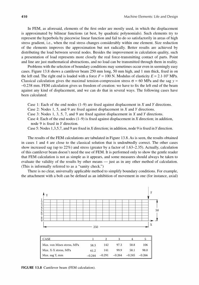
410 Machine Elements: Life and Design
In FEM, as aforesaid, elements of the first order are mostly used, in which the displacementis approximated by bilinear functions (at best, by quadratic polynomials). Such elements try torepresent the hyperbola by piecewise linear function and fail to do so satisfactorily in areas of highstress gradient, i.e., when the real stress changes considerably within one element. Size reductionof the elements improves the approximation but not radically. Better results are achieved bydistributing the load between several nodes. Besides the improvement in calculation quality, sucha presentation of load represents more closely the real force-transmitting contact of parts. Pointand line are just mathematical abstractions, and no load can be transmitted through them in reality.
Problems with the selection of boundary conditions may sometimes occur even in seemingly easycases. Figure 13.8 shows a cantilever beam 250 mm long, 50 mm high, and 1 mm thick, fixed in onthe left end. The right end is loaded with a force F = 100 N. Modulus of elasticity E = 2.1·105 MPa.Classical calculation gives the maximal tension-compression stress σ = 60 MPa and the sag y =−0.238 mm. FEM calculation gives us freedom of creation: we have to fix the left end of the beamagainst any kind of displacement, and we can do that in several ways. The following cases havebeen calculated:
Case 1: Each of the end nodes (1–9) are fixed against displacement in X and Y directions.Case 2: Nodes 1, 5, and 9 are fixed against displacement in X and Y directions.Case 3: Nodes 1, 3, 5, 7, and 9 are fixed against displacement in X and Y directions.Case 4: Each of the end nodes (1–9) is fixed against displacement in X direction; in addition,
node 9 is fixed in Y direction.Case 5: Nodes 1,3,5,7, and 9 are fixed in X direction; in addition, node 9 is fixed in Y direction.
The results of the FEM calculations are tabulated in Figure 13.8. As is seen, the results obtainedin cases 1 and 4 are close to the classical solution that is undoubtedly correct. The other casesshow increased sag (up to 22%) and stress (greater by a factor of 1.63–2.35). Actually, calculationof this cantilever beam doesn’t need the use of FEM. It is performed only to show the gentle readerthat FEM calculation is not as simple as it appears, and some measures should always be taken toevaluate the validity of the results by other means — just as in any other method of calculation.(This is informally referred to as a “sanity check.”)
There is no clear, universally applicable method to simplify boundary conditions. For example,the attachment with a bolt can be defined as an inhibition of movement in one (for instance, axial)
FIGURE 13.8 Cantilever beam (FEM calculation).
F
123456789
CASE
Max. von Mises stress, MPa
Max. X-X stress, MPa
Max. sag Y, mm
1 2 3 4 5
58.3
61.2
–0.244 –0.291
142
141
–0.264
97.3
99.9
–0.245
58.8
58.1
–0.266
106
98.0
Y
X250
50
9563_C013.fm Page 410 Wednesday, July 25, 2007 4:41 PM

Calculations for Strength 411
direction, or a complete inhibition of movement. This inhibition can be replaced by a springyelement that allows movement but provides resistance that is directly proportional to the displace-ment. A constant resistance to displacement can be imposed by application of friction forces. Thesemovement limitations can be supplemented with an inhibition of turn of the connected parts at thispoint, and so on.
The complete inhibition of linear or angular displacement at the fixing points means that theadjoined parts are absolutely rigid. This assumption greatly simplifies the calculation, because thereis no need to determine the compliance parameters of the fixing elements. In many cases thisassumption is justified, but in each particular case it is worth checking whether it is valid.
It is clear that the introduction of pliable fixations in a statically determined scheme is mean-ingless because it doesn’t change anything. In a statically indeterminate system, the calculationwith rigid and pliable fasteners may give surprisingly different results. The influence of theseboundary conditions on the stress pattern of the parts can be investigated by comparing FEMcalculations with different boundary conditions.
EXAMPLE 13.2
A short beam is attached to a base at two points and is loaded by a force F = 10,000 N in themiddle of its length, (see Figure 13.9). The section modulus W of this beam is given by
The bending moment M
FIGURE 13.9 Two-support beam (FEM calculation).
Wb h
mm= = ⋅ =2 2
3
610 50
64167
MF L
N mm= = ⋅ = ⋅ ⋅4
10000 1004
2 5 105.
CASE 3 4 5 6
46.0 59.4 46.0 59.4
kh
kv
khkv
F
31.3
2
25.2
1
200
10
Max. tensile
stress, MPa
50
9563_C013.fm Page 411 Wednesday, July 25, 2007 4:41 PM

412 Machine Elements: Life and Design
Thus, the maximal tension stress, according to classical beam theory (with the usual rollerunder one of the supports), is
This beam has also been calculated using FEM. The attachments have been assumed to bespringy with different rates:
Case 1: kh = kv = ∞Case 2: kh = kv = 100,000 N/mmCase 3: kh = kv = 10,000 N/mmCase 4: kh = kv = 1,000 N/mmCase 5: kh = 10,000 N/mm and kv = 1,000 N/mmCase 6: kh = 1,000 N/mm and kv = 10,000 N/mm
The results are tabulated in Figure 13.9. Comparing cases 3 with 5 and 4 with 6, we see thatonly the compliance in the horizontal direction plays a role in this case. This calculation showsthat the concrete estimation of compliance of the attachments, even if it is rough, may be important.
13.3.4 IS THE COMPUTER PROGRAM CORRECT?
The computer programs are continually improving, and as long as the program is new, it may havesome defects (“bugs”) that have not been revealed. These defects may show up in very specialcases. The usual user is much more likely to make his own errors because of misunderstanding ofsubtleties of the new program. Therefore, it is a usual practice to test the program by solving simplerproblems that have been solved theoretically (known as a closed-form solution), and the formulasare available, so that the correctness of the result can be easily checked.
13.3.5 MORE ABOUT SIMPLIFIED ANALYTICAL MODELS
The simpler the calculation, the less the opportunities we have to make an error. Therefore, one ofthe ways to check the calculation is to make and calculate a simplified analytical model, even ifyour computer is able to calculate the model with no simplifications. The comparison of the resultsis useful. If the results are comparable, this adds to your confidence in your calculations. But ifthe results are dissimilar, there may be three options to think about:
1. One of the calculations (or both of them) may be erroneous; they should be checked forpossible errors.
2. The simplifications may be incorrect or inappropriate to a certain case.3. The computer program has bugs.
The simplifications are often unavoidable, because some problems (for instance, contact prob-lems) may be too difficult to solve using the available computer program. Therefore, the computingengineer is forced to substitute, for example, a rigid fixing point for a real bolt joint. The possibleinfluence of such forced simplifications on the stress condition of the parts should be considered.
Making simplifications, we also can transform the real, complicated problem into a simplerone that has an exact analytical solution (again, a closed-form solution), which can be calculatedmanually to obtain an approximate result. In Chapter 4, Example 4.5 the slope angle of the shaftwas calculated approximately and using FEM, the difference was found to be as great as 19%.
σ = = ⋅ =MW
MPa2 5 10
416760
5.
9563_C013.fm Page 412 Wednesday, July 25, 2007 4:41 PM

Calculations for Strength 413
Example 5.3 and Figure 5.9 (Chapter 5) demonstrate the strength calculation of an end plate.It was made twice: first under the simplifying assumption that the bolt force is distributed evenlyover the bolt centers circle, and then using FEM. The difference in the maximal stress magnitudewas of 25%.
In Chapter 7, Example 7.8 (in the end), the simplified calculation of oil heating has been usedto check the result obtained from an exact formula: the results were identical. Here is one moreexample of the development and use of a simplified analytical model.
EXAMPLE 13.3
A ribbed round plate (Figure 13.10) is supported over its contour and loaded in the center with aforce P = 10,000 N. According to the FEM calculation, the maximal tension stress (on the ribs)equals 140 MPa, and the maximal sag (in the center of the plate) equals 0.182 mm. Are theseresults correct?
Let’s try to calculate this plate using the available formulas for round plates without ribs.3 Tomake such a calculation, we have to replace the ribbed plate by an “equivalent” plate of constantthickness. One sixth of the cylindrical section of the real plate looks as shown in Figure 13.11a.The less the radius of this section, the less is the length L between points A and B and the stifferthe section per unit of length. Let’s calculate the parameters of the equivalent section at the meandiameter d1 = 150 mm. Now, we are going to determine the moment of inertia I and the sectionmodulus W of the real section (about the X–X axis) using one sixth of it presented in Figure 13.11a.The length of arc A–B is
FIGURE 13.10 Ribbed plate.
Ld
mm= = ⋅ =π π1
61506
78 5.
A
B
F
∅150
∅300
5
30
5
9563_C013.fm Page 413 Wednesday, July 25, 2007 4:41 PM

414 Machine Elements: Life and Design
As is known, the neutral line of a section passes through its center of gravity (CG). Thecoordinate Y of the CG is obtained from the equilibrium equation:
whereA1 = 78.5·5 = 392.5 mm2 = area of element 1A2 = 30·5 = 150 mm2 = area of element 2Y1 = Y − 2.5 mm = distance of the CG of element 1 from the X–X lineY2 = 20 − Y mm = distance of the CG of element 2 from the X–X line
From here, Y = 7.34 mm. And now the moment of inertia of this cross section can be obtainedfrom the following formula:
where
FIGURE 13.11 Real section (a) and equivalent section (b) of a ribbed plate.
2
1
Y1
Y2 X X
(a)
(b)
Ymax
L = 78.5
Y
30
5
5
t
A Y A Y1 1 2 2=
I I I A Y A Y= + + +1 2 1 12
2 22
I mm I mm
I
1
34
2
34
78 5 512
8185 30
1211250
81
= ⋅ = = ⋅ =
=
.;
88 11250 392 7 34 2 5 150 20 7 34 452922 2+ + − + − =( . . ) ( . ) mmm4
9563_C013.fm Page 414 Wednesday, July 25, 2007 4:41 PM

Calculations for Strength 415
The section modulus is given by
The equivalent thickness of the plate t shown in Figure 13.11b should be calculated twice: withrespect to rigidity (tr) and to strength (ts). In the first case, the real section and the equivalent oneshould have the same moment of inertia I. For one sixth of the cylindrical section, it is
and from here thickness tr of the equivalent plate is
The maximal sag of the equivalent plate is
whereP = 10,000 N = force applied to the plateν = 0.3 = Poisson’s ratioa = 150 mm = radius of the plate
(Here, E = 2.06 · 105 MPa = modulus of elasticity of the material.)The maximal sag in the center of the plate is
This result amounts to one half of what has been obtained using FEM (0.182 mm).For the stress calculation, the real section of the plate and the equivalent one should have the
same section modulus W. For one sixth of the cylindrical section, it is given by
From here,
WI
Ymm= = =
max .4529227 66
1637 3
78 512
452923
4. ⋅ =t
mmr
t mmr = ⋅ =45929 1278 5
19 13
..
w Pa
Dmax
( )( )
= ++
316 1
2νπ ν
DE t=
−= ⋅ ⋅
−=
3
2
5 3
212 12 06 10 19 1
12 1 0 31 31
( ). .
( . ).
ν⋅⋅ ⋅108 N mm
wmax
( . )( . ) .
.= ++ ⋅
=100003 0 3 150
16 1 0 3 1 31 100 0
2
8π887 mm
78 56
16372
3. ⋅ =t
mms
t mms = ⋅ =1637 678 5
11 2.
.
9563_C013.fm Page 415 Wednesday, July 25, 2007 4:41 PM

416 Machine Elements: Life and Design
The maximal tension stress in the center of the equivalent plate is
This stress is greater by about 30% than that determined using FEM (140 MPa). So in thiscase the simplified model was a rough approximation. Nevertheless, it provides us with the orderof stress and strain magnitudes and thus gives us the desired check of the FEM calculation.
13.3.6 CONSIDERATION OF DEFORMATIONS
The computerized calculation for strength offers the unique ability to visualize the deformationpattern. Each designer imagines these deformations, and, looking at the computer simulation, canfind some discrepancies between the imagined and observed pictures. By this means, gross mistakescan be easily found. For example, if you see some displacement in a point that simulates a bearingor a rigid connection and has been defined as an immovable attachment point, that means therewas a mistake in the boundary conditions data.
The computer picture is not always incorrect; the designer’s imagination can be false, too. Thiscase is nevertheless interesting because it improves our intuition, and supports the notion that visualizingthe deformation pattern is not only a useful tool for fault tracing but also an enthralling occupation.
The deformation pattern is associated closely with the boundary conditions. The latter aresimplified as compared with reality, and this simplification may be irrelevant. Observation of thedeformations may provide the designer with “food for thought” on the validity of these simplifications.
It was shown previously that the boundary conditions may influence considerably the resultsof the stress and strain calculation. The acceptable choice of boundary conditions can be maderelying on the FEM analysis of different options. In some cases, the design of the connection shouldbe changed so as to decrease the influence of boundary condition uncertainties on the stressed stateof the part. Generally, to make the configuration more easy and certain for strength calculationincreases its reliability.
13.4 HUMAN ERROR
You have done a calculation. No matter what kind of calculation it is, the result is the same: yousee formulas and figures, and you don’t know whether it is correct or false. If you have anexperienced supervisor, you go to him. You give him your opus and say as confidently as you can,“Here you are! That’ll do?” But the supervisor looks frostily; to check your work, he has to do ithimself anew, but he has his own work to do. He asks you, “Did you check your calculation?” Agood question, isn’t it? If you had asked for advice, we would have advised you to check yourcalculation thoroughly before being asked this question. But how to do that? When the calculationis complicated (especially when it is hidden inside a computer that makes 1 million operations persecond), the computing engineer often feels himself unable to evaluate its correctness. And thenhe says, “The calculation shows that …” and other words. The problem is that, whatever thecalculation shows, you, and only you, are the one who is responsible for the results of the calculationyou had been charged with. Conclusion: you must somehow check your calculations.
The error you are looking for may appear in any place. It can be just an arithmetic error, falsedimensioning, incorrect definition of boundary conditions, and so on. All this should not drive youto despair; you are able to find any possible errors and to feel completely confident about thecorrectness of your calculations.
13.4.1 ARITHMETIC
Arithmetic errors are among the most frequently occurring. One of the simplest ways to find themis to make the calculation twice or thrice. If each time you have different results, you have to take
σ νmax ( ) . ln .= + +
=Pt
ats s
21 0 485 0 52
1000011..
( . ) . ln.
.2
1 0 3 0 48515011 2
0 52 1842
+ +
= MPa
9563_C013.fm Page 416 Wednesday, July 25, 2007 4:41 PM

Calculations for Strength 417
a rest and repeat the calculation in a day or two. Another way is to simplify the calculation to avoidoutrageous mistakes. For example,
Is this correct? We can write the same figures approximately, and in a simplified form, so as toenable mental calculation:
The next day, you can make the two steps of calculation again to be completely confident ofits correctness.
13.4.2 UNITS (DIMENSIONS)
Before you start making arithmetic errors, you have to decide about the units (dimensions) youuse for the equation members. You should never write any figure without its dimension! For example,you must not write “the speed is 10,” or “the time needed for this operation is less than 3,” or “theforce equals 5000.” Possibly, you remember that the speed is measured in meters per second (m/sec),time in hours (h), and force in Newtons (N), but it should be written each time you write the figure.In this way, you keep feeling the physical essence of the problem and don’t let your mind strayfrom it. For example, if you obtain that the speed equals 5000, it may not attract your attention.But if you see 5000 m/sec, you suddenly remember that it is quite close to the orbital velocity, andit looks a bit unreal for the railway train you are working on.
And this is not enough. When you use a formula, the result depends on the dimensions of theformula members. Therefore, each time you substitute the figures into formulas, it is worth writingseparately their dimensions and checking the dimension of the result. Let’s take, for example,Equation 7.4 and put the torque T1 in N·mm, W in mm, and d1 in mm, the gear ratio i being anondimensional quantity:
If the torque was taken, say, in N·m or lb·in, you can immediately see that the resultantdimension looks unfamiliar, and you will change the dimensions (and, respectively, the figures) toobtain a more reasonable result.
A good way to check the dimensions and the arithmetic at once is to repeat the calculation indifferent units.
EXAMPLE 13.4
Spur gear d1 = 100 mm, d2 = 200 mm, W = 50 mm transmits load of P = 150 kW at n1 = 1500 r/min.Gear ratio i = 2. Torque applied to the pinion is
π ⋅ ⋅ ⋅⋅ ⋅
=203750 18 82 0 00930 294 15800 25 4
0 95, .
. ..
3 2 10 2 10 103 10 2 10 2 10
15 2
1 4
⋅ ⋅ ⋅ ⋅ ⋅⋅ ⋅ ⋅ ⋅ ⋅
≈−
−
KT iW d i
N mmmm mm
Nmm
MPaH = ± = ⋅⋅
= =2 11
12 2 2
( )
TP kWn rpm
N m N m11
9555 95551501500
955 5= = ⋅ = ⋅( )( )
. == ⋅ ⋅
= ⋅ ⋅ +⋅ ⋅
=
9 56 10
2 9 56 10 2 150 100 2
5
5
5
2
.
. ( )
N mm
KH ..74 MPa
9563_C013.fm Page 417 Wednesday, July 25, 2007 4:41 PM

418 Machine Elements: Life and Design
Now, let’s go to another system of dimensions: horsepower (hp), pounds (lb), and inches (in.).
Such a method provides a good way of control, and it also gives us practice in dealing withdifferent dimensions.
13.4.3 IS THIS FORMULA CORRECT?
The calculation can be erroneous not only because of your own errors, but also because the formulasin the books may have misprints. Every time you use a formula, you should be suspicious of andcheck it. You can try and develop it by yourself, or find it in other books (if there are such), butthe first thing is to check the dimensions. For example, if you see the formula
you can immediately notice that in the first term of the equation the power of the stresses is 1 (say,MPa), and in the second term the stress is squared (MPa2). In a perfect formula, terms with differentdimensions can’t be added or subtracted, so this equation is surely false.
When the formula is empirical, the check on dimensions may be useless. For example,Equation 6.8 for elastic deformation of ball bearings
has no physically reasonable dimensions. To obtain the true result, we must know exactly thedimensions of all the equation terms; in this very case, diameter d must be in mm and force Fr in N,then deformation δ1 is obtained in µm.
Empirical formulas can’t be checked by developing; even comparison with other books can beuseless because the false formula can be reprinted in several books with the same error. In suchcases, it is important to find somebody who is experienced in using this formula or to consult theauthor of this formula. If not, some experiments should be made to check the validity of the formula.If you have checked the formula and used it successfully, you can keep this formula (and also thecalculation as an example) for your following professional life.
Sometimes an empirical formula can be checked by analysis of a simplified analytical model.For example, the elastic deformation in the rolling contacts of straight roller bearing NU310E under
P kW HP HP
W in d
= = ⋅ =
= =
150 150 1 36 204
5025 4
1 968 1
.
.. ; == =
= ⋅ =
10025 4
3 937
6 22 10 614
1
..
.( )( )
.
in
TP Hp
n rpm222 10
2041500
8460
2 8460 31 968 3
4⋅ = ⋅
= ⋅ ⋅⋅
lb in
KH . .9937 2832
1 7 02 10
2 2
4
⋅⋅
⋅=
= ⋅ −
lb in
in inpsi
psi kg m. / mm N mm
K MPaH
2 3 2
3
6 89 10
832 6 89 10 5 73
= ⋅
= ⋅ ⋅ =
−
−
. /
. .
F e( ) [( ) ( ) ( )]σ σ σ σ σ σ σ σ= − + − + − −16
131 2 2 3 1 3
2
δ µ12 30 153 0 00044= −( . . ) /d F mr
9563_C013.fm Page 418 Wednesday, July 25, 2007 4:41 PM

Calculations for Strength 419
radial load Fr = 10,000 N, when calculated using the empirical formula in Equation 6.9 (Chapter 6),is given by
In Chapter 6, Example 6.2 (Subsection 6.2.2) is shown how this deformation can be calculated.The summary deformation in rolling contacts
Thus, this empirical formula is okay.You may ask, ‘‘Okay, but what shall I take for my consequent calculations: 13 µm or 17 µm?”
The point is that both the empirical formula and the checking calculation are approximate, and itis worth taking the worst result. Virtually, the difference of 4 µm is not significant in generalapplications. When it is important, indeed, both the empirical formulas and approximate calculationsmay be unacceptable, and experimental research of the deformation should be undertaken.
REFERENCES
1. Harris, C.M., Shock and Vibration Handbook, 2nd ed., Harris, C.M. and Crede, C.E., Eds., McGraw-Hill,New York, 1976.
2. Juvinal, R.C., Engineering Considerations of Stress, Strain and Strength, McGraw-Hill, New York,1967.
3. Timoshenko, S. and Woinowsky-Krieger, S., Theory of Plates and Shells, McGraw-Hill, New York,1959.
δ µ1
0 065 0 06550
10000 13= = =. .d
F mr
∆ ∆C i C o mm m, , . . .+ = + = =0 0085 0 0085 0 017 17 µ
9563_C013.fm Page 419 Wednesday, July 25, 2007 4:41 PM

9563_C013.fm Page 420 Wednesday, July 25, 2007 4:41 PM

421
14
Finale
Pussy cat, pussy cat, where have you been?I’ve been in London to look at the queen.Pussy cat, pussy cat, what did you there?
I frightened a little mouse under her chair!
Our book is finished, and it is a pity, as we have been able to show you only as much as a littlemouse from the “Great Kingdom of Machinery.” We sought to tell you some basic facts abouttypical machine elements: their life, design considerations, and fundamentals of calculations.Evidently, we were unable to do more (in the context of the declared subject matter) because ourtime resources, knowledge, and experience are limited. But, the abilities and experience of thefellowship of mechanical engineers are immensely greater, and each of us has had the happy chanceof putting a brick in the Great Chinese Wall of collective knowledge.
Our goal was to give our readers (especially those whose experience is limited) some ideas toform the basis for their own research effort. We would highly appreciate any feedback on this bookfrom you: remarks, interesting cases, and examples backing or contradicting what is written in thisbook. To learn from your experience would be a great reward for our work.
“The worst beginning is better than the best end,” said Shalom Aleichem. This book has beenfinished, with our regrets. But your creative accomplishments and ours as well begin every morning,and the end is far away. Let’s go forward!
9563_C014.fm Page 421 Wednesday, July 25, 2007 4:42 PM

9563_C014.fm Page 422 Wednesday, July 25, 2007 4:42 PM

423
Index
A
Abrasive wear, 115, 171, 192Action, line of, 161, 163–164, 195Addendum.
See
ToothAdmissible stress, 86, 356–359, 364, 387, 389, 391–392,
394–395, 404Alignment, 8, 56, 58, 104–105, 197, 236, 249, 253–255,
265, 274angular, 85, 96, 106, 109–110, 121, 331, 344–345radial, 330of shaft, 119, 329–334techniques, unit connections, 333of teeth, 197
Aluminum alloy, 19, 46, 110, 143, 151, 245, 297, 316, 323, 325, 380
Anglehelix, 76, 103–104, 165–166, 193, 197–198, 219, 224,
236pressure, 96, 103, 117, 160, 168, 173, 186, 196, 220slope, 60, 63, 65, 357, 384, 412
Angular misalignment, 345effect on shaft, bearing loads, 331
Arrangement, of bearings, 121–123, 130Assembled gears, 238Attachment point, 278, 280, 282, 291, 416Axial fixation, shafts, 104Axial force (load), 5, 8, 13–14, 63, 67, 71, 74–75, 80–84,
103, 115–123, 129, 132–133, 136–137, 141, 152, 197–198, 219–220, 227, 236, 246, 249, 255, 274, 301, 311, 339, 342, 408–409
Axles, 3, 44, 71, 106, 137, 200, 241, 273, 284, 357
B
Babbit alloys, 143–144, 149, 151Backlash, 102–103, 198–199, 242
gear mesh, 198–200Ball bearing, 108–109, 117–118, 129, 132, 134–135, 255,
374, 418Bandage gears, local slippage, 229Base circle, 160–161, 163, 195Base pitch, 160–161, 163, 169, 181–182, 195–196Basquin’s formula, 382Beam supports, strength calculations, 408Bearing stress, 86, 92–93, 95–96, 100–101, 296Bearing surface, 84, 141, 146, 149, 151, 293, 295–298,
300–301, 311, 318Bearings
adsorbed oil film, 138alignment, 119, 151–152, 249arrangement, 122–123
axial movement under load, shaft misalignment from, 119
ball, 51, 108–109, 117–118, 123, 129, 132, 134–136, 255, 374, 418
clearance in, 117comparison of, 111cylindrical roller, axial load, 116diesel engine crank mechanism, oil ducts, 157double-row, 56elastic deformation, 133–135failure, 108, 111–115fits, 44, 123–131flat working surface, sliding thrust, 150four-point ball, 123, 136Hersey-Stribeck diagram, 140high-speed roller, compared, 111hollow shaft, 152, 154housing oil ducts, 154hydrodynamic oil film, sliding, 141load distribution, 57, 128lubricated surfaces, contact of, 139lubrication of, 137–140needle, 110oil distribution grooves, 146–147oil supply, plain, spline connections, 157planet wheel, sliding, 148radial, 117radial ball, assembling, 109ring fastening, 129roller without inner rings, 135rollers, ring, shaft, interaction, 124rolling, 108–138rotating oil pressure, 155self-aligning, 151–152self-made roller, 136shaft shoulder height, 133sliding, 138–158, 197straight roller, 106, 110, 113, 116–118, 120–121,
134–136, 418tapered roller, 118–119, 122, 129–130, 132, 134, 255,
270two-cylinder contact, stresses in, 112two-row, 110types of, 108, 140–141
Bending deformation, 4, 7, 25, 56, 58, 67, 152, 181, 217–219, 227, 247, 250, 273, 282, 310, 318, 329, 365
gears, failure, toothed rim, 218straight beam, 25
Bending momentbetween bearings, angular deformation, 59bolts, 291
9563_C015.fm Page 423 Monday, July 30, 2007 6:58 PM

424
Machine Elements: Life and Design
Bending strength, 4, 44, 161, 169–170, 173, 176, 179, 181, 183–187, 192, 199, 232, 240, 348
Bending strength of teeth, 232Bending stress, 14, 37–39, 56, 75–77, 84, 91, 166,
168–169, 181–183, 185–187, 193–194, 197, 218, 249–250, 267–268, 310–311, 331, 357, 359, 364, 390, 399
Bevel gears, 107, 136, 179–180, 186, 200, 208, 238–239, 252–253, 256
Block brake, 5Bolted connections, 11, 14–19, 226, 256, 277–319, 368,
403–404aluminum parts, 296bending, threads, 318bending moment, 291bolt design comparison, 298bolt joint loaded in tension, bending, analytical model,
288bolt shank, maximal, average tension stresses, 304bolt tension force, eccentric, coaxially applied loads, 303bolted joints loaded in shear, load distribution in,
282–287center of gravity, 285center of rotation, 285comparative calculations of, 292cone-fitted bolts, flange connection with, 293contours, complex, 290fastener strength, 313–319
fatigue strength, 317–319static strength, 313–317
fitted bolts, connection with, 307flange connection
slip in, 310types, 306
helical insert for thread reinforcement, 316high fatigue strength bolt design, 318load distribution, loaded in tension, 287–292load distribution between bolts, 278–292loaded in shear, 283loaded with shear forces, 305locking fasteners, 300long stud bolt vibrations, 312parallelogram of forces, false use, 281rib, 279statically determinate, indeterminate beams, 280thin-walled tubes, flange connection of, 278tightened bolt connection, stress distribution, 297tightening of bolts, 292–302
accuracy, 292–295stability of tightening, 295–299
working load, tightening force of bolt, correlation, 302–313
bending load, 311–313load normal to joint surface, 302–305shear load, 305–311
Bolted jointconcentric, eccentric loading, 16concentrically loaded, 16eccentrically loaded, 16two part, 14
Boltscentrically loaded, 16–18, 282eccentrically loaded, 16, 18–19, 303elongation, 294fitted, 226, 282, 287, 307–309, 316, 319locking of, 300–302stability of tightening, 295–302strength
fatigue, 317–319static, 313–317
tapered, 309–310tightening, 292–302
accuracy, 292–295tightening accuracy, 292–295tightening force, 257, 278, 302–313tightening torque, 80–81, 83–84, 292–295, 301, 306, 313working load, tightening force of bolt, correlation,
302–313bending load, 311–313load normal to joint surface, 302–305shear load, 305–311
Boundary condition, 85, 241, 292, 409–411, 416Brake, 4–5, 130, 292Broaching, 71Broken sections, 26Bronze, 95, 107, 143–144, 146, 148, 316Buckling, 46Built-up gear wheels, 224–235Burnishing, 20, 37–38, 53
C
Cage, 107–111, 115, 123, 136–137Cantilever beam, strength calculations, 407
finite element method, 410Carburizing, 20, 44, 101, 132, 239, 265, 270Case hardening, 115, 184, 225Cast housing, 153, 173, 245–246Casting materials
cast steel, 244–245gray cast iron, 31, 200, 221, 232–233, 244–245, 260,
293, 316Centrifugal force, 8, 74, 102, 110, 115, 137, 155–156, 201,
275Change of clearance, unit connections, driving/driven teeth,
349Chrome plating, 270Clearance, 3–5, 8, 18, 56–57, 70–71, 78, 85, 95, 98,
103–105, 107, 115, 117–120, 122–123, 126–129, 131, 133–135, 141, 145, 149, 151–152, 198, 235–236, 263–265, 267–269, 272–273, 294, 305, 309, 318, 329, 332–333, 343, 348–349
Coating, 20, 137, 141, 143, 173, 243–244, 271, 295Coefficient, 18–19, 27–28, 31, 64, 67–69, 72, 74–77,
79–81, 83, 89, 95, 117, 120–121, 125, 127, 134–135, 139–140, 143–144, 171, 183, 228–230, 232–234, 264, 272, 278, 293–295, 301, 305–308, 315, 317, 357, 379–380, 382–384, 386, 393, 404
of friction, 69, 72, 74–77, 79–80, 83, 95, 120, 139–140, 228–229, 232–233, 293, 295, 306–307, 315, 350
9563_C015.fm Page 424 Monday, July 30, 2007 6:58 PM

Index
425
Cold rolling, residual stress distribution after, 37Cold working, 44, 53Combined load, 117, 119Comparative calculations, 175, 187, 226, 231, 282, 284,
292, 390Compliance, 7, 15, 17–18, 44, 57, 72, 97, 125, 131,
151–152, 187, 217–218, 279, 282–283, 291, 298–299, 302–303, 313, 330, 336, 404,411–412
Compressive force, 18, 226Compressive stress, 15, 20, 35–39, 50, 53, 112, 172,
184–185, 227Computer program, 58, 149, 241, 355, 397, 403, 407,
412Conical gears, rigidity with, 222Connections
alignment techniques, 333bolted, 11, 14–15, 19, 226, 256, 277, 279, 281, 283,
285, 287, 289, 291–295, 297, 299, 301, 303,305, 307–309, 311, 313, 315, 317, 319, 368, 403–404
change of clearance, 349crowded tooth, contact patch, 352crowned teeth shape, 345deformations, 322, 324design, 322enlarged tooth length, 348flange, 103–104, 275, 277–278, 292, 303, 305–306,
308–310, 319, 342frame twisting, 323gear coupling, 343hobbing, 346housing connections, 321–329interference fit, 102shaft connections, 329–352splined, 93stress calculation, 324tapered, 67–68, 73, 80
Contact length, 113Contact line, 113, 165–169, 174, 177, 188, 194Contact patch, unit connections, crowded tooth,
352Contact pattern, 107, 253–254Contact pressure, 13, 20, 51–53, 69, 96, 230, 303Contact ratio, 161, 163, 165–166, 194–196Contact seals, 264–274
lip-type seals, 269–271mechanical seals, 272–274O-rings, 268–269piston ring packing, 265–268
Contact strength, of teeth, 174–181Contact stress, 100, 110, 112, 117, 129, 168–169,
173–174, 176, 179, 183, 193loaded tooth, 168
Cooling, 74, 103, 131, 149, 173, 200, 206, 208–212,247, 270–271, 273–274, 338, 343
gears, 208–212Copper alloys, 146, 209, 266, 293Copper platingCotter pin, 206, 300
Couplings, 20, 43–44, 68–69, 95, 104, 156, 174, 197, 208, 292–293, 321–323, 331, 334, 336–343, 347–352, 398
gear typeresilient, 292, 336, 342rigid, 68, 334
Crack propagation, 387Critical frequency, 45, 312–313, 336, 399, 403Critical load, 18Crowned teeth, 343, 345–346, 352Crystal cell, 22Crystal lattice, 21–24, 172, 357, 376, 380
imperfections, 22Crystal structure, 21Crystals, in metal structure, 23Cyclic load, 24, 31, 36, 91, 111, 148, 277, 311, 398Cyclic properties, 391Cylindrical roller bearing, axial load, 116
D
D’Alembert principle, 166Damage accumulation, 404Damage to joint surfaces, rigid connections, movements in,
11–20bolted connections, 14–19bolted joint
concentric, eccentric loading, 16two part, 14
eccentrically loaded bolted connection, deformations, 19fretting, strength-damaging effect, 20interference-fit connection, self-dismantling under
bending load, 14interference-fit connections, 11–14
load distribution nonuniformity, 13loaded with bending moment, 12–14loaded with torque, 11–12torsional deformation, 12
mating surfaces, slip area, damage to, 19–20tightened bolt connection, forces in, 16
Dead center, 3Dedendum.
See
ToothDeflection, 17, 54, 58, 84, 151, 196, 325, 332Deformation
bending, 4, 7, 25, 37, 39, 56, 58–60, 67, 152, 181, 217–219, 227, 247, 250, 273, 282, 310, 318, 329, 365
elastic, 4, 8–9, 19, 24–35, 65, 68, 93, 104, 110, 112–114, 117–118, 122, 131, 133–135, 142, 151, 168, 187, 196, 215, 219, 229, 241–242, 263, 273, 297, 299, 307, 315, 333, 349, 418
elasto-plastic, 32–36housings, 254–255mated part surfaces, 3–9shafts, analysis, 58–65stress patterns, machine components, 21–39
bending deformation, straight beam, 25bending stresses, T-beam, 37broken sections, 26burnishing shafts, roller shapes, 38
9563_C015.fm Page 425 Monday, July 30, 2007 6:58 PM

426
Machine Elements: Life and Design
cold rolling, residual stress distribution after, 37crystal cell, 22crystal lattice, 22crystals, in metal structure, 23dislocation, movement under load, 22elasto-plastic deformation, parts, 32–36elasto-plastic deformation effectiveness, 34filleted bar, strain distribution, 28grains in metal structure, 23metal strength, 21–24metal structure, 21–24notched strip in tension, stress concentration, 30plane sections, 26reversed bending, loss of residual stress from, 39shot peening, residual stress distribution after, 37straight bar, strain distribution, 26stress-strain diagrams, 32surface plastic deformation, 36–39thin-walled beams, deformation of, 25
surface, plastic, 36–39, 53, 190, 295unit connections, 322, 324
Deformation pattern, 29, 278, 281, 287, 416Design
elements, shafts, 46–53of housings, 248–254unit connections, 322
Diagram, stress-strain, 32, 360Diameter, pitch, 63, 100, 160, 167, 179, 183, 186, 220,
232–233, 350Diametral pitch, 96, 136, 160, 181, 183Dimension factor, 90Disk thickness, gears, 221Disk-type gears, deformation, 219Dislocation, 21–24, 31, 380
movement under load, 22Displacement, 1, 4, 8, 23, 56, 85, 93, 98, 101–102,
104–105, 115, 122, 132, 145–146, 152, 154, 158, 173, 183, 194, 198–199, 229–230, 236, 238–239, 251, 255–256, 263, 307–308, 319, 332, 401–402, 405, 407–411, 416
Distortion, 110–112, 115, 132, 143, 172, 238Distribution, load, 1, 3–9, 11–13, 56–58, 65, 76, 85–195,
197–198, 200, 213, 217–220, 223, 226, 241, 250, 255, 257, 277–292, 301, 317–318, 336, 338–340, 349–350, 352, 403
Double-helical gears, 103, 197–199, 235–236bearings or, 197load distribution, 197–198overload factor, 198
Double-reduction gear, shaft-to-hub connections, intermediate shaft, 76
Double-row bearings, 56Durability, 20, 31, 51, 69, 108, 176, 270, 355–356, 359,
374, 384–385Dynamic analysis, 195, 397Dynamic factor, 76, 182Dynamic load, 76, 131, 175, 182, 185, 195–196, 398
E
Eccentric loading, 19, 303Eccentricity, 104, 107, 263
Efficiency, 159, 204, 208, 210–212Elastic deformation, 4, 8–9, 19, 24, 32, 34–35, 65, 68, 93,
104, 110, 112–114, 117–118, 122, 131, 133, 142, 151, 168, 187, 196, 215, 219, 229, 241–242, 263, 273, 297, 299, 307, 315, 333, 349, 418
shafts, gear rim displacements, 8Elastic elongation, 32, 299Elastic range
deformation beam, 33deformations in, 24–31
Elasto-plastic deformation, 32–36effectiveness, 34parts, 32–36
Elasto-plastic rangedeformation beam, 33torsional deformation, 35
Elastomeric spider, flexible coupling, 337Elements of machines, 41–353Elliptic fillet, 318Elongation, 6, 17, 26, 28, 30, 32, 268, 294, 296, 299, 315,
361, 378, 386, 396, 406elastic, 32, 299plastic, 32, 315
Endurance limit, 365Energy loss, 24, 210, 264, 270Engineering stress, 377–378Enlarged tooth length, unit connections, 348Equivalent number of cycles, 178, 375–376Equivalent radius, 113, 168–169, 174Equivalent stress, 83, 91, 306, 314–315, 327, 362, 371–373,
385Escalator drive unit, foundation for proof test, 328Escalator main drive, 62–63External loads, strength calculations, 397
F
Face, gear, load distribution across, 218Face width, 8, 54, 63, 65, 106, 165–166, 168, 171, 174–175,
179–182, 185, 187, 190, 192–195, 198–200, 205, 213, 217, 219–220, 224, 228, 347
Factorof load distribution, 175of safety, 127, 287, 368
Failuresof bearings, 108, 111–115of gears, 170–173, 176, 218
Fan cooling, 208Fasteners, 102, 282, 292, 295–296, 300–301, 311, 313–319,
411fatigue strength, 317–319static strength, 313–317
Fatiguehigh cycle (HCF), 364, 376, 395low cycle (LCF), 363–364, 376, 378, 384–385, 391
Fatigue crack, 6, 11, 19, 37, 71, 86, 114, 170, 172, 215, 218, 292–293, 317, 363–364, 377, 387
Fatigue failure, 51, 177, 218, 358Fatigue life (strain method), 376–386Fatigue limit, 18, 51, 53, 90–91, 112, 143, 177–178, 317,
357, 364–365, 367, 374, 376, 387–390, 396
9563_C015.fm Page 426 Monday, July 30, 2007 6:58 PM

Index
427
Fatigue strength, 13, 19, 37, 44, 51–53, 68, 79, 88–89, 313, 317–318, 357, 359, 361, 363–374, 382, 384, 387, 390, 395–396
Fillet radius, 29, 38, 47–50, 53, 86, 89, 184, 219, 318Filleted bar, strain distribution, 28Finish.
See
Surface finishFinite element method (FEM), 7–9, 15, 30, 54, 73, 85–86,
88, 90, 97, 169, 181, 183, 185, 194, 231, 241, 278, 282, 286–287, 290–291, 299, 303, 305, 321, 403–416
boundary condition interpretation, 409–413computer program, 412deformations, 416design principles, precision, 405–407model design for, 407–409simplified analytical models, 412–416
Fits for rolling bearings, 123–131Flange attachment, gear, 223Flange connection, 103–104, 275, 277–278, 292, 303,
305–306, 308–310, 319, 342Flat working surface, sliding thrust bearing, 150Flexible coupling
with pins, rubber sleeves, 336with rubber pads, 337
Flexible couplings, with elastomeric elements, 341Forced-feed lubrication, 203–206Forces
in tightened bolt connection, 16Four-point ball bearing, 123, 136Fragility, 170Frame strength, 322Frame twisting, unit connections, 323Frequency, natural (critical), 45, 312–313, 336, 399, 403Fretting, 19–20, 51, 53, 65, 68, 71, 88, 95, 127, 144, 215,
217, 278, 292–293, 364strength-damaging effect, 20
Friction coefficient, 19, 67–68, 72, 74–75, 89, 117, 121, 125, 127, 140, 171, 228, 230, 234, 264, 272, 278, 294, 301, 305–306, 308, 315, 339, 351–352
static, 74Friction force, 11, 14, 72, 75, 79, 89, 91, 93, 110, 117, 120,
124–125, 138, 164–167, 171, 173–174, 197–198, 223, 226, 228–229, 268, 270, 272, 277, 282, 285, 287, 292, 294, 301, 305–310, 338, 350, 411
Friction modes, 139–140, 270Function of housings, 241–243
G
Gearsassembled, 238backlash, 198–200
gear mesh, 198–200bandage, local slippage, 229bending deformation, failure, toothed rim, 218bending stress, 187
loaded tooth, 168in tooth root, load distribution influence, 194
bevel, 207, 238–239bevel gears, 238–239built-up gear wheels, 224–235
clearance, 237conical, rigidity with, 222contact stress, loaded tooth, 168cooling, 208–212cooling process, 209coupling
bending moment, 350unit connections, 343
misalignment, 343couplings, 342–352design, 215–240disk thickness, gears, 221disk-type, deformation, 219double-helical, 197–198double-helical ear, 235double-helical gear, overload factor, 198double-helical gears
bearings or, 197load distribution, 197–198
face, load distribution across, 218flange attachment, 223gear, shaft, connection, 216gear mesh, factor, dynamic load, 195–197gear tooth failures, 170geometry, 160, 162, 197geometry of, 160–167grinding wheels types, 237heating process, 209helical, 164–168, 176, 178–180, 186, 198–199, 206,
217–224, 227, 238, 240, 255helical gear, 217–224hobbing machine, double-helical gear, 235involute teeth geometry, 160kinematics of, 160–167leading, lagging surfaces in contact, 165load distribution unevenness across face, 87–195local separation, rim from center, 232lubrication, 200–207lubrication grooves, scraper, 203manufacturing requirements, 235–238mesh, backlash, 198–200non-surface-hardened teeth, fatigue life line, 178number of teeth, tooth shape dependence on, 161oil bath lubrication, gears, 200oil collector, lubrication holes, 203oil level indicators, 204oil spray, direction on gears, 206oil sprayers, 205output shaft, 46pinion shaft design, 216pitch change, from deflection under load, 196pitch deviations, tooth impact by, 195pump, gears, 55ratio, 76, 163, 179–180, 202, 417ribbed wall, stresses in, 228rim, 170, 238
center of gear, connections, 225shaft with, 215–217shapes, 217shrink-fit connection between rim, center, surface
pressure, 230
9563_C015.fm Page 427 Monday, July 30, 2007 6:58 PM

428
Machine Elements: Life and Design
sketch, 7spur, 99, 107, 116, 160–164, 166–169, 171, 174, 176,
181, 186, 195–196, 199, 206, 213, 217–226, 238, 240, 417
spur gear, 217–224spur gear geometry, 162spur gear teeth, helical teeth, contact lines, 167spur gearing forces, 167–169stress amplitude, number of cycles to failure,
dependence, 176teeth, 8, 36, 44, 63, 76, 96, 99, 103, 132, 136, 160–161,
167–169, 172, 174–187, 196, 205, 215, 228, 237, 239–240, 242, 253, 255
bending strength, 181–187contact strength, 174–181stresses in, 167–169
teeth design, 239–240teeth machining tools, clearing space, 237tooth design, 239tooth engagement, 162tooth failure, 170–173tooth failures, 170tooth load, 167tooth misalignment, load distribution, contact line, 188tooth root shape, grinding influence, 184tooth spaces, oil drain, 199types, 216uneven load distribution, gear sensitivity, 190vertical output shaft, two-stage bevel-planetary gear,
207wear-prone gear, run-in process, 191welded, 225welded to shaft/hub, 217
Geometry of gears, 160–167Gerber failure line, 369Goodman diagram, 367–368Grains in metal structure, 23Gravitation, 241, 409Gravity, center of, 251, 282–283, 285, 324, 414Grease lubrication, 101, 137Grinding wheels types, 237Grooves in bearings, 146–147
H
Hardened layer, 20, 50, 53, 114–115, 135–136, 170, 172–173
Hardness, 44, 68, 101, 111, 116, 127, 135, 137, 142–144, 151, 172–173, 176–178, 180, 182, 186–187, 190, 221, 244, 260, 265–266, 301, 309, 337, 339, 359, 361–362, 364, 384, 395–396
steel mechanical properties, 362Harmonic drive, 208Heat transfer factor, 208Heat treatment, 43, 112, 172, 184, 222, 225, 227, 237–238,
240, 242, 246–247, 270, 361, 384, 387, 391, 395–396
Heating, 8, 38, 74, 78–79, 111, 131, 138, 172, 200, 209–211, 262, 271, 338, 413
of gears, 209of rubber elements, 338
Helical gear, 164–166, 168, 176, 178–180, 186, 198–199, 206, 217–224, 227, 238, 240, 255
Herringbone gear, 197–198Hertzian stress, 114, 135, 168, 171, 174–175, 177
loaded tooth, 168Hertz’s formula, 168, 174High-speed roller bearings, compared, 111Hob radial motion, tooth thickness, relationship, 347Hobbing, 235–236, 346Hollow shafts, 46, 51–54, 131–132, 152, 154, 334–335
deformation, 152design, 52oil supply through, 154
Hooke’s law, 377–378, 389, 405–406Housing
connections, 321–329deformations, 254–255design, 8, 248–255function, 241–243material, 243, 245–246materials for, 243–247nonsplit, 253–254seals, 255–275split at right angle to axes of shafts, 251–253split through axes of shafts, 248–251
lifting elements, 251mounting feet, 250–251
stiffness, 254–255Hub strength, 90–91Human error, strength calculations, 416–419
arithmetic, 416–417units, 417–419
Hydrodynamic, 9, 139–141, 149–152, 155–156, 174, 206, 275
oil film, 9, 141Hypotheses, of plane cross section, 24–25, 33Hysteresis loop, 380, 382
I
Idling gears, 161, 336–337Impact load, 108, 170, 181, 243–244, 336Impact toughness, 359, 396Imperfections of crystal lattice, 22Induction hardening, 20, 53, 101, 228Interference fit connections, 102Interference-fit connections, 11–14
friction coefficient, 74–77load distribution, 13load distribution nonuniformity, 13loaded with bending moment, 12–14loaded with torque, 11–12self-dismantling under bending load, 14shaft-to-hub connections, 67–69, 71–79
design, 77–79easily disassembled, 69
slippage, 13torsional deformation, 12
Internal stress, 24, 31, 37, 246–247, 332Involute profile of teeth, 161, 184, 196Involute teeth geometry, 160
9563_C015.fm Page 428 Monday, July 30, 2007 6:58 PM

Index
429
J
Jam nuts, 300Joints
bolted, 11, 14, 16, 20, 226, 240–241, 287, 319, 403keyed, 67loaded in shear, 277, 282–283, 287, 310, 341loaded in tension, 14, 254, 282, 287–288, 359, 405separation of, 245, 254–255, 277splined, 67, 70, 93
Journal, shaft, 56, 69, 104, 107, 141, 143–147, 149, 153, 236
K
Key displacement, shaft-to-hub connections, 85Key joints
design, strength calculation, shaft-to-hub connections, 79–93
hub near keyway, strength, 88–92keys, strength, 85–86role of interference-fit connections, 79–85round keys, 92–93shaft near keyway, strength, 86–88
hub strength, 79–93keys strength, 85–86shaft strength, 86–88shaft-to-hub connections, 69–70
Key-joints, 67Keyed hub, stress in, shaft-to-hub connections, 88–89Keyway deformation under load, shaft-to-hub connections,
88Keyway end, stress concentration, shaft-to-hub
connections, 87Kinematics, 5, 160, 183, 256, 399
L
Labyrinth seal, 206, 269, 274Lame formula, 126Layout of shaft loading scheme, 54–58Leading, lagging surfaces in contact, 165Leading surfaces, 165, 171Leak-proofness, 275Length of action, 161, 173, 183Length of contact, 113Life factor, 176–177Life prediction, 355, 364, 395, 404
machine parts, 421metal part strength, 357–396strength calculations, 397–419
Lifting device, 4Lifting drum, with driving shaft, strength calculations, 398Lifting element, 251Limited fatigue life, irregular loading (stress method),
374–376Linear expansion factor, 78, 245Lip-type seals, 269–271Load
cyclic, 24, 31, 36, 91, 111, 148, 277, 311, 398impact, 108, 170, 181, 243–244, 336
Load capacity, 31, 34–35, 37, 44, 58, 67–70, 74–75, 77, 89, 92, 106–107, 110, 112, 128–129, 140, 147, 149, 151, 163, 166, 170–172, 179, 238, 251, 300–301, 307, 309, 318, 404
Load distributionacross face, 87–195along the teeth, 7–8, 65, 96–97, 99, 106, 170, 190between the bolt, 223, 226, 277–278, 403bolted joints loaded in shear, 282–287between bolts, 278–292double-helical gear, 197–198mated part surfaces, 3–9between the teeth, 96–97, 99–100, 350unevenness across face, gears, 87–195
Load distribution factor, 189, 194Loading layout, shafts, strength analysis, 54–58Loading types, strength calculations, 401Locking fastener, 300–301Long addendum design, 161, 183, 186Loose spline joint lubrication, shaft-to-hub connections,
101Low-cycle fatigue, 363, 376, 378, 384–385, 391Lubrication
bearings, 137–140forced-feed, 203–206gears, 200–207grease, 101, 137grooves, scraper, 203pressure-fed, 107splash, 107, 201spline joint, 101
M
Machine element strength, 386–390dimensions of part, 387–388stress concentration, 388–389surface finish, 387
Machine parts, life prediction, 355–421Magnesium alloy, 221, 245, 296, 301Manufacturing requirements, 235–238Margin of safety, 170, 173Mated part surfaces, deformations, load distribution, 3–9Materials for housings, 243–247Mating surfaces, slip area, damage to, 19–20Maximal principal stress, 88Maximal stress, 24, 27–31, 48, 77, 83, 85, 89–90, 171, 268,
303, 305, 317, 319, 357, 364, 367, 370–371, 374, 376, 389, 398, 404, 413
Mean stress, 31, 90–91, 317, 364, 366–367, 369–371, 373, 385
Mechanical properties, 34, 53, 245, 267, 317, 359, 361–362, 387, 395
Mechanical seals, 272–274Mesh, gear, factor, dynamic load, 195–197Metal strength, 21–24, 357–396
bending loads, bars subjected to, stress distribution, 387comparative calculations, 390–395cyclic stress-strain curve construction, 381fatigue life (strain method), 376–386fatigue limit
vs.
mean stress, Goodman diagram, 367
9563_C015.fm Page 429 Monday, July 30, 2007 6:58 PM

430
Machine Elements: Life and Design
fatigue strength (stress method), 363–374hardness, steel mechanical properties, 362hysteresis loops, cyclic deformation transition period,
380limited fatigue life, irregular loading (stress method),
374–376machine element strength, 386–390
dimensions of part, 387–388stress concentration, 388–389surface finish, 387
maximal stress,
vs.
mean stress, Serensen diagram, 370monotonic, cyclic stress-strain curves, differences, 382real material strength, 395–396rotating-bending endurance test machine, 366shaft with fillet, 393static load, strength at, 259–363strain-life curves, 383stress-strain diagram, 360stress variation with time, 365stresses, frequencies, spectrum, 375tensile test specimen, 360
Metal structure, 21–24Micro-slip, 229Miner’s rule, 374Minimal stress, 366Misaligned hubs, 344Misalignment
angular, 85, 96, 106, 109–110, 121, 331, 344–345of shafts, 329
Modification of profile, 170, 173, 196, 239Modulus
of elasticity, 5, 24, 26, 32, 34, 45, 60, 72, 113, 125, 139, 144, 168–169, 175, 193, 230–231, 242, 244–245, 258, 260, 267, 281, 298, 308–309, 312, 314, 318, 325, 330, 342, 378, 384, 391, 408, 410, 415
of section, 46, 411, 413, 415Moment of inertia, 12, 45, 60, 64, 258, 260–261, 267, 281,
314, 323, 325–326, 330, 408, 413–415Monotonic loading, 379–381Movable joints, sealing, 262–275
combined seals, 274–275contact seals, 264–274
lip-type seals, 269–271mechanical seals, 272–274O-rings, 268–269piston ring packing, 265–268
noncontact seals, 262–264Movements, rigid connections, joint surface damage, 11–20
bolted connections, 14–19bolted joint
concentric, eccentric loading, 16two part, 14
eccentrically loaded bolted connection, deformations, 19fretting, strength-damaging effect, 20interference-fit connection, self-dismantling under
bending load, 14interference-fit connection slippage, 13interference-fit connections, 11–14
load distribution nonuniformity, 13loaded with bending moment, 12–14
loaded with torque, 11–12torsional deformation, 12
mating surfaces, slip area, damage to, 19–20tightened bolt connection, forces in, 16
N
Necking, 359, 361, 378Needle bearing, 110Neuber’s formula, 388Neutral axis, 26, 34, 36, 289Nitriding, 20, 44, 53, 101, 132, 172, 193, 225, 227, 266, 270Non-surface-hardened teeth, fatigue life line, 178Noncontact seals, 262–264Notched strip in tension, stress concentration, 30Number of cycles, 107, 176–179, 190–191, 357–359,
363–364, 374–376, 383–384, 390–395,398–399
Number of reversals, 383Number of teeth, 93, 96–97, 160–161, 165, 183, 186,
194–195, 239tooth shape dependence on, 161
Nuts, 4, 16, 46, 68–69, 79–83, 94–95, 122, 128–129, 206, 215, 248, 264, 293–298, 300–302, 307–308, 310–311, 314–318, 336, 404
O
O-rings, 256, 262, 264, 268–269, 272–274Offset, 8Oil bath lubrication, gears, 200Oil collector, lubrication holes, 203Oil-distributing grooves, 146, 154, 156–157Oil distribution, 146–147Oil level indicators, 204Oil spray, direction on gears, 206Oil sprayers, 205Oil supply, 101, 201, 206, 313
plain bearings, spline connections, 157Oil wedge, 116, 139–140, 146–147, 149–153One-pair engagement, 161Outside diameter, 161, 163, 296Overhung bending moment, angular deformation, 60Overhung force, 59Overhung radial force, angular deformation, 59Overload factor, 198
P
Palmgren-Miner rule, 374Parallel link mechanism, 3, 242Parametric excitation, 165, 195, 222Parametric resonance, 195Pattern
deformation, 21–39, 278, 281, 287, 416strain, 26, 28, 32stress, 21–39, 174, 194, 409, 411
Pin, 9, 51, 54, 91–93, 107, 132, 145–146, 149, 151, 153, 156, 206, 208–211, 226, 238, 245, 249, 272–273, 282, 287, 300, 302, 307–308, 315, 336, 338, 340, 350–351
9563_C015.fm Page 430 Monday, July 30, 2007 6:58 PM

Index
431
Pinion, 7–8, 43, 54, 63, 65, 76, 95, 103–105, 107, 122, 133, 161, 163, 169, 173–176, 178–180, 183–184, 186, 194–195, 197–198, 210, 215–216, 219, 228, 237, 241, 248, 253, 256, 311–312, 364, 417
Pinion shaft design, gear, 216Piston pin loading, 9Piston ring packing, 265–268Pitch, diametral, 96, 136, 160, 181, 183Pitch change, from deflection under load, 196Pitch circle, 160Pitch deviations, tooth impact by, 195Pitch diameter, 63, 100, 160, 167, 179, 183, 186, 220,
232–233, 350Pitch point, 163–164, 166, 169, 173–174, 183Plane cross sections hypothesis, 34Plane sections, 26Planet carrier, 106, 137Planet wheel, 44, 105–106, 110, 136–137, 148, 215
sliding bearing, 148Planet wheel bearings, 106Planetary gear, 106, 178, 186, 208, 213, 215, 240Plastic deformation, 1, 24, 31–32, 34–36, 38, 53, 72, 74,
77, 86, 96, 114–115, 143, 145, 153, 170, 172–173, 190, 242, 247, 270, 294–296, 299, 302, 311, 317, 357, 360–361, 363–364, 376–377, 381, 383, 385–386, 388
Point of attachment, 277, 283Point of contact, 161, 164–166Poisson’s ratio, 415Porosity, 251Power loss, 103, 109, 208, 210, 227Pressure angle, 96, 103, 117, 160, 168, 173, 186, 196,
220Pressure lubrication system, 107Profile
involute, 161, 184, 196working, 160–161
Profile modification, 170, 173, 196, 239Pure shear, 386
Q
Quantity of oil, 199, 205
R
Radial ball bearing, assembling, 109Radial bearings
axial play, 117radial clearance, 117
Radial force, 36, 43, 58–61, 67, 82, 94, 97–100, 102, 104, 112, 117, 119, 125, 134, 146–148, 223, 248, 336, 339, 351, 398
Radial misalignment, effect on shaft, bearing loads, 330Radial sliding bearing, 197Radius of curvature, 113, 161, 168–169, 174Ramberg-Osgood equation, 379Ratio
contact, 161, 163, 165–166, 194–196gear, 76, 163, 179–180, 202, 417
Real material strength, 395–396
Reliability, 38, 53–54, 67, 69–71, 75, 107–108, 110, 115, 117, 123, 151, 153, 184, 203, 215, 217, 226, 232, 244, 262, 310, 356, 416
Removable shaft shoulders, 49Residual stresses, 34–39, 50, 111, 361, 364, 388Resilience, 44, 63–64, 133–134Resilient coupling, 292, 336–342Resonance vibration, 45Reversed bending, loss of residual stress from, 39Ribbed plate, strength calculations, 413–414Rigid connections
damage to joint surfaces, movements in, 11–20bolted connections, 14–19eccentrically loaded bolted connection, deformations,
19fretting, strength-damaging effect, 20interference-fit connection, self-dismantling under
bending load, 14interference-fit connection slippage, 13interference-fit connections, 11–14mating surfaces, slip area, damage to, 19–20tightened bolt connection, forces in, 16
seals, 255–262movable joints, sealing, 262–275
Rigid couplings, 334–336Rigidity, 8, 25, 44, 56, 62, 64, 84, 97, 131, 135, 153, 165,
169, 215, 217–220, 222, 224, 227, 231, 242–245, 248, 250, 256, 269, 275, 277, 279, 281–282, 324, 409, 415
Rimcenter of gear, connections, 225gear, 170, 218, 225, 230, 232, 238
Roller bearings, 46, 55–56, 104, 106–107, 109–114, 116–123, 125, 129–130, 132, 134–137, 158, 197–198, 255, 270, 339, 418
Rolling bearings, 43–44, 47, 56, 95, 107–138, 158, 201, 245, 271, 275, 333
bearing seats, fits for, 123–131choice, arrangement of supports, 121–123design, 108–111, 115–121elastic deformation, under load, 133–135failures, 111–115lubrication, 137–138with raceways on parts of mechanism, 135–137stress, 111–115surfaces adjoined to, requirements, 131–133types, 108
Root fillet, 169, 240Round keys, 92, 238Round pins, shaft-to-hub connections, 92
S
Safety factor, 18, 51, 67, 76–80, 82–85, 90–91, 100, 215, 251, 277, 287, 291, 294, 305–307, 309, 313, 316, 328–329, 356, 361, 363, 368–369, 371, 373–374, 376, 404–405
Seals, 101, 115, 173, 203, 206, 255–275combined, 262, 274contact, 262, 264, 275labyrinth, 206, 269, 274
9563_C015.fm Page 431 Monday, July 30, 2007 6:58 PM

432
Machine Elements: Life and Design
lip-type, 269–271mechanical, 264, 272–275noncontact, 262–264O-ring, 268piston ring, 264–268, 275rigid connections, 255–262
movable joints, sealing, 262–275Section modulus, 46, 411, 413, 415Seizure, 19, 68, 137, 143, 154, 294, 302Self-aligning bearings, 151Self-aligning thrust bearings, 152Self-alignment, 142, 152, 197, 219, 272–273, 311Self-dismantling, 14, 75Self-locking nuts, 300, 302Self-made roller bearings, 136Sensitivity, 18, 31, 109, 117, 190, 303, 393, 404Serensen’s fatigue line, 384Serrated lock washer, 300–301Service life, 2, 101, 107, 109, 112, 123, 127, 129–131,
173–180, 217, 219, 239, 265, 270, 321, 339,349, 356, 358, 364, 375–376, 398
Shaft, gear, connection, 216Shaft alignment, 329–334Shaft connections, 329–352
gear couplings, 342–352resilient couplings, 336–342rigid couplings, 334–336shaft alignment, 329–334
Shaft couplings, 334–352Shaft deflection, 58, 151Shaft design, 46Shaft dimensions, 53Shaft journal, 56, 69, 104, 107, 141, 143–147, 149,
153, 236Shaft keyway, tension stress, shaft-to-hub connections,
87Shaft loading layout, 55Shaft misalignment
coupling serviceability, 338from displacement in bearings, 105
Shaft-mounted gear motor, 335Shaft seals, 257, 275Shaft shoulders, 47, 49, 51, 131–133, 146, 152Shaft-to-hub connections, 67–102
comparisons, 67–71double-reduction gear, intermediate shaft, 76interference-fit connections, 67–69, 71–79
design, 77–79easily disassembled, 69total slippage calculation, 71–77
interference-fit main dimensions, 73key displacement, 85key joints, 69–70
design, strength calculation, 79–93keyed hub, stress in, 88–89keyway deformation under load, 88keyway end, stress concentration, 87load distribution, 85loose spline joint lubrication, 101parameters, calculated KJs, 89round pins, 92
shaft keyway, tension stress, 87spline connection centering, additional surfaces, 94spline joints, load distribution, 97spline shapes, 94splined joints, 70–71, 93–102
bearing stresses in, 100–101loaded with torque, radial force, 97–100loaded with torque only, 94–97
thin-walled parts, key joints, 92toothed rim dissymmetry, spline connection influence,
100tractor gear box, intermediate shaft, 95
Shaft with gear, 215–217Shafts, 43–65
bearings, load distribution between, 57bending moment applied between bearings, angular
deformation, 59deformation analysis, 58–65design elements, 46–53escalator main drive, 62escalator main drive shaft with pinion, 63gear output shaft, 46gear pump, gears, 55hollow shaft, ball bearing, locknut, spline, 51hollow shaft design, 52hollow shafts, 53–54loading layout, for strength analysis, 54–58overhung bending moment, angular deformation, 60overhung radial force, angular deformation, 59press fit on shaft fatigue strength, decreasing detrimental
effect, 52radial force applied between bearings, angular
deformation, 58removable shaft shoulders, 49shaft loading layout, 55shouldered shafts, lines of forces, 48size selection, 43–46splined shafts, 54tilt in bearings, 56
Shapes, gears, 217Shear modulus, 12, 323, 325Shear stress, 9, 46, 79, 81, 83, 86, 90–91, 114, 135–136,
172, 309, 316, 361–364, 368, 370, 372, 376, 385–386, 399
Shot peening, 20, 37–38, 53residual stress distribution after, 37
Shouldered shafts, lines of forces, 48Shrink-fitted rim, 228–229, 235Simplified analytical models, 412–413, 418Sines’ criterion, 373Size factor, 185, 357, 388, 390Size selection, shafts, 43–46Sleeve coupling, 334Sliding (plane, sleeve) bearings, 138–158, 197
design, 144–151lubricated surface friction, 138–140materials, 141–144oil supply to, 153–158radial, 144–149against rotation, axial displacement fixation, 145surfaces connected with, 151–153
9563_C015.fm Page 432 Monday, July 30, 2007 6:58 PM

Index
433
thrust, 149–151types, 140–141
Sliding thrust bearing, with tapered working surface, 150Sliding velocity (speed), 109, 138, 140, 153, 164, 172–173,
183, 194, 270, 352Slip plane, 22–24, 376Slippage calculation, interference-fit connections,
shaft-to-hub connections, 71–77friction coefficient, 74–77surface pressure, 72–74
Slope angle, 60, 63, 65, 357, 384, 412Spacing of bolts, 259Spalling, 172Spherical bearing, 106Splash lubrication, 107, 201Spline connection centering, additional surfaces,
shaft-to-hub connections, 94Spline joints, load distribution, shaft-to-hub connections,
97Spline shapes, shaft-to-hub connections, 94Splined connection, 93Splined joints, 67, 70–71, 93–102Splined shafts, 54Split (cotter) pins, 300, 302Split through axes of shafts, 248–251
lifting elements, 251mounting feet, 250–251
Spring lock washers, 300–302Spur gears, 99, 107, 116, 160–164, 166–169, 171, 174, 176,
181, 186, 195–196, 199, 206, 213, 217–226, 238, 240, 417
forces, 167–169geometry, 162teeth, helical teeth, contact lines, 167
Static load, 18, 31, 67, 75, 129, 181, 228–229, 310, 359, 364–365, 367
strength at, 259–363Static strength, 67, 70, 89, 313–314, 316, 359, 361,
372–373, 397–398Steels, 3, 5–6, 23, 31–32, 36–37, 44–46, 53, 67, 74, 78, 80,
84, 90, 101, 111, 126, 130, 132–133, 135, 137, 141, 143–146, 151, 156, 168–169, 173, 175, 193, 208–209, 215, 219, 222, 224–225, 232–233, 243–247, 261, 266, 269, 271, 277, 291, 293, 295–297, 301–302, 309, 311–312, 316–317, 336, 338, 341–342, 357–359, 361–362, 370–371, 374, 380, 384, 387, 390–391, 396, 409
Stiffness, 11, 45–46, 105, 158, 181–182, 188, 192–193, 195, 217, 222, 243, 254, 258, 282, 336, 339–340, 398
Straight bar, strain distribution, 26Straight roller bearing, 106, 110, 113, 116–118, 120–121,
134–136, 418Strain, elastic, 377Strain analysis, 5, 241Strain hardening, 361, 379–380Strain method, 363, 376–377, 388–395Strain pattern, 32Strength
bending, 4, 44, 161, 169–170, 173, 176, 179, 181–187, 192, 199, 232, 240, 348, 366, 387
calculation, 5, 9, 24, 44, 67, 71, 76, 79, 82, 114, 167, 174–176, 183, 185, 187, 190, 196–197, 219, 303, 314, 317, 351, 355–356, 359, 374, 377, 390, 396, 398, 404, 413, 416
calculations, 397–419beam supports, 408cantilever beam, 407
finite element method, 410displacements within single element, distribution, 405external loads, estimation, 397finite element method, inappropriate use, errors,
405–416boundary condition interpretation, 409–413computer program, 412deformations, 416design principles, precision, 405–407model design for, 407–409simplified analytical models, 412–416
forces applied to part, determination, 398–403human error, 416–419
arithmetic, 416–417units, 417–418
lifting drum, with driving shaft, 398loading types, 401ribbed plate, 413–414safety factors, 404–405stresses, characteristics, 397–404stresses in part, estimation, 403–404tensioned bar, distribution of load, strain, 406two-support beam, 411
fatigue, 13, 19, 37, 44, 51–53, 68, 79, 88–89, 313, 317–318, 357, 359, 361, 363, 365, 369, 372, 382, 384, 387, 390, 395–396
hub, 90–91metal, 21–24, 357–396
bending loads, bars subjected to, stress distribution, 387
comparative calculations, 390–395cyclic stress-strain curve construction, 381fatigue life (strain method), 376–386fatigue limit
vs.
mean stress, Goodman diagram, 367fatigue strength (stress method), 363–374hardness, steel mechanical properties, 362hysteresis loops, cyclic deformation transition period,
380limited fatigue life, irregular loading (stress method),
374–376machine element strength, 386–390maximal stress,
vs.
mean stress, Serensen diagram, 370
monotonic, cyclic stress-strain curves, differences, 382
real material strength, 395–396rotating-bending endurance test machine, 366shaft with fillet, 393static load, strength at, 259–363strain-life curves, 383stress-strain diagram, 360stress variation with time, 365stresses, frequencies, spectrum, 375tensile test specimen, 360
9563_C015.fm Page 433 Monday, July 30, 2007 6:58 PM

434
Machine Elements: Life and Design
static, 67, 70, 89, 313–314, 316, 359, 361, 372–373, 397–398
tensile, 43–45, 65, 78, 80, 89, 215, 244, 267, 297, 317, 359–360, 363, 384, 387, 390, 396
thread, 81ultimate, 359, 377yield, 143, 380–381
Stressadmissible, 86, 356–359, 364, 387, 389, 391–392,
394–395, 404alternating, 366amplitude, 176bearing, 86, 92–93, 95–96, 100–101, 296bending, 14, 38–39, 56, 75–77, 84, 91, 166, 168–169,
181–183, 185–187, 193–194, 197, 218, 249–250, 267–268, 310–311, 331, 357, 359, 364,390, 399
calculation, 324compressive, 15, 20, 35–39, 50, 53, 112, 172,
184–185, 227contact, 100, 110, 112, 117, 129, 168–169, 173–174,
176, 179, 183, 193engineering, 377–378equivalent, 83, 91, 306, 314–315, 327, 362,
371–373, 385Hertzian, 114, 135, 168, 171, 174–175, 177internal, 24, 31, 37, 246–247, 332maximal, 24, 27–31, 48, 77, 83, 85, 89–90, 171, 268,
303, 305, 317, 319, 357, 364, 367, 370–371, 374, 376, 389, 398, 404, 413
mean, 31, 90–91, 317, 364, 366–367, 369–371, 373, 385minimal, 366shear, 9, 46, 79, 81, 83, 86, 90–91, 114, 135–136,
172, 309, 316, 361–364, 368, 370, 372, 376, 385–386, 399
tension, 7, 13, 36–38, 81–83, 86, 88, 114, 185, 277–278, 301, 304, 412–413, 416
Von-Mises, 88–89yield, 24, 31–32, 34, 39, 53, 82, 86, 144–145, 361, 364
Stress concentration, 1, 29–31, 39, 47–52, 54, 65, 71, 86–87, 90, 94, 132, 172, 184–186, 215, 239, 273, 314, 317, 357, 388–390, 392–393, 404
Stress concentration factor (SCF), 29–31, 49, 52, 54, 86, 90, 94, 184–186, 357, 389, 392–393
Stress method, 363–364, 374, 376, 388–395Stress pattern, 21–39, 174, 194, 409, 411
bending deformation, straight beam, 25bending stresses, T-beam, 37broken sections, 26burnishing shafts, roller shapes, 38cold rolling, residual stress distribution after, 37crystal cell, 22crystal lattice, 22
imperfections, 22crystals, in metal structure, 23dislocation, movement under load, 22elastic range
deformation beam, 33deformations in, 24–31
elasto-plastic deformation, parts, 32–36elasto-plastic deformation effectiveness, 34
elasto-plastic rangedeformation beam, 33torsional deformation, 35
filleted bar, strain distribution, 28grains in metal structure, 23metal strength, 21–24metal structure, 21–24notched strip in tension, stress concentration, 30plane sections, 26reversed bending, loss of residual stress from, 39shot peening, residual stress distribution after, 37straight bar, strain distribution, 26stress-strain diagrams, 32surface plastic deformation, 36–39thin-walled beams, deformation of, 25
Stress raiser, 29–31, 51, 78, 169, 318, 357, 388–389, 392–393
Stress release, 31Stress-strain diagram, 32, 360, 377Stresses, 397–404
contact (Hertzian), 100, 110, 112, 114, 117, 129, 135, 168–169, 171, 173–177, 179, 183, 193
Structural change, 1, 24, 242Stud-bolts, 312Supports, 103–158
axial fixation, shafts, 104planet wheel bearings, 106shaft misalignment, from displacement in bearings, 105types, 103–108
Surface finish, 256, 387–388, 390strenght, 387
Surface hardening, 20, 44, 53, 132, 170, 228, 232, 239–240Surface layer, 1, 13, 15, 19–20, 35–37, 50–51, 53, 72, 114,
125, 135, 137, 153, 165, 171, 173–174, 184, 270, 295, 364
Surface plastic deformation, 36–39, 53, 190, 295Surface pressure, 12, 67–69, 71–79, 89, 110, 125, 131, 144,
228, 230–234, 296–297, 308–309Surface quality factor, 90
T
Tab washers, 206, 296–297, 299–302Tapered connection, 67–68, 73, 80Tapered roller bearing, 118–119, 122, 129–130, 132, 134,
255, 270Tapered roller bearings, 119, 130Teeth, gears
bending strength, 181–187contact strength, 174–181stresses in, 167–169
Teeth machining tools, clearing space, 237Temperature limits, 111Tensile strength, 43–45, 65, 78, 80, 89, 215, 244, 267, 297,
317, 359–360, 363, 384, 387, 390, 396Tension stress, 7, 13, 36–38, 81–83, 86, 88, 114, 185,
277–278, 301, 304, 412–413, 416Tensioned bar, distribution of load, strain, strength
calculations, 406Test specimen, 360Thermal expansion, 103, 129, 242, 409
9563_C015.fm Page 434 Monday, July 30, 2007 6:58 PM
Index
435
Thin-walled beams, deformation of, 25Thread strength, 81Tightened bolted connections
under centrically applied load, 16–18under eccentrically applied load, 18–19forces in, 16
Tightening bolts, 292–302accuracy, 292–295stability of tightening, 295–299
fasteners, plastic deformation, 295–299locking of fasteners, 300–302self-loosening, bolts, 295
Tightening force, 16–18, 79, 81, 83–84, 256–258, 260, 278, 292–297, 299–300, 302–303, 305–306, 308–309, 312–315
Tightening torque, 80–81, 83–84, 292–295, 301, 306, 313Tilt in bearings, 56Timoshenko’s correction, 407Tip relief, 182Tooth
active profile, 184addendum, 173bending strength, 181breakage, 170, 173, 218design, 239engagement, 162failure, gears, 170–173fillet, 71generation process, 183load, 167misalignment, load distribution, contact line, 188root, 161, 164, 183–185, 194, 238–239root shape, grinding influence, 184shape, 161, 173, 183spaces, oil drain, 199thickness, 104, 186, 346–348
Toothed rim dissymmetry, spline connection influence, shaft-to-hub connections, 100
Tractor gear box, intermediate shaft, shaft-to-hub connections, 95
Tresca criterion, 386True strain, 378True stress, 377–378, 382Twisted rubber element, shear stress distribution, 341Two-pair engagement, 181Two-row spherical roller bearing, 110Two-support beam, strength calculations, 411Types of gears, 216Types of supports, 103–108
U
Ultimate strength, ultimate stress, 31, 359, 377Uncertainty, 31, 56, 300–301, 356Uneven load distribution, gear sensitivity, 190Unit connections, 321–353
housing connections, 321–329shaft connections, 329–352
gear couplings, 342–352resilient couplings, 336–342
rigid couplings, 334–336shaft alignment, 329–334
Units, 12, 21, 29, 41, 43–44, 60, 65, 68, 82, 90, 98–99, 103, 123, 138–140, 143, 148–150, 153, 155–156, 158, 176, 181–182, 188–193, 212, 218, 221, 241–242, 251, 253, 262, 277, 293, 321–322, 328, 334, 336, 349, 356, 413, 417
Units of machines, 41–353
V
Vacancy, 21Velocity, sliding, 109, 138, 140, 153, 164, 172–173, 183,
194, 270, 352Vertical output shaft, two-stage bevel-planetary gear, 207Vibration, 1, 5, 45, 48, 65, 67, 74, 77, 89, 100, 107, 110,
115, 131–133, 149, 164–166, 171, 195, 206, 222, 243, 293, 295, 300, 302, 311–312, 315, 319, 331–332, 336, 339, 351, 368, 399–400, 403, 419
Viscosity, 107, 117, 140–141, 149, 171, 190, 201–202,205, 270
Von-Mises stress, 88–89
W
Warpage, 172, 215, 222, 227, 237, 247Waviness, 72, 107, 172, 174Wear, 1, 4, 19, 69–70, 95–96, 98–102, 107, 110, 115, 117,
122–123, 127, 130, 132–133, 137, 139, 141–143, 149–151, 153, 166, 170–171, 173, 190–192, 200, 203, 215, 239, 243, 245–246, 251, 262, 264–265, 268, 271–272, 294, 336, 338
Wear resistance, 70, 101, 132, 143, 243, 245, 271–272Weight, 3–5, 44–46, 53, 63, 67, 70–71, 108, 123, 127, 144,
155–156, 180, 194, 201, 212, 215, 217–218, 221–222, 226, 229, 235–236, 241–243, 245, 254, 366, 397–399, 403, 405, 408
shaft alignment, working forces, 332Welded gear, 225Welding, 5, 127, 142–143, 153, 172, 224–225, 244, 247Width, face, 8, 54, 63, 65, 106, 165–166, 168, 171,
174–175, 179–182, 185, 187, 190, 192–195, 198–200, 205, 213, 217, 219–220, 224, 228, 347
Working load, tightening force of bolt, correlation, 302–313bending load, 311–313load normal to joint surface, 302–305shear load, 305–311
Working profile, 160–161Working surface, 38, 53, 86, 96–98, 101, 112, 115, 141,
149–151, 160, 164, 166, 170, 172–173, 176–178, 183, 189–190, 222, 345
Worm gear, 208, 213, 240–241, 253
Y
Yield point, yield stress, 24, 31–34, 37–39, 53, 77, 79–80, 82–84, 86, 89, 100, 144–145, 244–245, 267–268, 296, 306, 315, 359–364, 367, 376–377,389–390, 396
Yield strength, 143, 380–381
9563_C015.fm Page 435 Monday, July 30, 2007 6:58 PM

9563_C015.fm Page 436 Monday, July 30, 2007 6:58 PM