MACC Multivariate Image Analysis (MACCMIA)

Manual and Tutorial for Version 1.81

Kevin G. Dunn 1

McMaster Advanced Control Consortium (MACC), McMaster University1280 Main Street West, Hamilton, Ontario, L8S 4L7, Canada

http://macc.mcmaster.ca/

20 March 2007

Contents

1 Software overview 21.1 Improvements since version 1.10 . . . . . . . . . . . . . . . . . . . . . . . . . . . . . . . . 2

2 Technicalities 32.1 Overview of PCA for general data sets . . . . . . . . . . . . . . . . . . . . . . . . . . . . . 32.2 Application of PCA to image data sets . . . . . . . . . . . . . . . . . . . . . . . . . . . . . 5

3 Installation 7

4 Tutorial case study 74.1 The three modes . . . . . . . . . . . . . . . . . . . . . . . . . . . . . . . . . . . . . . . . . 9

Analysis of PCA scores . . . . . . . . . . . . . . . . . . . . . . . . . . . . . . . . . . . . . 9Analysis of PCA loadings . . . . . . . . . . . . . . . . . . . . . . . . . . . . . . . . . . . . 12Image and model interrogation mode . . . . . . . . . . . . . . . . . . . . . . . . . . . . . . 13

4.2 Further examples . . . . . . . . . . . . . . . . . . . . . . . . . . . . . . . . . . . . . . . . 184.3 Printing and saving . . . . . . . . . . . . . . . . . . . . . . . . . . . . . . . . . . . . . . . 18

5 How to analyze your own images 205.1 Image dimensions . . . . . . . . . . . . . . . . . . . . . . . . . . . . . . . . . . . . . . . . 205.2 Preparing images for use in MACCMIA . . . . . . . . . . . . . . . . . . . . . . . . . . . . 21

6 Technical support 21

1Formely with MACC; now at ProSensus, Inc., http://www.prosensus.ca

1

1 Software overview

MACCMIA (version 1.81) is a tool that illustrates and helps to understand concepts related to Multivariate

Image Analysis (MIA).

A set of files is provided with this package that will help you learn to extract information from a large data

set, an image. This guide includes a tutorial case study using one of the provided images as a way to show

some powerful features of MIA. After understanding the case study and the general principles of MIA you

will be able to use your own images to extract information from them and interpret them.

Some technical details regarding MIA are included separately in this guide together with references to

sources that contain a more detailed and in depth discussion. If you are uncertain about principal component

analysis then it is strongly recommended that you begin by reading Section 2. This section reviews some

concepts of general multivariate data analysis with an emphasis on images as the data source.

The current version of MACCMIA requires a recent version of Matlab only. No toolboxes are required, in

particular, the image processing toolbox is not used. The software works in both Linux and Windows.

1.1 Improvements since version 1.10

The following is a list of improvements that have been made to MACCMIA :

• Zooming has been incorporated to help select features more accurately. This is especially helpful as

images continue to be acquired at higher resolutions. Please see the case study in section 4 for specific

information on how to use the zoom tool.

• Several changes to the code, most transparent to the user, have led to better source code structure,

minor speed improvements.

• Any images types supported by Matlab can now be handled. These include BMP (Windows bitmap),

HDF, JPEG or JPG, PCX, PNG and TIFF. The previous MAT-file format that was used by MAC-

CMIA is still supported as the default type. Please see section 5, “How to analyze your own images”,

for details on how to open images created by other means, such as when you perform your own image

pre-processing and wish to analyze the result using multivariate image analysis.

• MACCMIA does not require Matlab’s image processing toolbox. The image processing toolbox

was previously used for very simple functions (such as histogram generation), but these tools have

been found to exist in the base installation of Matlab. Further, MACCMIA performs operations on

images which are not traditionally considered part of image processing. The user may find the image

processing toolbox very useful for other purposes though.

2

• The graphical user interface has been changed to an icon-driven environment. This makes the idea of

different analysis “modes” more apparent and allows the user to access these modes without resorting

to a menu structure. A menu structure that supports keyboard shortcuts is still available.

• The ability to explore the image space has been incorporated. Just drag the mouse over the image

space to view the corresponding score space locations. This is useful for images where the image

space features are relatively well grouped together.

Many of these improvements were due to suggestions from current users. We are always happy to receive

suggestions for added features. Please email Kevin Dunn (kevin.dunn@prosensus.ca) if you have any further

suggestions.

2 Technicalities

This section reviews only the introductory concepts of principal component analysis (PCA) for extracting

information from large data sets, specifically focusing on using images as the data source.

2.1 Overview of PCA for general data sets

Technically speaking, principal component analysis decomposes the variance and covariance structure of a

data matrix by defining linear combinations of the columns in the original matrix. More colloquially, PCA

extracts information from data sets by computing a smaller data set and other summary information that

adequately captures most of the underlying features from the larger data set.

The point that needs to be stressed is that the data can be reduced to a size which is more manageable but

contains the features that are often of interest. A mathematical description of PCA follows – only a basic

knowledge of linear algebra is required to understand this description.

Let the original data set be represented by the matrix, X, with N rows and K columns. PCA extracts a score

matrix, T, and a loading matrix, P, from X. These matrices have the following dimensions:

X: N ×K T: N ×A P: K ×A

The matrices T and P cannot have more columns than the original data set, as A 6 K; the reduction in the

data size is achieved by choosing A to be smaller than K.

We call the first column of T and P by their shorter forms, t1 and p1 respectively. The lower case letters

indicate that these are vectors, upper case letters indicate matrices.

3

Extracting only one principal component (that is, a single score vector and loading vector) gives:

X = t1pT1 + E1

and extracting a second principal component:

X = t1pT1 + t2p

T2 + E2

We continue in this manner until we extract A principal components and then group these score and loading

vectors to form matrices T and P:

T = [t1 t2 . . . tA] and P = [p1 p2 . . . pA]

More compactly then:

X = TPT + EA

If we compute as many principal components as there are columns in the data set X, then we can directly

write that X = TPT , but in this case the amount of data that we have to deal with in T and P is the

same as what we started with. The only difference is that it is in a more useful form. Specifically, the

principal components are orthogonal to each other so that information captured in principal component 1 is

not repeated in any subsequent components. We can also monitor statistics on the residual matrices, Ei, to

ensure that all significant information of interest has been extracted by the principal components.

What remains now is for us to actually compute the columns of T and P. There exists a very fast al-

gorithm for computing these principal components when given a data set that has many more rows than

columns, N � K. We will see in the following section that this is true when we “unfold” the image data.

Consequently we will only mention and deal with this method.

The eigenvectors of the real symmetric matrix XTX give us exactly the loading matrix P. This is the

loading matrix obtained by extracting all principal components. Once we have P we use the last line of the

following relationship to compute T:

TPT = X

TPTP = XP

T = XP

This works because XTX is a real symmetric matrix and the eigenvectors from such a matrix have the

property that PTP = I, with I being an identity matrix.

The speed of this algorithm stems from the fact that the eigenvectors are computed on a very small matrix of

size K×K and that we do not have to use the original N×K matrix. Most eigenvector calculation routines

4

also provide the eigenvalues. The largest eigenvalue is associated with the first principal component, the

second largest eigenvalue with the second component, and so on. The Matlab routine svd.m provides the

eigenvalues and eigenvectors for a given matrix. We stress here that computing the principal components by

this method is not suitable for all types of data, especially when the number of columns K is large.

The discussion up to this point is a very brief summary of PCA. A more in-depth discussion, which also

highlights some geometric concepts of PCA, can be found in Chapter 4 of the book by Geladi and Grahn

[1996].

2.2 Application of PCA to image data sets

Digital images in their raw form are a source of numerical data. For example, a low resolution image

from a digital camera typically consists of 640 by 480 pixels over three colour channels, forming a three

dimensional array. The entries in this array are integers between 0 and 255. These images are often referred

to as RGB images, corresponding to the red, green and blue channels.

Converting this 3-D array to a two–dimensional matrix is termed “unfolding” or “reshaping”. There are six

possible ways to unfold a 3–way array into a 2-D matrix. We slice along each dimension of the 3–way array

and place these slices next to each side–by–side or top–to–bottom.

Only two of these reshaping operations are useful for image processing and are illustrated in Figure 1. The

result of either method is that one obtains a matrix X that has I×J rows with K columns. Simply speaking,

the first case moves row–wise across the image, the second case moves column–wise up and down the image.

It does not matter how we unfold the image matrix, as long as each pixel in the image has a unique row

assigned to it in the unfolded matrix. We also need to do this in reverse order; we want to be able to refold

the matrix back up into an image.

Once we have a two–way array or matrix X we can carry out principal component analysis as described in

Section 2.1. This matrix X will have N = I × J rows and K columns, implying that XTX is only a 3 × 3

matrix and the full loading matrix, P is also a 3 × 3 matrix for an RGB image.

The full score matrix T has dimensions (I · J) × K, and performing our unfolding operation in reverse

order allows us to obtain K matrices of size I × J , the dimensions of our original image X. So performing

PCA on an image is equivalent to decomposing the image into K successive “score images”, the first one of

which contains most of the original information, with a decreasing amount in the remaining score images.

We also saw that we can obtain residuals matrices, Ei, after extracting successive principal components.

Each of these residual matrices show how far away from the PCA model we are. Geladi and Grahn [1996,

Chap. 9] show how to compute a “residual image” that indicates this distance to the model. Features in this

5

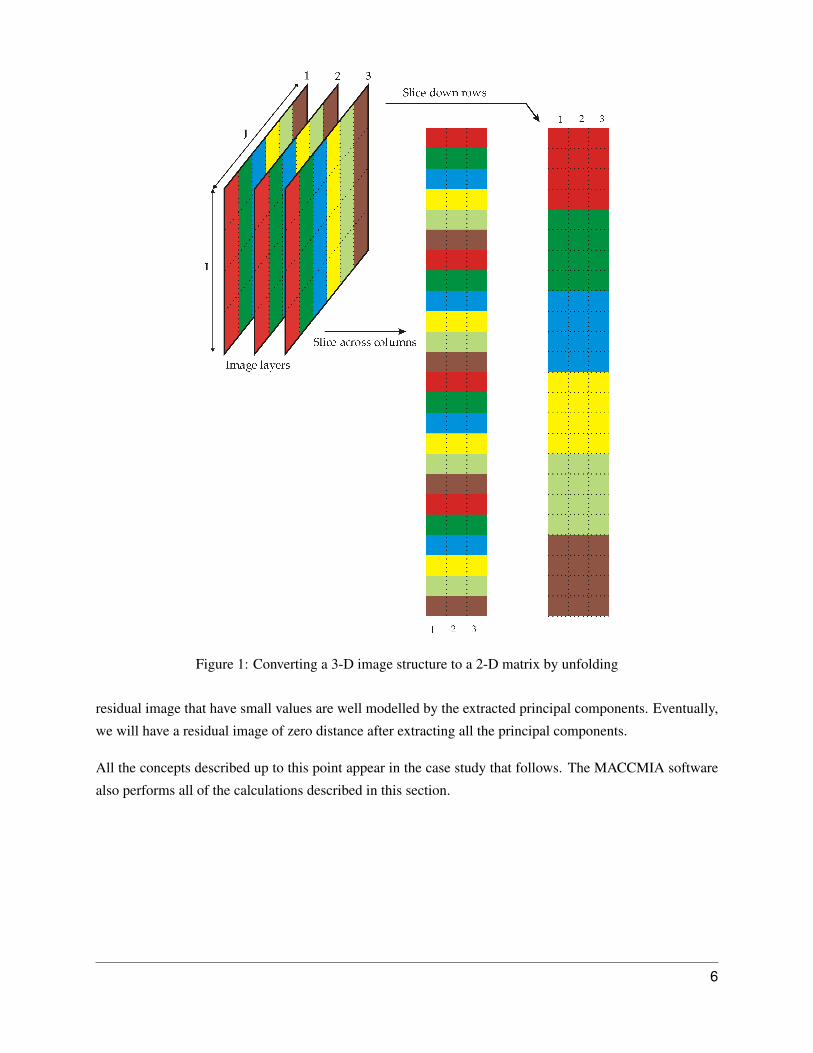
Figure 1: Converting a 3-D image structure to a 2-D matrix by unfolding

residual image that have small values are well modelled by the extracted principal components. Eventually,

we will have a residual image of zero distance after extracting all the principal components.

All the concepts described up to this point appear in the case study that follows. The MACCMIA software

also performs all of the calculations described in this section.

6

3 Installation

The current version of MACCMIA only requires Matlab. None of the Matlab toolboxes are required, in

particular, the image processing toolbox is not required, as MACCMIA does not perform “traditional” image

processing operations on the images.

MACCMIA works in both Linux and Windows. The files provided should be copied to a directory or folder

on your hard drive. For example, in Windows: C:\MACCMIA or in Linux: /home/username/maccmia/.

You may chose any other directory, but all remaining instructions in this manual will assume the directory

names used here.

Start Matlab and go to the directory where the software was installed. Type maccmia at the Matlab com-

mand line to start the software.

Please contact MACC if you experience any problems regarding the installation – see Section 6 for contact

details.

4 Tutorial case study

This section presents a tutorial-like case study illustrating how information is extracted from a satellite

image. The image is a Landsat image of Mobile, Alabama and the surrounding area. It consists of four

channels with 512 by 512 pixels per channel. The channels are of different wavelength ranges:

1. 500 to 600 nm (yellow/green)

2. 600 to 700 nm (orange/red)

3. 700 to 800 nm (deep-red/red)

4. 800 to 1100 nm (near-infrared)

Each pixel point represents an area of approximately 80 m2 on the Earth’s surface and contains a reflected

intensity value in the range 0 to 127. We could stretch out the data over the full range from 0 to 255, but this

causes no difference in the analysis.

The four channels of this image are stored in the folder C:\MACCMIA\Images\MobileALLandsat\as files called MobileAL x.tif. In order to analyze this image we need to have all the layers in a single

file. When one opens an ordinary RGB image file, such as a JPG or BMP file, the three image layers are in

the same file. The assembled image, MobileAL.mat, is provided for you already in a Matlab MAT file.

You can re–create this MAT file from the four original files by issuing the following commands in Matlab:

7

>> X = imread(’MobileAL_1.tif’); % Read layer 1

>> X(:,:,2) = imread(’MobileAL_2.tif’); % Read layer 2

>> X(:,:,3) = imread(’MobileAL_3.tif’); % Read layer 3

>> X(:,:,4) = imread(’MobileAL_4.tif’); % Read layer 4

>> save MobileAL.mat X

This MAT file now contains a single variable called X which is a 512 × 512 × 4 array, just over 1 million

data points.

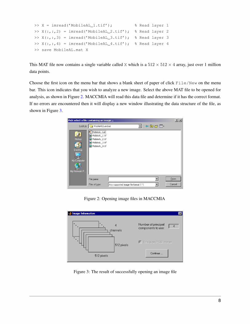
Choose the first icon on the menu bar that shows a blank sheet of paper of click File/New on the menu

bar. This icon indicates that you wish to analyze a new image. Select the above MAT file to be opened for

analysis, as shown in Figure 2. MACCMIA will read this data file and determine if it has the correct format.

If no errors are encountered then it will display a new window illustrating the data structure of the file, as

shown in Figure 3.

Figure 2: Opening image files in MACCMIA

Figure 3: The result of successfully opening an image file

8

The left part of Figure 3 allows one to check that the data has been read as intended with the correct number

of pixels in each row, column and channel. The right hand side of this figure contains information regarding

the number of principal components to use for analysis. This number is not too critical but it is recommended

that one does not choose more that 10 principal components (for memory storage considerations).

The user also has the option to confirm if the image is an RGB image. This option is disabled with images

that do not have 3 channels. If the option is left on then the true colour image is displayed for model building.

If it is turned off, then the image is displayed as a composite colour image made up from the score images.

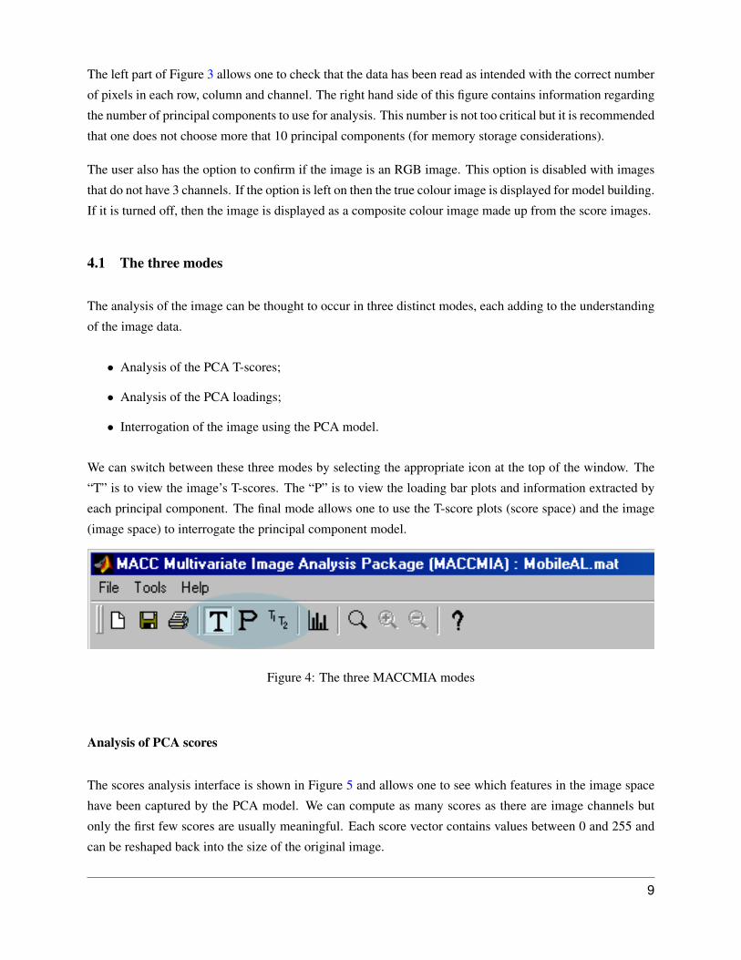
4.1 The three modes

The analysis of the image can be thought to occur in three distinct modes, each adding to the understanding

of the image data.

• Analysis of the PCA T-scores;

• Analysis of the PCA loadings;

• Interrogation of the image using the PCA model.

We can switch between these three modes by selecting the appropriate icon at the top of the window. The

“T” is to view the image’s T-scores. The “P” is to view the loading bar plots and information extracted by

each principal component. The final mode allows one to use the T-score plots (score space) and the image

(image space) to interrogate the principal component model.

Figure 4: The three MACCMIA modes

Analysis of PCA scores

The scores analysis interface is shown in Figure 5 and allows one to see which features in the image space

have been captured by the PCA model. We can compute as many scores as there are image channels but

only the first few scores are usually meaningful. Each score vector contains values between 0 and 255 and

can be reshaped back into the size of the original image.

9

Figure 5: The scores analysis interface in MACCMIA

All score vectors have values between 0 and 255, that is they are just gray–scale images that are quite

difficult to interpret. We assign a unique colour to each value in the range from 0 to 255 to interpret these

individual scores more easily and to display them as images. This is what is shown on the right hand side of

Figure 5 together with the colour mapping that is used (the jet colourmap in Matlab).

The left hand side of Figure 5 shows the image space and it appears either as a true colour RGB image or

as a multi-channel image (a false–colour composite), allowing us to compare it to the score space on the

right. The Landsat image in MACCMIA has four channels, so the concept of a “colour–image” does not

exist, but we obtain a false–colour image when we overlay any three principal component score images over

each other, assigning either Red, Green, or Blue to different score numbers. Sometimes a different colour

association can lead to a better visual understanding and reveal aspects which are not immediately apparent

when using the default assignment of:

Red = T1 Green = T2 Blue = T3

10

Assigning the three colours to the same score value will show that score as a gray-scale image.

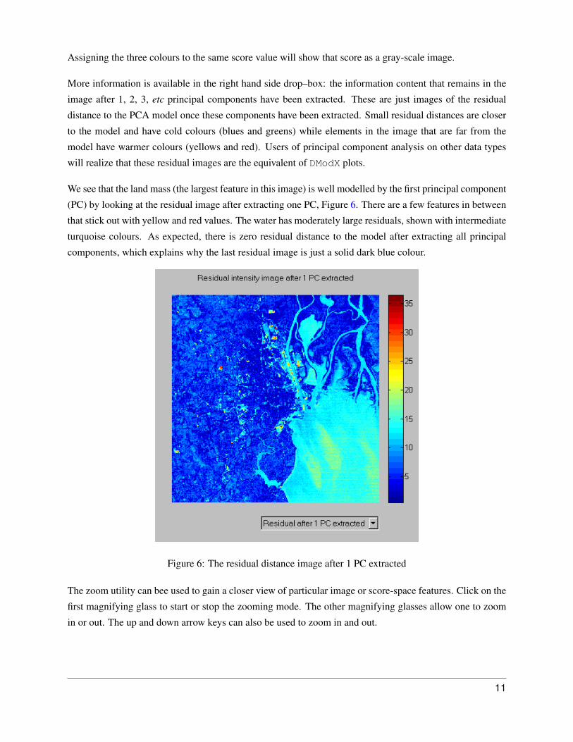
More information is available in the right hand side drop–box: the information content that remains in the

image after 1, 2, 3, etc principal components have been extracted. These are just images of the residual

distance to the PCA model once these components have been extracted. Small residual distances are closer

to the model and have cold colours (blues and greens) while elements in the image that are far from the

model have warmer colours (yellows and red). Users of principal component analysis on other data types

will realize that these residual images are the equivalent of DModX plots.

We see that the land mass (the largest feature in this image) is well modelled by the first principal component

(PC) by looking at the residual image after extracting one PC, Figure 6. There are a few features in between

that stick out with yellow and red values. The water has moderately large residuals, shown with intermediate

turquoise colours. As expected, there is zero residual distance to the model after extracting all principal

components, which explains why the last residual image is just a solid dark blue colour.

Figure 6: The residual distance image after 1 PC extracted

The zoom utility can bee used to gain a closer view of particular image or score-space features. Click on the

first magnifying glass to start or stop the zooming mode. The other magnifying glasses allow one to zoom

in or out. The up and down arrow keys can also be used to zoom in and out.

11

Analysis of PCA loadings

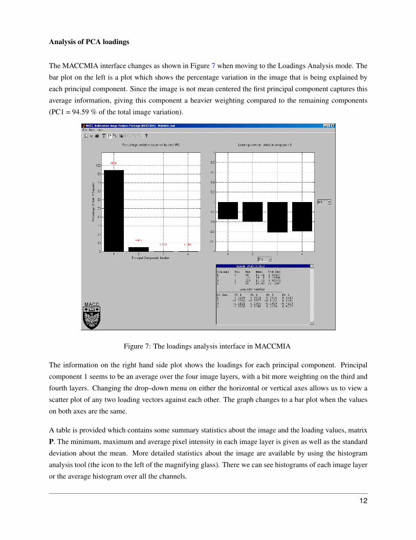
The MACCMIA interface changes as shown in Figure 7 when moving to the Loadings Analysis mode. The

bar plot on the left is a plot which shows the percentage variation in the image that is being explained by

each principal component. Since the image is not mean centered the first principal component captures this

average information, giving this component a heavier weighting compared to the remaining components

(PC1 = 94.59 % of the total image variation).

Figure 7: The loadings analysis interface in MACCMIA

The information on the right hand side plot shows the loadings for each principal component. Principal

component 1 seems to be an average over the four image layers, with a bit more weighting on the third and

fourth layers. Changing the drop–down menu on either the horizontal or vertical axes allows us to view a

scatter plot of any two loading vectors against each other. The graph changes to a bar plot when the values

on both axes are the same.

A table is provided which contains some summary statistics about the image and the loading values, matrix

P. The minimum, maximum and average pixel intensity in each image layer is given as well as the standard

deviation about the mean. More detailed statistics about the image are available by using the histogram

analysis tool (the icon to the left of the magnifying glass). There we can see histograms of each image layer

or the average histogram over all the channels.

12

Since the mean is not subtracted from each image we often find that the mean value in each layer is propor-

tional to the value of P1 for that layer. This is not a fixed rule, but rather explains the interpretation of the

first principal component as being a single “average” image over all the image layers.

Layer P1 Mean

1 −0.3455 13.04

2 −0.3943 14.18

3 −0.6121 19.92

4 −0.5920 18.43

Image and model interrogation mode

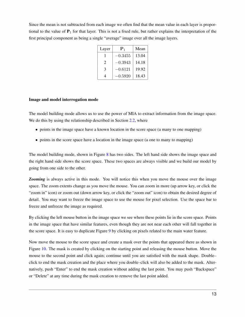
The model building mode allows us to use the power of MIA to extract information from the image space.

We do this by using the relationship described in Section 2.2, where

• points in the image space have a known location in the score space (a many to one mapping)

• points in the score space have a location in the image space (a one to many to mapping)

The model building mode, shown in Figure 8 has two sides. The left hand side shows the image space and

the right hand side shows the score space. These two spaces are always visible and we build our model by

going from one side to the other.

Zooming is always active in this mode. You will notice this when you move the mouse over the image

space. The zoom extents change as you move the mouse. You can zoom in more (up arrow key, or click the

“zoom in” icon) or zoom out (down arrow key, or click the “zoom out” icon) to obtain the desired degree of

detail. You may want to freeze the image space to use the mouse for pixel selection. Use the space bar to

freeze and unfreeze the image as required.

By clicking the left mouse button in the image space we see where these points lie in the score space. Points

in the image space that have similar features, even though they are not near each other will fall together in

the score space. It is easy to duplicate Figure 9 by clicking on pixels related to the main water feature.

Now move the mouse to the score space and create a mask over the points that appeared there as shown in

Figure 10. The mask is created by clicking on the starting point and releasing the mouse button. Move the

mouse to the second point and click again; continue until you are satisfied with the mask shape. Double–

click to end the mask creation and the place where you double–click will also be added to the mask. Alter-

natively, push “Enter” to end the mask creation without adding the last point. You may push “Backspace”

or “Delete” at any time during the mask creation to remove the last point added.

13

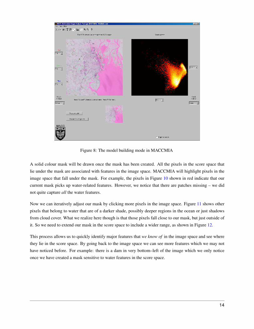
Figure 8: The model building mode in MACCMIA

A solid colour mask will be drawn once the mask has been created. All the pixels in the score space that

lie under the mask are associated with features in the image space. MACCMIA will highlight pixels in the

image space that fall under the mask. For example, the pixels in Figure 10 shown in red indicate that our

current mask picks up water-related features. However, we notice that there are patches missing – we did

not quite capture all the water features.

Now we can iteratively adjust our mask by clicking more pixels in the image space. Figure 11 shows other

pixels that belong to water that are of a darker shade, possibly deeper regions in the ocean or just shadows

from cloud cover. What we realize here though is that those pixels fall close to our mask, but just outside of

it. So we need to extend our mask in the score space to include a wider range, as shown in Figure 12.

This process allows us to quickly identify major features that we know of in the image space and see where

they lie in the score space. By going back to the image space we can see more features which we may not

have noticed before. For example: there is a dam in very bottom–left of the image which we only notice

once we have created a mask sensitive to water features in the score space.

14

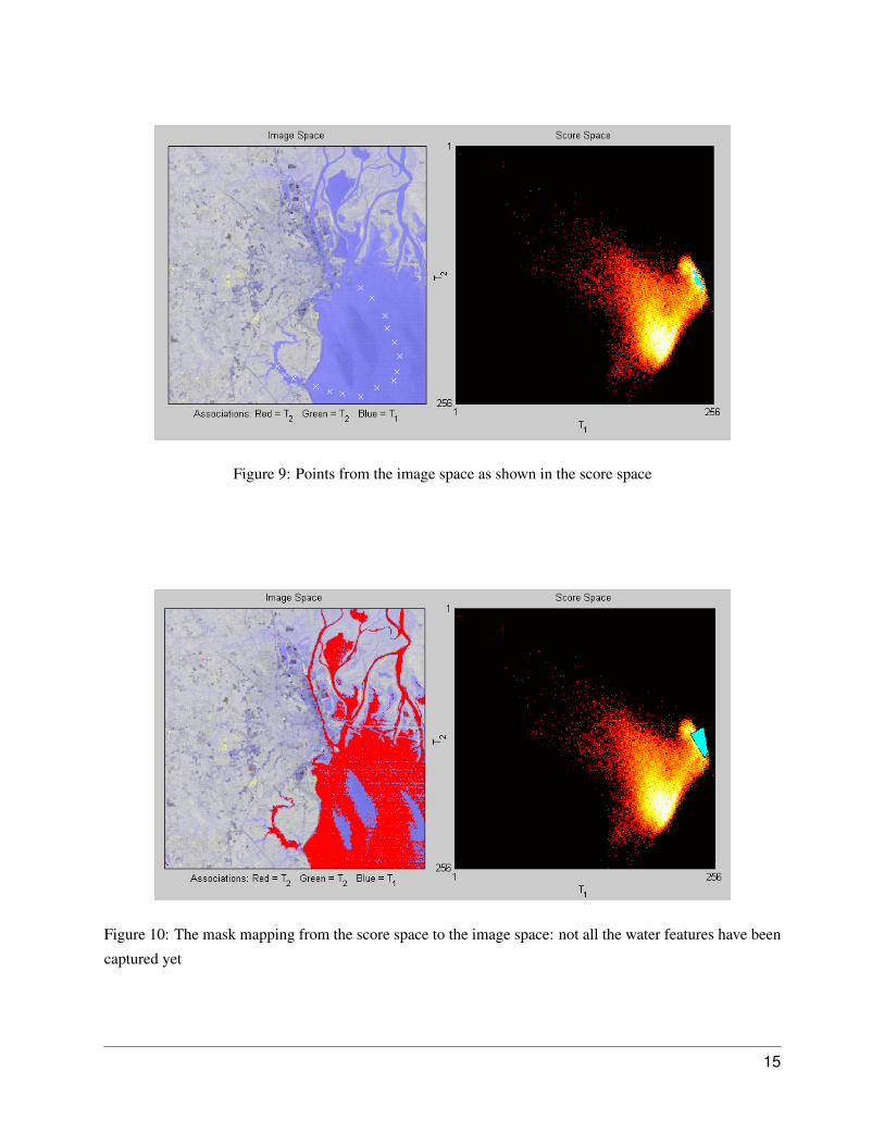
Figure 9: Points from the image space as shown in the score space

Figure 10: The mask mapping from the score space to the image space: not all the water features have been

captured yet

15

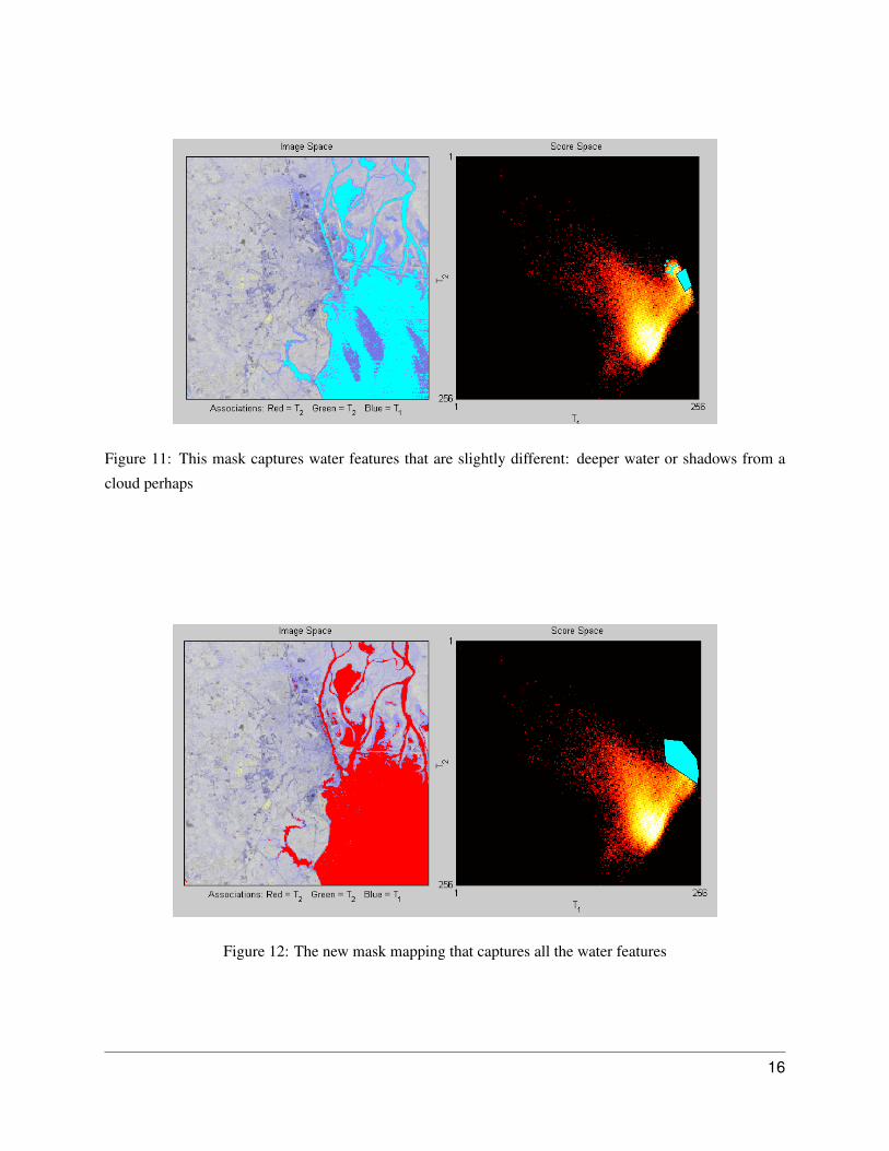
Figure 11: This mask captures water features that are slightly different: deeper water or shadows from a

cloud perhaps

Figure 12: The new mask mapping that captures all the water features

16

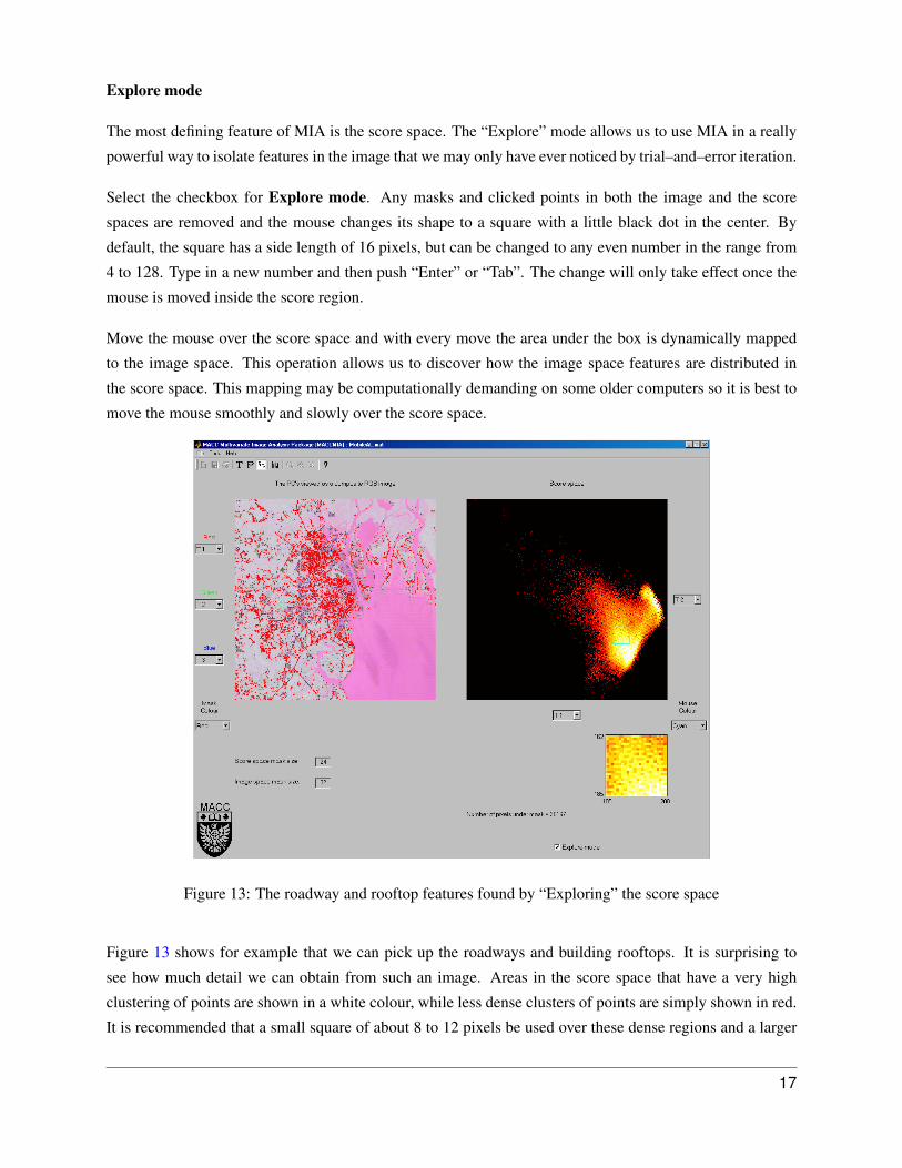
Explore mode

The most defining feature of MIA is the score space. The “Explore” mode allows us to use MIA in a really

powerful way to isolate features in the image that we may only have ever noticed by trial–and–error iteration.

Select the checkbox for Explore mode. Any masks and clicked points in both the image and the score

spaces are removed and the mouse changes its shape to a square with a little black dot in the center. By

default, the square has a side length of 16 pixels, but can be changed to any even number in the range from

4 to 128. Type in a new number and then push “Enter” or “Tab”. The change will only take effect once the

mouse is moved inside the score region.

Move the mouse over the score space and with every move the area under the box is dynamically mapped

to the image space. This operation allows us to discover how the image space features are distributed in

the score space. This mapping may be computationally demanding on some older computers so it is best to

move the mouse smoothly and slowly over the score space.

Figure 13: The roadway and rooftop features found by “Exploring” the score space

Figure 13 shows for example that we can pick up the roadways and building rooftops. It is surprising to

see how much detail we can obtain from such an image. Areas in the score space that have a very high

clustering of points are shown in a white colour, while less dense clusters of points are simply shown in red.

It is recommended that a small square of about 8 to 12 pixels be used over these dense regions and a larger

17

size square over regions with more sparse clustering.

The same principle is applied in reverse when moving the mouse over the image space. The corresponding

score space points are dynamically highlighted.

4.2 Further examples

A far more complete description of MIA appears in the book by Geladi and Grahn [1996]. The satellite

image is used as an example in that book together with a variety of other interesting images. The book

contains detailed Matlab code for performing the all the basic operations of MIA, such as computing the

principal components, the loadings, the score images, the score space and the residual images.

The Landsat image of Mobile, Alabama appeared in the paper by Geladi and Esbensen [1991]. The final part

of that paper shows how MIA may be extended to regression problems, that is to predict variable(s) using

an image as the predictor block. The Landsat image was also used in the paper by Bharati and MacGregor

[1998]. Their paper shows how the masks in the score space can be used for monitoring changes in multiple

image space features, in real–time.

The score images in the papers by Geladi and Esbensen [1991] and Bharati and MacGregor [1998] look

slightly different to those obtained by MACCMIA because a different singular value decomposition algo-

rithm was used. These differences cause opposite signs on some of the principal components, which make

the score space images appear as reflected versions of the MACCMIA output. The phenomenon happens

quite frequently in PCA but does not provided any trouble or incorrect answers, provided we work consis-

tently.

Finally, an RGB image of a piece of lumber that was used in the paper by Bharati et al. [2003] is also

provided as part of the MACCMIA package. This image shows how irregular features such as splits and

knots that appear in different locations on the piece of lumber are grouped together in one place in the score

space. This technique can be used for real–time monitoring of lumber production.

4.3 Printing and saving

Printing and saving figures in MACCMIA is accomplished by right–clicking on any plot. In the Scores

Analysis and Loadings Analysis mode there will only be one option: “Send this axis to a new figure win-

dow”. A new figure window will open containing the image or plot that the original axis contained. Titles

and axis labelling are also included, where applicable. One can further manipulate the image in this figure

window by adding different titles and labelling. This new figure window also allows one to copy the image

to the clipboard for pasting in other programs, to print the image or save it to disk as a Matlab FIG file.

18

An additional option is available in the model building mode when right–clicking on either the image or the

score space: “Send both image and score space to a new figure window”. This option will place the image

and score space in a single window, side-by-side.

The data used by MACCMIA can also be saved to a Matlab MAT file. One is prompted for a new file name

when selecting File/Save from the menu (or just push Ctrl-S). MACCMIA will save all the relevant details

accumulated during the analysis of a particular image to this file. This file will contain a single structured

variable called MACCMIA as shown in the table below. Future versions of MACCMIA will allow one to

open this file and continue the analysis of the image from where you left off.

Field name Description Size/ContentsVersion The version number used to generate the file string

Image.Filename The file and directory containing the image char array

Image.nRows The number of pixel rows in the original image integer

Image.nCols The number of pixel columns in the original image integer

Image.nLayers The number of layers in the original image integer

Image.cdata The original image data 3–D array

PCAmodel.numPC The number of principal components used in the model integer

PCAmodel.Loadings The loading matrix with p1 down the first column, etc square matrix

PCAmodel.Eigenvalues The eigenvalues along the diagonal of a square matrix square matrix

PCAmodel.Tmin The minimum score value calculated (for rescaling) vector

PCAmodel.Tmax The maximum score value calculated (for rescaling) vector

.TScoresAsImages The scores, as images, scaled with min and max vectors 3–D array, uint8

ScoreSpace.ColourMap The colour map used to display the score images 256× 3 array

ScoreSpace.Mask A 0/1 image, with 1’s inside the mask 256 by 256

ScoreSpace.Xpoints The x–axis coordinate of the mask vertices vector

ScoreSpace.Ypoints The y–axis coordinate of the mask vertices vector

19

5 How to analyze your own images

To understand the rest of this section it is necessary to take a brief diversion and understand some imaging

concepts and how images are treated in Matlab.

5.1 Image dimensions

Matlab is capable of reading different image file formats using its imread.m function. The following

formats are currently supported: TIFF, PNG, HDF, BMP, JPEG, PCX, XWD, CUR, ICO. This

command is used in Matlab in the following manner:

>> X = imread(’MyPicture.jpg’); % This puts the JPEG image into array X

If the file ’MyPicture.jpg’ contained a colour image that was “640 by 480” pixels, then Matlab will

create a matrix X to be of size 480x640x3. It is unfortunate that images are often read with the width (the

number of columns) first and then the height (the rows) (eg: a 640 by 480 image), but in mathematics it is

standard to first report the number of rows and then the number of columns.

A word of caution is necessary from the very beginning on image representation:

One should be careful not to directly associate the first two dimensions to the rows and columns

of a matrix. The first number (640) refers to the number of columns in the image (going from

left to right, across the rows). The second number (480) refers to the number of rows in the

image (going from top to bottom, down the columns).

In this guide we will refer to the image array as X, indicating that it is not a two–dimensional matrix, but a

three–dimensional array.

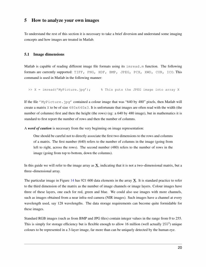
The particular image in Figure 14 has 921 600 data elements in the array X. It is standard practice to refer

to the third dimension of the matrix as the number of image channels or image layers. Colour images have

three of these layers, one each for red, green and blue. We could also use images with more channels,

such as images obtained from a near infra–red camera (NIR images). Such images have a channel at every

wavelength used, say 128 wavelengths. The data storage requirements can become quite formidable for

these images.

Standard RGB images (such as from BMP and JPG files) contain integer values in the range from 0 to 255.

This is simply for storage efficiency but is flexible enough to allow 16 million (well actually 2553) unique

colours to be represented in a 3-layer image, far more than can be uniquely detected by the human eye.

20

Figure 14: The data structure of ordinary colour images

5.2 Preparing images for use in MACCMIA

MACCMIA can analyze most images without any user intervention: MACCMIA will attempt to open the

image file directly using Matlab’s imread.m function. If that does not succeed, then it will just load the

data and see if it is in the form of an image. If MACCMIA cannot open the file correctly then an error

message will be provided with further information. If you have created an image by other means (maybe

from a wavelet analysis or you are using data from an NIR camera), then MACCMIA can still analyze the

data if the ‘image’ obeys the following rules:

• the image is of type uint8 or double;

• the image has three or more layers on which the multivariate analysis will be performed;

• the image is stored in a Matlab MAT file either by itself or with other variables (MACCMIA will

prompt the user to select the variable to load).

6 Technical support

Technical support of the software is provided to MACC member companies as part of the software package.

Feel free to contact the appropriate person by email or telephone regarding any queries that you may have.

Suggestions for new features and improvements to the software are very welcome.

Contacts: Kevin Dunn (905) 528 9136 kevin.dunn@prosensus.ca Technical

Dr. John MacGregor (905) 525 9140 × 24951 macgreg@mcmaster.ca Administration

21

References

BHARATI, M. H. AND MACGREGOR, J. F. (1998). Multivariate Image Analysis for Real–Time Process

Monitoring and Control. Industrial and Engineering Chemistry Research, 37, 4715–4724.

BHARATI, M. H., MACGREGOR, J. F., AND TROPPER, W. (2003). Softwood Lumber Grading through

On-line Multivariate Image Analysis Techniques. Industrial and Engineering Chemistry Research, 42,

5345–5353.

GELADI, P. AND ESBENSEN, K. (1991). Multivariate Image Analysis in Chemistry: An Overview. In

Devilliers, J. and Karcher, W. (Eds.), Applied Multivariate Analysis in SAR and Environmental Studies,

pp. 415–445. Kluwer Academic Publishers.

GELADI, P. AND GRAHN, H. (1996). Multivariate Image Analysis. John Wiley and Sons.

22