Embed Size (px)
Citation preview

MACAW: A Media Access Protocol for Wireless LAN’s
Vaduvur Bharghavan
Department of Electrical Engineering and Computer Science
University of California at Berkeley
[email protected]. edu
Alan Demers Scott Shenker Lixia Zhang
Palo Alto Research Center
Xerox Corporation
{demers, shenker, lixia}@parc.xerox. com
Abstract
In recent years, a wide variety of mobile computing devices
has emerged, including portables, palmtops, and personal
digit al assistants. Providing adequate network connectivity y
for these devices will require a new generation of wireless
LAN technology. In this paper we study media access pro-
tocols for a single channel wireless LAN being developed at
Xerox Corporation’s Palo Alto Research Center. We start
with the MACA media access protocol first proposed by
Karn [9] and later refined by Biba [3] which uses an RTS-
CTS-DATA packet exchange and binary exponential back-
off. Using packet-level simulations, we examine various per-
formance and design issues in such protocols, Our analysis
leads to a new protocol, MACAW, which uses an RTS-CTS-
DS-DATA-ACK message exchange and includes a signifi-
cantly different backoff algorithm.
1 Introduction
In recent years, a wide variety of mobile computing devices
have emerged, including palmtops, personal digital assis-
tants, and portable computers. While the first portables
were designed as stand-alone machines, many of these new
devices are intended to function as full network citizens.
Consequently, a new generation of wireless network technol-
ogy is needed to provide adequate network cormectivitY for
these mobile devices. In particular, wireless local area net-
works (LAN’s) are expected to be a crucial enabling technol-
ogy in traditional office settings where such mobile devices
will be initially, and most heavily, utilized.
The media in a wireless network is a shared, and scarce,
resource; thus one of the key questions is how access to this
shared media is controlled. In this paper, we focus on media
access protocols in wireless LAN’s. Our research has a dual
purpose. One goal is to develop a media access protocol for
use in the wireless network infrastructure being developed
in the Computer Science Laboratory at Xerox Corporation’s
Palo Alto Research Center [7, 8]. The other goal is to explore
some of the basic performance and design issues inherent in
wireless media access protocols. While our specific simu-
Permission to copy without fee all or part of this material isgranted provided that the copies are not made or distributed fordirect commercial advantage, the ACM copyright notice and thetitle of the publication and its date appear, and notice is given
lation results may only apply to PARC’s particular radio
technology, we expect that some of the basic insight gained
will be more generally applicable.
Wireless media access protocols for a single channel can
typically be categorized as either token-based or multiple ac-
cess. For reasons we explain in the next section, we choose
the multiple access approach. 1 Our work is based on MACA,
a Multiple Access, Collision Avoidance protocol first pro-
posed by Karn [9] and later refined by Biba [3]. Using
packet-level simulations of the wireless network to guide our
design, we suggest several modifications to MACA. We call
the resulting algorithm MACAW, in recognition of its ge-
nealogical roots in Karn’s original proposal Our design is
based on four key observations. First we observe, follow-
ing Karn [9] and others [4, 12], that the relevant contention
is at the receiver, not the sender. This renders the car-
rier sense approach inappropriate. Second, we note that,
in contrast to Ethernets, congestion is location dependent;
in fact, the first observation is irrelevant wit bout the sec-
ond. Third, we conclude that, to allocate media access fairly,
learning about congestion levels must be a collective enter-
prise. That is, the media access protocol should propagate
congestion information explicitly rather than having each
device learn about congestion independently. Fourth, the
media access protocol should propagate synchronize ation in-
formation about contention periods, so that all devices can
cent end effectively. In particular, this means that cent ention
for bandwidth should not just be initiated by the sending
device. While our proposed protocol provides enhanced per-
formance (as compared to MACA), we hasten to note that
it is merely an initial attempt to deal with these challenges;
there are many remaining unresolved design issues.
This paper has 5 sections. In Section 2 we first pro-
vide some background on PARC’s radio network and on the
MACA media access protocol. We then, in Section 3, discuss
our modifications to MACA; we motivate these changes by
presenting simulation data for several different network con-
figurations. We discuss remaining design issues in Section 4
and summarize our findings in Section 5.
1 We expect in future work to revisit the token-based approach and
make a more in-depth comparison.
that copying is by permission of the Association of ComputingMachinery. To copy otherwise, or to republish, requires a feeand/or specific permission.SIGCOMM 94 -8/94 London England UK@ 1994 ACM 0-89791 -682 -4/94/0008 ..S3.50
212

2 Background
2.1 PARC’s Nano-Cellular Radio Network
The Computer Science Laboratory at Xerox Corporation’s
Palo Alto Research Center has developed 5 MHz “near-field”
radio t ethnology [7]; its low operating frequency eliminates
multipath effects, and thus it is suitable for use in an indoor
wireless LAN. The LAN infrastructure consists of “base sta-
tions”, which are installed in the ceiling, and “pads”, which
are custom built portable computing devices (see [8] for a
more complete description). There is a single 256kbps chan-
nel, and all wireless communication is between a pad and a
base station (the base stations are connected together by an
Ethernet). All base stations and pads transmit at the same
signal strength. The range of transmission is 3 to 4 me-
ters, and the near-field signal strength decays very rapidly
(X .-3, as opposed tow r-’ in the far-field region). We thus
obtain, around each base station, a very small cell (roughly
6 meters in diameter) with very sharply defined boundaries:
a “nanocell”. Given that the cells are very small and inter-
cell interference is negligible, the aggregate bandwidth in a
multi-cell environment is quite high.
A “collision” occurs when a receiver is in the reception
range of two transmitting stations2, and is unable to cleanly
receive signal from either station. “Capture” occurs when
a receiver is in the reception range of two transmitting sta-
tions, but is able to cleanly receive signal from the closer
station; this can only occur if the signal power ratio is large
(w 10db or more). This requires a distance ratio of x 1.5.Perhaps surprisingly, this ratio is rather hard to achieve,
given that the base stations are in the ceiling and the pads
are typically no higher than a meter or so above the floor.
Roughly, this gives a minimum pad-to-base distance of just
under 2 meters in a cell whose radius is just over 3 meters.
Thus, in our environment, capture will be relatively rare,
and is not a primary design consideration.
“Interference” occurs when a receiver is in range of one
transmitting station and slightly out-of-range of another
transmitting station, but is unable to cleanly receive the
closer station’s signal because of the interfering presence of
the other signal. The rather sharp decay in signal strength
makes interference rather rare in our environment, and we
do not make it a major factor in our design.
Ignoring both capture and interference leads to a very
simple model in which any two stations are either in-range
or out-of-range of one another, and a station successfully
receives a packet if and only if there is exactly one active
transmitter within range of it. In designing our protocol,
we often use this model accompanied by the additional ass-
umptions that no two base stations are within range of each
other, and that no pad is within range of two different base
stations. This is an extremely poor model for far-field ra-
dios. It is not quite so poor for our near-field radios, but it
is still far from realistic. We have not used this naive model
in any of our simulations, but we do use it for intuitive jus-
tification of some of the algorithms given below.
Controlling access to a shared media is much easier if
the locations of the various devices are known. However.
in our setting there is no independent source of location
information for the pads. There is no way for a pad to know
that it is leaving a cell except through the loss of signal from
the baae station. Furthermore, there is no way for a pad,
‘We will use the term stat]on to refer to both pads and base
stations.
or base station, to know about the presence of other devices
besides explicit communication.
It is important to note that, in the absence of noise, our
technology is symmetric; if a station A can hear a station B,
then station B can hear the station A. The presence of noise
sources (e.g., displays) may interfere with this symmetry,
and in our simulations we will consider the effect of noise.
However, noise is not so prevalent that we make it the over-
riding factor in our design; rather, we design our protocol
to tolerate noise well but we have done most of our testing
in a noise-free setting.
There are many different ways to control access to a sin-
gle channel. Typically, these approaches are either multiple
access or token-based. We chose the multiple access ap
preach over the token approach for two reasons.3 First,
multiple access schemes are typically more robust. This is
especially important in a wireless environment where the
mobile devices span the gamut of reliability. Second, we ex-
pect the pads to be highly mobile and, given the small cell
size, these pads will enter and leave cells frequently. This
would necessitate frequent token hand-offs or recovery in a
token-based scheme.
One common wireless multiple access algorithm, cur-
rently used in packet radio, is carrier sense (CSMA). In the
next section we discuss its properties and argue, following
Karn [9] and others [4, 12], that the CSMA approach is in-
appropriate e for our setting.
2.2 CSMA
In CSMA, every station senses the carrier before transmit-
ting; if the station detects carrier then the station defers
transmission (CSMA schemes differ as to when the trans-
mission is tried again). Carrier sense attempts to avoid col-
lisions by testing the signal strength in the vicinity of the
transmitter. However, collisions occur at the receiver, not
the transmitter; that is, it is the presence of two or more
interfering signals at the receiver that constitutes a colli-
sion. Since the receiver and the sender are typically not
co-located, carrier sense does not provide the appropriate
information for collision avoidance. Two examples illustrate
this point in more detail. Consider the configuration de-
picted in Figure 1. Station A can hear B but not C, and
station C can hear station B but not A (and, by symmetry,
we know that station B can hear both A and C).
(xJ @J)@)Figure 1: Station B can hear both A and C, but A and C
cannot hear each other. A “hidden terminal” scenario re-
sults when C attempts to transmit while A is transmitting
to B. An ‘exposed terminal” scenario results if B is trans-
mitting to A when C attempts to transmit.
First, assume A is sending to B. When C is ready to
transmit (perhaps to B or perhaps to some other station),
it does not detect carrier and thus commences transmission;
this produces a collision at B. Station C’s carrier sense did
not provide the necessary information since station A was
3 These ressons are merely intuitive guides for design. We hope,
in future work, to explore the token- bssed approach more fully. Onlythen can we make a vahd comparison between the two approaches.
213

“hidden” from it. This is the classic “hidden terminal” sce-
nario.
An “exposed” terminal scenario results if now we assume
that B is sending to A rather than A sending to B. Then,
when C is ready to transmit, it does detect carrier and there-
fore defers transmission. However, there is no reason to de-
fer transmission to a station other than B since station A is
out of C’s range (and, as we stated earlier, in our environ-
ment there are no “interference effects” from out-of-range
stations). Station C‘s carrier sense did not provide the nec-
essary information since it was exposed to station B even
though it would not collide or interfere with B’s transmis-
sion.
Carrier sense provides information about potential colli-
sions at the sender, but not at the receiver. This information
can be misleading when the configuration is distributed so
that not all stations are within range of each other. Because
carrier sense does not provide the relevant collision avoid-
ance information, we chose to seek another approach based
on MACA, which we describe below.
2.3 MACA
Karn proposed MACA for use in packet radio as an alter-
native to the traditional CSMA media access scheme [9].
MACA is somewhat similar to the protocol proposed in [3]
and also to that used in WaveLAN, and both resemble the
basic Apple LocalTalk Link Access Protocol [2]. Here we
present a very brief and general description of the algorithm
([9] is itself a brief description and does not specify many
details).
MACA uses two types of short, fixed-size signaling pack-
ets. When station A wishes to transmit to station B, it sends
a Request-to-Send (RTS) packet to B; this RTS packet con-
t ains the length of the proposed data transmission. If station
B hears the RTS, and it is not currently deferring (which we
explain below), it immediately replies with a Clear-to-Send
(CTS) packet; this CTS also contains the length of the pro-
posed data transmission. Upon receiving the CTS, st ation A
immediately sends its data. Any station overhearing an RTS
defers all transmissions until some time after the associated
CTS packet would have finished (this includes the time for
transmission of the CTS packet as well as the “turnaround”
time at the receiving st ation4 ). Any station overhearing
a CTS packet defers for the length of the expected data
transmission (which is contained in both the RTS and CTS
packets).
With this algorithm, any station hearing an RTS will
defer long enough so that the transmitting station can re-
ceive the returning CTS. Any station hearing the CTS will
avoid colliding wit h the returning data transmission. Since
the CTS is sent from the receiver, symmetry assures us that
every station capable of colliding with the data transmission
is in range of the CTS (it is possible, though, that the CTS
may not be received by all in-range stations due to other
transmissions in the area). Notice that stations that hear
an RTS but not a CTS because they are in range of the
sender but out of range of the receiver can commence trans-
mission, without harm, after the CTS has been sent; since
they are not in range of the receiver they cannot collide with
the data transmission.
4 This turnaround time is the time from the reception of the RTS
at the receiving antenna to the transmission of the CTS; this includes
operating system delays as well as radio transients.
In the hidden terminal scenario in Figure I, station C
would not hear the RTS from station A, but would hear the
CTS from station B and therefore would defer from trans-
mit ting during A’s data transmission. In the exposed t ermi-
rral scenario, station C would hear the RTS from station B,
but not the CTS from station A, and thus would be free to
transmit during B’s data transmission. This is exactly the
desired behavior.
Thus, in contrast to carrier-sense, this RTS-CTS ex-
change enables nearby stations to avoid collisions at the
receiver, not the sender. The role of the RTS is to elicit
from the receiver the CTS, whose reception can be used by
other stations as an indication that they are in range and
thus could collide with the impending transmission. This
depends crucially on symmetry; if a station cannot hear sta-
tion B’s CTS then we assume that that station cannot colhde
with an incoming transmission to B.
If station A does not hear a CTS in response from station
B, it will eventually time out (i. e., stop waiting), assume a
collision occurred, and then schedule the packet for retrans-
mission. MACA uses the binary exponential backoff (BEB)
algorithm to select this retransmission time.
3 Designing MACAW
Our purpose here is to re-evaluate some of the basic design
choices in MACA and then produce a revised version suit-
able for use in PARC’s wireless LAN. The MACA algorithm,
as p~esented in [9], is a preliminary design and leaves many
detads unspecified. We start our investigation by defining
these details for an initial version. Appendix A gives the
pseudo-code we used to implement MACA.
We mention several aspects of this algorithm here. First,
the control packets (RTS, CTS) are 30 bytes long. The
transmission time of these packets defines the ‘slot” time
for retransmissions. Retransmissions occur if and only if a
station does not receive a CTS in response to its RTS. Re-
transmission are scheduled an integer number of slot times
after the end of the last deferral period. A station ran-
domly chooses, with uniform distribution, this integer be-
tween 1 and BO, where BO represents the backoff counter.
The backoff algorithm adjusts the value of BO through two
functions, Fdec and F,m.. Whenever a CTS is received af-
ter an RTS, the backoff counter is adjusted via the function
Fd~d BO := F~~c(~O). Whenever a CTS is not received af-
ter an RTS, the backoff counter is adjusted via the function
F tnc: BO := F,. C(BO). For BEB, Fd.c(z) = BO~,~ and
F,nc(s) = MIN[2z, BO ] hmaz , w ere BOmin and BOmaz rep-
resent the lower and upper bounds for the backoff counter,
respectively. For our simulations we have chosen BOm,n = 2and BOma. = 64.
We use packet-level simulations of the protocol to evalu-
ate our design decisions. The simulator we use is a modifi-
cation of the network simulator we have used in a number of
other studies (for example, [5]) of wired networks. The simu-lator is event-driven and contains the following components:
a traffic generator (which can generate data streams accord-
ing to various statistical models), TCP, UDP, 1P, pads, and
base stations. The simulator approximates the media by di-
viding the space into small cubes and then computing the
strength of a signal at each cube according to the distance
from the signal source to the center of the cube. Errors due
to the cube approach can be made arbitrarily small by re-
ducing the cube size. For the simulations mentioned in this
214
base station
B
/?
oPI o
P2
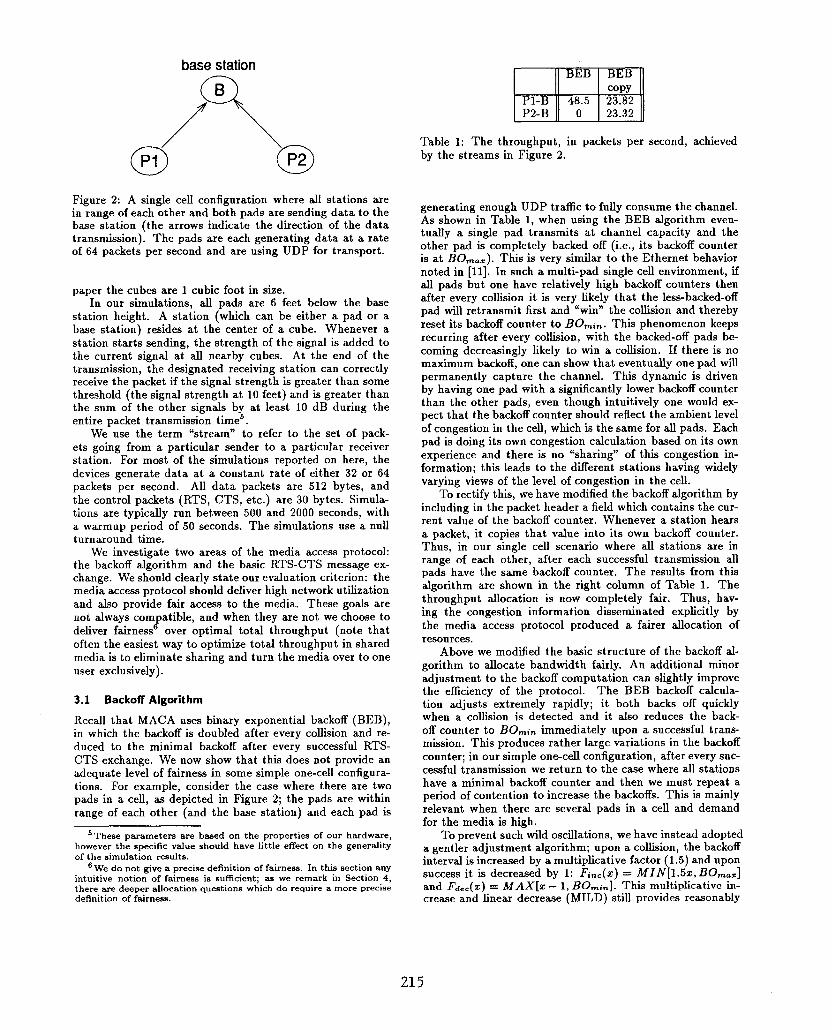
Figure 2: A single celI configuration where all stations are
in range of each other and both pads are sending data to the
base station (the arrows indicate the direction of the data
transmission). The pads are each generating data at a rate
of 64 packets per second and are using U DP for transport.
paper the cubes are 1 cubic foot in size.
In our simulations, all pads are 6 feet below the base
station height. A station (which can be either a pad or a
base station) resides at the center of a cube. Whenever a
station start& sending, the strength of the signal is added to
the current signal at all nearby cubes. At the end of the
transmission, the designated receiving station can correctly
receive the packet if the signal strength is greater than some
threshold (the signal strength at 10 feet) and is greater than
the sum of the other signals by at least 10 dB during the
entire packet transmission times.
We use the term “stream” to refer to the set of pack-
ets going from a particular sender to a particular receiver
station. For most of the simulations reported on here, the
devices generate data at a constant rate of either 32 or 64
packets per second. All data packets are 512 bytes, and
the control packets (RTS, CTS, etc.) are 30 bytes. Simula-
tions are typically run between 500 and 2000 seconds, with
a warmup period of 50 seconds. The simulations use a null
turnaround time.
We investigate two areas of the media access protocol:
the backoff algorithm and the basic RTS-CTS message ex-
change. We should clearly state our evaluation criterion: the
media access protocol should deliver high network utilization
and also provide fair access to the media. These goals are
not always compatible, and when they are not we choose to
deliver fairness6 over optimal total throughput (note that
often the easiest way to optimize total throughput in shared
media is to eliminate sharing and turn the media over to one
user exclusively).
3.1 Backoff Algorithm
Recall that MACA uses binary exponential backoff (BEB),
in which the backoff is doubled after every collision and re-
duced to the minimal backoff after every successful RTS-
CTS exchange. We now show that this does not provide an
adequate level of fairness in some simple one-cell configura-
tions. For example, consider the case where there are two
pads in a cell, as depicted in Figure 2; the pads are within
range of each other (and the base station) and each pad is
5 These parameters are based on the properties of our hardware,
however the specific value should have little effect on the generality
of the simulation results.
6 We do not give a precise definition of fairness, In this section any
intuitive notion of fairness is sufficient; ss we remark in Section 4,
there are deeper allocation questions which do require a more precise
definition of fairness.
EIEiliaTable 1: The throughput, in packets per second, achieved
by the streams in Figure 2.
generating enough UDP traffic to fully consume the channel.
As shown in Table 1, when using the BEB algorithm even-
tually a single pad transmits at channel capacity and the
other pad is completely backed off (i.e., its backoff counter
is at BOmac ). This is very similar to the Ethernet behavior
noted in [11]. In such a multi-pad single cell environment, if
all pads but one have relatively high backoff counters then
after every co~lon it is very likely that the less-backed-off
pad will retransmit first and “win” the collision and thereby
reset its backoff counter to BOrnin. This phenomenon keeps
recurring after every collision, with the backed-off pads be-
coming decreasingly likely to win a collision. If there is no
maximum backoff, one can show that eventually one pad will
permanently capture the channel. This dynamic is driven
by having one pad with a significantly lower backoff counter
than the other pads, even though intuitively one would ex-
pect that the backoff counter should reflect the ambient level
of congestion in the cell, which is the same for all pads. Each
pad is doing its own congestion calculation based on its own
experience and there is no “sharing” of this congestion in-
formation; this leads to the different stations having widely
varying views of the level of congestion in the cell.
To rectify this, we have modified the backoff algorithm by
including in the packet header a field which contains the cur-
rent value of the backoff counter. Whenever a station hears
a packet, it copies that value into its own backoff counter.
Thus, in our single cell scenario where all stations are in
range of each other, after each successful transmission all
pads have the same backoff counter. The results from this
algorithm are shown in the right column of Table 1. The
throughput allocation is now completely fair. Thus, hav-
ing the congestion information dwseminated explicitly by
the media access protocol produced a fairer allocation of
resources.
Above we modified the basic structure of the backoff al-
gorithm to allocate bandwidth fairly. An additional minor
adjustment to the backoff computation can slightly improve
the efficiency of the protocol. The BEB backoff crdcula-
tion adjusts extremely rapidly; it both backs off quickly
when a collision is detected and it also reduces the back-
OR counter to BOmin immediately upon a successful trans-
mission. This produces rather large variations in the backoff
counter; in our simple one-cell configuration, after every suc-
cessful transmission we return to the case where all stations
have a minimal backoff counter and then we must repeat a
period of contention to increase the backoffs. This is mainly
relevant when there are several pads in a cell and demand
for the media is high.
To prevent such wild oscillations, we have instead adopted
a gentler adjustment algorithm; upon a collision, the backoff
interval is increased by a multiplicative factor (1.5) and upon
success it is decreased by 1: Fine(z) = JflN[l.5z, Born..]
and Fa..(z) = MAX[Z —1, BcL+I. This rnultb~cative in-crease and linear decrease (MILD) still provides reasonably
215
base station base station
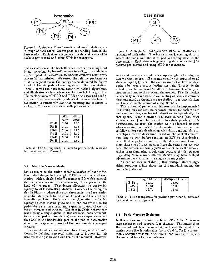
Figure 3: A single cell configuration where all stations are
in range of each other. All six pads are sending data to the
base station. Each stream is generating data at a rate of 32
packets per second and using UDP for transport.
quick escalation in the backoffs when contention is high but
by not resetting the backoff counter to BOm,n it avoids hav-
ing to repeat the escalation in backoff counters after every
successful transmission. We tested the relative performance
of these algorithms in the configuration depicted in Figure
3, which has six pads all sending data to the base station.
Table 2 shows the data from these two backoff algorithms,
and illustrates a clear advantage for the MILD algorithm.
The performance of MILD and BEB on the two-pad config-
uration above was essentially identical because the level of
contention is sufficiently low that resetting the counters to
BO~:n = 2 does not interfere with performance.
PI-B
P2-B
P3-B
P4-B
P5-B
P6-B
BEB
copy
2.963.01
2.842.93
3.003.05
MILD
copy
6.106.186.056.12
6.146.09
Table 2: The throughput, in packets per second, achieved
by the streams in F@re 3.
3.2 Multiple Stream Model
Let us return to the notion of fair allocation of bandwidth.
Our initiaJ design had a single FIFO packet queue at each
station, wit h a single backoff parameter BO which cent rols
the transmission (and retransmissions) of the packet at the
head of the queue. This design allocates the bandwidth
equally to all transmitting stations. Consider the configura-
tion in Figure 4 where there are three pads; the base station
is sending data packets to two oft he pads, and the t bird pad
is sending packets to the base station. Allocating bandwidth
equally to each station gives half of the bandwidth to the
pad-to-base-station stream and a quarter to each of the twobcme-station-to-pad streams, The data in Table 3 shows that
when using a single queue in this scenario, each transmit-
ting station (pad or base station) receives an equal share and
thus half of the bandwidth goes to the pad-to-base-station
stream and a quarter to each of the two base-station-to-pad
streams.
Is this the allocation we want to achieve; is this “fair”?
Certainly defining a general definition of fairness for this
wireless setting is beyond our ken at the moment. However,
(’a
Figure 4: A single cell configuration where all stations are
in range of each other. The base station is sending data to
two of the pads, and the third pad is sending data to the
base station. Each stream is generating data at a rate of 32
packets per second and using UDP for transport.
we can at least state that in a simple single cell configura-
tion we want to treat all streams equally (as opposed to all
stations equally); recall that a stream is the flow of data
packets between a source-destination pair. That is, to the
extent possible, we want to allocate bandwidth equally to
streams and not to the stations themselves. This distinction
is especially relevant since in our setting all wireless commu-
nications must go through a base station, thus base stations
are likely to be the source of many streams.
This notion of per stream fairness can be implemented
by keeping, in each station, separate queues for each stream
and then running the backoff algorithm independently for
each queue. When a station is allowed to send (e.g., after
a deferral wait) and finds that it has data pending for N
destinations, we treat the station as N co-located streams
when resolving contention for the media. This can be done
as follows. For each destination with data pending, the sta-
tion flips a coin to determine, based on the backoff counter,
how long to wait before sending an RTS to this destina-
tion. It then picks the one with the shortest wait time. If
more than one of these streams have the same shortest wait
time, the station randomly picks one of them as the winner,
rather than simulating a collision; because of this, streams
originating from a multi-stream station may have a slight
advantage over streams in a single stream station.
As can be seen in Table 3, this multiple stream algo-
rithm produces a fair allocation of bandwidth among the
competing streams.
Single Stream Multiple Stream
B-Pi 11.42 15.07
B-P2 12.34 15.82
P3-B 22.74 15.64
Table 3: The throughput, in packets per second, achieved
by the streams in Figure 4.
3.3 Basic Message Exchange
In this section we examine the basic RTS-CTS-DATA mes-
sage exchange and propose four changes. The material on
the role of link layer acknowledgment and the need for a
carrier-sense like functionaht y (as in CSMA/ CA [2] ) is com-
monly accepted wisdom in the 802.11 community; we repeat
the material here for completeness.
216

3.3.1 ACK
Many of the applications used on mobile devices, such as
electronic mail, require reliable delivery of data. At the
transport layer these applications use TCP (as opposed to
UDP which was used in the previous simulations) to pro-
vide that reliability. In MACA, when data packets suffer
a collision, or are corrupted by noise, the error has to be
recovered by the transport layer, This necessitates a sig-
nificant wait, as many current TCP implementations have
a minimum timeout period of 0.5sec, which was chosen to
accommodate both local and long haul data transmissions.
In contrast, recovery at the link-layer can be much faster
because the timeout periods can be tailored to fit the short
time scales of the media. Thus we have amended the basic
RTS-CTS-DATA exchange to include an acknowledgement
packet, ACK, that is returned from the receiver to the sender
immediately upon completion of dat a reception. If the ACK
is not received by the sender, then the data packet is sched-
uled for ret ransmission. If the data packet had indeed been
correctly received but the ACK packet was not, then when
the RTS for the retransmission is sent, the receiver returns
the associated ACK instead of a CTS. The sender increases
its backoff if, after sending an RTS, no CTS or ACK arrives
before it times out; the sender decreases its backoff when
the ACK is received. The backoff counter is not changed if
there is a successful RTS-CTS exchange but the ACK does
not arrive.
We have simulated the effects of intermittent noise on
a sirde Dad-to-base-station stream. Intermittent noise isv.
modeled as a given probability that each packet (regard-
less of size) is not received cleanly at its intended desti-
nation. Table 4 shows the resulting throughput. For the
original RTS-CTS- DATA exchange, the dramatic decresse
in throughput as the noise level increases is due to the slow
recovery at the TCP layer. The decrease in throughput
when the ACK is included is much less severe. The over-
head due to the inclusion of the ACK packet is only about
g~o (36.76 PPS vs. 40.41 in the no noise case), and when
the loss rate is only 1 packet in 1000 the two algorithms give
essentially identical results. Given that intermittent noise is
likelv to be KIresent. and that it can have such a deleterious
effe~t on th~ network throughput, we have decided that the
augmented RTS-CTS-DATA-ACK exchange should be used
for all reliable data transmissions.
E!miimaError Rate RTS-CTS-DATA RTS-CTS-DATA-ACK
Table 4: The throughput, in packets per second, achieved by
a single TCP data stream between a pad and a base station
in the presence of noise.
3.3.2 DS
In the original analysis of the exposed terminal configuration
(Figure 1), we argued that the exposed terminal C should
be free to transmit because even though it is in range of the
sender B, it is out of range of the receiver A, and the receiyer
Figure 5: A two cell configuration where both pads are in
range of their respective base stations and also in range of
each other. The pads are sending data to their base stations,
and each stream is generating data at a rate of 64 packets
per second and using UDP for transport.
is the only station that matters. However, C‘s transmission
can benefit only if C can hear a returning CTS. When B is
transmitting, C is unable to hear any replies and thus initi-
ating a transfer is useless. 7 Moreover, when C does initiate
and does not get any response, its backoff counter incremes
rapidly. With simple uni-directional transmissions the only
relevant congestion is at the receiver; however, with our bl-
directional RST-CTS-DATA message exchange, congestion
at both ends of the transmission is relevant.
We conclude from this line of reasoning that C should
defer transmission while B is transmitting data. Note that
because C has only heard the RTS and not the CTS, station
C cannot tell if the RTS-CTS exchange was a success and
so does not know if B is indeed transmitting data.
There are two approaches to this problem. One can use
carrier-sense to avoid sending useless RTS ‘s. A station must
defer transmission until one slot time after it detects no
carrier (the inclusion of a single slot time of clear air is to
ensure that exposed terminals do not clobber the returning
ACK). This is essentially the CSMA/CA protocol [2], We
chose a slightly different approach, which does not require
carrier sensing hardware. Before sending a DATA packet,
a station sends a short 30-byte Data-Sending packet (DS).
Every station which overhears this packet will know that the
RTS-CTS exchange was successful and that a data transmis-
sion is about to occur; these overhearing stations defer all
transmissions until after the ACK packet slot has passed.
RTS-CTS-DATA-ACK RTS-CTS-DS-DATA-ACK
P1-B1 46.72 23.35
P2-B2 o 22.63
Table 5: The throughput, in packets per second, achieved
by the streams in Figure 5.
We have examined the performance of this protocol in
the simple two-cell configuration of Figure 5. Here each
pad is an exposed terminal to the other pad-to-base-station
stream. Table 5 shows the throughput with and without
the DS packet. Without the DS packet, one of the pads
loses the first contention period and then proceeds to fu-
tilely retransmit. The key is that without the DS packet
the “losing” pad cannot identify when the next contention
period (i.e., the slots after the ACK packet and before the
next RTS) starts, therefore it is unable to compete effec-
7 we should also note that c ~E transmission does nOt harm the
sender B only if the sender does not need to receive a packet after the
CTS. Now that we have included the ACK packet after the DATA
packet, this assumption no longer holds. If the exposed terminal
begins transmitting after not hearing the CTS, then it is possible
that its transmission will collide with the ACK returned from A toB.
217

Figure 6: A two cell configuration where both pads are in
range of their respective base stations and also in range of
each other. The base stations are sending data to their
respective pads, and each stream is generating data at a
rat e of 64 packets per second and using UDP for transport.
tively for access. Because DATA packets are large com-
pared to the control packets, an ongoing stream is sending
data most of the time. Thus, if the “losing” station is essen-
tially picking random times to retry it will usually end up
transmitting its RTS during the middle of an ongoing data
transmission which, as we argued above, invariably results
in a collision. Thus, to compete effectively, the pad must
send its RTS packets during the contention periods, and this
requires knowing when the data transmissions start and fin-
ish. This need for ‘synchronizing” information is crucial;
in this configuration it is supplied by the DS packet (which
informs the other stations about the existence and length
of the following DATA packet), In the next section we will
add another control packet that provides such synchronizing
information for other configurations.
3.3.3 RRTS
Consider the two-cell confimration deDicted in Figure 6.
where each of the two data ~treams alo~e can fully l~ad the
media. The first column in Table 6 shows the throughput
resulting from the version of the media access protocol incor-
porating all the amendments we have discussed so far. The
B 1-PI stream is almost completely denied access, while the
B2-P2 stream is receiving all of its requested throughput.
As in the previous section, this is a symmetric configuration
(in fact, it is the same configuration as in Figure 5 except
that the data flows are reversed) and one of the streams (in
this case the B2-P2 stream) wins the initizd contention pe-
riod. After this, due to the relatively large data packet size
as compared to that of control packets, most of the time
when B1 initiates a data transfer by sending an RTS, the
receiving pad P 1 cannot respond with a CTS because it is
deferring to the data transmission to P2. The only way B1
can successfully initiate a transfer is when its RTS happens
to arrive during those very short gaps in between a com-
pleted data transmission and the completion of P2’s next
CTS.
Table 6: The throughput, in packets per second, achievedby the streams in Figure 6.
The key problem is again the lack of synchronizing infor-
mation; B 1 is trying to contend with B2 during very short
contention periods, but B 1 has no way of knowing when
those periods start or finish. Notice that the DS packet does
not solve this problem because neither of the base stations
can hear any part of the other streams message exchange.
Figure 7: A two cell configuration where both pads are in
range of their respective baae stations and also in range of
each other. Base station B1 is sending data to pad Pl, and
pad P2 is sending data to base station B2. Each stream is
generating data at a rate of 64 packets per second and using
UDP for transport.
A secondary problem is that B1’s backoff counter keeps in-
creasing because it never receives a response from P 1.
We can solve both of these problems by having P1 do
the contending on behalf of B1. Whenever a station re-
ceives an RTS to which it cannot respond (due to deferral),
it then contends during the next contention period and sends
a Request-for- Request-t o-Send packet (RRTS) t o t he sender
oft he RTS (if it has received several RTS’s during the defer-
ral period, it only responds to the first received RTS). The
recipient of an RRTS immediately responds with an RTS. If
B1 sends an RTS in response to the RRTS, the normal mes-
sage exchange is commenced. Stations overhearing an RRTS
defer for two slot times, long enough to hear if a successful
RTS-CTS exchange occurs. The second column in Table 6
shows the throughput that results from this protocol. Now,
both streams have a fair access to the media.
The RRTS packet, however, does not solve all such con-
tention problems. Consider the two-cell configuration de-
picted in Figure 7. Table 7 shows the throughput resulting
from the version of the media access protocol incorporat-
ing the amendments we have discussed so far. The B1-P1
stream is completely denied access, while the P2-B2 stream
is getting complete channel utilization. This is because most
of the time when B 1 initiates a data transfer by sending an
RTS, P 1 cannot hear it due to P2’s transmission. The only
time B1 can successfully initiate a transfer is when its RTS
happens to arrive during those very short gaps in between
a completed data transmission and the transmission of P2’s
next RTS. Again the key is the lack of synchronization in-
formation; B1 has no way of knowing when the contention
periods are. The RRTS packet is irrelevant here since P1
cannot hear the incoming RTS. We have yet to solve this
problem.
mTable 7: The throughput, in packets per second, achieved
by the streams in Figure 7.
3.3.4 Multicast
So far we have only discussed unicast transmissions, where
there is a unique receiver for each packet. For multicast data
transmission, there can be multiple receivers for a packet,
The RTS-CTS exchange is no longer viable since the multi-
ple receivers cannot coordinate and are likely to collide with
each other’s CTS. For the time being we have avoided such
CTS collisions by having a multicast transmission use an
218

cl @l
‘1
I.—— ——— ——— —_ L—_._—– ———— —__— I
Figure 8: A two cell configuration where all the pads in
cell Cl are in range of pad P5. The copying of backoff
counters leads to ‘leakage” of backoff values between the
two differently loaded cells.
RTS followed immediately by the DATA packet. The over-
hearing stations can identify that the RTS is for a multicaat
address, and therefore all stations defer for the length of the
following DATA transmission.
This design, however, has the same flaws as CSMA. Only
those stations within range of the sender will defer, and
those that are within range of a receiver but not the sender
will not be given any signal to defer; in the unicast case the
signal is delivered by the CTS packet. We have yet to figure
out how to make receiver generated control messages like
CTS work in the case of multicast without involving several
rounds of contention.
3.4 Backoff Algorithm Revisited
Due to the random nature of multiple access, collisions are
unavoidable. MACAW uses a backoff algorithm, in which
the transmission of RTS’S are delayed for a random number
of slots, to reduce the probability of collision and to resolve
collisions once they occur. The calculation of this random
delay is based on the backoff counter; the value of the backoff
value should therefore reflect the level of contention for the
media.
As stated earlier, the goal of MACAW is to achieve both
a high overall throughput and a “fair” allocation of through-
put to streams. The backoff algorithm in MACAW plays a
crucial role in achieving both of these goals. For a backoff
algorithm to be efficient, the backoff counters must accu-
rat ely reflect the level of contention. In Section 3. I we de-
scribed how we modified the backoff computation from BEB
to MILD to achieve a more stable estimate of the contention
level. For a backoff algorithm to be fair, all contending sta-
tions should use the same backoff counter. In Section 3.1,
we also introduced a backoff copying scheme that ensures
that contending stations will have the same backoffs.
Notice that this design models the contention level by a
single number, This is only appropriate if congestion is al-
ways homogeneous. However, in our multicell wireless LAN,
congestion is typically not uniform. There is heavy con-
tention for the media in some cells and light contention in
others. The single backoff counter algorithm can perform
poorly in such cases. Consider, for example, the configura-
tion depicted in Figure 8. There are two adjoining cells, Cl
and C2. Cl contains four pads (P1-P4), all near the border
with C2. C2 cent ains only two pads, one of which ( P5) is
near the border wit h C 1. All of the pads are attempting to
transmit to their respective base stations and are individu-
ally generating enough data to consume the entire channel.
The pads near the border (P I-P5) are within range of each
other, and so they overhear each other’s packets. If there
B
~/~\.PI P2 P3
(offline)
Figure 9: A single celJ configuration where all pads are in
range of the base stations and also in range of each other.
The base station is sending data to each pad, and each pad is
sending data to the base station. Each stream is generating
data at a rate of 64 packets per second and using UDP for
transport. Pad P1 is turned off after 300 seconds.
were no overhearing, then the contention level, and the av-
erage backoff counter, would be rather high in Cl and much
lower in C2. However, the fact that the border pads can
overhear one another leads to “leakage” of the backoff val-
ues bet ween the two cells. A high backoff counter from P 1
can be copied by P5 and then by B2 and finally by P6.
All transmissions in C2 would now have an artificially high
backoff value leading to wasteful idle time. Similarly, a low
backoff counter from P6 can also traverse the reverse route
to make all the transmissions in Cl have an artificially low
backoff value leading to wasteful collisions.
Thus, when we use a single number to model congestion,
the copying algorithm creates problems. The backoff value
can be copied from one region to another, even though the
regions have different levels of congestion; we are no longer
assured that the backoff counter accurately reflects the am-
bient contention level in a cell.
There is a second problem with our backoff algorithm. So
far we have implicitly assumed that if an RTS fails to evoke
a CTS then there has been a collision, and that this collision
reflects congestion. However, there are other reasons why an
RTS might fail to return a CTS. If there is a noise source
close to either the sender (so the returning CTS is corrupted)
or the receiver (so the RTS is corrupted), then the RTS-
CTS exchange will never succeed. After each unsuccessful
attempt, the sender will increase its backoff even though
there isn’t necessarily any contention in the cell. Similarly, if
a base station is trying to reach a pad which has been turned
off (or which has left the cell), there will be no response to
the base station’s RTS but this is not related at all to any
contention. In both cases, the sending station will have a
high backoff value even though there is little contention for
the media. These phenomena are the result of using a single
number to reflect the ambient congestion level in the region;
they are made worse by the copying algorithm.
For example, consider the configuration depicted in Fig-
ure 9. There are three pads in a single cell. The base station
is sending to each pad, and each pad is sending to the base
station. Aft er some time, pad P 1 is turned off. However, the
base station continues trying to communicate with pad P1.
Every RTS sent to the pad results in a timeout; after a cer-
tain number of these the base station gives up (in MACAW
we allow a certain number of retries on each packet before
discarding the packet; see Appendix B for details). As we
discussed in Section 3.2, a random delay interval is chosen
for each of the base station’s streams and the stream with
the earliest retry slot is chosen for transmission. Since there
219

is a single base station backoff counter, all streams have an
equal chance of being chosen. Every time stream B-PI is
selected, the backoff wiIl be increased by a factor of 1.5.
When either of the other two streams emanating from the
base station is chosen and carries out a successful transmis-
sion, then the backoff counter is reduced by one. Because
the backoff algorithm increases faster than it decre~ess, the
backoff counter is eventually driven to very high values.
Because P 1 is unreachable, a high backoff is reasonable
for transmission to PI. The problem is that this high value
of the backoff counter is also used when the base station com-
municates with the other pads. The problem is exacerbated
by the copying algorithm, i.e. this high backoff value is also
copied and used by the pads transmitting to the base sta-
tion. Successful transmissions bring the backoff down and
the lowered value is copied back to the base station, but
the fact that the multiplicative backoff increases will always
dominate the additive backoff decreases means that eventu-
ally all the backoffs will be high. As a result, the overall
thoughput is low, as shown in the first column of Table 8.
Table 8: The throughput, in packets per second, achieved
by the streams in Figure 9.
All three examples (Figure 8, noise next to the sender
or receiver, and Figure 9) dLscussed in this section demon-
strate that we must differentiate between the backoffs used
to send to different pads. Each station should maintain a
separate backoff counter for each stream. As we discussed
earlier, the hi-directional nature of the message exchange
requires us to account for congestion at both ends of the
stream. The backoff value used in a transmission should
reflect the congestion at both the destination and at the
sender. These congestion levels should be estimated sepa-
rately, so that this information can be shared by coming,but then should be combined when computing the backoff
to be used in t ransmission.9 Estimating the congestion at
each end requires, in the backoff adjustment algorithm when
an RTS-CTS exchange fails, determining whether it was due
to the RTS not being received or to the CTS not being re-
ceived. If an RTS is received but the returning CTS is not,
we know that there is congestion at the sender and not at
the receiver. If the RTS is not received, we know that there
must be congestion at the receiver, but we do not know if
there is congestion at the sender as well. In our algorithms,
we will not make any change to the congestion estimate at
the sender if an, RTS fails; similarly, we will not make any
change to the congestion at the receiver if a CTS fails. In
Appendix B, we describe in detail an algorithm that can
determine if the RTS failed or the CTS failed (this determi-
nation can only be definitive after the RTS-CTS exchange is
8 In some sense, this is a problem of our own making; the BEB
algorithm decreases faster than It increases, and so would not suffer
the problem we describe here. Of course, the BEB algorithm has, as
we have observed, problems of its own9 we combine the congestion information by summing the ‘Wo
backoff values.
finally successful). Given that information, we then adjust
the appropriate end’s backofi value according to the usual
adjustment algorithms.
To achieve fairness, all stations attempting to commu-
nicate with the same receiving station should use the same
backoff value. This is achieved by our backoff copying scheme,
except now there is a separate backoff value for each sta-
tion, and we now insert the backoff values of both ends into
each packet header. The right column of Table 8 shows the
simulation results with this per-destination backoff copying
algorithm; the overall throughput is no longer affected by
the unresponsive pad. This per station backoff copying al-
gorithm enables the congestion information to be specific
for a given station yet also copied to all stations that are
sending to it.
3.5 Preliminary Evaluation of MACAW
Appendix B contains a detailed description of the MACAW
protocol. We take this opportunity to quantify the overhead
introduced by the MACAW protocol in a cell with a single
UDP stream from a pad to a base station. In Table 9, we
show the packets-per-second transmitted under the original
MACA RTS-CTS-DATA exchange, and under MACAW’s
RTS-CTS-DS-DATA-ACK exchange. Note that the addi-
tion of the DS and ACK packets decrease the throughput
by roughly 870. MACA achieves a data rate of roughly
217kbps, which is 84~0 channel capacity. MACAW achieves
a data rate of roughly 201kbps, which is 78~0 channel ca-
pacity. However, as we shall see below, this overhead is
often more than compensated by superior performance in
the presence of congestion and noise.
MACA I RTS-CTS-DATA ] 53.07
MACAW I RTS-CTS-DS-DATA-ACK I 49.07
Table 9: The throughput, in packets per second, achieved
by a uncontested single stream.
The scenarios we used to motivate our various design
decisions were extremely simple. In this section we present
results from two somewhat more complicated network con-
figurations. The first scenario has three cells as shown in
Figure 10, which is somewhat similar to Figure 8. Cl con-
tains four pads (P1-P4), all near the border with C2. C2
contains only one pad (P5), which is near the border with
Cl. There is one pad (P6) which straddles the border be-
tween C2 and C3 and is in range of both B2 and B3. The
pads near the C1-C2 border (P1-P5) are within range of
each other, and so they overhear each other’s packets; how-
ever, they can only hear their own base station. Each of the
pads (P1-P5) has UDP data streams to and from the base
station of its cell. Pad P6 is sending a UDP data stream to
B3. The data generation rate in each stream is 32 packets
per second, Table 10 shows the throughput for each stream;
we compare the performance of the MACA algorithm with
the MACAW algorithm.
We remark on a few aspects of the simulation results.
First, using MACAW over MACA has yielded an improve-
ment of over 37~0 in throughput. Thus, a superior abil-
ity to handle congestion has more than compensated for
MACAW’s increased overhead. Second, MACAW has yielded
a “fairer” division of throughput among the streams in the
220

,—— ——_— —____ ,——__— —_____I I
I
I
I
III C3—. ——. —. ——_— !
Figure 10: A configuration with three cells with varying
levels of congestion.
Tmn-P2-B1
P3-B1
P4-B1
B1-P1
B1-P2
B1-P3
B1-P4
P5-B2
B2-P5
P6-B3
MACA
9.61
2.45
3.70
0.46
0.12
0.01
0.20
0.66
2.24
3.21
28.40
MACAW
3.45
3.84
3.27
3.80
3.83
3.72
3.72
3.59
7.82
7.80
25.16
Table 10: The throughput, in packets per second, achieved
bythe streamsin Figure 10.
same cell. In MACAW, the maximum difference between
throughput for any two streams in the same cell is only
0.59 packets per second, while in MACA, the maximum
difference is 9.60 packets per second. Third, MACAW is
able to cope with highly nonhomogeneous congestion, and
can shield uncontested neighbors from losing too much
throughput due to the presence of a congested neighbour.
In both MACA and MACAW, the propagation effect of the
congestion across cells is small. Moreover, even though Cl
has a much higher contention level than C3 where there is
only one data stream running, the two cells achieve about
the same media utilization.
The second scenario, as depicted in Figure 11, simulates a
small portion of the Computer Science Laboratory at Xerox
PARC. There are four cells, which represent an open area
(cell Cl) flanked by the offices of two researchers (C2 and
C3) and a coffee room (C4). Each of the “office” cells C2 and
C3 has one pad (P6 in C2, P5 in C3). There are four pads in
cell Cl (PI - P4). There is also a noise source in the cell Cl,
which is due to the presence of a large electronic whiteboard
in the open area. We simulate the effect of the noise by
a packet error rate of 0.01 (see Section 3.3.1). Pad P7 is
brought into the coffee room (cell C4) from an uncontested
cell 300 seconds into the simulated period (which is 2000seconds long). Each pad sends a TCP data stream to thebase station of its cell, with a data generation rate of 32
packets per second. In addition to each pad hearing the
base station in its cell, and hearing all other pads in their
cell, the configuration is such that P7 can hear P 1 and B 1
in cell Cl, and the pads P4, P5, and P6 can hear each other.
Table 11 shows the throughput for each TCP data stream.
MACAW achieves an improvement in total throughput of
about 13% over MACA. More importantly, MACAW achieves
a fairer distribution of throughput. The P7-B4 and P5-B3
streams respectively capture 46~o and 35~o of the through-
put using MACA, while with MACAW they receive only
32% and 24% respectively. In this simulation, the impact of
mobility was not prominent in either case.
MACA I MACAW
P1-B1 I 0.78 2.39
Eki_E!JTable 11: The throughput, in packets per second, achieved
by the streams in Figure 11.
4 Future Design Issues
In Section 3.3, we presented simulation results which sup-
ported adding an ACK to the basic RTS-CTS exchange.
This data shows the importance of including the functional-
isty of the ACK, but requiring an ACK packet in every basic
message exchange is not the only way to achieve this. For in-
stance, unless specifically requested by the sender (through
setting a bit in the packet header), ACK’S could be piggy-
backed onto the subsequent CTS packets (by including a
field which indicated the sequence number of the most re-
cently arrived packet). Whenever the queue for a stream at
a station had more than one packet in it, the sending station
would not request the ACK but would merely wait for the
piggy-backed acknowledgement on the next CTS. When the
queue for a stream at a station had only a single packet,
then the sending station would request an ACK.
Alternatively, one could also use NACK’S instead of ACK’S.
Whenever a receiving station did not receive data as ex-
pected after sending a CTS, it would send a NACK back
to the originator of the RTS. We have not tested either of
these alternative ACK’ing schemes. We merely note here
that while the case for including the functionality of link-
level acknowledgements is strong, there are many ways to
implement that functionality and we have not yet fully ex-
plored the various options.
Similarly, the data in Section 3.3.2 suggested that sta-
tions should not transmit during nearby ongoing data ex-
changes. We achieved this by the inclusion of DS packets in
the message exchange pattern. However, one could equiv-
alently use full carrier-sense, which also inhibits RTS-RTS
collisions. There are many intermediate options, such as
sensing only clean signals. We have yet to explore the space
of such carrier sense mechanisms.
The configuration in Figure 7 poses a problem to whichwe have, as yet, no answer. This requires some distribution
of synchronizing information, but it seems difficult to sup-
ply the information to B1 since none of the stations in the
221

I—— —— _,
o 0P
B4 \
—— —
@J@J
oPI
oBI
———7——
If C2 I
l__ —__l— —_ ———————— J—— —..---’
Figure 11: A configuration based onpartof the Computer Science Laboratory at PARC.
congested area are aware that B 1 is attempting to transmit.
Another unsolved problem is multicast; we are not satisfied
with our simple RTS-DATA scheme for multicast traffic.
The backoff algorithm we presented is certainly an im-
provement over the initial single backoff, BEB proposal.
However, the performance of such algorithms is exceedingly
complex, and the design space is enormous. We have merely
scratched the surface both in understanding the behavior of
our algorithm and in understanding the other algorithmic
options available.
Unlike Karn [9], we did not consider any media access
protocols which involved variation in power. Such varia-
tions violate the symmetry principle which was so central to
our understanding, and thus on our initial psss we did not
want to venture so far from familiar territory. Nonetheless,
in future work we hope to consider power variations more
carefully.
Just as wired networks are moving from offering only
a single class of “best-effort” service, wireless networks are
also moving towards broadening their service model. For
instance, the protocol in [3] supports synchronous service
as well as asynchronous service. We have not considered
such service yet. We have also not considered approaches
other than the multiple access approach. Various token-
based schemes, or those involving polling or reservations,
are possibilities we hope to explore in future work.
Furthermore, we stated that our criterion for evaluating
the performance was utilization of bandwidth and fair al-
location of that bandwidth. In homogeneous and locfllzed
set tings such as an Ethernet, fairness is a well-defined con-
cept. However, in the geographically distributed and non-
homogeneous setting of a wireless LAN, fairness is not well
defined, For inst ante, a pad that is on the border of two
cells, and can therefore hear both base stations, essentially
ties up both base stations when transmitting (in that nei-
ther of them can receive other transmissions). Should such
a pad receive the same allocation of throughput as pads who
are only in range of one of the base stations? Should such
pads receive less, because they cause more congestion? Be-
fore settling on a final design choice, we must decide what
allocation policy we want to implement.
5 Summary
The emergence in recent years of a new generation of mo-
bile computing devices suggests that indoor wireless LAN’s
will play an increasingly important role in our telecommu-
nication infrastructure, particularly in traditional office set-
tings where the demand for such mobile communication will
be highest. The media in such indoor wireless LAN’s is a
shared, and scarce, resource; thus, controlling access to this
media is one of the central design issues in wireless LAN’s.
In this paper we have discussed the design of a new media
access protocol for wireless LAN ‘s: MACAW. It is derived
from Karn’s earlier proposal, MACA [9]. Our design process
relied on four pieces of insight.
First, the relevant congestion is at the receiver, not the
sender. This realization, due to Karn [9] and others [4,12], argues against the traditional carrier-sense approaches
(CSMA), and suggests the Appletalk-like use of an RTS-
CTS-DATA message exchange. For a variety of performance
reasons, we have generalized this to first an RTS-CTS-DATA-
ACK exchange and then an RTS-CTS-DS-DATA-ACK ex-
change.
Second, congestion is not a homogeneous phenomenon.
Rather, the level of congestion varies according to the loca-
tion of the intended receiver. It is inadequate to characterize
congestion by a single backoff parameter. We instead intro-
duced separate backoff parameters for each stream, and then
for each end of the stream. Care was taken to identify which
end of the stream was experiencing collisions.
Third, learning about congestion levels should be a col-
lective enterprise. When each station must rely on its own
direct experience in estimating congestion, often chance leads
to highly asymmetric views of a homogeneous environ-
ment. To rectify this, we introduced the notion of “copying”
the backoff parameters from overheard packets. This idea
could be relevant to not only wireless networks but also to
Ethernets and other shared media.
Fourth, the media access protocol should propagate syn-
chronization information about contention periods, so that
all devices can contend effectively. The DS packet is one ex-
ample of providing the synchronizing information. Note that
this observation implies that contention for access should not
just be initiated by the sender of data. In cases where the
congestion is mainly at the receiver’s location, the sender
cannot contend effectively since it cannot know when the
data transmissions are over. We introduced the RRTS packet
so that the receiving end can contend for bandwidth when
it is in the presence of congestion. This packet also allows
congestion information to be sent even when data was not
being communicated.
These various changes have significantly improved the
performance of the media access protocol. However, our
design is still preliminary. As we discuss in Section 4, there
are many issues which remain unresolved.
222
References
[1]
[2]
[3]
[4]
[5]
[6]
[7]
[8]
[9]
[10]
[11]
[12]
A
D. Allen, Hidden Terminal Problems in
less LAN’s, IEEE 802.11 Working Group802.11/93-xx.
G. Sidhu, R. Andrews, and A. Oppenheimer,
AppleTalk, Addison- Wesley, 1989.
Wire-
paper
Inside
K. Biba, A Hybrid Wireless MAC Protocol SupportingAsynchronous and Synchronous MSDU Delivery Ser-
vices, IEEE 802.11 Working Group paper 802.11/91-92, September, 1992.
D. Buchholz, Comments on CSMA, IEEE 802.11Working Group paper 802.11/91-49.
D.D. Clark, S. Shenker, and L. Zhang, Supporting Rea2-
Time Applications in an Integrated Services Packet
Network: Architecture and Mechanism, Proceedingsof ACM SIGCOMM ’92, August, 1992.
S. Deering, Multicast Routing in a Datagram Internet-work, Tech. Report No. STAN-CS-92-1415, StanfordUniversity, December, 1991.
A. Demers, S. Elrod, Chris Kantarjiev, and E. Rlchley,A Nano-Cellular Local Area Network Using Near-FieldRF Coupling, Virginia Tech Symposium on Wheless
Personal Communications, to appear.
C. Kantarjiev, A. Demers, R. Frederick, and R. Kri-vacic, Experiences with X in a Wireless Environment,
Proceedings of the USENIX Mobile & Location-Independent Computing Symposium, 1993.
P. Karn MA CA - A New Channel Access Method forPacke Radio, ARRL/CRRL Amateur Radio 9thComputer Networking Conference, September 22,1990.
K. S. Natarajan, C. C. Huang, and D. F. Bantz, Media
Access Control Protocols for Wireless LAN’s, IEEE
802.11 Working Group paper 802.11/92-39, March,
1992.
S. Shenker Some Conjectures on the Behavior ofAcknowledgment-Based Transmission Control of Ran-dom Access Communication Channels, Proceedings of
ACM Sigmetrics ’87, 1987.
C. Rypinski, Limitations of CSMA in 802.11 Radi-
oian Applications, IEEE 802.11 Worldng Group pa-per 802.11/91-46a.
MACA
The Control rules and the Backoff rules govern the carrier
capture and data transmission. The Deferral rules govern
collision avoidance. Let us assume station A wants to trans-
mit a data packet to station B. Let stations C and D be two
other stations such that C hears only A, and D hears only
B.
A pad running MACA can be in one of five states: IDLE,CONTEND, Wait For CTS (WFCTS), Wait For Data (WF-Data) and QUIET. The Control rules that goven the statetransition are the following.
1.
2.
3.
4.
5.
When A is in IDLE state and wants to transmit a
data packet to B, it sets a random timer and goes to
the CONTEND state.
When B is in IDLE state and receives a RTS packet
from A, it transmits a Clear-To-Send (CTS) packet
which contains the machine IDs of B and A, and the
permitted number of bytes to send. B sets a timer
value and goes to Wait For Data (WFData) state.
When A is in WFCTS state and receives a CTS packet
from B, it clears the timer, transmits the Data packet
to B, and resets the state to IDLE.
When B is in WFData state and receives a Data packet
from A, it clears the time and resets the state to IDLE.
If A receives a RTS packet when it is in CONTEND
state, it clears the timer, transmits a CTS packet to
the sender and goes to the WFData state.
The Deferral rules are the following.
1. When C hears an RTS packet from A to B, it goes
from its current state to the QUIET state, and sets a
timer value sufficient for A to hear B’s CTS.
2. When D hears a CTS packet from B to A, it goes from
its current state to the QUIET state, and sets a timer
value sufficient for B to hear A‘s Data.
The Timeout rules are the following.
1. When A is in CONTEND state and the timer expires,
it transmits a Request to Send (RTS) packet which
contains the station ID’s of A and B, and the requested
number of bytes to send. A then sets a timer and goes
to WFCTS state.
2. From any other state, when a timer expires, a station
goes to the IDLE state.
The descending order of precedence is Deferral rules,
Control rules, and Timer rules.
B MACAW
B.1 Message Exchange and Control Rules
As in MACA, MACAW can also be described in terms of
Control rules, Deferral rules, and Timeout rules.
A pad running MACAW can be in one of eight states:
IDLE, CONTEND, Wait For CTS (WFCTS), Wait for Con-
tend (WFCntend), Wait For DataSend (WFDS), Wait For
Data (WFData), Wait For ACK (WFACK) and QUIET.
The Control rules are the following.
1.
2.
3.
When A is in IDLE state and wants to transmit a
data packet to B, it sets a random timer and goes to
the CONTEND state.
When station B is in IDLE state and receives a RTS
packet from A, it transmits a Clear-To-Send (CTS)
packet. B then sets a timer and goes to Wait for
DataSend (WFDS) state.
When A is in WFCTS state and receives a CTS packetfrom B, it clears the timer, transmits back- tc-back a
DS followed by the data packets to B. A then enters
WFACK state and sets a timer.
223

4.
5.
6.
7.
8.
9.
10.
When B is in WFDS state and receives a DS packetfrom A, it goes to WFData state and sets a timer.
When B is in WFData state and receives a data packet
from A, it clears the timer, transmits an ACK packet,
then goes to IDLE state.
When A is in WFACK state and receives an ACK
packet from B, it resets the state to IDLE, and clears
the timer.
When B is in IDLE state and receives a RTS for a
data packet it acknowledged last time, it sends the
ACK again instead of CTS.
If A receives a RTS packet when it is in CONTEND
state, it transmits CTS packet to the sender, goes to
the WFDS state and sets a timer value.
If C is in QUIET state and receives an RTS, it goes to
the WFContend state.
If a station is in IDLE state and receives a Request to
Request To Send (RRTS) packet, it transmits a RTS
packet to the sender, goes to the WFCTS state and
sets a timer value.
The Deferral rules are the following.
1.
2.
3.
4.
When C hears a RTS packet from A to B, it goes from
its current state to the QUIET state, and sets a timer
value sufficient for A to hear B’s CTS.
When C hears a DS packet from A to B, it goes from
its current state to the QUIET state, and sets a timer
sufficient for A to transmit the Data packet and then
hear B’s ACK.
When D hears a CTS packet from B to A, it goes from
its current state to the QUIET state, and sets a timer
value sufficient for B to hear A’s data.
When B hears a RRTS packet from D, it goes from
its current state to the QUIET state and sets a timer
value sufficient for an RTS-CTS exchange.
The Timeout rules are the following.
1.
2.
3.
When a station is in WFContend state and the timer
expires, it sets a random timer and goes to the CON-
TEND state.
When a station is in CONTEND state and the timer
expires, it may either transmit a RTS packet to per-
form a sender-initiated data transmission (A) or a RRTS
packet to perform a receiver-initiated data transmis-
sion (D), depending on whether it entered CONTEND
state from IDLE state, or from WFContend state.
For sender-initiated transmission, A transmits a RTS
packet, containing the station ID’s of A and B, and the
requested number of bytes to send. A goes to WFCTS
state, and sets a timer value. For receiver-initiated
transmission, D transmits a RRTS packet and then
goes to IDLE state.
From any other state, when a timer expires, a station
goes to the IDLE state and resets the timer value.
.
B.2 Backoff and Copying Rules
Each station keeps the following variables:
1. my.backoi% the backoff value at this station.
2. For each remote pad:
local.backoff : the backoff value at this station as
estimated by the remote station.
remote_backoff : estimated backoff value for the re-mote station.
exchangeseq_number (ESN) : a sequence num-ber used in packet exchanges with the remote sta-
tion.
retry _count : the number of retransmissions.
When a pad P hears a packet, other than an RTS, fromQ to R, P updates its estimate about Q and R’s contentionlevels by copying the local-backoff and remote.backoffvalues carried in the packet, respectively. In addition, P
also copies Q’s backoff value aa its own backoff, assuming
that Q ‘is a nearby station therefore Q’s backoff supposedly
reflects the congestion level around the neighborhood. RTS
packets are ignored because they may not carry the correct
backoff values. More precisely,
packet (local. backoff, remote-backoff, ESN)
If packet == RTS, ignore
else
Q‘s backoff = local_backoff;
if (remote-backoff ! = I. DONT_KNOH)
R‘s backof f = remote-backoff;
my-backoff = local-backoff;
When a Pad P receives a packet from Pad Q to P, if
the exchange= eqnumber haa increased, either the packet
is initiating a new transmission or a successful handshake
haa completed. In either case, the backoff values carried
in the packet should be the correct ones. Thus P updates
the backoff values of its own and that of Q’s, increases the
ESN and resets the retry-count. Here P’s local-backoff is
a variable used temporarily when attempting an exchange
with O: its value is synchronized with P‘s mv_backof f once. .a successful handshake is done.
On the other hand, if the packet is a retransmission of an
old packet, P assumes a collision occurred at Q’s end, and
increases the backoff value for Q accordingly. Because the
sum of the backoff values of the two ends should be the same
independently from at which end the collision has occurred,
P upates its own backoff value as the difference between the
sum and Q’s backoff value (as P estimated).
packet (local-backof f, remote_backof f, Esl?)
If (ESN > ESN for Cl)
Q‘s backof f = local-backof f;
if (remote_backoff ! = I. DONT-KNOW)
P‘s local-backof f = remote-backof f;
my-back off = remote_ backof f;
eh.e-
P’s local_backoff = my_backoff;
P’s ESN for q = ESN+ 1;
P’s retry-count with q = 1;.1.. /* the packet is a retransmission *I
Q’s backoff = local_backoff + retry _count * ALPHA;
if (remote-backoff != I-DONT_KNOU)
224

P’s local-backoff = (local-backoff + renrote.backoff) - Q’s backoff;else
P’s local-backoff = rny.backoff;retry-count ++;
When pad P sends a packet to Q, it assigns the parameter
values in the packet, local-backoff, rernotelrackoff, and
ESIJin the following way:
If (packet = RTS) /*or should it be at the beginning of a new packet*/local-backoff (used in communicating with Q) = my_backoff;
remote.backoff = Q’s backoff (or I-DONT-KNOW);local-backoff = local-backoff used with Q;
Send packet vith local-backoff, Remote-backoff, ESN;
When aPad Ptimes outona packetto Q:
Q’s backoff += retry-count * ALPHA;If reached max-retry_count,
P’s local-backoff used vith Q = MAX-BACKOFF;Q’s backoff = I-DONT-KNOU;
225

![The MAC layer in wireless networks - cs.unibo.it · 1 Medium Access Control (MAC) ... MACA [Karn1990]: RTS/CTS, no carrier sense (MACA-BI, RIMA...) MACAW [Bharghavan et al.1994]:](https://img.dokumen.tips/doc/110x75/5b5b7a167f8b9a302a8e0f69/the-mac-layer-in-wireless-networks-csuniboit-1-medium-access-control-mac.jpg)


![MAC Protocols for Ad Hoc and Sensor Networks · MACA, Power Control MAC, S- MAC, IEEE 802.15.4 [WSN] Winter 2011/2012 MAC Protocols 2 ... •MACAW •FAMA •BTMA •DBTMA •RI-BTMA](https://img.dokumen.tips/doc/110x75/5b5b7a167f8b9a302a8e0f85/mac-protocols-for-ad-hoc-and-sensor-maca-power-control-mac-s-mac-ieee-802154.jpg)
![MAC Protocols for Sensor Networks - Purdue Engineering · MAC protocols for sensor networks ... Add link layer ACKs (in MACAW, [4]) ... Energy efficiency in basic media access control](https://img.dokumen.tips/doc/110x75/5b5b7a167f8b9a302a8e0f6e/mac-protocols-for-sensor-networks-purdue-engineering-mac-protocols-for-sensor.jpg)
![CSMA/CCA: A Modified CSMA/CA Protocol Mitigating the ...cheung/Courses/558/Syllabus/Papers/CSMA … · The medium access control (MAC) ... (MACA) protocol [3], ... MACAW [4]. The](https://img.dokumen.tips/doc/110x75/5b5b7a167f8b9a302a8e0f8a/csmacca-a-modified-csmaca-protocol-mitigating-the-cheungcourses558syllabuspaperscsma.jpg)


