MABIES Program at IHP - CERMICScermics.enpc.fr/~delara/MABIES/slides_Olivar_dynamics.pdf · escudos/unescudos/ceiba Introductory motivation Dynamical systems: Maps The discrete TRAP-TRICK

escudos/unescudos/ceiba

MABIES Program at IHP

1/52


Book 1 (to read for the topic)

Stephen Wiggins book for Nonlinear Dynamics

2/52


Book 2 (to read for the topic)

Yuri Kuznetsov book for Bifurcations

3/52


Book 3 (to read for the trimester)

J.L. Gambland book (in Spanish) for breaking myths?

4/52


Why do we need mathematical models?

uncontrolled-model prediction (dynamics)control through some optimality criterion (or not, just control)controlled-model prediction

5/52


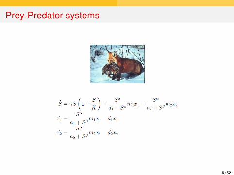
Prey-Predator systems

6/52


Dengue disease (Aedes Aegypti)

7/52


Sustainable development

8/52


Dynamical SystemsIntroduction & Bifurcations

Gerard Olivar

ABC Dynamics - PCI

http://www.manizales.unal.edu.co/gta/abcdynamicshttp://www.manizales.unal.edu.co/gta/PCI

CeiBA Complejidad

Universidad Nacional de Colombia, Sede Manizales

Mathematics of Bio-Economics at IHPJanuary 2013

9/52


Contents

Today: very basicsTomorrow: bifurcations

10/52


Introductory motivation

Outline for today

1 Introductory motivation

2 Basics

3 Nonlinear tools

4 Poincaré maps

5 Examples

11/52



A word about models

How close can we get?

12/52



Dynamical systems: ODEs

As far as this first part of the tutorial, we will only consider sytems ofOrdinary Differential Equations (ODEs)

˙X (t) = F (t ,X (t))

where X is the state vector and F is smooth (say differentiable)NOT F non-smooth (piecewise-smooth)NOT PDEsNOT maps (discrete-time systems), since they will be studied indetail next weekNOT adding stochasticity (stochastic ODEs or PDEs)NOT dynamics on networks (graphs)

although all these other cases appear quite usually in practice

13/52



Dynamical systems: F non-smooth

They usually appear in some control systems where the control is alsonon-smooth (bang-bang, for example)

Depending on the non-smoothness degree, they can be classified intoImpact systems (heaviest non-smoothness, like rigid walls)Filippov systems (sliding systems from control)Piecewise-continuous systems (vector field is continuous at theborder)

14/52



Dynamical systems: PDEs I

Partial differential equations (PDEs)when spatial dimension matters

15/52



Dynamical systems: PDEs II

Wave equation (x = x(t , l1(t), l2(t)))

∂2x∂t2 = c2(

∂2x∂l12 +

∂2x∂l22 )

http://en.wikipedia.org/wiki/Wave_equation

Heat equation (x = x(t , l1(t), l2(t)))

∂x∂t

= b2(∂2x∂l12 +

∂2x∂l22 )

http://en.wikipedia.org/wiki/Heat_equation

16/52

http://en.wikipedia.org/wiki/Wave_equation

http://en.wikipedia.org/wiki/Heat_equation



Dynamical systems: Maps

The discrete TRAP-TRICK

Maps are discrete-time systems. My view is:

We would be really interested in continuous-time systems but theyare more difficult to study and simulate than discrete-time systemsAlso, in practice, is almost impossible to obtain continuous-timeDATAAnd, even if we had the DATA, probably we could not process itadequately

Thus, we are happy enough with a discretization in time of a reallycontinuous-time system

17/52



Dynamical systems: Stochastics and Networks

Adding stochasticity poses a quite difficult problem (at least for me!).Something will be seen in the last part of this trimester.

On networks, the geometry of the state space becomes important(usually is no more isotropic nor homogeneous).

Check http://acn2013.dei.polimi.it

(Milano, 20-22 February 2013)

18/52

http://acn2013.dei.polimi.it



Dynamical systems: ODEs

Thus we will study˙X (t) = F (t ,X (t))

whereX (t) = (x1(t), x2(t), . . . , xn(t))

is the state vector (for short, we will write X or (x1, x2, . . . , xn)), whichlives in Rn,

X = (x1, x2, . . . , xn)

are the time-derivatives of the state and F (so-called vector field) issmooth (say C1)

19/52



From control systems to dynamical systems

Usually, control theorists use the state-space framework

X = F (X ,u)Y = H(X )

(1)

where Y stands for the observable variables and u(Y ) is the controlaction.

This is the so-called control problem, since u(Y ) is still not defined.

But if u(Y ) is already defined, then we have

X = F (X ,u) = F (X ,u(Y )) = F (X ,u(H(x))) = G(x)

and we recover just a dynamical system.

20/52



From optimal control systems to dynamical systems

Finally, in this trimester we want to deal with

Dynamics - Constraints - Optimal Control

Thus...

21/52



Our framework is...

Dynamical systemX = F (t ,X ,u)

ConstraintsX ∈ A u ∈ B

Control optimization criteria

Max L(t ,X ,u) Min L(t ,X ,u)

22/52



Back again to dynamical systems

Once we haveu∗ = u∗(t ,X )

which optimizes L, then solve

X = F (t ,X ,u∗(t ,X )) = G(t ,X )

which is just a dynamical system again

(taking the constraints into account)

23/52


Basics

Outline for today


2 Basics

3 Nonlinear tools

4 Poincaré maps

5 Examples

24/52


Basics

Systems of ODEs

˙X (t) = F (t ,X (t),p)

whereX (t) = (x1(t), x2(t), . . . , xn(t))

is the state vector (for short, we will write X or (x1, x2, . . . , xn)), whichlives in Rn,

X = (x1, x2, . . . , xn)

are the time-derivatives of the state,

F = (F1(x1, x2, . . . , xn),F2(x1, x2, . . . , xn), . . . ,Fn(x1, x2, . . . , xn))

is the smooth vector field (say C1), and

p = (p1,p2, . . . ,pm) ∈ Rm

is the parameters (parameters are unknown constants) vector.25/52


Basics

Study cases

It may be that:F does not depend explicitly on t (autonomous system)F depends T -periodically on t (periodically-forced system)F depends non-periodically on t (non-autonomous system)

Also, it may be thatF is linearF is nonlinear

(comment on linear is to systems as dogs is to animals)

26/52


Basics

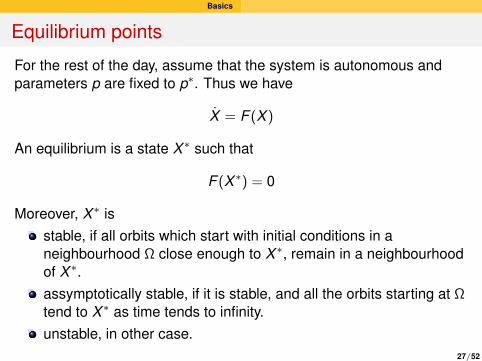
Equilibrium points

For the rest of the day, assume that the system is autonomous andparameters p are fixed to p∗. Thus we have

X = F (X )

An equilibrium is a state X ∗ such that

F (X ∗) = 0

Moreover, X ∗ isstable, if all orbits which start with initial conditions in aneighbourhood Ω close enough to X ∗, remain in a neighbourhoodof X ∗.assymptotically stable, if it is stable, and all the orbits starting at Ωtend to X ∗ as time tends to infinity.unstable, in other case.

27/52


Basics

Linear systems I

Assume we have a linear system

X = F (X ) = AX + b

If det(A) 6= 0 then the unique equilibrium point is X ∗ = −A−1bIf det(A) = 0 then there is an infinite number of non-isolatedequilibrium points (a linear manifold: a line, a plane,...)

28/52


Basics

Linear systems II

Assume we have a linear system

X = F (X ) = AX + b

with equilibrium point X ∗ = −A−1b.If all eigenvalues of A have strictly negative real part then X ∗ isassymptotically stableIf there is an eigenvalue of A with strictly positive real part then X ∗

is unstableIf there are no eigenvalues of A with strictly positive real part, andall eigenvalues with zero real part (thus they are non-zero pureimaginary eigenvalues) have multiplicity one, then X ∗ is stable(but not assymptotically). In this case, the equilibrium point iscalled a center, and it is surrounded by an infinite family ofisochronic periodic orbits.

(other cases are more technical)29/52


Basics

Different configurations in the linear case

See blackboard

30/52


Basics

Nonlinear systems I

Assume we have a nonlinear system

X = F (X )

Now, we can have any number of isolated equilibrium points (evennoone). Moreover there are other stationary sets:

Limit cycles (isolated periodic orbits)Quasiperiodic orbits (if dimension of the state space is at least 3)Chaotic orbits (if dimension of the state space is at least 3)

which can be stable or unstable.

31/52


Basics

Nonlinear systems II

Assume we have a nonlinear system

X = F (X )

and an isolated equilibrium point X ∗.

We compute the jacobian at the equilibrium point

A = Jac(F (X ∗)) = DF (X ∗)

If all eigenvalues of A have strictly negative real part then X ∗ isassymptotically stableIf there is an eigenvalue of A with strictly positive real part then X ∗

is unstable(the case with zero real-part eigenvalues is not solved)

32/52


Basics

Stationary states

33/52


Basics

Transient versus Stationary states

The role of stationary states: take into account thatIf the system has a slow time-constant, sometimes the study ofthe stationary behavior is nonsense, and what is really importantare the possible transient states (sustainable development,sludges, bioreactors,...)If the system has a fast time-constant, although the transient maybe important, the study of the satationary state is worthwhile(circuits, power electronics, powers systems, ...)

34/52


Nonlinear tools

Outline for today


2 Basics

3 Nonlinear tools

4 Poincaré maps

5 Examples

35/52


Nonlinear tools

Invariant manifolds (linear case)

In the linear case, we can considern− = number of strictly negative real-part eigenvaluesn+ = number of strictly positive real-part eigenvaluesn0 = number of zero real-part eigenvalues.

Then we can decompose

Rn = Es ⊕ Eu ⊕ E0

whereEs is the linear stable manifold with dimension n−

Eu is the linear unstable manifold with dimension n+ and,E0 is the linear neutral manifold with dimension n0.

They are expanded by the corresponding eigenvalues (or generalizedeigenvalues).

Note that, since they are linear, they can only meet at the equilibriumpoint X ∗

36/52


Nonlinear tools

Invariant manifolds (nonlinear case)

In the nonlinear case, we can do something similar with the JacobianA = DF (X ∗). We also consider

n− = number of strictly negative real-part eigenvaluesn+ = number of strictly positive real-part eigenvaluesn0 = number of zero real-part eigenvalues.

Then we can decompose (at least, locally)

Rn = W s ⊕W u ⊕W 0

whereW s is the stable manifold with dimension n−

W u is the unstable manifold with dimension n+ and,W 0 is the neutral manifold with dimension n0.

37/52


Nonlinear tools

Invariant manifolds (nonlinear case)

They are expanded locally close to the equilibrium point X ∗ also by thecorresponding eigenvalues (or generalized eigenvalues). This meansthat the linear manifolds are tangent to the invariant manifolds at theequilibrium point.

Note that now, since they are nonlinear surfaces, or curves, a priori,they may meet at points other than the equilibrium point X ∗.

But note also that the existence and uniqueness theorem for ODEsavoids this, and then

the invariant manifolds coincide, orwe have another equilibrium point, or in general, anotherstationary set

38/52


Nonlinear tools

Homoclinic and heteroclinic orbits

In the first case we have a so-called homoclinic connection and, in thesecond case we have an heteroclinic connection.

39/52


Nonlinear tools

Basins of attraction

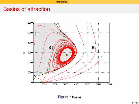
Also, in the nonlinear case, different attractors have their own basin ofattraction, which includes all initial conditions in the state space whoseorbits in positive time reach the attractor.

40/52


Poincaré maps

Outline for today


2 Basics

3 Nonlinear tools

4 Poincaré maps

5 Examples

41/52


Poincaré maps

Poincaré map I

Poincaré maps are often used for discretizing continuous-timesystems, keeping most of the properties of the original one.

ConsiderX = F (t ,X )

and the flow φt corresponding to the orbits of the system.

Consider (locally) a smooth surface Π of dimension n − 1.

Choose an initial condition X0 on Π, and the orbit through X0. If weassume that this orbit hits again Π for first time at time t1 at a pointX1 ∈ Π, we can define this point as the image of X0 through a so-calledPoincaré map P,

P : Π→ Π Π(X0) = X1

42/52


Poincaré maps

Poincaré map I

We can do this for a convenient neighbourhood of X0 as this (local)map is well-defined (some orbits can never go back again to Π)

43/52


Poincaré maps

Poincaré map II

This procedure is specially useful in two situations:When the system is T -periodically forcedClose to a periodic orbit

44/52


Poincaré maps

A T -periodically forced system

In this case, we can rewrite the problem in a cylindrical space Rn × S1,and choose our Poincaré section as the set t = 0 = T. Then thePoincaré map is globally defined (and it is known as a stroboscopicmap).

45/52


Poincaré maps

Close to a periodic orbit

In this case, if L is the periodic orbit, we choose a (local) Poincarésection which is normal to L.

If we choose point q∗ as the intersection of the periodic orbit and thesection, we will have that

P(q∗) = q∗

and thus q∗ is a fixed point of map P.

46/52


Poincaré maps

Close to a periodic orbit

Consider now a neighbourhood of q∗ in Π such that this Poincaré mapis well-defined.

Then all stability properties of L (in the continuous-time system) areequivalent to those of q∗ (as a fixed point of the Poincaré map).The same applies if we consider a quasiperiodic orbit or a chaotic orbit

47/52


Examples

Outline for today


2 Basics

3 Nonlinear tools

4 Poincaré maps

5 Examples

48/52


Examples

Simple model in Sustainable development

Resource dynamics (forest):

dSdt

= ρ

(Sk− 1

)(1− S

K

)S − αβLS

Natural growthResource profit

Population dynamics:

dLdt

= ( γλ (1− β)δ Lδ−1 + φαβS − σ )L

RentsPoverty threshold

49/52


Examples



dSdt

= ρ

(Sk− 1

)(1− S

K

)S − αβLS



dLdt

= ( γλ (1− β)δ Lδ−1 + φαβS − σ )L


49/52


Examples



dSdt

= ρ

(Sk− 1

)(1− S

K

)S − αβLS



dLdt

= ( γλ (1− β)δ Lδ−1 + φαβS − σ )L


49/52


Examples



dSdt

= ρ

(Sk− 1

)(1− S

K

)S − αβLS



dLdt

= ( γλ (1− β)δ Lδ−1 + φαβS − σ )L


49/52


Examples



dSdt

= ρ

(Sk− 1

)(1− S

K

)S − αβLS



dLdt

= ( γλ (1− β)δ Lδ−1 + φαβS − σ )L


49/52


Examples

Phase portrait

Figure : Equilibrium points and nullclines. P4 is assymptotically stable while P6 is unstable andP5 is a saddle

50/52


Examples

Basins of attraction

Figure : Basins

51/52


Examples

End of slides for today...

More examples on the blackboard

52/52

Documents

MABIES Program at IHP - CERMICScermics.enpc.fr/~delara/MABIES/slides_Olivar_dynamics.pdf · escudos/unescudos/ceiba Introductory motivation Dynamical systems: Maps The discrete TRAP-TRICK