MA2213 Lecture 4

Numerical Integration

Introduction

Definition

is the limit of Riemann sums

http://www.slu.edu/classes/maymk/Riemann/Riemann.html

b

axdxI )(f)f(

I(f) is called an integral and the process of calculating it is called integration – it has anenormous range of applications

http://en.wikipedia.org/wiki/Riemann_sum

http://www.intmath.com/Applications-integration/Applications-integrals-intro.php

Method of Exhaustion

was used in ancient times to compute areas and volumes of standard geometric objects

b

axdxI )(f)f(

http://www.ugrad.math.ubc.ca/coursedoc/math101/notes/integration/area.html

Example: area of region between the x-axis, the graph of a function y = f(x), and the vertical lines x = a, and x = b, is given by

http://en.wikipedia.org/wiki/Method_of_exhaustion

Fundamental Theorem of Calculus

(Newton and Leibniz) implies that

where F is any antiderivative of f, this means that

Unfortunately, not all integrands f have ‘closed form’ antiderivatives

],[),(f)( baxxxdx

dF

)exp()(f 2xx

)()()(f)f( aFbFxdxIb

a

Left Riemann Sum

[f(x0) + f(x1) + ... + f(xn-1)] *Delta  x

Right Riemann Sum

[f(x1) + f(x2) + ... + f(xn)] * Delta  x

http://mathews.ecs.fullerton.edu/a2001/Animations/Quadrature/Midpoint/Midpointaa.html

Midpoint Rule Animation

Midpoint Rule

[f(m1) + f(m2) + ... + f(mn)] * Delta  x

http://mathews.ecs.fullerton.edu/a2001/Animations/Quadrature/Midpoint/Midpointaa.html

Animation

2,,

2,

2121

210

1nn

n

xxm

xxm

xxm

Trapezoidal Rule

The trapezoid approximation associated with a

uniform partition a = x0 < x1 < ... < xn = b is given

by .5*[f(x0) + 2f(x1) + ... + 2f(xn-1) + f(xn)]*Delta x

Review Questions

How can the trapezoidal rule be obtained

from the left and right Riemann sums ?

How can the trapezoidal rule be obtained from the midpoint rule ?

How can the trapezoidal rule be obtained by approximating the integral of a f by the integral of an interpolant of f ?

Simpson’s Ruleis obtained by computing the integral

of a quadratic interpolating polynomial

dxabaca

bxcxdxxPI

b

a

b

a)(f

))((

))(()()f( 2

dxbcbab

cxaxc

bcac

bxaxb

a

)(f))((

))(()(f

))((

))((

)(f)(f4)(f6

bcaab

where 2

abc

Simpson’s Rule

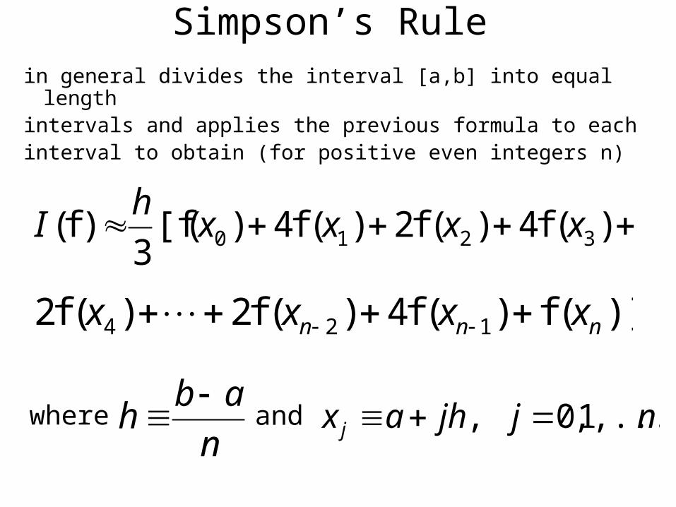
in general divides the interval [a,b] into equal length intervals and applies the previous formula to each interval to obtain (for positive even integers n)

)(f4)(f2)(f4)([f3

)f( 3210 xxxxh

I

where

)](f)(f4)(f2)(f2 124 nnn xxxx

n

abh

and njjhax j ,...,1,0,

Quadrature is based on the exact integration of polynomials

of increasing degree, [a,b] is not subdivided

n

jjjn xwI

1

)(f)f(

Theorem 1 If nodes nxx 1

whenever

nww ,...,1

are given then there exist unique weights

b

an dxxII )(f)f()f(such that

in ],[ ba

f is a polynomial with degree 1-n

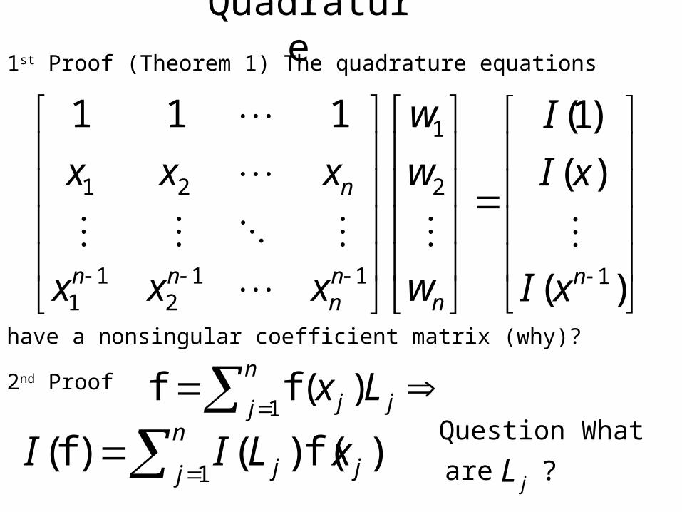
Quadrature 1st Proof (Theorem 1) The quadrature equations

)(

)(

)1(111

1

2

1

112

11

21

nn

nn

nn

n

xI

xI

I

w

w

w

xxx

xxx

have a nonsingular coefficient matrix (why)?

)f()()f(1 j

n

j j xLII

n

j jj Lx1

)(ff2nd Proof

Question What

jLare ?

Gaussian Quadrature is based on strategic choice of nodes

1n

(only a genius could make such a choice) so that

nxx 1

when weights nww ,...,1 are chosen with

)f()f( IIn then also (as if by MAGIC)

for polynomials f with degree

)f()f( IIn for polynomials f with degree 12 n

We seem to get n extra equations for free !

Let us examine cases for n = 1 and for n = 2.

Gaussian Quadrature

Case n = 1 )(f)(f)f( 11

1

1xwdxxI

for polynomials f of as large degree as possible.

21 w

is to hold

For f(x) = 1

Question Why is this quadrature formula

exact for ALL linear polynomials ?

For f(x) = x 01 x

Gaussian Quadrature

Case n = 2 )(f)(f)(f 2211

1

1xwxwdxx

is to hold for the polynomials f(x) = .,,,1 32 xxx

This yields the system of four nonlinear equations

whose solution is

212 ww 22110 xwxw 222

2113

2 xwxw 322

3110 xwxw

121 ww

33

233

1 , xx

Gaussian Quadrature

Example 3504024.211

1

eedxex

Not bad for an estimate based on 2 nodes !

3426961.2)( 3/33/32 eeeI x

00771.0)()( 2 xx eIeI

Question Why is dxxab

dxxb

a

1

1)(f

~

2)(f

where

2

)(f)(f

~ abtabt

and why is

this useful ?

Gaussian Quadrature Case n > 2 Find nn wwxx ,...,,,..., 11

such that

n

j jjn xwIdxx1

1

1)(f)f()(f for

12/)(cf)()()( n2 abhfTfI n

Gauss solved this using orthogonal polynomials.http://en.wikipedia.org/wiki/Gaussian_quadrature

.,...,,,1)(f 122 nxxxx

Error Bounds

Trapezoidal

Simpson 180/)(cf)()()( n)4(4 abhfSfI n

Gauss (f))(2|)()(| 12 nn abfIfI

nabh /)( |)()(f|max min)f( b][a,x)deg( xPxdPd minimax error

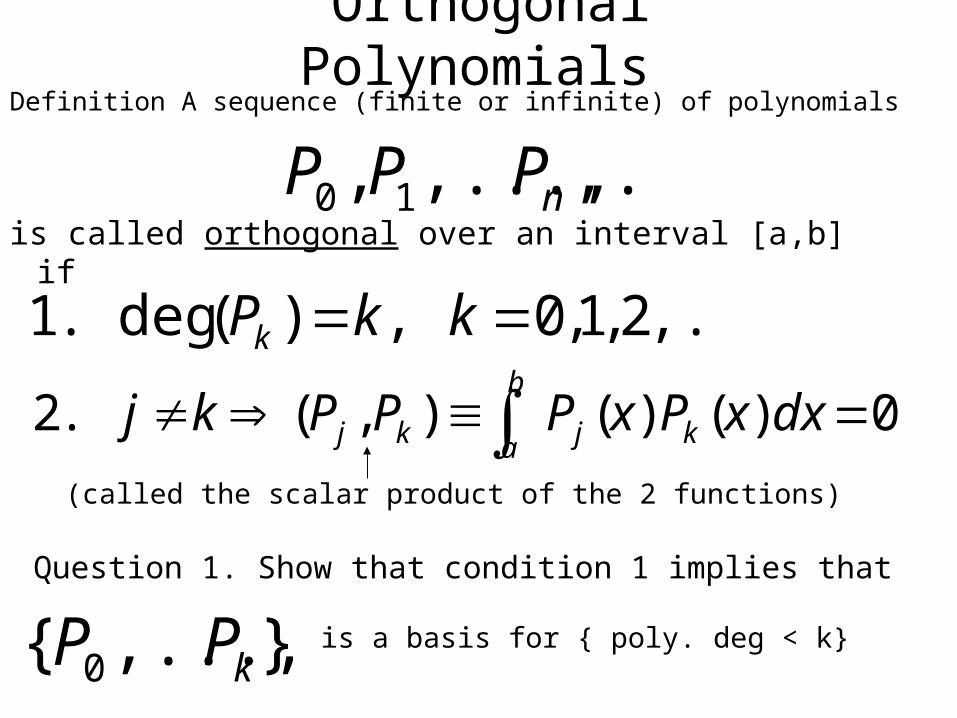
Orthogonal Polynomials Definition A sequence (finite or infinite) of polynomials

is called orthogonal over an interval [a,b] if

Question 1. Show that condition 1 implies that

,...,...,, 10 nPPP

,...2,1,0,)(deg.1 kkPk

0)()(),(.2 dxxPxPPPkj k

b

a jkj

(called the scalar product of the 2 functions)

},...,{ 0 kPP is a basis for { poly. deg < k}

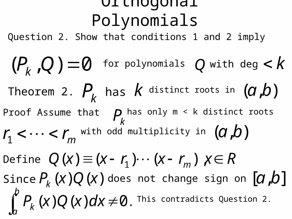
Orthogonal Polynomials

Question 2. Show that conditions 1 and 2 imply

for polynomials kQ

Theorem 2.

0),( QPk with deg

kP has k distinct roots in ),( baProof Assume that has only m < k distinct roots

kPmrr 1

with odd multiplicity in ),( ba

Define RxrxrxxQ m ),()()( 1 Since )()( xQxPk does not change sign on ],[ ba

b

a k dxxQxP .0)()( This contradicts Question 2.

Gaussian Quadrature Theorem 2. If

],[ ba

zeros of

nxx 1

wherenPare chosen to be the

hg nPf

and

are orthogonal

b

aj

n

j jn dxxIxwI )(f)f()f()f(1

by Thm 1 so that whenever f is a poly. deg < n

are chosen

then this same equation holds if f has deg. < 2n

nPPP ,...,, 10

polynomials over nww ,...,1

Proof Divide to obtain where g and hare polynomials with nhng deg,degThen )f()()()()f( IhgPIhIhII knn

Homework Due at End of Lab 2Question 1.

for the function

Compute the least squares approximation

over the interval [-1,1] from the set S

of functions that are continuous on [-1,1] and linear on

[-1,0] and on [0,1]. Express your solution as a linear

combination of the basis functions for S described in the

1st vufoil in Lecture 3. The coefficients of this linear

combination are solutions of a system of 3 linear

equation whose matrix of coefficients is the Gramm

matrix that you computed for Question 4 in the previous

Homework. Write a MATLAB program in an MATLAB

.m-file to solve this linear system of equations.

xe