Embed Size (px)
Citation preview

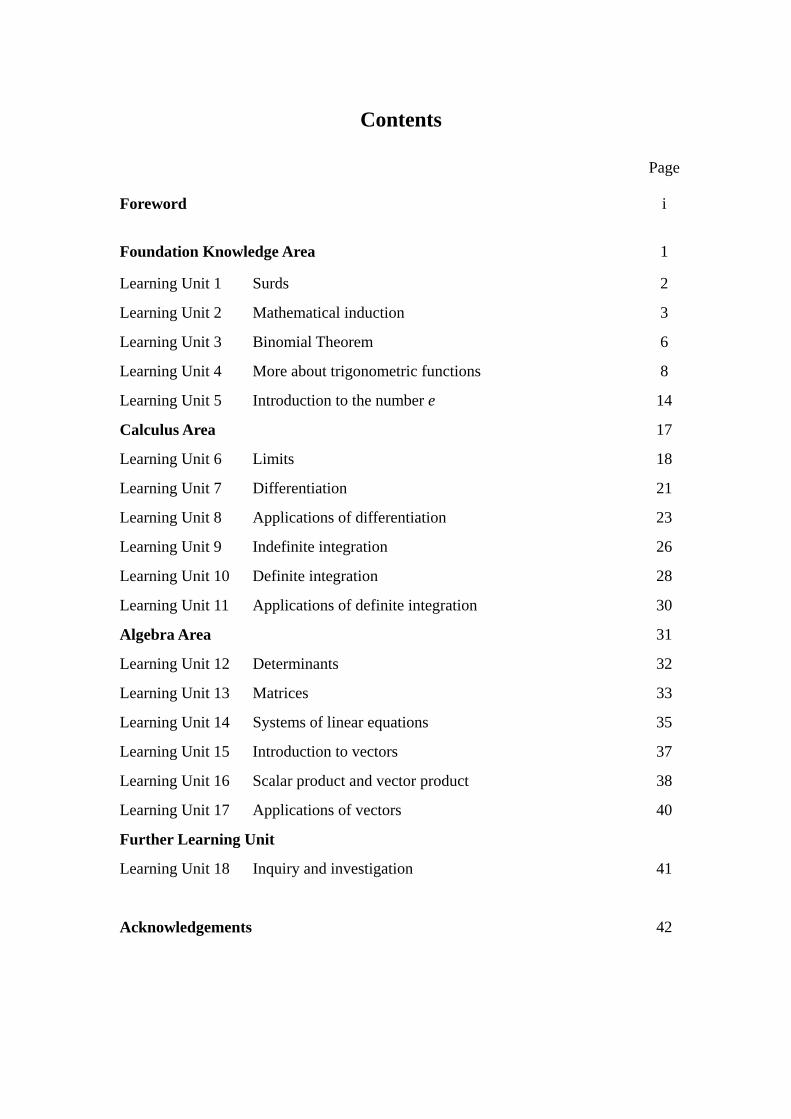
Contents
Page
Foreword i
Foundation Knowledge Area 1
Learning Unit 1 Surds 2
Learning Unit 2 Mathematical induction 3
Learning Unit 3 Binomial Theorem 6
Learning Unit 4 More about trigonometric functions 8
Learning Unit 5 Introduction to the number e 14
Calculus Area 17
Learning Unit 6 Limits 18
Learning Unit 7 Differentiation 21
Learning Unit 8 Applications of differentiation 23
Learning Unit 9 Indefinite integration 26
Learning Unit 10 Definite integration 28
Learning Unit 11 Applications of definite integration 30
Algebra Area 31
Learning Unit 12 Determinants 32
Learning Unit 13 Matrices 33
Learning Unit 14 Systems of linear equations 35
Learning Unit 15 Introduction to vectors 37
Learning Unit 16 Scalar product and vector product 38
Learning Unit 17 Applications of vectors 40
Further Learning Unit
Learning Unit 18 Inquiry and investigation 41
Acknowledgements 42

Copyright: © HKSAR Education Bureau, 2010. Content in this booklet may be used for
non-profit-making educational purposes with proper acknowledgement.
ISBN 978-988-8040-41-4
i
Foreword
The Mathematics Curriculum and Assessment Guide (Secondary 4 – 6) (2007)
(abbreviated as “C&A Guide” in this booklet) has been prepared to support the new
academic structure implemented in September 2009. The Senior Secondary
Mathematics Curriculum consists of a Compulsory Part and an Extended Part. The
Extended Part has two optional modules, namely Module 1 (Calculus and Statistics)
and Module 2 (Algebra and Calculus).
In the C&A Guide, the Learning Objectives of Module 2 are grouped under different
learning units in the form of a table. The notes in the “Remarks” column of the table
in the C&A Guide provide supplementary information about the Learning Objectives.
The explanatory notes in this booklet aim at further explicating:
1. the requirements of the Learning Objectives of Module 2;
2. the strategies suggested for the teaching of Module 2;
3. the connections and structures among different learning units of Module 2; and
4. the curriculum articulation between the Compulsory Part and Module 2.
The explanatory notes in this booklet together with the Remarks column and the
suggested lesson time of each learning unit in the C&A Guide are to indicate the
breadth and depth of treatment required. Teachers are advised to teach the contents
of the Compulsory Part and Module 2 as a connected body of mathematical
knowledge and develop in students the capability to use mathematics to solve
problems, reason and communicate. Furthermore, it should be noted that the
ordering of the Learning Units and Learning Objectives in the C&A Guide does not
represent a prescribed sequence of learning and teaching. Teachers may arrange the
learning content in any logical sequence which takes account of the needs of their
students.
ii
Comments and suggestions on this booklet are most welcomed. They should be sent
to:
Chief Curriculum Development Officer (Mathematics)
Curriculum Development Institute
Education Bureau
4/F, Kowloon Government Offices
405 Nathan Road, Kowloon
Fax: 3426 9265
E-mail: [email protected]
1
Foundation Knowledge Area
The content of Foundation Knowledge Area comprises five Learning Units and is considered
as the pre-requisite knowledge for Calculus Area and Algebra Area of Module 2. These
Learning Units serve to bridge the gap between the Compulsory Part and Module 2.
Therefore, it should be noted that complicated treatment of topics in this Area is not the
objective of the Curriculum.
The Learning Unit “Surds” provides a necessary tool to help students manipulate limits and
derivatives in Calculus Area. The Learning Unit “Binomial Theorem” forms the basis of the
proofs of some rules in the Learning Unit “Differentiation”. Students should be able to prove
propositions by applying mathematical induction. The Learning Unit “More about
trigonometric functions” introduces the radian measure of angles, the six trigonometric
functions and some trigonometric formulae commonly used in the learning of Calculus.
Students should understand the importance of the radian measure in Calculus Area. The
Learning Unit “Introduction to the number e” helps students understand that the natural
logarithm is an important concept in mathematics and is crucial in differentiation as well as
integration in Calculus.
As there is a strong connection between Foundation Knowledge Area and other Areas,
teachers should arrange suitable teaching sequences to suit their students’ needs. For example,
teachers can embed the Learning Unit “Surds” into Learning Unit 6 “Limits” when teaching
differentiation from first principles to form a coherent set of learning contents.
2
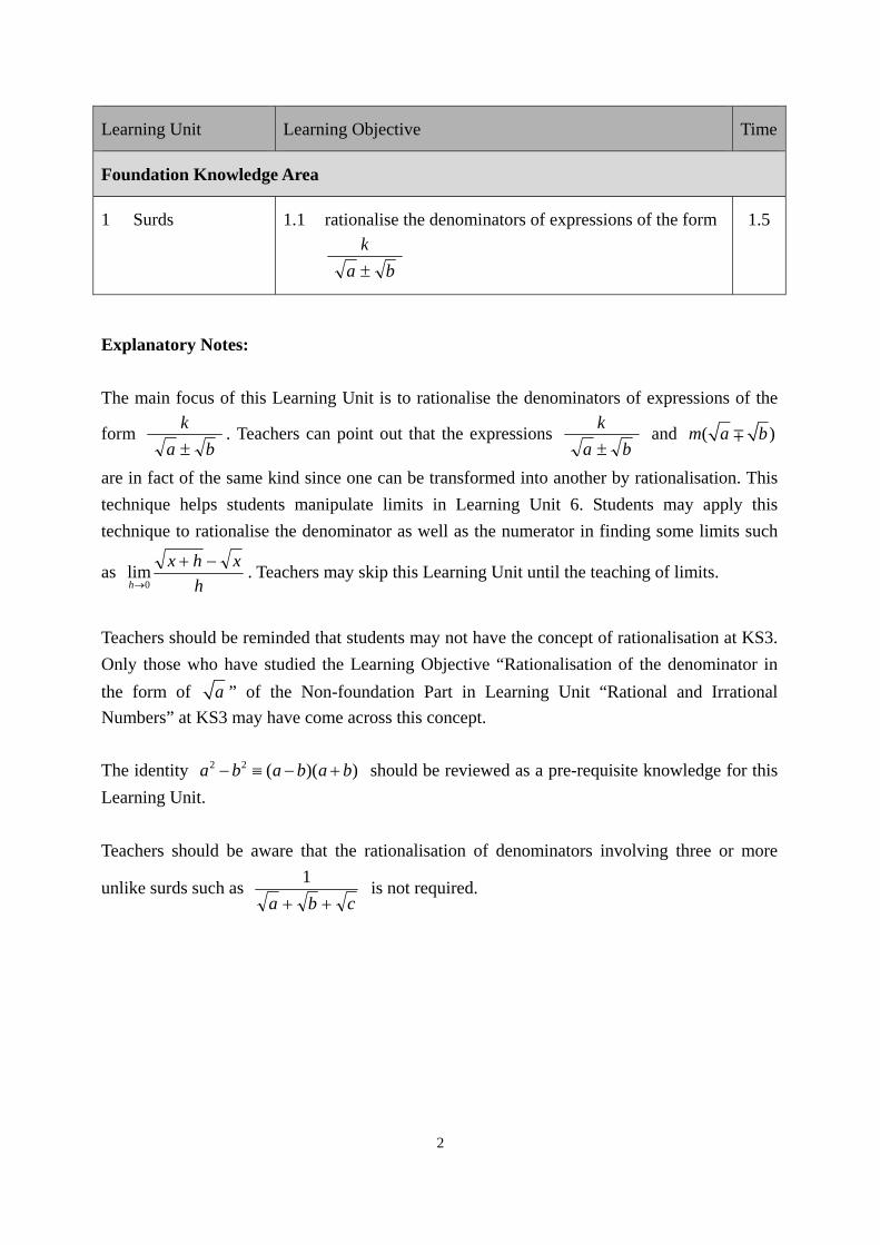
Learning Unit Learning Objective Time
Foundation Knowledge Area
1 Surds 1.1 rationalise the denominators of expressions of the form
ba
k
1.5
Explanatory Notes:
The main focus of this Learning Unit is to rationalise the denominators of expressions of the
form ba
k
. Teachers can point out that the expressions
ba
k
and ( )m a b
are in fact of the same kind since one can be transformed into another by rationalisation. This
technique helps students manipulate limits in Learning Unit 6. Students may apply this
technique to rationalise the denominator as well as the numerator in finding some limits such
as h
xhxh
0
lim . Teachers may skip this Learning Unit until the teaching of limits.
Teachers should be reminded that students may not have the concept of rationalisation at KS3.
Only those who have studied the Learning Objective “Rationalisation of the denominator in
the form of a ” of the Non-foundation Part in Learning Unit “Rational and Irrational
Numbers” at KS3 may have come across this concept.
The identity 2 2 ( )( )a b a b a b should be reviewed as a pre-requisite knowledge for this
Learning Unit.
Teachers should be aware that the rationalisation of denominators involving three or more
unlike surds such as cba
1 is not required.
3
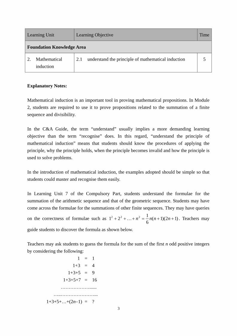
Learning Unit Learning Objective Time
Foundation Knowledge Area
2. Mathematical
induction
2.1 understand the principle of mathematical induction 5
Explanatory Notes:
Mathematical induction is an important tool in proving mathematical propositions. In Module
2, students are required to use it to prove propositions related to the summation of a finite
sequence and divisibility.
In the C&A Guide, the term “understand” usually implies a more demanding learning
objective than the term “recognise” does. In this regard, “understand the principle of
mathematical induction” means that students should know the procedures of applying the
principle, why the principle holds, when the principle becomes invalid and how the principle is
used to solve problems.
In the introduction of mathematical induction, the examples adopted should be simple so that
students could master and recognise them easily.
In Learning Unit 7 of the Compulsory Part, students understand the formulae for the
summation of the arithmetic sequence and that of the geometric sequence. Students may have
come across the formulae for the summations of other finite sequences. They may have queries
on the correctness of formulae such as )12)(1(6
121 222 nnnn . Teachers may
guide students to discover the formula as shown below.
Teachers may ask students to guess the formula for the sum of the first n odd positive integers
by considering the following:
1 = 1
1+3 = 4
1+3+5 = 9
1+3+5+7 = 16
………………......
…..…………………...
1+3+5+…+(2n1) = ?
4
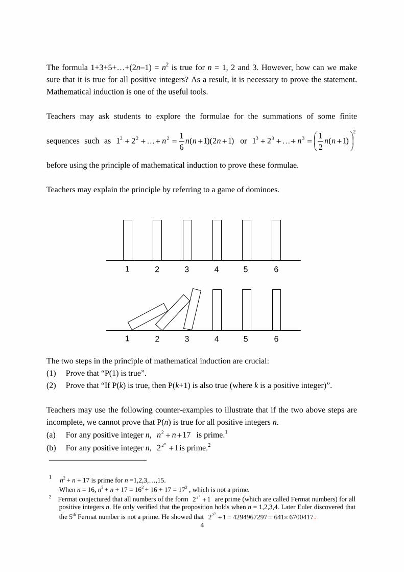
The formula 1+3+5+…+(2n1) = n2 is true for n = 1, 2 and 3. However, how can we make
sure that it is true for all positive integers? As a result, it is necessary to prove the statement.
Mathematical induction is one of the useful tools.
Teachers may ask students to explore the formulae for the summations of some finite
sequences such as )12)(1(6
121 222 nnnn or
2333 )1(
2
121
nnn
before using the principle of mathematical induction to prove these formulae.
Teachers may explain the principle by referring to a game of dominoes.
The two steps in the principle of mathematical induction are crucial:
(1) Prove that “P(1) is true”.
(2) Prove that “If P(k) is true, then P(k+1) is also true (where k is a positive integer)”.
Teachers may use the following counter-examples to illustrate that if the two above steps are
incomplete, we cannot prove that P(n) is true for all positive integers n.
(a) For any positive integer n, 172 nn is prime.1
(b) For any positive integer n, 122 n
is prime.2
1 n2 + n + 17 is prime for n =1,2,3,…,15.
When n = 16, n2 + n + 17 = 162 + 16 + 17 = 172 , which is not a prime. 2 Fermat conjectured that all numbers of the form 122
n
are prime (which are called Fermat numbers) for all positive integers n. He only verified that the proposition holds when n = 1,2,3,4. Later Euler discovered that
the 5th Fermat number is not a prime. He showed that 670041764142949672971252 .
1 2 3 4 5 6
1 2 3 4 5 6

5
(c) For any positive integer n, 22
)1(321
nnn .
(a) and (b) are examples of incomplete induction, in which “P(n) is true” for a finite number of
cases. In the process of proving the statement, step 2 is incomplete. As a result, the statement
“ P(n) is true for all positive integers n” cannot be proved.
Example (c) shows that although we can prove that the statement is true for step 2, P(n) is not
true because P(1) is false.
Teachers could use more examples to demonstrate how to use the principle of mathematical
induction. For examples:
Prove that, for any positive integer n,
(a) )2)(1(6
112)1()2(3)1(21 nnnnnnnn .
(b) 123 n is divisible by 11.
(c) 137 nn is divisible by 9.
(d) 1212 nn ba is divisible by a+b.
Teachers should remind students to pay attention to the proper use of the following terms in
drawing conclusions: numbers, integers, positive numbers and positive integers.
Students should also learn some common variations of the principle. They should be able to
prove propositions like “ nn ba is divisible by ba for all positive even integers n” by
modifying the 2 steps in using the principle of mathematical induction. However, more
complicated variations of the principle of mathematical induction such as the examples below
are not required:
(1) P(1) is true.
(2) If P(n) is true for 1 n k , then P(k+1) is also true (where k is a positive integer).
or
(1) P(1) and P(2) are true.
(2) If P(k1) and P(k) are true, then P(k+1) is also true.
Proving propositions involving inequalities is not required.
Teachers could apply mathematical induction to demonstrate to students the proof of the
binomial theorem in the next Learning Unit.

6
Learning Unit Learning Objective Time
Foundation Knowledge Area
3. Binomial
Theorem
3.1 expand binomials with positive integral indices using
the Binomial Theorem
3
Explanatory Notes:
Students should understand how to prove the Binomial Theorem by the principle of
mathematical induction.
The definition of nrC has been discussed in Learning Unit “Permutation and combination” of
the Compulsory Part. Thus, a combinatorial approach can be used to prove the Binomial
Theorem. The coefficient of the term a3b2 in the expansion of the expression (a+b)5 can be
considered as the number of combinations of choosing two b’s in the expansion of
(a+b)(a+b)(a+b)(a+b)(a+b). It is not difficult for students to understand that 52C is the
coefficient of a3b2 in the expansion of (a+b)5.
In the introduction, students could be asked to find the coefficient of each term in the
expansion (a + b)n by a combinatorial approach and compare the numerical values with those
in Pascal’s triangle3 on the left.
3 The arrangement of the binomial coefficients in a triangle is named after Blaise Pascal as he included this
triangle with many of its application in his treatise, Traité du triangle arithmétique (1654). In fact, in the 13th
century, Chinese mathematician Yang Hui (楊輝) presented the triangle in his book 《詳解九章算法》(1261)
and pointed out that Jia Xian (賈憲) had used the triangle to solve problems. Thus, the triangle is also named
Yang Hui’s Triangle (楊輝三角) or Jia Xian’s Triangle (賈憲三角).

7
1
1 1
1
3 1
1
1 3
2
6 4 1 4 1
C 00
C 10
C 31C 3
0
C 2 2 C 21C 2
0
C 11
C 32 C 3 3
C 41C 4
0 C 42 C 4 3 C 4 4
In general, (a + b)n
= C n 0 a
n+ C n 1 a
n–1b + C
n 2 an–2
b2+...+ C
n n–1abn–1
+ C n n b
n =
r=0
n
C n r a
n–rb
r.
To represent the presentation of the binomial expansion in a more concise form, it is natural
and necessary to introduce the summation notation ( ) to students. It should be aware that
tedious calculations involving the summation notation is not required.
As the Binomial Theorem is a learning unit in the Foundation Knowledge Area, problems and
examples involved should be simple and straightforward. In this connection, the following
contents are not required:
expansion of trinomials
the greatest coefficient, the greatest term and the properties of binomial coefficients
applications to numerical approximation
The Binomial Theorem can also be used to prove 1)( nn nxxdx
d(where n is a positive
integer) from first principles.

8
Learning Unit Learning Objective Time
Foundation Knowledge Area
4. More about
trigonometric
functions
4.1 understand the concept of radian measure
4.2 find arc lengths and areas of sectors through radian
measure
4.3 understand the functions cosecant, secant and cotangent
and their graphs
4.4 understand the identities
1 + tan2 = sec2 and 1 + cot2 = cosec2
4.5 understand compound angle formulae and double angle
formulae for the functions sine, cosine and tangent, and
product-to-sum and sum-to-product formulae for the
functions sine and cosine
11
Explanatory Notes:
At KS3, students learnt how to measure angles in degrees and find the arc lengths and areas of
sectors by using proportions. In Module 2, students will learn how to measure angles in
radians and to find the arc lengths and areas of sectors by formulae in radians. The formula
0
sinlim
= 1 in the Remarks column of Learning Objective 6.2 only holds when is in
radians. Thus, in dealing with problems in Calculus, all angles related to trigonometric
functions are in radians.
In Learning Objective 13.1 of the Compulsory Part, students have learnt the trigonometric
functions sine, cosine and tangent, and their graphs and properties (including maximum and
minimum values and periodicity). Students are expected to learn the other three trigonometric
functions (cosecant, secant and cotangent), their graphs and properties in this Module. As
students have to sketch and compare graphs of various types of functions including
trigonometric functions in Learning Objective 9.1 of the Compulsory Part, it is natural to
expect students to be able to sketch the graphs and properties of the other three trigonometric
functions from those of the three they learnt. In this connection, teachers may start to guide
students to sketch the graph of )(
1
xfy from the given graph of )(xfy and then

9
explore the graph of y = cosec from that of siny . Students should be able to explore
and understand the domains, maximum or minimum values, symmetry and periodicity of the
function y = cosec . They can further sketch the graphs of secant and cotangent and discover
their properties.
Students at KS3 should have learnt the identity sin2 + cos2 = 1. They should be able to
derive from it the other two identities 1 + tan2 = sec2 and 1 + cot2 = cosec2 . Students
are also expected to simplify trigonometric expressions by using these identities.
Teachers may use the following figure to illustrate the six trigonometric ratios and their
relations and guide students to discover the above identities. The circle in the figure below is a
unit circle.
By rotating the shaded triangle of the above figure to a new position, the following figure is
obtained.
1
cos
cot
sin
tan
cosec
sec cosec
cot cos
1
cos
cot
sin
tan cosec
sec

10
By adding two dotted lines in the figure, we have:
The trigonometric identities sin2 + cos2 = 1, 1 + tan2 = sec2 and 1 + cot2 = cosec2
can be observed from the figure above. It is noted that all angles in the proof shown in the
above figures are acute.
Students will find the list of formulae in the Remarks column of Learning Unit 4 on pp.68-69
of the C&A Guide very useful in solving problems related to trigonometric functions.
Teaches may use diagrams to derive the compound angle formulae
sin(A B) = sin A cos B cos A sin B and cos(A B) = cos A cos B sin A sin B.
Other formulae could then be derived from these four basic formulae.
Different related proofs of the above four basic formulae could be found in reference
books/textbooks. Some non-traditional proofs are included here for teachers’ reference. It is
reminded that, in general, there are restrictions on the sizes of angles in the proofs which
depend on diagrams.
sec
1
cot
sin
tan
cosec
cos
11
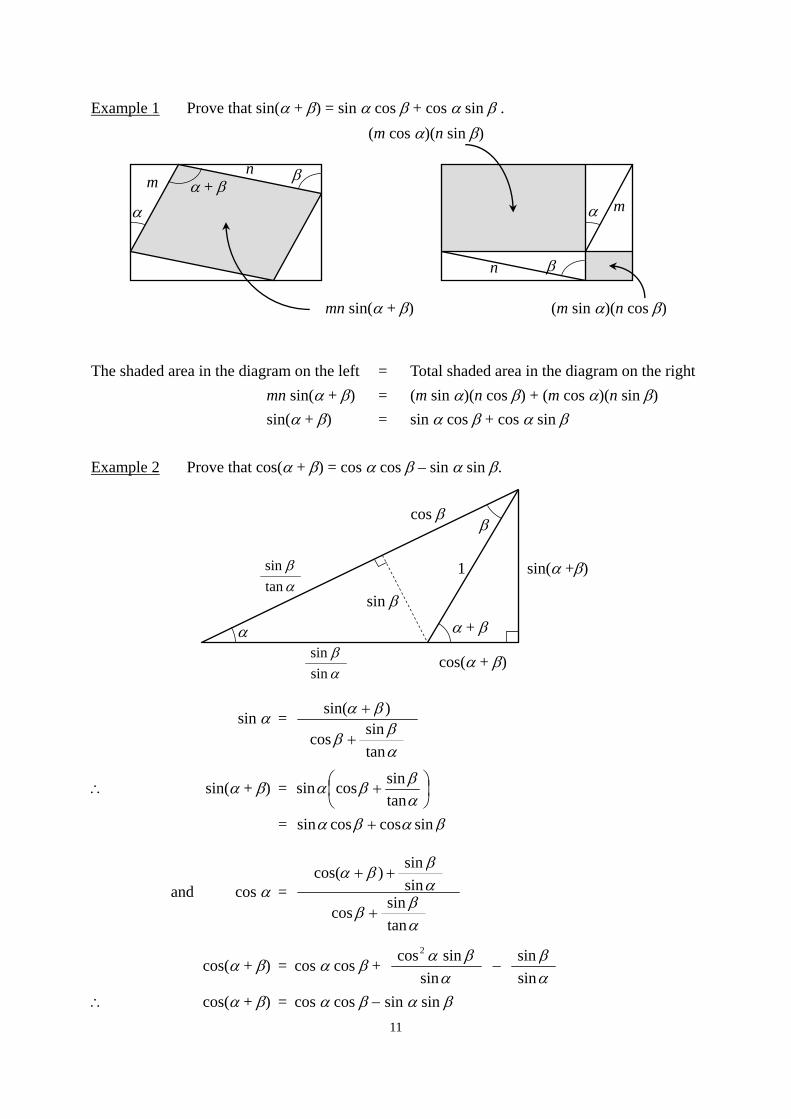
Example 1 Prove that sin( + ) = sin cos + cos sin .
The shaded area in the diagram on the left = Total shaded area in the diagram on the right
mn sin( + ) = (m sin )(n cos ) + (m cos )(n sin )
sin( + ) = sin cos + cos sin
Example 2 Prove that cos( + ) = cos cos – sin sin .
sin =
tan
sincos
)sin(
sin( + ) =
tan
sincossin
= sincoscossin
and cos =
tan
sincos
sin
sin)cos(
cos( + ) = cos cos +
sin
sincos2
sin
sin
cos( + ) = cos cos sin sin
(m cos )(n sin )
(m sin )(n cos )
+ m
n
n
m
mn sin( + )
+
cos
sin
cos( + )
sin( +)
tan
sin
sin
sin
1
12
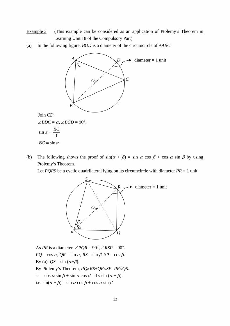
Example 3 (This example can be considered as an application of Ptolemy’s Theorem in
Learning Unit 18 of the Compulsory Part)
(a) In the following figure, BOD is a diameter of the circumcircle of ABC.
Join CD.
BDC = , BCD = 90.
1
sinBC
sinBC
(b) The following shows the proof of sin( + ) = sin cos + cos sin by using
Ptolemy’s Theorem.
Let PQRS be a cyclic quadrilateral lying on its circumcircle with diameter PR = 1 unit.
As PR is a diameter, PQR = 90, RSP = 90. PQ = cos , QR = sin , RS = sin , SP = cos .
By (a), QS = sin (+).
By Ptolemy’s Theorem, PQRS+QRSP=PRQS.
cos sin + sin cos = 1 sin ( + ).
i.e. sin( + ) = sin cos + cos sin .
A
B
C
diameter = 1 unit
O
D
S
P Q
diameter = 1 unit
O
R
13
2 1sin 1 cos 2
2A A and 2 1
cos 1 cos 22
A A can be derived from the double angle
formulae. These formulae, together with the product-to-sum and sum-to-product formulae, are
important tools in finding integrals. Half angle formulae, triple angle formulae, t-formulae and
the “subsidiary angle form” are not required in teaching this Learning Unit.
In Learning Objective 13.2 of the Compulsory Part, students should be able to solve simple
trigonometric equations with solutions in the interval from 0 to 360. In this regard, students
should be able to solve trigonometric equations with solutions from 0 to 2 only. The
discussion of this section can be applied to solve optimisation problems in Learning Objective
8.4.

14
Learning Unit Learning Objective Time
Foundation Knowledge Area
5. Introduction to the
number e
5.1 recognise the definitions and notations of the number e
and the natural logarithm
1.5
Explanatory Notes:
Learning Units 3 and 5 of the Compulsory Part belong to the Non-foundation Topics, in which
the exponential and logarithmic functions and their graphs have been discussed. The number e
and the natural logarithm are introduced as important concepts in mathematics. They are
crucial in the learning of Calculus. Students will learn the exponential function xe in this
Learning Unit.
In general, there are two common approaches to introduce e:
(1) n
n ne )
11(lim
(2) !3!2
132 xx
xe x
Module 2 (Algebra and Calculus) emphasises the first approach.
The following calculation of the amount at compound interest can be employed as an example
to illustrate e.
An amount of money is deposited in a bank for one year at an interest rate of 1% p.a. What
will be the amount if it is compounded
(i) quarterly?
(ii) monthly?
(iii) daily?
(iv) hourly?
(v) every second?
The discussion of the limit n
n n)
11(lim
can be introduced from these questions.

15
The Monotone Convergence Theorem4 is required to prove the existence of e. Nevertheless, it
is not included in this Curriculum. Therefore, students are not required to prove the existence
of the limit.
Furthermore, it can be showed to students that lim(1 )n x
n
xe
n .
The second approach involves the expansion of the binomial expression n
n
x)1( and is
adopted in Module 1 (Calculus and Statistics).
0
0 1 2 30 1 2 3
2 3
2 3
(1 ) ( )
( ) ( ) ( ) ( ) ... ( ) ... ( )
( 1) ( 1)( 2) ( 1)( 2)...( 1)1 ... ...
1! 2! 3! !
nn n r
rr
n n n n n r n nr n
r
r
x xC
n n
x x x x x xC C C C C C
n n n n n n
n x n n x n n n x n n n n r x
n n n r n
2 3
( 1)...( 1)
!
1 1 2 1 2 11 (1 ) (1 )(1 ) ... (1 )(1 ) (1 )
2! 3! !
1 2 1(1 )(1 ) (1 )
!
n
n
r
n
n n n n x
n n
x x r xx
n n n n n n r
n x
n n n n
!3!21
!)
11)...(
21)(
11(...
!)
11)...(
21)(
11(...
!3)
21)(
11(
!2)
11(1lim
)1(lim
32
32
xxx
n
x
n
n
nn
r
x
n
r
nn
x
nn
x
nx
n
xe
n
r
n
n
n
x
By putting x = 1, we have
!8
1
!7
1
!6
1
!5
1
!4
1
!3
1
!2
1
!1
11e
and, by using a calculator, it can be shown that the value of e converges approximately to
2.71828.
4 The Monotone Convergence Theorem states that every monotonic increasing sequence which is bounded
above converges and every monotonic decreasing sequence which is bounded below converges.
16
Teachers should remind students that the natural logarithmic function possesses all properties
of the common logarithm function. Teachers need not treat the natural logarithmic function as
a new category of functions. The formula for change of base, especially in finding derivatives
of logarithms of different bases, is very important in the following learning units. Therefore,
the content of Learning Objective 3.3 of the Compulsory Part involving the formula for change
of base should be reviewed.
This Learning Unit can also be introduced before teaching Learning Objective 6.1.

17
Calculus Area
The Calculus Area consists of “Limits and Differentiation” and “Integration”.
Students need to master the concepts of functions, their graphs and properties to study
“Limits and Differentiation”. Besides, the techniques of manipulating surds help them tackle
many problems of limits. Students can apply the Binomial Theorem to prove the formula
1)( nn nxxdx
d, where n is a positive integer.
Teachers can further lead students to appreciate the beauty of mathematics such as the
irrational number e, the function ex and its derivative. Students can also discover the
importance of differentiation to solve problems related to rate of change, maximum and
minimum.
The indefinite integral and differentiation are related as reverse processes to each other. The
Fundamental Theorem of Calculus links up the two apparently different concepts. At this
stage, one of the applications of the definite integral is to find the area of a plane figure and
the volume of a solid of revolution. Students can also appreciate how to apply the definite
integral to calculate the areas of non-rectilinear figures such as areas of circles, etc.

18
Learning Unit Learning Objective Time
Calculus Area
Limits and Differentiation
6. Limits 6.1 understand the intuitive concept of the limit of a
function
6.2 find the limit of a function
5
Explanatory Notes:
“Limit” is the most fundamental concept in Calculus. After studying Learning Units 2 and 9 of
the Compulsory Part, students should have a comprehensive understanding of the concepts of
various functions and their graphs. However, the functions they met are, in general,
continuous. In this Learning Unit, students will encounter a variety of discontinuous functions
and discuss some properties of discontinuous functions. The introduction of this topic can be
started from the graphs of continuous functions as well as from those of discontinuous
functions. The intuitive concept of the limit of a function can also be developed. Graphing
software is very useful in the exploration of the graphs of functions. It should be noted that the
rigorous definition of the limit of a function is not required in this Curriculum.
To illustrate the continuity of functions, the absolute value function x , the signum function
sgn(x), the ceiling function x and the floor function x may be introduced to students. It
should be noted that these functions are examples only. The formal definition of continuity is
not required. Manipulations of the absolute value function, the differentiation and integration
of the absolute value function are not required.
The following examples can be employed to discuss with students whether certain limits exist
by considering the graphs of the corresponding functions.
(a) Let xxf )( , find )(lim0
xfx
.
(b) Let
1,1
1,)(
2
xx
xxxf , find )(lim
1xf
x.
19
(c) Let 1
2)(
xxf , find )(lim
1xf
x.
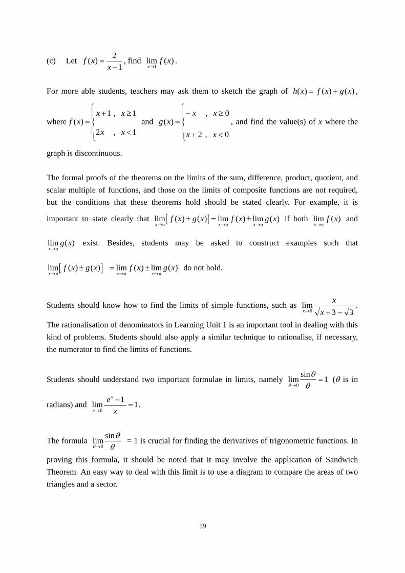
For more able students, teachers may ask them to sketch the graph of )()()( xgxfxh ,
where
1,2
1,1)(
xx
xxxf and
0,2
0,)(
xx
xxxg , and find the value(s) of x where the
graph is discontinuous.
The formal proofs of the theorems on the limits of the sum, difference, product, quotient, and
scalar multiple of functions, and those on the limits of composite functions are not required,
but the conditions that these theorems hold should be stated clearly. For example, it is
important to state clearly that lim ( ) ( ) lim ( ) lim ( )x a x a x a
f x g x f x g x
if both lim ( )x a
f x
and
lim ( )x a
g x
exist. Besides, students may be asked to construct examples such that
lim ( ) ( )x a
f x g x
lim ( ) lim ( )x a x a
f x g x
do not hold.
Students should know how to find the limits of simple functions, such as 33
lim0 x
xx
.
The rationalisation of denominators in Learning Unit 1 is an important tool in dealing with this
kind of problems. Students should also apply a similar technique to rationalise, if necessary,
the numerator to find the limits of functions.
Students should understand two important formulae in limits, namely 0
sinlim 1
( is in
radians) and 0
1lim 1
x
x
e
x
.
The formula
sinlim
0 = 1 is crucial for finding the derivatives of trigonometric functions. In
proving this formula, it should be noted that it may involve the application of Sandwich
Theorem. An easy way to deal with this limit is to use a diagram to compare the areas of two
triangles and a sector.

20
To introduce the formula 0
1lim 1
x
x
e
x
, the substitution x = ln(1+h) and the definition of
xe can be used to prove the formula. This formula can be used to find the derivative of ex.
Students may be asked to guess the value of the limit x
ex 1 as x approaches 0 by referring
to the formula !3!2
132 xx
xex .
Finding the limit of a rational function at infinity is required except those involving the
application of the technique of partial fractions.

21
Learning Unit Learning Objective Time
Calculus Area
Limits and Differentiation
7. Differentiation 7.1 understand the concept of the derivative of a function
7.2 understand the addition rule, product rule, quotient rule
and chain rule of differentiation
7.3 find the derivatives of functions involving algebraic
functions, trigonometric functions, exponential
functions and logarithmic functions
7.4 find derivatives by implicit differentiation
7.5 find the second derivative of an explicit function
14
Explanatory Notes:
Students should be able to find, from first principles, the derivatives of elementary functions,
such as constant functions, xn (n is a positive integer), x , sin x, cos x, ex and ln x. They are
expected to apply the technique of rationalisation to find the derivatives of functions, such as
1
1
x, from first principles. The Binomial Theorem is required to support the proof of
1)( nn nxxdx
d, where n is a positive integer, from first principles. Teachers may also prove
this formula by mathematical induction.
Students should be familiar with notations such as y', f '(x) and dx
dyfor derivatives. Tests of
differentiability of functions are not required.
Students should be able to apply the addition rule, product rule, quotient rule and chain rule to
find the derivatives of functions. It should be noted that students do not have to learn the
concept of composite function in the Compulsory Part. Presentations like
xxdx
xd
xd
xdx
dx
dcossin2
)(sin
)(sin
)(sin)(sin
22 would be helpful for students to understand the
chain rule.

22
To find the derivatives of logarithmic functions with base not equal to e, it is needed to use the
“change of base” formula learnt in Learning Objective 3.3 (Non-foundation Topics) of the
Compulsory Part.
For example, xy 2log
)(log2 xdx
d
dx
dy
2ln
1)(ln
2ln
1
2ln
ln
xx
dx
dx
dx
d
.
It should be explained to students that implicit differentiation is a useful tool in finding
derivatives without having to express the dependent variable in terms of the independent
variable. Equations like 33 33 yxyx and 2yyx are examples for illustrating the use
of implicit differentiation to find dx
dy. It is not easy and sometimes not possible to express y in
terms of x for some equations. For the purpose of differentiating, it is not necessary to express
y in terms of x.
Equations such as 2 2 6( 2)(3 2) (4 5)y x x x and 4
2 1
2 1
xy
x
can be used as examples to
demonstrate the technique of logarithmic differentiation.
Finding the second derivatives of implicit functions has no wide applications in this Module.
Students are expected to find the second derivatives of explicit functions only. The second
derivatives are useful in finding the extrema of functions in Learning Objective 8.2. Notations
such as y", f "(x) and 2
2
dx
yd should be introduced. Third and higher order derivatives are not
required.

23
Learning Unit Learning Objective Time
Calculus Area
Limits and Differentiation
8. Applications of
differentiation
8.1 find the equations of tangents and normals to a curve
8.2 find maxima and minima
8.3 sketch curves of polynomial functions and rational
functions
8.4 solve the problems relating to rate of change, maximum
and minimum
14
Explanatory Notes:
The contents of Learning Objectives 2.3 and 2.4 (Non-foundation Topics) of the Compulsory
Part include the use of the graphical method or the algebraic method to find the
maximum/minimum value of a quadratic function. In Module 2 (Algebra and Calculus),
differentiation is not restricted to solve optimisation problems of quadratic functions.
In Learning Objective 8.1, students are required to find not only the equations of tangents and
normals passing through a given point on a given curve, but also the equations of the tangents
passing through an external point. As it involves using the algebraic method to solve
simultaneous equations in two unknowns, one linear and one quadratic, students should have a
more comprehensive understanding of Learning Objective 5.2 (Non-foundation Topics) of the
Compulsory Part.
The first derivative test and the second derivative test may be used to find local extrema (i.e.
maxima and minima) of functions. In addition to the local extrema, the values of the function
at the endpoints of a closed interval should be considered to determine the global extrema.
When 0)( 0 xf , the second derivative test is not applicable to determine the extrema at
0xx . In this case, students have to use the first derivative test.
Students need to be able to use the second derivative to determine the concavity and convexity
of a function and use these properties to find the points of inflexion of functions.
Teachers should note that curve sketching is restricted to polynomial functions and rational

24
functions only. Certain features of a curve can be observed, or easily obtained, from the
equation of the curve, for example,
symmetry of the curve
limitations on the values of x and y
intercepts with the axes
maximum and minimum points
points of inflexion
vertical, horizontal and oblique asymptotes to the curve
It is not necessary to consider all of these features when examining a particular curve. As
different features will be considered in different problems, it is required to demonstrate the
application of each by different examples.
The properties of convexity and concavity and the concepts of increasing and decreasing
functions are useful in curve sketching. The tangent to a curve at a point of inflexion crosses
the curve. It may be horizontal, oblique and even vertical. Discussions on finding the oblique
asymptote should not involve complicated calculations of limits. It is sufficient for students to
deduce the equation of the oblique asymptote to the graph of a rational function by long
division. Therefore, students’ concepts on the division of polynomials learnt in Learning
Objective 4.1 of the Compulsory Part should be consolidated.
Before solving word problems of maxima and minima, students should note the following
points:
(1) Local maximum and minimum values of a continuous function occur alternately.
(2) If a function has only one turning point, it is obvious, from the nature of the problem, to
determine whether it is a maximum or a minimum point.
In solving problems related to extrema, it should pointed out that using derivatives is
sometimes not the only way to find the maximum or minimum values of a function.
Completing the square is a useful algebraic method to find the maximum or minimum values
of quadratic functions. In dealing with word problems, considerations of the physical
situations of the problems sometimes provide excellent clues. The following examples can be
solved by differentiation. However, the solutions from considering their physical situations are
more elegant than those by using the method of Calculus.
25
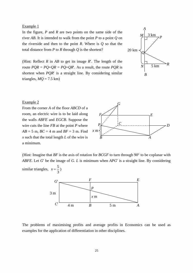
Example 1
In the figure, P and R are two points on the same side of the
river AB. It is intended to walk from the point P to a point Q on
the riverside and then to the point R. Where is Q so that the
total distance from P to R through Q is the shortest?
(Hint: Reflect R in AB to get its image R. The length of the
route PQR = PQ+QR = PQ+QR. As a result, the route PQR is
shortest when PQR is a straight line. By considering similar
triangles, MQ = 7.5 km)
Example 2
From the corner A of the floor ABCD of a
room, an electric wire is to be laid along
the walls ABFE and EGCB. Suppose the
wire cuts the line FB at the point P where
AB = 5 m, BC = 4 m and BF = 3 m. Find
x such that the total length L of the wire is
a minimum.
(Hint: Imagine that BF is the axis of rotation for BCGF to turn through 90 to be coplanar with
ABFE. Let G be the image of G. L is minimum when APG is a straight line. By considering
similar triangles, 3
5x )
The problems of maximising profits and average profits in Economics can be used as
examples for the application of differentiation in other disciplines.
G
F
P
B
C
E
A
Dx m
20 km
3 km
5 km N
Q
M P
R
A
B
G F E
A B C
P
5 m 4 m
3 m x m
26
Learning Unit Learning Objective Time
Calculus Area
Integration
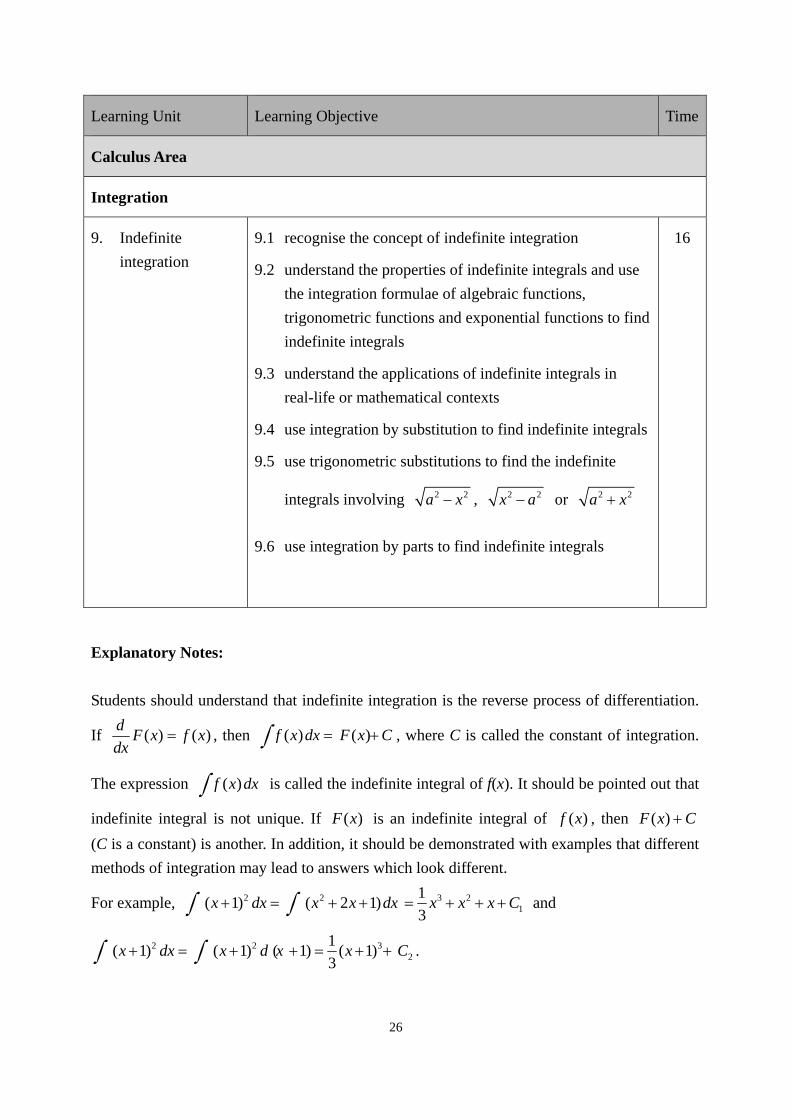
9. Indefinite
integration
9.1 recognise the concept of indefinite integration
9.2 understand the properties of indefinite integrals and use
the integration formulae of algebraic functions,
trigonometric functions and exponential functions to find
indefinite integrals
9.3 understand the applications of indefinite integrals in
real-life or mathematical contexts
9.4 use integration by substitution to find indefinite integrals
9.5 use trigonometric substitutions to find the indefinite
integrals involving 2 2a x , 2 2x a or 2 2a x
9.6 use integration by parts to find indefinite integrals
16
Explanatory Notes:
Students should understand that indefinite integration is the reverse process of differentiation.
If )()( xfxFdx
d , then ( ) ( )f x dx F x C , where C is called the constant of integration.
The expression ( ) f x dx is called the indefinite integral of f(x). It should be pointed out that
indefinite integral is not unique. If )(xF is an indefinite integral of )(xf , then CxF )(
(C is a constant) is another. In addition, it should be demonstrated with examples that different
methods of integration may lead to answers which look different.
For example, 2 2 3 21
1( 1) ( 2 1)
3x dx x x dx x x x C and
2 2 32
1( 1) ( 1) ( 1) ( 1)
3x dx x d x x C .

27
Students may be asked to show that 3
121 CC and note that these two answers only differ
by a constant term.
The formulae in the Remarks column of Learning Objective 9.2 should be understood instead
of rote memorization. In deducing the formula1
lndx x Cx , the absolute value x
should be introduced. Students are not required to learn the indefinite integral ( ) f x dx ,
where )(xf involves absolute values.
Integration by substitutions and integration by parts are useful tools to find indefinite integrals.
In trigonometric substitutions, functions such as sin1 x , cos1 x and tan1x may appear in the
answers. As students do not have the concepts of inverse functions, teachers should discuss
with students the notations of these inverses and introduce their principal values. It should be
noted that integrands containing inverse trigonometric functions are not required.
Problems involving partial fractions are not included in this Module.
It is appropriate that the use of integration by parts is restricted to at most two times in finding
an integral to avoid tedious calculations. Reduction formulae of integration are not included.

28
Learning Unit Learning Objective Time
Calculus Area
Integration
10. Definite
integration
10.1 recognise the concept of definite integration
10.2 understand the properties of definite integrals
10.3 find definite integrals of algebraic functions,
trigonometric functions and exponential functions
10.4 use integration by substitution to find definite integrals
10.5 use integration by parts to find definite integrals
10.6 understand the properties of the definite integrals of
even, odd and periodic functions
11
Explanatory Notes:
The basic definition of the definite integral as the limit of a sum should be introduced to
students. Students may confuse the notation of the definite integral with that of the indefinite
integral. It is expected to introduce to students the Fundamental Theorem of Calculus as a
connection between the two concepts. The proof of the Fundamental Theorem of Calculus is
also required.
Students should understand the concept of dummy variables in definite integrals. All properties
of definite integrals in the Remarks column of Learning Objective 10.2 should be highlighted
to students.
Discussions on properties of the definite integrals for even, odd and periodic functions help
students deepen their understanding on definite integrals.
Students should understand the application of integration by substitution in proving the
properties stated in the Remarks column of Learning Objective 10.6.
Teachers should note that the followings are not required:
the evaluation of the definite integral ( ) b
af x dx , where )(xf involves absolute values
reduction formulae
29
the evaluation of the sum to infinity of a sequence by using a definite integral improper integrals
the inequality ( ) ( ) b b
a af x dx f x dx

30
Learning Unit Learning Objective Time
Calculus Area
Integration
11. Applications of
definite
integration
11.1 understand the application of definite integrals in
finding the area of a plane figure
11.2 understand the application of definite integrals in
finding the volume of a solid of revolution about a
coordinate axis or a line parallel to a coordinate axis
7
Explanatory Notes:
In this Module, the applications of definite integration only confine to the calculations of areas
of plane figures and volumes of solids of revolution. A geometric demonstration on the
relationship between the definition of the definite integral and the area of a plane figure may
be given. Students may be led to appreciate the application of definite integration in providing
a rigorous way to prove the formulae of the area of circle, the volume of right circular cone
and the volume of sphere. The difference between the volumes of solids of revolution about
the coordinate axes or straight lines parallel to them should be discussed.
Both the “disc method” and the “shell method” are included. An intuitive geometric
explanation should be given though a formal proof is not required. In some cases, the “shell
method” is better than the “disc method” in finding the volume of revolution of certain objects.
For example, in finding the revolution of the area bounded by the curve xxy sin and the
lines 0 ,2
y x
about the y-axis, it is easy to use the “shell method”. Teachers may
compare the two methods in finding the volume of the same solid of revolution.
Finding the volume of a hollow solid is required.
31
Algebra Area
The Algebra Area consists of “Matrices and Systems of Linear Equations” and “Vectors”.
In this Area, students encounter a new mathematics structure, “Matrices” , in Algebra. They
will find that the multiplication of matrices is not commutative. This new concept is different
from what they have experienced in the past. They are required to understand the concepts,
operations and properties of matrices, the existence of inverse matrices and the determinants.
Determinants are important tools to investigate the properties of matrices.
At KS3, students solved linear equations in two unknowns by the algebraic method and the
graphical method. Those who studied the enrichment topic “explore simultaneous equations
that are inconsistent or that have no unique solution” at KS3 may have the preliminary
concepts of “consistency” and “inconsistency”. In this Area, students further explore the
conditions of consistency or inconsistency in a system of linear equations. They should be
able to use Cramer’s rule, inverse matrices and Gaussian elimination to solve systems of
linear equations. They should also understand the strengths and weaknesses of each method
and how to choose appropriate methods to solve problems.
In order to extend students’ knowledge in Algebra Area, the concepts, operations and
properties of vectors should be introduced. The scalar product and the vector product are two
useful tools to investigate the geometric properties of vectors including parallelism and
orthogonality. In addition, students can learn to use the vector method to find the volume of a
parallelepiped, the angle between two vectors and the area of a triangle or a parallelogram,
etc.

32
Learning Unit Learning Objective Time
Algebra Area
Matrices and Systems of Linear Equations
12. Determinants 12.1 recognise the concept and properties of determinants of
order 2 and order 3
3
Explanatory Notes:
Determinant is a vital tool in the learning of matrices and systems of linear equations.
Students are expected to learn the basic operations and basic properties of determinants of
order 2 and order 3. The properties are shown in the Remarks column on pp.80-81 of the
C&A Guide.
Students should know that both | A | and det(A) are common notations of the determinant of the
matrix A.
Teachers could introduce one of the uses of determinant as stated below.
In the figure, OAPC is a parallelogram passing through the origin O where
A=(a,b) and C=(c,d).
Area of parallelogram OAPC = a b
c d.
y
x
C(c,d)
A(a,b)
P
O
33
Learning Unit Learning Objective Time
Algebra Area
Matrices and Systems of Linear Equations
13. Matrices 13.1 understand the concept, operations and properties of
matrices
13.2 understand the concept, operations and properties of
inverses of square matrices of order 2 and order 3
9
Explanatory Notes:
The general proof of BAAB in Learning Objective 13.1 is a bit difficult for average
students. In teaching this property, it can be verified by examples without proving. However,
teachers may have more in-depth discussions on this property with students for square
matrices up to order 3 since the proofs are simpler.
Although the identity matrix and zero matrix are not listed in this C&A Guide, their definitions
and properties should be discussed. These two special matrices are important in the
introduction of the multiplicative inverse and the additive inverse. The non-commutative
property of matrix multiplication, i.e. BAAB , should be emphasised as it contradicts to
students’ past experience.
In finding the inverse of the 22 matrix
dc
ba, students need to solve the matrix equation
10
01
wz
yx
dc
ba for unknowns x, y, z and w. To check whether the inverse matrix
ac
bd
bcadwz
yx 1 exists, it is natural to consider the value of ad – bc which is
the determinant of the matrix
dc
ba and is denoted by
dc
ba. The concept and properties
of determinant in Learning Unit 12 and the contents of this Learning Unit are closely related.
In teaching these topics, they can be absorbed into each other.
Students are expected to understand the concepts, operations and properties of inverse square
matrices of order 2 and order 3. Students need to determine whether a matrix is invertible and

34
to find the inverse of an invertible matrix, such as using the adjoint matrix, using elementary
row operations, etc. In addition, in some circumstances, students may need to use the principle
of mathematical induction to prove propositions involving matrices.

35
Learning Unit Learning Objective Time
Algebra Area
Matrices and Systems of Linear Equations
14. Systems of linear
equations
14.1 solve the systems of linear equations of order 2 and
order 3 by Cramer’s rule, inverse matrices and Gaussian
elimination
6
Explanatory Notes:
At KS3, the algebraic and graphical methods in solving linear equations in two unknowns
were discussed. The enrichment topic “explore simultaneous equations that are inconsistent or
that have no unique solution”, “consistency” and “inconsistency” of systems of linear
equations were also introduced. In this Learning Unit, the methods of solving systems of linear
equations of order 2 and order 3 by Cramer’s rule, inverse matrices and Gaussian elimination
are further explored. The systems of linear equations involved may be either homogeneous or
non-homogeneous. At this stage, the meaning of “consistency” and “inconsistency” should be
clearly introduced to students.
Cramer’s rule is an important topic of determinants. By Cramer’s rule, it is known that for the
system of linear equations A x = b, if is the determinant of the coefficient matrix and 0,
the system has a unique solution. If = 0, Cramer’s rule cannot be used. Teachers may discuss
with students a more general result:
x = x , y = y and z = z (*)
x is the determinant obtained by replacing the first column of the coefficient matrix by the
column vector b, y is the determinant obtained by replacing the second column of the
coefficient matrix by the column vector b and z is the determinant obtained by replacing the
third column of the coefficient matrix by the column vector b. The above results still hold even
when is zero. It can further be deduced from (*) to have the following conclusions.
Case Condition Conclusion
1 0 The system has a unique solution.
2 = 0 and at least one of x , y or z 0 The system has no solutions.
3 = 0 and x = y = z =0 The system has no solutions
or infinitely many solutions.
36
In Case 1, the system has a unique solution and
zyx zyx ,, .
In Case 2, as the given condition contradicts (*), the system has no solutions.
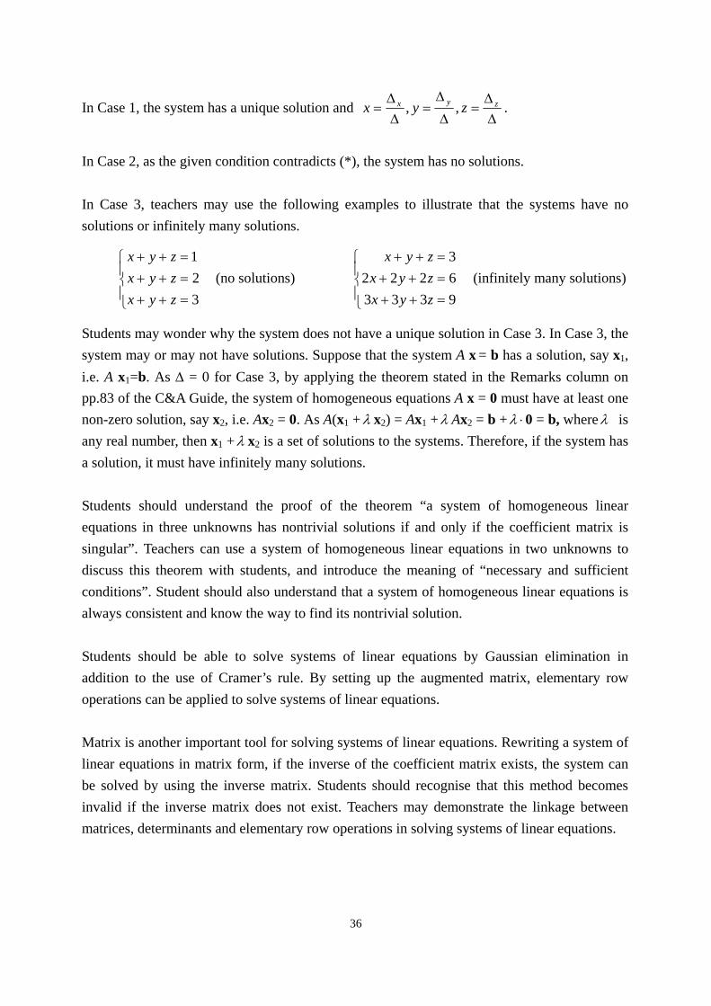
In Case 3, teachers may use the following examples to illustrate that the systems have no
solutions or infinitely many solutions.
3
2
1
zyx
zyx
zyx
(no solutions)
9333
6222
3
zyx
zyx
zyx
(infinitely many solutions)
Students may wonder why the system does not have a unique solution in Case 3. In Case 3, the
system may or may not have solutions. Suppose that the system A x = b has a solution, say x1,
i.e. A x1=b. As = 0 for Case 3, by applying the theorem stated in the Remarks column on
pp.83 of the C&A Guide, the system of homogeneous equations A x = 0 must have at least one
non-zero solution, say x2, i.e. Ax2 = 0. As A(x1 + x2) = Ax1 + Ax2 = b + 0 = b, where is
any real number, then x1 + x2 is a set of solutions to the systems. Therefore, if the system has
a solution, it must have infinitely many solutions.
Students should understand the proof of the theorem “a system of homogeneous linear
equations in three unknowns has nontrivial solutions if and only if the coefficient matrix is
singular”. Teachers can use a system of homogeneous linear equations in two unknowns to
discuss this theorem with students, and introduce the meaning of “necessary and sufficient
conditions”. Student should also understand that a system of homogeneous linear equations is
always consistent and know the way to find its nontrivial solution.
Students should be able to solve systems of linear equations by Gaussian elimination in
addition to the use of Cramer’s rule. By setting up the augmented matrix, elementary row
operations can be applied to solve systems of linear equations.
Matrix is another important tool for solving systems of linear equations. Rewriting a system of
linear equations in matrix form, if the inverse of the coefficient matrix exists, the system can
be solved by using the inverse matrix. Students should recognise that this method becomes
invalid if the inverse matrix does not exist. Teachers may demonstrate the linkage between
matrices, determinants and elementary row operations in solving systems of linear equations.
37
Learning Unit Learning Objective Time
Algebra Area
Vectors
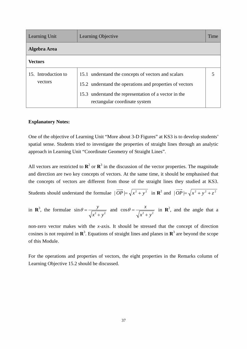
15. Introduction to
vectors
15.1 understand the concepts of vectors and scalars
15.2 understand the operations and properties of vectors
15.3 understand the representation of a vector in the
rectangular coordinate system
5
Explanatory Notes:
One of the objective of Learning Unit “More about 3-D Figures” at KS3 is to develop students’
spatial sense. Students tried to investigate the properties of straight lines through an analytic
approach in Learning Unit “Coordinate Geometry of Straight Lines”.
All vectors are restricted to R2 or R3 in the discussion of the vector properties. The magnitude
and direction are two key concepts of vectors. At the same time, it should be emphasised that
the concepts of vectors are different from those of the straight lines they studied at KS3.
Students should understand the formulae 22|| yxOP in R2 and 222|| zyxOP
in R3, the formulae 2 2
siny
x y
and
2 2cos
x
x y
in R2, and the angle that a
non-zero vector makes with the x-axis. It should be stressed that the concept of direction
cosines is not required in R3. Equations of straight lines and planes in R3 are beyond the scope
of this Module.
For the operations and properties of vectors, the eight properties in the Remarks column of
Learning Objective 15.2 should be discussed.
38
Learning Unit Learning Objective Time
Algebra Area
Vectors
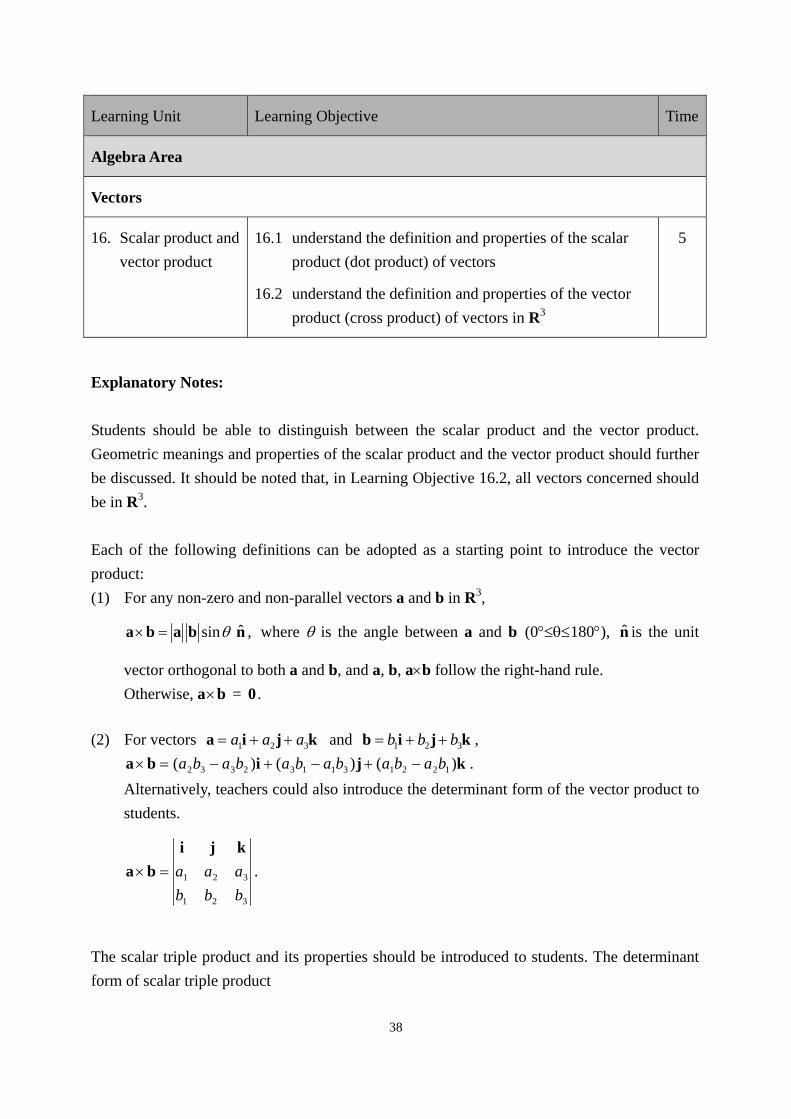
16. Scalar product and
vector product
16.1 understand the definition and properties of the scalar
product (dot product) of vectors
16.2 understand the definition and properties of the vector
product (cross product) of vectors in R3
5
Explanatory Notes:
Students should be able to distinguish between the scalar product and the vector product.
Geometric meanings and properties of the scalar product and the vector product should further
be discussed. It should be noted that, in Learning Objective 16.2, all vectors concerned should
be in R3.
Each of the following definitions can be adopted as a starting point to introduce the vector
product:
(1) For any non-zero and non-parallel vectors a and b in R3,
ˆsina b a b n , where is the angle between a and b (0180), n̂ is the unit
vector orthogonal to both a and b, and a, b, ab follow the right-hand rule.
Otherwise, ab = 0 .
(2) For vectors kjia 321 aaa and kjib 321 bbb ,
kjiba )()()( 122131132332 babababababa .
Alternatively, teachers could also introduce the determinant form of the vector product to
students.
321
321
bbb
aaa
kji
ba .
The scalar triple product and its properties should be introduced to students. The determinant
form of scalar triple product

39
321
321
321
)(
ccc
bbb
aaa
cba , where 1 2 3a i j ka a a , 1 2 3b i j kb b b and
1 2 3c i j kc c c should also be introduced.
The properties of determinants can be used to prove the two properties of scalar triple products
(a b) c = a (b c) and (a b) c = (b c) a = (c a) b. The geometric meaning of
a (b c) can be regarded as “the base area of a face of the parallelepiped times its
corresponding height”. In other words, the scalar triple product is the volume of a
parallelepiped.
40
Learning Unit Learning Objective Time
Algebra Area
Vectors
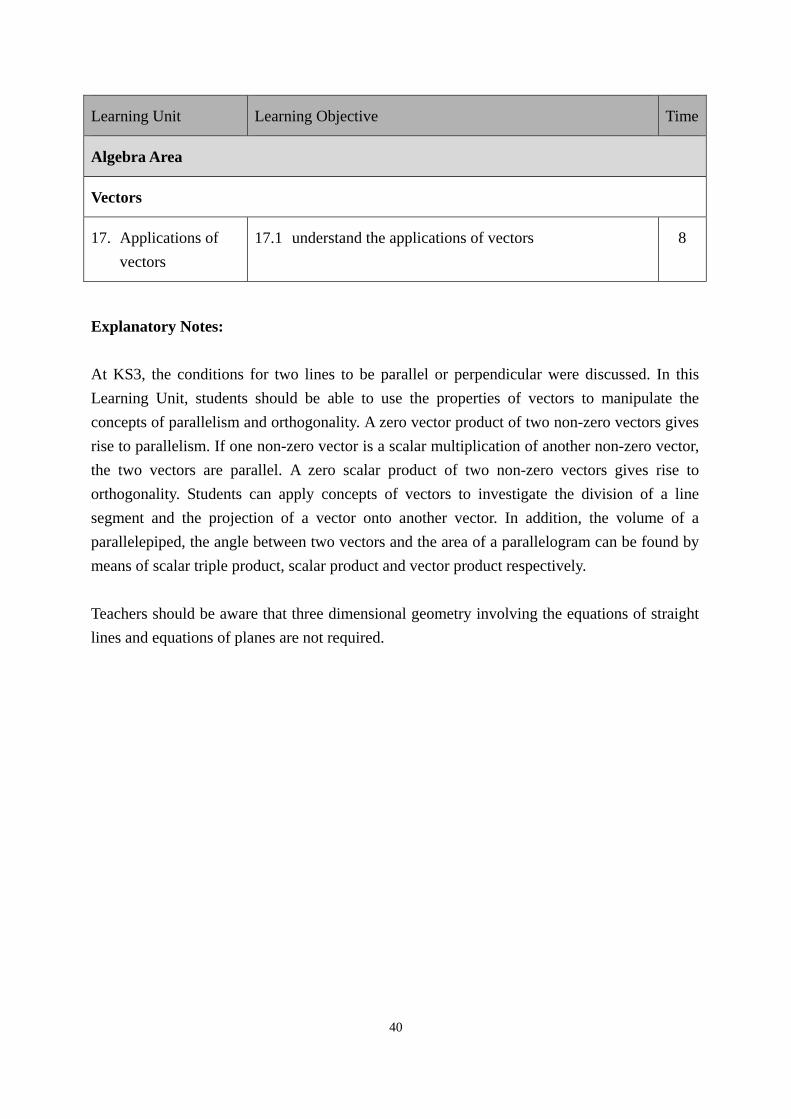
17. Applications of
vectors
17.1 understand the applications of vectors 8
Explanatory Notes:
At KS3, the conditions for two lines to be parallel or perpendicular were discussed. In this
Learning Unit, students should be able to use the properties of vectors to manipulate the
concepts of parallelism and orthogonality. A zero vector product of two non-zero vectors gives
rise to parallelism. If one non-zero vector is a scalar multiplication of another non-zero vector,
the two vectors are parallel. A zero scalar product of two non-zero vectors gives rise to
orthogonality. Students can apply concepts of vectors to investigate the division of a line
segment and the projection of a vector onto another vector. In addition, the volume of a
parallelepiped, the angle between two vectors and the area of a parallelogram can be found by
means of scalar triple product, scalar product and vector product respectively.
Teachers should be aware that three dimensional geometry involving the equations of straight
lines and equations of planes are not required.

41
Learning Unit Learning Objective Time
Further Learning Unit
18. Inquiry and
investigation
Through various learning activities, discover and construct
knowledge, further improve the ability to inquire,
communicate, reason and conceptualise mathematical
concepts
10
Explanatory Notes:
This Learning Unit aims at providing students with more opportunities to engage in the
activities that avail themselves of discovering and constructing knowledge, further improving
their abilities to inquire, communicate, reason and conceptualise mathematical concepts when
studying other Learning Units. In other words, this is not an independent and isolated Learning
Unit and the activities may be conducted in different stages of a lesson, such as motivation,
development, consolidation or assessment.
42
Acknowledgements
We would like to thank the members of the following Committees and Working Group for their invaluable comments and suggestions in the compilation of this booklet. CDC Committee on Mathematics Education CDC-HKEAA Committee on Mathematics Education (Senior Secondary) CDC-HKEAA Working Group on Senior Secondary Mathematics Curriculum (Module 2)