Embed Size (px)
Citation preview

PU/NE-07-06
TASK ORDER 10
VOID FRACTION IN LARGE DIAMETER PIPES:LITERATURE SEARCH FOR EXISTING DATABASE AND
CORRELATIONS
by
M. Ishii, S. S. Paranjape, P. H. Sawant, and B. Ozar
Prepared forU.S. Nuclear Regulatory Commission
Two White Flint North11545 Rockville PikeRockville, MD 20852
PURDUEUNIVERSITY
March 2007
PURDUE UNIVERSITYSCHOOL OF NUCLEAR ENGINEERING
PURDUE UNIVERSITYSCHOOL OF NUCLEAR ENGINEERING
PU/NE-07-06
TASK ORDER 10
VOID FRACTION IN LARGE DIAMETER PIPES:LITERATURE SEARCH FOR EXISTING DATABASE AND
CORRELATIONS
M. Ishii, S. S. Paranjape, P. H. Sawant, and B. Ozar
Prepared forU.S. Nuclear Regulatory Commission
Two White Flint North11545 Rockville PikeRockville, MD 20852
School of Nuclear Engineering, 400 Central Drive,West Lafayette, IN 47907, USATel: 765-494-4587; Fax: 765-494-9570

ACKNOWLEDGEMENTS
This work was performed at Purdue University under the auspices of the U.S.
Nuclear Regulatory Commisssion (NRC), Office of Nuclear Regulatory Research,
through the Institute of Thermal-Hydraulics. The authors would like to express their
gratitude to Joseph Kelly, Shawn Marshall, Stephen Bajorek, Jack Rosenthal, and Joseph
Staudenmeier, and other staff of the NRC for their support on the project.
ii
TABLE OF CONTENTS
Page
LIST OF FIGURES............................................................................. IV
LIST OF TABLES............................................................................... V
NOMENCLATURE ............................................................................ VI
ABSTRACT.................................................................................. ViII
CHAPTER 1 INTRODUCTION..............................................................1.
CHAPTER 2 EXPERIMENTAL DATABASE............................................... 4
2.1 Hills (1976) Data ......................................................................... 5
2.2 Hashemi et al. (1986) Data ............................................................. 15
2.3 Hall et al. (1988) Data................................................................... 18
2.4 Smith (2002) Data....................................................................... 22
2.5 Hsu et al. (2000) Data................................................................... 27
2.6 Inoue (2001) Data ....................................................................... 30
2.7 Yoneda et al. Data (2000) .............................................................. 34
CHAPTER 3 CORRELATIONS AND PRELIMINARY COMPARISONS............. 36
3.1 Drift Flux Model by Hills (1976)...................................................... 36
3.2 Drift Flux Model by Shipley (1984)................................................... 37
3.3 Drift Flux Model by Clark and Flemnmer (1985) ..................................... 38
3.4 Drift Flux Model by Kataoka and Ishii (1987) ....................................... 40
3.5 Drift Flux Model by Ishii and Kocamustafaogullari (1985)......................... 41
3.6 Drift Flux Model by Hibiki and Ishii (2003).......................................... 44
CHAPTER 4 SUMMARY..................................................................... 45
REFERENCES .................................................................................. 46
APPENDIX..................................................................................... 48
iii

LIST OF FIGURES
Figure Page
Figure 2.1. Schematic of the test section (Hills, 1976) ............................................... 5
Figure 2.2 Schematic of the test section (Hashemi et al., 1986) ............................... 15
Figure 2.3 Schematic of the test section (Hall et al., 1988) ...................................... 18
Figure 2.4 Schematic of the test section (Smith, 2002) ............................................ 22
Figure 2.5 Schematic of the test section (Hsu et al., 2000) ..................................... 27
Figure 2.6 Schematic of the test section (Inoue, 2001) ............................................ 30
Figure 2.7 Schematic of the test section (Yoneda et al., 2000) ................................. 34
Figure 3.1 Comparison of void fraction predicion by Hills (1976) correlation with
H ills (1976) data ..................................................................................... 37
Figure 3.2 Comparison of void fraction predicion by Shipley (1984) correlation
w ith H ills (1976) data ............................................................................. 38
Figure 3.3 Comparison of void fraction predicion by Clark and Flemmer (1985)
correlation with Hills (1976) data ............................................................ 39
Figure 3.4 Comparison of void fraction predicion by Kataoka and Ishii (1987)
correlation with Hills (1976) data .......................................................... 41
Figure 3.5 Comparison of void fraction predicion by Ishii and Kocamustafaogullari
(1985) correlation with Hills (1976) data ............................................... 42
iv

LIST OF TABLES
Table Page
Table 2.1: Hills (1976) Data in Tabulated Format ...................................................... 6
Table 2.2: Hashemi (1986) et al. Data in Tabulated Format .................................... 16
Table 2.3: Hall (1988) et al. Data in Tabulated Format ............................................. 19
Table 2.4: Smith (2002) Data for 4 in diameter in Tabulated Format ....................... 23
Table 2.5: Smith (2002) Data for 6 in diameter in Tabulated Format ....................... 25
Table 2.6: Hsu et al. (2000) Data in Tabulated Format ............................................ 28
Table 2.7: Inoue (2001) Data in Tabulated Format ................................................. 31
Table 2.8: Yoneda et al. (2000) Data in Tabulated Format ..................................... 35
Table 3.1: Drift-flux correlations recommended by Hibiki and Ishii (2003) ............ 43
V
NOMENCLATURE
Co Distribution parameter
D Diameter [in]
Dh, DH Hydraulic diameter [m]
g Acceleration due to gravity [m s-2]
j Total volumetric flux [m/s]
jf Superficial liquid velocity [m/s]
jg Superficial gas velocity [m/s]
N•U Viscosity number
p pressure [Pa.]
Vg Gas velocity [m/s]
vf Liquid velocity [m/s]
vgj Drift velocity (vg -j ) [mis]
v fluid particle velocity [m s-1]
GREEK SYMBOL
a Gas void fraction
P Viscosity [Kg m-'s-1]
p Density [Kg in 3]
a Surface Tension [Kg S-2]
SUBSCRIPTS
f liquid
g gas
SUPERSCRIPTS
+ Nondimensionalized parameter
vi

OPERATORS
(.) Area averaging
((.)) Void weighted area averaging
vii

ABSTRACT
This report provides the literature survey for the research being carried out at
Purdue University as a part of the Task Order 10, under Contract No. NRC-04-03-048
(Thermal Hydraulic Tasks), for U.S. Nuclear Regulatory Commission. The objective of
the research is to collect data base to evaluate the models used to predict the void fraction
especially in the transition region between bubbly/slug and annular/mist regimes in large
diameter pipes. The literature survey is the first part of this program and is aimed to find
the available literature both as experimental database and the correlations that are used
for void fraction prediction in large diameter pipes. A detailed literature survey is carried
out. It is found that most of the experimental database reported in the literature does not
specify the boundary conditions of the problem and the measurement methods very well.
Only those with sufficient information for model evaluation are used in this report. Also,
drift flux correlations for large pipe geometry are cited. A MATLAB code is written in
order to compare the collected database with the correlations. Preliminary comparison
results are provided.
viii

CHAPTER 1 INTRODUCTION
The USNRC's (United States Nuclear Regulatory Commission) system thermal-
hydraulic analysis code TRACE (TRAC RELAP Advanced Computational Engine) is
being developed to provide a best-estimate accident analysis capability for both operating
pressurized and boiling water reactors as well as the next generation of evolutionary
water reactor designs. In partnership with the code development, a comprehensive code
assessment activity has been initiated. Results from these assessments have identified a
code modeling deficiency for the prediction of void fraction in large diameter pipes.
Remediation of this code deficiency has a high priority due to its impact on calculations
for the proposed ESBWR design.
In the ESBWR design, a tall chimney region exists above the reactor core to
provide the gravity head necessary to drive the natural circulation two-phase flow
through the core. For this chimney region, the TRACE code uses the same interfacial
drag models as for 1-D vertical pipes. That is, for the bubbly/slug flow regime, the
Kataoka-Ishii drift flux model for large diameter pipes is converted to an interfacial
friction coefficient. For the annular/mist flow regime, the Wallis annular flow interfacial
friction model is used for the liquid film. When entrained droplets are predicted to exist,
the drop volume fraction is estimated and the associated interfacial drag is added to that
for the liquid film. For the transition region between these two regimes, TRACE uses a
simple power-law weighting scheme to provide a continuous and smooth transition.
Two sources of data were identified to assess these models for hydraulic
diameters of about the same size as the ESBWR chimney: pool data (Wilson and Carrier
bubble rise tests) and the Ontario-Hydro transient upflow tests. In the assessment against
the pool data, the TRACE code performed quite well up to void fractions of about 50-
60%. This is not surprising as these tests were included in the data base used to develop
I

the Kataoka-Ishii drift flux model. However, for the large pipe data, there were a few data
points in the void fraction range 60-80% and for which TRACE significantly under-
predicted the void fraction.
For the Ontario-Hydro transient upflow tests, two deficiencies were observed in
the TRACE assessment calculation. First, similar to the predictions for the pool data
mentioned above, the TRACE calculated void fractions compared well up to a value of
about 50%. For higher void fractions, however, TRACE progressively began to under-
predict the void fraction until for a data value of 78%, the TRACE calculated value was
only 67%. To put this into perspective, this means that TRACE could over-predict the
liquid inventory in the chimney region by 50% thereby providing a non-conservative
initial condition for a LOCA analysis.
A second potential modeling deficiency was observed at the Ontario-Hydro
transient test as the mass flux decreased and the quality approached 90%. In the data, the
void fraction was reported to be near unity, whereas in the TRACE calculation, the value
was only 80%. This would appear to indicate that TRACE significantly under-predicts
the interfacial shear in the transition region between bubbly/slug and annular/mist
regimes. While this conclusion is consistent with the observation from the pool data
comparisons, it is tentatively due to the uncertain boundary conditions of the Ontario-
Hydro tests for the high quality conditions.
In summary, assessment of the TRACE code has revealed a significant under-
prediction for the void fraction in large diameter pipes in the transition region between
the bubbly/slug and annular/mist regimes. While the existing data is sufficient to indicate
the existence of a deficiency in the TRACE interfacial drag model, there is not enough
data to permit the selection or development of a new model to address this deficiency.
Consequently, this task is being put in place both to generate the needed data and to
perform the model selection/.development necessary to improve TRACE's ability to
predict void fraction in large diameter pipes.
In order to be able to develop new models, existing experimental and theoretical
work needs to be assessed. In Chapter 2 of this study existing experimental work, which
can be used in model development and assessment is introduced. Simple experimental
2

schematics with important facility components and key dimensions are provided along
with database. Some highlights about these experimental works are also given.
Correlations, which are used to estimate the interfacial shear forces and bubble
distribution parameter, are presented in Chapter 3. Preliminary comparisons are
performed between the data base and these correlations and are provided in this chapter.
Finally, the whole work is summarized in Chapter 4. Also, a MATLAB code is written in
order to compare the experimental database with the correlations. A brief description of
how this software works and also the scripts of this software are given in the Appendix.
3

CHAPTER 2 EXPERIMENTAL DATABASE
In this chapter, an experimental database on void fraction measurements in large
diameter pipe is presented. The database includes seven different data sets. The range of
diameter covered is 101.6mm (4 in.) to 304.8mm (12 in.). The database includes air-
water and steam water experiments. Information about the experimental facility used for
the obtaining data, boundary conditions and void fraction measurements are summarized
in this chapter.
4
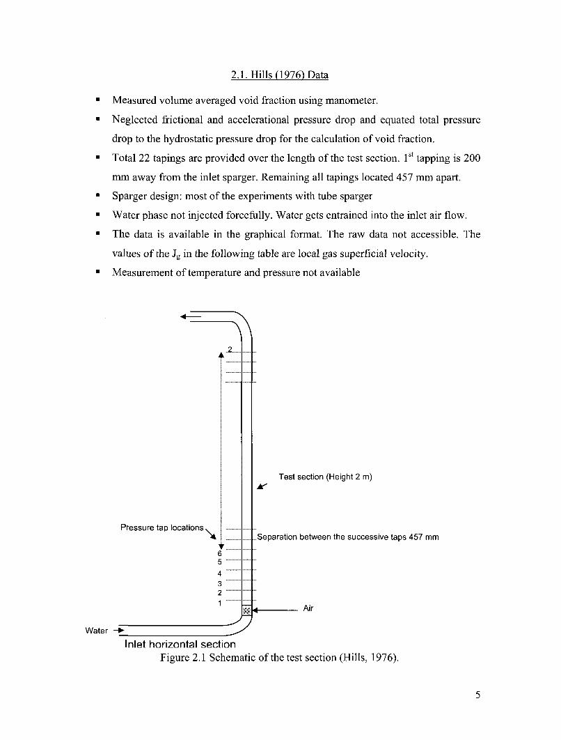
2.1. Hills (1976) Data
" Measured volume averaged void fraction using manometer.
" Neglected frictional and accelerational pressure drop and equated total pressure
drop to the hydrostatic pressure drop for the calculation of void fraction.
" Total 22 tapings are provided over the length of the test section. 1 st tapping is 200
mm away from the inlet sparger. Remaining all tapings located 457 mm apart.
" Sparger design: most of the experiments with tube sparger
" Water phase not injected forcefully. Water gets entrained into the inlet air flow.
" The data is available in the graphical format. The raw data not accessible. The
values of the Jg in the following table are local gas superficial velocity.
" Measurement of temperature and pressure not available
4-
.2.
Pressure tap locations ..........
65.432.
1......
Test section (Height 2 m)
Separation between the successive taps 457 mm
Air
Water --*0ý
Inlet horizontal sectionFigure 2.1 Schematic of the test section (Hills, 1976).
5

Table 2. 1: Hills (1976) Data in Tabulated FormatTitleAuthorYearSource
The Operation of a Bubble Column at High Tthroughputs 1. Gas Holdup Measurements-Hills, J. H.
1976The Chemical Engineering Journal, 12 (1976) pp- 89-99
Air-waterFluid System
Test Section GeometryDiameterLengthInjector specs
MeasurementMeasured parametersInstrumentsMeasurement location
Tube0.15m10.5 mTube Sparger, Run No 109 60 hole sparger
Volume average void fraction, air and water flow rateManometer fro the void fraction measurementNA
Sr. No. T P J9 [ f void L/Dh Flow regime Comments1 ? atm tm/s] [mls] [-]2? 0.04 0 0.121212 ? N/A Jg is local3 ? 0.04 0 0.117647 ? N/A Jg islocal4 ? 0.05 0 0.142857 ? N/A Jg is local5 ? 0.05 0 0.138889 ? N/A Jg is local6 ? 0.05 0 0.131579 ? N/A Jg is local7-? 0.05 0 0.128205 ? N/A Jg is local8 ? 0.06 0 0.146341 ? N/A Jg is local9 ? 0.06 0 0.142857 ? N/A Jg is local
10 ? 0.07 0 0.170732 ? N/A Jg is local11?• 0.07 0 0.159091 ? N/A Jg is local12 ? 0.08 0 0.186047 ? N/A Jg is local13 ? 0.08 0 0.177778 ? N/A Jg is local14 ? 0.08 0 0.173913 ? N/A Jq is local15 ? 0.08 0 0.170213 ? N/A Jg is local16 ? 0.08 0 0.166667 ? N/A Jg is local17 ? 0.09 0 0.183673 ? N/A Jg is local18 ? 0.1 0 0.208333 ? N/A Jg is local19 ? 0.1 0 0.2 ? N/A Jg is local20 ? 0.1 0 0.192308 ? NIA Jg is local
21 ? 0.11 0 0.215686 ? N/A Jg is local22? 0.11 0 0.207547 ? N/A Jg is local23,? 0.12 0 0.226415 ? N/A Jg is local24 ? 0.12 0 0-218182 ? N/A Jg is local25 ? 0.13 0 0.22807 ? NIA Jg is local
6

Table 2.1 continued26 ? 0.13 0 0.220339 ? NIA J9 is local27 ? 0.13 0 0.216667 ? NIA Jg isNloca28 ? 0.14 0 0.237288 ? NIA J7 is local29 ? 0.14 0 0.215385 ? N/A J_ is local30 ? 0.14 0 0.212,121 ? NA Jg isNlocal31 ? 0_15 0 0245902 ? NA JN is local32 ? 0.15 0 0.238095 ? NIA Jg islocal33 ? 0.15 0 0.227273 ? NIA J_ is local34 ? 0.15 0 0.220588 ? NIA J9 is local35 ? 0.16 0 0.25 ? NIA J9 is local36 ? 0.17 0 0.269841 ? N/A Jg ks local
37 ? 0.17 0 0.261538 ? N/AJq islocal38 ? 0.17 0 0.253731 ? NIA J_ is local39 ? 0.17 0 0.242857 ? I NIA J_ is local40 ? 0.18 0 0.272727 ? I N/A Jg is local41 ? 0.18 0 0.268657 ? N/A Jg is local42 ? 0.18 0 0.264706 ? NIA J9 is local43 ? 0.18 0 0.257143 ? WA JA is local44 ? 0.18 0 0.25 ? N/A Jg is local45 ? 0.19 0 0.267606 ? N/A Jg is local46 ? 0.2 0 0.298507 ? N/A Jg is local47 ? 0.2 0 0.285714 ? N/A Jg is local48 ? 0.2 0 0273973 ? N/A J9 is local49 ? 0.2 0 0.27027 ? N/A Jg is local50 ? 0.21 0 0.287671 ? N/A Jg is local51 ? 0.21 0 0.28 ? N/A J9 is local52 ? 0.22 0 0.309859 ? N/A J9 is local53 0.22 0 0.305556 ? N/A Jg is local54 ? 0.22 0 0.30137 ? NIA Jg is local55 ? 0.22 0 0.297297 ? NIA J9 is local56 ? 0.22 0 0.293333 ? N/A J9 is local57 ? 0.22 0 0.289474 ? N/A J9 is local58 ? 0.23 0 0.306667 ? NIA Jg is local59 ? T0.23 0 0.294872 ? N/A 39 is local60 ? 1 0.24 0 0.333333 ? N/A Jq is local61 ? 0.24 0 0.328767i? N/A J9 is local62 ? 0.24 0 0.307692 ? N/A J3 is local63? 0.25 0 0.333333 ? N/A Jg is local64 ? 0.25 0 0.316456 ? N/A Jg is local65 ? 0.26 0 0.337662 ? N/A Jg is local66 ? 0.27 0 0.3461541? N/A Jg is local671? 0.27 0 0.33751? NIA Jg is local681? 1 0.27 0 0.3068181? N/A Jg is local
7

Table 2.1 continued69 ? 0.28 0 035 ? NIA Jg is local70 ? 0.28 0 0341463 ? _ NVA Jg is local71 ? 0.28 0 0.318182 ? N/A Jg is local72 ? 0.29 0 0.353659 ? N/A Jg is local73 ? 0.29 0 0.318681 ? N/A Jg is local74 ? 0.3 0 0.32967 ? N/A Jg is local75 ? 0.31 0 0.333333 ? N/A Jg is local76 ? 0.33 0 0.347368 ? N/A Jq is local77 ? 0.34 0 0.354167 ? _N/A Jq is local78 ? 0.35 0 0.360825 ? NIA Jq is local79 ? 0.36 0 0.367347 ? N/A Jg is local80 ? 0.37 0 0.373737 ? N/A Jq is local81 ? 0.38 0 0.38 ? N/A J9 is local82 ? 0.38 0 0.351852 ? N/A Jg is local83? 0.39 0 0.375 ? N/A Jg is local84 ? 0.4 0 0.380952 ? N/A Jg is local85 0.4 0 0.373832 ? N /A Jg is local86 ? 0.41 0 0.383178 ? N/A Jq is local87 ? 0.41 ( 0.37963 ? NIA Jg is local88 ? 0.42 0 0.381818 ? N/A Jg is local89 ? 1 043 0 0.40566 ? N/A Jg is local90? 0.43 0 0.387387 ? N/A Jg is local91 ? 0.44 0 0.392857 ? N/A Jq is local92 ? 0.44 0 0.385965 ? NIA Jg is local93 ? 0.45 0 0.38793t1 ? N/A Jg is local94 ? 0.46 0 0.396552 ? N/A J9 is local95 ? 0.47 0 0.408696 ? N/A Jg is local96 ? 1 0.48 0 0.417391 ?_ N/A Jg is local97 ? 0.49 0 0.418803 ? N/A Jg is local98 ? 0.5 0 0423729 ? NIA Jg is local99 ? 0.51 0 0.439655 ? N/A Jg is local
100 ? 0 _52 0 0.440678 ? N/A Jg is local101 ? 0.53 0 0.430894 ? N/A Jg is local102 ? 0.55 0 0.436508 ? N/A Jg is local1030.56 ? 10-6 0 0.440945 ? N/A Jg is local104 ? 0.58 0 0.453125 ? N/A Jg is local105 ? 0.59 0 0.453846 ? NIA Jg is local106 ? 0.08 0.1 0.166667 ? N/A Jg is local107 ? 0.08 0.1 0.156863 ? N/A Jg is local108 ? 0.08 0.1 0.153846 ? NIA Jg is local109 ? 0.09 0.1 0.166667 ? N/A Jg is local1 0.1 0.1 0.181818 ? WNA Jg is local111? 0111 0.1 0.196429 ? N/A Jg is local
8

Table 2.1 continued
155 ? 0-38 0.1 0.342342 ? N/A Jg is local156 ? 0.39 0.1 0.357798 ? N/A Jg is local157 ? 0.4 0.1 0.37037 ? NIA Jg is local158 ? 0.4 0.1 0.366972 ? NIA Jg is local159 ? 0.41 0.1 0.383178 ? N/A Jg is local160 ? 0.42 0.1 0.371681 ? N/A Jg is local161 ? 0.43 0.1 0.373913 ? N/A Jg is local162 ? 0.44 0.1 0.376068 ? NIA Jg is local163 ? 0.45 0.1 0.391304 ? NIA Jg is local164 ? 0.47 0.1 0.401709 ? N/A Jg is local165 ? 0.47 0.1 0.398305 ? NIA Jg is local166 ? 0.48 0.1 0.4 ? N/A J9 is local167 ? 0.49 0.1 0.401639 ? N/A Jg is local168 ? 0.5 0.1 0.4 ? N/A Jg is local169 ? 0.51 0.1 0.398438 ? N/A Jg is local170 ? 0.52 0.1 0.419355 ? N/A Jg is local171 ? 0.53 0.1 0.420635 ? N/A Jg is local172 ? 0.53 0.1 0.410853 ? N/A Jg is local173 ? 0.54 0.1 0.425197 ? N/A Jg is local174 ? 0.55 0.1 0.44 ? NIA Jg is local175 ? 0.55 0.1 0.423077 ? NIA Jg is local176 ? 0.56 0.1 0.424242 ? NIA Jg is local177 ? 0.57 0.1 0.425373 ? N/A Jg is local178 ? 0.58 0.1 0.42963 ? N/A Jg is local179 ? 0.6 0.1 0.434783 ? N/A Jg is local180 ? 0.61 0.1 0.442029 ? N/A Jg is local181 ? 0.62 0.1 0.439716 ? NIA Jg is local182 ? 0.06 0.25 0.105263 ? N/A Jg is local183 ? 0.06 0.25 0.103448 ? N/A Jg is local184 ? 0.06 0.25 0.101695 ? NIA Jg is local185 ? 0.06 0.25 0.1 ? N/A Jg is local186 ? 0.08 0.25 0.140351 ? N/A Jg is local187 ? 0.08 0.25 0.137931 ? N/A Jg is local188 ? 0.08 0.25 0.135593 ? N/A Jg is local189 ? 0.08 0.25 0.119403 ? N/A Jg is local190 ? 0.09 0.25 0.147541 ? N/A Jg is local191 ? 0.09 0.25 0.145161 ? N/A Jg is local192 ? 0.09 0.25 0.142857 ? N/A Jg is local193 ? 009 0.25 0.134328 ? N/A Jg is local194 ? 0.09 0.25 0.132353 ? N/A Jg is local195 ? 0.1 0.25 0.144928 ? NIA Jg is local196 ? 0.1 0.25 0.142857 ? N/A Jg is local197 ? 0.1 0.25 0.138889 ? N/A Jg is local
9

Table 2.1 continued198 ? 0.11 0-25 0.150685 ? NIA Jg is local199 ? 0.11 0-25 0.146667 ? N/A Jg islocal200 ? 0.12 0ý25 0.164384 ? N/A Jg is local201 ? 0.12 0.25 0.16 ? N/A Jg is local202 ? 0.12 0-25 0.157895 ? N/A Jg is local203 ? 0.13 0-25 0.178082 ? N/A Jg is local204 ? 0-13 0.25 0.173333 ? N/A Jg is local205 ? 0.13 0.25 0.168831 ? N/A Jg is local206 ? 0.14 0.25 0.179487 ? N/A Jg is local207 ? 0.14 0.25 0.175 ? N/A Jg is local208 ? 0.15 0.25 0.194805 ? N/A Jg is local209 ? 0.15 0.25 0.1875 ? N/A Jg is local210 ? 0.15 0.25 0.185185 ? NIA Jg is local211 ? 0.15 0.25 0.182927 ? N/A Jg is local212 ? 0.15 0.25 0.178571 ? NIA Jg is local213 ? 0.16 0.25 0-188235 ? N/A Jg is local214 ? 0.18 0.25 0. 2 09 3 0 2 ? N/A Jg is local215 ? 0.18 0.25 0.206897 ? NIA Jg is local216 ? 0.19 0.25 0.218391 ? N/A Jg is local217 ? 0.2 0.25 0.227273 ? NIA J 9 is local218 ? 0.2 0.25 0.222222 ? NIA Jg is local219 ? 0.22 0.25 0.244444 ? N/A Jg is local220 ? 0.22 0.25 0.241758 ? N/A Jg is local221 ? 0.23 0.25 0.242105 ? N/A Jg is local222 ? 0.23 0.25 0.237113 ? N/A Jg is local223 ? 0.25 0.25 0.257732 ? NIA Jg is local224 ? 0.26 0.25 0.265306 ? N/A Jg is local225 ? 0.26 0.25 0.26 ? NIA Jg is local226 ? 0.27 0.25 0.267327 ? N/A Jg is local227 ? 0.28 0.25 0.27451 ? NIA Jg is local228 ? 0.28 0.25 0.271845 ? NIA Jg is local229 ? 0.29 0.25 0.278846 ? NIA Jg is local230 ? 0.3 0.25 0.285714 ? N/A Jg is local231 ? 0.31 0.25 0.28972 ? N/A Jg is local232 ? 0.32 0.25 0.296296 ? N/A Jg is local233 ? 0.33 0.25 0.3 ? NIA Jg is local234 ? 0.34 0.25 0.309091 ? N/A Jg is local235 ? 0.1 0.4 0.114943 ? N/A Jg is local236 ? 0.11 0.4 0.127907 ? N/A Jg is local237 ? 0.11 0.4 0.126437 ? N/A Jg is local238 ? 0.11 0.4 0.123596 ? N/A Jg is local239 ? 0.13 0.4 0.146067 ? NIA Jg is local240-? 0.13 0.4 0.142857 ? N/A Jg is local
10

Table 2.1 continued241 ? 0.13 0.4 0.142857 ? NIA Jg is local242 ? 0.14 0.4 0.150538 ? NIA Jg is local243 ? 0.14 0.4 0.148936 ? NIA Jg is local244 ? 0.15 0.4 0.157895 ? NIA Jg is local245 ? 0.15 0.4 0.15625 ? N/A Jg is local246 ? 0.16 0.4 0.163265 ? NIA Jg is local247 ? 1 0.18 0.4 0.168224 ? N/A Jg is local248 ? 0.19 0.4 0.175926 ? N/A Jg is local249 ? 0.2 0.4 0.183486 ? N/A Jg is local250 ? 0.21 0.4 0.190909 ? NIA Jg is local251 ? 0.22 0.4 0.198198 ? N/A Jg is local252 ? 0.22 0.4 0.184874 ? N/A Jg is local253 ? 0.23 0.4 0.20354 ? INA Jg is local254 ? 0.24 0.4 0.208696 ? N/A Jg is local255 ? -0.25 0.4 0.213675 ? N/A Jg is local256 ? 0.25 0.4 0.211864 ? NIA Jg is local257 ? 0.25 0.4 0.208333 ? N/A Jg is local258 ? 0.26 0.4 0.214876 ? N/A Jg is local259 ? 0.27 0.4 0.22314 ? N/A Jg is local260 ? 0.27 0.4 0.219512 ? N/A Jg is local261 ? 0.28 0.4 0.225806 ? N/A J9 is local262 ? 0.29 0.4 0.237705 ? N/A Jg is local263 ? 0.29 0.4 0.230159 ? N/A Jg is local264 ? 0.31 0.4 0.246032 ? N/A Jg is local265 ? 0.32 0.4 0.251969 ? N/A Jg is local266 ? 0.32 0.4 0.246154 ? NIA Jg is local267 ? 0.33 0.4 0.24812 ? N/A Jg is local268 ? 0.34 0.4 0.251852 ? MA Jg is local269 ? 0.35 0.4 0.257353 ? N/A Jg is local270 ? 0.36 0.4 0.266667 ? N/A Jg is local271 ? 0.05 0.5 0.05814 ? NIA Jg is local272 ? 0.05 0.5 0.056818 ? N/A J9 is local273 ? 0.05 0.5 0.054348 ? N/A Jg is local274 ? 0.06 0.5 0.067416 ? N/A Jg is local275 ? 0.06 0.5 0.065217 ? NIA Jg is local276 ? 0.06 0.5 0.06383 ? N/A Jg is local277 ? 0.07 0.5 0.079545 ? N/A Jg is local278 ? 0.14 0.5 0.126126 ? I NIA Jg is local279 ? 0.15 0.5 0.132743 ? INA Jg is local280 ? 0.17 0.5 0.147826 ? N/A Jg is local281 ? 0.17 0.5 0.145299 ? N/A Jg is local282 ? 0.19 0.5 0.161017 ? IN/A Jg is local283 ? 0.2 0.5 0.168067 ? N/A Jg is local
ll

Table 2.1 continued284 0.2 0.5 0.163934 ? N/A Jg is local285 ? 0.21 0.5 0.169355 ? NIA Jg is local286 ? 0.23 0.5 0.181102 ? N/A Jg islocal287 ? 0.25 0.5 0.193798 ? NIA Jg is local288 ? 0.26 0.5 0.206349 ? N/A Jg is local289 ? 0.27 0.5 0.210938 ? NIA Jg is local290 ? 0.27 0.5 0.207692 ? N/A Jg is local291 ? 027 0.5 0.203008 ? N/A Jg is local292 ? 0.28 0.5 0.21374 ? N/A Jo is local293 ? 03 0.5 0.229008 ? NIA Jg is local294 ? 0.3 0.5 0.225564 ? N/A Jg is local295 ? 0.31 0.5 0.22963 ? N/A Jg is local296 ? 0.32 0.5 0.238806 ? NIA Jg is local297 ? 0.32 0.5 0.231884 ? N/A Jg is local298 ? 0.33 0.5 0.24812 ? N/A Jg is local299 ? 0.33 0.5 0.23741 ? NIA Jg is local300 ? 0.34 0.5 0.248175 ? NIA Jg is local301 ? 0.34 0.5 0.246377 ? N/A J9 is local302 ? 0.35 0.5 0.25 ? N/A Jg is local3030.1 ? OA 0 0.25 ? N/A Jg is local304 ? 0.1 0 0.166667 ? N/A Jg is local305 ? 0.2 0 0.333333 ? NIA Jg is local306 ? 0.2 D 0.285714 ? N/A Jg is local307 ? 0.3 0 0.375 ? NIA Jg is local308 ? 0.4 0 0.363636 ? N/A Jg is local309 ? 0.5 0 00454545 ? N/A Jg is local310 ? 0.5 0 0.416667 ? N/A Jg is local311 ? 0.6 0 0.5 ? N/A Jg is local312 ? 0.7 0 0.538462 ? NIA Jg is local313 ? 0.1 0.5 0.090909 ? N/A Jg is local314 ? 0.2 0.5 0.166667 ? NIA Jg is local315 ? 0.2 0.5 0.153846 ? N/A Jgislocal316 ? 0.3 0.5 0.214286 ? NIA Jg is local317 ? 0.4 0.5 0.266667 ? NIA Jg is local318 ? 0.4 0.5 0.25 ? N/A Jg is local319 ? 0.5 0.5 0.3125 ? N/A Jg is local320 ? 0.5 0.5 0.294118 ? N/A Jg is local321 ? 0.6 0.5 0.333333 ? N/A Jg is local322? 0.7 0.5 0.388889 ? N!A J9 is local323 ? 0.7 0.5 0.35 ? N/A Jg is local324 ? 0.8 0.5 0.421053 ? N/A Jg is local325 ? 0.1 1.2 0.055556 ? N/A Jg is local326 ? 0.2 1.2 0.105263 ? _ N/A Jg is local
12
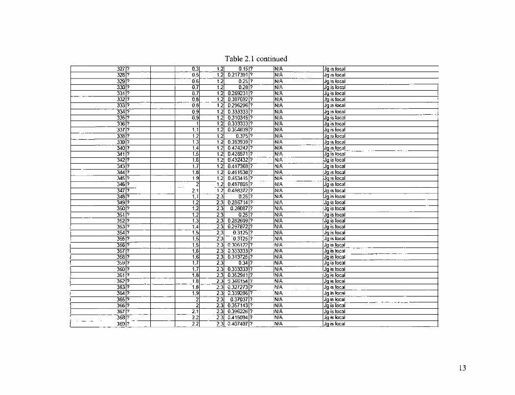
Table 2.1 continued327 ? 0.3 1.2 0.15 ? NIA Jg is local328 ? 0.5 1.2 0.217391 ? N/A Jg is local329 ? 0.6 1.2 0.25 ? NIA Jg is local330 ? 0.7 1.2 0.28 ? N/A Jg is local331 ? 0.7 1.2 0.269231 ? NIA Jg is local332 ? 0.8 1.2 0.307692 ? N/A Jg is local333 ? 0.8 1.2 0.296296 ? N/A Jg is local334 ? 0.9 1.2 0.333333 ? NIA Jg is local335 ? 0.9 1.2 0.310345 ? N/A Jg is local336 ? 1 1.2 0.333333 ? NIA Jg is local337 ? 1.1 1.2 0.354839 ? N/A Jg is local338 ? 1.2 1.2 0.375 ? NIA Jg is local339 ? 1.3 1.2 0393939 ? NIA Jg is local340 ? 1.4 1.2 0-424242 ? N/A Jg is local341 ? 1.5 1.2 0.428571 ? N!A Jg is local342 ? t.6 1.2 0.432432 ? N/A Jg is local343 ? 1.1 1.2 0-447368 ? NIA Jg is local344 ? 1.8 1.2 0.461538 ? NIA Jg is local345 ? 1.9 1.2 0.463415 ? N/A Jg is local346 ? 2 1.2 0.487805 ? IN/A Jg is local347 ? 2.1 1.2 0.488372 ? N/A J9 is local348 ? 1.1 2.3 0.25 ? N/A J1 is local349 ? 1.2 2.3 0.285714 ? NIA Jg is local350 ? 1.2 2.3 0.26087 ? NIA Jg is local351 ? 1.2 2.3 0.25 ? N/A Jg is local352 ? 1.3 2.3 0.282609 ? N/A Jg is local353 ? 1.4 2.3 0.297872 ? IN/A Jg is local354 ? 1.5 2.3 0.3125 ? INIA Jg is local355 ? 1.5 2.3 0.3125 ? N/A Jg is local356 ? 1.5 2.3 0.306122 ? N/A Jg is local357 ? 1.6 2.3 0.333333 ? N/A Jg is local358 ? 1.6 2.3 0.313725 ? NIA J9 is local359 ? 1.7 2.3 0.34 ? NIA Jg is local360 ? 1.7 2.3 0.333333 ? N/A Jg is local361 ? t18 2.3 0.352941 ? _ N/A Jg is local362 ? 1.8 2.3 0.346154 ? N/A Jg is local363 ? 1.8 2.3 0.327273 ? N/A Jg is local364 ? 19 2.3 01339286 ? N/A Jg is local365 ? 2 2.3 0.37037 ? N/A Jg is local366 ? 2 2.3 0357143 ? N/A Jg is local367 ? 2.1 2.3 0.396226 ? iNIA Jg is local368 ? 2-2 2.3 0.415094? N/A Jg is local369 ? 2.2 2.3 0.4074071? N/A Jg is local
13

Table 2.1 continued370 ? 2.2 2.3 0.392857 ? N/A Jg is local371 ? 2.2 2.3 0.385965 ? NYA Jg is local372 ? 2.3 2.3 0.396552 ? NIA Jg is local373 ? 23 2.3 0.389831 ? NIA Jg is local374 ? 2.4 2.3 0.40678 ? N/A Jg is local375 ? 2.5 2.3 0.431034 ? NIA Jg is local376 ? 2.5 2.3 0.403226 ? NIA Jg is local377 ? 2.6 2.3 0.412698 ? NIA Jg is local378 ? 2.7 2.3 0.415385 ? NIA Jg is local379 ? 2.8 2.3 0.444444 ? NIA Jg is local380 ? 2.8 2.3 0.430769 ? N/A Jg is local381 ? 2.9 2.3 0.460317 ? N/A Jg is local382 ? 3 2.3 0.447761 ? N/A Jg is local383 ? 3.1 2.3 0.492063 ? N/A Jg is local384 ? 2.4 2.6 0.363636 ? NIA Jg is local385 ? 2.5 2.6 0.362319 ? NIA Jg is local386 ? 2.6 2.6 0.366197 ? N/A Jg is local387 ? 2.7 2.6 0.391304 ? N/A Jg is local388 ? 2.8 2.6 0.394366 ? N/A Jg is local389 ? 2.8 2.6 0.4 ? N/A Jg is local390 ? 2.9 2.6 0.432836 ? N/A Jg is local391 ? 2.9 2.6 0.42029 ? NIA Jg is local392 ? 3.1 2.6 0.442857 ? N/A Jg is local393 ? 3.2 2.6 0.450704 ? N/A Jg is local3941? 1 3.4 2.6 0.472222 ? N/A Jg is local3951? 1 3.5 2.6 0.479452 ? N/A Jg is local
14

2.2. Hashemi et al. (1986) Data
" The reported gas velocities are nominal and local gas velocities are not available
" It is not clear whether the gamma densitometer measurements are line average or
cross-section average.
" Pressure and temperature not reported.
" At the inlet there is no sparger. There is a horizontal inlet section followed by
elbow and the test section. The air is injected at the exit of the elbow.
Exit
107"
Gamma densitometer locations
7 2 ........ ...... .......
24
Test section
Air inlet
Water-I
Inlet horizontal
Figure 2.2 Schematic of the test section (Hashemi et al., 1986).
15

Table 2.2: Hashemi (1986) et al. Data in Tabulated Format
Title Effect of Diameter and Geometry on Two-phase Flow Regimes ad Carrt-over in a Model PWR Hot LegAuthor Hashemi A., Kim, J. H. and Sursock J. P.Year 1986Source Proceedings of 8th International Heat Transfer Conference, San Francisco. Pp. 2443-2451
Fluid System air-water
Test Section Geometry TubeDiameter 30.5 cm (12 inch)Length 290 cm (114 inch)Injector specs NA
MeasurementMeasured parameters Inlet air and water flow rate, pressure drop, local void fraction (gamma densitometer)Instruments Local Void fraction measured using gamma densitometerMeasurement location Three elevations. From the inlet 24", 72" and 107"
Sr. No. I P ig It <alpha> L/h How regime Comments
I NA NA 0.03 0 0.093 2 NA2 0.03 0 0.126 63 0.03 0 0.128 94 0.06 0 0.129 25 0.06 0 1 0168 6
6 0.06 0 0.173 97 0.12 0 0.232 2
8 0.12 0 0.232 69 0.12 0 0.25 9
10 058 0 0.486 211 0.58 0 0.485 612 0.58 0 0.746 9 Exit effect
13 1A6 0 0.623 214 1.16 0 0.695 61F 1.16 0 0.934 9 Exit effect16 0.01 0.04 0.009 217 0.01 0.04 0.037 618 0.01 0.04 0.031 9 Exit effect19 0.03 0.04 0.066 220 0.03 0.04 0.108 621 0.03 0.04 0.106 9
16
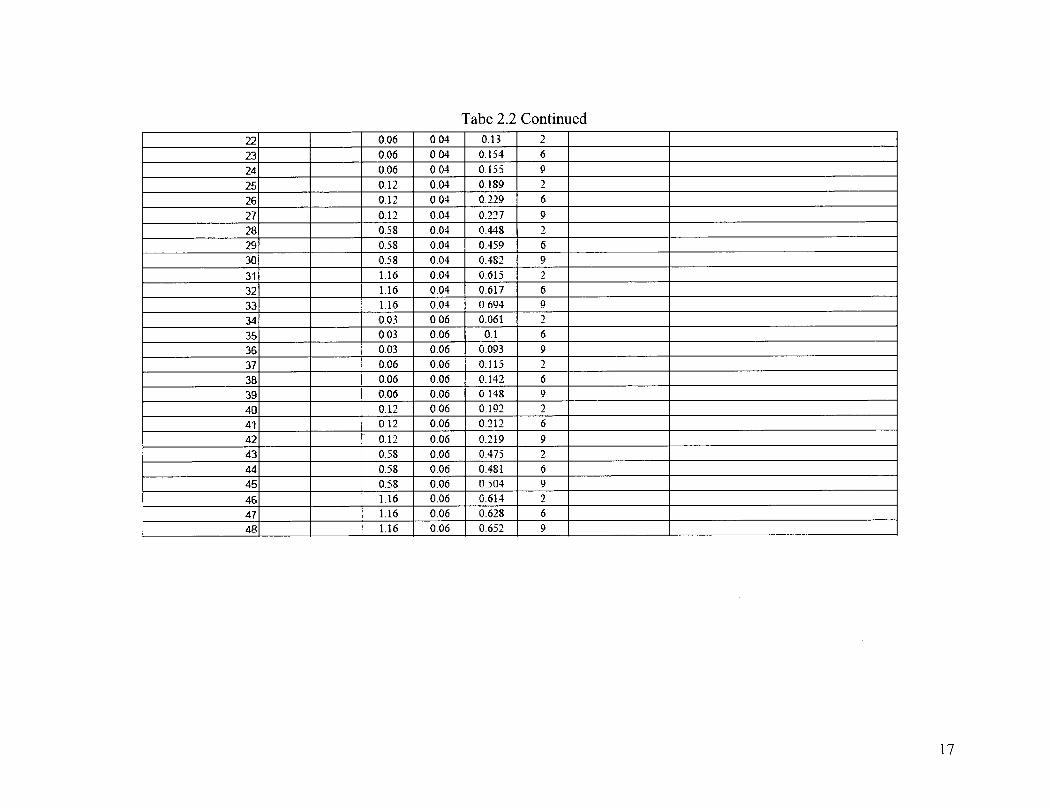
Tabe 2.2 Continued
22 0.06 0.04 0.13 2
23 0.06 0.04 0.154 6
24 0.06 0.04 0.155 9
25 0.12 0.04 0.189 2
26 0.12 0.04 0.229 6
27 0.12 0.04 0.227 9
28 0.58 0.04 0.448 2
29 0.58 0.04 0.459 6
30 0.58 0.04 0.482 9
31 1.16 0.04 0.615 2
32 1.16 0.04 0.617 633 1.16 0.04 0.694 9
34 0.03 0.06 0.061 2
35 0.03 0.06 0.1 6
36 0.03 0.06 0.093 9
37 0.06 0.06 0.115 2
38 0.06 0.06 0.142 6
39 0.06 0.06 0.148 9
40 0.12 0.06 0.192 2
41 0.12 0.06 0.212 6
42 0.12 0.06 0.219 9
43 0.58 0.06 0.475 2
44 0.58 0.06 0.481 6
45 0.58 0.06 0.504 9
46 1.16 0.06 0.614 247 1.16 0.06 0.628 6
48 1.16 0.06 0.652 9
17

2.3. Hall et al. (1988) Data
" Steam is injected into saturated water through a perforated pipe. Then, the mixture
passed through an inclined entrance region and entered the vertical test section
" There is no detailed information available about the state of the two-phase mixture
along the test section. Therefore, properties for the saturation condition (4.4 MPa) are
assumed.
" Mass flow rates for steam and water are given as boundary conditions, therefore, the
superficial velocities are calculated based on densities at saturation temperature and
test section geometry.
" The steam is separated from the mixture via mechanical separation device. The
details of this device are not provided.
" Void measurements in the vertical test section are performed by using differential
pressure sensors over three regions. The volume averaged void fractions for these
three regions are assumed to be at the center of these volumes.
MechanicalSeparation -.Device
Region 3 27.0cm
30.56mRegion 2Tes se tio •.................... 1!109 0chm
Test section10Oc23.5ctm
Region IRegion 1 ~ .................... ..t.
17.0cmf
Entrance "
.. .. ............ 41cm
Figure 2.3 Schematic of the test section (Hall et al., 1988).
18

Table 2.3: Hall (1988) et al. Data in Tabulated Formatitle
•,uthorear
Source
Fluid System
High Pressure Steam/Water Void Fraction Profiles in a Large-Diameter, Vertical Pipe With INHall, W. H., Prueter, W. P_, Thome, T. L. and Wall J. R.
1988conference
Steam-water
Test Section GeometryDiameterLengthInjector specs
MeasurementMeasured parametersInstrumentsMeasurement location
0.1711.09
mixing chamber
volume averageddifferential pressure sensorL/Dh=1.68. 3.26. 4.94
Sr. No. I P(psig) J9 Jr <alpha> LDh Flow regime Comments1 256.07 640.00 0.123 0.021 0.581513 1.680 NIA temperature is based on the sat temp assumption2 256.07 640.00 0.249 0.021 0.522689 1.680 N/A3 256.07 640.00 0.374 0.021 0.537815 1.680 NIA4 256.07 640.00 0.493 0.021 0.594118 1.680 NIA5 256.07 640.00 0.620796 0.021 0_593277 1.680 NIA6 256-07 640.00 0.735 0-021 0.619328 1.680 N/A7 256.07 640.00 0.117042 0.067734 0.440336 1.680 N/A8 256.07 640.00 0.261275 0.067734 0.482353 1.680 NIA9 256.07 640.00 0.385602 0.067734 0.536975 1.680 NtA
10 256.07 640.00 0.503687 0.067734 0.578151 1.680 NIA11 256.07 640.00 0.610378 0.067734 0.577311 1.680 N/A12 256.07 640.00 0.734735 0.067734 0.620168 1.680 N/A13 256.07 640.00 0.122384 0.115 0.397479 1.680 N/A14 256.07 640.00 0.248 0-115 0.494958 1.680 N/A15 256.07 640.00 0.373087 0.115 0.522689 1.680 NIA16 256.07 640.00 0.495357 0.115 0.563866 1.680 NIA17 256.07 640.00 0.61975 0.115 0.593277 1.680 N/A18 256.07 640.00 0.733764 0.115 0.591597 1.680 N/A19 256.07 640.00 0.118 0.162215 0.239496 1.680 N/A20 256.07 640.00 0.248 0.162215 0.368908 t.680 N/A21 256.07 640.00 0.377522 0.162215 0.426891 1.680 N/A22 256.07 640.00 0.496546 0.162215 0.509244 1.680 NIA23 256.07 640.00 0.621991 0.162215 0.536134 1.680 N/A24 256.07 640.00 0.738088 0.162215 0.537815 1.680 N/A25 256.07 640.00 0.124 0.208 0.283193 1.680 NAIA
19
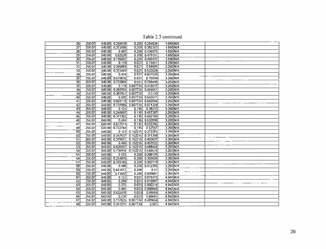
Table 2.3 continued26 256.07 640.00 0.255518 0.208 0.284034 1.680 N/A27 256.07 640.00 0,372408 0.208 0.382353 1.680 N/A28 256.07 640.00 0.487 0.208 0.436975 1.680 N/A29 256.07 640.00 0.62528 0.208 0.478151 1.680 N/A30 256.07 640.00 0.738207 0.208 0.492437 1.680 N/A31 256.07 640.00 0.119 0.021 0.74041 3.260 N/A32 256.07 640.00 0.246868 0.021 0.58805 3.260 N/A33 256.07 640.00 0.372449 0.021 0.522529 3.260 NIA34 256.07 640.00 0.494 0.021 0.631526 3.260 NIA35 256.07 640.00 0.619835 0.021 0.70594 3.260 NIA36 256.07 640.00 0.733004 0.021 0.758498 3.260 NIA37 256.07 640.00 0.119 0.067734 0.415017 3.260 N/A38 256.07 640.00 0.260355 0.067734 0.491041 3.260 N/A39 256.07 640.00 0.383957 0.067734 0.5,132 3.260IN/A40 256.07 640.00 0.500 0.067734 0.545511 3.260 N/A41 256.07 640.00 0.608119 0.067734 0.555944 3.260 N/A42 256.07 640.00 0.737995 0.067734 0.571329 3.260 N/A43 256.07 640.00 0.121 0.115 0.38213 3.260 NIA44 256.07 640.00 0.246697 0.115 0.457387 3.260 N/A45 256.07 64000 0.371362 0.115 0.492186 3.260 N/A46 256.07 640.00 0.494 0.115 0.532896 3.260 N/A47 256.07 640.00 0.617513 0.115 0.532295 3.260 N/A48 256.07 640.00 0.732764 0.115 0.57557 3.260 NIA49 256.07 640.00 0.121 0.162215 0.273385 3.260 N/A50 256.07 640.00 0.247632 0.162215 0.371398 3.260 N/A51 256.07 640.00 0.378577 0.162215 0.403637 3.260 N/A52 256.07 640.00 0.495 0.162215 0.457022 3.260 N/A53 256.07 640.00 0.620597 0.162215 0.488444 3.260 N/A54 256.07 640.00 0.736918 0.162215 0.548574 3.2601N/A55 256.07 640.00 0.123 0.208 0.296135 3.260 N/A56 256.07 640.00 0.254876 0.208 0.305609 3.260 NIA57 256.07 640.00 0.370185 0.208 0.392719 3.260 N/A58 256.07 640.00 0.486 0.208 0.412385 3.260 N/A59 256.07 640.00 0.621672 0.208 0.51 3.260 N/A60 256.07 640.00 0.73582 0.208 0.509801 3.260 N/A61 256.07 640.00 0.121 0.021 0.879373 4.940 N/A62 256.07 640.00 0250 0.021 0.910997 4.940 N/A63 256.07 640.00 0.375 0.021 0.850214 4.940 N/A64 256.07 640.00 0.495 0.021 0.880848 4.940 N/A65 256.07 640.00 0.622478 0.021 0.89568 4.940 N/A66 256.07 640.00 0.734 0.021 0.89487 4.940 N/A67 256.07 640.00 0.117625 0.067734 0.409858 4.940 N/A68 256.07 640.00 0.261274 0.067734 0.501 4.940 N/A
20

Table 2.3 continued69 256.07 640.00 0.385145 0.067734 0.591 4.940 N/A70 256.07 640.00 0.501729 0.067734 0.607 4.940 N/A71 256.07 640.00 0609986 0.067734 0.711 4.940 N/A72 256.07 640.00 0.738021 0.067734 0.715 4.940 NIA73 256.07 640.00 0.120748 0.115 0.316 4.940 NIA74 256.07 640.00 0.247 0.115 0.409 4.940 N/A75 256.07 640.00 0.370572 0.115 0.437 4.940 NIA76 256.07 640.00 0.494443 0.115 0.486 4.940 N/A77 256.07 640.00 0.621437 0.115 0.531 4.940 NIA78 256.07 640.00 0.733857 0.115 0.561 4.940 N/A79 256.07 640.00 0.120 0.162215 0.117 4.940 NIA80 256.07 640.00 0.250 0.162215 0.238 4.940 N/A81 256.07 640.00 0.376818 0.162215 0.300 4.940 N/A82 256.07 640.00 0.496525 0.162215 0.391 4.940 N/A83 256.07 640.00 0.62456 0.162215 0.424 4.940 N/A84 256.07 640.00 0.740103 0.162215 0.467 4.940 N/A85 256.07 640.00 0.126 0.208 0.114 4.940 N/A86 256.07 640.00 0.255028 0.208 0.146 4.940 N/A87 256.07 640.00 0.371613 0.208 0.224 4.940 NIA88 256.07 640.00 0.489 0.208 0.316 4.940 NIA89 256.07 640.00 0.628723 0.208 0.392 4.940 N/A90 256.07 640.00 0.739062 0.208 0.423 4.940 NIA
21

2.4. Smith (2002) Data
" Air is injected through porous spargers
" Pressure correction is used while calculating the superficial gas velocity for each
probe location
" Local void fraction measurements are taken by an optical probe in the radial direction
and area-averaged through the cross sectional area
" Inlet liquid temperature is not provided numerically but it is mentioned to be at room
temperature.
D=101.6mmL1= 508mmL2= 2032mmL 3= 3048mm
D=101.6mmL1= 609mmL2= 1676mmL1= 2743mm
Primaryflow
Air flow
Secondaryflow
Figure 2.4 Schematic of the test section (Smith, 2002).
22

Table 2.4: Smith (2002) Data for 4 in diameter in Tabulated Format
Title Two-group Interfacial Area Transport Equation in Large Diameter PipesAuthor T. SmithYear 2002Source Purdue University, Thesis
Fluid System Air-WaterTest Section Geometry TubeDiameter 4 in.Length 3.048mInjector specs Sintered porous tube
MeasurementMeasured parameters IAC, alpha, vg, Dsm, FbInstruments conductivity probeMeasurement location L/Dh=5. 20, 30
r PTpsi* <al pha> UDh Vlow regime Comments
1 ? 6.20 0-048 0.058 11.22888 5 Bubbly
2 ? 4.529 0.052 0.058 13.72134 20 Bubbly
3 ? 2.741 0.058 0.058 15.93131 30 Bubbly
4 ? 7.00 0.049 0.260 6.47 5 Bubbly
5 ? 5,1004 0.054 0.260 8.178188 20 Bubbly6 ? 3.1054 0-0597'18 0.2601 9.46 30 Bubbly
7 ? 3.56 0.052 1.018 2.719825 5 Bubbly
8 ? 2.89 0.058533 1.018 3.29085 20 Bubbly9 ? 1.539 0.063403 1.018 4.72 30 Bubbly
10 ? 3.865 0.1 1.021 5.162181 5 Bubbly
11 ? 3.602 0.110917 1.021 6.00985 20 Bubbly12 ? 1.735 0.123517 1.021 8.608538 30 Bubbly13 ? 6.50 0.131 0.057 28.22483 5 Cap bubbly transition
14 ? 5.096 0.074 0.057 17.13844 20 Cap bubbly transition15 ? 3.409 0.15336 0.057 16.69155 30 Cap bubbly transition16 ? 8.00 0.284 0.056 20.01395 5 Cap bubbly transition
17 ? 6.54 0.303522 0.056 18,42076 20 Cap bubbly transition
18 ? 4.86 0.32954 0.056 18.42918 30 Cap bubbly transition19 ? 6.50 0.121 0.263 13.55589 5 Cap bubbly transition20 ? 4.8538 0.131 0.263 16.00219 20 Cap bubbly transition21 ? 3.1578 0.143646 0.263 15.07196 30 Cap bubbly transition22 ? 4.56 0.336 0.261 22.69584 5 Cap bubbly transition
23 ? 3.133 0.362849 0.261 16.26 20 Cap bubbly transition24 ? .514 0.39908 0.261 20.19177 30 Cap bubbly transition25 ? 8.00 0.284 1.030 11.72149 5 Cap bubbly transition
261? 6.244 0.307811 1.030 11.939 20 Cap bubbly transition
23

Table 2.4 continued27 ? 4.341 0-338681 1.0301 14.93576 30 Cap bubblytransiton28 ? 8-00 0.502 1.032 18.94409 5 Cap bubbly transition29 ? 6.375 0.540707 1.032 18.26458 20 Cap bubbly transition30 ? 4.59 0.590711 1.032 20.5941 30 Cap bubbly transition31 ? 3.39 0.750 0.05 33.86773 5 Cap bubbly transition32 ? 2.284 0.79 0.05 38.192 20 Cap bubbly transition33 ? 1.1771 0.854 0.05 31.35166 30 Cap bubbly transition34 ? 3.75 0.750 0.25 34.64,156 5 Cap bubbly transition35 ? 2.767 0.792 0.25 40.25281 20 Cap bubbly transition36 ? 1.78 0.839 0.25 31.87808 30 Cap bubbly transition37 ? 4.52 1.000 1.00 31.31269 5 No comment on flow regime might be recirculation38 ? 3.7377 1.042 1.00 39.48971 20 No comment on flow regime might be recirculation39 ? 2.96 1.088 1.00 31.22186 30 No comment on flow regime might be recirculation40 ? 3.10 3.000 0.25 44.11773 5 Chum-turbulent41 ? 1.686 3.126 0.25 55.0,185 20 Chum-turbulent42 ? 0.272 3.271 0.25 51.01054 30 Chum-turbulent43 ? 3.17 3.000 0.50 40.80277 5 Chum-turbulent44 ? 1.8584 3.116 0.50 54.99495 20 Chum-turbulent45 ? 0.55 3.2475 0.50 48.35417 30 Chum-turbulent46 ? 3.42 8.000 0.50 68.35471 5 Chum-turbulent47 ? 1.8528 8.3706 0.50 71.43874 20 Chum-turbulent48 ? 0.29 8.79 0.50 67.80516 30 Chum-turbulent49 ? 4.37 4.000 1.00 48.08733 5 Chum-turbulent50 ? 3.185 4.12 1.00 57.05426 20 Chum-turbulent51 ? 2 4.27 1.00 53.85229 30 Chum-turbulent52 ? 5.34 8.000 1.00 61.13895 5 Chum-turbulent53 ? 3.99 8.28 1.00 65.90426 20 Chum-turbulent54 ? 2.65 8.59 1.00 66.03708 30 Chum-turbulent55 ? 6.10 7.000 2.00 47.0655 5 No comment on flow regime might be recirculation56 ? 5.1359 7.34 2.00 46.58299 20 No comment on flow regime might be recirculation57 ? 4.17 7.718 2.00 47.82185 30 No comment on flow regime might be recirculation58 ? 4.15 0075 0.05 24.9342 5 No comment on flow regime might be recirculation59 ? 3.21 0.079 0.05 38.20 20 No comment on flow regime might be recirculation60 ? 2.27 0.083 0.05 26.86759 30 No comment on flow regime might be recirculation61 ? 3.81 0.115 0.08 24.9342 5 No comment on flow regime might be recirculation62 ? 2.74 0.122 0.08 38.20216 20 No comment on flow regime might be recirculation63 ? 1.66 0.13 0.08 26.86759 30 No comment on flow regime might be recirculation64 ? 5.10 0.125 0.25 24.9342 5 No comment on flow regime might be recirculation65 ? 4.55 0.128 0.25 38.20216 20 No comment on flow regime might be recirculation66 ? 4.01 0.132 0.25 26.86759 30 No comment on flow regime might be recirculationr67 ? 3.71 0.225 0.50 24.93421 5 No comment on flow regime might be recirculation68 ? 4.32 0.232 0.50 38.20216 20 No comment on flow regime might be recirculation69 ? 3.71 0.239 0.50 26.86759 30 No comment on flow regime might be recirculation
24

Table 2.5: Smith (2002) Data for 6 in diameter in Tabulated FormatTitleAuthorYearSource
Two-group Interfacial Area Transport Equation in Large Diameter PipesT. Smith
2002Thesis
Fluid System Air-Water
Test Section GeometryDiameterLengthInjector specs
MeasurementMeasured parametersInstrumentsMeasurement location
Tube6 in.2.74mSintered porous tube
IAC, alpha, vg, Dsm, Fbconductivity probeLIh=4.1 1.18
Sr. No. I P(psig) jg It <alpha> LDh Flow regime Comments1 ? 4.05 0.040 0.05 18.33414 4 Bubbly2 ? 3657 0.041 0.05 15.73374 11 Bubbly3 ? 3.07 0.042 0.05 19.31412 18 Bubbly1 ? 4-05 0.070 0.05 30.06 4 Bubbly2 ? 3.24 0.073 0.05 28.29993 11 Bubbly3 ? 2.45 0.0763 0.05 31.91437 18 BubblyI ? 3.98 0.150 0.05 23.53402 4 Cap bubbly transition2 ? 3.41 0.155 0.05 20.28524 11 Cap bubbly transition3 ? 2.88 0.16 0.05 21.69838 18 Cap bubbly transition1 ? 4.75 0.07 0.30 17.85841 4 Bubbly2 ? 4.36 0.0714 0.30 16.7198 11 Bubbly3 ? 3.95 0.073 0.30 20.32239 18 Bubbly1 ? 4.30 0.150 0.30 19.74159 4 Bubbly2 ? 4.66 0.153 0.30 23.05311 11 Bubbly3 ? 4.2091 0.157067 0.30 23.72071 18 Bubbly1 ? 4.74 0.300 0.30 26.20915 4 Bubbly2? 4.1255 0.309793 0.30 25.27197 11 Bubbly3? 3.4827 0.320744 0.30 23.25983 18 BubblyI ? 3.81 0.100 1.00 13.40505 4 Bubbly2 ? 3.69 0.100 1.00 9.035769 11 Bubbly3 ? 3.55 0.101 1.00 9.354609 18 Bubbly1 ? 4.31 0.150 1.00 11.11714 4 Bubbly2 ? 4.07 0.152 1.00 11.85 11 Bubbly3 ? 3.82 0.154 1.00 12.87604 18 Bubbly1 ? 4.82 0.300 1.00 16.58353 4 Cap bubbly transition
25
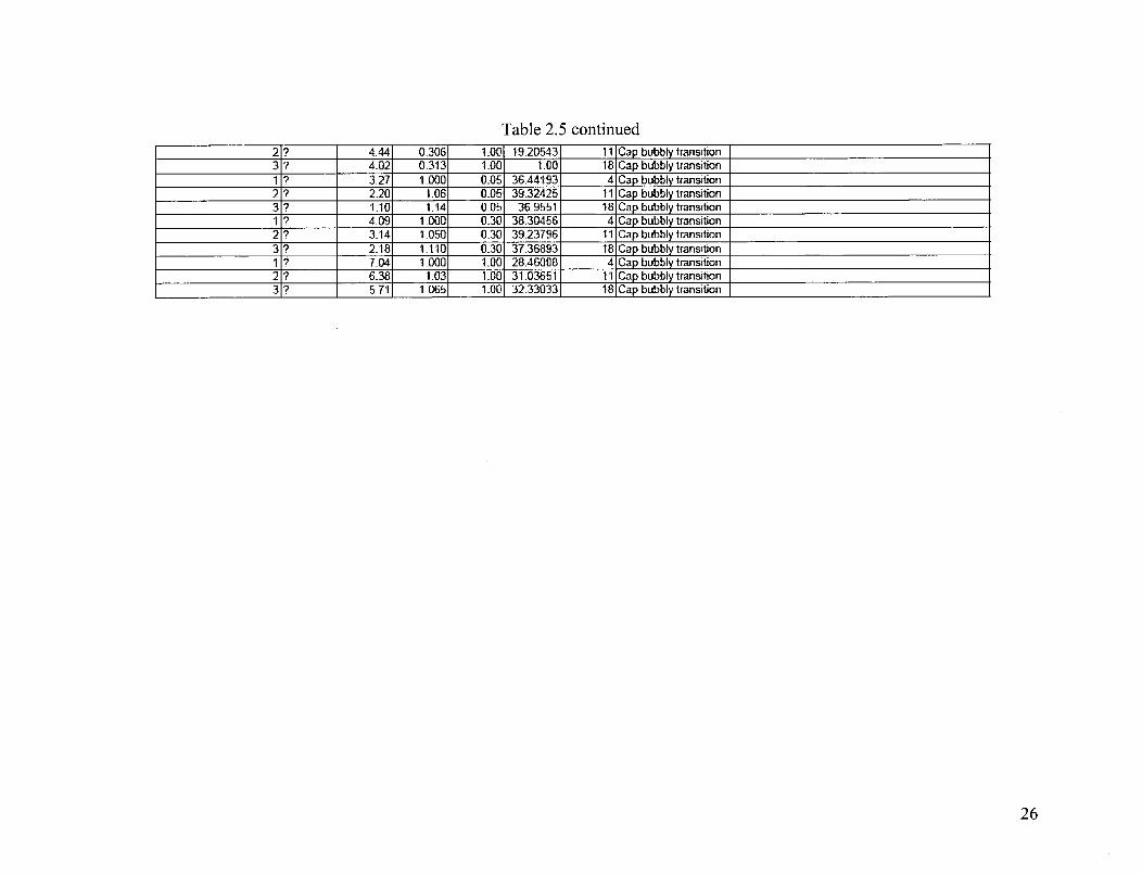
Table 2.5 continued2 ? 4.44 0.306 1.00 19.20543 11 Cap bubbly transition3 ? 4.02 0.313 1.00 1.00 18 Cap bubbly transition1 ? 3.27 1.000 0.05 36.44193 4 Cap bubbly transition2 ? 2.20 106 0.05 39.32425 11 Cap bubbly transition3 ? 1.10 1.14 0.05 36.9551 18 Cap bubbly transition1 ? 4.09 1.000 0.30 38.30456 4 Cap bubbly transition2 ? 3.14 1.050 0.30 39.23796 11 Cap bubbly transition3 ? 2.18 .110 0.30 37.36893 18 Cap bubbly transitionI ? 7.04 1.000 1.00 28.46008 4 Cap bubbly transition2 ? 6.38 1.03 1.00 31.03651 11 Cap bubbly transition3 ? 5.71 1.065 1.00 32.33033 18 Cap bubbly transition
26

2.5. Hsu et al. (2000) Data
" Measurement of void fraction using Differential Pressure Sensors.
" Pressure drop is calculated by neglecting frictional and accelerational pressure
drop, assuming hyrostatic pressure drop is dominating.
" Total 5 pressure taps are provided over the lenth of 497cm.
" Sparger Design: The gas is injected into the riser through nozzles which are made
of stainless steel tubes, having a nominal 0.015cm ID and 0.03cm OD. There are
625 such nozzles molded into an epoxy plate which is held by a plenum at the
bottom of the riser.
Eh5=481.3cm
h4=387.7cm
Test Section
h3=233cm
[ h2=93.7cm
S hl=15.8cm
Wter nlet- Air
Figure 2.5 Schematic of the test section (Hsu et al., 2000).
27

Table 2.6: Hsu et al. (2000) Data in Tabulated FormatTitleAuthorYearSource
Fluid System
Experimental study on two phase natural circulation and flow termination in a loopJ. T. Hsu, M. Ishii and T. Hibiki
2000Technical Report, Purdue University, School of Nuclear Engineering, PUfNE-00-1 1
N2-water
Test Section GeometryDiameterLengthInjector specs
10.2cm5.5m625 Nozzles: 0.015cm ID, 0.03cm OD
MeasurementMeasured parameters Inlet N2 and Water flow rate, Pressure DropInstruments Void Fraction by OPMeasurement location Three ports as indicated in the following table
Sr. No. I P J9 Jt <alpha> LJDh Flow regime Comments12 3.308 3.890 0.067 12.800 b3 3.611 3.890 0.076 26.600 b4 4.018 3.890 0.091 41.800 b5 3.264 7.780 0.058 12.800 b6 3.560 7.780 0.073 26.600 b7 3.958 7.780 0.077 41.800 b8 3.171 19.839 0.036 12.800 b9 3.456 19.839 0.046 26.600 b
10 3.841 19.839 0.050 41.800 b11 6.599 3.890 0.115 12.800 b12 7.165 3.890 0.128 26.600 bs13 7.913 3.890 0.141 41.800 s14 6.514 7.780 0.102 12.800 b15 7.072 7.780 0.113 26.600 bs16 7.817 7.780 0.127 41.800 S17 6.329 19.450 0.068 12.800 bs18 6.876 19.450 0.082 26.600 s19 7.607 19.450 0.091 41.800 S20 10.008 3.890 0.157 12.800 bs21 10.828 3.890 0.174 26.600 S22 11.910 3.890 0.166 41.800 S
28
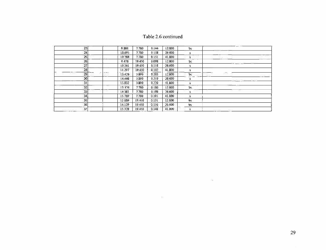
Table 2.6 continued
23 9.881 7.780 0.144- 12.800 bs24 10.695 7.780 0.158 26.600 s25 10.288 7.780 0.151 41.800 s26 9.476 19.450 0.098 12.800 bs27 10.261 19.450 0.11S 26.600 s28 11.297 19.450 0102 41.800 s29 13.426 3.890 0203 12.800 bs30 14.468 3.890 0.219 26.600 s31 15.832 3.890 0,220 41.800 s32 13-326 7.780 0.180 12.800 bs33 14.381 7.780 0.198 26.600 s34 15.769 7.780 0.195 41.800 s35 12.889 19.450 0.131 12.800 bs36 14.129 19.450 0150 26.600 bs37 15.328 19.450 0.148 41.800 s
29

2.6. Inoue Data (2001)
" Air is injected from the bottom of the vertical test section through a mixing unit.
Details of the unit is unavailable
" Local void fraction measurements are taken by an optical probe in the radial direction
and area-averaged through the cross sectional area
" Pressure correction is used while calculating the superficial gas velocity for each
probe location
Figure 2.6 Schematic of the test section (Inoue, 2001 )
30

Table 2.7: Inoue (2001) Data in Tabulated Format
Title Measurement of interfacial area concentration of gas-liquid two-phase flow in a large diameter pipeAuthor Y. lnoueYear 2001Source MS Thesis, Graduate School of Energy Science, Kyoto University, Japan
two-phase flow in a large diameter pipeFluid System Air-Water
Test Section Geometry TubeDiameter 0-2Length 25.632Injector specs Not clear, looks like perforated plate
MeasurementMeasured parameters Local parametersInstruments optical probeMeasurement location z/Dh=41.5, 82.3, 113Sr No
I P-psigl ]a if <alpha> L/Dh low regime CommentsIr - atm 0.0134 0. .13_ 41.5 NIA2 ? 0.0167 0.035 0121 41.5 NfA3 ? 0.0202 0.035 0.124 41.5 NTA4 ? 0.0235 0.035 0.109 41.5 N/A5 ? 0.0034 0.035 0.131 41.5 NIA6 ? 0.0065 0.035 0.148 41.5 NfA7 ? 0.0468 0.035 0.224 41.5 N/A8 ? 0.0736 0.035 0.227 41.5 N!A9 ? 0.1015 0.035 0.266 41.5 NIA
10 ? 0.1278 0.035 0.295 41.5 N/A
11 ? 0.1536 0.035 0.286 41.5 NIA12 ? 0.0032 0.274 0.146 41.5 NWA13 ? 0.0063 0.274 0.141 41.5 N/A14 ? 0.0097 0.274 0.143 41.5 N/A15 ? 0.0162 0.274 0.134 41.5 NWA16 ? 0.0228 0.274 0.054 41.5 NIA17 ? 0.0206 0.274 0.13 41.5 N/A18 ? 0.0418 0.274 0.024 41.5 NWA19 ? 0.0663 0.274 0.154 4,1.5 N/A20 ? 0.0932 0.274 0.119 41.5 NIA21 ? 0.1463 0.274 0.162 41.5 N/A22 ? 0.0033 0.135 0.148 41.5 N/A23 ? 0.0099 0.135 0.139 41.5 N/A24 ? 0.0162 0.135 0.277 41.5 N/A25 ? 0.0231 0.135 0.131 41.5 N/A
31

Table 2.7 continued26 ? 0.0208 0.135 0.099 41.5 N/A27 ? 0.0442 0.135 0.171 41.5 N/A28 ? 00657 0.135 013 41.5 N/A29 ? 0.0185 0-035 0-036 82.8 N/A30 ? 0.0232 0.035 0.046 82.8 N/A31 ? 0.0281 0.035 0_055 82.8 N/A32 ? 0.0329 0.035 0.066 82.8 N/A33 ? 0.0047 0.035 0.044 82.8 N/A34 ? 0.0089 0.035 0.016 82.8 N/A35 ? 0.0696 0.035 0.224 82.8 N!A36 ? 0.1124 0.035 0.291 82.8 N/A37? (0.158 0.035 0.324 82.8 N/A38? 0.1995 0.035 0.364 82.8 N/A39 ? 0.2405 0.035 0.299 82.8 N/A40 ? 0.0044 0.274 0.004 82.8 N/A41 ? 0.0086 0.274 0.004 82.8 N/A42? 0.0133 0.274 0.013 828 N/A43 ? 0.0223 0.274 0.022 82.8 N/A44 ? 0.0315 0.274 0.035 82.8 N/A45 ? 0.0288 0.274 0.064 82.8 N/A46 ? 0.0591 0.274 0.097 82.8 N/A47 ? 0.0962 0.274 0.168 82.8 N/A48 ? 0.1388 0.274 0.224 82.8 N/A49 ? 0.2232 0.274 0.29 82.8 N/A50 ? 0.0045 0.135 0.003 82.8 N/A51 ? 0.0136 0.135 0.015 82.8 NIA52? 0.0224 0.135 0.027 82.8 N/A53 ? 0.032 0.135 0.04 82.8 N/A54 ? 0.0293 0.135 0.075 82.8 N/A55 ? 0.0637 0.135 0.147 82.8 N/A56 ? 0.0953 0.135 0.172 82.8 N/A57 ? 0.0257 0.035 0.164 113 N/A58 ? 0.0323 0.035 0.181 113 N/A59? 0.0393 0.035 0.195 113 N/A60 ? 0.0461 0.035 0.208 113 N/A61 ? 0.0065 0.035 0.208 113 NIA62 ? 0.0122 0.035 0.121 113 N/A63 ? 0.1072 0.035 0.392 113 N/A64 ? 0.1809 0.035 0.443 113 N/A65 ? 0.264 0.035 0.465 113 NIA66 ? 0.0335 0.035 0.416 113 N/A67 ? 0.4066 0.035 0.455 113 N/A68 ? 0.0061 0.274 0.112 1T3 N/A
32
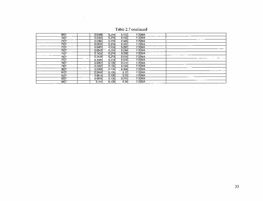
Table 2.7 continued69 ? 0.0188 0-274 0.112 113 N/A70 ? 0.0183 0-274 0.132 113 N!A71 ? 00306 0-274 0_145 113 N/A72 ? 0.0434 0.274 0_157 113 N/A73 ? 0.0403 0.274 0.207 113 N/A74 ? 0.0842 0.274 0.234 113 N/A75 ? 0.1424 0.274 0.328 113 N/A76 ? 0.2148 0.274 0.414 113 N/A77 ? 0.3595 0.274 0.424 113 N/A78 ? 0.0061 0.135 0.117 113 N/A79 ? 0.0187 0.135 0.134 113 N/A80 ? 0.0308 0.135 0.154 113 N/A81 ? 0.0444 0.135 0.17 113 N/A821? 0.0414 0.135 0.23 113 N/A831? 0.0934 0.135 0.315 113 N/A841? 0.141 0.135 0.34 1131N!A
33
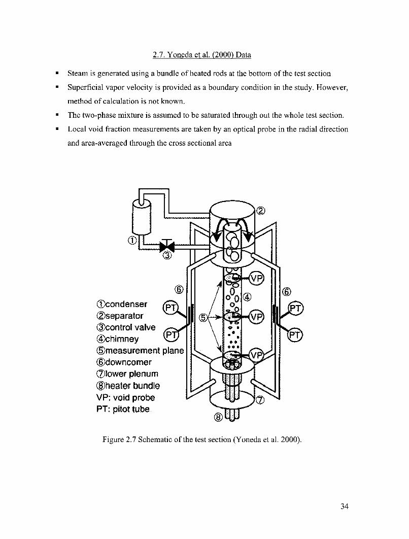
2.7. Yoneda et al. (2000) Data
" Steam is generated using a bundle of heated rods at the bottom of the test section
" Superficial vapor velocity is provided as a boundary condition in the study. However,
method of calculation is not known.
" The two-phase mixture is assumed to be saturated through out the whole test section.
" Local void fraction measurements are taken by an optical probe in the radial direction
and area-averaged through the cross sectional area
/® (4)(Dcondenser P /TZ'separator3control valve*4c hi mnneySmeasurement plane06downcomer7lower plenum
Sheater bundleVP: void probePT: pitot tube
Figure 2.7 Schematic of the test section (Yoneda et al. 2000).
34

Table 2.8: Yoneda et al. (2000) Data in Tabulated Format
Title.uthor
Y'earSource
Fluid System
Flow Structure of Developing Steam-water Two-phase Flow in Large Diameter PipeYoneda et al.
2000Proc. 8th Int. Conf. Nucl. Eng.
Steam-Water
rest Section GeometryDiameterLength
njector specs
MeasurementMleasured parametersnstrumentsMeasurement location
Tube0.1552
0.7 approximatelyno injector
Local parametersoptical probeziDh=0.48, 2.42,4.35
Sr. No. T P(kPa) f <alpha> 1Dh Flow regime Comments1 151.8 500.00 0.25 0.59 0.324812 2.42 N/A 1y given by the author, T is assumed to be sat temp2 151.8 500.00 02 0.55 0.271115 2.42 N/A yg given by the author, T is assumed to be sat temp3 151.8 500.00 0.15 0.5 0.221123 2.42 NIA jg given by the author, T is assumed to be sat temp4 151.8 500.00 0.1 0.43 0.166239 2.42 NIA jg given by the author, T is assumed to be sat temp5 151.8 500.00 0.05 0.34 0.104982 2.42 N/A Ig given by the author, T is assumed to be sat temp6 151.8 500.00 0.01 0.21 0..037813 2.42 NIA !g given by the author, T is assumed to be sat temp7 151.8 500.00 0.25 0.59 0.346152 4.35 NIA jg given by the author, T is assumed to be sat temp8 151.8 500.00 0.2 0.55 0.288403 4.35 NIA jg given by the author, T is assumed to be sat temp9 151.8 500.00 0.15 0.5 0.233003 4.35 N/A jg given by the author, T is assumed to be sat temp
10 151.8 500.00 0.1 0.43 0.174679 4.35 N/A jg given by the author, T is assumed to be sat temp11 151.8 500.00 0.05 0.34 0.113729 4.35 N/A !9 given by the author, T is assumed to be sat temp12 151.8 500.00 0.01 0.21 0.041891 4.35 NIA jg given by the author, T is assumed to be sat temp
35

CHAPTER 3 CORRELATIONS AND PRELIMINARY COMPARISONS
Important correlations based on drift flux model for the prediction of void fraction
in a large diameter pipe are considered. The correlations typically express the
distribution parameter Co and the drift velocity ((vg)) as a function of fluid properties,
flow geometry and void fraction (in some cases). Hence void fraction can be calculated
implicitly using the boundary conditions, i.e. superficial gas and liquid velocities. A
preliminary comparison of the void fraction correlations with the experimental data by
Hills (1976) is presented. The calculated void fraction is plotted against measured data
with error lines showing error of ±20%.
3.1 Drift Flux Model by Hills(1976)
Hills (1976) measured void fraction in an air-water bubble colunm with an inner
diameter of 0.150 m and height of 10.5 m at gas superficial velocities of 0.070 - 3.5 m/s
and liquid superficial velocities of 0 - 2.7 m/s. Hills developed the following drift-flux
type correlations based on his own data base.
((Vg)) = 1.35(j)93 + 0.24, for (jf) > 0.3 m/s, (3-1)
(Jg) (Jf) -0.24 +4.0(01.72, for (jf<0.3m/s (3-2)(a) 1- (a)
where jf is the superficial liquid velocity. In these correlations, the unit of
parameters should be m/s. Since the mixture volumetric flux in his experiment should be
6.2 rn/s at maximum, Eqs.(3-1) and (3-2) can be recast as Eqs.(3-3) and (3-4),
respectively.
((vg)) = 1.2(j) + 0.24, for (j!) > 0.3 m/s, (3-3)
36

((Vg)):(j)+(4.0(a)'72 +0.24l- (a)), for (jf)_• 0.3 m/s. (3-4)
It should be noted here that Hills did not consider the effect of physical properties
on the distribution parameter and the drift velocity in his correlation. Figure 3-1 shows
the comparison of void fraction predicion by Hills (1976) correlation with Hills (1976)
data.
0.9
0.8
0.7
00.6
LL
~00.5
E 0.40
0.3
0.2
0.1
1Measured Void Fraction
Figure 3.1 Comparison of void fraction predicion by Hills (1976) correlation with Hills
(1976) data.
3.2 Drift flux model by Shiplev (1984)
Shipley (1984) measured void fraction of air-water bubbly flow in a pipe with an
inner diameter of 0.457 m and height of 5.64 m. Shipley proposed the following
correlation based on his own data base.
37

(vg ))=1.2Cb+{0.24+ 0.35 j D(a) (3-5)
In this correlation, the unit of parameters should be m/s. It should be noted here
that the second term in the right hand side of this correlation corresponding to the drift
velocity can become very large for a very large diameter pipe, which may give
unphysical results. Figure 3-2 shows the comparison of void fraction predicion by
Shipley (1984) correlation with Hills (1976) data.
1 1
0.9 -
0.8 -
0.7 -
0" 0.6 -
LjL-0
, 0.5
E 0.4-8
0.3-
0.2 -
0.1
S0 0.1 0.2 0.3 0.4 0.5 0.6 0.7 0.8 0.9 1Measured Void Fraction
Figure 3.2 Comparison of void fraction predicion by Shipley (1984) correlation with Hills
(1976) data.
3.3 Drift flux model bv Clark and Flemmer (1985)
Clark and Flemmer (1985) measured void fraction of air-water bubbly flow in a
pipe with an inner diameter of 0.10 m. Mixture volumetric fluxes and void fractions
38
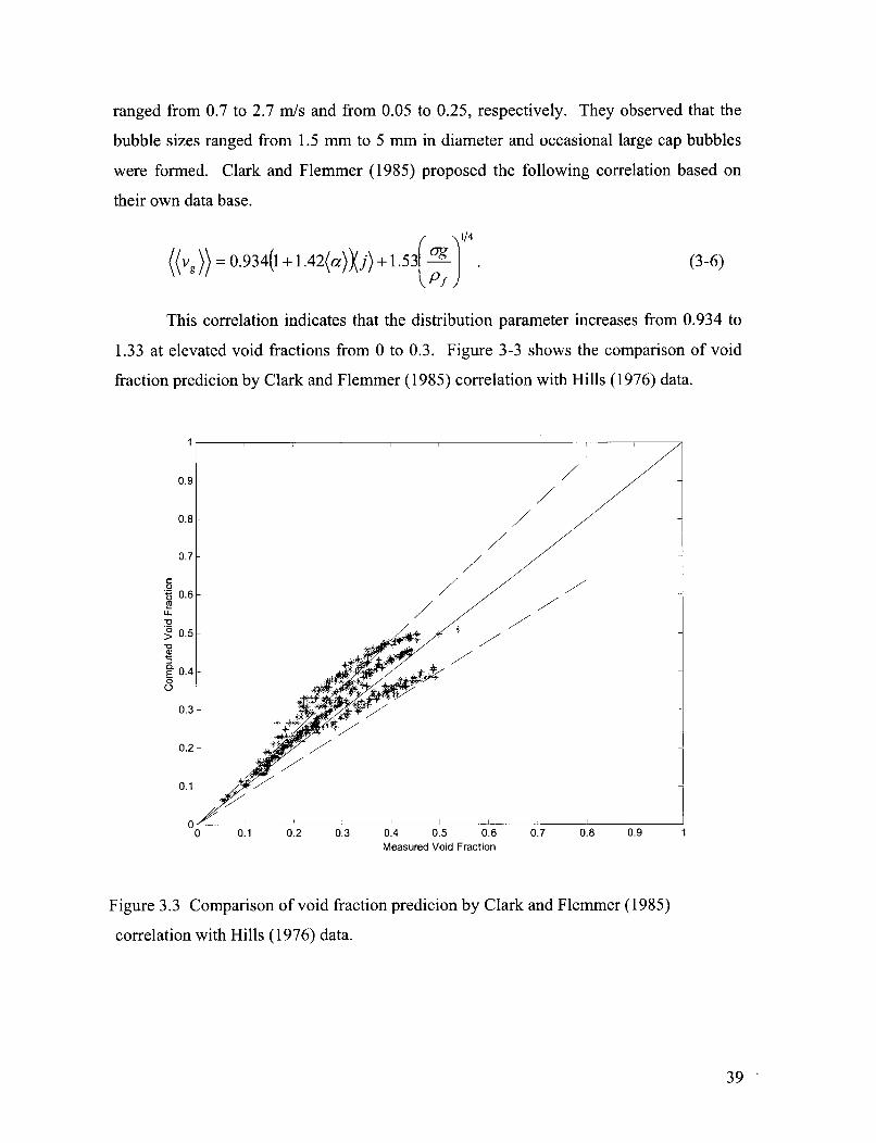
ranged from 0.7 to 2.7 m/s and from 0.05 to 0.25, respectively. They observed that the
bubble sizes ranged from 1.5 mm to 5 mm in diameter and occasional large cap bubbles
were formed. Clark and Flemmer (1985) proposed the following correlation based on
their own data base.
((v,)) = 0.934(1±1.42(aý)j) + 1.53 j/ (3-6)
This correlation indicates that the distribution parameter increases from 0.934 to
1.33 at elevated void fractions from 0 to 0.3. Figure 3-3 shows the comparison of void
fraction predicion by Clark and Flemmer (1985) correlation with Hills (1976) data.
0.9 -
0.8-
0.7
0" 0.6
IL
*0> 0.5-
E. 0.4-
0.3
0.1
0 0.1 0.2 0.3 0.4 0.5 0.6 0.7 0.8 0.9 1Measured Void Fraction
Figure 3.3 Comparison of void fraction predicion by Clark and Flemmer (1985)
correlation with Hills (1976) data.
39

3.4 Drift flux model by Kataoka and Ishii (1987)
Kataoka and Ishii (1987) found that the drift-velocity in a pool system depended
upon vessel diameter, system pressure, gas flux and fluid physical properties, and
developed the following correlation for the pool void fraction based on extensive data
bases taken under various experimental conditions.
Low viscous case: Ngf_< 2.25 x 10⁻³
/--f/-0.157,Vg= 0.0019DH*/°8°9 p-5 ,v°'62, for DM < 30,
S . -0 .1 5 7 - -
Vg• = 0.03OLj0.030 N-° 62 ,for D, >Ž30,
Higher viscous case: Ngf> 2.25 x 10⁻³
(3-7)
(3-8)
V9+ = 0. 9 2 0.157
gi ~Pj, for D,*>_30, (3-9)
where Vgj+ and Nvf are the non-dimensional drift velocity and the viscous number,
respectively, defined as
and N. : 1/2•
LPfU U
(3-10)
For a fully developed turbulent flow in a round tube,
CO = 1.2 -0.2Pg/pj. (3-11)
Figure 3-4 shows the comparison of void fraction predicion by Kataoka and Ishii (1987)
correlation with Hills (1976) data.
40

0.4 0.5 0.6Measured Void Fraction
Figure 3.4 Comparison of void fraction predicion by Kataoka and Ishii (1987) correlation
with Hills (1976) data.
3.5 Drift flux model by Ishii and Kocamustafaogullari (1985)
Ishii and Kocamustafaogullari (1985) developed a theoretical correlation of the
drift velocity for cap bubble flow inside a large diameter channel. It is given by
Vg1 = 0.54 , forDh 30 (3-12)Pf
{-"1/4
V.s = 3.0 [ for D* > 30 (3-13)gjpr 2 I
41

where Dh is the hydraulic diameter. The non-dimensional hydraulic diameter, D*
is defined by
*= DhDh = (3-14)fo"/ gap'
Figure 3-5 shows the comparison of void fraction predicion by Ishii and
Kocamustafaogullari (1985) correlation with Hills (1976) data.
0.97
0.8 -/
0.7-/
0"- 0.6-
IL
E .- +-0.3
0.2 -
0.1
_ _f1I III
0 0.1 0.2 0.3 0.4 0.5 0.6 0.7 0.8 0.9Measured Void Fraction
Figure 3.5 Comparison of void fraction predicion by Ishii and Kocamustafaogullari
(1985) correlation with Hills (1976) data.
42

3.6 Drift Flux Model by Hibiki and Ishii (2003)
Hibiki and Ishii (2003) reviewed existing analytical and experimental studies
related to two-phase flow in a large diameter pipe. The following table shows the
recommended drift flux correlations.
Table 3.1: Drift-flux correlations recommended by Hibiki and Ishii (2003).
Flow Regime Recommended Drift-Flux Correlation
Bubbly or Cap Bubbly Flow + Fo , forCO = exp .4751
<a> <ý 0.3 P ,
Inlet Flow Regime : °-(Ji,)/(J+) •0.9,
Uniformly-Distributed r ri/ } forBubbly Flow C.= -2.88LNk)J +±4.0811- +
0.9 4<-(j;)/(j+) < I"
V. = V.,, exp(-1.39(jg))+ V exp(- 1.39(]j))}.
Cap Bubbly Flow 1. 1 (j_)2.22 1 , forCO = \/IC .2expI 0!\II
<a>•< 0.3 P0-• (j+)- 1.8s,
Inlet Flow Regime:
Cap Bubbly or Slug Flow Co = [0.6cxp{-1.2((j-)-1.8)}+1.2Q- - for 1.8
g = P;,P *
Cap Bubbly Flow cO = 1.2- 0.2 pg/p•
<a> >0.3 Low viscous case: N f< 2.25 x 10⁻³
ýE f '-0 .157 o r D :ý
V÷ = 0.0019D;,o.809 -0.56 2 , for DH 30,ii P N) -
+= 0.030 N 0562 for D, > 30,
PfHigher viscous case: Nf > 2.25 x 10⁻³
(. .- 015 7
VI = 0.92 - ,for D, _>30.gi Ci
43

Flow Regime
Chum Flow
Table 3.1 continued
Recommended Drift-Flux Correlation
Co = 1.2-0.2Pg/pf,
S 1/4
Annular Flow
Vgj =Vgj+(C0-1X).
44

CHAPTER 4 SUMMARY
Extensive literature survey of the available void fraction correlations for two-phase
flow in large diameter pipes is carried out. The database available in the literature is
assembled in numerical form. The database involves specifications of boundary
conditions, fluid properties and measured volume or area averaged void fraction.
However, it should be noted that the thermodynamic state of the fluids was not clearly
provided in all the data sets. Hence, certain assumptions on the fluid properties have to
be made in the evaluation of the data. Also, the local superficial gas and liquid velocities
were not clearly specified due to the lack of data on local pressure at the measurement
location in some cases. Furthermore, the available data does no include flow conditions
at higher void fraction (a > 0.6) and in chum-turbulent to annular flow transition. The
available correlations are based on drift flux model, in which the distribution parameter
and the drift velocity are specified through empirical correlations. Simple computer code
is written for the evaluation of these available correlations and for the comparison of the
predicted void fraction with the available data. Preliminary comparisons of the void
fraction correlations are made.
45

REFERENCES
Clark N. N. and Flemmer R. L., 1985. Predicting the holdup in two-phase bubble upflowand downflow using the Zuber and Findlay drift-flux model. AIChE Journal, 31, pp. 500-503.
Hall, W.H., Prueter, W.P., Thome, T.L., and Wall, J.R. 1988. High-pressure steam/watervoid fraction profiles in a large-diameter, vertical pipe with non-developed entrance flow,Thermal Hydraulics of Nuclear Steam Generators/Heat Exchangers, Nov 27-Dec 2 1988,Chicago, IL, USA, pp. 53-60.
Hashemi, A., Kim, J. H. and Sursock, J. P. 1986. Effect of diameter and geometry ontwo-phase flow regimes and carry-over in a model PWR hot leg, Proceedings of 8 th
International Heat Transfer Conference, San Francisco, CA, USA, pp.2443-2451.
Hibiki, T. and Ishii, M., 2003. One-dimensional drift flux model for two-phase flow in alarge diameter pipe. International Journal of Heat and Mass Transfer, 46, pp. 1773-1790.
Hills, J. H., 1976. The Operation of a bubble column at high throughputs I. Gas holdupMeasurements. The Chemical Engineering Journal, 12, pp. 89-99.
Hsu, J.T., Ishii, M., and Hibiki, T., 1988. Experimental study on two-phase naturalcirculation and flow termination in a loop, Nucl. Eng. Des., 186, pp. 395-409.
Inoue, Y. 2001. Measurement of interfacial area concentration of gas-liquid two-phaseflow in a large diameter pipe, MS Thesis, Graduate School of Energy Science, KyotoUniversity, Japan, 2001.
Ishii M. and Kocamustafaogullari G., Private communication (1984). Also Maximumfluid particle size for bubbles and drops, Proceedings of ASME Winter Annual Meeting,Miami Beach, FL, USA, FED-vol.29, 1985, pp. 9 9 - 10 7 .
Kataoka I. and Ishii M., 1987. Drift flux model for large diameter pipe and newcorrelation for pool void fraction. International Journal of Heat and Mass Transfer, 30,pp. 1927-1939.
Shipley, D. G, 1984. Two phase flow in large diameter pipes. Chemical EngineeringScience, 39, pp. 163-165.
T. R. Smith, 2002, Two-group Interfacial Area Transport Equation in Large DiameterPipes, PhD Thesis, Purdue University, West Lafayette, USA.
46
Yoneda, K., Yasuo, A., Okawa, T. and Zhou S. R. 2000. Flow structure of developingsteam-water two-phase flow in a large-diameter pipe, Proceedings of 8th InternationalConference on Nuclear Engineering, Baltimore, MD, USA.
47
APPENDIX
The database from literature is organized in Excell worksheets. This worksheet
contains the values of superficial gas and liquid velocities and the measured void fraction
for each observation. Fluid properties data is also included in the Excell worksheet. In
addition, a flow regime indicator is specified for each flow condition. The flow regimes
are specified as follows:
1. Bubbly Flow
2. Cap-Bubbly Flow
3. Slug Flow
4. Chum-Turbulent Flow
5. Annular Flow.
The worksheets are named after the first author. All the worksheets are
assembled in a single Excell file named: largedata.xls. An example excell worksheet is
shown in Table A-1. A MatLab script is written for calculation of void fraction and
comparison with data. The main script file (named: mainlarg.m) takes the above
mentioned Excell file as input. The name of the worksheet is specified in the script file.
Separate function scripts are written for each correlation. These functions are called by
the main script to evaluate the void fraction from the superficial gas and liquid velocity
data. Further, the main script saves the calculated void fraction data in an output file.
Also, a plot of calculated void fraction vs. the measured void fraction is generated by the
program. The listing of the main script as well as the functions is provided in this
appendix.
48
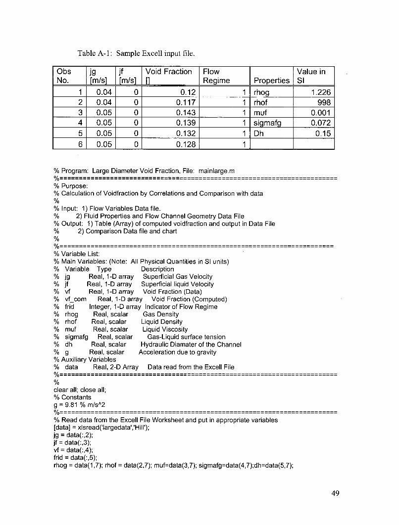
Table A- 1: Sample Excell input file.
Obs [g jf Void Fraction Flow Value inNo. [m/s] [ms [M/] Regime Properties Sl
1 0.04 0 0.12 1 rhog 1.2262 0.04 0 0.117 1 rhof 9983 0.05 0 0.143 1 muf 0.0014 0.05 0 0.139 1 sigmafg 0.0725 0.05 0 0.132 1 Dh 0.156 0.05 0 0.128 1
% Program: Large Diameter Void Fraction, File: mainlarge.m
% Purpose:% Calculation of Voidfraction by Correlations and Comparison with data
% Input: 1) Flow Variables Data file.% 2) Fluid Properties and Flow Channel Geometry Data File% Output: 1) Table (Array) of computed voidfraction and output in Data File* 2) Comparison Data file and chart
% Variable List:% Main Variables: (Note: All Physical Quantities in SI units)% Variable Type Description% jg Real, 1-D array Superficial Gas Velocity% jf Real, 1-D array Superficial liquid Velocity% vf Real, 1-D array Void Fraction (Data)% vfcom Real, 1-D array Void Fraction (Computed)% frid Integer, 1-D array Indicator of Flow Regime% rhog Real, scalar Gas Density% rhof Real, scalar Liquid Density% muf Real, scalar Liquid Viscosity% sigmafg Real, scalar Gas-Liquid surface tension% dh Real, scalar Hydraulic Diamater of the Channel% g Real, scalar Acceleration due to gravity% Auxiliary Variables% data Real, 2-D Array Data read from the Excell File
clear all; close all;% Constantsg = 9.81 % m/s^2
% Read data from the Excell File Worksheet and put in appropriate variables[data] = xlsread('largedata','Hill');jg = data(:,2);jf = data(:,3);vf = data(:,4);frid = data(:,5);rhog = data(1,7); rhof = data(2,7); muf=data(3,7); sigmafg=data(4,7);dh=data(5,7);
49
[ndata,col] = size(data);clear data;
% Execute the suboutine to compute void fraction from correlation[vfcom] = compute voidkojasoy(ndata,jg,jf,frid,rhog,rhof,muf,sigmafg,dh,g);
% Save data in a textfilefoutid = fopen('largeoutKojasoyHill.txt','w');fprintf(foutid,'%5s \t %5s \t %5s \t %6s \n','jg','jf`,'vf,'vf_com');fprintf(foutid,'%5.3f \t %5.3f \t %5.3f \t %5.3f \n',ig';jf;vf;vf_com]);fclose(foutid);% Plot graphdum = [0,1];plot(vf,vf com,'*',du m,dum,'k-');hold on;dum = [0,0.8]; duml=[0,0.8*1.2];dum2=[0,0.8*0.8];plot(dum,duml ,'k--',dum,dum2,'k--')axis([0,1,0,1]); xlabel('Measured Void Fraction'); ylabel('Computed Void Fraction')% End of Program
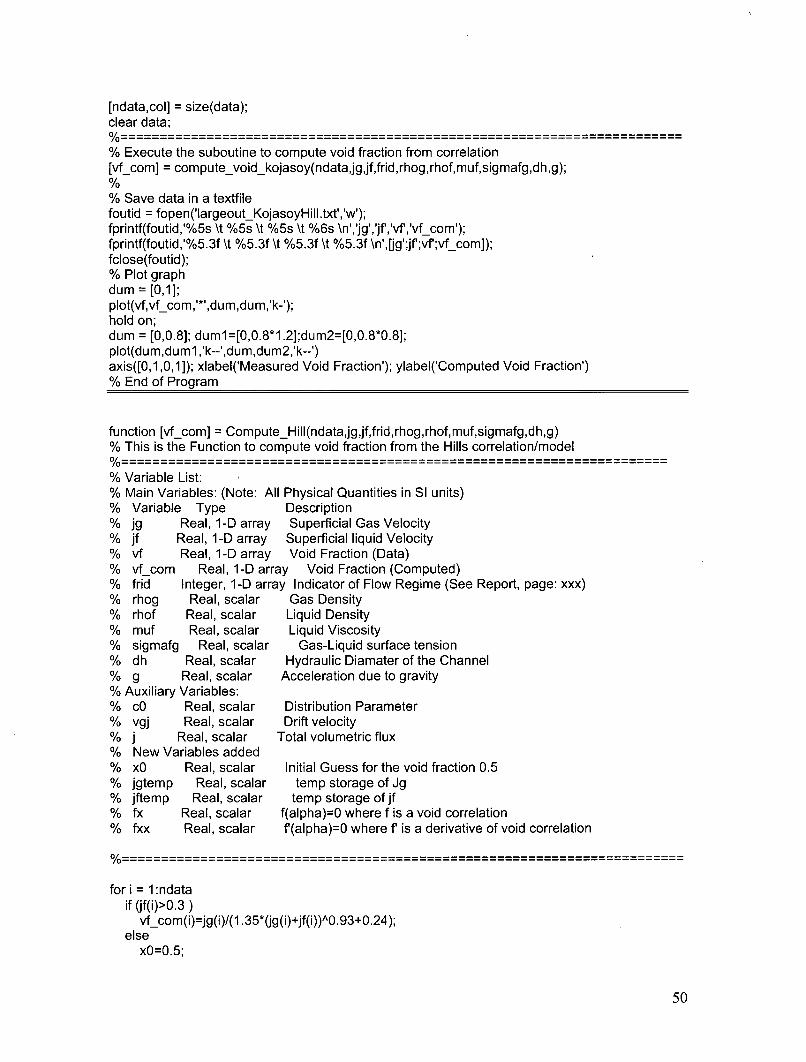
function [vf com] = Compute_Hill(ndata,jg,jf,frid,rhog,rhof, muf,sigmafg,dh,g)% This is the Function to compute void fraction from the Hills correlation/model
% Variable List:% Main Variables: (Note: All Physical Quantities in SI units)% Variable Type Description% jg Real, 1-D array Superficial Gas Velocity% jf Real, 1-D array Superficial liquid Velocity% vf Real, 1-D array Void Fraction (Data)% vfcom Real, 1-D array Void Fraction (Computed)% frid Integer, 1-D array Indicator of Flow Regime (See Report, page: xxx)o%%0 rhog Real, scalar
rhof Real, scalarmuf Real, scalarsigmafg Real, scalardh Real, scalarg Real, scalar
Auxiliary Variables:cO Real, scalarvgj Real, scalarj Real, scalarNew Variables addedx0 Real, scalarjgtemp Real, scalarjftemp Real, scalarfx Real, scalarfxx Real, scalar
Gas DensityLiquid DensityLiquid Viscosity
Gas-Liquid surface tensionHydraulic Diamater of the Channel
Acceleration due to gravity
Distribution ParameterDrift velocity
Total volumetric flux
Initial Guess for the void fraction 0.5temp storage of Jgtemp storage of jf
f(alpha)=0 where f is a void correlationf(alpha)=0 where f' is a derivative of void correlation
for i = 1 :ndataif (jf(i)>0.3)
vfcom(i)=jg(i)/(1.35*(jg(i)+jf(i))A0.93+0.24);else
x0=0.5;
50

jgtemp=jg(i);jftemp=jf(i);
for j=1:10000[fx]=Hill_l (jgtemp,jftemp,xO);if (abs(fx)<=0.0001)
break;else
[fxx]=Hill_2(jgtemp,jftemp,x0);ximp=x0-fx/fxx;x0=ximp;
endend
vf com(i)=xO;end
end% End of Function
function [fx] = Hill_l(jgtemp,jftemp,x)fx=0.24+4.0*(x)A^ .72-jgtemp/x+jftemp/(1 -x);
function [fxx] = Hill_2(jgtemp,jftemp,x)fxx=4.0*1.72* (x)A .72+jgtemp/(xA2)+jftemp/(1 -x)A 2;
function [vfcom] = ComputeShipley(ndata,jg,jf,frid,rhog,rhof,muf,sigmafg,dh,g)% This is the Function to compute void fraction from the Shipley correlation/model
% Variable List:% Main Variables: (Note: All Physical Quantities in SI units)% Variable Type Description% jg Real, 1-D array Superficial Gas Velocity% jf Real, 1-D array Superficial liquid Velocity% vf Real, 1-D array Void Fraction (Data)% vfcom Real, 1-D array Void Fraction (Computed)% frid Integer, 1-D array Indicator of Flow Regime (See Report, page: xxx)% rhog Real, scalar Gas Density% rhof Real, scalar Liquid Density% muf Real, scalar Liquid Viscosity% sigmafg Real, scalar Gas-Liquid surface tension% dh Real, scalar Hydraulic Diamater of the Channel% g Real, scalar Acceleration due to gravity% Auxiliary Variables:% cO Real, scalar Distribution Parameter% vgj Real, scalar Drift velocity% j Real, scalar Total volumetric flux% New Variables added% x0 Real, scalar Initial Guess for the void fraction 0.5% jgtemp Real, scalar temp storage of Jg% jftemp Real, scalar temp storage of jf% fx Real, scalar f(alpha)=0 where f is a void correlation% fxx Real, scalar f'(alpha)=0 where f' is a derivative of void correlation
51
for i = l:ndatax0=0.5;jgtemp=jg(i);jftemp=jf(i);
for j= 1:10000[fx]=Shipleyl (jgtemp,jftemp,xO,dh,g);if (abs(fx)<=0.0001)
break;else
[fxx]=Shipley_2(jgtemp,jftemp,xO,dh,g);ximp=x0-fx/fxx;xO=ximp;
endend
vf com(i)=xO;
end% End of Function
function [fx] = Shipley_l(jgtemp,jftemp,x,dh,g)fx=1.2*(gtemp+jftemp)*x+x*(0.24+0.35*( gtemp/ gtemp+jftemp))A2)*sqrt(g*dh*x))-jgtemp;
function [fxx] = Shipley_2(jgtemp,jftemp,x,dh,g)fxx=1.2*(jgtemp+jftemp)+0.24+1.5*0.35*((jgtemp/(jgtemp+jftemp))A2)*sqrt(g*dh*x);
function [vfcom] = Compute clrkflm(ndata,jg,jf,frid,rhog,rhof,muf,sigmafg,dh,g)% This is the Function to compute void fraction from the Clark-Flemmer Model% Newton-Raphson Mehtod used to solve the non-linear equation
% Variable List:% Main Variables: (Note: All Physical Quantities in SI units)% Variable Type Description% jg Real, 1-D array Superficial Gas Velocity% jf Real, 1-D array Superficial liquid Velocity% vf Real, 1-D array Void Fraction (Data)% vfcorn Real, 1-D array Void Fraction (Computed)% frid Integer, 1-D array Indicator of Flow Regime (See Report, page: xxx)% rhog Real, scalar Gas Density% rhof Real, scalar Liquid Density% muf Real, scalar Liquid Viscosity% sigmafg Real, scalar Gas-Liquid surface tension% dh Real, scalar Hydraulic Diamater of the Channel% g Real, scalar Acceleration due to gravity% Auxiliary Variables:% cO Real, scalar Distribution Parameter% vgj Real, scalar Drift velocity% j Real, scalar Total volumetric flux
% New Variables added% x0 Real, scalar Initial Guess for the void fraction 0.5% jgtemp Real, scalar temp storage of Jg% jftemp Real, scalar temp storage of jf% fx Real, scalar f(alpha)=0 where f is a void correlation
52
% fxx Real, scalar f'(alpha)=0 where f is a derivative of void correlation
for i = 1:ndatax0=0.5;jgtemp=jg(i);jftemp=jf(i);
for j=1:10000000[fx]=clrkflml (jgtemp,jftemp,xO,sigmafg,rhof,g);if (abs(fx)<=0.0001)
break;else
[fxx]=clrkflm_2(jgtemp,jftemp,x0,sigmafg,rhof,g);ximp=xO-fx/fxx;x0=ximp;
endend
vf-com(i)=x0;
end% End of Function
function [fx] = clrkflm_l(jgtemp,jftemp,x,sigmafg,rhof,g)fx=0.934*x*(1 +1.42*x)*(jgtemp+jftemp)+ 1.53*x*(sigmafg*g/rhof)A0.25-jgtemp;
function [fxx] = clrkflm_2(jgtemp,jftemp,x,sigmafg,rhof,g)fxx=(0.934+(2.0*1.42*0.934*x))*(jgtemp+jftemp)+1.53*(sigmafg*g/rhof)A0.25;
function [vf com] = computeKataoka void(ndata,jg,jf,frid,rhog,rhof,muf,sigmafg,dh,g)% This is the Function to compute void fraction from the correlation/model
% Variable List:% Main Variables: (Note: All Physical Quantities in SI units)% Variable Type Description% jg Real, 1-D array Superficial Gas Velocity% jf Real, 1-D array Superficial liquid Velocity% vf Real, 1-D array Void Fraction (Data)% vfcom Real, 1-D array Void Fraction (Computed)% frid Integer, 1-D array Indicator of Flow Regime (See Report, page: xxx)% rhog Real, scalar Gas Density% rhof Real, scalar Liquid Density% muf Real, scalar Liquid Viscosity% sigmafg Real, scalar Gas-Liquid surface tension% dh Real, scalar Hydraulic Diamater of the Channel% g Real, scalar Acceleration due to gravity% Auxiliary Variables:% cO Real, scalar Distribution Parameter% vgj Real, scalar Drift velocity% j Real, scalar Total volumetric flux
delrho = rhof-rhog;rhoratio = rhog/rhof;Ls = (sigmafg/g/delrho)AO.5;Vs = (sigmafg*g*(rhof-rhog)/rhofA2)A0.25;
53

Dhs = dh/Ls;N_muf= muf/(rhof*sigmafg*Ls)AO.5;
cO = 1.2-0.2*(rho-ratio)A0.5;
if (Nmuf <= 2.25e-3)if (Dhs <=30)
vgjp = 0.0019*DhsAO .809*rhoratioA(-0. 157)*NmufA(-0.562);else
vgjp = 0.030*rhoratioA(-0.157)*NmufA(-0.562);end
elsevgjp = 0.92*rhoratioA(-0.157);
endvgj = vgjp*Vs;
for i = 1:ndatavf com(i) = jg(i)/(cO*(jg(i)+jf(i))+vgj);
end% End of Function
function [vf com] = compute void(ndata,jg,jf,frid,rhog,rhof,muf,sigmafg,dh,g)% This is the Function to compute void fraction from the lshii&Kojasoy correlation
% Variable List:% Main Variables: (Note: All Physical Quantities in SI units)% Variable Type Description% jg Real, 1-D array Superficial Gas Velocity% jf Real, 1-D array Superficial liquid Velocity% vf Real, 1-D array Void Fraction (Data)% vfcom Real, 1-D array Void Fraction (Computed)% frid Integer, 1-D array Indicator of Flow Regime (See Report, page: xxx)% rhog Real, scalar Gas Density% rhof Real, scalar Liquid Density% muf Real, scalar Liquid Viscosity% sigmafg Real, scalar Gas-Liquid surface tension% dh Real, scalar Hydraulic Diamater of the Channel% g Real, scalar Acceleration due to gravity% Auxiliary Variables:% cO Real, scalar Distribution Parameter% vgj Real, scalar Drift velocity% j Real, scalar Total volumetric flux
delrho = rhof-rhog;rhoratio = rhog/rhof;Ls = (sigmafg/g/delrho)AO.5;Vs = (sigmafg*g*(rhof-rhog)/rhofA2)A0.25;Dhs = dh/Ls;N_muf= muf/(rhof*sigmafg*Ls)A0.5;
cO = 1.2-0.2*(rhoratio)A0.5;
if (Dhs <=30)vgj=0.54*(g*dh*delrho/rhof)A(0.5);
elsevgj=3.0*(sigmafg*g*delrho/(rhofA2))A(0 .25);
54
end
for i = 1:ndatavf com(i) = jg(i)/(cO*(jg(i)+jf(i))+vgj);
end% End of Function
55