Embed Size (px)
Citation preview

Annual report
ENVIRONMENTAL
MONITORING
M-694 | 2016
Monitoring of greenhouse gases
and aerosols at Svalbard and
Birkenes in 2015

1
COLOPHON
Executive institution
NILU – Norsk institutt for luftforskning
P.O. Box 100, 2027 Kjeller
ISBN: 978-82-425-2862-9 (electronic)
ISSN: 2464-3327
Project manager for the contractor Contact person in the Norwegian Environment Agency
Cathrine Lund Myhre Camilla Fossum Pettersen
M-no Year Pages Contract number
694 2016 125 15078041
Publisher The project is funded by
NILU – Norsk institutt for luftforskning
NILU report 31/2016
NILU project no. O-99093/O-105020/O-113007
Norwegian Environment Agency and
NILU – Norwegian Institute for Air Research.
Author(s)
C.L. Myhre, O. Hermansen, M. Fiebig, C. Lunder, A.M. Fjæraa, T. M. Svendby, S. M. Platt, G. Hansen,
N. Schmidbauer, T. Krognes
Title – Norwegian and English
Monitoring of greenhouse gases and aerosols at Svalbard and Birkenes in 2015 - Annual report
Overvåking av klimagasser og partikler på Svalbard og Birkenes i 2015: Årsrapport
Summary – sammendrag
The report summaries the activities and results of the greenhouse gas monitoring at the Zeppelin
Observatory situated on Svalbard in Arctic Norway during the period 2001-2015, and the greenhouse
gas monitoring and aerosol observations from Birkenes for 2009-2015.
Rapporten presenterer aktiviteter og måleresultater fra klimagassovervåkingen ved Zeppelin
observatoriet på Svalbard for årene 2001-2015 og klimagassmålinger og klimarelevante
partikkelmålinger fra Birkenes for 2009-2015.
4 emneord 4 subject words
Drivhusgasser, partikler, Arktis, halokarboner Greenhouse gases, aerosols, Arctic,
halocarbons
Front page photo
Ny-Ålesund, Svalbard. Photo: Kjetil Tørseth, NILU.

Monitoring of greenhouse gases and aerosols at Svalbard and Birkenes in 2015 | M-694 | 2016
1
Preface
This report presents results from the national monitoring of greenhouse gases and aerosol
properties in 2015. The observations are done at two atmospheric supersites; one regional
background site in southern Norway and one Arctic site. The observations made are part of
the national monitoring programme conducted by NILU on behalf of The Norwegian
Environment Agency.
The monitoring programme includes measurements of 41 greenhouse gases at the Zeppelin
Observatory in the Arctic; and this includes a long list of halocarbons, which are not only
greenhouse gases but also ozone depleting substances. The number of measured species has
increased by 16 since the report in 2014. In 2009, NILU upgraded and extended the
observational activity at the Birkenes Observatory in Aust-Agder and from 2010, the national
monitoring programme was extended to also include greenhouse gas observations and
selected aerosol observations particularly relevant for understanding the interactions
between aerosols and radiation.
The present report is the fourth of a series of annual reports for 2015, which cover the
national monitoring of atmospheric composition in the Norwegian rural background
environment. The other three reports are focuses on the atmospheric composition and
deposition of air pollution of particulate and gas phase of inorganic constituents, particulate
carbonaceous matter, ground level ozone and particulate matter, the second on persistent
organic pollutants and heavy metals, and the third presents the monitoring of the ozone layer
and UV.
Data and results from the national monitoring programme are also included in various
international programmes, including: EMEP (European Monitoring and Evaluation Programme)
under the CLTRAP (Convention on Long-range Transboundary Air Pollution), AGAGE (Advanced
Global Atmospheric Gases Experiment), CAMP (Comprehensive Atmospheric Monitoring
Programme) under OSPAR (the Convention for the Protection of the marine Environment of
the North-East Atlantic) and AMAP (Arctic Monitoring and Assessment Programme). Data from
this report are also contributing to European Research Infrastructure network ACTRIS
(Aerosols, Clouds, and Trace gases Research InfraStructure Network) and implementation in
ICOS (Integrated Carbon Observation System) is in progress.
All measurement data presented in the current report are public and can be received by
contacting NILU, or they can be downloaded directly from the database: http://ebas.nilu.no.
A large number of persons at NILU have contributed to the current report, including those
responsible for sampling, technical maintenance, chemical analysis and quality control and
data management. In particular Cathrine Lund Myhre (coordinating the program), Ove
Hermansen, Chris Lunder, Terje Krognes, Stephen M. Platt, Norbert Schmidbauer, Ann Mari
Fjæraa, Kerstin Stebel, Markus Fiebig, and Tove Svendby.
NILU, Kjeller, 23 November 2016
Cathrine Lund Myhre
Senior Scientist, Dep. Atmospheric and Climate Research

Monitoring of greenhouse gases and aerosols at Svalbard and Birkenes in 2015 | M-694 | 2016
2
Content
Preface .......................................................................................................... 1
Sammendrag (Norwegian) .................................................................................... 4
Summary......................................................................................................... 6
1. Introduction to monitoring of greenhouse gases and aerosols...................................... 9
1.1 The monitoring programme in 2015 .............................................................. 9
1.2 Central frameworks and relevant protocols ..................................................... 9
1.3 The ongoing monitoring programme and the link to networks and research
infrastructures ............................................................................................ 11
1.4 Greenhouse gases, aerosols and their climate effects ...................................... 15
2. Observations of climate gases at the Birkenes and Zeppelin Observatories ................... 19
2.1 Climate gases with natural and anthropogenic sources ..................................... 22
2.1.1 Carbon dioxide at the Birkenes and Zeppelin Observatories ....................... 22
2.1.2 Methane at the Birkenes and Zeppelin Observatories ............................... 25
2.1.3 Non-methane hydrocarbons (NMHC) at the Zeppelin Observatory ................ 33
2.1.4 Other Volatile Organic Compounds (VOC) at the Zeppelin Observatory .......... 35
2.1.5 Nitrous Oxide at the Zeppelin Observatory ............................................ 37
2.1.6 Methyl Chloride at the Zeppelin Observatory ......................................... 38
2.1.7 Methyl bromide - CH3Br at the Zeppelin Observatory................................ 40
2.1.8 Carbon monoxide at the Zeppelin Observatory ....................................... 42
2.2 Greenhouse gases with solely anthropogenic sources ....................................... 46
2.2.1 Chlorofluorocarbons (CFCs) at Zeppelin Observatory ................................ 46
2.2.2 Hydrochlorofluorocarbons (HCFCs) at Zeppelin Observatory ....................... 49
2.2.3 Hydrofluorocarbons (HFCs) at Zeppelin Observatory ................................ 52

Monitoring of greenhouse gases and aerosols at Svalbard and Birkenes in 2015 | M-694 | 2016
3
2.2.4 Halons measured at Zeppelin Observatory ............................................. 56
2.2.5 Other chlorinated hydrocarbons at Zeppelin Observatory .......................... 57
2.2.6 Perfluorinated (PFCs) compounds at Zeppelin Observatory ........................ 61
3. Aerosols and climate: Observations from Zeppelin and Birkenes Observatories .............. 65
3.1 Physical and optical aerosol properties at Birkenes Observatory .......................... 70
3.1.1 Optical Aerosol Properties Measured In Situ at the Surface ........................ 70
3.1.2 Physical Aerosol Properties Measured In Situ at the Surface ....................... 74
3.1.3 Birkenes Aerosol Properties Measured In Situ at the Surface: Summary ......... 77
3.1.4 Column-Integrated Optical In Situ Aerosol Properties Measured by Ground-Based
Remote Sensing ..................................................................................... 78
3.2 Physical and optical aerosol properties at Zeppelin Observatory ......................... 82
3.2.1 Aerosol Properties Measured In Situ at the Surface at Zeppelin Observatory ... 82
3.2.2 Column-Integrated Optical In Situ Aerosol Properties Measured by Ground-Based
Remote Sensing at Ny-Ålesund ................................................................... 83
4. References ................................................................................................. 88
APPENDIX I: Data Tables ................................................................................. 93
APPENDIX II Description of instruments and methodologies .................................... 107
APPENDIX III: Abbreviations ............................................................................ 121

Monitoring of greenhouse gases and aerosols at Svalbard and Birkenes in 2015 | M-694 | 2016
4
Sammendrag (Norwegian)
Denne årsrapporten beskriver aktivitetene i og hovedresultatene fra programmet "Overvåking
av klimagasser og aerosoler på Zeppelin-observatoriet på Svalbard og Birkenes-observatoriet i
Aust-Agder, Norge". Rapporten omfatter målinger av 41 klimagasser fram til år 2015;
inkludert de viktigste naturlig forekommende drivhusgassene, syntetiske klimagasser og ulike
partikkelegenskaper som har høy relevans for stråling og klimaet. Mange av gassene har også
sterke ozonreduserende effekter. For de fleste klimagassene er utvikling og trender for
perioden 2001-2015 rapportert, i tillegg til daglig og årlige gjennomsnittsmålinger.
Programmet er utvidet med 16 nye gasser i 2015, med målinger analysert tilbake til 2010.
Utviklingen av alle gassene som inngår i programmet er vist i tabell 1 på side 7. Ytterligere
detaljer presenteres i kapittel 2 av rapporten.
Målingene på Zeppelin-observatoriet følger utviklingen i bakgrunnsnivåkonsentrasjonene av
klimagasser i Arktis. Birkenes-observatoriet ligger i det området i Sør-Norge som er mest
berørt av langtransportert luftforurensning, og et omfattende program for målinger av
aerosoler utføres der. Observasjoner av CO2 og metan (CH4) foretas på begge steder.
Påvirkning fra lokal vegetasjon er også særlig viktig for Birkenes.
Observasjonene fra 2015 viser nye rekordhøye nivåer for de fleste av de målte klimagassene.
Spesielt er det viktig å være oppmerksom på de nye rekordnivåene av CO2 og CH4. CO2 har
passert 400 ppm (parts per million) på Zeppelin, Birkenes og globalt i 2015. Totalt har den
atmosfæriske konsentrasjonen av alle de viktigste klimagassene vært økende siden 2001.
Unntakene er ozonnedbrytende KFK-er og noen få halogenerte gasser, som reguleres gjennom
den vellykkede Montrealprotokollen.
CO2-konsentrasjonen har gått opp alle år siden starten av målingene på Zeppelin, i samsvar
med økningen av menneskeskapte utslipp. De nye rekordnivåene for 2015 er 401,2 ppm på
Zeppelin og 405,1 ppm på Birkenes. Økningen fra 2014 er på henholdsvis 1,6 ppm (parts per
million) og 2,2 ppm, sammenlignet med den globale gjennomsnittsøkningen på 2,3 ppm.
I 2015 nådde konsentrasjonen av metan et nytt rekordnivå, med en økning fra 2015 på så mye
som 10 ppb (0.48 %) (parts per billion) og 8,5 ppb (0.44 %) på henholdsvis Zeppelin og
Birkenes. Endringene i løpet av de siste 10 årene er store i forhold til utviklingen av
metannivået i perioden 1998-2005, da var endringen nær null både på Zeppelin og globalt.
Dog var økningen fra 2014 til 2015 på Birkenes lavere enn økningen for 2013-2014, som var på
15 ppb.
Også N2O nådde nytt rekordnivå i 2015, og fortsatte stigningen som tidligere.
De syntetiske menneskeskapte klimagassene som inngår i overvåkingsprogrammet på Zeppelin
er 4 klorfluorkarboner (KFK-er), 3 hydroklorfluorkarboner (HKFK-er), og 8 hydrofluorkarboner
(HFK-er), de to sistnevnte gruppene er KFK-erstatninger. I tillegg inngår 2 haloner, og en
gruppe med 9 andre halogenerte gasser. For første gang rapporteres også 4 perfluorerte
karboner (PFK) med svært høyt potensiale for global oppvarming. I sin helhet gir utviklingen
for KFK-gassene grunn til optimisme, og konsentrasjonen for de fleste observerte KFK-ene er
synkende. Men KFK-erstatningsstoffene HKFK og HFK økte i perioden 2001-2015 – for HKFK dog
med en liten demping i utviklingen det siste året. HFK-gassene øker kraftig fra 2001, og det
gjelder også for 2015. Konsentrasjonene av HFK er fortsatt svært lave, noe som betyr at disse

Monitoring of greenhouse gases and aerosols at Svalbard and Birkenes in 2015 | M-694 | 2016
5
menneskeskapte gassenes bidrag til den globale oppvarmingen per i dag er liten. Men, gitt
den ekstremt raske økningen i bruk og atmosfæriske konsentrasjoner vi har observert, er det
viktig å følge utviklingen nøye i fremtiden. PFK- og SF6-konsentrasjonene er fortsatt lave, men
konsentrasjonen av SF6 har økt så mye som 70% siden 2001. PFK-ene er nye i
overvåkningsprogrammet og rapporteres for første gang i år. De viser en svak til ingen endring
siden 2014.
Aerosoler er små partikler i atmosfæren. Aerosolnivåene og egenskaper til partiklene ved
Birkenes bestemmes i hovedsak av den langtransporterte luftforurensningen fra det
kontinentale Europa og luft fra Arktis, i tillegg til regionale kilder – så som biogen
partikkeldannelse og regionale forurensningshendelser. Den viktigste observasjonen er at
partiklenes egenskaper blir mindre absorberende for hvert år i måleperioden. Observasjoner
av den totale mengden av aerosolpartikler i atmosfæren over Ny-Ålesund (aerosol optisk
dybde) viser økte konsentrasjonsnivåer i løpet av våren sammenlignet med resten av året.
Dette fenomenet, som kalles arktisk dis (Arctic haze), skyldes transport av forurensning fra
lavere breddegrader, hovedsakelig Europa og Russland, i løpet av vinteren/våren.

Monitoring of greenhouse gases and aerosols at Svalbard and Birkenes in 2015 | M-694 | 2016
6
Summary
This annual report describes the activities and main results of the program “Monitoring of
greenhouse gases and aerosols at the Zeppelin Observatory, Svalbard, and Birkenes
Observatory, Aust-Agder, Norway”. The report comprises the measurements of 41 climate
gases up to the year 2015; including the most important naturally occurring well-mixed
greenhouse gases, synthetic greenhouse gases, and various particle properties with high
relevance to climate. Many of the gases also have strong ozone depleting effects. For the
climate gases, the development and trends for the period 2001-2015 are reported for most
gases, in addition to daily and annual mean observations. The program is extended in 2015
with 16 new gases, with measurements analysed back to 2010. The trends of all gases
included in the programme are shown in Table 1, further details are presented in section 2 of
the report.
The measurements at Zeppelin Observatory track the trend in background level
concentrations of greenhouse gases in the Arctic. Birkenes Observatory is located in an area
in southern Norway most affected by long-range transport of pollutants, and a comprehensive
aerosol measurements program is undertaken there. Observations of CO2 and methane (CH4)
are available at both sites. The influence of local vegetation/terrestrial interactions is also
important at Birkenes.
The observations from 2015 show new record high levels for most of the greenhouse gases
measured. In particular it is important to note the new record levels of CO2 and CH4. CO2
passed 400 ppm (parts per million) at Zeppelin, Birkenes and globally in 2015. In total, the
concentration of all the main greenhouse gases have been increasing since 2001, except for
ozone-depleting CFCs and a few halogenated gases which are regulated through the
successful Montreal protocol.
CO2 concentration has increased all years since the start of the measurements at Zeppelin, in
accordance due to the increase in anthropogenic emissions. The annual average for 2015 are
401.2 ppm at Zeppelin and 405.1 ppm at Birkenes. The increases from 2014 are 1.6 ppm and
2.2 ppm, respectively, compared to the increase in global mean which was 2.3 ppm.
The concentration of CH4 reached a new record level with an increase since 2015 of as much
as 10 ppb (0.48 %) and 8.5 ppb (0.45 %) at Zeppelin and Birkenes respectably. The changes
over the last 10 years are large compared to the evolution of the methane levels in the period
1998-2005, when the change was close to zero both at Zeppelin and globally. The increase
from 2014 to 2015 at Birkenes was lower than the increase for 2013-2014 which was as high as
15 ppb.
Also N2O reached a new record level in 2015, as expected and following the last year’s
development.
The synthetic manmade greenhouse gases included in the monitoring programme at Zeppelin
are 4 chlorofluorocarbons (CFCs), 3 hydrochlorofluorocarbons (HCFCs), and 8
hydrofluorocarbons (HFCs) which are both CFC substitutes, and 2 halons, and a group of 9
other halogenated gases. For the first time 4 perfluorinated carbons (PFCs) with very high
global warming potentials are reported. In total the development of the CFC gases gives
reason for optimism as the concentration of most observed CFCs are declining.

Monitoring of greenhouse gases and aerosols at Svalbard and Birkenes in 2015 | M-694 | 2016
7
However, the CFC substitutes HCFCs and HFCs increased over the period 2001-2015. For the
HCFCs a relaxation in the upward trend was observed last year. The HFCs have increase
strongly since 2001, and this trend is continuing. The concentrations of the HFCs are still very
low, thus contribution from these manmade gases to the global warming is small today, but
given the extremely rapid increase in the use of these gases, it is crucial to follow the
development in the future.
PFCs and SF6 concentrations are still low, but the concentration of SF6 has increased as
much as 70% since 2001. The PFCs are new and reported for first time this year, and they
show a weak or no change since 2014.
Aerosols are small particles in the atmosphere and anthropogenic sources include combustion
of fossil fuel, coal and biomass including waste from agriculture and forest fires. Aerosol can
have warming or cooling effects on climate, depending on their properties. Aerosol properties
at Birkenes are mainly determined by long-range transport of air pollution from continental
Europe, and Arctic air, as well as regional sources like biogenic particle formation and
regional pollution events. The main observation is that the particles properties become less
absorbing year by year over the period. Observations of the total amount of aerosol particles
in the atmosphere above Ny-Ålesund (aerosol optical depth) show increased concentration
levels during springtime compared to the rest of the year. This phenomenon, called Arctic
haze, is due to transport of pollution from lower latitudes (mainly Europe and Russia) during
winter/spring.
Table 1: Key findings; Greenhouse gases measured at Zeppelin, Ny-Ålesund; lifetimes in years1, global warming
potential (GWP over 100 years), annual mean for 2015 and their trends per year over the period 2001-2015. The
compounds marked in green are new, and implemented this year with measurements back to 2010 All concentrations
are mixing ratios in ppm (parts per million) for CH4, ppb for CH4 and ppt for the other gases.
Component Life-time GWP Annual
mean 2015 Trend /yr
Main greenhouse gases with natural and anthropogenic sources
Carbon dioxide - Zeppelin
CO2 - 1
401.0 2.1
Carbon dioxide - Birkenes
403.9 Too few years
Methane - Zeppelin CH4 12.4 28
1920.2 5.2
Methane - Birkenes 1925.9 Too few years
Carbon monoxide CO few
months - 113.6 -1.3
Nitrous oxide N2O 121 265 327.1 -
Chlorofluorocarbons
CFC-11* CCl3F 45 4 660 234.1 0.0
CFC-12* CF2Cl2 640 10 200 523.4 -2.1
CFC-113* CF2ClCFCl2 85 13 900 72.9 -0.7
CFC-115* CF3CF2Cl 1 020 7 670 8.5 0.0
* The measurements of these components have higher uncertainty. See Appendix I for more details.
1 From Scientific Assessment of Ozone Depletion: 2010 (WMO, 2011b) and the 4th Assessment Report of the IPCC

Monitoring of greenhouse gases and aerosols at Svalbard and Birkenes in 2015 | M-694 | 2016
8
Component Life-time GWP Annual
mean 2015 Trend /yr
Hydrochlorofluorocarbons
HCFC-22 CHClF2 11.9 1 760 244.73 6.5
HCFC-141b C2H3FCl2 9.2 782 26.08 0.6
HCFC-142b* CH3CF2Cl 17.2 1 980 23.18 0.7
Hydrofluorocarbons
HFC-125 CHF2CF3 28.2 3 170 20.27 0.1
HFC-134a CH2FCF3 13.4 1 300 89.88 4.8
HFC-152a CH3CHF2 1.5 506 9.79 0.6
HFC-23 CHF3 228 12 400 28.89 1.0
HFC-365mfc CH3CF2CH2CF3 8.7 804 1.09 0.1
HFC-227ea CF3CHFCF3 38.9 3 350 1.10 0.1
HFC-236fa CF3CH2CF3 242 8 060 0.14 0.0
HFC-245fa CHF2CH2CF3 7.7 858 2.54 0.2
Perfluorinated compunds
PFC-14 CF4 50 000 6 630 80.06 -
PFC-116 C2F6 10 000 11 100 4.54 0.1
PFC-218 C3F8 2600 8 900 0.56 0.0
PFC-318 C4F8 3200 9 540 1.52 0.0
Nitrogen trifluoride NF3 500 16 100
Sulphurhexafluoride* SF6 3 200 23 500 8.74 0.27
Halons
H-1211* CBrClF2 16 1 750 3.8 0.0
H-1301 CBrF3 65 7 800 3.8 0.0
Halogenated compounds
Methylchloride CH3Cl 1 12 512.8 -0.3
Methylbromide CH3Br 0.8 2 6.9 -0.2
Dichloromethane CH2Cl2 0.4 9 54.1 1.8
Chloroform CHCl3 0.4 16 13.7 0.2
Carbon tetrachloride CCl4 26 1730 81.0 -0.9
Methylchloroform CH3CCl3 5 160 3.2 -0.3
Trichloroethylene CHClCCl2 - - 0.3 0.0
Perchloroethylene CCl2CCl2 - - 2.4 -0.1
Volatile Organic Compounds (VOC)
Ethane C2H6 Ca 78 days* 1651.4 38.7
Propane C3H8 Ca 18 days* 566.0 7.7
Butane C4H10 Ca 8 days* 184.4 0.97
Pentane C5H12 Ca 5 days* 60.4 -0.38
Benzene C6H6 Ca 17 days* 69.76 -3.7
Toluene C6H5CH3 Ca 2 days* 25.75 -2.3

Monitoring of greenhouse gases and aerosols at Svalbard and Birkenes in 2015 | M-694 | 2016
9
1. Introduction to monitoring of
greenhouse gases and aerosols
1.1 The monitoring programme in 2015
The atmospheric monitoring
programme presented in this report
focuses on the concentrations of
greenhouse gases and aerosols physical
and optical properties in the Norwegian
background air and in the Arctic. The
main objectives are to quantify the
levels of greenhouse gases including
ozone depleting substances, describe
the relevant optical and physical
properties of aerosols, and document
the development over time.
Measurements of the greenhouse gas
concentrations and aerosol properties
are core data for studies and
assessments of climate change, and
also crucial in order to evaluate
mitigation strategies and if they work
as expected. The Norwegian monitoring
sites are located in areas where the
influence of local sources are minimal,
hence the sites are representative for a
wider region and for the detection of
long-term atmospheric compositional
changes.
1.2 Central frameworks and relevant protocols The Norwegian greenhouse gas and aerosol monitoring programme is set up to meet national
and international needs for greenhouse gas and aerosol measurement data, both for the
scientific community, environmental authorities and other stakeholders. The targets set by
the Kyoto protocol first and second commitment periods is to reduce the total emissions of
greenhouse gases from the industrialized countries. To follow up on this, the Paris Agreement
was negotiated and adopted by consensus at the 21st Conference of the Parties of the UNFCC
in Paris on 12 December 2015. Today 81 Parties have ratified to the Convention, and on 4
November 2016 the Agreement will enter into force. The central aim is to keep the increase
in the global average temperature well below 2°C above pre-industrial levels and to pursue
efforts to limit the temperature increase to 1.5°C. The EU Heads of State and Governments
Figure 1: Location of NILU’s atmospheric supersites measuring
greenhouse gases and aerosol properties.

Monitoring of greenhouse gases and aerosols at Svalbard and Birkenes in 2015 | M-694 | 2016
10
agreed in October 2014 on the headline targets and the architecture for the EU framework on
climate and energy for 2030. The agreed targets include a cut in greenhouse gas emissions by
at least 40% by 2030 compared to 1990 levels2.
In 1987 the Montreal Protocol was signed and entered into force in 1989 in order to reduce
the production, use and eventually emission of the ozone-depleting substances (ODS). The
amount of most ODS in the troposphere is now declining slowly and is expected to be back to
pre-1980 levels around year 2050. It is central to follow the development of the concentration
of these ozone depleting gases in order to verify that the Montreal Protocol and its
amendments work as expected. The development of the ozone layer above Norway is
monitored closely, and the results of the national monitoring of ozone and UV is presented in
“Monitoring of the atmospheric ozone layer and natural ultraviolet radiation: Annual report
2015” (Svendby et al, 2016). The ozone depleting gases and their replacement gases are
strong greenhouse gases making it even more important to follow the development of their
concentrations.
To control the new replacement gases, a historical agreement was signed on 15 October 2016
when negotiators from 197 countries agreed on a deal reducing emissions of
hydrofluorocarbons (HFCs). The agreement was finalized at the United Nations meeting in
Kigali, Rwanda, aiming to reduce the projected emissions of HFCs by more than 80% over the
course of the twenty-first century. The agreement in Kigali represents an expansion of the
1987 Montreal Protocol. The HFCs can be up to 10000 times as effective at trapping heat as
carbon dioxide. Today HFCs account for a small fraction of the greenhouse-gas emissions and
have had limited influence on the global warming up to know. However, the use of HFCs is
growing rapidly and the projected HFC emission could contribute up to 0.5°C of global
warming by the end of this century if not regulated (Xu et al., 2013). Because the agreement
in Kigali is an expansion of the Montreal Protocol, which was ratified back in the 1990s, this
new deal is legally binding.
As a response to the need for monitoring of greenhouse gases and ozone depleting substances,
the Norwegian Environment Agency and NILU – Norwegian Institute for Air Research signed a
contract commissioning NILU to run a programme for monitoring greenhouse gases at the
Zeppelin Observatory, close to Ny-Ålesund in Svalbard in 1999. This national programme
includes now monitoring of 43 greenhouse gases and trace gases at the Zeppelin Observatory
in the Arctic, many of them also ozone depleting substances. In 2009, NILU upgraded and
extended the observational activity at the Birkenes Observatory in Aust-Agder. From 2010,
the Norwegian Environment Agency/NILU monitoring programme was extended to also include
the new observations from Birkenes of the greenhouse gases CO2 and CH4 and selected aerosol
observations particularly relevant for the understanding of climate change. Relevant
components are also reported in “Monitoring of long-range transported air pollutants in
Norway, annual report 2015” (Aas et al, 2016), this incudes particulate and gaseous inorganic
constituents, particulate carbonaceous matter, ground level ozone and particulate matter for
2015. This report also includes a description of the weather in Norway in 2016 in Chap. 2,
which is relevant for the observed concentrations of greenhouse gases and aerosols.
2 Details here: http://ec.europa.eu/clima/policies/strategies/2030/ and here
http://www.consilium.europa.eu/uedocs/cms_data/docs/pressdata/en/ec/145397.pdf

Monitoring of greenhouse gases and aerosols at Svalbard and Birkenes in 2015 | M-694 | 2016
11
1.3 The ongoing monitoring programme and
the link to networks and research
infrastructures
The location of both sites are shown in Figure 1, and pictures of the sites are shown in
Figure 2. The unique location of the Zeppelin Observatory at Svalbard, together with the
infrastructure of the scientific research community in Ny-Ålesund, makes it ideal for
monitoring the global changes of concentrations of greenhouse gases and aerosols in the
atmosphere. There are few local sources of emissions, and the Arctic location is also
important as the Arctic is a particularly vulnerable region. The observations at the Birkenes
Observatory complement the Arctic site. Birkenes Observatory is located in a forest area with
few local sources. However, the Observatory often receives long-range transported pollution
from Europe and the site is ideal to analyse the contribution of long range transported
greenhouse gases and aerosol properties.
Data and results from the national monitoring programme are also included in various
international programmes. Both sites are contributing to EMEP (European Monitoring and
Evaluation Programme) under the CLTRAP (Convention on Long-range Transboundary Air
Pollution). Data from the sites are also reported to CAMP (Comprehensive Atmospheric
Monitoring Programme) under OSPAR (the Convention for the Protection of the marine
Environment of the North-East Atlantic, http://www.ospar.org); AMAP (Arctic Monitoring and
Assessment Programme http://www.amap.no), WMO/GAW (The World Meteorological
Figure 2: The two atmospheric supersites included
in this programme, Zeppelin above and Birkenes to
the left

Monitoring of greenhouse gases and aerosols at Svalbard and Birkenes in 2015 | M-694 | 2016
12
Organization, Global Atmosphere Watch programme, http://www.wmo.int) and AGAGE
(Advanced Global Atmospheric Gases Experiment)
Zeppelin and Birkenes are both included into two central EU research infrastructures (RI)
focusing on climate forcers. This ensure high quality data with harmonised methods and
measurements across Europe and also with a global link through GAW, to have comparable
data and results. This is essential to reduce the uncertainty on trends and in the observed
levels of the wide range of climate forcers. International collaboration and harmonisation of
these types of observations are crucial for improved processes understanding and satisfactory
quality to assess trends.
The two central RIs are ICOS (Integrated Carbon Observation System) focusing on the
understanding of carbon cycle, and ACTRIS (Aerosols, Clouds, and Trace gases Research
InfraStructure Network, www.actris.net) focusing on short-lived aerosol climate forcers and
related reactive gases, and clouds. NILU host the data centres of the European Monitoring and
Evaluation Programme (EMEP), ACTRIS (Aerosols, Clouds, and Trace gases Research
InfraStructure Network) and the WMO Global Atmosphere Watch (GAW) World Data Centre for
Aerosol (WDCA) and GAW- World Data Centre for Reactive Gases (WDCRG) (from 2015), and
numerous other projects and programs (e.g. AMAP, HELCOM) and all data reported are
accessible in the EBAS data base: http://ebas.nilu.no. All data from these frameworks are
reported to this data base.
Compiled key information on the national monitoring programme at the sites are listed in
Table 2. From 2015 the programme was extend with 16 new greenhouse gases and trace
gases, mainly HFCs and non-methane hydrocarbons. More detailed information on the
monitoring program and measurement frequencies are provided in Appendix II. For the
measurements of aerosol properties more details are also presented in chapter 4.

Monitoring of greenhouse gases and aerosols at Svalbard and Birkenes in 2015 | M-694 | 2016
13
Table 2: Summary of the ongoing relevant measurement program run under NILU responsibility at Birkenes and
Zeppelin Observatory 2015. The components marked in green are implemented in the programme in 2015 and
reported for the first time.
Component Birkenes Start
Zeppelin Start
International network and QA program
Comment
Trace gases
CO2 2009 2012 ICOS
Measured at Zeppelin since 1988 by Univ. Stockholm. By NILU at Zeppelin since 2009, now included in the programme. Qualified as ICOS class 1 site, and passed first step in September, 2016. ICOS labelling scheduled in 2017 for Birkenes
CH4 2009 2001 ICOS, EMEP ICOS labelling and implementation scheduled in 2016 for Zeppelin, 2017 for Birkenes
N2O - 2009 ICOS ICOS labelling and implementation scheduled in 2017 for Zeppelin
CO - 2001 ICOS ICOS labelling and implementation scheduled in 2017 for Zeppelin
Ozone (surface) 1985 1989 EMEP Reported in M-562/2016, Aas et al, 2016.
CFCs
2001/ 2010 and
later AGAGE
*The measurements of “*” these components are not within the required precision of AGAGE, but a part of the AGAGE quality assurance program. Other components are also measured (like new replacements). New compounds marked in blue are included in the national monitoring program from 2015, with harmonised time series and measurements back to 2010 when the Medusa instrument was installed at Zeppelin.
CFC-11*
CFC-12*
CFC-113*
CFC-115*
HCFCs
HCFC-22
HCFC-141b
HCFC-142b
HFC-125
HFC-134a
HFC-152a
HFCs
HFC-125
HFC-134a
HFC-152a
HFC-23
HFC-227ea
HFC-236fa
HFC-245fa
HFC-365mfc
PFCs
PFC-14
PFC-116
PFC-218
PFC-318
Halons
H-1211
H-1301
Other chlorinated
CH3Cl
CH3Br
CH2Cl2
CHCl3
CCl4
CH3CCl3
CHClCCl2
CCl2CCl2
Other fluorinated
SF6
NF3 2016 AGAGE
VOCs
2010 ACTRIS, EMEP NMHC and VOCs are included in the national monitoring program from 2015, but the measurements are harmonised back to 2010.
C2H6 - ethane
C3H8 - propane
C4H10 - butane
C5H12 - pentane
C6H6 - benzene
C6H5CH3 – toluene

Monitoring of greenhouse gases and aerosols at Svalbard and Birkenes in 2015 | M-694 | 2016
14
Component Birkenes Start
Zeppelin Start
International network and QA program
Comment
Aerosol measurements
Absorption properties 2009 2015 ACTRIS, EMEP Measured by Univ. of Stockholm at Zeppelin, New from late 2015
Scattering properties 2009 - ACTRIS, EMEP Measured by Univ. of Stockholm at Zeppelin
Number Size Distribution
2009 2010 ACTRIS, EMEP Reported in M-562/2016, Aas et al, 2016.
Cloud Condensation Nuclei
2012 - ACTRIS Zeppelin: In collaboration with Korean Polar Research Institute
Aerosol Optical depth 2010 2007
Birkenes: AERONET, Ny-Ålesund: GAW-PFR
PM10 2001 EMEP
Reported in M-562/2016, Aas et al, 2016.
PM2.5 2001 EMEP
Chemical composition -inorganic
1978 1979 EMEP
Chemical composition - carbonaceous matter
2001 EMEP

Monitoring of greenhouse gases and aerosols at Svalbard and Birkenes in 2015 | M-694 | 2016
15
1.4 Greenhouse gases, aerosols and their
climate effects
The IPCC's Fifth Assessment Report (IPCC AR5) and the contribution from Working Group I
“Climate Change 2013: The Physical Science Basis“ was published in September 2013. This
substantial climate assessment report presents new evidence of past and projected future
climate change from numerous independent scientific studies ranging from observations of
the climate system, paleoclimate archives, theoretical studies on climate processes and
simulations using climate models. Their main conclusion is that:
Their conclusions are based on a variety of independent indicators, some of them are
observations of atmospheric compositional change. The overall conclusion with respect to the
development of the concentrations of the main greenhouse gases is:
In particular chapter 2, “Observations: Atmosphere and Surface”, presents all types of
atmospheric and surface observations, including observations of greenhouse gases since the
start of the observations in mid-1950s and changes in aerosols since the 1980s. In the IPCC
AR5 report was the first time long term changes of aerosols were included in the report,
based on global and regional measurement networks and satellite observations. The main
conclusion with respect to development of the aerosol levels is that “It is very likely that
aerosol column amounts have declined over Europe and the eastern USA since the mid-1990s
and increased over eastern and southern Asia since 2000” (Hartmann et al, 2013). This is
important since the total effect of aerosols is atmospheric cooling, counteracting the effect
of greenhouse gases. The changes in Europe and USA is mainly due to mitigation strategies of
e.g. sulphur, while the emissions are increasing rapidly in Asia, including increasing emissions
of the warming component black carbon.
“Warming of the climate system is unequivocal, and since the 1950s, many of the observed changes are unprecedented over decades to millennia. The atmosphere and
ocean have warmed, the amounts of snow and ice have diminished, sea level has risen, and the concentrations of greenhouse gases have increased”
(IPCC, Summary for policy makers, WG I, 2013)
“The atmospheric concentrations of carbon dioxide, methane, and nitrous oxide have increased to levels unprecedented in at least the last 800,000 years. Carbon dioxide
concentrations have increased by 40% since pre-industrial times, primarily from fossil fuel emissions and secondarily from net land use change emissions. The ocean has absorbed about 30% of the emitted anthropogenic carbon dioxide, causing ocean
acidification”
(IPCC, Summary for policy makers, 2013)

Monitoring of greenhouse gases and aerosols at Svalbard and Birkenes in 2015 | M-694 | 2016
16
The basic metric to compare the effect of the various climate change drivers is radiative
forcing (RF). RF is the net change in the energy balance of the Earth system due to some
imposed change. RF provides a quantitative basis for comparing potential climate response to
different changes. Forcing is often presented as the radiative change from one time-period to
another, such as pre-industrial to present-day. For many forcing agents the RF is an
appropriate way to compare the relative importance of their potential climate effect.
However, rapid adjustments in the troposphere can either enhance or reduce the
perturbations, leading to large differences in the forcing driving the long-term climate
change. In the last IPCC report it was also introduced a new concept, the effective radiative
forcing (ERF). The ERF concept aims to take rapid adjustments into account, and is the
change in net TOA (Top Of Atmosphere) downward radiative flux after allowing for
atmospheric temperatures, water vapour and clouds to adjust, but with surface temperature
or a portion of surface conditions unchanged (Myhre et al, 2013b). Figure 3 shows the RF and
ERF of the main components referring to a change in the atmospheric level since 1750, pre-
industrial time.
Total adjusted anthropogenic forcing is 2.29 W m-2, [1.13 to 3.33], and the main
anthropogenic component driving this is CO2 with a total RF of 1.82 W m-2. The direct and
indirect effect of aerosols are cooling and calculated to -0.9 W m-2. The diagram in Figure 4
shows a comparison in percent % of the various contribution from the long-lived greenhouse
gases to the total forcing of the well-mixed greenhouse gases, based on 2011 levels.
Figure 3: Bar chart for RF (hatched) and ERF (solid) for the period 1750–2011. Uncertainties (5 to 95% confidence
range) are given for RF (dotted lines) and ERF (solid lines). (Taken from Myhre et al, 2013b).

Monitoring of greenhouse gases and aerosols at Svalbard and Birkenes in 2015 | M-694 | 2016
17
Figure 4: The contribution in % of the well-mixed greenhouse gases to the total forcing of the well-mixed
greenhouse gases for the period 1750-2011 based on estimates in Table 8.2 in Chap 8, of IPCC (Myhre et al,
2013b).
An interesting and more detailed picture of the influence of various emissions on the RF is
illustrated in Figure 5. This Figure shows the forcing since 1750 by emitted compounds, to
better illustrate the effects of emissions and potential impact of mitigations.
Monitoring of greenhouse gases and aerosols at Svalbard and Birkenes in 2015 | M-694 | 2016
18
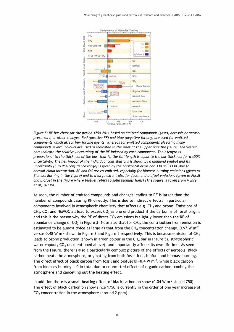
Figure 5: RF bar chart for the period 1750–2011 based on emitted compounds (gases, aerosols or aerosol
precursors) or other changes. Red (positive RF) and blue (negative forcing) are used for emitted
components which affect few forcing agents, whereas for emitted components affecting many
compounds several colours are used as indicated in the inset at the upper part the figure. The vertical
bars indicate the relative uncertainty of the RF induced by each component. Their length is
proportional to the thickness of the bar, that is, the full length is equal to the bar thickness for a ±50%
uncertainty. The net impact of the individual contributions is shown by a diamond symbol and its
uncertainty (5 to 95% confidence range) is given by the horizontal error bar. ERFaci is ERF due to
aerosol–cloud interaction. BC and OC are co-emitted, especially for biomass burning emissions (given as
Biomass Burning in the figure) and to a large extent also for fossil and biofuel emissions (given as Fossil
and Biofuel in the figure where biofuel refers to solid biomass fuels) (The Figure is taken from Myhre
et al, 2013b).
As seen, the number of emitted compounds and changes leading to RF is larger than the
number of compounds causing RF directly. This is due to indirect effects, in particular
components involved in atmospheric chemistry that affects e.g. CH4 and ozone. Emissions of
CH4, CO, and NMVOC all lead to excess CO2 as one end product if the carbon is of fossil origin,
and this is the reason why the RF of direct CO2 emissions is slightly lower than the RF of
abundance change of CO2 in Figure 3. Note also that for CH4, the contribution from emission is
estimated to be almost twice as large as that from the CH4 concentration change, 0.97 W m–2
versus 0.48 W m–2 shown in Figure 3 and Figure 5 respectively. This is because emission of CH4
leads to ozone production (shown in green colour in the CH4 bar in Figure 5), stratospheric
water vapour, CO2 (as mentioned above), and importantly affects its own lifetime. As seen
from the Figure, there is also a particularly complex picture of the effects of aerosols. Black
carbon heats the atmosphere, originating from both fossil fuel, biofuel and biomass burning.
The direct effect of black carbon from fossil and biofuel is +0.4 W m–2, while black carbon
from biomass burning is 0 in total due to co-emitted effects of organic carbon, cooling the
atmosphere and cancelling out the heating effect.
In addition there is a small heating effect of black carbon on snow (0.04 W m–2 since 1750).
The effect of black carbon on snow since 1750 is currently in the order of one year increase of
CO2 concentration in the atmosphere (around 2 ppm).

Monitoring of greenhouse gases and aerosols at Svalbard and Birkenes in 2015 | M-694 | 2016
19
2. Observations of climate gases at the
Birkenes and Zeppelin
Observatories NILU measures 41 climate gases at the Zeppelin Observatory at Svalbard and 2 at Birkenes, in
addition to surface ozone reported in Aas et al. (2016). The results from these measurements,
and analysis are presented in this chapter. Also observations of CO2 since 1989 at Zeppelin
performed by the Stockholm University - Department of Applied Environmental Science (ITM),
are included in the report.
Table 3 summarize the main results for 2015 and the trends over the period 2001-2015. Also
a comparison of the main greenhouse gas concentrations at Zeppelin and Birkenes compared
to annual mean values given in the 5th Assessment Report of the IPCC (Myhre et al. 2013b) is
included.
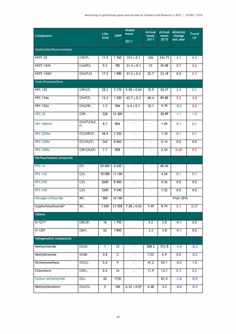
Table 3: Greenhouse gases measured at Zeppelin and Birkenes; lifetimes in years, global warming potential (GWP)
for 100 year horizon, and global mean for 2011 is taken from 5th Assessment Report of the IPCC, Chapter 8 (Myhre
et al, 2013b). Global mean is compared to annual mean values at Zeppelin and Birkenes for 2011. Annual mean for
2015, change last year, the trends per year over the period 2001-2015 is included. All concentrations are mixing
ratios in ppt, except for methane, nitrous oxide and carbon monoxide (ppb) and carbon dioxide (ppm). The
components marked in green are implemented in the programme in 2015, with measurements back to 2010, and
reported for the first time.
Component Life-time
GWP
Global mean
2011
Annual mean 2011
Annual mean 2015
Absolute change
last year
Trend /yr
Carbon dioxide - Zeppelin
CO2 - 1 391 ± 0.2
392.5 401.0 1.6 2.1
Carbon dioxide - Birkenes 397.4 403.9 2.2 -
Methane - Zeppelin
CH4 12.4 28 1803 ± 2
1879.5 1920.2 10.2 5.2
Methane - Birkenes 1895.5 1925.9 8.5 -
Carbon monoxide CO few
months -
- 115.2 113.6 0.4 -1.3
Nitrous oxide N2O 121 265 324 ± 0.1 324.2 328.1 1.1 -
Chlorofluorocarbons
CFC-11* CCl3F 45 4 660 238 ± 0.8 238.3 234.1 -0.9 0.0
CFC-12* CF2Cl2 640 10 200 528 ± 1 531.5 523.4 -2.0 -2.1
CFC-113* CF2ClCFCl2 85 13 900 74.3 ± 0.1 74.6 72.9 -0.6 -0.7
CFC-115* CF3CF2Cl 1 020 7 670 8.37 8.42 8.5 0.0 0.0
Monitoring of greenhouse gases and aerosols at Svalbard and Birkenes in 2015 | M-694 | 2016
20
Component Life-time
GWP
Global mean
2011
Annual mean 2011
Annual mean 2015
Absolute change
last year
Trend /yr
Hydrochlorofluorocarbons
HCFC-22 CHClF2 11.9 1 760 213 ± 0.1 226 244.73 4.7 6.5
HCFC-141b C2H3FCl2 9.2 782 21.4 ± 0.1 23 26.08 0.7 0.6
HCFC-142b* CH3CF2Cl 17.2 1 980 21.2 ± 0.2 22.7 23.18 0.0 0.7
Hydrofluorocarbons
HFC-125 CHF2CF3 28.2 3 170 9.58 ± 0.04 10.9 20.27 2.4 0.1
HFC-134a CH2FCF3 13.4 1 300 62.7 ± 0.3 68.4 89.88 5.5 4.8
HFC-152a CH3CHF2 1.5 506 6.4 ± 0.1 10.1 9.79 -0.3 0.6
HFC-23 CHF3 228 12 400 - - 28.89 1.1 1.0
HFC-365mfc CH3CF2CH2CF3
8.7 804 -
- 1.09 0.1 0.1
HFC-227ea CF3CHFCF3 38.9 3 350 - - 1.10 0.1 0.1
HFC-236fa CF3CH2CF3 242 8 060 - - 0.14 0.0 0.0
HFC-245fa CHF2CH2CF3 7.7 858 - - 2.54 0.20 0.2
Perfluorinated compunds
PFC-14 CF4 50 000 6 630 - - 80.06 - -
PFC-116 C2F6 10 000 11 100 - - 4.54 0.1 0.1
PFC-218 C3F8 2600 8 900 - - 0.56 0.0 0.0
PFC-318 C4F8 3200 9 540 - - 1.52 0.0 0.0
Nitrogen trifluoride NF3 500 16 100 From 2016
Sulphurhexafluoride* SF6 3 200 23 500 7.28 ± 0.03 7.49 8.74 0.3 0.27
Halons
H-1211* CBrClF2 16 1 750 4.2 3.8 -0.1 0.0
H-1301 CBrF3 65 7 800 3.3 3.8 -0.1 0.0
Halogenated compounds
Methylchloride CH3Cl 1 12 - 508.2 512.8 -1.4 -0.3
Methylbromide CH3Br 0.8 2 - 7.02 6.9 0.0 -0.2
Dichloromethane CH2Cl2 0.4 9 - 41.2 54.1 -0.5 1.8
Chloroform CHCl3 0.4 16 - 11.9 13.7 0.3 0.2
Carbon tetrachloride CCl4 26 1730 81.0 -1.6 -0.9
Methylchloroform CH3CCl3 5 160 6.32 ± 0.07 6.48 3.2 -0.6 -0.3

Monitoring of greenhouse gases and aerosols at Svalbard and Birkenes in 2015 | M-694 | 2016
21
Component Life-time
GWP
Global mean
2011
Annual mean 2011
Annual mean 2015
Absolute change
last year
Trend /yr
Trichloroethylene CHClCCl2 - - - 0.549 0.3 -0.2 0.0
Perchloroethylene CCl2CCl2 - - - 2.8 2.4 -0.1 -0.1
Volatile Organic Compounds (VOC)
Ethane C2H6 Ca 78 days* - - 1625.5 34.9 38.7
Propane C3H8 Ca 18 days* - - 503.2 -1.2 7.7
Butane C4H10 Ca 8 days* - - 184.4 -5.6 0.97
Pentane C5H12 Ca 5 days* - - 60.4 -2.8 -0.38
Benzene C6H6 Ca 17 days* - - 68.3 2.5 -3.7
Toluene C6H5CH3 Ca 2 days* - - 24.6 3.6 -2.3
*The lifetimes of VOC and NMHC are strongly dependant on season, sunlight, other components etc. The estimates are global averages given in C. Nicholas Hewitt (ed.): Reactive Hydrocarbons in the Atmosphere, Academic Press, 1999, p. 313. The times series for these are short and the trend is very uncertain.
Greenhouse gases and other climate gases have numerous sources, both anthropogenic and
natural. Trends and future changes in concentrations are determined by their sources and the
sinks, and in section 2.1 are observations and trends of the monitored greenhouse gases with
both natural and anthropogenic sources presented in more detail. In section 2.2 are the
detailed results of the ozone depleting substances with purely anthropogenic sources
presented.
We have used the method described in Appendix II in the calculation of the annual trends,
and also include a description of the measurements at Zeppelin at Svalbard and Birkenes
Observatory in southern Norway in more details. Generally, Zeppelin Observatory is a unique
site for observations of changes in the background level of atmospheric components. All peak
concentrations of the measured gases are significantly lower here than at other sites at the
Northern hemisphere, due to the station’s remote location. Birkenes is closer to the main
source areas. Further, the regional vegetation is important for regulating the carbon cycle,
resulting in much larger variability in the concentration level compared to the Arctic region.

Monitoring of greenhouse gases and aerosols at Svalbard and Birkenes in 2015 | M-694 | 2016
22
2.1 Climate gases with natural and
anthropogenic sources The annual mean concentrations for all gases included in the program for all years are given
in Appendix I, Table A 1 at page 95. All the trends, uncertainties and regression coefficients
are found in Table A 2 at page 95. Section 2.1 focuses on the measured greenhouse gases that
have both natural and anthropogenic sources.
2.1.1 Carbon dioxide at the Birkenes and Zeppelin Observatories
Carbon dioxide (CO2) is the most important anthropogenic greenhouse gas with a radiative
forcing of 1.82 W m-2 since the year 1750, and an increase since the previous IPCC report
(AR4, 2007) of 0.16 Wm-2 (Myhre et al., 2013b). The increase in forcing is due to the increase
in concentrations over these last years. CO2 is the end product in the atmosphere of the
oxidation of all main organic compounds, and it has shown an increase of as much as 40 %
since the pre industrial time (Hartmann et al, 2013). This is mainly due to emissions from
combustion of fossil fuels and land use change. CO2 emissions from fossil fuel burning and
cement production increased by 2.3% in 2013 since 2012, with a total of 9.9±0.5 GtC (billion
tonnes of carbon) equal to 36 GtCO2 emitted to the atmosphere, 61% above 1990 emissions
(the Kyoto Protocol reference year). Emissions are projected to decrease slightly (-0.6%) in
2015 according to Global Carbon Project estimates http://www.globalcarbonproject.org.
NILU started CO2 measurements at the Zeppelin Observatory in 2012 and the results are
presented in Figure 6, together with the time series provided by ITM, University of Stockholm,
back to 1988. ITM provides all data up till 2012 and we acknowledge the effort they have
been doing in monitoring CO2 at the site. Until 2009 the only Norwegian site measuring well-
mixed greenhouse gases (LLGHG) greenhouse gases was Zeppelin, but after upgrading
Birkenes there are continuous measurements of CO2 and CH4 from mid May 2009 also at this
site.
The atmospheric daily mean CO2 concentration measured at Zeppelin Observatory for the
period mid 1988-2015 is presented in Figure 6 upper panel, together with the shorter time
series for Birkenes in the lower panel.

Monitoring of greenhouse gases and aerosols at Svalbard and Birkenes in 2015 | M-694 | 2016
23
The results show continuous increase since the start of the observations at both sites. As can
be seen there are much stronger variability at Birkenes than Zeppelin. At Zeppelin the largest
variability is during winter/spring. For Birkenes hourly mean, (lower panel, grey) it is clear
that the variations are largest during the summer months. In this period, there is a clear
diurnal variation with high values during the night and lower values during daytime. This is
mainly due to changes between plant photosynthesis and respiration, but also the general
larger meteorological variability and diurnal change in planetary boundary layer, particularly
during summer contributes to larger variations in the concentrations. In addition to the
diurnal variations, there are also episodes with higher levels at both sites due to transport of
pollution from various regions. In general, there are high levels when the meteorological
situation results in transport from Central Europe or United Kingdom at Birkenes, and central
Europe or Russia at Zeppelin. The maximum daily mean value for CO2 in 2015 was 433.2 ppm
Figure 6: The atmospheric daily mean CO2 concentration measured at Zeppelin Observatory for the period mid
1988-2015 is presented in the upper panel. Prior to 2012, ITM University of Stockholm provides all data, shown as
orange dots and the green solid line is from the Picarro instrument installed by NILU in 2012. The measurements
for Birkenes are shown in the lower panel, the green line is the daily mean and the hourly mean is shown as the
grey line.
1988
1990
1992
1994
1996
1998
2000
2002
2004
2006
2008
2010
2012
2014
2016
340
350
360
370
380
390
400
410
pp
m
Year
20092010
20112012
20132014
20152016
360
380
400
420
440
460
480
500
pp
m
Year

Monitoring of greenhouse gases and aerosols at Svalbard and Birkenes in 2015 | M-694 | 2016
24
at Birkenes 6th November, and at Zeppelin the highest daily mean value was 410.2 ppm at 6th
December 2015.
Figure 7 shows the development of the annual mean concentrations of CO2 measured at
Zeppelin Observatory for the period 1988-2015 in orange together with the values from
Birkenes in green since 2010. The global mean values as given by WMO in black. The yearly
annual change is shown in the lower panel.
Figure 7: Upper panel: the annual mean concentrations of CO2 measured at Zeppelin Observatory for the period 1988-
2015 shown in orange. Prior to 2012, ITM University of Stockholm provides all data. The annual mean values from
Birkenes are shown as green bars. The global mean values as given by WMO are included in black. The yearly annual
change is shown in the lower panel, orange for Zeppelin, green for Birkenes.

Monitoring of greenhouse gases and aerosols at Svalbard and Birkenes in 2015 | M-694 | 2016
25
The global mean increase for 2014 to 2015 was 2.3 (WMO, 2016). The annual mean values for
Birkenes and Zeppelin are higher than the global mean as, there are more anthropogenic
sources and pollution at the Northern hemisphere. The mixing to the southern hemisphere
takes time, ca 2-3 years. The annual change shown in the lower panel shows an increase of
only 1.6 ppm at Zeppelin since 2014, which is remarkably low compared to global mean
increase and the reason for this would need a thorough study. At Birkenes, the increase since
2014 was 2.2 ppm, in line with the last year’s development and the expectations. The time
series for CO2 at Birkenes is too short to be used in trend calculations.
Key findings for CO2: CO2 concentration has increased all years subsequently, in accordance
with the global mean development and increase of anthropogenic emissions. The new record
levels in 2015 are 401.2 ppm at Zeppelin and 405.1 ppm at Birkenes. The increase from
2014 to 2015 is 1.6 ppm and 2.2 ppm, respectably, compared to global mean which was 2.3
ppm increase. The increase at Zeppelin is lower than expected, and currently there is no
clear explanation for this.
2.1.2 Methane at the Birkenes and Zeppelin Observatories
Our measurements from 2015 reveal a pronounced new record in the observed CH4 level, both
at Zeppelin and Birkenes. Methane (CH4) is the second most important greenhouse gas from
human activity after CO2. The radiative forcing is 0.48 W m-2 since 1750 and up to 2011
(Myhre et al., 2013b), but as high as 0.97 W m–2 for the emission based radiative forcing
(Figure 5, page 18) due to complex atmospheric effects. In addition to being a dominant
greenhouse gas, methane also plays central role in the atmospheric chemistry. The
atmospheric lifetime of methane is approx. 12 years, when indirect effects are included, as
explained in section 1.4.
The main sources of methane include boreal and tropical wetlands, rice paddies, emission
from ruminant animals, biomass burning, and extraction and combustion of fossil fuels.
Further, methane is the principal component of natural gas and e.g. leakage from pipelines;
off-shore and on-shore installations are a known source of atmospheric methane. The
distribution between natural and anthropogenic sources is approximately 40% natural sources,
and 60% of the sources are direct result of anthropogenic emissions. Of natural sources there
is a large unknown potential methane source under the ocean floor, so called methane
hydrates and seeps. Further, a large unknown amount of carbon is bounded in the permafrost
layer in Siberia and North America and this might be released as methane if the permafrost
layer melts as a feedback to climate change.
The average CH4 concentration in the atmosphere is determined by a balance between
emission from the various sources and reaction and removal by free hydroxyl radicals (OH) to
produce water and CO2. A small fraction is also removed by surface deposition. Since the
reaction with OH also represents a significant loss path for the oxidant OH, additional CH4
emission will consume additional OH and thereby increasing the CH4 lifetime, implying further
increases in atmospheric CH4 concentrations (Isaksen and Hov, 1987; Prather et al., 2001).
The OH radical has a crucial role in the tropospheric chemistry by reactions with many
emitted components and is responsible for the cleaning of the atmosphere (e.g. removal of

Monitoring of greenhouse gases and aerosols at Svalbard and Birkenes in 2015 | M-694 | 2016
26
CO, hydrocarbons, HFCs, and others). A stratospheric impact of CH4 is due to the fact that
CH4 contributes to water vapour build up in this part of the atmosphere, influencing and
reducing stratospheric ozone.
The atmospheric mixing ratio of CH4 was, after a strong increase during the 20th century,
relatively stable over the period 1998-2006. The global average change was close to zero for
this period, also at Zeppelin. Recently an increase in the CH4 levels is evident from our
observations both at Zeppelin and Birkenes as well as observations at other sites, and in the
global mean (see e.g. section 2.2.1.1.2 in Hartmann et al, 2013, WMO, 2014).
Figure 8 depicts the daily mean observations of CH4 at Zeppelin since the start in 2001 in the
upper panel and Birkenes since start in 2009 in the lower panel.
Figure 8: Observations of daily averaged methane mixing ratio for the period 2001-2015 at the Zeppelin
Observatory in the upper panel. Grey: all data, orange dots: daily concentrations, black solid line: empirical
modelled background methane mixing ratio (fit does not include transport episodes). The right panel show the
transport of air to Zeppelin the 15th February, where maximum CH4 is observed (see the green circle). Daily
mean observations for Birkenes are shown in the lower panel as green dots.
2001
2002
2003
2004
2005
2006
2007
2008
2009
2010
2011
2012
2013
2014
2015
2016
1800
1850
1900
1950
2000
2050
pp
bv
Year
2001
2002
2003
2004
2005
2006
2007
2008
2009
2010
2011
2012
2013
2014
2015
2016
1800
1850
1900
1950
2000
pp
bv

Monitoring of greenhouse gases and aerosols at Svalbard and Birkenes in 2015 | M-694 | 2016
27
As can be seen from the Figure there has been an increase in the concentrations of CH4
observed at both sites the last years, and in general the concentrations are much higher at
Birkenes than at Zeppelin. The highest ever ambient background CH4 concentration detected
at Zeppelin was on the 15th February 2014. This was 1991.3 ppb, and the transport pattern of
that day shows strong influence from Russian industrial pollution. Fugitive emission from
Russian gas installations is a possible source of this CH4 however, on this particular day, both
CO and CO2 levels were also very high, indicative of an industrial and urban pollution episode.
This year there were several strong episodes, but not with the high value as observed in 2014.
As a part of a research project, we could investigate these in more detail this year, and this is
included in see section 2.1.2.1 at page 30.
For both Zeppelin and Birkenes, the seasonal variations are clearly visible, although stronger
at Birkenes than Zeppelin. This is due longer distance to the sources at Zeppelin, and thus the
sink through reaction with OH dominates the variation. The larger variations at Birkenes are
explained by both the regional sources in Norway, as well as a stronger impact of pollution
episodes from long range transport of pollution from Europe. For the daily mean in Figure 8,
the measurements show very special characteristics in 2010 and 2011 at Zeppelin. As shown,
there is remarkably lower variability in the daily mean in 2011 with fewer episodes than the
typical situation in previous and subsequent e.g. summer/autumn 2012. The reason for this
has been intensively investigated as part of various national and international research
programmes, also at NILU (e.g. Thompson et al, 2016).
At Zeppelin there are now almost 15 years of data, for which the trend has been calculated.
To retrieve the annual trend in the methane for the entire period, the observations have been
fitted by an empirical equation. The fit to the observed methane values are shown as the
black solid line in Figure 8. Only the observations during periods with clean air arriving at
Zeppelin are used in the model, thus the model represents the background level of methane
at the site (see Appendix I for details). This corresponds to an average increase of 5.2 ppb per
year, or ca 0.4% per year, the last years. The pronounced increase started in
November/December 2005 and continued throughout the years 2007 - 2009, and is
particularly evident in the late summer-winter 2007, and summer-autumn 2009. For Birkenes
shown in the lower panel, the time series is too short for trend calculations, but a yearly
increase is evident since the start 2009. There are also episodes with higher levels due to
transport of pollution from various regions. In general, there are high levels when the
meteorological situation results in transport from Central Europe.
The year 2015 showed 1845 ppb CH4 as the new record in global annual mean values (WMO,
2016), and Zeppelin and Birkenes revealed new record levels at both sites. The annual mean
increase in the CH4 levels the last years is visualised in Figure 9 showing the CH4 annual mean
mixing ratio for the period 2001-2015 from Zeppelin (orange) and for Birkenes (green) from
2010-2015. The global mean value given by WMO (WMO, 2016) is included for comparison,
together with the published IPCC global mean value for 2011 (IPCC, 2013).

Monitoring of greenhouse gases and aerosols at Svalbard and Birkenes in 2015 | M-694 | 2016
28
Figure 9: Development of the annual mean mixing ratio of methane in ppb measured at the Zeppelin Observatory
(orange bars) for the period 2001-2015, Birkenes for the period 2010-2015 in green bars, compared to global mean
provided by WMO as black bars (WMO, 2016).
The annual means are based on the measured methane values. Modelled empirical
background values are used, when data is lacking in the calculation of the annual mean. The
diagram in Figure 9 clearly illustrates the increase in the concentrations of methane at
Zeppelin since 2005 a small decrease from 2010 to 2011, and then a new record level in 2015.
The annual mean mixing ratio for 2015 was 1920 ppb, an increase of 10 ppb, compared from
2014 to 2015. The annual mean value for 2015 confirms that there is still a strong increase
from year to year in Arctic methane. The global mean for 2015 was 1945 ppb, with an
increase of 11 ppb from the year before. The increase at Birkenes was slightly weaker for
2014-2015; 8.5 ppb. The increase since 2005 at Zeppelin is 68 ppb (approx. 3.7 %) which is
high compared to the development of the methane mixing ratio in the period from 1999-2005
at Zeppelin, Svalbard and globally. It is also slightly higher than the global mean increase
since 2005 which was 60 ppb, as published in the yearly bulletins by WMO (WMO, 2011, 2012,
2013, 2014, 2015, 2016). The global mean shows an increase since 2006, which over the years
2009-2013 was e.g. 5-6 ppb per year but as high as 9 ppb from 2013-2014 and 12 ppb from
2014-2015, close to what we detected at Zeppelin from 2013-2014.
Larger fluctuations are evident at Zeppelin. This is explained by the distribution of the
sources; there are more sources in the northern hemisphere, and thus more inter-annual
variations. The global mean is lower as this includes all areas of the globe, e.g. remote
locations such as Antarctica and is therefore lower than the values at Zeppelin and Birkenes,
located closer to the sources. Hence, there is a time lag in the development. For comparison,
during the 1980s when the methane mixing ratio showed a strong increase, the annual global
mean change was around 15 ppb per year.
Currently, the observed increase over the last years is not fully explained. The recent
observed increase in the atmospheric methane concentrations has led to enhanced focus and

Monitoring of greenhouse gases and aerosols at Svalbard and Birkenes in 2015 | M-694 | 2016
29
intensified research to improve the understanding of the methane sources and changes
particularly in responses to global and regional climate change. Leaks from gas installations,
world-wide, both onshore and offshore might be an increasing source. Hence, it is essential to
find out if the increase since 2005 is due to high emissions from point sources, or if it is
caused by newly initiated processes releasing methane to the atmosphere e.g. the thawing of
the permafrost layer or processes in the ocean, both related to permafrost and others.
Recent and ongoing scientific discussions point in the direction of increased emissions from
wetlands located both in the tropical region and in the Arctic region. This is also investigated
in a collaboration between NILU and Cicero (Dalsøren et al., 2016). Gas hydrates at the sea
floor are widespread in thick sediments in this area between Spitsbergen and Greenland. If
the sea bottom warms, this might initiate further emissions from this source. This is the core
of the large polar research project MOCA - Methane Emissions from the Arctic OCean to the
Atmosphere: Present and Future Climate Effects3, which started at NILU in October 2013, and
is expected to be finalized by spring 2017 (see http://moca.nilu.no). A few results from this
is included in next the section.
Key findings for Methane – CH4: In 2015 the mixing ratios of methane increased to a new
record level both at Zeppelin, Birkenes and globally. At Zeppelin the annual mean value
reached 1920 ppb with an increase of as much as 10 ppb since 2015. The changes in the last
10 years are large compared to the evolution of the methane levels in the period 1998-2005,
when the change was close to zero both at Zeppelin and globally, after a strong increase
during the mid 20th Century. The methane increase at the Zeppelin observatory from 2005 to
2015, (69 ppb, or around 3.7%) was larger than the global increase in the same period
(approx. 62 ppb, or 3.5 %). The measurements of CH4 at Birkenes showed an annual mean
value for 2015 of 1925 ppb, which is higher than the annual values both for Zeppelin and the
global mean global mean. The increase from 2014 to 2015 at Birkenes was 8.5 ppb. This is
lower than the increase for 2013-2014 which was as high as 15 ppb.
There is a combination of causes explaining the increase in methane the last years, and the
dominating reason is not clear. A probable explanation is increased methane emissions from
wetlands, both in the tropics as well as in the Arctic region, in addition to increases in
emission from the fossil fuel industry. Melting permafrost, both in terrestrial regions and in
marine region, might introduce new possible methane emission sources initiated by the
temperature increase the last years in the Arctic region.
3 http://moca.nilu.no/

Monitoring of greenhouse gases and aerosols at Svalbard and Birkenes in 2015 | M-694 | 2016
30
2.1.2.1 Methane from Arctic Ocean to the atmosphere?
There is an ongoing comprehensive research
project at NILU “MOCA - Methane Emissions
from the Arctic OCean to the Atmosphere:
Present and Future Climate Effects” focusing
on methane from Arctic Ocean to the
atmosphere. This is collaboration with CAGE
(The Centre for Arctic Gas Hydrate,
Environment and Climate, at UiT The Arctic
University of Norway) and Cicero, but lead by
NILU. The driving questions for MOCA are:
I. What is the status and current release of
methane from marine seep sites and
methane hydrates in the Arctic Ocean, and
specifically around Svalbard?
II. How are these processes depending on
trends in sea temperature and annual
variations?
III. Where are the most important areas in
the Arctic Ocean which could constitute a
possible source of atmospheric methane,
now and in the future?
IV. What is the present CH4 emission from
the seabed to the atmosphere?
V. What is the most likely change in flux, the next 50 and 100 years under realistic climate
scenarios? And what is the global effect of this?
VI. What is the ocean temperature threshold for large changes in emission of methane
from hydrates?
In this project we use integrated approaches to answer these questions. Figure 10 shows the
exploratory platforms involved. Comprehensive measurement campaigns involving ship,
aircrafts and Zeppelin have been performed. We have used additionally we use models both
atmospheric chemistry, methane hydrates modelling at sea floor, and and climate models.
What are gas hydrates?
Large amounts of natural gas, mainly methane,
are stored in the form of hydrates in continental
margins worldwide,
particularly, in the
Arctic. Gas hydrate
consists of ice-like
crystalline solids of
water molecules
encaging gas molecules, and is often referred to
as ‘the ice that burns’.
What are seeps? Cold seeps are locations where hydrocarbons are emitted from sub-seabed gas reservoirs into the ocean. This can be both from petroleum reservoirs and methane hydrates. The illustration is gas bubbles rising 800 m up from Vestnesa Ridge, offshore Svalbard (Smith et al. 2014). http://cage.uit.no

Monitoring of greenhouse gases and aerosols at Svalbard and Birkenes in 2015 | M-694 | 2016
31
Figure 10: Field campaign and measurement platforms at the sea floor, in the water column, and in the
atmosphere west of Svalbard in June-July 2014. Seeps on the seafloor, represented here by swath bathymetry,
release gas bubbles that rise through the water column. The Research Vessel Helmer Hanssen detected gas bubbles
and collected water samples at various depths, and provided online atmospheric CH4, CO and CO2 mixing ratios
and discrete sampling of complementary trace gases and isotopic ratios. The Facility of Airborne Atmospheric
Measurements (FAAM) aircraft measured numerous gases in the atmosphere, and an extended measurement
program was performed at the Zeppelin Observatory close to Ny-Ålesund. Data from Zeppelin was used for
comparison to detect possible oceanic sources.
We have used different state-of-the art models to assess and understand the variation in
Arctic methane, to investigate potential oceanic sources in various regions, in particular
methane hydrates and cold seeps. First, results are presented in Myhre et al (2016), Pisso et
al (2016), Thompson et al (2016), and some information can be found here:
http://forskning.no/havforskning-klima-arktis/2016/05/metan-slipper-ikke-ut-av-polhavet-
om-sommeren.
As a part of this, we included s detailed analysis of the 2015 methane time series at Zeppelin,
using the FLEXPART model at NILU. Detail information about sources regions for 5 episodes
are included in Figure 11.

Monitoring of greenhouse gases and aerosols at Svalbard and Birkenes in 2015 | M-694 | 2016
32
Ep. 1: 22 February: Main source region
was industrial area in Northern
Russia/Siberia.
Ep. 2: 11 April: Main source region was
industrial area in Northern
Russia/Siberia.
Ep. 3: 29 July: Oceanic areas, and area
with oil and gas installations, North-
West in Russia (close to Novaja Semlja)
Ep. 4: 26 October: Arctic Ocean and
Norther-East Russia.
Ep. 5: 13 November: Central Russian
and eastern European pollution.
Figure 11: Illustration of impact on CH4 at Zeppelin from different regions in the Arctic by use of FLEXPART (See also
Pisso et al, 2016).
1. Jan
uary
201
5
1. M
arch
201
5
1. M
ay 2
015
1. July 20
15
1. S
epte
mbe
r 201
5
1. N
ovem
ber 2
015
1900
1950
5
4
3
2
pp
bv
1

Monitoring of greenhouse gases and aerosols at Svalbard and Birkenes in 2015 | M-694 | 2016
33
2.1.3 Non-methane hydrocarbons (NMHC) at the Zeppelin Observatory
Atmospheric NMHC oxidation contributes to the production of tropospheric ozone and
influences photochemical processing, both impacting climate and air quality. Sources of
NMHCs (here ethane, propane, butane, pentane) include natural (mostly geological but also
from wild fires) and anthropogenic (fossil fuels) ones. CH4 and NMHCs are co-emitted from oil
and natural gas sources, for CH4 to ethane the mass ratio varies from 7 to 14 (Helmig et al,
2016). The atmospheric ethane budget is not well understood and state-of-the-art
atmospheric models underestimate ethane-mixing ratios, implying that current emission
inventories require additional sources to balance the global atmospheric ethane budget.
Helmig et al (2016) showed, from long-term observations of ethane from a global network
that concentrations are increasing (since circa 2010), and that there is a strong latitudinal
gradient, with the highest abundances observed in the Arctic, and a steep decline towards
the south. They concluded that emissions from North American oil and natural gas
development are the primary cause of increasing concentrations in recent years. However,
there might be other factors. A recent study by Nicewonger et al (2016) used analysis of polar
ice cores to estimate the pre-industrial emissions and concluded that natural ethane
emissions from geologic seeps contributed significantly to the preindustrial ethane budget.
Etiope and Ciccioli (2009) suggested that a substantial part of the missing ethane source can
be attributed to gas seepage, but they did not include the Arctic in their study.
Figure 12 shows the daily mean observations of the four NMHCs included in the programme,
ethane, propane, butane and pentane, at Zeppelin since the start in September 2010.
Figure 12: Observations of daily averaged mixing ratio of benzene (upper panel) and toluene (lower panel) for
the period September 2010 – 2015 at the Zeppelin Observatory.
2010
2011
2012
2013
2014
2015
2016
0
100
200
300
4000
250500750
10001250
0
1000
2000
3000
1000
2000
3000
Pentane
pp
t v
Year
Butane
pp
t v
Propane
pp
t v
Ethane
pp
t v

Monitoring of greenhouse gases and aerosols at Svalbard and Birkenes in 2015 | M-694 | 2016
34
Due to the short lifetimes ranging from a few days for pentane to 2-3 months for ethane, the
annual cycles are very strong. The time series are too short for calculation of trends, but
annual mean development are given in Figure 13.
The data coverage the compounds are relatively low over the period, hence the development
is uncertain. Still, it seems that the development of the annual means since 2011
Figure 13: Development of the annual means of the measured non-methane hydrocarbons at the Zeppelin
Observatory for the period 2011-2015. Upper panel in dark green: ethane, mid-panel propane, and lower panel
Butane and Pentane.

Monitoring of greenhouse gases and aerosols at Svalbard and Birkenes in 2015 | M-694 | 2016
35
demonstrates that ethane has increased and have a different development than the more
heavy NMHCs in the lower panels, although many of the sources are considered as the same.
Hence, this can indicate that some of dominating ethane sources, with less content of the
heavier NMHC is increasing, compared to the others.
Key findings – NMHC: The hydrocarbon ethane, often co-emitted with fossil fuel methane, is
increasing at Zeppelin, but toluene and benzene (see next section), show stable values since
2014. These are short lived climate gases important for the levels of aerosols, ozone, CO and
contribute to CO2 and others, but with low direct greenhouse gas effects.
2.1.4 Other Volatile Organic Compounds (VOC) at the Zeppelin Observatory
Volatile Organic Compounds (VOCs) are a large group of carbon-based compounds that have a
high vapor pressure and easily evaporate at room temperature. At Zeppelin two important
VOCs are measured, benzene and toluene, which belong to a group of VOCs found in
petroleum hydrocarbons, such as gasoline. The compounds have attracted much attention
since they are considered a strong carcinogen (especially benzene), but they are also
important for climate. The VOCs have relatively short atmospheric lifetimes and small direct
impact on radiative forcing. However, anthropogenic secondary organic aerosols (SOA) are
formed from photo oxidation of benzene and toluene (Ng et al., 2007), which indirectly
impacts the climate. The SOA formation from these VOCs is most effective under low-NOx
conditions and when ambient concentration of organic aerosols is high. Thus, benzene and
toluene influence climate through their production of secondary organic aerosols and their
involvement in photochemistry, i.e., production of O3 in the presence of light.
Figure 14 depicts the daily mean observations of benzene and toluene at Zeppelin since the
start in September 2010.

Monitoring of greenhouse gases and aerosols at Svalbard and Birkenes in 2015 | M-694 | 2016
36
Figure 14: Observations of daily averaged mixing ratio of benzene (upper panel) and toluene (lower panel) for
the period September 2010 – 2015 at the Zeppelin Observatory.
As can be seen from the Figure there is strong annul variations, mainly explained by the
reactions induced by sunlight. For both component there seem to be a decreasing trend, but
this is far too early to conclude, due to the short time series available.
The annual means of benzene and toluene for the period 2010-2015 is presented in Figure 15.
The period 2010 to 2015 was relatively stable for both components, with strong episodes
during wintertime due to transport of urban polluted air from lower latitudes.
2010
2011
2012
2013
2014
2015
2016
0
50
100
150
200
250
3000
50
100
150
200
250
300
Toluene
pp
t v
Year
Benzene
pp
t v

Monitoring of greenhouse gases and aerosols at Svalbard and Birkenes in 2015 | M-694 | 2016
37
Figure 15: Development of the annual means of benzene (deep brown) and toluene (dark red) for the period
September 2011 – 2015 at the Zeppelin Observatory.
2.1.5 Nitrous Oxide at the Zeppelin Observatory
Nitrous Oxide (N2O) is a greenhouse gas with both natural and anthropogenic sources. The
sources include oceans, tropical forests, soil, biomass burning, cultivated soil and use of
particular synthetic fertilizer, and various industrial processes. There are high uncertainties
in the major soil, agricultural, combustion and oceanic sources of N2O. Also frozen peat soils
in Arctic tundra is reported as a potential source (Repo et al., 2009), but recent studies lead
by NILU identify tropical and sub-tropical regions as the largest source regions (Thompson et
al, 2013). N2O is an important greenhouse gas with a radiative forcing of 0.17 W m-2 since
1750 contributing around 6 % to the overall well-mixed greenhouse gas forcing over the
industrial era. N2O is also the major source of the ozone-depleting nitric oxide (NO) and
nitrogen dioxide (NO2) in the stratosphere, thus the component is also influencing the
stratospheric ozone layer. The Assessment of the ozone depletion (WMO, 2011) suggests that
current emissions of N2O are presently the most significant substance that depletes ozone.
N2O has increased from around 270 ppb prior to industrialization and up to an average global
mean of 328.0 ppb in 2015 (WMO, 2016). In 2009, NILU installed a new instrument at Zeppelin
measuring N2O with high time resolution of 15 minutes. The instrument was in full operation
in April 2010 and the results for 2010 -2015 are presented in Figure 16, with the global mean
included as horizontal lines for each year.

Monitoring of greenhouse gases and aerosols at Svalbard and Birkenes in 2015 | M-694 | 2016
38
Figure 16: Measurements of N2O at the Zeppelin Observatory for 2010-2015.The grey shaded areas are global
annual mean, with the given uncertainty (WMO, 2011, 2012, 2013, 2014, 2015, 2016)
The time series is too short for trend calculations, but according to WMO (WMO, 2016) the
global mean increase of 1 ppb since 2014. Annual mean for Zeppelin in 2015 was 328.1 with a
standard deviation of 0.66 ppb. Due to instrumental problems there was a higher uncertainty
this year, compared to earlier periods. As can be seen a high variability in 2015 is evident. As
a part of ICOS-Norway a Norwegian infrastructure project funded by Norwegian Research
Council, a new instrument is purchased and installed autumn 2016. The two instruments will
run in parallel to ensure overlap and consistent long time series.
Key findings Nitrous Oxide –N2O: The global mean level of N2O has increased from around
270 ppb prior to industrialization and up to an average global mean of 328.1 ppb in 2015,
which is new record level after an increase of 0.7 ppb since 2014
2.1.6 Methyl Chloride at the Zeppelin Observatory
Methyl chloride (CH3Cl) is the most abundant chlorine containing organic gas in the
atmosphere, and it contributes approx. 16% to the total chlorine from the well-mixed gases in
the troposphere (WMO, 2011). The main sources of methyl chloride are natural, and
dominating source is thought to be emissions from warm coastal land, particularly from
tropical islands are shown to be a significant source but also algae in the ocean, and biomass
burning. Due to the dominating natural sources, this compound is not regulated through any
of the Montreal or Kyoto protocols, but is an important natural source of chlorine to the
stratosphere. To reach the stratosphere, the lifetime in general needs to be in the order of 2-
4 years to have significant chorine contribution, but this is also dependant on the source
strength and their regional distribution. Methyl chloride has relatively high mixing ratios, and
contributes to the stratospheric chlorine burden.
1. January 2010
1. July 2010
1. January 2011
1. July 2011
1. January 2012
1. July 2012
1. January 2013
1. July 2013
1. January 2014
1. July 2014
1. January 2015
1. July 2015
1. January 2016
323
324
325
326
327
328
329
330
pp
b

Monitoring of greenhouse gases and aerosols at Svalbard and Birkenes in 2015 | M-694 | 2016
39
The results of the measurements of this substance for the period 2001-2015 are shown in
Figure 17.
Figure 17: Observations of methyl chloride, CH3Cl, for the period 2001-2015 at the Zeppelin Observatory. Dots: daily
averaged concentrations from the observations, solid line: empirical modelled background mixing ratio.
The lifetime of the compound is only one year resulting in large seasonal fluctuations, as
shown in the Figure, responds rapid to changes in emissions. There is a decrease the last
years, but this seems to relax in 2011-2012, and a strong increase was detected in 2013.
However, it is positive to note that in 2014, the levels were lower, back on the same
concentration as in 2012, and a further decrease in 2015, see also Figure 18 with the annual
means.
The trend over period 2001-2015 is -0.27 ppt/year. The annual means of methyl chloride for
the period 2001-2015 is presented in Figure 18. The period 2002-2009 was relatively stable,
but since 2009 there is larger variability. From 2009 to 2015 there was an increase of more
than 30 ppt in our data corresponding to an increase of 20%. 2015 showed a reduction
compared to 2014, and since 2009 a reduction of 13% is detected. The reasons to this are not
clear, and sources resulting the rapid observed changed the last years will be investigated at
NILU the coming year. A closer study of source variation for this compound is also
recommended by WMO (WMO, 2011), as the sources are also related to atmospheric
temperature change and ocean.
2001
2002
2003
2004
2005
2006
2007
2008
2009
2010
2011
2012
2013
2014
2015
2016
400
450
500
550
600
650
Daily concentrations of CH3Cl
Model
pp
t v
Year

Monitoring of greenhouse gases and aerosols at Svalbard and Birkenes in 2015 | M-694 | 2016
40
Figure 18: Development of the annual means methyl chloride measured at the Zeppelin Observatory for the period
2001-2015.
2.1.7 Methyl bromide - CH3Br at the Zeppelin Observatory
The sources of methyl bromide (CH3Br) are both from natural and anthropogenic activities.
The natural sources such as the ocean, plants, and soil, can also be a sink for this substance.
Additionally there are also significant anthropogenic sources; it is used in a broad spectrum of
pesticides in the control of pest insects, nematodes, weeds, pathogens, and rodents. Biomass
burning is also a source and it is used in agriculture primarily for soil fumigation, as well as
for commodity and quarantine treatment, and structural fumigation. Even though methyl
bromide is a natural substance, the additional methyl bromide added to the atmosphere by
humans contributes to the man-made thinning of the ozone layer. Total organic bromine from
halons and methyl bromide peaked in 1998 and has declined since. The tropospheric
abundance of bromine is decreasing, and the stratospheric abundance is no longer increasing
(WMO, 2011).
The results of the daily averaged observations of this compound for the period 2001-2015 are
shown in Figure 19. A relatively large change is evident after the year 2007, a reduction of
approx. 20% since the year 2005 at Zeppelin. Methyl bromide is a greenhouse gas with a
lifetime of 0.8 years and it is 2 times stronger greenhouse gas than CO2 (Myhre et al, 2013b) if
the amount emitted of both gases were equal. The short lifetime explains the stronger annual
and seasonal variations of this compound.

Monitoring of greenhouse gases and aerosols at Svalbard and Birkenes in 2015 | M-694 | 2016
41
Figure 19: Observations of methyl bromide, CH3Br, for the period 2001-2015 at the Zeppelin Observatory. Dots: daily
averages mixing ratios from the observations, solid line: empirical modelled background mixing ratio.
For the period 2001-2015 there is a reduction in the mixing ratio of -0.18 ppt per year, with a
relaxation in the trend the last years. However, note that the observed changes are small
(approx. 1.7 ppt since 2005).
The development of the annual means for the period 2001-2015 is presented in Figure 20,
clearly illustrating the decrease in the last years. In general atmospheric amounts of methyl
bromide have declined since the beginning in 1999 when industrial production was reduced as
a result of the Montreal protocol. The global mean mixing ratio was 7.3-7.5 ppt in 2011 (Myhre
et al, 2013b), slightly lower than at Zeppelin. The differences are explained by slower inter
hemispheric mixing. The recent reduction is explained by considerable reduction in the use of
this compound; in 2008 the use was 73% lower than the peak year in late 1990s (WMO, 2011).
Figure 20: Development of the annual means of methyl bromide (in ppt) measured at the Zeppelin Observatory
for the period 2001-2015.
2001
2002
2003
2004
2005
2006
2007
2008
2009
2010
2011
2012
2013
2014
2015
2016
6
7
8
9
10
11
Daily concentrations of CH3Br
Model
pp
t v
Year

Monitoring of greenhouse gases and aerosols at Svalbard and Birkenes in 2015 | M-694 | 2016
42
2.1.8 Carbon monoxide at the Zeppelin Observatory
Atmospheric Carbon monoxide (CO) sources are the oxidation of various organic gases as
volatile organic compounds (VOC) emitted from fossil fuel, biomass burning, and also
oxidation of methane is important. Additionally, emissions from plants, fires and ocean are
important sources. CO is not considered as a direct greenhouse gas, mostly because it does
not absorb terrestrial thermal IR energy strongly enough. However, CO is able to modulate
the level of methane and production of tropospheric ozone, which are both very important
greenhouse gas and hence CO is considered as a relevant climate. CO is closely linked to the
cycles of methane and ozone and, like methane; CO plays a key role in the control of the OH
radical.
CO at Zeppelin is include in the national monitoring programme and the observed CO mixing
ratios for the period September 2001-2015 are shown in Figure 21.
Figure 21: Observations of carbon monoxide (CO) from September 2001 to 31.12.2015 at the Zeppelin
observatory. Red dots: daily averaged observed mixing ratios. The solid line is the modelled background mixing
ratio.
The concentrations of CO show characteristic seasonal variations. This seasonal cycle is driven
by variations in OH concentration as a sink, emission by industries and biomass burning, and
transportation on a large scale. As seen from the Figure there are also peak values due to
long-range transport of polluted air to Zeppelin and the Arctic. The highest mixing ratio of CO
ever observed at Zeppelin; is 217.2 ppb on the 2nd of May 2006. These peak values are due to
transport of polluted air from lower latitudes; urban pollution (e.g. combustion of fossil fuel)
and in spring 2006 it was from agricultural fires in Eastern Europe. The maximum in 2015 was
on 10th of April; 170.1 ppb. The maximum value is caused by transport of pollution from
Central Russia, and also CH4 and CO2 had yearly maximum value this day, see Figure 8 and
also section 2.1.2.1 for comments to this episode. We calculated a trend at Zeppelin of -1.3
ppb per year for the period 2001-2015.
CO has a clear annual cycle with a late winter (February/March) maximum and a late summer
(August) minimum, but for the 2015 data the month of July differs slightly from the expected
behaviour, a pattern recognized also for the 2014 data. Where in summer usually a decline in
the CO concentration is expected, the measurements shows elevated values of CO for the air
arriving at measured at Zeppelin Observatory in July.
2002
2003
2004
2005
2006
2007
2008
2009
2010
2011
2012
2013
2014
2015
2016
50
75
100
125
150
175
200
225
250
pp
bv
Year

Monitoring of greenhouse gases and aerosols at Svalbard and Birkenes in 2015 | M-694 | 2016
43
Figure 22: Development of the annual means of CO measured at the Zeppelin Observatory for the period 2001-2015.
CO is an excellent tracer for transport of smoke from fires (biomass burning, agricultural- or
forest fires). The elevated concentrations in July 2015 are related to long-range transport of
smoke and ash from wildfires in Canada and Alaska. An analyse of the meteorological
situation in the first two weeks of July 2015 shows a synoptically high pressure area over
Greenland and Canada, with easterly wind direction from Canada towards the northwest, and
air masses further arriving in the Arctic via the polar area. 7-days backwards trajectories
from the FLEXTRA model, Figure 23, illustrates the synoptical situation on July 10th.

Monitoring of greenhouse gases and aerosols at Svalbard and Birkenes in 2015 | M-694 | 2016
44
Figure 23: Upper panel: 7-days backwards trajectories from the FLEXTRA model and the synoptical situation on
July 10th. Lower panel: the smoke as detected from the MODIS satellite instrument and spread out over North
America on July 3rd 2015 (left) and visible above the Svalbard Islands on July 10th (right)
The increased CO concentrations arises as a result of air masses arriving at Zeppelin
Observatory is polluted with smoke and particles from more than 200 individual forest fires
across British Columbia, Saskatchewan, and Alberta in July 2015, centred in the northwest of
the continent. In western Canada, more than three times the area that’s normally burned was
affected. (http://www.npr.org/2015/07/11/421995880/wildfires-in-canada-and-alaska-
drive-thousands-from-homes). High record temperatures in most of Alaska also underpinned
the situation. The figure also shows the smoke as detected from the MODIS satellite
instrument and spread out over North America on July 3rd 2015 (left) and visible above the
Svalbard Islands on July 10th (right). The situation lasted until August 8, when the wind in the
Arctic shifted to a more southerly direction again bringing air masses with CO concentrations
close to the expected average for the season to Zeppelin.
Both summer 2014 and 2015 have shown similar patterns in fluctuations in CO concentration,
but it is currently not possible to conclude whether this is due to long term changes in
synoptic and long-range transport situations, and/or changes in the frequency and magnitude
of fires in the forest fire season. Smoke from wildfires is often injected in the stratosphere
and can be transported around the globe with the prevailing jet streams. Soot can stay in the
atmosphere for years. The Zepplin Observatory is a unique station in the Arctic context and it

Monitoring of greenhouse gases and aerosols at Svalbard and Birkenes in 2015 | M-694 | 2016
45
is thus very important to facilitate the provision of long time series from this observatory for
monitoring the situation.
The development of the annual means for the period 2001-2015 are presented in Figure 22,
clearly illustrating a maximum in the year of 2003. In general the CO concentrations
measured at Zeppelin show a decrease during the period 2003 to 2009, and stable levels the
last years with a small peak in 2010.

Monitoring of greenhouse gases and aerosols at Svalbard and Birkenes in 2015 | M-694 | 2016
46
2.2 Greenhouse gases with solely
anthropogenic sources All the gases presented in this chapter have solely anthropogenic sources. These are purely
man-made greenhouse gases and are CFCs, HCFCs, HFCs, SF6 and halons, and most of these
gases did not exist in the atmosphere before the 20th century. All these gases except for SF6
are halogenated hydrocarbons. Although the gases have much lower concentration levels than
most of the natural gases mentioned in the previous section, they are strong infrared
absorbers, many of them with extremely long atmospheric lifetimes resulting in high global
warming potentials; see Table 3. Together as a group, the gases contribute to around 12% to
the overall global radiative forcing since 1750 (Myhre et al, 2013b). The annual mean
concentrations for all the gases included in the monitoring program for all years are given in
Appendix I, Table A 1 at page 95, while all trends, uncertainties and regression coefficients
are found in Table A 2 at page 95.
Some of these gases are ozone depleting, and consequently regulated through the Montreal
protocol. Additional chlorine and bromine from CFCs, HCFCs and halons added to the
atmosphere contributes to the thinning of the ozone layer, allowing increased UV radiation to
reach the earth's surface, with potential impact not only to human health and the
environment, but to agricultural crops as well. In 1987 the Montreal Protocol was signed in
order to reduce the production and use of these ozone-depleting substances (ODS) and the
amount of ODS in the troposphere reached a maximum around 1995. The amount of most of
the ODS in the troposphere is now declining slowly and one expects to be back to pre-1980
levels around year 2050. In the stratosphere the peak is reached somewhat later, around the
year 2000, and observations until 2004 confirm that the level of stratospheric chorine has not
continued to increase (WMO, 2011).
The CFCs, consisting primarily of CFC-11, -12, and -113, accounted for ~62% of total
tropospheric chlorine in 2004 and accounted for a decline of 9 ppt chlorine from 2003-2004
(or nearly half of the total chlorine decline in the troposphere over this period) (WMO, 2011).
There are two generations of substitutes for the CFCs, the main group of the ozone depleting
substances. The first generation substitutes is now included in the Montreal protocol as they
also deplete the ozone layer. This comprises the components called HCFCs listed in Table 3.
The second-generation substitutes, the HFCs, are included in the Kyoto protocol. The general
situation now is that the CFCs have started to decline, while their substitutes are increasing,
and many of them have a steep increase.
2.2.1 Chlorofluorocarbons (CFCs) at Zeppelin Observatory
This section includes the results of the observations of the CFCs: CFC-11, CFC-12, CFC-113,
and CFC-115. These are the main ozone depleting gases, and the anthropogenic emissions
started around 1930s and were restricted in the first Montreal protocol. The main sources of
these compounds were foam blowing, aerosol propellant, temperature control (refrigerators),
solvent, and electronics industry. The highest production of the observed CFCs was around
1985 and maximum emissions were around 1987. The lifetimes of the compounds are long, as

Monitoring of greenhouse gases and aerosols at Svalbard and Birkenes in 2015 | M-694 | 2016
47
given in Table 3, and combined with strong infrared absorption properties, the GWP is high.
Figure 24 shows the daily averaged observed mixing ratios of these four CFCs.
The instrumentation employed at Zeppelin is not in accordance with recommendations and
criteria of AGAGE for measurements of CFCs, and there are relatively high uncertainties in
the observations of these compounds, see also Appendix I. As a result, the trends are
connected with large uncertainties. From September 2010, new and improved
instrumentation was installed at Zeppelin providing more accurate observations of these
compounds. The higher precisions are clearly visualised in Figure 24, but due to several
severe instrumental problems in 2015, there are few days with measurements of these
compounds4.
Figure 24: Daily averaged mixing ratios of the monitored CFCs: CFC-11 (dark blue), CFC-12 (red), CFC-113 (green)
and CFC-115 (light blue) for the period 2001-2015 at the Zeppelin observatory. The solid lines are modelled
background mixing ratio.
The trends per year for the substances CFC-11, CFC12 and CFC-113 given in Table 3 are all
negative, and the changes in the trends are also negative, indicating acceleration in the
decline4. For the compound CFC-115, the trend is still slightly positive, +0.02 ppt/year, and
there is a new increase last years, after a stable period. However, it is important to note the
low data coverage the last year, and hence a higher uncertainty. In total, the development of
4 The current instrumentation is not in accordance with recommendations and criteria of AGAGE for measurements
of the CFCs and there are larger uncertainties in the observations of this compound, see also Appendix I. This is also
why these compounds are very sensitive to instrumental problems.
2001
2002
2003
2004
2005
2006
2007
2008
2009
2010
2011
2012
2013
2014
2015
2016
7.5
8.0
8.5
9.0
70
75
80
85
90520
540
560
580
600
240
260
280
300
CFC-115
pp
t v
Year
CFC-113
pp
t v
CFC-12
pp
t v
CFC-11
pp
t v

Monitoring of greenhouse gases and aerosols at Svalbard and Birkenes in 2015 | M-694 | 2016
48
the CFC levels at the global background site Zeppelin is very promising, and as expected in
accordance with the compliance of the Montreal protocol.
The development of the annual means for all the observed CFCs is shown in Figure 25. The
global annual mean of 2011 as given in IPCC (Chapter 8, Myhre et al, 2013b) is included as
black bars for comparison. As can be seen, the concentrations at Zeppelin are very close to
the global mean for these compounds, as the lifetimes are long and there are hardly any
present-day emissions.
Figure 25: Development of the annual means all the observed CFCs at the Zeppelin Observatory for the period 2001-
2015. Upper left panel: CFC-11, upper right panel: CFC-12, lower left panel: CFC-113, lower right panel: CFC-115.
See Appendix I for data quality and uncertainty. The global annual mean as given in IPCC (Chapter 8, Myhre et al,
2013b) is included as grey bars. All units are ppt.
According to WMO (WMO, 2011) the global mean mixing ratios of CFC-11 are decreasing with
approximately 2.0 ppt +/-0.01 ppt. This is in accordance with our results at Zeppelin (2.1
ppt/year). CFC-12 (the red diagram) has high GWP, 10200, the third highest of all gases
observed at Zeppelin. The global averaged atmospheric mixing ratio of CFC-12 has been
decreasing at a rate of 0.5% over the year 2004-2008 (WMO, 2011). This fits well with our
observations as CFC-12 has the maximum in 2003-2004. There is a clear reduction the last
years of -23 ppt since the maximum year 2005.
Key findings – CFCs: In total the development of the CFC gases measured at the global
background site Zeppelin give reason for optimism. The concentration of the observed CFCs,
CFC-11, CFC-12 and CFC-113 are declining. The mixing ratios of these gases are now
reduced with approx. 9.6%, 4.3% and 10.5% respectively since the start in 2001. CFC-115

Monitoring of greenhouse gases and aerosols at Svalbard and Birkenes in 2015 | M-694 | 2016
49
seems to have stabilized but was in 2015 slightly higher than in 2014, and has a total
increase of 2,8% over the whole period.
2.2.2 Hydrochlorofluorocarbons (HCFCs) at Zeppelin Observatory
This section includes the observations of the following components: HCFC-22, HCFC-141b and
HCFC-142b. These are all first generation replacement gases for the CFCs and their lifetimes
are rather long, see Table 3. The main sources of these gases are temperature control
(refrigerants), foam blowing and solvents, as for the CFCs, which they are supposed to
replace. All these gases are regulated through the Montreal protocol as they all contain
chlorine. The use of the gases is now frozen, but they are not completely phased out. The
gases they have potentially strong warming effects, depending on their concentrations and
absorption properties; their GWPs are high (see Table 3). The compound HCFC-142b has the
highest GWP of these, and the warming potential is 1980 times stronger than CO2, per kg gas
emitted. These gases also contain chlorine, and thus are contributing to the depletion of the
ozone layer.
The daily averaged observations of these gases are shown in Figure 26 for the period
2001-2015.
Figure 26: Daily average mixing ratios of the monitored HCFCs: HCFC-22 (red), HCFC-141b (dark blue) HCFC-142b
(green) for the period 2001-2015 at the Zeppelin observatory. The solid lines are modelled background mixing
ratios. All units are ppt.
2001
2002
2003
2004
2005
2006
2007
2008
2009
2010
2011
2012
2013
2014
2015
2016
15
20
25
15
20
25
30150
175
200
225
250
275
HCFC-142b
pp
t v
Year
HCFC-141b
pp
t v
HCFC-22
pp
t v

Monitoring of greenhouse gases and aerosols at Svalbard and Birkenes in 2015 | M-694 | 2016
50
The trends per year for the compounds HCFC-22, HCFC-141b and HCFC-142b are all positive
over the period. HCFC-22 is the most abundant of the HCFCs and is currently increasing at a
rate of 6.5 ppt/year over the period 2001-2015. The concentration of the two other HCFCs
included are a factor of ten lower, and also the annual increase is about a factor ten lower;
HCFC-141b and HCFC-142b have increased by 0.6 ppt/yr and 0.7 ppt/year, respectively over
the same period. Last years’ HCFC-142b show a very positive development, with no significant
changes since 2011, and even slight decrease from 2014-2015. This is illustrated better in
Figure 27, which shows the annual means for the full period for the three compounds, clearly
illustrating the development; a considerable increase over the period, but for HCFC142b
reveal a stabilisation over the last years. With lifetimes in the order of 10-20 years, it is
central to continue monitoring the development of these compounds for many years to come
as they have an influence both on the ozone layer and are strong climate gases. The global
annual mean of 2011 as given in IPCC (Chapter 8, Myhre et al, 2013b) is included as black bars
for comparison. As can be seen, the development and concentrations at Zeppelin are ca 2-3
ppt ahead of the global mean.

Monitoring of greenhouse gases and aerosols at Svalbard and Birkenes in 2015 | M-694 | 2016
51
Figure 27: Development of the annual means the observed HCFCs at the Zeppelin Observatory for the period
2001-2015. Red: HCFC-22, Blue: HCFC-141b, and green: HCFC-142b. All units are ppt. The global annual mean in
2011 as given in IPCC, Chapter 8 (Myhre et al, 2013b) are included as black bars.
Key findings HCFCs: HCFCs: The CFC substitutes HCFC-22, HCFC-141b and HCFC-142b have
a strong increase in the measured at Zeppelin from 2001-2015. HCFC-22, used for
refrigeration equipment and foam blowing, had the largest growth rate. This is the most
abundant of the HCFCs and its mixing ratio at Zeppelin increased by a rate of 6.5 ppt/year
which is almost 4% per year, and the increase is as much as a 52% since 2001. HCFC-142b had
the strongest relative increase with more than 61% since 2001, but the concentration is about
a factor 10 lower than HCFC-22, and hence the climate effect is weaker as the GWP is circa
the same.

Monitoring of greenhouse gases and aerosols at Svalbard and Birkenes in 2015 | M-694 | 2016
52
2.2.3 Hydrofluorocarbons (HFCs) at Zeppelin Observatory
The substances called HFCs are the so called second generation replacements of CFCs, which
means that they are considered as better alternatives to the CFCs with respect to the ozone
layer than HCFCs. However, many of these are strong greenhouse gases. Even if these
compounds are better alternatives for the protection of the ozone layer as they do not
contain chlorine or bromine, they are still problematic as they are highly potent greenhouse
gases. 1 kg of the gas HFC-125 is as much as 3170 times more powerful greenhouse gas than
CO2 (See Table 3). However, their mixing ratios are currently rather low, but the background
mixing ratios are increasing rapidly, except for HFC-152a, see Figure 28. Last period there has
been a great focus on these and expansion of the Montreal protocol to reduce these (see also
section 1.2). This was agreed in Kigali, October 2016, and an important step to prevent
further global warming. Presently, the contribution to global warming posed by these
compounds are very limited. However, many of these compounds have a very strong increase,
as documented in our measurements presented in this section. At the same time, the
compounds are strong infrared absorbers, with high GWP (see Table 3 at page 19) hence it is
crucial to reduce the use in the future, to prevent further warming by emissions of new
greenhouse gases.
This sub-section includes measurements of the components: HFC-125, HFC-134a, and HFC-
152a with lifetimes in the order of 1.5-29 years, over the period 2001-2015. Additionally, the
program was extended with new compounds in 2015. These are HFC-23, HFC-365mfc, HFC-
227ea, HFC-236fa, HFC-245fa. They have been measured at Zeppelin since 2010, but not
analysed or reported to international data bases. This was included in 2015 as a part of the
national program, and will be presented here.
Generally, the HFCs include substances used for refrigeration and air conditioning, foam
blowing, and fire extinguishing. Both HFC-245fa and HFC-365mfc are substitutes for HCFC-
141b in foam blowing applications. HFC-236fa is also a foaming agent, in addition to a fire
suppression agent and a refrigerant. HFC-227ea is mainly used to suppress fire in data
equipment and telecommunication facilities, and in protection of flammable liquids and
gases. As an aerosol propellant, HFC-227ea is applied in pharmaceutical dose inhalers for e.g.
asthma medication.
The three main HFCs are HFC-23 (part of the national monitoring program from 2010), HFC-
134a and HFC152a. HFC-134a is the most widely used refrigerant for temperature control, and
also in air conditioners in cars. Since 1990, when it was almost undetectable in the
atmosphere, concentrations of HFC-134a have risen massively, and it is the one with the
highest concentration of these compounds.
The seasonal cycle in the observed mixing ratios of these substances is caused by the
variation in the incoming solar radiation and is clearly visible in the time series shown in
Figure 28 for HFC-152a. HFC-152a has the shortest lifetime and is mainly destroyed in the
lowest part of the atmosphere by photolysis and reactions with OH. This is the first year we
detected a reduction of the development of the concentration for one of these components.
This is clearly illustrated in Figure 30 showing the development of the annual means.

Monitoring of greenhouse gases and aerosols at Svalbard and Birkenes in 2015 | M-694 | 2016
53
Figure 28: Daily average concentrations of the monitored HFCs: HFC-125 (red), HFC-134a (dark blue), and HFC-
152a (green) for the period 2001-2015 at the Zeppelin observatory. The solid lines are empirical modelled
background mixing ratio.
HFC-152a reveals a reduction since last years. For the period 2001-2015, we find an increasing
trend of 4.8 ppt per year for HFC-134a which leaves this compound as the one with the
second highest change per year of the all the halocarbons measured at Zeppelin, after HCFC-
22. The mixing ratios of HFC-125, HFC-134a and HFC-152a have increased by as much as 670%,
305% and 265% respectively since 2001, and HFC-125 show even an acceleration on the
development and trend.
The five new HFCs included in the programme in 2015 are shown in Figure 29.
2001
2002
2003
2004
2005
2006
2007
2008
2009
2010
2011
2012
2013
2014
2015
2016
0
5
10
15
20
40
60
80
1000
5
10
15
20
HFC-152a
pp
t v
Year
HFC-134a
pp
t v
HFC-125
pp
t v

Monitoring of greenhouse gases and aerosols at Svalbard and Birkenes in 2015 | M-694 | 2016
54
Figure 29: Daily average concentrations of the monitored HFCs: HFC-23 (blue), HFC-227ea (red), and HFC-236fa
(green), HFC-245fa (light blue) and HFC-365mfc (pink) for the period 2010-2015 at the Zeppelin observatory. The
solid lines are empirical modelled background mixing ratio.
The time series is too short for trend calculations, but all these compounds are showing
increasing development, but relatively low concentrations except for HFC-23.
The development of the annual mean of all reported HFCs is shown in Figure 30. The global
annual means of 2011 as given in IPCC (Chapter 8, Myhre et al, 2013b) are included as black
bars for comparison. As for HCFCs the development and concentrations at Zeppelin is ca 2-3
years ahead of the global mean. As can be seen, the increasing tendency each year is very
clear, but the concentrations are very ow, particularly of the new HFC-365mfc, HFC-245fa.
HFC-236fa, HFC-227ea, with 2.5 ppt as maximum for HFC-245fa.
2010
2011
2012
2013
2014
2015
2016
0.6
0.8
1.0
1.2
1.5
2.0
2.5
3.00.0
0.1
0.2
0.3
0.5
1.0
1.5
2.0
25.0
27.5
30.0
HFC-365mfc
pp
t v
Year
HFC-245fa
pp
t v
HFC-236fa
pp
t v
HFC-227ea
pp
t vHFC-23
pp
t v

Monitoring of greenhouse gases and aerosols at Svalbard and Birkenes in 2015 | M-694 | 2016
55
Figure 30: Development of the annual means of the observed HFCs at the Zeppelin Observatory for the period
2001-2015. Red: HFC-125, Blue: HFC-134a, and green: HFC-152a, dark blue: HFC-23, and light to dark cerise HFC-
365mfc, HFC-245fa. HFC-236fa, HFC-227ea. The global annual mean in 2011 as given in IPCC, Chapter 8 (Myhre et
al, 2013b) are included as black bars. All units are in ppt.
Key findings Hydrofluorocarbons - HFCs: These gases replace the strongly ozone depleting
substances CFCs, and HCFCs and are relatively new gases emitted to the atmosphere. They
are all of solely anthropogenic origin. The mixing ratios of HFC-125, HFC-134a, HFC-152a have
increased by as much as 677%, 304% and 262% respectively since 2001 at the Zeppelin
observatory. HFC-125 is increasing strongly. The compounds HFC-23, HFC-227ea, HFC-236fa,
HFC-245fa, HFC-365mfc with measurements back to 2010 show a weak or no increase over
this period, except for HFC-23. This is the one with highest concentration of these, and also
the strongest increase last year. The concentrations of these gases are still very low, thus

Monitoring of greenhouse gases and aerosols at Svalbard and Birkenes in 2015 | M-694 | 2016
56
the total radiative forcing of these gases since the start of their emissions around 1970 and up
to 2011 is only about 0.016 W m-2. For comparison: The forcing of a typical 2 ppm annual
increase in CO2 is ca. 0.03 W m-2. Thus the contribution from these manmade gases to the
global warming is small today, but given the observed extremely rapid increase in the use and
atmospheric concentrations, it is crucial to follow the development of these gases in the
future.
2.2.4 Halons measured at Zeppelin Observatory
Of the halons, H-1301 and H-1211 are measured at the Zeppelin Observatory. These
greenhouse gases contain bromine, thus also contributing to the depletion of the ozone layer.
Actually, bromine is even more effective in destroying ozone than chlorine. The halons are
regulated trough the Montreal protocol, and are now phased out. The main source of these
substances were fire extinguishers. The ambient concentrations of these compounds are very
low, both below 4 ppt. Figure 31 presents the daily average concentrations of the monitored
halons at Zeppelin.
Figure 31: Daily average concentrations of the monitored halons: H-1301 (red in the upper panel) and H-1211 (blue in
the lower panel) for the period 2001-2015 at the Zeppelin Observatory. The solid lines are empirical modelled
background mixing ratio.
The trends of these compounds listed in Table 3 shows that for the period 2001-2015 there is
an increase for H-1301, and a relaxation for H1211. The concentration of the compound H-
1211 is lower now than when we started the measurements, ca 10% as also depicted in the
development of the annual means in Figure 32.
2001
2002
2003
2004
2005
2006
2007
2008
2009
2010
2011
2012
2013
2014
2015
2016
3.5
4.0
4.5
5.0
2.0
2.5
3.0
3.5
4.0
4.5
H-1211
pp
t v
Year
H-1301
pp
t v
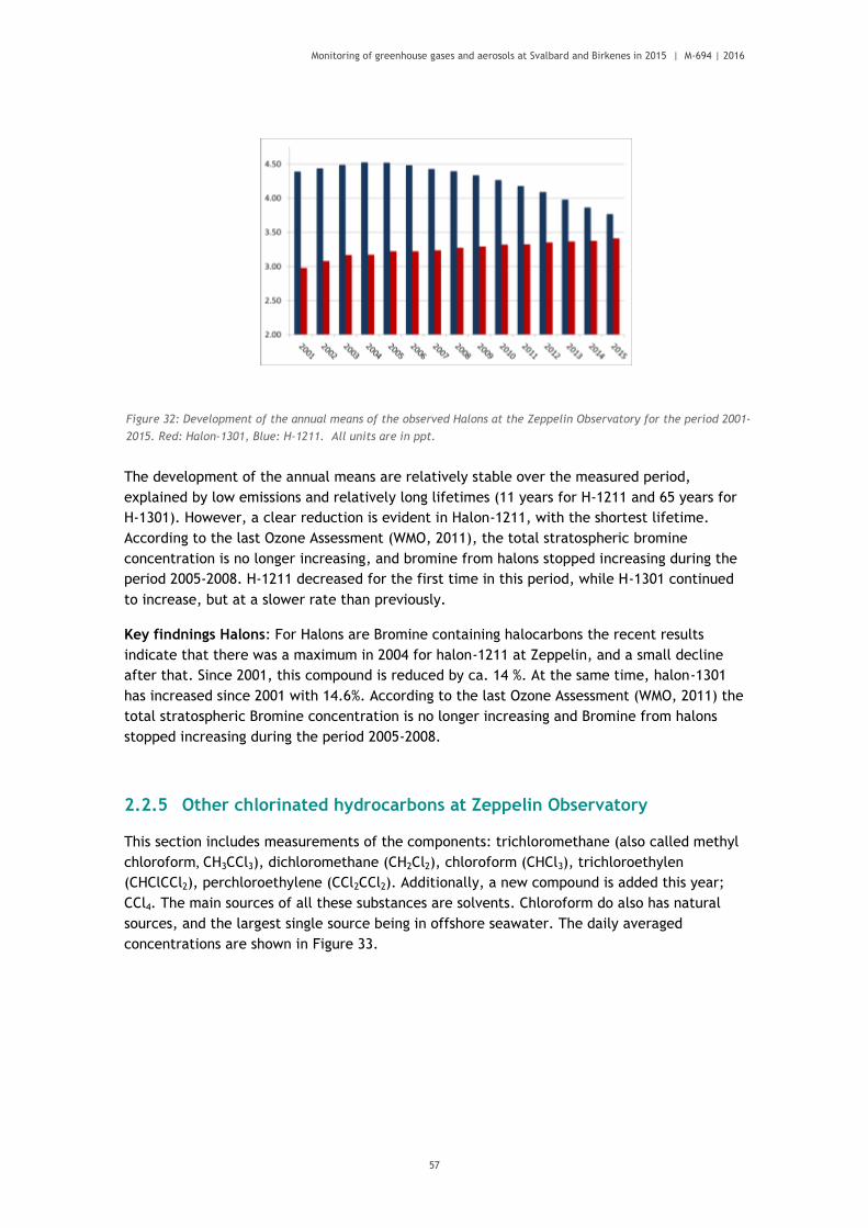
Monitoring of greenhouse gases and aerosols at Svalbard and Birkenes in 2015 | M-694 | 2016
57
Figure 32: Development of the annual means of the observed Halons at the Zeppelin Observatory for the period 2001-
2015. Red: Halon-1301, Blue: H-1211. All units are in ppt.
The development of the annual means are relatively stable over the measured period,
explained by low emissions and relatively long lifetimes (11 years for H-1211 and 65 years for
H-1301). However, a clear reduction is evident in Halon-1211, with the shortest lifetime.
According to the last Ozone Assessment (WMO, 2011), the total stratospheric bromine
concentration is no longer increasing, and bromine from halons stopped increasing during the
period 2005-2008. H-1211 decreased for the first time in this period, while H-1301 continued
to increase, but at a slower rate than previously.
Key findnings Halons: For Halons are Bromine containing halocarbons the recent results
indicate that there was a maximum in 2004 for halon-1211 at Zeppelin, and a small decline
after that. Since 2001, this compound is reduced by ca. 14 %. At the same time, halon-1301
has increased since 2001 with 14.6%. According to the last Ozone Assessment (WMO, 2011) the
total stratospheric Bromine concentration is no longer increasing and Bromine from halons
stopped increasing during the period 2005-2008.
2.2.5 Other chlorinated hydrocarbons at Zeppelin Observatory
This section includes measurements of the components: trichloromethane (also called methyl
chloroform, CH3CCl3), dichloromethane (CH2Cl2), chloroform (CHCl3), trichloroethylen
(CHClCCl2), perchloroethylene (CCl2CCl2). Additionally, a new compound is added this year;
CCl4. The main sources of all these substances are solvents. Chloroform do also has natural
sources, and the largest single source being in offshore seawater. The daily averaged
concentrations are shown in Figure 33.

Monitoring of greenhouse gases and aerosols at Svalbard and Birkenes in 2015 | M-694 | 2016
58
Figure 33: Daily average concentrations chlorinated hydrocarbons: From the upper panel: perchloroethylene (dark
blue) methylchloroform (red), trichloroethylen (green), chloroform (light blue) and dichloromethane (pink) for the
period 2001-2015 at the Zeppelin observatory. The solid lines are the empirical modelled background mixing ratio.
Methylchloroform (CH3CCl3) has continued to decrease, and accounted only for 1% of the total
tropospheric chlorine in 2008, a reduction from a mean contribution of 10% in the 1980s
(WMO, 2011). Globally averaged surface mixing ratios were around 10.5 ppt in 2008 (WMO,
2011) versus 22 ppt in 2004 (WMO, 2011). The measurements at Zeppelin show that the
component has further decreased to 3.2 ppt, a reduction of more than 90% since the
measurement start in 2001 and now contribute negligible to the atmospheric chlorine burden.
The measurements of methyl tetrachloride (CCl4) is shown in Figure 34.
2001
2002
2003
2004
2005
2006
2007
2008
2009
2010
2011
2012
2013
2014
2015
2016
25
50
75
10
15
200.0
2.5
5.0
0
20
400
5
10
15
Dichloromethane (CH2Cl
2)
pp
t v
Year
Chloroform (CHCl3)
pp
t v
Trichloroethylen (CHClCCl2),
pp
t v
Methylchloroform (CH3CCl
3)
p
pt v
Perchloroethylene (CCl2CCl
2)
pp
t v

Monitoring of greenhouse gases and aerosols at Svalbard and Birkenes in 2015 | M-694 | 2016
59
Figure 34: Daily average concentrations of carbon tetrachloride, CCl4, measured at Zeppelin Observatory. The solid
lines are the empirical modelled background mixing ratio.
It is worth noting the strong recent increase in dichloromethane (violet), and chloroform
(light blue), and the relaxation the last few years. Dichloromethane, has a lifetime of less
than 6 months, and respond rapidly to emissions changes, and about 90 % has industrial origin.
Its main applications include use in paint strippers, degreasers and solvents; in foam
production and blowing applications; and as an agricultural fumigant (WMO et al., 2011). The
most recent estimation for its natural components suggests it is comprised of a 10% combined
biomass burning and marine source. At Zeppelin, the increase since 2001 is about 76%. The
concentration is currently 54.1 ppt, a slight decrease since 2014. Strong seasonal variations
are observed for chloroform (light blue) due to a relatively short lifetime of 1 year, thus the
response to emission changes are also for this compound rapid.
The annual mean value of chloroform has increased with as much as 27% since 2005 at
Zeppelin, this is also observed at other sites (e.g. Mauna Loa at Hawaii and Barrow in Alaska).
From known emissions of this compound this increase is not expected, and the reason for this
increase is not yet clear, it might also be related to natural sources. The concentration of
trichloroethylene is very low and the annual variability is quite high, this may partly be due to
uncertainty in the measurements and missing data
01.01.2010 01.01.2012 01.01.2014 01.01.2016
75
76
77
78
79
80
81
82
83
84
85
86
87
88
89
90
CCl4

Monitoring of greenhouse gases and aerosols at Svalbard and Birkenes in 2015 | M-694 | 2016
60
Key findidngs Other Chlorinated greenhouse gases, including Methylchloride and
Methylbromide (section 2.1.6and 2.1.7) : The following five chlorinated gases are measured
at the Zeppelin Observatory: methylchloride (CH3Cl), dichloromethane (CH2Cl2), chloroform
(CHCl3), trichloromethane (CHClCCl3), methylchloroform (CH3CCl3), perchloroethylene
(CCl2CCl2). Three of these gases have increased the last years and a considerable increase in
chloroform is evident at Zeppelin of 180% compared to 2001. The reason for this is unclear.
Methylchloroform shows a decrease, and the concentrations are now very low.
Methylchloride and Methylbromide at Zeppelin are also reduced as a direct result of the
Montreal protocol.
Figure 35: Annual means of the chlorinated hydrocarbons. From upper panel: perchloroethylene (grey),
trichloromethane (red), mid panels; trichloroethylen (green), chloroform (light blue) and lower panel
dichloromethane (violet) and carbon tetrachloride (dark blue) for the period 2001-2015. All units are ppt.

Monitoring of greenhouse gases and aerosols at Svalbard and Birkenes in 2015 | M-694 | 2016
61
2.2.6 Perfluorinated (PFCs) compounds at Zeppelin Observatory
Perfluorinated compounds belong to a group of long-lived greenhouse gases, and their
contribution to the Earth’s radiative forcing has increased over the past several decades. The
impact of these highly fluorinated compounds on climate change is a concern because of their
exceptionally long atmospheric lifetimes, as well as their strong absorption in the infrared
"window" region (Baasandorj et al, 21012).
Up to 2015, the national monitoring programme only included measurements of SF6. However,
other perfluorinated compounds are also very powerful greenhouse gases with atmospheric
lifetimes as high as 50 000 years (See Table 3), and with increasing levels in the atmosphere.
NILU has from 2010 extended the monitoring of perfluorinated compounds at Zeppelin as we
have new and improved instrumentation. Several of these compounds are inclded in the
national monitoring programme from 2015, with analysis back in time until September 2010.
Hence, harmonised time series for the period September 2010-2015 is presented here for 4
new perfluorinated compounds.
2.2.6.1 Sulphurhexafluoride (SF6)
Sulphurhexafluoride, SF6. is an extremely strong greenhouse gas emitted to the atmosphere
mainly from the production of magnesium and electronics industry. Measurements of this
component has been a part of the programme since 2001. The atmospheric lifetime of this
compound is as much as 3200 years, and the global warming potential is 23500, which means
that the emission of 1 kg of this gas has a warming potential which is 23 500 times stronger
than 1 kg emitted CO2 (Myhre et al, 2013b).
The daily averaged concentration of SF6 is presented in Figure 36.
Figure 36: Daily average concentrations of SF6 for the period 2001-2015 in the left panel, and the development of the
annual mean concentrations in the right panel.
The compound is increasing with a rate of 0.27 ppt/year, and has increased as much as 70%
since the start of our measurements in 2001. The instrumentation before 2010 is not the best
suited for measurements of SF6 thus there are higher uncertainties for this compound’s mixing
2001
2002
2003
2004
2005
2006
2007
2008
2009
2010
2011
2012
2013
2014
2015
2016
4
6
8
10
SF6
pp
t v

Monitoring of greenhouse gases and aerosols at Svalbard and Birkenes in 2015 | M-694 | 2016
62
ratios than for most of the other compounds reported in the first years (see Appendix I). The
variations through the years are not due to seasonal variations, but rather to instrumental
adjustments. The improvement with the new instrumentation in 2010 is very easy to see for
this component, and the quality of the measurements has increased largely.
2.2.6.2 Perfluorocarbons or PFC’s: PFC-14, PFC-116, PFC-218, PFC-318
Perfluorocarbons or PFCs are compounds that contain only carbon and fluorine. Four of these
compounds are currently measured and reported at Zeppelin: PFC-14 (CF4) PFC-116, PFC-218,
and PFC-318. The most potent greenhouse gas is hexafluoroethane, PFC-116, which has an
atmospheric lifetime of 10 000 years and a GWP of 11 100. The gas is used as an etchant in
e.g. semiconductor manufacturing. The aluminium and the semiconductor manufacturing
industries are the major emitters of PFC-116. Octafluoropropane, PFC-218, which has an
atmospheric lifetime of 2600 years and a GWP of 8900, is also used in the electronics industry
as a plasma etching material. In medicine, PFC-218 microbubbles reflect sound waves well
and is used to improve the ultrasound signal backscatter. Octafluorocyclobutane, PFC-318,
with a life time of 3200 years and a GWP of 9540, is the third most abundant PFC in the
atmosphere (Oram et al, 2012). Although a number of potential sources of PFC-318 have been
reported, including the electronics and semi-conductor industries, there remains a large
discrepancy in the atmospheric budget. Tetrafluoromethane (CF4) PFC-14, is the most
persistent greenhouse gas of these compounds with an atmospheric lifetime of 50 000 years
and a greenhouse warming potential of 6630. It is used as a low temperature refrigerant, in
electronics microfabrication, and in neutron detectors.
The daily averaged concentrations of these compounds are shown in Figure 37.

Monitoring of greenhouse gases and aerosols at Svalbard and Birkenes in 2015 | M-694 | 2016
63
Figure 37: Daily average concentrations perfluorocarbons: From the upper panel: PFC-14 (dark blue) PFC-116 (red),
PFC-218 (green), PFC-316 (light blue) for the period 2010-2015 at the Zeppelin observatory. PFC-14 is only ranging
back to autumn 2014. The solid lines are the empirical modelled background mixing ratio.
The development of the annual means of these compounds are shown in Figure 38 are
relatively stable over the measured period, with a slight increase. It is important to note the
very low concentrations. However, PFC-14 has considerably higher concentration with an
annual mean of 80.06 ppt in 2015. With a lifetime of 50 000 years, and GWP of 6630 this is a
particularly important compound to follow.
2010
2011
2012
2013
2014
2015
2016
1.0
1.2
1.4
1.6
1.8
2.0
0.6
0.8
4.2
4.4
4.6
4.8
5.0
81.5
82.0
82.5
83.0
PFC-318
pp
t v
Year
PFC-218
pp
t v
PFC-116
pp
t v
PFC-14
pp
t v

Monitoring of greenhouse gases and aerosols at Svalbard and Birkenes in 2015 | M-694 | 2016
64
Figure 38: Annual mean concentrations perfluorocarbons hydrocarbons: PFC-116 (red), PFC-218 (green), PFC-316
(light blue) for the period 2010-2015 at the Zeppelin observatory. PFC-14 is only ranging back to autumn 2014.
The solid lines are the empirical modelled background mixing ratio.
No valid annual mean are available for 2014 for this as there were only measurements the last
months, the same apply to the other PFCs in 2010.
Nitrogen trifluoride, NF3, has a lifetime of 500 years and a GWP as high as 16100, meaning
that it is an extremely strong greenhouse gas. It is e.g. used in the manufacturing of new
generation solar panels, flat-screen televisions, touch-sensitive screens, and electronic
processors. The use of NF3 has widely increased in the past because of the rising demand in
flat-screen televisions and microelectronics. The instrument at Zeppelin we re-build and
optimized 2015 and 2016 to also provide measurements of this compounds. This will be
included in the report in 2017.
Key findings SF6 and PFC-14, PFC-116, PFC-218, PFC-318: Generally, these are extremely
potent greenhouse gas, but their concentrations are still low. The measurements show that
the concentration of SF6 has increased as much as 70% since 2001. The PFCs are new and
reported for first time this year, and they show a weak or no change since 2014.
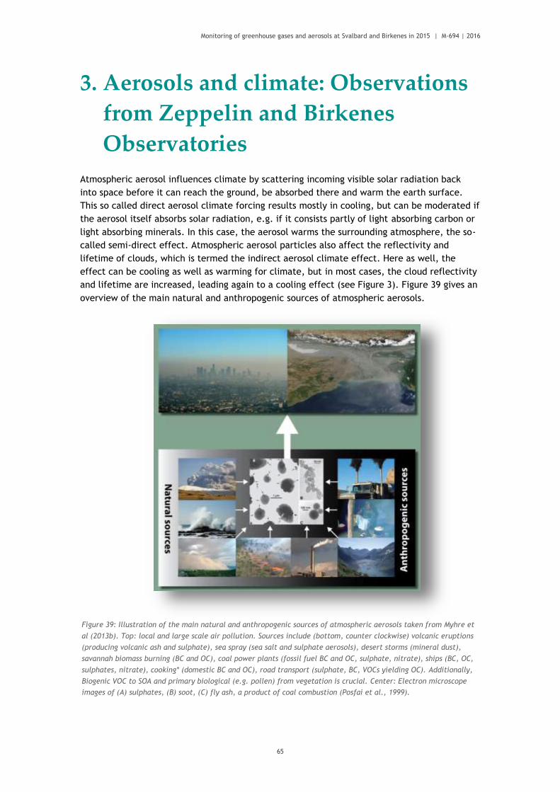
Monitoring of greenhouse gases and aerosols at Svalbard and Birkenes in 2015 | M-694 | 2016
65
3. Aerosols and climate: Observations
from Zeppelin and Birkenes
Observatories
Atmospheric aerosol influences climate by scattering incoming visible solar radiation back
into space before it can reach the ground, be absorbed there and warm the earth surface.
This so called direct aerosol climate forcing results mostly in cooling, but can be moderated if
the aerosol itself absorbs solar radiation, e.g. if it consists partly of light absorbing carbon or
light absorbing minerals. In this case, the aerosol warms the surrounding atmosphere, the so-
called semi-direct effect. Atmospheric aerosol particles also affect the reflectivity and
lifetime of clouds, which is termed the indirect aerosol climate effect. Here as well, the
effect can be cooling as well as warming for climate, but in most cases, the cloud reflectivity
and lifetime are increased, leading again to a cooling effect (see Figure 3). Figure 39 gives an
overview of the main natural and anthropogenic sources of atmospheric aerosols.
Figure 39: Illustration of the main natural and anthropogenic sources of atmospheric aerosols taken from Myhre et
al (2013b). Top: local and large scale air pollution. Sources include (bottom, counter clockwise) volcanic eruptions
(producing volcanic ash and sulphate), sea spray (sea salt and sulphate aerosols), desert storms (mineral dust),
savannah biomass burning (BC and OC), coal power plants (fossil fuel BC and OC, sulphate, nitrate), ships (BC, OC,
sulphates, nitrate), cooking* (domestic BC and OC), road transport (sulphate, BC, VOCs yielding OC). Additionally,
Biogenic VOC to SOA and primary biological (e.g. pollen) from vegetation is crucial. Center: Electron microscope
images of (A) sulphates, (B) soot, (C) fly ash, a product of coal combustion (Posfai et al., 1999).

Monitoring of greenhouse gases and aerosols at Svalbard and Birkenes in 2015 | M-694 | 2016
66
Uncertainties in assessing aerosol climate forcing hamper the attribution of changes in the
climate system. IPCC AR5 (IPCC, 2013) has high confidence in stating that atmospheric aerosol
in the past has offset a significant fraction of greenhouse gas radiative warming, although the
magnitude is connected with uncertainty. Due to the decline of aerosol concentrations as
reported in Tørseth et al (2012), Collaud Coen et al., (2013), and Asmi et al., (2013), and
summarized in Hartmann et al, 2013) the total anthropogenic radiative forcing will be even
larger in the future.
IPCC AR5 mentions progress since AR4 concerning observations of climate relevant aerosol
properties such as particle size distribution, particle hygroscopicity, chemical composition,
mixing state, optical and cloud nucleation properties. This includes the parameters covered
by the Norwegian climate monitoring programme, and underlines the importance of these
observations. IPCC AR5 also mentions a lack of long time series on these parameters and
stresses that existing time series need to be continued for maximising their informative value.
This is the core of the EU project ACTRIS, now continued in ACTRIS-2, that NILU is highly
involved in.
Due to hosting both, the data centre of the European Monitoring and Evaluation Programme
(EMEP), ACTRIS (Aerosols, Clouds, and Trace gases Research InfraStructure Network) and the
WMO Global Atmosphere Watch (GAW) World Data Centre for Aerosol (WDCA), NILU has a
position connecting the community for measuring air quality and climate relevant
atmospheric aerosol properties with the community using this data to constrain models for
assessing and predicting the aerosol climate effects. This community is represented by the
AeroCom project, an initiative for comparing these models among each other and with
various data sources, which is hosted by the Norwegian Meteorological Institute. It is
important to highlight and mention that NILUs work in hosting the WMO GAW World Data
Centre for Aerosol, among many other synergy effects, ensures a rather efficient
dissemination of the data on atmospheric aerosol properties collected within the Norwegian
climate monitoring programme, and increases its visibility. In the reporting period, the
AeroCom Phase III project, a collaboration between the Norwegian Meteorological Institute,
NILU, and the CIENS institute CICERO, funded by the Norwegian Research Council, continued
with starting designated tasks using the results of the Norwegian programme for monitoring
climate relevant aerosol properties. The tasks involve confronting climate models in AeroCom
with data collected at atmospheric observatories such as those operated by Norway.
Compared parameters will include the aerosol particle size distribution, as well as the optical
properties scattering and absorption, in order to improve the accuracy of the climate models.
Further projects relevant in this context that started in the reporting period and where the
Norwegian atmospheric monitoring programme is involved through NILU include the above
mentioned ACTRIS-2 project, and the Environmental Research Infrastructures Providing
Shared Solutions for Science and Society (ENVRIplus) project. Among others, ACTRIS-2 will
develop a primary standard for calibrating instruments measuring aerosol absorption, one of
the properties of atmospheric black carbon, and develop quality standards for measuring the
aerosol particle size distribution in the coarse size range (Dp > 1 µm) in order to further
improve assessments of aerosol climate forcing. ENVRIplus is an umbrella project for all
geoscientific research infrastructures funded or supported by the EU. One of its objectives
will be to put data from the atmospheric, marine, tectonic, and biosphere domains into a
common context by making the data interoperable, i.e. visible in common services. The
efforts started with achieving this goal first within the atmospheric domain.

Monitoring of greenhouse gases and aerosols at Svalbard and Birkenes in 2015 | M-694 | 2016
67
NILU continues to operate 3 observatories measuring aerosol properties relevant for
quantifying the direct and indirect aerosol climate effects: 1) Zeppelin Mountain / Ny Ålesund
(in collaboration with the Norwegian Polar Institute and Stockholm University); 2) Birkenes
Atmospheric Observatory, Aust-Agder, Southern Norway; 3) Troll Atmospheric Observatory,
Antarctica (observatory operated by NILU, main station operated by Norwegian Polar
Institute). The station locations represent the focal areas of the polar regions, which are
more vulnerable to climate change, as well as the regions where the largest fraction of the
Norwegian population lives. Recent developments at these stations include:
1. Zeppelin Mountain: Within the Swedish - Norwegian co-operation operating the
atmospheric observatory on Zeppelin mountain, Stockholm University maintains a set
of instruments measuring the fine-range (Dp < 1 µm) particle number size distribution,
as well as the aerosol particle scattering and absorption coefficients. Stockholm
University has had problems with timely delivery of data due to funding limitations on
the Swedish side. Beginning in 2015, these issues should have been resolved due to
additional funding from the Norwegian side covering the Swedish rental of the lab
facilities at the station. Unfortunately, data delivery by Stockholm University is still
delayed. The last data reported for the Swedish instruments at Zeppelin are for the
year 2014, and the data delivery was incomplete, i.e. didn’t cover all instruments.
Through the additional Norwegian funding for Zeppelin observatory, a number of
additional measurements have been or are planned to be installed. Due to this
funding, NILU is now operating a latest generation aethalometer at Zeppelin since
June 2015. The Magee AE33 instrument is a filter absorption photometer providing the
spectral aerosol particle absorption coefficient at 7 wavelengths from the UV to the
infra-red. The instrument is designed to be less prone to systematic uncertainties
than the previous instrument generation, and complements existing observations of
that type at Zeppelin. The new instrument is due to replace a previous generation
instrument operated at Zeppelin by the Greek Demokritos Research Institute
(Athens). Both instruments are operated in collaboration between Greece and
Norway. Another instrument now operated by NILU at Zeppelin is a time-of-flight
Aerosol Chemical Speciation Monitor (ACSM-ToF) that will yield the particle chemical
speciation with high (~hourly) time resolution. Moreover, NILU installed a Mobility
Particle Size Spectrometer (MPSS) at Zeppelin that now measures the fine-range
particle number size distribution in near-real-time, with data publicly available in
NILU’s EBAS database within 1 hour of measurement. During autumn 2016, this MPSS
will be extended to also measure the particle size distribution of the fine-range non-
volatile aerosol as a proxy of the absorbing aerosol fraction.
2. Birkenes Atmospheric Observatory: In 2015, operation of the extended aerosol
instrument set at Birkenes resumed according to the quality standards of WMO GAW
and the European infrastructure project ACTRIS. These quality standards require
networked instruments to participate in inter-comparisons at the joint GAW and
ACTRIS aerosol calibration centre in Leipzig, Germany, in regular intervals. This
measure has proven to be necessary in order to ensure comparability of observations
within the network. The frequency of these inter-comparisons, once every 2-3 years,
is balanced with minimising the downtime associated with these quality assurance
measures. In 2015, instruments targeting the direct aerosol climate effect were in the
focus of inter-comparisons. Both the integrating nephelometer and the newer filter
absorption photometer, measuring the spectral aerosol particle scattering and

Monitoring of greenhouse gases and aerosols at Svalbard and Birkenes in 2015 | M-694 | 2016
68
absorption coefficients respectively, were scheduled for being inter-compared, with
satisfactory outcome in both cases. A further improvement of the Birkenes aerosol
observation programme is scheduled for late 2016 / early 2017. The station will be
equipped with a new generation filter absorption photometer measuring the particle
absorption coefficient with an extended spectral range (from ultraviolet to infrared)
as compared to before (from blue to red). The intention behind this upgrade is to
better distinguish sources of absorbing aerosol between fossil and biomass
combustion, which are supposed to have different spectral absorption signatures in
the extended wavelength range.
3. Troll Atmospheric Observatory: Work around Troll Atmospheric Observatory
continued to follow up on a 2014 publication (Fiebig et al., 2014) funded by a base
funding project controlled by the Norwegian Research Council (Strategisk
Instituttsatsing, SIS). The article investigates the annual cycle of the baseline aerosol
at Troll as observed in the particle number size distribution and aerosol scattering
coefficient data collected at Troll. It is shown that the baseline aerosol annual cycles
in both parameters have the same physical origin. A comparison with data collected
at the Antarctic stations South pole and Dome C, yields that the baseline air annual
cycle observed at Troll is common to the whole Central Antarctic plateau. Following
the Troll baseline air masses backwards with the Lagrangian transport model
FLEXPART, the article demonstrates that these air masses descend over Antarctica
after being transported in the free troposphere and lower stratosphere from mid-
latitudes (there uplifted in fronts) or from the inter tropical convergence zone
(uplifted by convection). The article shows further that the aerosol particles
contained in Antarctic baseline air are formed in situ by photochemical oxidation of
precursor substances. A project following up on the discussed previous findings was
applied for and approved by the NFR Norwegian Antarctic Research Expeditions
(NARE) programme. Among others, the project investigates the Antarctic background
aerosol further by collecting an ultra-long exposure filter sample for chemical analysis
despite the low concentrations, and use the cluster analysis method developed with
Birkenes to identify the source regions and aerosol types found at Troll. This work is
intended to further improve our knowledge about the aerosol and aerosol processes in
pristine regions of the globe, which are often used as proxy for pre-industrial aerosol.
Uncertainty about the climate effect of pre-industrial aerosol is still one of the main
sources of uncertainty in climate predictions (Carslaw et al., 2013).

Monitoring of greenhouse gases and aerosols at Svalbard and Birkenes in 2015 | M-694 | 2016
69
An overview of all aerosol parameters currently measured at the 3 observatories can be found
in Table 4. Parameters where observations are funded by Miljødirektoratet (and which are
covered in this report) are written in green type.
Table 4: Aerosol observations at Zeppelin, Birkenes and Troll Observatory following the GAW recommendations.
Parameters in green are funded by the Norwegian Environment Agency and included in this report.
Zeppelin/Ny-Ålesund Birkenes Troll
Particle Number Size
Distribution (fundamental
to all aerosol processes)
fine mode (0.01 µm < Dp <
0.8 µm), NILU and in colla-
boration with Stockholm
University
fine and coarse mode
(0.01 µm < Dp < 10 µm)
fine mode (0.03 µm < Dp <
0.8 µm)
Aerosol Scattering
Coefficient
(addressing direct climate
effect)
spectral at 450, 550,
700 nm, in collaboration
with Stockholm University
spectral at 450, 550,
700 nm
spectral at 450, 550, 700
nm
Aerosol Absorption
Coefficient
(addressing direct climate
effect)
single wavelength at 525
nm, (Stockholm University);
single wavelength at 670 nm
(Stockholm University); 7-
wavelength (Demokritos
Athens); 7-wavelength
(NILU)
single wavelength (525 nm)
and spectral at 3
wavelengths
single wavelength at 525 nm
and spectral at 3
wavelengths.
Aerosol Optical Depth
(addressing direct climate
effect)
spectral at 368, 412, 500,
862 nm in collaboration
with WORCC
spectral at 340, 380, 440,
500, 675, 870, 1020,
1640 nm, in collaboration
with Univ. Valladolid
spectral at 368, 412, 500,
862 nm
Aerosol Chemical
Composition (addressing
direct + indirect climate
effect)
main components (ion chro-
matography), heavy metals
(inductively-coupled-plasma
mass-spectrometry)
main components (daily
resolution, offline filter-
based, ion chromatogra-
phy), heavy metals
(inductively-coupled-plasma
mass-spectrometry)
main components (ion chro-
matography), discontinued
from 2011 due to local
contamination.
Aerosol Chemical
Speciation (direct +
indirect climate effect,
source attribution,
transport)
Particle main chemical
species (hourly resolution,
online mass spectrometry)
Particle main chemical
species (hourly resolution,
online mass spectrometry)
---
Particle Mass
Concentration
--- PM2.5, PM10 PM10, discontinued from
2011 due to local
contamination
Cloud Condensation Nuclei
(addressing indirect
climate effect)
size integrated number
concentration at variable
supersaturation in
collaboration with Korean
Polar Research Institute
Size integrated number
concentration at variable
supersaturation
---

Monitoring of greenhouse gases and aerosols at Svalbard and Birkenes in 2015 | M-694 | 2016
70
3.1 Physical and optical aerosol properties at
Birkenes Observatory 3.1.1 Optical Aerosol Properties Measured In Situ at the Surface
The comprehensive set of instruments observing optical aerosol properties, i.e. those
describing the direct effect of aerosol on climate, in situ and close to the surface at Birkenes
has now been in operation for over 6 years. Figure 40 summarises the essence of these
observations for the years 2010 – 2015 in time series of the observations themselves and
relevant directly derived parameters. All properties are measured for particles with
aerodynamic diameter Dp,aero < 10 µm and at relative humidity below 40%, thus avoiding water
uptake by the aerosol particles, for best comparability between stations in the network. This
protocol follows the recommendations of the WMO GAW aerosol network, and is identical
with the recommendations of the relevant European networks (EUSAAR, ACTRIS).
Panel a) of Figure 40 displays the time series of the spectral scattering coefficient σsp at 450,
550, and 700 nm wavelength, covering the visible spectral range. Thin lines represent daily
average values for the respective wavelength, whereas the heavy green line represents the
running 8-week median for easier visibility of seasonal averages (green wavelength at 550 nm
only for clarity). The σsp time series exhibits significant variability on the time scale of days,
illustrating that particle load in an air mass varies significantly with air mass type and thus air
mass origin, i.e. with the synoptic weather situation on a time scale of 1 – 3 days. When
focussing on the graph of the running median, a slight seasonal variation can be detected,
with values higher in summer than winter.
For spectral optical aerosol properties, information is contained not only in the absolute level
of values, but also in the values at different wavelengths relative to each other. This
information is often hidden in graphs due to rapid variations of the absolute values. In order
to make this spectral information more readily accessible, the Ångström coefficient has been
defined, that can be calculated for all optical aerosol properties. Higher values of åsp
correlate with higher concentration ratios of particle surface in the fine size range (Dp <
1 µm) as compared to the coarse size range (Dp > 1 µm). Moreover, the relative size of
particles determining an optical aerosol property decreases with wavelength, i.e. smaller
wavelengths “look at” smaller particles in relative terms, larger wavelengths “look at” larger
particles. Already with these simple qualitative rules, many features exhibited by spectral
aerosol optical property data in general and Ångström coefficient data in particular can be
interpreted meaningfully.
Panel b) of Figure 40 shows the time series of the scattering Ångström coefficient åsp,
calculated from σsp(λ), again as daily averages (thin line) and running 8-week median (heavy
line). As with σsp, the strongest variability is associated to a time scale of 1-3 days, indicative
of changes associated with air mass type, origin, and synoptic weather situation. Looking at
the running median however, the seasonal cycle is more pronounced for åsp as for σsp, with åsp
values around 1.1 in winter and 1.8 in summer. As explained above, this indicates a stronger
contribution of smaller particles, i.e. particles with Dp smaller than about 120 nm, to σsp in
summer than in winter. This is consistent with number concentrations of particles in this size
range exhibiting a similar seasonal cycle, as will be discussed below. The time series of σsp
and åsp don’t show any visible underlying trend, which is consistent with the findings for other

Monitoring of greenhouse gases and aerosols at Svalbard and Birkenes in 2015 | M-694 | 2016
71
European continental background stations at Jungfraujoch (Switzerland, mountain top),
Hohenpeissenberg (Southern Germany, elevated boundary layer), and Pallas (Northern
Finland, boreal background) (Collaud Coen et al., 2013). Also the range of σsp values
encountered, 3 - 50 Mm-1 with an annual average of about 12.5 Mm-1, is consistent with
findings at comparable stations (Delene & Ogren, 2002).
The observations of the particle absorption coefficient σap at Birkenes were upgraded in 2012.
In addition to the filter absorption photometer custom-built by Stockholm University,
measuring at only one wavelength (525 nm) since late 2009, a second instrument has been
installed. The new instrument uses the same physical principle, but measures σap at 3
wavelengths (470, 522, 660 nm) with considerable less electronic noise and significantly
better long-term stability. Panel c) of Figure 40 displays the σap time series of the older, one
wavelength filter absorption photometer, with its wavelength recalculated to the same green

Monitoring of greenhouse gases and aerosols at Svalbard and Birkenes in 2015 | M-694 | 2016
72
wavelength as observed by the nephelometer (550 nm), thin line daily averages, heavy line
running 8-week median. The plot also displays the σap running median time series observed by
Figure 40: Time series of aerosol particle optical property daily means measured for 2010 - 2015 at Birkenes. Panel a) shows
the aerosol scattering coefficient σsp at 450, 550, and 700 nm wavelength measured by integrating nephelometer. Panel c)
depicts the aerosol absorption coefficient σap at 550 nm wavelength measured by filter absorption photometer, shifted from
the instrument wavelength at 525 nm to 550 nm for consistent comparison assuming an absorption Ångström coefficient of -1.
Panels b) and d) show the scattering Ångström coefficient åsp and the single scattering albedo 0 as derived properties,
respectively. Panels e) and f) display the data of the more recently installed multi-wavelength absorption photometer,
absorption coefficient σap in panel e) and absorption Ångström coefficient åap in panel f).All plots also depict the running 8-
week medians of the respective properties as heavy lines to visualize seasonal variations.
1
10
100
Aer
osol
Sin
gle
Sca
tt. A
lbed
o
0
Aer
osol
Abs
orb.
Coe
ff.
ap /
Mm
-1
Sca
tter Å
ngst
röm
Coe
ff. å
sp
Aer
osol
Sca
tt.
Coe
ff.
sp /
Mm
-1
450 nm
550 nm
700 nm
550 nm median
a)
1
2b)
450-700 nm
450-700 nm median
0.1
1
10c)
550 nm
550 nm median
550 nm new inst.
0.75
0.80
0.85
0.90
0.95
1.00
d)
550 nm
550 nm median
0.1
1
10e)
470 nm
522 nm
660 nm
470 nm median
550 nm median
660 nm median
Aer
osol
Abs
orb.
Coe
ff.
ap /
Mm
-1
01.0
1.20
10
01.0
7.20
10
01.0
1.20
11
01.0
7.20
11
01.0
1.20
12
01.0
7.20
12
01.0
1.20
13
01.0
7.20
13
01.0
1.20
14
01.0
7.20
14
01.0
1.20
15
01.0
7.20
150
2f)
470-522 nm
470-660 nm
522-660 nm
470-522 nm median
470-660 nm median
522-660 nm median
Abs
orpt
ion Å
ngst
röm
Coe
ff. å
ap
Time / Date

Monitoring of greenhouse gases and aerosols at Svalbard and Birkenes in 2015 | M-694 | 2016
73
the new filter absorption photometer (also recalculated to 550 nm wavelength) as an
indicator for the goodness of overlap between the 2 instruments measuring the same
property. Apart from the variation with synoptic transport and air mass origin, σap does not
seem to exhibit significant seasonal variation. The values of σap fall in the range of 0.3 –
4 Mm-1 with annual means around 1 Mm-1, whereas 0 varies between 0.86 – 0.96.When
comparing the median time series of old (panel c) heavy black line) and new filter absorption
photometer (panel c) red line), the very good co-variation of the two instruments measuring
the same property is rather re-confirming, especially in the begin of the comparison period.
Towards the end of the comparison period so far available, the systematic deviation of both
instruments in absolute terms is increasing. Both instruments have participated in inter-
comparison workshops at the joint calibration centre for aerosol physics for WMO GAW and
the European ACTRIS Research Infrastructure at the Institute for Tropospheric Research,
Leipzig, Germany. The older instrument’s inter-comparison dates back to 2013, the new
instrument participated in 2015. Due to late arrival of the results for the new instrument
close to the deadline for this report, it wasn’t possible yet to join the data of both
instruments into one common σap time series for Birkenes. However, judging from the known
stability properties of both instruments, experiences of other stations in the WMO GAW
network, and the increasing age of the older instrument, which was first deployed in 2006 at
the old Birkenes station, it appears likely that the observations of σap at Birkenes were
upgraded just in time.
In order to cover the largest possible time period, panel d) of Figure 40 shows the time series
of the aerosol particle single scattering albedo 0 based on the time series of the older filter
absorption photometer, again daily averages (thin line) and 8-week running median (heavy
line). When looking at the fraction of incident light interacting with the particle phase of an
aerosol, the single scattering albedo 0 quantifies the fraction of light scattered by the
particles rather than absorbed. It thus quantifies how absorbing the average aerosol particle
is and does not scale with the absolute amount of particles, with 0 values decreasing with
increasing absorption of the average particle. For a purely scattering aerosol, 0 is 1, and
decreases with increasing fraction of light absorbing components in the aerosol particle
phase. The most prominent features in the 0 time series are the pronounced annual cycle,
with lower 0 values and higher particle absorption in winter, and the underlying increasing
tendency in 0, i.e. decreasing tendency in absorption of the average particle, until 2014,
which seems to level out thereafter. The annual cycle in 0 has been discussed in previous
reports of the Birkenes aerosol dataset, and has been connected to the combustion of
biomass in wood stoves for domestic heating in the winter season. Bearing in mind the
uncertainty of a trend based on a 6-year time series, 0 has increased at Birkenes by 4.2%
over the years 2010 – 2014 disregarding the annual cycle. A tendency towards less aerosol
absoprtion has also been observed for stations in the continental U.S. and Alaska (Barrow),
but only few stations in continental Europe (Hohenpeissenberg, Germany) (Collaud Coen et
al., 2013). The underlying increasing tendency in 0 is likely connected to policy measures
oriented towards improving air quality. Over the past decades, regulations limiting the
particle emissions of motorised vehicles came into effect, and old wood stoves have been
replaced with newer ones that use secondary combustion technology to reduce emissions.
Motorised transport as well as domestic heating involve combustion processes, which are also
source of absorbing aerosol particles due to unavoidably incomplete combustion. Reduction of
these emissions has likely co-reduced emissions of absorbing particles, leading to the
observed increasing tendency in 0. As of 2014, the increasing tendency of 0 seems to level
out, but more data is needed for a conclusion on this. It is likely that the tendency towards

Monitoring of greenhouse gases and aerosols at Svalbard and Birkenes in 2015 | M-694 | 2016
74
less absorbing aerosol observed in Birkenes will decrease in the years to come, simply
because further reductions will be harder to achieve. It needs to be pointed out that firm
attributions of the reasons for both, annual cycle and tendency in 0, cannot be established
in the scope of this report. For this, advanced statistical methods such as cluster analysis and
positive matrix factorisation need to be used in connection with modelling the transport of air
masses observed at Birkenes back to their sources regions.
Panels e) and f) of Figure 40 are based on data of the new filter absorption photometer,
measuring σap spectrally at 3 wavelengths, as opposed to 1 wavelength with the older
instrument. Panel e) shows the time series of σap for all 3 wavelengths in the same way as
before (thin line daily means, heavy line running 8-week median). In the same way, panel f)
depicts the time series of the absorption Ångström coefficient åap for all 3 wavelength pairs
provided by the new instrument. Not surprisingly, the σap time series for the new filter
absorption photometer exhibits the same general features as for the old one, with the graphs
for all 3 wavelengths following each other. Changes in the relative differences between σap
values at different wavelengths are visible, but difficult to quantify in this plot. This is
facilitated by the absorption Ångström coefficient åap data displayed in panel f). For åap, the
information on relative particle size concerns not the overall aerosol particle phase, but the
fraction of absorbing particles. Thus, considering åap data allows to investigate changes in
source and transport of the absorbing particle fraction in the aerosol. When looking at the åap
data in panel f) of Figure 40, an annual cycle is apparent that is opposite of the annual cycles
seen in scattering Ångström coefficient åsp and single scattering albedo 0. Both åsp and 0
increase in summer as compared to winter, åsp because of a summer increase in small
particles due to particle formation from biogenic precursors, 0 because of fewer combustion
emissions in summer than in winter. For åap, values increase in winter as compared to
summer, indicating, in relative terms, higher abundance of smaller absorbing particles in
winter than in summer. This observation is consistent with assuming emissions from domestic
heating by wood stoves to contribute to the Birkenes winter aerosol, which is the explanation
for the decreased winter values of 0. The size of the absorbing aerosol particles increases
with aerosol age. Consequently, a smaller size of the absorbing particles indicates a younger
combustion aerosol and a closer combustion source, which is consistent with a scattered
distribution of houses using wood stoves for heating, i.e. typical for Southern Norway. The
previous instrument upgrade of aerosol absorption measurements in Birkenes has thus
provided another indication for the contribution of wood stove emissions to the Birkenes
winter aerosol. Further information can be expected from the additional upgrade extending
the spectral range of particle absorption observations scheduled for late 2016 / early 2017.
Another important puzzle piece in distinguishing sources of absorbing aerosol particles would
be the size distribution of the non-volatile particle fraction as a proxy of the size distribution
of absorbing particles. This property could be measured with a relatively simple addition to
the existing instruments at Birkenes, similar to the new instrument to be deployed by NILU at
Zeppelin.
3.1.2 Physical Aerosol Properties Measured In Situ at the Surface
Figure 41 shows the time series of the particle number size distribution (PNSD) measured at
Birkenes in 2015, separated into 4 different panels by season. In this plot type, the x-axis
holds the time of the observation, whereas the y-axis holds the particle diameter Dp on a
logarithmic scale. The logarithmic colour scale holds the particle concentration, normalised

Monitoring of greenhouse gases and aerosols at Svalbard and Birkenes in 2015 | M-694 | 2016
75
to the logarithmic size interval, dN / dlog Dp. The use of logarithmic axis is common when
displaying PNSD information since both, particle diameter and particle concentration, tend to
span several orders of magnitude while containing relevant information over the whole scale.
In this report, the PNSD reported for Birkenes covers for the first time the whole size range
between 0.01 – 10 µm by combining the information of 2 instruments, one each focussing on
the fine and coarse size ranges, into a common PNSD product (see appendix for details).
Where existing, operating procedures and quality standards defined by the WMO Global
Atmosphere Watch Programme and the European research infrastructure ACTRIS have been
used (Wiedensohler et al., 2012).
There doesn’t exist any unique connection between the PNSD and air mass type, but the PNSD
still is normally fairly characteristic for the air mass, and can serve, together with the single
scattering albedo 0, and the scattering Ångström coefficient åsp, as valuable indication of air
mass origin, which at Birkenes shifts with the synoptic weather situation. Consequently, the
information content of a PNSD time series plot is too high to be discussed in detail in this
overview-type annual report. The PNSD and 0 observations reconfirm previous findings on
the dominant air mass types at Birkenes, which consist of: 1) clean Arctic background aerosol;
2) Central and Eastern European aerosol; 3) Arctic haze; 4) biogenic aerosol, i.e. vegetation
emitted precursor gases condensing to the particle phase by photooxidation; 5) wood
combustion aerosol from domestic heating.
In order to condense the information in the PNSD time series, Figure 42 shows the time series
of selected PNSD integrals, i.e. the concentration of particles falling into selected size
intervals. The size intervals are chosen to represent characteristic processes governing the
Figure 41: 2015 time series of particle number size distribution at Birkenes, panel a) winter, panel b) spring,
panel c) summer, panel d) autumn.
dN
/ d
logD
p /cm
-3
10-2
10-1
100
101
102
103
104
a)
01.0
1.2
015
01.0
2.2
015
01.0
3.2
015
01.1
2.2
015
01.0
1.2
016
0.01
0.1
1
10
Part
icle
Dia
mete
r / µ
m
Time / Date
b)
01.0
3.2
015
01.0
4.2
015
01.0
5.2
015
Time / Date
c)
01.0
6.2
015
01.0
7.2
015
01.0
8.2
015
0.01
0.1
1
10
Part
icle
Dia
mete
r / µ
m
Time / Date
d)
01.0
9.2
015
01.1
0.2
015
01.1
1.2
015
Time / Date
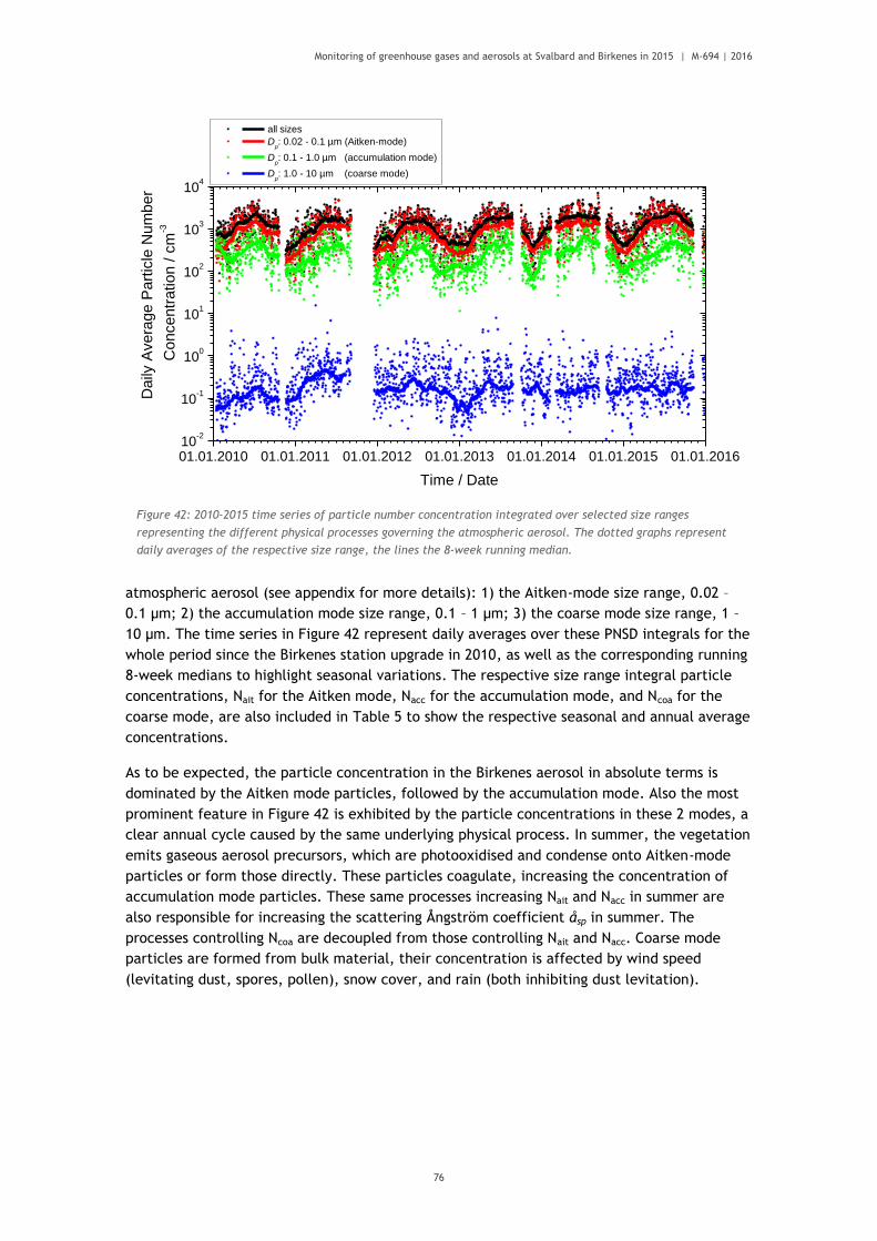
Monitoring of greenhouse gases and aerosols at Svalbard and Birkenes in 2015 | M-694 | 2016
76
atmospheric aerosol (see appendix for more details): 1) the Aitken-mode size range, 0.02 –
0.1 µm; 2) the accumulation mode size range, 0.1 – 1 µm; 3) the coarse mode size range, 1 –
10 µm. The time series in Figure 42 represent daily averages over these PNSD integrals for the
whole period since the Birkenes station upgrade in 2010, as well as the corresponding running
8-week medians to highlight seasonal variations. The respective size range integral particle
concentrations, Nait for the Aitken mode, Nacc for the accumulation mode, and Ncoa for the
coarse mode, are also included in Table 5 to show the respective seasonal and annual average
concentrations.
As to be expected, the particle concentration in the Birkenes aerosol in absolute terms is
dominated by the Aitken mode particles, followed by the accumulation mode. Also the most
prominent feature in Figure 42 is exhibited by the particle concentrations in these 2 modes, a
clear annual cycle caused by the same underlying physical process. In summer, the vegetation
emits gaseous aerosol precursors, which are photooxidised and condense onto Aitken-mode
particles or form those directly. These particles coagulate, increasing the concentration of
accumulation mode particles. These same processes increasing Nait and Nacc in summer are
also responsible for increasing the scattering Ångström coefficient åsp in summer. The
processes controlling Ncoa are decoupled from those controlling Nait and Nacc. Coarse mode
particles are formed from bulk material, their concentration is affected by wind speed
(levitating dust, spores, pollen), snow cover, and rain (both inhibiting dust levitation).
Figure 42: 2010-2015 time series of particle number concentration integrated over selected size ranges
representing the different physical processes governing the atmospheric aerosol. The dotted graphs represent
daily averages of the respective size range, the lines the 8-week running median.
01.01.2010 01.01.2011 01.01.2012 01.01.2013 01.01.2014 01.01.2015 01.01.201610
-2
10-1
100
101
102
103
104
all sizes
Dp: 0.02 - 0.1 µm (Aitken-mode)
Dp: 0.1 - 1.0 µm (accumulation mode)
Dp: 1.0 - 10 µm (coarse mode)
Daily
Avera
ge P
art
icle
Num
ber
Concentr
ation /
cm
-3
Time / Date

Monitoring of greenhouse gases and aerosols at Svalbard and Birkenes in 2015 | M-694 | 2016
77
3.1.3 Birkenes Aerosol Properties Measured In Situ at the Surface: Summary
In terms of particle concentration, the year 2015 is similar to 2014, but somewhat distinct
from the previous years. As can be seen from Table 5, the particle concentrations in Aitken
and accumulation mode Nait and Nacc are higher in winter, spring, and summer as compared to
previous years. These deviations are caused by the unusual meteorological conditions in the
reporting year, with winter temperatures falling rarely below freezing, very early onset of
spring, and high summer temperatures. These conditions caused stronger and prolonged
biogenic emissions of aerosol precursor substances, leading to the observed higher particle
concentrations on seasonal and annual average for Aitken and accumulation mode size range
Table 5: 2010 - 2015 seasonal and annual means of size distribution integrals, scattering coefficient, absorption
coefficient, and single scattering albedo.
Year Season Nait / cm-3
Nacc / cm-3
Ncoarse / cm-3
Ntotal / cm-3
σsp (550 nm) / Mm-1
σap (550 nm) / Mm-1
0 (550 nm)
2009/10 Winter 440 384 0.087 824 16.82 3.09 0.88
2010 Spring 1030 324 0.311 1354 12.33 0.78 0.93
2010 Summer 1511 488 0.323 1999 11.30 0.70 0.94
2010 Autumn 835 299 0.260 1135 7.26 0.71 0.90
2010 Whole Year
973 362 0.256 1336 11.52 1.24 0.91
2010/11 Winter 454 285 0.311 739 16.96 2.18 0.89
2011 Spring 1127 369 0.639 1496 18.67 1.26 0.93
2011 Summer 1391 438 0.572 1829 15.43 0.74 0.95
2011 Autumn 1594 464 0.966 2059 29.74 2.87 0.92
2011 Whole Year
1047 371 0.565 1418 20.26 1.69 0.93
2011/12 Winter 424 213 0.305 637 11.29 1.00 0.91
2012 Spring 1107 271 0.386 1378 15.10 0.86 0.93
2012 Summer 1314 392 0.485 1706 12.62 0.67 0.95
2012 Autumn 661 152 0.365 814 9.80 0.65 0.92
2012 Whole Year
889 263 0.375 1152 12.22 0.83 0.92
2012/13 Winter 383 183 0.183 566 12.48 0.92 0.90
2013 Spring 1190 352 0.411 1543 17.03 0.68 0.95
2013 Summer 1519 447 0.467 1967 13.81 0.56 0.96
2013 Autumn 701 162 0.417 864 8.89 0.64 0.91
2013 Whole Year
1020 304 0.391 1324 13.73 0.67 0.94
2013/14 Winter 699 333 0.347 1033 22.89 1.45 0.93
2014 Spring 1464 402 0.334 1866 12.95 1.09 0.93
2014 Summer 1723 625 0.343 2349 15.85 0.57 0.96
2014 Autumn 1122 446 0.385 1568 18.76 0.91 0.94
2014 Whole Year
1279 456 0.338 1735 16.99 0.99 0.94
2014/15 Winter 549 192 0.307 741 13.98 0.61 0.94
2015 Spring 1425 332 0.348 1757 12.72 0.68 0.94
2015 Summer 1979 559 0.395 2539 12.45 0.62 0.95
2015 Autumn 1130 422 0.257 1553 15.69 0.84 0.92
2015 Whole Year
1326 390 0.340 1717 14.36 0.67 0.94

Monitoring of greenhouse gases and aerosols at Svalbard and Birkenes in 2015 | M-694 | 2016
78
The seasonal and absolute trend in the optical aerosol properties over the years reflects
discussed in Figure 40. The average winter aerosol particles becomes less absorbing over the
years, and the differences between the average winter and summer aerosol particles in this
respect decrease.
3.1.4 Column-Integrated Optical In Situ Aerosol Properties Measured by Ground-Based Remote Sensing
Ground-based remote sensing of the optical characteristics of aerosols in the atmospheric
total column is conducted with multi-wavelength sun-photometers. A sun-photometer is
oriented towards the sun to detect the solar radiation attenuated along the slant path from
the top-of-atmosphere to the ground. The atmospheric aerosol load leads to a decrease in the
solar radiation transmitted through the atmosphere. This decrease depends on the aerosol
optical depth (AOD), which is given by the integral of the volume aerosol extinction
coefficient along the vertical path of the atmosphere. The wavelength dependence of AOD,
described by the Ångström exponent (Å) is a qualitative indicator of the particle size and
contains information about the aerosol type. The larger the Ångström exponent, the smaller
the size of the particles measured.
Photos of instruments used for monitoring of spectral resolved AOD at Birkenes and Ny-
Ålesund (see below), their main characteristics are given in Appendix II, and detailed Tables
with monthly data for all years are given in Appendix I.

Monitoring of greenhouse gases and aerosols at Svalbard and Birkenes in 2015 | M-694 | 2016
79
AOD measurements started at the Birkenes Observatory in spring 2009, utilizing an automatic
sun and sky radiometer (CIMEL type CE-318, instrument #513). The retrieval method is that of
the AERONET version 2 direct sun algorithm (for details: http://aeronet.gsfc.nasa.gov).
Quality assured (Level 2) data are available for the seven years of operation, 2009 - 2015. The
Cimel instrument was not calibrated in 2015, but the calibration in October and November
2014 and a more recent one in summer 2016 was used for data calibration. Therefore, quality
Figure 43: 2009 - 2015 time series of aerosol optical depth (AOD) at 500 nm wavelength in the atmospheric
column above Birkenes (upper panel) and Ångström coefficient describing the AOD wavelength dependence (lower
panel). Mean values and standard deviations are given.

Monitoring of greenhouse gases and aerosols at Svalbard and Birkenes in 2015 | M-694 | 2016
80
assured AERONET level 2 data are available for the whole period when solar elevation allows
reasonable data, in 2015 from March to November.
The AOD and Ångström coefficient time series and seasonal variations are shown Figure 43
and Figure 44. The 2015 monthly mean and mean values for all years are shown in Table 6.
Data for all years are given in Appendix I. There are no obvious trends visible in the seven
years of observations. Data gaps are caused by lack of sun light hours during the winter
months (from last part of November through first part of February). In general, AOD measured
at Birkenes are relatively low, compared to central European observations. E.g., AERONET
climatological values for Cabauw, the Netherlands, vary between 1.2 ± 0.06 in December and
3.1 ±0.19 in April). In 2015, AOD values at Birkenes were very low, even compared to previous
Figure 44: Monthly mean aerosol optical depth (AOD) at 500 nm wavelength in the atmospheric column above
Birkenes (upper panel) and Ångström coefficient describing the AOD wavelength dependence (lower panel). Mean
values and standard deviations are given.

Monitoring of greenhouse gases and aerosols at Svalbard and Birkenes in 2015 | M-694 | 2016
81
years at this station. The highest monthly average AOD of 0.096 was observed in July, while
monthly means in March and throughout autumn were 0.04 or even lower. The largest spreads
of daily values within a month were observed in July and August (standard deviations of 0.67
and 0.61, respectively). In these months, a small number daily mean AOD values of more than
0.15 were recorded, and on one day in July (day 193) even values of up to 0.7 were measured
(which were discarded due to too few single values to calculate a daily means. AOD values for
2015 are at the lower end of the spread observed during the years 2009 – 2014, comparable to
observations in 2012. All monthly means are smaller than the multi-year average. The low-
AOD period with values of 0.04 or less in autumn 2015 is the longest observed since the start
of observations at Birkenes.
Ångström exponent monthly means are close to the long-term means observed at Birkenes
and also follows the seasonal variation of previous years, with monthly means close to 1.0 in
the first half of the year, maximum values close to 1.5 in late summer and decreasing values
again in autumn. All 2015 monthly means are within the standard deviations of all years at
the station.
Table 6: Monthly mean values for 2014 and mean for the time period 2009-2014, plus standard deviations, for
aerosol optical depth (AOD) and Ångström coefficient observed in Birkenes. In addition, the number of days with
cloud free and quality assured observations are given.
Month/Year Jan Feb Mar Apr May Jun Jul Aug Sep Oct Nov
Aerosol optical depth (AOD)
2015 0.04
±0.02
0.07
±0.02
0.07
±0.03
0.06
±0.02
0.10
±0.07
0.09
±0.06
0.04
±0.02
0.03
±0.03
0.04
±0.01
Mean
09-15
0.02
0.01
0.03
±0.01
0.08
±0.06
0.11
±0.07
0.10
±0.04
0.08
±0.04
0.13
±0.07
0.11
±0.06
0.08
±0.03
0.06
±0.03
0.04
±0.01
Ångström coefficient (Å)
2015 0.93
± 0.16
1.06
± 0.13
1.11
± 0.20
1.30
± 0.20
1.49
± 0.20
1.37
±0.26
1.30
±0.23
1.23
±0.25
0.84
±0.33
Mean
09-15
0.96
±0.14
1.04
±0.05
0.97
±0.35
1.21
±0.29
1.23
±0.25
1.38
±0.20
1.46
±0.28
1.35
±0.23
1.12
±0.22
1.16
±0.27
0.97
±0.28
Number of days with cloud-free and quality assured observations (AERONET level 2)
2015 6 1 14 21 21 16 9 11 3
Total
09-15 7 2 49 54 93 114 127 107 68 52 11

Monitoring of greenhouse gases and aerosols at Svalbard and Birkenes in 2015 | M-694 | 2016
82
3.2 Physical and optical aerosol properties at
Zeppelin Observatory 3.2.1 Aerosol Properties Measured In Situ at the Surface at Zeppelin
Observatory
Figure 45 summarises the first few months of spectral aerosol particle absorption coefficient
σap data collected at Zeppelin Observatory since deployment of the new aethalometer in June
2015. The top panel displays daily averaged data for all 7 wavelengths (thin lines), as well as
running 8-week medians (heavy lines), here only for 3 wavelengths to improve readability of
the graph. The middle panel shows graphs of the absorption Ångström coefficient åap for 3
wavelength pairs representing short wave end, long wave end, and full range of the measured
wavelength spectrum. The åap data are plotted as 8-week median only since daily averages
Figure 45: Time series graphs of the first months of data collected by the new filter absorption photometer at
Zeppelin Observatory since deployment in June 2015. Top: daily means of absorption coefficient at all 7 measured
wavelengths (thin lines), and 8-week running medians for top, middle and bottom of observed spectral range (heavy
lines). Middle: 8-month running medians of absorption Ångström coefficient, top, bottom, and whole observed
spectral range. Bottom: fraction of biomass burning aerosol contributing to particle absorptionas calculated by
instrument, together with ID number of filter spot.
0.01
0.1
1
10
Ae
roso
l A
bso
rption
Co
eff.
ap / M
m-1
370 nm
470 nm
525 nm
590 nm
660 nm
880 nm
950 nm
370 nm median
590 nm median
950 nm median
0
1
370/470 nm median
880/950 nm median
370/950 nm median
Ab
so
rbtion
Ån
gstr
öm
Co
effic
ien
t
0
20
40
BB fraction
Filter spot
number
Bio
ma
ss B
urn
ing
Fra
ction
/ %
01.05.2015 01.08.2015 01.11.2015
120
140
160
180
550 nm
Time / Date
Filte
r Sp
ot N
um
be
r

Monitoring of greenhouse gases and aerosols at Svalbard and Birkenes in 2015 | M-694 | 2016
83
are too noisy due to the low particle load commonly observed at Zeppelin. The bottom panel
of Figure 45 depicts the fraction of biomass burning aerosol contributing to the sampled
aerosol as calculated by the instrument. To calculate the biomass burning fraction, the
instrument uses the different spectral absorption characteristics of aerosol from fossil as
compared to biofuel combustion (Sandradewi et al., 2008). When interpreting this parameter,
caution needs to be exercised. The assumed absorption models for fossil and biofuel
combustion emissions have been derived for conditions in rural Switzerland. These conditions
are certainly not representative for Arctic aerosol. However, if interpreted in a qualitative
way, the parameter may give a first indication of changes in the properties of the absorbing
aerosol particle fraction.
Even though the time series of the aethalometer at Zeppelin spans only half a year at this
point, a few interesting features can be detected already now. The time series of σap (top
panel of Figure 45) exhibits the same annual cycle as described already in the data of the
aethalometer instrument collected in earlier years (Eleftheriadis et al., 2009), with lower
values in summer and higher ones in winter. These variations have been attributed to changes
in combustion aerosol source strength caused by emissions from domestic heating in the
relevant source regions, e.g. Northern and Central Russia (Law & Stohl, 2007). This pattern is
moderated by incidents of emissions from big forest fires reaching the Arctic, which can
increase aerosol particle absorption in episodes also in summer (e.g. Stohl et al., 2007). This
pattern is mirrored in the time series of the biomass burning fraction calculated by the
MAGEE AE33 instrument, which increases for episodes summer and towards winter. However,
obvious artefacts can be detected in the calculation of the biomass burning fraction, which
increases also with aerosol loading on the filter, and drops when the filter spot is changed
(see filter spot number also plotted in bottom panel of Figure 45).
Probably most interesting in the data provided by the new filter absorption photometer is the
aerosol absorption Ångström coefficient åap, which seems to display its own annual cycle.
Towards autumn, åap increases in the ultraviolet (UV) range, and decreases in the infrared (IR)
range. In descriptive terms, this means that the absorbing aerosol fraction in autumn
decreases in particle size as seen by UV light (which weighs smaller particles more), and
increases in particle size as seen by IR light (which weighs larger particles more). An
explanation of this puzzling phenomenon needs to await further measurements at Zeppelin.
Also funded by the extraordinary grant of the Norwegian Ministry of Climate and Environment,
an instrument observing the size distribution of the non-volatile particle fraction as a proxy of
the absorbing particle fraction will be installed at Zeppelin by NILU in autumn 2016.
3.2.2 Column-Integrated Optical In Situ Aerosol Properties Measured by Ground-Based Remote Sensing at Ny-Ålesund
In 2002, Physikalisch-Meteorologisches Observatorium Davos/World Radiation Center
(PMOD/WRC) in collaboration with NILU, started AOD observations in Ny-Ålesund (at the
Sverdrup station, 46 m a.s.l.) as part of the global AOD network on behalf of the WMO GAW
program. A precision filter radiometer (PFR) measures the extinction in four narrow spectral
bands at 368 nm, 415 nm, 500 nm and 862 nm. Data quality control includes instrumental
control like detector temperature and solar pointing control as well as objective cloud
screening. Ångström coefficients are derived for each set of measurements using all four PFR

Monitoring of greenhouse gases and aerosols at Svalbard and Birkenes in 2015 | M-694 | 2016
84
channels. Calibration is performed annually at PMOD/WRC. Quality assured data are available
at the World Data Center of Aerosols (WDCA), hosted at NILU (see https://ebas.nilu.no).
In Ny-Ålesund, the solar elevation is less than 5° before 4 March and after 10 October,
limiting the period with suitable sun-photometer observations to the spring-summer-early
autumn seasons (NILU contributes to a Lunar Arctic initiative to fill the gap in the wintertime
AOD climatology by using Lunar photometer, see Appendix II). In 2015, sun-photometer
observations started on 20 March and lasted until 18 September; reliable AOD values are
available on 76 days. The AOD and Ångström coefficients time series of monthly means and
standard deviation are shown in Figure 46, while the 2015 values on the background of the
average data and their standard deviation from the whole 14-year period are shown in Figure
47. The 2015 monthly mean values and standard deviations for all years are given in Table 7.
Data for all years are given in Appendix I.

Monitoring of greenhouse gases and aerosols at Svalbard and Birkenes in 2015 | M-694 | 2016
85
In all months except July, monthly mean AOD values are equal to or smaller than the long-
term mean; in March the value is outside the standard deviation of previous years. The most
prominent feature in AOD is a short episode in July (9 – 12) with daily means of up to 0.7 and
single measurement values of up to 1.2. This period increases the monthly means to 0.15 and
the standard deviation to 0.2. A preliminary analysis of the event by Zielinski et al. concluded
that this event was due to the advection of air masses from massive forest fires in Alaska; it
will be further analysed and published in the near future. Besides comparison with other
Figure 46: 2002 - 2015 time series of aerosol optical depth (AOD) at 500.5 nm wavelength in the atmospheric
column above Ny-Ålesund (upper panel) and Ångström coefficient (lower panel). Monthly mean values and
standard deviations are given.

Monitoring of greenhouse gases and aerosols at Svalbard and Birkenes in 2015 | M-694 | 2016
86
measurements in Ny-Ålesund and Hornsund, also the Ångström exponent values from this
period confirm the validity of the measurements. Ångström coefficient monthly means were
very stable throughout almost the whole measurement period close to a value of 1.4.
However, both in April and September significantly lower values (< 1.0) were observed; the
smallest daily means of 0.25 was recorded in mid-September. Generally, in Ny-Ålesund
seasonal variation of the Ångström coefficient is very weak, and the monthly mean Ångström
coefficiens in 2015 lie within the standard deviation range of the long-term monthly means,
except September. This period with extremely low AE should be studied in more detail as
well.
Figure 47: Seasonal variation of the aerosol optical depth (AOD) (upper panel) and Ångström coefficient (lower
panel) observed in Ny-Ålesund. Values marked in grey are the mean and standard deviations for the time period
2009-2015; the 2015 monthly mean and standard deviations are shown in green.

Monitoring of greenhouse gases and aerosols at Svalbard and Birkenes in 2015 | M-694 | 2016
87
Table 7: Monthly mean values for 2014 and mean for the time period 2002-2014 for March to September, plus
standard deviations, for aerosol optical depth (AOD) and Ångström coefficient observed in Ny-Ålesund. In
addition, the number of days with cloud free and quality assured observations are given.
Month/Year Mar Apr May Jun Jul Aug Sep
Aerosol optical depth (AOD)
2015 0.05
±0.02 0.10
±0.03 0.07
±0.02 0.05
±0.01 0.15
±0.20 0.05
±0.02 0.05
±0.01
Mean 2002-2015
0.10 ±0.06
0.10 ±0.06
0.10 ±0.06
0.06 ±0.04
0.07 ±0.03
0.06 ±0.03
0.06 ±0.03
Ångström coefficient (Å)
2015 1.32
±0.17 1.23
±0.26 1.47
±0.14 1.50
±0.20 1.47 ±0.6
1.56 ±0.16
1.18 ±0.52
Mean 2002-2015
1.15 ±0.23
1.25 ±0.26
1.36 ±0.26
1.46 ±0.23
1.43 ±0.22
1.39 ±0.31
1.37 ±0.32
Number of days with cloud-free and quality assured observations
2015 5 17 15 9 17 13 6
Total 2002-2015
61 160 153 145 167 125 111

Monitoring of greenhouse gases and aerosols at Svalbard and Birkenes in 2015 | M-694 | 2016
88
4. References
Aas, W., Platt, S., Solberg, S., Yttri, K.E. (2016) Monitoring of long-range transported air
pollutants in Norway, annual report 2015. Kjeller, NILU (Miljødirektoratet rapport, M-
562/2016) (NILU OR, 13/2016).
Asmi, A., Collaud Coen, M., Ogren, J. A., Andrews, E., Sheridan, P., Jefferson, A.,
Weingartner, E., Baltensperger, U., Bukowiecki, N., Lihavainen, H., Kivekäs, N., Asmi, E.,
Aalto, P. P., Kulmala, M., Wiedensohler, A., Birmili, W., Hamed, A., O'Dowd, C., G
Jennings, S., Weller, R., Flentje, H., Fjaeraa, A. M., Fiebig, M., Myhre, C.E.L., Hallar, A.
G., Swietlicki, E., Kristensson, A., Laj, P. (2013) Aerosol decadal trends - Part 2: In-situ
aerosol particle number concentrations at GAW and ACTRIS stations. Atmos. Chem. Phys.,
13, 895-916. doi:10.5194/acp-13-895-2013.
Baasandorj, M., Hall, B. D., Burkholder, J. B. (2012) Rate coefficients for the reaction of
O(1D) with the atmospherically long-lived greenhouse gases NF3, SF5CF3, CHF3, C2F6, c-
C4F8, n-C5F12, and n-C6F14. Atmos. Chem. Phys., 12, 11753-11764. doi:10.5194/acp-12-
11753-2012.
Coen, M.C., Andrews, E., Asmi, A., Baltensperger, U., Bukowiecki, N., Day, D., Fiebig, M.,
Fjaeraa, A. M., Flentje, H., Hyvärinen, A., Jefferson, A., Jennings, S. G., Kouvarakis, G.,
Lihavainen, H., Myhre, C.E.L, Malm, W. C., Mihapopoulos, N., Molenar, J. V., O'Dowd, C.,
Ogren, J. A., Schichtel, B. A., Sheridan, P., Virkkula, A., Weingartner, E., Weller, R., Laj,
P. (2013) Aerosol decadal trends - Part 1: In-situ optical measurements at GAW and
IMPROVE stations. Atmos. Chem. Phys., 13, 869-894. doi:10.5194/acp-13-869-2013.
Dalsøren, S. B., Myhre, C.E.L., Myhre, G., Gomez-Pelaez, A. J., Søvde, O. A., Isaksen, I. S. A.,
Weiss, R. F., Harth, C. M. (2016) Atmospheric methane evolution the last 40 years. Atmos.
Chem. Phys., 16, 3099-3126. doi:10.5194/acp-16-3099-2016.
Delene, D.J., Ogren, J.A. (2002) Variability of aerosol optical properties at four North
American surface monitoring sites. J. Atmos. Sci., 59, 1135-1150.
Etiope, G., Ciccioli, P. (2009) Earth’s Degassing: A Missing Ethane and Propane Source.
Science 323, 478. doi:10.1126/science.1165904.
IPCC (2013) Summary for policymakers. In: Climate Change 2013: The Physical Science Basis.
Contribution of Working Group I to the Fifth Assessment Report of the Intergovernmental
Panel on Climate Change. Ed. by Stocker, T.F., Qin, D., Plattner, G.-K., Tignor, M., Allen,
S.K., Boschung, J., Nauels, A., Xia, Y., Bex, V., Midgley, P.M. Cambridge, Cambridge
University Press. pp. 3-29.
Hartmann, D.L., Klein Tank, A.M.G., Rusticucci, M., Alexander, L.V., Brönnimann, S.,
Charabi, Y., Dentener, F.J., Dlugokencky, E.J., Easterling, D.R., Kaplan, A., Soden, B.J.,
Thorne, P.W., Wild, M., Zhai, P.M. (2013) Observations: atmosphere and surface. In:
Climate Change 2013: The Physical Science Basis. Contribution of Working Group I to the
Fifth Assessment Report of the Intergovernmental Panel on Climate Change. Ed. by
Stocker, T.F., Qin, D., Plattner, G.-K., Tignor, M., Allen, S.K., Boschung, J., Nauels, A.,
Xia, Y., Bex, V., Midgley, P.M. Cambridge, Cambridge University Press. pp. 159-254.
Helmig D. et al. (2016) Reversal of global atmospheric ethane and propane trends largely due
to US oil and natural gas production, Nature Geosci., 9, 490–495. doi:10.1038/ngeo2721.

Monitoring of greenhouse gases and aerosols at Svalbard and Birkenes in 2015 | M-694 | 2016
89
Hewitt, C. Nicholas (ed.) (1999) Reactive Hydrocarbons in the Atmosphere. San Diego, CA,
Academic Press. p. 313.
Isaksen, I.S.A., Hov, Ø. (1987) Calculation of trends in the tropospheric concentration of O3,
OH, CO, CH4 and NOx. Tellus, 39B, 271-285.
Mazzola, M., Vitale, V., Lupi, A., Wehrli, C., Kouremeti, N., Stone, R.S., Stebel, K. (2015)
Moon-photometric aerosol optical depth measurements during polar night. Poster
presented at the Lunar Photometry workshop, University of Valladolid, Spain, June 24 - 26,
2015.
Myhre, C.E.L., Ferré, B., Platt, S.M., Silyakova, A., Hermansen, O., Allen, G., Pisso, I.,
Schmidbauer, N., Stohl, A., Pitt, J., Jansson, P., Greinert, J., Percival, C., Fjaeraa, A.M.,
O’Shea, S., Gallagher, M., Le Breton, M., Bower, K., Bauguitte, S., Dalsøren, S.,
Vadakkepuliyambatta, S., Fisher, R., Nisbet, E., Lowry, D., Myhre, G., Pyle, J., Cain, M.,
Mienert, J. (2016) Large methane release from the Arctic seabed west of Svalbard, but
small release to the atmosphere. Geophys. Res. Lett., 43, 4624–4631.
doi:10.1002/2016GL068999.
Myhre, G., Myhre, C.E.L., Samset, B. H., Storelvmo, T. (2013a) Aerosols and their relation to
global climate and climate sensitivity. Nature Education Knowledge, 4, 5,7. URL:
http://www.nature.com/scitable/knowledge/library/aerosols-and-their-relation-to-
global-climate-102215345
Myhre, G., Shindell, D., Bréon, F.-M., Collins, W., Fuglestvedt, J., Huang, J., Koch, D.,
Lamarque, J.-F., Lee, D., Mendoza, B., Nakajima, T., Robock, A., Stephens, G.,
Takemura, T., Zhang, H. (2013b) Anthropogenic and natural radiative forcing. In: Climate
Change 2013: The Physical Science Basis. Contribution of Working Group I to the Fifth
Assessment Report of the Intergovernmental Panel on Climate Change. Ed. by Stocker,
T.F., Qin, D., Plattner, G.-K., Tignor, M., Allen, S.K., Boschung, J., Nauels, A., Xia, Y.,
Bex, V., Midgley, P.M. Cambridge, Cambridge University Press. pp. 659-740.
Ng, N.L., Kroll, J.H., Chan, A.W.H., Chhabra, P.S., Flagan, R.C., Seinfeld, J.H. (2007)
Secondary organic aerosol formation from m-xylene, toluene, and benzene. Atmos. Chem.
Physics, 7, 3909–3922.
Nicewonger, M.R., Verhulst, K.R., Aydin, M., Saltzman, E.S. (2016) Preindustrial atmospheric
ethane levels inferred from polar ice cores: A constraint on the geologic sources of
atmospheric ethane and methane. Geophys. Res. Lett., 43, 214–221.
doi:10.1002/2015GL066854.
Oram, D. E., Mani, F. S., Laube, J. C., Newland, M. J., Reeves, C. E., Sturges, W. T., Penkett,
S. A., Brenninkmeijer, C. A. M., Röckmann, T., and Fraser, P. J. (2012) Long-term
tropospheric trend of octafluorocyclobutane (c-C4F8 or PFC-318), Atmos. Chem. Phys., 12,
261-269. doi:10.5194/acp-12-261-2012.
Prather, M., Ehhalt, D., Dentener, F., Derwent, R.G., Dlugokencky, E., Holland, E., Isaksen,
I.S.A., Katima, J., Kirchhoff, V., Matson, P., Midgley, P.M., Wang, M. (2001) Atmospheric
chemistry and greenhouse gases. In: Climate Change 2001: The Scientific Basis,
Contribution of Working Group I to the Third Assessment Report of the Intergovernmental
Panel on Climate Change. Ed. by: Houghton, J.T., Ding, Y., Griggs, D.J., Noguer, M., van
der Linden, P.J., Dai, X., Maskell, K., Johnson, C.A. Cambridge, Cambridge University
Press. pp. 239-287.

Monitoring of greenhouse gases and aerosols at Svalbard and Birkenes in 2015 | M-694 | 2016
90
Pisso, I., Myhre, C.E.L., Platt, S.M., Eckhardt, S., Hermansen, O., Schmidbauer, N., Mienert,
J., Vadakkepuliyambatta, S., Bauguitte, S., Pitt, J., Allen, G., Bower, K.N., O’Shea, S.,
Gallagher, M.W., Percival, C.J., Pyle, J., Cain, M., Stohl, A. (2016) Constraints on oceanic
methane emissions west of Svalbard from atmospheric in situ measurements and
Lagrangian transport modelling. J. Geophys. Res., doi:10.1002/2016JD025590, under
review.
Repo, M.E., Susiluoto, S., Lind, S.E., Jokinen, S., Elsakov, V., Biasi, C., Virtanen, T.,
Pertti, J., Martikainen, P.J. (2009) Large N2O emissions from cryoturbated peat soil in
tundra. Nature Geosci., 2, 189-192.
Simmonds, P.G., Manning, A.J., Cunnold, D.M., Fraser, P.J., McCulloch, A., O'Doherty, S.,
Krummel, P.B., Wang, R.H.J., Porter, L.W., Derwent, R.G., Greally, B., Salameh, P.,
Miller, B.R., Prinn, R.G., Weiss, R.F. (2006) Observations of dichloromethane,
trichloroethene and tetrachloroethene from the AGAGE stations at Cape Grim, Tasmania,
and Mace Head, Ireland. J. Geophys. Res., 111, D18304. doi:10.1029/2006JD007082.
Svendby, T.M., Edvardsen, K., Hansen, G.H., Stebel, K., Dahlback, A. (2015) Monitoring of the
atmospheric ozone layer and natural ultraviolet radiation. Annual report 2014. Kjeller,
NILU (Miljødirektoratet rapport, M-366/2015) (NILU OR, 18/2015).
Svendby, T.M., Hansen, G.H., Edvardsen, K., Stebel, K., Dahlback, A. (2016) Monitoring of the
atmospheric ozone layer and natural ultraviolet radiation. Annual report 2015. Kjeller,
NILU. (Miljødirektoratet rapport, M-561/2016) (NILU report, 12/2016).
Stebel, K., Vik, A.F., Myhre, C.E.L., Fjæraa, A.M., Svendby, T., Schneider, P. (2013) Towards
operational satellite based atmospheric monitoring in Norway SatMoNAir. Kjeller, NILU,
(NILU OR, 46/2013).
Toledano, C., Cachorro, V., Gausa, M., Stebel, K., Aaltonen, V., Berjón, A., Ortiz de Galisteo,
J.P., de Frutos, A.M., Bennouna, Y., Blindheim, S, Myhre, C.E.L., Zibordi, G., Wehrli, C.,
Kratzer, S., Hakansson, B., Carlund, T., de Leeuw, G., Herber, A., Torres, B. (2012)
Overview of sun photometer measurements of aerosol properties in Scandinavia and
Svalbard. Atmos. Environ., 52, 18-28. doi: 10.1016/j.atmosenv.2011.10.022.
Tomasi, C., Kokhanovsky, A. A., Lupi, A., Ritter, C., Smirnov, A., O’Neill, N. T., Stone, R. S.,
Holben, B. N., Nyeki, S., Wehrli, C., Stohl, A., Mazzola, M., Lanconelli, C., Vitale, V.,
Stebel, K., Aaltonen, V., de Leeuw, G., Rodriguez, E., Herber, A. B., Radionov, V. F.,
Zielinski, T., Petelski, T., Sakerin, S. M., Kabanov, D. M., Xue, Y., Mei, L., Istomina, L.,
Wagener, R., McArthur, B., Sobolewski, P. S., Kivi, R., Courcoux, Y., Larouche, P.,
Broccardo, S., Piketh, S. J. (2015) Aerosol remote sensing in polar regions. Earth Sci. Rev.,
140, 108-157. doi:10.1016/j.earscirev.2014.11.001.
Thompson, R.L., Sasakawa, M., Machida, T., Aalto, T., Worthy, D., Lavric, J. V., Myhre,
C.E.L., Stohl, A. (2016) Methane fluxes in the high northern latitudes for 2005–2013
estimated using a Bayesian atmospheric inversion. Atmos. Chem. Phys. Discuss.,
doi:10.5194/acp-2016-660, in review.
Thompson, R.L., Dlugockenky, E., Chevallier, F., Ciais, P., Dutton, G., Elkins, J. W.,
Langenfelds, R. L., Prinn, R. G., Weiss, R. F., Tohjima, Y., Krummel, P. B., Fraser, P.,
Steele, L. P. (2013) Interannual variability in tropospheric nitrous oxide. Geophys. Res.
Lett, 40, 4426–4431. doi:10.1002/grl.50721.

Monitoring of greenhouse gases and aerosols at Svalbard and Birkenes in 2015 | M-694 | 2016
91
Tørseth, K., Aas, W., Breivik, K., Fjæraa, A. M., Fiebig, M., Hjellbrekke, A. G., Myhre, C.E.L.,
Solberg, S., Yttri, K. E. (2012) Introduction to the European Monitoring and Evaluation
Programme (EMEP) and observed atmospheric composition change during 1972–200. Atmos.
Chem. Phys., 12, 5447-5481. doi:10.5194/acp-12-5447-2012.
Vik, A.F., Myhre, C.E.L., Stebel, K., Fjæraa, A.M., Svendby, T., Schyberg, H., Gauss, M.,
Tsyro, S., Schulz, M., Valdebenito, A., Kirkevåg, A., Seland, Ø., Griesfeller, J. (2011)
Roadmap towards EarthCARE and Sentinel-5 precursor. A strategy preparing for
operational application of planned European atmospheric chemistry and cloud/aerosol
missions in Norway. Kjeller, NILU (NILU OR, 61/2011).
Wiedensohler, A., Birmili, W., Nowak, A., Sonntag, A., Weinhold, K., Merkel, M., Wehner, B.,
Tuch, T., Pfeifer, S., Fiebig, M., Fjäraa, A.M., Asmi, E., Sellegri, K., Depuy, R., Venzac,
H., Villani, P., Laj, P., Aalto, P., Ogren, J.A., Swietlicki, E., Williams, P., Roldin, P.,
Quincey, P., Hüglin, C., Fierz-Schmidhauser, R., Gysel, M., Weingartner, E., Riccobono, F.,
Santos, S., Grüning, C., Faloon, F., Beddows, D., Harrison, R., Monahan, C., Jennings,
S.G., O'Dowd, C.D., Marinoni, A., Horn, H.-G., Keck, L., Jiang, J., Scheckman, J.,
McMurry, P.H., Deng, Z., Zhao, C.S., Moerman, M., Henzing, B., de Leeuw, G., Löschau,
G., Bastian, S. (2012) Mobility particle size spectrometers: harmonization of technical
standards and data structure to facilitate high quality long-term observations of
atmospheric particle number size distributions. Atmos. Meas. Tech., 5, 657 – 685.
doi:10.5194/amt-5-657-2012.
WMO (2016) Greenhouse Gas Bulletin. The state of greenhouse gases in the atmosphere using
global observations through 2015. Geneva, World Meteorological Organization (GHG
Bulletin No. 12, 24 October 2016). URL: http://library.wmo.int/pmb_ged/ghg-
bulletin_12_en.pdf
WMO (2015) Greenhouse Gas Bulletin. The state of greenhouse gases in the atmosphere using
global observations through 2014. Geneva, World Meteorological Organization (GHG
Bulletin No. 11, 9 November 2015). URL:
http://library.wmo.int/pmb_ged/ghg-bulletin_11_en.pdf
WMO (2014) Greenhouse Gas Bulletin. The state of greenhouse gases in the atmosphere using
global observations through 2013. Geneva, World Meteorological Organization (GHG
Bulletin No. 10, 9 September 2014). URL:
http://library.wmo.int/opac/index.php?lvl=notice_display&id=16396#.VGHPz5-gQtK
WMO (2013) Greenhouse Gas Bulletin. The state of greenhouse gases in the atmosphere using
global observations through 2012. Geneva, World Meteorological Organization (GHG
Bulletin No. 9, 6 November 2013). URL:
http://www.wmo.int/pages/prog/arep/gaw/ghg/documents/GHG_Bulletin_No.9_en.pdf
WMO (2012) Greenhouse Gas Bulletin. The state of greenhouse gases in the atmosphere using
global observations through 2011. Geneva, World Meteorological Organization (GHG
Bulletin No. 8, 19 November 2012). URL:
http://www.wmo.int/pages/prog/arep/gaw/ghg/documents/GHG_Bulletin_No.8_en.pdf
WMO (2011) Scientific assessment of ozone depletion: 2010. Geneva, World Meteorological
Organization (Global ozone research and monitoring project, Report No. 52).

Monitoring of greenhouse gases and aerosols at Svalbard and Birkenes in 2015 | M-694 | 2016
92
Xiong, X., Barnet, C. D., Maddy, E., Sweeney, C., Liu, X., Zhou, L., Goldberg, M. (2008)
Characterization and validation of methane products from the atmospheric infrared
sounder AIRS. J. Geophys. Res., 113, G00A01. doi:10.1029/2007JG000500.
Xu, Y., Zaelke, D., Velders, G.J.M., Ramanathan, V. (2013) The role of HFCs in mitigating 21st century climate change. Atmos. Chem. Phys., 13, 6083–6089. doi:10.5194/acp-13-6083-2013.

Monitoring of greenhouse gases and aerosols at Svalbard and Birkenes in 2015 | M-694 | 2016
93
APPENDIX I: Data Tables

Monitoring of greenhouse gases and aerosols at Svalbard and Birkenes in 2015 | M-694 | 2016
94

Monitoring of greenhouse gases and aerosols at Svalbard and Birkenes in 2015 | M-694 | 2016
95
Table A 1: Annual mean concentration for all greenhouse gases included in the programme at Zeppelin and Birkenes. All concentrations are mixing ratios in ppt, except for methane and carbon
monoxide (ppb) and carbon dioxide (ppm). The annual means are based on a combination of the observed methane values and the modelled background values; during periods with lacking
observations, we have used the fitted background mixing ratios in the calculation of the annual mean. All underlying measurement data can be downloaded directly from the database:
http://ebas.nilu.no/
Component 2001 2002 2003 2004 2005 2006 2007 2008 2009 2010 2011 2012 2013 2014 2015
Carbondioxide - Zeppelin
394.8 397.3 399.6 401.2
Carbondioxide - Birkenes 393.5 396.5 397.8 400.7 402.8 405.1
Methane - Zeppelin 1843.4 1842.4 1855.3 1853.1 1852.2 1853.2 1863.6 1873.4 1888.1 1881.0 1879.5 1891.8 1897.9 1910.0 1920.2
Methane - Birkenes 1885.0 1895.4 1900.5 1902.0 1917.4 1925.9
Carbon monoxide 124.6 126.0 140.3 131.2 128.3 126.5 120.1 119.8 117.7 127.3 115.2 120.5 113.0 113.4 113.6
Nitrous oxide 324.2 325.0 326.1 327.1 328.1
Chlorofluorocarbons
CFC-11* 258.9 257.2 255.3 253.6 251.4 249.4 246.6 244.6 242.7 240.7 238.3 236.8 235.2 234.1 233.2
CFC-12* 547.1 547.7 548.0 546.0 547.2 546.4 542.4 541.5 537.6 534.4 531.5 528.6 525.9 523.4 521.4
CFC-113* 81.5 80.8 80.1 79.4 78.8 77.9 77.4 76.8 76.2 75.4 74.6 74.1 73.5 72.9 72.3
CFC-115* 8.22 8.19 8.25 8.28 8.41 8.39 8.38 8.40 8.43 8.42 8.42 8.44 8.43 8.45 8.47
Hydrochlorofluorocarbons
HCFC-22 158.9 164.3 170.1 175.3 181.1 188.8 196.1 204.5 212.5 219.9 225.9 231.5 236.5 241.3 244.7
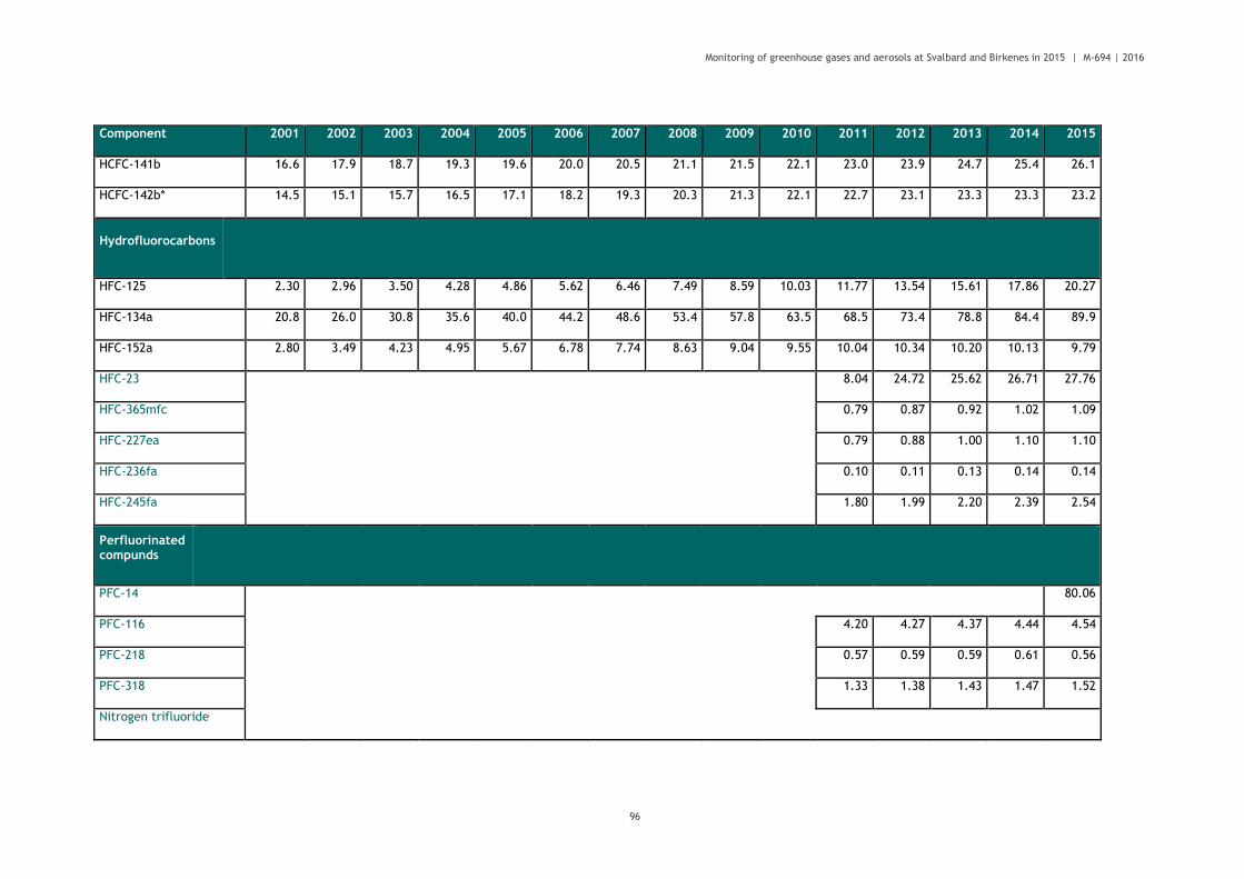
Monitoring of greenhouse gases and aerosols at Svalbard and Birkenes in 2015 | M-694 | 2016
96
Component 2001 2002 2003 2004 2005 2006 2007 2008 2009 2010 2011 2012 2013 2014 2015
HCFC-141b 16.6 17.9 18.7 19.3 19.6 20.0 20.5 21.1 21.5 22.1 23.0 23.9 24.7 25.4 26.1
HCFC-142b* 14.5 15.1 15.7 16.5 17.1 18.2 19.3 20.3 21.3 22.1 22.7 23.1 23.3 23.3 23.2
Hydrofluorocarbons
HFC-125 2.30 2.96 3.50 4.28 4.86 5.62 6.46 7.49 8.59 10.03 11.77 13.54 15.61 17.86 20.27
HFC-134a 20.8 26.0 30.8 35.6 40.0 44.2 48.6 53.4 57.8 63.5 68.5 73.4 78.8 84.4 89.9
HFC-152a 2.80 3.49 4.23 4.95 5.67 6.78 7.74 8.63 9.04 9.55 10.04 10.34 10.20 10.13 9.79
HFC-23 8.04 24.72 25.62 26.71 27.76
HFC-365mfc 0.79 0.87 0.92 1.02 1.09
HFC-227ea 0.79 0.88 1.00 1.10 1.10
HFC-236fa 0.10 0.11 0.13 0.14 0.14
HFC-245fa 1.80 1.99 2.20 2.39 2.54
Perfluorinated compunds
PFC-14 80.06
PFC-116 4.20 4.27 4.37 4.44 4.54
PFC-218 0.57 0.59 0.59 0.61 0.56
PFC-318 1.33 1.38 1.43 1.47 1.52
Nitrogen trifluoride

Monitoring of greenhouse gases and aerosols at Svalbard and Birkenes in 2015 | M-694 | 2016
97
Component 2001 2002 2003 2004 2005 2006 2007 2008 2009 2010 2011 2012 2013 2014 2015
Sulphurhexafluoride* 4.96 5.15 5.36 5.58 5.82 6.07 6.34 6.61 6.90 7.19 7.49 7.80 8.11 8.42 8.74
Halons
H-1211* 4.39 4.44 4.49 4.53 4.52 4.48 4.43 4.39 4.33 4.26 4.18 4.09 3.98 3.86 3.77
H-1301 2.99 3.06 3.12 3.17 3.21 3.24 3.26 3.28 3.29 3.31 3.32 3.34 3.36 3.38 3.42
Other halocarbons
Methylchloride 504.5 521.1 527.5 523.9 520.6 521.5 523.8 525.0 526.4 521.8 509.8 513.6 519.0 514.1 512.8
Methylbromide 8.93 9.08 8.94 8.92 8.61 8.60 8.35 7.77 7.37 7.28 7.20 7.02 6.95 6.85 6.89
Dichloromethane 30.9 31.0 32.0 32.0 31.7 33.1 35.1 37.2 38.2 41.8 42.2 45.2 53.9 54.5 54.1
Chloroform 10.9 10.6 10.7 10.5 10.5 10.5 10.6 10.4 10.8 11.4 11.9 12.0 12.7 13.4 13.7
Carbon tetrachloride 85.1 84.2 83.4 82.6 81.0
Methylchloroform 38.2 32.1 27.2 22.8 19.1 15.9 13.3 11.1 9.2 7.8 6.5 5.4 4.5 3.8 3.2
Trichloroethylene 0.67 0.58 0.40 0.45 0.39 0.38 0.29 0.32 0.51 0.52 0.54 0.51 0.55 0.48 0.33
Perchloroethylene 4.57 4.08 3.69 3.68 3.11 2.81 3.01 2.63 2.92 3.04 2.80 2.72 2.55 2.56 2.43
Volatile Organic Compounds (VOC)
Ethane 1466.8 1575.2 1565.7 1647.0 1651.4
Propane 170.9 520.6 548.9 574.9 566.0
Butane 182.8 187.2 202.4 190.0 184.4
Pentane 60.1 58.2 66.9 63.2 60.4

Monitoring of greenhouse gases and aerosols at Svalbard and Birkenes in 2015 | M-694 | 2016
98
Component 2001 2002 2003 2004 2005 2006 2007 2008 2009 2010 2011 2012 2013 2014 2015
Benzene 72.29 70.31 68.75 71.07 69.76
Toluene 28.54 24.59 25.83 27.87 25.75

Monitoring of greenhouse gases and aerosols at Svalbard and Birkenes in 2015 | M-694 | 2016
99
Table A 2: All calculated trends per year, standard error and regression coefficient for the fit. The trends are all in
pptv per year, except for CH4 N2O, and CO which are in ppbv. The negative trends are in blue, and the positive
trends are shown in red. Generally the period is from 2001-2015 but for the compounds marked in green, the
measurements started after September 2010. For these compounds, the trends are highly uncertain.
Component Formula Trend /yr Error R2
Carbon dioxide - Zeppelin
CO2
2.13 0.011 0.934
Carbon dioxide - Birkenes - - -
Methane - Zeppelin
CH4
5.23 0.056 0.835
Methane - Birkenes - - -
Carbon monoxide CO -1.29 0.063 0.794
Nitrous oxide N2O - - -
Chlorofluorocarbons
CFC-11* CCl3F -1.96 0.005 0.988
CFC-12* CF2Cl2 -2.1 0.015 0.925
CFC-113* CF2ClCFCl2 0.02 0.000 0.834
CFC-115* CF3CF2Cl 0.018 0.000 0.417
Hydrochlorofluorocarbons
HCFC-22 CHClF2 6.536 0.007 0.998
HCFC-141b C2H3FCl2 0.629 0.002 0.977
HCFC-142b* CH3CF2Cl 0.721 0.001 0.996
Hydrofluorocarbons
HFC-125 CHF2CF3 1.225 0.001 0.998
HFC-134a CH2FCF3 4.844 0.003 0.999
HFC-152a CH3CHF2 0.567 0.001 0.986
CHF3 1.017 0.002 0.997 CHF3
HFC-365mfc CH3CF2CH2CF3 0.072 0.000 0.981
HFC-227ea CF3CHFCF3 0.102 0.000 0.996
HFC-236fa CF3CH2CF3 0.012 0.000 0.952
HFC-245fa CHF2CH2CF3 0.196 0.001 0.992
Perfluorinated compunds
PFC-14 CF4 -1008.106 853.623 0.748
PFC-116 C2F6 0.082 0.000 0.982
PFC-218 C3F8 0.012 0.000 0.912
PFC-318 c-C4F8 -0.117 0.015 0.542
Sulphurhexafluoride* SF6 0.273 0.000 0.998

Monitoring of greenhouse gases and aerosols at Svalbard and Birkenes in 2015 | M-694 | 2016
100
Component Formula Trend /yr Error R2
Nitrogen trifluoride NF3 In 2016
Halons
H-1211* CBrClF2 -0.049 0.000 0.983
H-1301 CBrF3 0.026 0.000 0.760
Halogenated compounds
Methylchloride CH3Cl -0.279 0.071 0.858
Methylbromide CH3Br -0.184 0.002 0.866
Dichloromethane CH2Cl2 1.843 0.012 0.933
Chloroform CHCl3 0.207 0.003 0.805
Carbon tetrachloride CCl4 -0.912 0.019 0.645
Methylchloroform CH3CCl3 -2.342 0.002 0.999
Trichloroethylene CHClCCl2 -0.002 0.002 0.393
Perchloroethylene CCl2CCl2 -0.114 0.004 0.350
Non-methane hydrocarbons (NMHC) and Volatile Organic Compounds (VOC)
Ethane C2H6 38.7 4.835 0.908
Propane C3H8 7.72 4.252 0.847
Butane C4H10 0.97 2.080 0.761
Pentane C5H12 -0.38 0.763 0.693
Benzene C6H6 -3.7 0.400 0.879
Toluene C6H5CH3 -2.3 0.334 0.680

Monitoring of greenhouse gases and aerosols at Svalbard and Birkenes in 2015 | M-694 | 2016
101
Table A 3: Monthly means and standard deviation of aerosol optical depth (AOD) at 500 nm at Ny-Ålesund.’
Month/Year Mar Apr May Jun Jul Aug Sep
Aerosol optical depth (AOD)
2002 0.06±0.01 0.08±0.03 0.06±0.02 0.07±0.12 0.07±0.08 0.06±0.05
2003 0.15±0.12 0.11±0.05 0.15±0.06 0.10±0.03 0.04±0.01 0.05±0.02 0.06±0.03
2004 0.06±0.00 0.12±0.08 0.13±0.09 0.06±0.01 0.10±0.07 0.05±0.02 0.04±0.02
2005 0.08±0.03 0.12±0.07 0.10±0.03 0.05±0.02 0.05±0.02 0.04±0.03 0.03±0.01
2006 0.12±0.03 0.16±0.07 0.04±0.00 0.05±0.02 0.05±0.04 0.04±0.03
2007 0.10±0.05 0.10±0.12 0.07±0.03 0.05±0.01 0.05±0.02 0.04±0.03
2008 0.13±0.05 0.14±0.06 0.14±0.04 0.06±0.02 0.06±0.02 0.09±0.03 0.16±0.03
2009 0.11±0.03 0.08±0.02 0.11±0.04 0.10±0.02 0.09±0.01
2010 0.11±0.03 0.08±0.03 0.08±0.01 0.06±0.01 0.05±0.01 0.05±0.01
2011 0.08±0.02 0.08±0.01 0.05±0.01 0.06±0.02 0.05±0.01
2012 0.10±0.03 0.10±0.02 0.10±0.03 0.06±0.02 0.06±0.02 0.07±0.03 0.07±0.03
2013 0.11±0.04 0.09±0.04 0.06±0.02 0.05±0.01 0.06±0.02 0.05±0.01 0.04±0.02
2014 0.07±0.01 0.10±0.02 0.06±0.02 0.06±0.03 0.08±0.01 0.11±0.05
2015 0.05±0.02 0.10±0.03 0.07±0.02 0.05±0.01 0.15±0.20 0.05±0.02 0.05±0.01
Mean
(2002-2015) 0.10±0.04 0.10±0.04 0.10±0.04 0.06±0.02 0.07±0.04 0.06±0.03 0.06±0.03
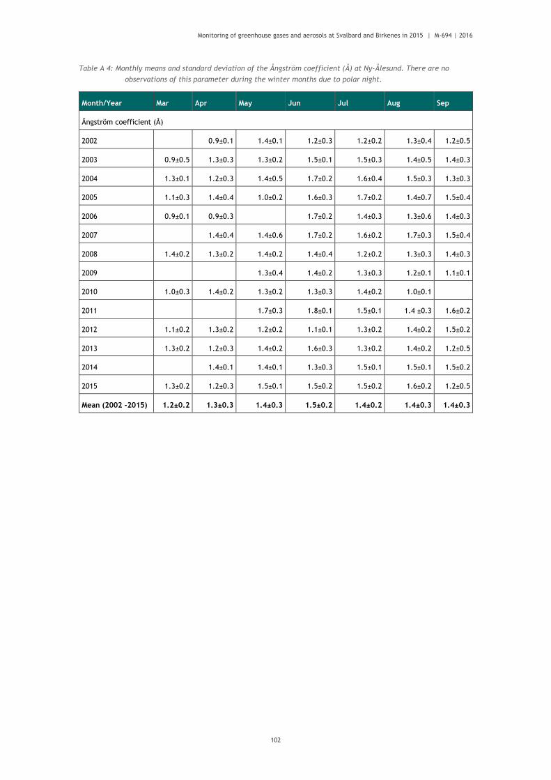
Monitoring of greenhouse gases and aerosols at Svalbard and Birkenes in 2015 | M-694 | 2016
102
Table A 4: Monthly means and standard deviation of the Ångström coefficient (Å) at Ny-Ålesund. There are no
observations of this parameter during the winter months due to polar night.
Month/Year Mar Apr May Jun Jul Aug Sep
Ångström coefficient (Å)
2002 0.9±0.1 1.4±0.1 1.2±0.3 1.2±0.2 1.3±0.4 1.2±0.5
2003 0.9±0.5 1.3±0.3 1.3±0.2 1.5±0.1 1.5±0.3 1.4±0.5 1.4±0.3
2004 1.3±0.1 1.2±0.3 1.4±0.5 1.7±0.2 1.6±0.4 1.5±0.3 1.3±0.3
2005 1.1±0.3 1.4±0.4 1.0±0.2 1.6±0.3 1.7±0.2 1.4±0.7 1.5±0.4
2006 0.9±0.1 0.9±0.3 1.7±0.2 1.4±0.3 1.3±0.6 1.4±0.3
2007 1.4±0.4 1.4±0.6 1.7±0.2 1.6±0.2 1.7±0.3 1.5±0.4
2008 1.4±0.2 1.3±0.2 1.4±0.2 1.4±0.4 1.2±0.2 1.3±0.3 1.4±0.3
2009 1.3±0.4 1.4±0.2 1.3±0.3 1.2±0.1 1.1±0.1
2010 1.0±0.3 1.4±0.2 1.3±0.2 1.3±0.3 1.4±0.2 1.0±0.1
2011 1.7±0.3 1.8±0.1 1.5±0.1 1.4 ±0.3 1.6±0.2
2012 1.1±0.2 1.3±0.2 1.2±0.2 1.1±0.1 1.3±0.2 1.4±0.2 1.5±0.2
2013 1.3±0.2 1.2±0.3 1.4±0.2 1.6±0.3 1.3±0.2 1.4±0.2 1.2±0.5
2014 1.4±0.1 1.4±0.1 1.3±0.3 1.5±0.1 1.5±0.1 1.5±0.2
2015 1.3±0.2 1.2±0.3 1.5±0.1 1.5±0.2 1.5±0.2 1.6±0.2 1.2±0.5
Mean (2002 -2015) 1.2±0.2 1.3±0.3 1.4±0.3 1.5±0.2 1.4±0.2 1.4±0.3 1.4±0.3

Monitoring of greenhouse gases and aerosols at Svalbard and Birkenes in 2015 | M-694 | 2016
103
Table A 5: Number of days with AOD observations at Ny-Ålesund made within the months.
Month/Year Mar Apr May Jun Jul Aug Sep
Number of days with cloud-free and quality assured observations
2002 4 15 11 6 9 14
2003 3 12 16 8 15 17 12
2004 2 8 13 9 5 12 12
2005 12 17 24 15 10 11
2006 6 12 5 12 4 13
2007 16 9 12 17 10 9
2008 15 12 14 20 16 13 2
2009 7 10 17 8 8
2010 7 18 7 10 12 3 1
2011 2 2 7 4 6
2012 6 18 12 15 16 11 4
2013 5 13 10 10 8 7 9
2014 13 9 9 9 14 4
2015 5 17 15 9 17 13 6
Total (2002-2015) 61 160 153 145 167 125 111
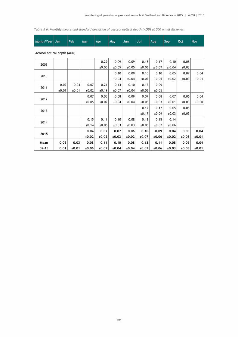
Monitoring of greenhouse gases and aerosols at Svalbard and Birkenes in 2015 | M-694 | 2016
104
Table A 6: Monthly means and standard deviation of aerosol optical depth (AOD) at 500 nm at Birkenes.
Month/Year Jan Feb Mar Apr May Jun Jul Aug Sep Oct Nov
Aerosol optical depth (AOD)
2009 0.29
±0.00
0.09
±0.05
0.09
±0.05
0.18
±0.06
0.17
± 0.07
0.10
± 0.04
0.08
±0.03
2010 0.10
±0.04
0.09
±0.04
0.10
±0.07
0.10
±0.05
0.05
±0.02
0.07
±0.03
0.04
±0.01
2011 0.02
±0.01
0.03
±0.01
0.07
±0.02
0.21
±0.19
0.13
±0.07
0.10
±0.04
0.13
±0.06
0.09
±0.05
2012 0.07
±0.05
0.05
±0.02
0.08
±0.04
0.09
±0.04
0.07
±0.03
0.08
±0.03
0.07
±0.01
0.06
±0.03
0.04
±0.00
2013 0.17
±0.17
0.12
±0.09
0.05
±0.03
0.05
±0.03
2014 0.15
±0.14
0.11
±0.06
0.10
±0.03
0.08
±0.03
0.13
±0.06
0.15
±0.07
0.14
±0.06
2015 0.04
±0.02
0.07
±0.02
0.07
±0.03
0.06
±0.02
0.10
±0.07
0.09
±0.06
0.04
±0.02
0.03
±0.03
0.04
±0.01
Mean
09-15
0.02
0.01
0.03
±0.01
0.08
±0.06
0.11
±0.07
0.10
±0.04
0.08
±0.04
0.13
±0.07
0.11
±0.06
0.08
±0.03
0.06
±0.03
0.04
±0.01

Monitoring of greenhouse gases and aerosols at Svalbard and Birkenes in 2015 | M-694 | 2016
105
Table A 7: Monthly means and standard deviation of the Ångström coefficient (Å) at Birkenes
Month/Year Jan Feb Mar Apr May Jun Jul Aug Sep Oct Nov
Ångström coefficient (Å)
2009 1.5
±0.0
1.2
±0.3
1.4
±0.3
1.4
±0.4
1.1
±0.2
1.0
±0.2
1.1
±0.2
2010 1.3
±0.3
1.4
±0.3
1.4
±0.2
1.4
±0.2
1.3
±0.3
1.3
±0.3
1.3
±0.23
2011 1.0
±0.2
1.0
±0.1
1.0
±0.3
1.2
±0.5
1.3
±0.3
1.5
±0.3
1.6
±0.3
1.6
± 0.1
2012 1.1
±0.4
1.6
±0.3
1.4
±0.4
1.7
±0.1
1.6
±0.3
1.5
±0.3
1.1
±0.3
1.4
±0.4
0.8
±0.3
2013 1.3
± 0.2
1.2
±0.3
0.8
±0.2
0.8
±0.3
2014 0.9
±0.5
1,0
±0.3
1.1
±0.3
1.0
±0.2
1.4
±0.3
1.1
±0.3
1.2
±0.2
2015 0.9
±0.2
1,1
±0.1
1.1
±0.2
1.3
±0.2
1.5
±0.2
1.4
±0.3
1.3
±0.2
1.2
±0.3
0.8
±0.3
Mean 09-
15
1.0
±0.1
1.0
±0.0
1.0
±0.3
1.2
±0.3
1.2
±0.2
1.4
±0.2
1.5
±0.3
1.3
±0.2
1.1
±0.2
1.2
±0.3
1.0
±0.3
Table A 8: Number of days with AOD observations at Birkenes made within the months.
Month/Year Jan Feb Mar Apr May Jun Jul Aug Sep Oct Nov
Number of days with cloud-free and quality assured observations (lev 2; lev 1.5 for 2013)
2009 1 22 25 11 13 15 12
2010 13 16 18 15 16 10 6
2011 7 2 20 23 18 20 15 13
2012 11 12 10 7 16 18 9 12 2
2013 26 18 13 7
2014 12 17 16 25 20 13 6
2015 6 1 14 21 21 16 9 11 3
Total 7 2 49 54 93 114 127 107 68 52 11

Monitoring of greenhouse gases and aerosols at Svalbard and Birkenes in 2015 | M-694 | 2016
106

Monitoring of greenhouse gases and aerosols at Svalbard and Birkenes in 2015 | M-694 | 2016
107
APPENDIX II
Description of instruments and
methodologies

Monitoring of greenhouse gases and aerosols at Svalbard and Birkenes in 2015 | M-694 | 2016
108

Monitoring of greenhouse gases and aerosols at Svalbard and Birkenes in 2015 | M-694 | 2016
109
In this appendix are the instrumental methods used for the measurements of the various
greenhouse gases presented. Additionally we explain the theoretical methods used in the
calculation of the trends.
Details about greenhouse gas measurements and recent improvement and extensions
Table A 9: Instrumental details for greenhouse gas measurements at Zeppelin and Birkenes.
Component Instrument and method
Time res.
Calibration procedures
Start - End Comment
Methane (Birkenes)
CH4 Picarro CRDS G1301 CO2/CH4/H2O
5 s Working std. calibrated against GAW stds at EMPA
19. May 2009 ->
Data coverage in 2015: 94%
Methane (Zeppelin)
CH4 GC-FID/ 1h NOAA reference standards
Aug 2001-Apr 2012
Methane (Zeppelin)
CH4 Picarro CRDS 5 sec NOAA reference standards
20.Apr. 2012 ->
Data coverage 2015: 92% (97%)
Nitrous oxide (Zeppelin)
N2O GC-ECD 30 min
Hourly, working std. calibrated vs. NOAA stds
Data coverage 2015 83% (86%)
Carbon monoxide (Zeppelin)
CO GC-HgO/UV 20 min
Every 20 min, working std. calibrated vs. GAW std.
Sep. 2001 - 2012
Discontinued after 2012
Carbon monoxide (Zeppelin)
CO Picarro CRDS 5 sec NOAA reference standards.
20.Apr 2012 ->
Data coverage 2015: 84% (89%)
Carbon dioxide (Zeppelin)
CO2 Picarro CRDS from 20.4.2012
1 h 5 sec
NOAA reference standards
1989 - 2012 20.Apr. 2012 ->
CO2 measurements in cooperation with ITM Stockholm University (SU). Data coverage 2015: 91% (95%)
Carbon dioxide (Birkenes)
CO2 Picarro CRDS G1301 CO2/CH4/H2O
5 s Working std. calibrated against GAW stds at EMPA
Measurements started 19 May 2009.
Data coverage in 2015: 94%
CFC-11 CFC-12 CFC-113 CFC-115 HFC-125 HFC-134a HFC-152a
HFC-365mfc
HCFC-22 HCFC-141b HCFC-142b H-1301 H-1211
CFCl3 CF2Cl2 CF2ClCFCl2 CF3CF2Cl CHF2CF3 CH2FCF3 CH3CHF2 CF3CH2CHF2CH3 CHF2Cl CH3CFCl2 CH3CF2Cl CF3Br CF2ClBr
ADS-GCMS 4 h
Every 4 hours, working std. calibrated vs. AGAGE std.
4.Jan 2001- 2010
This instrument was in operation from 04.01.2001 to 31.12.2010. The measurements of the CFCs have higher uncertainty and are not within the required precision of AGAGE. See next section for details.
Table cont.:

Monitoring of greenhouse gases and aerosols at Svalbard and Birkenes in 2015 | M-694 | 2016
110
Component Instrument and method
Time res.
Calibration procedures
Start - End Comment
Methyl Chloride Methyl Bromide Methylendichloride Chloroform Methylchloroform TriChloroethylene Perchloroethylene Sulphurhexafluoride
CH3Cl CH3Br CH2Cl2 CHCl3 CH3CCl3 CHClCCl2 CCl2CCl2 SF6
Tetrafluormethane
PFC-116
PFC-218
PFC-318
Sulphurhexafluoride Sulfuryl fluoride
HFC-23
HFC-32
HFC-125
HFC-134a
HFC-143a
HFC-152a
HFC-227ea
HFC-236fa
HFC-245fa
HFC-365mfc
HCFC-22
HCFC-124
HCFC-141b
HCFC-142b
CFC-11
CFC-12
CFC-113
CFC-114
CFC-115
H-1211
H-1301
H-2402
Methyl Chloride
CF4
C2F6 C3F8 c-C4F8
SF6
SO2F2
CHF3
CH2F2
CHF2CF3 CH2FCF3 CH3CF3 CH3CHF2
CF3CHFCF3
CF3CH2CF3
CF3CH2CHF2
CF3CH2CHF2CH3
CHF2Cl CHClFCF3 CH3CFCl2 CH3CF2Cl CFCl3 CF2Cl2 CF2ClCFCl2 CF2ClCF2Cl CF3CF2Cl CF3Br CF2ClBr CF2BrCF2Br
CH3Cl
CH3Br
CH3I
CH2Cl2
CHCl3
CH3CCl3
CH2Br2
CHBr3
TCE
PCE
C2H6
C3H8
C4H10
Medusa-GCMS No. 19
2 h
Every 2 hours, working std. calibrated vs. AGAGE std
01.09.2010->
Data coverage 2015: 60% due to break down of crucial parts.

Monitoring of greenhouse gases and aerosols at Svalbard and Birkenes in 2015 | M-694 | 2016
111
Component Instrument and method
Time res.
Calibration procedures
Start - End Comment
Methyl Bromide Methyl Iodide Methylendichloride Chloroform Methylchloroform Dibromomethane Bromoform TriChloroethylene Perchloroethylene
Ethane
Propane
n-Butane
n-Pentane
Benzene
Carbonyl Sulfide
C5H12
C6H6
COS
Ozone O3 5 min

Monitoring of greenhouse gases and aerosols at Svalbard and Birkenes in 2015 | M-694 | 2016
112
DATA QUALITY AND UNCERTAINTIES HALOCARBONS
In 2001 – 2010 measurements of a wide range of hydrochlorofluorocarbons,
hydrofluorocarbons (HCFC-141b, HCFC-142b, HFC-134a etc.), methyl halides (CH3Cl, CH3Br,
CH3I) and the halons (e.g. H-1211, H-1301) were measured with good scientific quality by
using ADS-GCMS. The system also measured other compounds like the chlorofluorocarbons,
but the quality and the precision of these measurements was not at the same level. Table A
10 shows a list over those species measured with the ADS-GCMS at Zeppelin Observatory. The
species that are in blue are of acceptable scientific quality and in accordance with
recommendations and criteria of the AGAGE network for measurements of halogenated
greenhouse gases in the atmosphere. Those listed in red have higher uncertainties and are not
within the required precision of AGAGE. There are various reasons for this increased
uncertainties; unsolved instrumental problems e.g. possible electron overload in detector (for
the CFC’s), influence from other species, detection limits (CH3I, CHClCCl2) and unsolved
calibration problems (CHBr3). Since 1.September 2010 the ADS-GCMS was replaced by a
Medusa-GCMS system. The uncertainties improved for almost all species (Table A 911 for
details), but there are periods where measurements of the CFC’s were still not satisfactory.
This is an unsolved problem within the AGAGE network.
Table A 10: ADS-GCMS measured species at Zeppelin from 4.January 2001 to 1. September 2010. Good scientific
quality data in Blue; Data with reduced quality data in Red. The data are available through http://ebas.nilu.no.
Please read and follow the stated data policy upon use.
Compound Typical
precision (%) Compound
Typical precision
(%)
SF6 1.5
H1301 1.5
HFC134a 0.4
H1211 0.4
HFC152a 0.6
CH3Cl 0.6
HFC125 0.8
CH3Br 0.8
HFC365mfc 1.7
CH3I 5.1
HCFC22 0.2
CH2Cl2 0.4
HCFC141b 0.5
CHCl3 0.3
HCFC142b 0.5
CHBr3 15
HCFC124 2.3
CCl4 0.5
CFC11 0.3
CH3CCl3 0.6
CFC12 0.3
CHClCCl2 1.2
CFC113 0.2
CCl2CCl2 0.7
CFC115 0.8

Monitoring of greenhouse gases and aerosols at Svalbard and Birkenes in 2015 | M-694 | 2016
113
Table below gives an overview over the species measured with the Medusa-GCMS systems at
the AGAGE stations and the typical precision with the different instruments. The Medusa-
GCMS instrument at the Zeppelin Observatory meet the same criteria as shown in the Table.
Table A 11: AGAGE measured species.
Compound Typical
precision (%) Compound
Typical precision
(%)
CF4 0.15 H1301 1.5
C2F6 0.9 H1211 0.5
C3F8 3 H2402 2
SF6 0.4 CH3Cl 0.2
SO2F2 1.6 CH3Br 0.5
HFC23 0.7 CH3I 2
HFC32 5 CH2Cl2 0.8
HFC134a 0.4 CHCl3 0.6
HFC152a 1.2 CHBr3 0.6
HFC125 1 CCl4 1
HFC143a 1.2 CH3CCl3 0.7
HFC365mfc 10 CHClCCl2 2.5
HCFC22 0.3 CCl2CCl2 0.5
HCFC141b 0.4 C2H2 0.5
HCFC142b 0.6 C2H4 2
HCFC124 2 C2H6 0.3
CFC11 0.15 C6H6 0.3
CFC12 0.05 C7H8 0.6
CFC13 2
CFC113 0.2
CFC114 0.3
CFC115 0.8

Monitoring of greenhouse gases and aerosols at Svalbard and Birkenes in 2015 | M-694 | 2016
114
METHANE
Methane is measured using a Picarro CRDS (Cavity Ring-Down Spectrometer) monitor which is
calibrated against NOAA reference standards. The instrument participates in yearly INGOS
cucumber ring tests. The continuous data are also compared to weekly flask samples sent to
NOAA CMDL, Boulder Colorado. All data will be available for download from the EBAS
database http://ebas.nilu.no.
N2O MEASUREMENTS
N2O is measured using a gas chromatograph with an electron capture detector. The
instrument is calibrated against NOAA reference standards. The instrument participates in
yearly INGOS cucumber ring tests and measurements are compared to weekly flask samples
sent to NOAA CMDL, Boulder Colorado. All data will be available for download from the EBAS
database http://ebas.nilu.no. The instrument is getting rather old, with increasing needs for
maintenance, but will soon be replaced by a new continuous measuring cavity ring-down
spectrometer with enhanced precision and much higher sample frequency.
CO2 MEASUREMENTS
At the Zeppelin station carbon dioxide (CO2) is monitored in cooperation with Stockholm
University (Institute of Applied Environmental Research, ITM). NILU is running the Picarro
Cavity Ring-Down Spectrometer used for continuous measurements, calibrated against SU-
ITM’s set of NOAA reference standards as a cooperation between the two institutes. The
instrument participates in yearly INGOS cucumber ring tests. The continuous data are also
compared to weekly flask samples sent to NOAA CMDL, Boulder Colorado. All data will be
available for download from the EBAS database http://ebas.nilu.no.
AIR INLET AT ZEPPELIN
In 2011 the air inlet for the GHG measurements at Zeppelin were improved to reduce possible
influence from the station and visitors at the station. The inlet was moved away from the
station and installed in a 15 m tower nearby for the following components:
N2O
CH4
CO2
CO
Halogenated compounds
NOAA flaks sampling program
Isotope flask sampling of CO2 and CH4
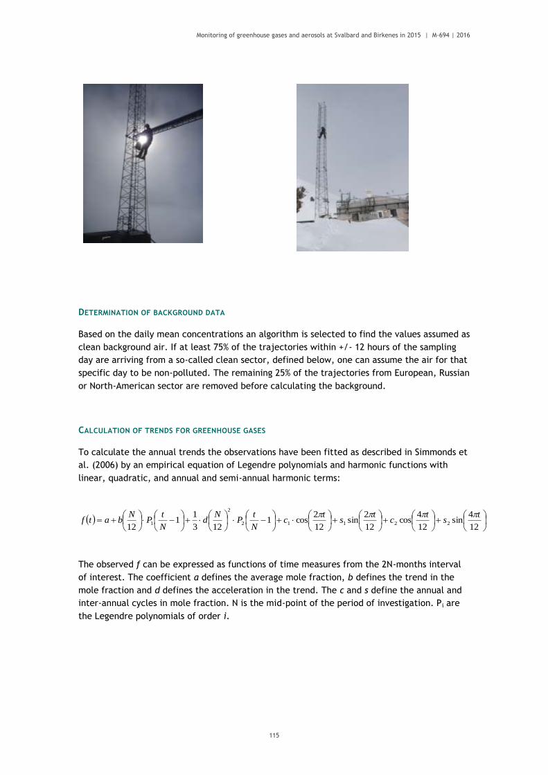
Monitoring of greenhouse gases and aerosols at Svalbard and Birkenes in 2015 | M-694 | 2016
115
DETERMINATION OF BACKGROUND DATA
Based on the daily mean concentrations an algorithm is selected to find the values assumed as
clean background air. If at least 75% of the trajectories within +/- 12 hours of the sampling
day are arriving from a so-called clean sector, defined below, one can assume the air for that
specific day to be non-polluted. The remaining 25% of the trajectories from European, Russian
or North-American sector are removed before calculating the background.
CALCULATION OF TRENDS FOR GREENHOUSE GASES
To calculate the annual trends the observations have been fitted as described in Simmonds et
al. (2006) by an empirical equation of Legendre polynomials and harmonic functions with
linear, quadratic, and annual and semi-annual harmonic terms:
12
4sin
12
4cos
12
2sin
12
2cos1
123
11
1222112
2
1
ts
tc
ts
tc
N
tP
Nd
N
tP
Nbatf
The observed f can be expressed as functions of time measures from the 2N-months interval
of interest. The coefficient a defines the average mole fraction, b defines the trend in the
mole fraction and d defines the acceleration in the trend. The c and s define the annual and
inter-annual cycles in mole fraction. N is the mid-point of the period of investigation. Pi are
the Legendre polynomials of order i.

Monitoring of greenhouse gases and aerosols at Svalbard and Birkenes in 2015 | M-694 | 2016
116
ON THE SURFACE IN SITU OBSERVATIONS OF AEROSOL MICROPHYSICAL AND OPTICAL PROPERTIES AT
BIRKENES
With respect to microphysical aerosol properties, the particle number size distribution (PNSD)
is observed at surface-level at Birkenes. The relevant and observed particle sizes cover a
range of 0.01 µm – 10 µm in particle diameter. The diameter range of 1.0 µm – 10 µm is
commonly referred to as coarse mode, the range Dp < 1.0 µm as fine mode. The fine mode is
separated further into Aitken-mode (0.01 µm < Dp < 0.1 µm) and accumulation mode (0.1 µm
< Dp < 1 µm). The distinction of these modes is justified by different predominant physical
processes as function of particle size. In the Aitken-mode, particles grow by condensation of
precursor gases from the gas-phase, and coagulate among themselves or with accumulation
mode particles. Accumulation mode particles grow by taking up Aitken-mode particles or by
mass uptake while being activated as cloud droplets, and they are removed by precipitation.
Coarse mode particles in turn are formed by break-up of biological or crustal material,
including pollen, bacteria, and fungus spores, and removed by gravitational settling and wet
removal. The PNSD of an aerosol is needed for quantifying any interaction or effect of the
aerosol since all of them depend strongly on particle size.
To measure the PNSD at Birkenes, 2 measurement principles are combined. A Differential
Mobilty Particle Spectrometer (DMPS) measures the particle number size distribution, now in
the range of 0.01 – 0.8 µm particle diameter after several improvements of the instrument. In
a DMPS, the particles in the sample air stream are put into a defined state of charge by
exposing them to an ionised atmosphere in thermal equilibrium. The DMPS uses a cylindrical
capacitor to select a narrow size fraction of the particle phase. The particle size in the
selected size fraction is determined by the voltage applied to the capacitor. The particle
number concentration in the selected size fraction is then counted by a Condensation Particle
Counter (CPC). A mathematical inversion that considers charge probability, diffusional losses
of particles in the system, transfer function of the capacitor, and counting efficiency of the
CPC is then used to calculate the particle number size distribution. The PNSD of particles with
diameters 0.25 µm < Dp < 30 µm is measured with an Optical Particle Spectrometer (OPS). In
the OPS, the particles in the sample stream are focussed through a laser beam. The
instrument registers number and amplitude of the pulses of light scattered by the particles.
The particle pulses are sorted into a histogram by their amplitude, where the pulse amplitude
yields the particle diameter and the pulse number the particle concentration, i.e. together
the PNSD. Both, the DMPS and the OPS, yield method specific measures of the particle
diameter, the electrical mobility and the optical particle diameter, respectively. When
related to the spherical equivalent geometric particle diameter commonly referred to, both
particle size measures depend on particle shape (causing a 5% systematic uncertainty in
particle diameter), the optical particle diameter in addition on particle refractive index
(causing a 20% systematic uncertainty in particle diameter). In this report, the PNSDs
provided by DMPS and OPS are joined into a common PNSD. To quality assure this process,
PNSDs are accepted only if DMPS and OPS PNSD agree within 25% in particle diameter in their
overlap size range. Together, both instruments provide a PNSD that spans over 3 orders of
magnitude in particle diameter, and over 6 orders of magnitude in particle concentration.
Another microphysical property measured at Birkenes is the Cloud Condensation Nuclei (CCN)
Concentration, i.e. the concentration of particles that could act as condensation nuclei for
liquid-phase cloud droplets, which is a property depending on the water vapour
supersaturation. The corresponding instrument, a Cloud Condensation Nucleus Counter
(CCNC), exposes the aerosol sample to an “artificial cloud” of defined supersaturation, and
Monitoring of greenhouse gases and aerosols at Svalbard and Birkenes in 2015 | M-694 | 2016
117
counts the cloud activated particles optically. Observations of the CCN concentration are
essential for quantifying the indirect aerosol climate effect. The CCNC at Birkenes has been in
operation since 2012, but is currently not included in the monitoring programme.
Optical aerosol parameters quantify the direct aerosol climate effect. The observation
programme at Birkenes includes the spectral particle scattering coefficient σsp(λ) and the
spectral particle absorption coefficient σap(λ). The scattering coefficient quantifies the
amount of light scattered by the aerosol particle population in a sample per distance a light
beam travels through the sample. The absorption coefficient is the corresponding property
quantifying the amount of light absorbed by the particle population in the sample. An
integrating nephelometer is used for measuring σsp(λ) at 450, 550, and 700 nm wavelength. In
this instrument, the optical sensors look down a blackened tube that is filled with aerosol
sample. The tube is illuminated by a light source with a perfect cosine intensity characteristic
perpendicularly to the viewing direction. It can be shown mathematically that this setup
integrates the scattered light seen by the optical sensors over all scattering angles. The
particle absorption coefficient σap(λ) is measured by 2 Particle Soot Absorption Photometers
(PSAPs). A PSAP infers σap(λ) by measuring the decrease in optical transmissivity of a filter
while the filter is loaded with the aerosol sample. The transmissivity time series is
subsequently translated into an absorption coefficient time series by using Lamber-Beer’s
law, the same law also used in optical spectroscopy. The PSAPs deployed at Birkenes are a
home-built 1 wavelength version that has received quality assurance by intercomparisons
within the EU network and infrastructure projects EUSAAR (European Supersites for
Atmospheric Aerosol Research) and ACTRIS (Aerosols, Clouds, and Trace gases Research
InfraStructure Network), and a 3-wavelength version. Both instruments are interpreted in
combination to benefit from both, quality assurance in a research network and spectral
capabilities. For comparison with the nephelometer, the PSAP data has been transferred to a
wavelength of 550 nm assuming an absorption Ångström coefficient åap of -1, adding 2%
systematic uncertainty to the data. The correction factor found for one Birkenes PSAP during
the recent intercomparison workshop has been included in the analysis.
All in situ observations of aerosol properties representing the ground-level are conducted for
the aerosol at dry-state (RH < 40%) for obtaining inter-comparability across the network.
DETAILS ABOUT AEROSOL OPTICAL DEPTH MEASUREMENTS
The amount of particles in the air during sunlit conditions is continuous monitored by means
of a Precision-Filter-Radiometer (PFR) sun photometer, located at the Sverdrup station in Ny-
Ålesund and a Cimel instrument at Birkenes. The observations in Ny-Ålesund are performed in
collaboration with PMOD/WRC (C. Wehrli), Davos, Switzerland. The main instrument
characteristics are given below.

Monitoring of greenhouse gases and aerosols at Svalbard and Birkenes in 2015 | M-694 | 2016
118
AERONET - Cimel C-318
Sun (9 channels) and sky radiances
Wavelength range: 340-1640 nm
15 min sampling
No temperature stabilization
AOD uncertainty: 0.01-0.02
PFR-GAW- Precision Filter Radiometer
Direct sun measurements (4 channels)
Wavelength range: 368 - 862 nm
1 min averages
Temperature stabilized
AOD uncertainty: 0.01
Figure 48: Photos and typical features of the standard instrument of the AERONET (left panel) and GAW PFR network
instruments (right panel)
The sun-photometer measurements in Ny-Ålesund are part of the global network of aerosol
optical depth (AOD) observations, which started in 1999 on behalf of the WMO GAW program. The
instrument is located on the roof of the Sverdrup station, Ny-Ålesund, close to the EMEP station
on the Zeppelin Mountain (78.9°N, 11.9°E, 474 m a.s.l.). The Precision Filter Radiometer (PFR)
has been in operation since May 2002. In Ny-Ålesund, the sun is below 5° of elevation from 10
October to 4 March, limiting the period with sufficient sunlight to the spring-early autumn
season. However, during the summer months it is then possible to measure day and night if the
weather conditions are satisfactory. The instrument measures direct solar radiation in four
narrow spectral bands centered at 862 nm, 501 nm, 411 nm, and 368 nm. Data quality control
includes instrumental control like detector temperature and solar pointing control as well as
objective cloud screening. Measurements are made at full minutes are averages of 10 samples for
each channel made over a total duration of 1.25 seconds. SCIAMACHY TOMSOMI and OMI ozone
columns and meteorological data from Ny-Ålesund are used for the retrieval of aerosol optical
depth (AOD).
Aerosol optical depth measurements started at the new Birkenes observatory in spring 2009,
utilizing an automatic sun and sky radiometer (CIMEL type CE-318), with spectral interference
filters centered at selected wavelengths: 340 nm, 380 nm, 440 nm, 500 nm, 675 nm, 870 nm,
1020 nm, and 1640 nm. The measurement frequency is approximately 15 minutes (this
depends on the air-mass and time of day). Calibration was performed regularly about once
per year in Spain (RIMA-AERONET sub-network). GOA manages the calibration for RIMA-
AERONET sun photometers. In the context of ACTRIS (Aerosols, Clouds, and Trace
gases Research Infra Structure Network, an EU (FP7) project) Transnational Access instrument

Monitoring of greenhouse gases and aerosols at Svalbard and Birkenes in 2015 | M-694 | 2016
119
calibration has been completed 14 May 2013 and October/November 2014 at the GOA-UVA
(Spain) installation of the AERONET-EUROPE Calibration Service Centre. Raw data are
processed and quality assured centrally by AERONET. Data reported for 2009 - 2014 are
quality assured AERONET level 2.0 data, which means they have been pre- and post-field
calibrated, automatically cloud cleared and have been manually inspected by AERONET.
OUTLOOK ON OBSERVATIONS OF AEROSOL OPTICAL DEPTH IN NY-ÅLESUND BEYOND 2015
Two observational initiatives and collaborations should be mentioned here:
1. Collaborative observations between NILU and the Alfred Wegener Institute (AWI,
Germany) using a sun-photometer on top of the Zeppelin Mountain, which is a unique
opportunity to separate the boundary layer contribution from the total column, and thereby
get new insides into the contribution of local versus long-range transport of aerosols. AWI
financed the instruments, NILU had ordered the a solar-tracker in 2012, but due to long
delivery times, only in spring 2013, measurements on a more routine bases started. The
scientific evaluation of the data is ongoing and will be published potentially in 2016.
2. A major obstacle to obtaining a complete year around AOD climatology in the Arctic
arises from the long polar night. To fill gaps in the aerosol climatology plans are ongoing to
deploy and test a lunar photometer to Ny-Ålesund in autumn 2014. This is a collaborative
initiative between PMOD/WRC, ISAC-CNR, NILU and others. Seed money for this activity was
received from the Svalbard Science Forum for the SSF Strategic grant project Lunar Arctic
project # 236774. The project aimed at coordinated remote sensing of Polar aerosol: LUNAR
photometry was to be used to close the gap in the annual cycle of the ARCTIC aerosol
climatology and to develop Svalbard as satellite validation site. The project started 1 March
2014. It was finalized at the end of June 2015, after a successful Lunar Photometry
workshop 24 - 26 June 2015 at Valladolid University, Valladolid, Spain.
Figure 49: Moon PFR on the Kipp & Zonen tracker during the day (left, parking position) and during night-time
measurements (right).
The PFR instrument modified by PMOD-WRC was installed on a tracker model Kipp & Zonen
provided usually hosting a sun photometer. Figure 49 shows the instrument on the tracker
during day-time and night-time. Six lunar cycles were monitored: the first during February
2014, while the other 5 during winter 2014-2015. We collected data on 66 measurement
periods, from Moon-rise to Moon-set or from minimum-to-minimum elevation as in Polar
Regions no set-rise events are possible. Among these, we obtained 17 distinct good
measurement periods, due to the frequent occurrence of clouds. For further details see e.g.
Mazzola at al., 2015.

Monitoring of greenhouse gases and aerosols at Svalbard and Birkenes in 2015 | M-694 | 2016
120

Monitoring of greenhouse gases and aerosols at Svalbard and Birkenes in 2015 | M-694 | 2016
121
APPENDIX III: Abbreviations

Monitoring of greenhouse gases and aerosols at Svalbard and Birkenes in 2015 | M-694 | 2016
122

Monitoring of greenhouse gases and aerosols at Svalbard and Birkenes in 2015 | M-694 | 2016
123
Abbreviation Full name
ACSM-ToF Aerosol Chemical Speciation Monitor
ACTRIS Aerosols, Clouds, and Trace gases Research InfraStructure Network
ADS-GCMS Adsorption-Desorption System – Gas Chromatograph Mass
Spectrometer
AeroCom Aerosol Comparisons between Observations and Models
AERONET Aerosol Robotic Network
AGAGE Advanced Global Atmospheric Gases Experiment
AIRS Atmospheric Infrared Sounder
AMAP Arctic Monitoring and Assessment
AOD Aerosol optical depth
AWI Alfred Wegener Institute
BC Black carbon
CAMP Comprehensive Atmospheric Monitoring Programme
CCN Cloud Condensation Nuclei
CCNC Cloud Condensation Nucleus Counter
CFC Chlorofluorocarbons
CICERO Center for International Climate and Environmental Research - Oslo
CIENS Oslo Centre for Interdisciplinary Environmental and Social Research
CLTRAP Convention on Long-range Transboundary Air Pollution
CO Carbon monoxide
CPC Condensation Particle Counter
DMPS Differential Mobility Particle
EMEP European Monitoring and Evaluation Programme
ENVRIplus Environmental Research Infrastructures Providing Shared Solutions
for Science and Society
EOS Earth Observing System
ERF Effective radiative forcing ERF
ERFaci ERF due to aerosol–cloud interaction
EU European Union
EUSAAR European Supersites for Atmospheric Aerosol Research
FLEXPART FLEXible PARTicle dispersion model
GAW Global Atmosphere Watch
Monitoring of greenhouse gases and aerosols at Svalbard and Birkenes in 2015 | M-694 | 2016
124
Abbreviation Full name
GB Ground based
GHG Greenhouse gas
GOA-UVA Atmospheric Optics Group of Valladolid University
GOSAT Greenhouse Gases Observing Satellite
GOSAT-IBUKI Greenhouse Gases Observing Satellite "IBUKI"
GWP Global Warming Potential
HCFC Hydrochlorofluorocarbons
HFC Hydrofluorocarbons
ICOS Integrated Carbon Observation System
InGOS Integrated non-CO2 Greenhouse gas Observing System
IPCC Intergovernmental Panel on Climate Change
ISAC-CNR Institute of Atmospheric Sciences and Climate (ISAC) of the Italian
National Research Council
ITM Stockholm University - Department of Applied Environmental
Science
JAXA Japan Aerospace Exploration Agency
LLGHG Well-mixed greenhouse gases
MOCA Methane Emissions from the Arctic OCean to the Atmosphere:
Present and Future Climate Effects
MOE Ministry of the Environment
NARE Norwegian Antarctic Research Expeditions
NASA National Aeronautics and Space Administration
NEOS-ACCM Norwegian Earth Observation Support for Atmospheric Composition
and Climate Monitoring
NIES National Institute for Environmental Studies
NOAA National Oceanic and Atmospheric Administration
NRS Norsk Romsenter
OC Organic Carbon
ODS Ozone-depleting substances
OH Hydroxyl radical
OPS Optical Particle Spectrometer
OSPAR Convention for the Protection of the marine Environment of the
North-East Atlantic
PFR Precision filter radiometer
PMOD/WRC Physikalisch-Meteorologisches Observatorium Davos/World Radiation
Center

Monitoring of greenhouse gases and aerosols at Svalbard and Birkenes in 2015 | M-694 | 2016
125
Abbreviation Full name
PNSD Particle number size distribution
ppb Parts per billion
ppm Parts per million
ppt Parts per trillion
PSAP Particle Soot Absorption Photometers
RF Radiative forcing
RI Research Infrastructure
RIMA Red Ibérica de Medida fotométrica de Aerosoles
SACC Strategic Aerosol Observation and Modelling Capacities for Northern
and Polar Climate and Pollution
SCIAMACHY SCanning Imaging Absorption spectroMeter for Atmospheric
CHartographY
SIS Strategisk instituttsatsing
SMPS Scanning Mobility Particle
TES Tropospheric Emission Spectrometer
TOA Top Of Atmosphere
TOMS OMI Total Ozone Mapping Spectrometer Ozone Monitoring instrument
UN United Nations
UNFCCC United Nations Framework Convention on Climate Change
VOC Volatile organic compounds
WDCA World Data Centre for Aerosol
WDCS World Data Centre of Aerosols
WMGHG Well-mixed greenhouse gases
WMO World Meteorological Organization

The Norwegian Environment Agency is working for
a clean and diverse environment. Our primary
tasks are to reduce greenhouse gas emissions,
manage Norwegian nature, and prevent pollution.
We are a government agency under the Ministry
of Climate and Environment and have 700
employees at our two offices in Trondheim and
Oslo and at the Norwegian Nature Inspectorate’s
more than sixty local offices.
We implement and give advice on the
development of climate and environmental
policy. We are professionally independent. This
means that we act independently in the individual
cases that we decide and when we communicate
knowledge and information or give advice.
Our principal functions include collating and
communicating environmental information,
exercising regulatory authority, supervising and
guiding regional and local government level,
giving professional and technical advice, and
participating in international environmental
activities.
Norwegian Environment Agency
Telephone: +47 73 58 05 00 | Fax: +47 73 58 05 01
E-mail: [email protected]
Web: www.environmentagency.no
Postal address: Postboks 5672 Sluppen, N-7485 Trondheim
Visiting address Trondheim: Brattørkaia 15, 7010 Trondheim
Visiting address Oslo: Grensesvingen 7, 0661 Oslo