Embed Size (px)
Citation preview

Lund University, Faculty of Engineering
Master thesisPHYM01
Fuel meter of the future
AuthorDavid Dahlgren
M.Sc. student in ElectricalEngineering, [email protected]
SupervisorsMikkel Brydegaard
Combustion Physics, [email protected]
Gustaf Gustafsson
Dover Fueling [email protected]
In collaboration with
Dover fueling solutions
June 11, 2019

Abstract
The purpose of this master thesis is to evaluate technologies that could mea-sure parameters of interest to Dover Fueling Solutions, a fuel pump company.A list of interesting measuring technologies has been compiled and compared.Spectrometry was chosen as extra interesting, as it had the potential to dif-ferentiate fuels by different octane ratings, but also measure concentrationsof different contents. A simplified spectrometer circuit setup was constructedand tested on different types of fuels. However, the results did not unambigu-ously show that different octane rated fuels could be differentiated. This wasprobably due to construction flaws. The project has shown the simplicity ofthe technology, but needs further testing and evaluation. The technology isdefinitely relevant to Dover Fueling Solutions and has potential to generatepositive value for the company and future costumers.
I

Acknowledgements
A special thanks to Gustaf Gustafsson for being a great mentor during theproject. Also thanks to Mikkel Brydegaard for providing his special skills andknowledge, it would not have been possible without him. Also a very specialthanks to Helena Sletten and our son Uno for making rainy days shine bright.
II

Contents
1 Introduction 1
1.1 Background . . . . . . . . . . . . . . . . . . . . . . . . . . . . . 1
1.2 Purpose and aim . . . . . . . . . . . . . . . . . . . . . . . . . . 2
1.3 Limitations . . . . . . . . . . . . . . . . . . . . . . . . . . . . . 2
1.4 Thesis disposition . . . . . . . . . . . . . . . . . . . . . . . . . . 3
2 Comparing technologies 4
2.1 Technologies . . . . . . . . . . . . . . . . . . . . . . . . . . . . . 5
2.1.1 Angular momentum meter for mass flow . . . . . . . . . 5
2.1.2 Capacitance measuring . . . . . . . . . . . . . . . . . . . 6
2.1.3 Coriolis meter . . . . . . . . . . . . . . . . . . . . . . . . 6
2.1.4 Drag Force Flow Sensors . . . . . . . . . . . . . . . . . . 7
2.1.5 Electrical conductivity . . . . . . . . . . . . . . . . . . . 8
2.1.6 Electromagnetic flow Sensors . . . . . . . . . . . . . . . 8
2.1.7 Laser-doppler-anemometer, LDA . . . . . . . . . . . . . 9
2.1.8 Microwave Absorbency . . . . . . . . . . . . . . . . . . . 9
2.1.9 NIR-field Spectrometry . . . . . . . . . . . . . . . . . . . 9
2.1.10 Nuclear Magnetic Resonance . . . . . . . . . . . . . . . . 11
2.1.11 Pressure Gradient Technique . . . . . . . . . . . . . . . . 11
2.1.12 Thermal Transport Sensors . . . . . . . . . . . . . . . . 12
2.1.13 Turbine-Based Flow Sensors . . . . . . . . . . . . . . . . 13
2.1.14 Ultrasound . . . . . . . . . . . . . . . . . . . . . . . . . 13
2.1.15 Vortex-Shedding flow meters . . . . . . . . . . . . . . . . 14
2.2 Technology compilation table . . . . . . . . . . . . . . . . . . . 15
2.3 Technology selection . . . . . . . . . . . . . . . . . . . . . . . . 16
3 Technology implementation 17
3.1 Circuit . . . . . . . . . . . . . . . . . . . . . . . . . . . . . . . . 17
3.1.1 Sender . . . . . . . . . . . . . . . . . . . . . . . . . . . . 18
3.1.2 Receiver . . . . . . . . . . . . . . . . . . . . . . . . . . . 19
3.2 Simulation . . . . . . . . . . . . . . . . . . . . . . . . . . . . . . 20
3.3 Construction . . . . . . . . . . . . . . . . . . . . . . . . . . . . 20
3.4 Testing . . . . . . . . . . . . . . . . . . . . . . . . . . . . . . . . 21
4 Result 25
III

5 Discussion 275.1 Future work . . . . . . . . . . . . . . . . . . . . . . . . . . . . . 28
6 Conclusion 29
References 29
Appendix
A Data sheetsA.0.1 Laser diode 1170 nm . . . . . . . . . . . . . . . . . . . .A.0.2 Laser diode 1170 nm . . . . . . . . . . . . . . . . . . . .A.0.3 Laser diode 1300 nm . . . . . . . . . . . . . . . . . . . .A.0.4 Laser diode 1300 nm . . . . . . . . . . . . . . . . . . . .A.0.5 FCI-InGaAs-500 photodiode nm . . . . . . . . . . . . . .
B Matlab code
IV

1
Introduction
1.1 Background
Dover Fueling Solution (DFS) is a fuel pump conglomerate with it’s base inAustin, Texas. Their products, which can be seen in Figure 1.1, can be found
Figure 1.1: Fuel pumps - prod-ucts of Dover Fueling Solutions.
all over the world. At it’s Malmo sub-sidiary, they research new technologies. Cur-rently, the company sells pumps with greatvolume flow measuring ability using me-chanical discretization of the flow (Posi-tive Displacement Flow), they can mea-sure volume flow for several months with-out deviation. The preciseness is impor-tant, due to the liquids worth: any longterm deviation could prove costly for gasstation owners. In fact, the mechani-cal technique used today to measure thevolume flow is difficult to develop anyfurther, and DFS is looking to measurethe flow using other technologies, and atthe same time look at other parametersthat could be of interest to their cus-tomers. This is the base of this master the-sis.
Dover Fueling Solutions has customers allover the world, and each market has their ownregulations and directives. Most markets havecertain regulations concerning explosive risks,spillage risks, temperature operating rangesetc. This places many demands on the fuel
1

pumps. The fuel itself can also come with many variations: it could be diesel,biofuel, ethanol and gasoline with varying octane rating. The fuel flow hasmany properties: density, water content, mass flow, volume flow, flow velocity,octane rating, air bubbles content and viscosity among others.
These properties can be of interest to customers. Relevant questions for thecustomers could be if the fuel liquid volume is as expected? Is the octanerating correct? The value of the liquid attracts people who want to tamperwith the pumps, both those who buy it and those who sell it. Adulterationof fuel is also something to be aware of, particularly in developing countries.Adulterated fuel can damage motors and results in an increase of emissions[1]. This calls for a desire to validate the fuel content.
1.2 Purpose and aim
The purpose of this Master Thesis is to investigate potential parameters ofinterest for Dover Fueling Solutions and their customers. Important factorswill be feasibility, cost and life expectancy of different measuring technologies.A literature study will be done, and the research will result in a matrix, con-sisting of measuring techniques on one axis, and features on another.
When the matrix has been completed, one or two techniques will be chosendepending on what potential worth they can give. Factors that will be takeninto account when deciding technique to implement are primarily if they canmeasure more properties than one, if they are expensive and feasibility. Thechosen technique will be studied closer and implemented if possible.
1.3 Limitations
When researching different measuring technologies, some physical quantities ofinterest mentioned by Dover Fueling Solutions was mass flow, water content,air bubbles, octane rating, density and liquid flow velocity. These quantitieswas mentioned that could have an potential interest to customers. Some ofthem indirectly, such as liquid flow velocity which can be used to find the vol-ume flow using properties of the pipe and the liquid.
The idea was that the measurements should happen in real time, measure-ments should be taken on flowing liquid. This further limited the techniques.
2

1.4 Thesis disposition
The following part of this thesis, Section 2, Comparing technologies, is a smallliterature study which contains information about different types of technolo-gies. The technologies are summed up in a table in Section 2.2. One of thetechnologies is selected and focused on. Section 3, Technology implementa-tion, explains how the technology is implemented. It contains informationabout schematics, simulation, construction and testing. The results can befound in Section 4 and they will be discussed in Section 5. Finally, conclusionswill be drawn in Section 6. References and appendix can be found at the endof the thesis.
3

2
Comparing technologies
In the search for different ways to measure the quantities mentioned in Sec-tion 1.3, primarily special topic books about sensors were used. Also someimportant sources were found using internet searches and studies of articles.Reading through special topic books about sensors is a good way to acquirean overview of many relevant techniques. Sensor technologies is a field in con-stant development, and therefore newer sources of sensor knowledge would bepreferred, but could not always be found. Sources 10-15 years old are common.There is also no guarantee that the collected information about sensors is com-prehensive enough to cover them all, and some measuring technologies wereleft out because they were not applicable to this project due to irrelevance orobvious difficulty to apply, such as titration. Titration can yield informationabout the content of a liquid, but would be to slow a process.
When measuring flow of a liquid, you either measure mass flow (kg/s) orvolume flow (m3/s). Mass gives a better picture of the liquid, since it isindependent of pressure and temperature. Volume on the other hand is largerif the temperature is high. The energy content of a liquid, which is what isinteresting when it comes to fuel, is proportional to the mass. Therefore, onemight believe that when trading with expensive liquids such as fuels, theywould be sold per kg, but are as a matter of fact sold by the volume. This ismostly due to historical reasons. The volume is however usually compensatedto a reference temperature of 15 °C [2]. Mass flow measurement could still beinteresting and has therefore been included.
Dover Fueling Solutions currently measures the volume flow of the liquid usingPositive Displacement Flow meters, its principle is described in Figure 2.1.They do this with great accuracy and durability. It is difficult to compete withthe accuracy of this measurement technique using other techniques, however,DFS wants to investigate other technologies to measure volume flow as a wayto stay competitive. Is there a way to make the measuring in a cheaper waythan with their current pumps?
4

Figure 2.1: The Positive Displacement Flow meter is used to measure the volumeflow of a liquid. The technique can be implemented in many ways, but the principleis that the liquid is discretized and counted. This technique has been refined byDover Fueling Solutions to measure with great accuracy. Image source: [3], usedwith permission.
2.1 Technologies
The technologies in this section is listed in alphabetical order, and has beensummed up Table 2.1.
2.1.1 Angular momentum meter for mass flow
This is a way of measuring mass flow. By forcing a tangential movement on aflowing liquid, for instance by letting the liquid pass through a rotating wheelas in Figure 2.2, an expression with the flow of mass can be acquired:
T = G (vti · ri − vtu · ru) (2.1)
where T is driving momentum, G is the flow of mass, vti is tangential velocityof the liquid at the entrance of the wheel, vtu is tangential velocity of the liquidat the exit of the wheel and ri and ru are the distance of the liquid to the centerof the pipe. In the case where vti is zero and the wheel is long enough for vtuto become ωru, Equation 2.1 deflates to
|T | = G · ω · r2u
To acquire G you need to measure T and ω, which can be difficult. Usuallythese types of mass flow meters are therefore implemented differently than asin Figure 2.2 [3].
5

Figure 2.2: By forcing a tangential movement on a flowing liquid, the mass flow canbe acquired. Image source: [3], used with permission.
2.1.2 Capacitance measuring
Capacitance can be used to measure water content in liquids, but can also beused to detect bubbles. The expression for capacitance in a capacitor is
C = εrε0A
d
where ε0 is the permittivity in vacuum, εr is the relative permittivity for thematerial between the capacitor plates, A is the plate area and d is the distancebetween the plates. The varying term in this case is εr. Imagine if the materialbetween the plates in a capacitor was a flow of pure gasoline, the capacitancewould be a certain value. If the flow instead changed to a gasoline dilutedwith water, the relative permittivity would change and therefore also the ca-pacitance [4]. However, if an air bubble (or other pollutant) passed in thecapacitor, the capacitance would also change [5]. Possibly both water contentand bubbles could be detected by measuring the capacitance, if it’s well un-derstood how much bubbles of different sizes affect the capacitance combinedwith different water contents.
2.1.3 Coriolis meter
A Coriolis meter (Figure 2.3) utilizes the Coriolis effect, and is the dominatingway to directly measure mass flow rate. The liquid runs through one or twotubes with certain shapes, typically U-shape, and the tubes are set in vibrationby some sort of driver. The flowing liquid forces the tubes to wobble (deflect)in a measurable way. The mass flow can then be acquired from the followingequation:
d = kfR (2.2)
where d is the relative net deflection of one tube compared to the other, kis a constant, f is the vibration frequency and R is the mass flow rate. Themain drawback of the Coriolis meter is that it is expensive compared to othertechnologies. It’s vibration also limits is life time [6].
6

Figure 2.3: The Coriolis meter. The flowing liquid is directed through the vibratingU-shaped tubes, which forces the tubes to wobble. The flow of mass can then beacquired from Equation 2.2. Image source: [7].
2.1.4 Drag Force Flow Sensors
If an object is inserted in a tube of flow, forces will act on it. If the object isconnected to the tube by a flexible beam, the acting force can be measuredusing strain gauges, and the velocity of liquid acquired using the followingformula:
ε =3CDρAV
2(L− x)
Ea2b(2.3)
where ε is the strain of the strain gauges, CD is a drag force coefficient, ρ is thedensity of the liquid, A is the area of the object projected on the flow, V is thevelocity of the liquid, L is the length of the beam, x is the where on the beamthe strain gauge is located, E is Young’s modulus of elasticity and a and bare some geometry target factors. The object could have different geometries,such as flat och spherical [8]. See Figure 2.4. A drawback is could be that youhave to know much about the system in advance to have all the variables inEquation 2.3.
7

Figure 2.4: A Drag Force Flow Sensor used to measure flow velocity. From “Hand-book of Modern Sensors” by Jacob Fraden. Used with permission.
2.1.5 Electrical conductivity
The electrical conductivity of gasoline with ethanol changes linearly with theconcentration of ethanol, at concentrations larger than about 25 %. The con-ductivity also changes with the concentrations of water [9]. In other word itshould be possible the measure the content of water or ethanol using anodeand cathode. Although it might not be worth the risk, putting an electricalcharge in highly flammable liquid could be risky and might not even be allowedby safety standards.
2.1.6 Electromagnetic flow Sensors
When a conductor moves through an magnetic field, it will induce a voltageaccording to Faraday’s law. The induced voltage can be used to acquire theflow rate, however, the liquid should be a good conductor, which is not thecase for gasoline (conductivity should be larger than 100 µS/m, but is a mere25 pS/m for gasoline [3, 10]). But if the fuel contains ethanol the conductivitygoes up, as mentioned in the previous section, and this method might then beapplicable. The magnetic flow sensor is generally expensive, but could be verysuitable for certain applications. For instance, it can tell in what directionthe flow is moving [11]. A sketch of principle can be seen in Figure 2.5. Thevelocity can be acquired using
v = e− e′ = 2aBv
where v is the velocity of liquid, a is the radius of the tube, e and e′ are inducedcurrents and B is the magnetic flow.
8

Figure 2.5: The principle of an electromagnetic flow sensor. The voltage will beinduced in the electrodes. B is the magnetic field and e and e’ are induced currents.From “Handbook of Modern Sensors” by Jacob Fraden. Used with permission.
2.1.7 Laser-doppler-anemometer, LDA
Laser-doppler-anemometers sends a beams of light into a flow, where some ofthe light will be reflected from particles in the flow. The particles could bebubbles or tracer particles. When the laser bounces on the moving particles,a doppler shift will be induced. This can be utilized to extract the velocityof the particles, and thus the flow rate. Generally, the LDA is expensive butreliable [3].
2.1.8 Microwave Absorbency
Microwave Absorbency can be used to measure water content. Water absorbsmicrowaves in the frequency of around 1-2 and 9-10 GHz. It can be detectwater from 1-70% with an accuracy of ± 0.5% [12].
2.1.9 NIR-field Spectrometry
Spectroscopy is a discipline which studies hows matter and light interacts. Itcan be used to determine content of substances by studying how they reflector absorb light with different wavelengths. Depending on how the substanceabsorbs or reflect energy in the light, conclusions can be drawn about thecontent of the substance. In terms of fuel, it can be used to determine octane
9

number and water content. It can also be used to predict viscosity and densityamong other things [13]. While spectrometry can refer to lights with anywavelength, fuels generally has their interesting characteristics in the Near-infrared (NIR) field. NIR refers to the region of 780 nm to 2500 nm in theelectromagnetic spectrum [14]. The spectrum for three different octane ratedfuels can be seen in Figure 2.6. The differences for the fuels can be used topredict their octane rating. NIR-spectrums can be complicated, but can beused to identify substances and quantities of i.e. water. Figure 2.7 showshow the spectrum varies for ethanol with different contents of water. Thismeasurement can be made very cost-efficient with LEDs as sources of light[15].
Figure 2.6: NIR-spectra for three different octane rated fuels. The R in the y-axisscale is reflectance. The curves for the three fuels are very alike, but differs slightly,and has been magnified between 1140 and 1155 nm. Image source: [16].
Octane rating is a property for a fuel, which tells how much pressure it canwithstand before igniting. A higher octane number generally means higherquality of the fuel. A low octane rated fuel can lead to problems with en-gine knocking [18]. The true octane number for a fuel is determined using astandardized motor, and cannot be done quickly. Therefore, spectrometry isinteresting as a way to predict octane rating faster and cheaper. It can beused in real time and with good precision. You can also look at specific wave-length of interest using laser diodes with the right wavelength, for instance inFigure 2.6, the magnified peak could be looked at. In order to avoid sampledependant variations such as turbidity, a comparison can be made between onemeasured intensity at a wavelength of interest and a normalized intensity, suchas another wavelength in the same sample wavelength or pure water [19, 15].
10

Figure 2.7: NIR-spectra for ethanol with differents contents of water. Blue line(uppermost) 90% ethanol, red line (middle) 95% ethanol and purple line (lowermost)100% ethanol. Image source: [17].
2.1.10 Nuclear Magnetic Resonance
Electromagnetic radiation can be applied to a liquid and the water moleculesset in resonance, if the frequency of the radiation is correct. The resonancein the molecules causes a loss in frequency power. This loss can be translatedto water content. However, other substances can also be set resonance thetherefore disturb the measurement [12].
2.1.11 Pressure Gradient Technique
Pressure gradient technique is a relatively common way to measure the volumeflow rate. The flow enters some kind of contraction and the change in pressureis measured. An expression for the flow can then be derived using Bernoulli’sprinciple, resulting in
q =A2√
1−(
A2
A1
)2 ·√
2 · (p1 − p2)ρ
where q is the volume flow, A1 and A2 are the tube flow area at the pressuresensors, p1 and p2 are pressures and ρ is the density of the flow. The contractioncan designed in several ways for different characteristics, one such can be seenin Figure 2.8 [3].
11

Figure 2.8: One design of the Pressure Gradient Technique. The change in pressurecan be measured and the volume flow acquired. Image source: Modern IndustriellMatteknik: GIVARE, used with permission.
2.1.12 Thermal Transport Sensors
One way to measure the mass flow is to see how fast heat disperses. Theprinciple is simple. At one point in the flow, put a heater, at another pointslightly further down the flow, put a thermometer, as in Figure 2.9. Dependingon what temperature is sensed, you can get an idea of how fast the flow is going.The faster the flow, the lower the temperature - the heat will dissipate faster.
Figure 2.9: Thermal transport sensor. The heat dissipates with the flow, and thedissipation can be measured with a thermometer, RS. This way, you can get a senseof the flow rate. R0 is also a thermometer, and is used to know the temperaturebefore heating. From “Handbook of Modern Sensors” by Jacob Fraden. Used withpermission.
12

2.1.13 Turbine-Based Flow Sensors
The turbine-based flow sensor is also simple in principle: allow the liquid flowto move propeller blades, and use hall sensors to measure how fast the bladesare rotating. The rotational speed of the turbine is proportional to the speed ofthe liquid. The faster the turbine is allowed to spin, the greater the resolution,but also shorter life time due to wear. If the turbine is designed to spin slowerit leads to a lower resolution but greater life expectancy. See Figure 2.10.
Figure 2.10: A turbine can be used to measure the velocity of a liquid. Image source:Modern Industriell Matteknik: GIVARE, used with permission.
2.1.14 Ultrasound
Ultrasound is a technique that can be used to obtain many different parametersof a liquid. It is also a relatively cheap and reliable technique. By sendingsound waves in the same direction as the flow, the speed of the liquid is addedto the speed of the sound. And by sending the sound waves in the oppositedirection of the flow, the speed of the liquid is subtracted from the speed ofthe sound. Therefore, by measuring the difference in time it takes the soundto traverse the both directions, you can extract the velocity of the flow. Atypical setup can be seen in Figure 2.11.
As with LDA, ultrasound can also be used to measure a doppler shift, andtherefore get a velocity of flowing particles, [8].
If the sound does not reach a microphone from the speaker, something must beobstructing the path. This could be utilized to detect air bubbles for instance[20].
Ultrasound can also be used to determine the density of the liquid. The speedof sound in liquid is
13

v =
√Ks
ρ
where Ks is a coefficient of stiffness in the medium and ρ is the density. Inother words, if Ks is known and v is measured, ρ can calculated, [21].
Figure 2.11: A typical setup for ultrasound flow meter. A and B are both transmit-ters and receivers of sound. The sound from A to B is faster than in the reverseddirection due to flow of the liquid. The difference in the speed of sound upstreamand downstream is proportional to the speed of the flow. From “Handbook of ModernSensors” by Jacob Fraden. Used with permission.
2.1.15 Vortex-Shedding flow meters
By obstructing the flow of a liquid with an object, vortex or eddies occurin the flow. The vertices are alternating, or shedding, on each side of theobstructing body, as depicted in Figure 2.12. The alternating vertices hasa frequency proportional to the velocity of the flow. So by measuring thealternating vertices, you can get an idea of the flow velocity. The measuringof the vertices can for example be made by ultrasound, thermal detection orpressure sensing, [3].
14

Figure 2.12: A vertex-shedding meter can be used to measure the flow velocity. Thevertices on each side of the obstructing body are alternating with a frequency propor-tional to the flow velocity. Image source: Modern Industriell Matteknik: GIVARE,used with permission.
2.2 Technology compilation table
Technology Mas
sflo
w
Wat
erco
nten
t
Bub
bles
Oct
anera
ting
Den
sity
Flow
velo
city
Angular Momentum Flow Meter X
Capacitance measuring X X
Coriolis meter X
Drag Force Flow Sensors X
Electrical Conductivity Meters X
Electromagnetic Flow Sensors X X
Laser-doppler-anemometer LDA X
Microwave Absorbency X
NIR-field Spectrometry X X
Nuclear Magnetic Resonance X
Pressure Gradient Technique X
Thermal Transport Senors X X X
Turbine-Based Flow Sensors X
Ultrasound X X X
Vortex-Shedding flow meters X
Table 2.1: A table showing the examined technologies that could be of interest toDover Fueling Solutions.
15
2.3 Technology selection
As can be seen in Table 2.1, some technologies can measure several quantities,and some quantities can only be measured by one technology. For instanceUltrasound could be used to detect bubbles, but also to measure density andflow velocity. Initially, NIR-field Spectrometry and Ultrasound was viewedas extra interesting. Spectrometry because it would be a great advantage forthe company if they could sell real time octane measuring to their customers,which would be something new to their market. At this point it was not clearif NIR-field spectrometry would turn out to be expensive and the feasibility ofit. Ultrasound on the other hand is a well established technique with betterknown pros and cons. It’s cheap and can measure several quantities, althoughnot necessarily with the same setup.
For the spectroscopy, one idea was to look at a single wavelength of interestinstead of an entire spectra, specifically a wavelength where the differencebetween different octane rated fuels are the greatest. This would simplify theimplementation. For gasoline, some potential wavelengths of interest could bearound 1150 nm, 1200 nm and 1400 nm, which can be seen as peaks in Figure2.6. Two wavelengths needs to be measured for it to work. The other is usedas a reference and should be somewhere where the amplitude does not varythat much, such as around 1300 nm in Figure 2.6, this is known as differentialabsorption [15, 19]. By dividing the acquired value at one wavelength bythe value at the other wavelength, variations in turbidity would be reduced.Looking at only a couple of wavelengths instead of an entire spectra wouldlargely simplify the technology, and make it cheaper and easier to construct.
Ultrasound is a well established technology, and several manufacturers andproducts exists on the market. There are several companies that suppliesindustrial process instrumentation and solutions.
The choice of technology to focus on ultimately fell on NIR-spectrometry. Themain reason being it’s a technology that could measure something difficult,octane rating, in a fast way. Dover Fueling Solutions expressed it has potentialto attract new customers.
16
3
Technology implementation
As discussed in section 2.1.9 and 2.3, a simplified spectrometer can be madethat would only look at two different wavelengths. To construct this simplifiedspectrometer three main parts are crucial: two light emitting sources withthe right wavelength and a photodiode sensitive to light in this region. Themedium of interest, the fuel, is in a container between the light source and thephotodiode.
If the difference in spectra for different octane rated fuels are as small as inFigure 2.6, then the light sources would have to emit light at in very shortspectra. Laser diodes can have this property, and has therefore been used inthis project.
3.1 Circuit
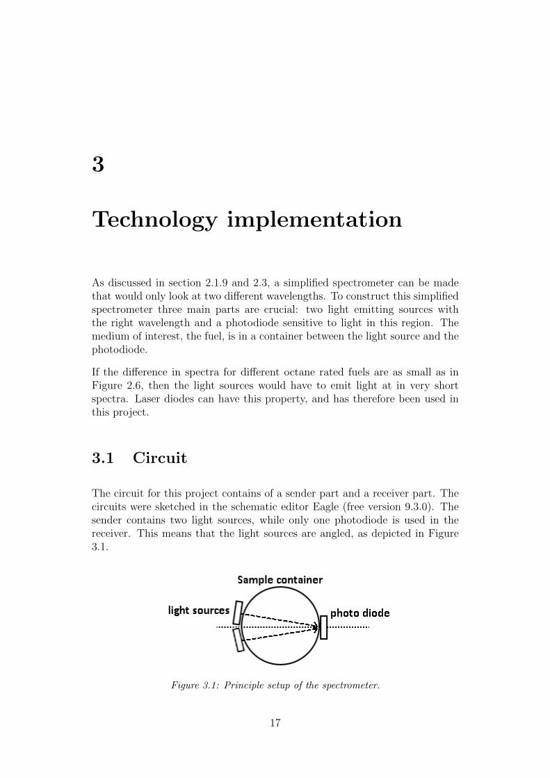
The circuit for this project contains of a sender part and a receiver part. Thecircuits were sketched in the schematic editor Eagle (free version 9.3.0). Thesender contains two light sources, while only one photodiode is used in thereceiver. This means that the light sources are angled, as depicted in Figure3.1.
Figure 3.1: Principle setup of the spectrometer.
17

3.1.1 Sender
Using a time-division multiplexing (TDM) scheme, the lasers alternated inemitting light with a selectable frequency. This is achieved using a counter(CD4017) that enables current to flow through the laser diodes by opening thetransistor, as can be seen in Figure 3.2. The counter puts all of its outputs inan on/off state one by one. First, the counter opens one of the transistor, acti-vating its connected laser, second the other transistor, third a ”black output”and finally it resets itself. The purpose of the ”black output” is to record thedark current from the background level. Some specifications of the used laserscan be found in Table 3.1. More can be found the Appendix A.0.1 and A.0.3.
Laser 1 Laser 2Peak wavelength [nm] 1172 1317Operating power [mW] 20 10Operation current [mA] 89 54Threshold current [mA] 48 27Model number FB-S1170-20SOT148 FB-S1300-10SOT148Supplier Fibercom Ltd Fibercom Ltd
Table 3.1: Some specifications of the lasers used.
The laser diodes are supplied with a constant current source, using the setupseen in the Figure with the LM317 voltage regulator. The flowing current willbe 1.25 volts divided by the size of the resistor, i.e. 15 Ω, resulting in 83.3 mA.
Figure 3.2: Schematics of the sender part. Two laser diodes alternating their trans-missions with the help of the counter and the transistors.
18
3.1.2 Receiver
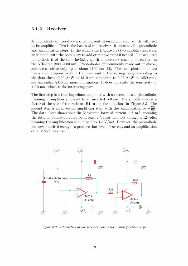
A photodiode will produce a small current when illuminated, which will needto be amplified. This is the basics of the receiver. It consists of a photodiodeand amplification steps. In the schematics (Figure 3.3) two amplification stepswere made, with the possibility to add or remove steps if needed. The acquiredphotodiode is of the type InGaAs, which is necessary since it is sensitive inthe NIR-area (800–2600 nm). Photodiodes are commonly made out of silicon,and are sensitive only up to about 1100 nm [22]. The used photodiode alsohas a lower responsitivity in the lower end of the sensing range according tothe data sheet (0.90 A/W at 1310 nm compared to 0.95 A/W at 1550 nm),see Appendix A.0.5 for more information. It does not state the sensitivity at1170 nm, which is the interesting part.
The first step is a transimpedance amplifier with a reverse biased photodiode,meaning it amplifies a current to an inverted voltage. The amplification is afactor of the size of the resistor, R1, using the notations in Figure 3.3. Thesecond step is an inverting amplifying step, with the amplification of −R22
R21.
The data sheet shows that the Maximum forward current is 8 mA, meaningthe total amplification could be at least 1 V/mA. The net voltage is 12 volts,meaning the amplification should be max 1.5 V/mA. However, the photodiodewas never excited enough to produce that level of current, and an amplificationof 50 V/mA was used.
Figure 3.3: Schematics of the receiver part, with 2 amplification steps.
19

3.2 Simulation
The simulation was made in the software LTspice XVII, see Figure 3.4. Thesimulation was made with two amplification steps and a total amplification of6 V/mA. The photodiode was simulated with a current signal generator. Thesimulation showed that the circuit was correctly designed, the voltage of theresistor R6 in Figure 3.4 was 6 times that of the current from I1.
Figure 3.4: Simulation in LTspice of the receiver circuit with two amplification steps.The photodiode was simulated with a current signal.
3.3 Construction
The construction of the circuits were made using stripboard prototype cards,which has parallel strips of copper coating. The physical layout was designedusing stripboard CAD program StripCAD 1.00. The designs can be seen inFigure 3.5 and 3.6. When it was finished, it was simply printed and put on thestripboard, then all the components and wires were soldered in place. Someminor design changes were made after the CAD-design.
The fuels were contained in glass test tubes with corks, and the holder forthe test tubes was a simple rubber ring with the right hole size. This rubberring held the laser diodes and the photodiode in place according to Figure 3.1.Therefore three holes with correct sizes were drilled in the rubber ring.
The constructed setup can be seen in Figure 3.7
20

Figure 3.5: StripCAD design of the sender.
Figure 3.6: StripCAD design of the sender.
3.4 Testing
In Sweden, fuels are usually 95 or 98 octane rated. Diesel is also common. Itwas decided that tests should be made on diesel, 95 and 98 rated fuel. Sampleswere collected from three different retailers: OKQ8, Preem and Ingo aroundMalmo, at a total of nine samples. The reason for multiple retailers is thatthere are many different fuel refineries, meaning the fuel can have differentturbidity and other optical properties. To make sure any findings of differenceis of significance, several different samples are important to use.
It was assumed that the spectra of acquired samples are the same as in Figure2.6. Other papers shows that the general structure of gasoline spectra is thesame. Figure 3.8 shows the spectra of several different octane rated fuels, it’ssimilar to Figure 2.6.
The samples were put in test tubes and the testing could commence. A functiongenerator with variable frequency was used as input to the counter. Thefrequency determines how long a counter output will be high before switchingto the next output, meaning the lasers will emit light with a period of the
21

Figure 3.7: The actual final setup. No sample in the rubber ring. The diameter ofthe holder hole is 21 mm. The outer diameter of the test tubes are 20 mm and theglass has a thickness of 1.25 mm.
Figure 3.8: The spectra of fuels with different octane ratings. Image source: [23]
22

inverse of this frequency.
The amplified signal was visualized with an Tektronix DPO 5104 oscilloscope.All nine samples was tested, and also an empty sample and a sample withtap water.A division between the 1170 nm amplified signal and the 1300 nmamplified signal will be calculated. The goal is to see if there is a difference ofsignificant between the three types of fuel. If that is the case, it would showthat technology could be of interest to Dover Fueling Solutions.
The reading of the values was done with the help of the oscilloscope. SeeFigure 3.9 as an example. In the Figure: a) The amplified signal when nolasers emits light (dark current), b) the amplified signal when the 1170 nmlaser emits light, c) the amplified signal when the 1300 nm laser emits lightand d) the counter switches. The oscilloscope was paused and a mean weretaken between two points. This was done with the help of the oscilloscopemean function, which calculates the mean between two lines; the green a andb in the figure. This was done on a), b) and c) in the Figure, and a mean ofthree different cycles was calculated. The lower levels, a) and b) were zoomedin with the help of the oscilloscope, for a better resolution. The image servesas an example and the values in it did not make it to the final results.
Figure 3.9: Oscilloscope screenshot of a measurement. a) The amplified signal whenno lasers emits light, b) the amplified signal when the 1170 nm laser emits light, c)the amplified signal when the 1300 nm laser emits light and d) the counter switches.This screenshot is an example and these values does not appear in the results.
When the values had been acquired, the dark current amplified signal wassubtracted and a division was calculated between the 1170 nm laser and the1300 nm laser amplified signal, according to Equation 3.1.
23
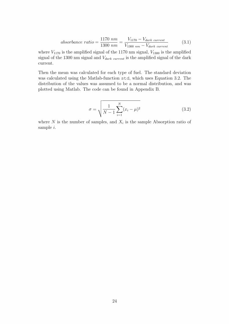
absorbance ratio =1170 nm
1300 nm=
V1170 − Vdark current
V1300 nm − Vdark current
(3.1)
where V1170 is the amplified signal of the 1170 nm signal, V1300 is the amplifiedsignal of the 1300 nm signal and Vdark current is the amplified signal of the darkcurrent.
Then the mean was calculated for each type of fuel. The standard deviationwas calculated using the Matlab-function std, which uses Equation 3.2. Thedistribution of the values was assumed to be a normal distribution, and wasplotted using Matlab. The code can be found in Appendix B.
σ =
√√√√ 1
N − 1
N∑i=1
(xi − µ)2 (3.2)
where N is the number of samples, and Xi is the sample Absorption ratio ofsample i.
24

4
Result
The collected values were compiled in the Table 4.1.
Type Origin No 1170 nm 1300 nm Absorption Typelaser laser [mv] laser [mv] ratio average
empty -0.26 36.4 234.4water -0.27 1.7 14.4
Preem -0.27 2.4 314.4 0.0085Diesel OKQ8 -0.26 2.4 298.4 0.0089
INGO -0.36 2.1 318.1 0.0078 0.0084Preem -0.35 3.7 258.1 0.0158
98 octane OKQ8 -0.36 3.3 259.8 0.0142INGO -0.33 4.6 196.5 0.0249 0.0183Preem -0.31 2.2 294.8 0.0084
95 octane OKQ8 -0.25 2.7 209.8 0.0139INGO -0.32 3.9 287.3 0.0146 0.0123
Table 4.1: The columns No laser 1170 nm laser and 1300 nm laser containsthe observed values of the amplified signal for the respective state. The values underAbsorption ratio has been calculated using Equation 3.1, that is, dividing theabsorption of the 1170 nm signal with the 1300 nm signal. Finally the right mostcolumns are average values of the type.
The expected (mean) values and standard variation has been calculated andcan be seen in Table 4.2.
Diesel 98 octane 95 octaneµ 0.0084 0.0183 0.0123σ 0.0006 0.0058 0.0034
Table 4.2: Expected value (µ) and standard deviation (σ) of the three fuel types.
The normal distribution plots using the values in Table 4.2 can be seen inFigure 4.1 and 4.2.
25

Figure 4.1: Using the values in Table 4.2, the normal distribution curves has beenplotted for 95 and 98 octane fuel.
Figure 4.2: Using the values in Table 4.2, the normal distribution curves has beenplotted for diesel. Note that the x-axis is much smaller than in Figure 4.1.
26

5
Discussion
The empty sample in Table 4.1 shows that the photodiode is much less sensitiveto the 1170 nm laser than the 1300 nm laser. According to the datasheet, A.0.5,the photodiode is slightly less sensitive in the lower region, but this does notexplain the vast differences between the 1170 nm laser and the 1300 nm laserthat also can be seen in the table. This is unfortunate, since that is the mostimportant part for this study. It does not mean however, that the values arenot interesting.
Looking at the Absorption ratio values shows that the values are somewhatconsistent. In both 95 and 98 octane two of the three values are close to eachother, while the third is a bit off. This explains why the standard deviationis relatively high and the why Normal Distribution curves overlap as can beseen in Figure 4.1. The diesel samples shows a more consistent result, andthe standard deviation is lower, which also shows in the Normal Distributioncurve in Figure 4.2. The peaks of the curves for 98 and 95 octane rated fuelsare located at different expected values, however since they overlap too much,it can’t be said that the difference between them is of a statistical significance.
It’s important to note, however, that the curves in Figure 4.1 and 4.2 arebased on only three samples. For a clearer result, more samples might berequired. The hope was that all curves would be similar in width as the onewith diesel, it would be much easier to say that the fuels can with a certaintybe differentiated using this technology.
Something important to comment on is the fact that the amplified 1300 nmsignal values of the fuels are in most cases larger than the empty sample.This indicates that more light gets through if there is a fuel in place, whichcould mean that the liquid and the curved glass focuses the light against thephotodiode. With only air in the test tube the differences in refractive indexescould diverge the beam.
The major reason for unclear results however, are probably due to flaws in theconstruction and testing setup. For one, the fuel container should not have
27

been circular, but rather flat. The laser light is bent and could be refractedby the round glass in an undesired way. Also, the laser don’t have lenses.According to the datasheet, the beam divergence of the lasers are 45° and 8°on each axis and 30° and 10° on each axis respectively (meaning they have anelliptical beam divergence). The lasers could be equipped with lenses to focusthe light for a better effect transfer. No care was taken about the orientationof the lasers. No shielding was done to the amplification circuit, which couldreduce the noise in the amplification.
During the measurements, it was noticed that the signal was very sensitiveto movements. During all readings and measurements the test tubes wereheld as straight and similar as possible, to reduce differences. Even very smalldifferences however, made relatively large changes in the amplified signal. Thisof course means there is a large variation from reading to reading. Using abetter built setup could improve the results greatly.
5.1 Future work
If Dover Fueling Solution chooses to continue with this technology, they shouldstart by designing the test setup in a better way. Use glass containers withflat surfaces. Build away sources of error and shield the construction fromdisturbances. Also, further amplifying steps could be added, such as ones thatzooms in on the signal levels and amplifies them. Noise reduction amplifierscould also be added. It could also be considered if different lasers should beused, are there better suited wavelengths to look at?
A spectrometer reading should be made on fuels of interest. It would be usefulif the spectra in Figure 2.6 could be verified. Do the local fuel differ muchor anything? In an end product, the fuel would probably be in a flowingstate. This might require the flow to be laminar. Also, since the lasers have aelliptical beam divergence, their orientation should be considered.
The lasers are sensitive to heat, and in a future iteration of this technology, itmight be important to add a heat control. Also, instead of using an oscilloscopeto manually read the results, it would probably be useful to have some sort ofdedicated data acquisition system, such as a Data Acquisition Card (DAQ) oran audio input.
28

6
Conclusion
The spectrometry technology has great potential for Dover Fueling Solutions.It has the possibility to verify the product - fuel - which is important for cus-tomers at all levels. Although the testings and measurements in this projectwas not as unambiguous as hoped, the result seem to indicate there is a dif-ference. It’s not unlikely a better prototype would show a clearer difference.The construction is relatively simple. It could relatively simply be integratedin future versions of the fuel pumps, and would be a good sales argument.
29

Bibliography
[1] Bhanu Prasad Vempatapu and Pankaj K. Kanaujia. Monitor-ing petroleum fuel adulteration: A review of analytical meth-ods. https://www.sciencedirect.com/science/article/abs/pii/S0165993616304174, 2017. Accessed 2019/02/05.
[2] Wikipedia. Fuel dispenser. https://en.wikipedia.org/wiki/Fuel_dispenser#The_metrology_of_gasoline, . Accessed2019/02/19.
[3] Lennart Grahm, Hans-Gunnar Jubring, and Alexander Lauber. ModernIndustriell Matteknik : GIVARE. Bokforlaget Teknikinformation, forthedition, 2007. Chapter 11.
[4] Shatha K. Jawad, Samah Z. Al-Rahamnah, Samir M. Said, Ayah A.Muwafi, and Ghada H. Al-Issawi. Capacitor meter to measure the percent-age of water in home diesel tank. https://www.researchgate.net/publication/287021991_Capacitor_meter_to_measure_the_percentage_of_water_in_home_diesel_tank, 2011.Accessed 2019/02/19.
[5] T. Vu Quoc, T. Pham Quoc, T. Chu Duc, T.T. Bui, K. Kikuchi, andM. Aoyagi. Capacitive sensor based on pcb technology for air bub-ble inside fluidic flow detection. https://ieeexplore.ieee.org/document/6984977, 2014. Accessed 2019/02/19.
[6] Alan S. Morris and Reza Langari. Measurement and InstrumentationTheory and Application. Academic Press, second edition, 2016. Section16.2.2.
[7] Wikipedia user Cleontuni. The vibration pattern with mass flow. doublesized version. https://en.wikipedia.org/wiki/Mass_flow_meter#/media/File:Coriolis_meter_vibrating_flow_512x512.gif. Accessed 2019/02/19.
[8] Jacob Fraden. Handbook of Modern Sensors, Physics, Designs and appli-cations. Springer-Verlag, third edition, 2003. Section 11.
[9] Michael Kass, Timothy J Theiss, Chris Janke, and Steven J Pawel.Analysis of underground storage tanks system materials to increased leak
30

potential associated with e15 fuel. https://www.researchgate.net/publication/255001707_Analysis_of_Underground_Storage_Tanks_System_Materials_to_Increased_Leak_Potential_Associated_with_E15_Fuel, 2012. Accessed2019/02/21.
[10] R Roberts, Roberts, and Roberts. Using properties to manage flammableliquid hazards. http://www.roberts-roberts.com/documents/Using%20Properties%20to%20Manage%20Flammable%20Liquid%20Hazards.pdf#page=3&zoom=100,0,600, 2011.Accessed 2019/02/22.
[11] William Hennessy. Sensor Technology Handbook. Chapter 10: Flow andLevel Sensors. Elsevier, first edition, 2005. Section Electromagnetic FlowSensors.
[12] Gert J.W. Visscher. Measurement, Instrumentation and Sensors Hand-book. Electromagnetic, Optical, Radiation, Chemical and Biomedical Mea-surement. CRC Press, second edition, 2014. Section 80.2.
[13] Guided wave. Why nir is better than gc. https://sales.guided-wave.com/nir-vs-gc/. Accessed 2019/03/04.
[14] Wikipedia. Near-infrared spectroscopy. https://en.wikipedia.org/wiki/Near-infrared_spectroscopy, . Accessed2019/03/04.
[15] Jesper Borggren. Combinatorial light path spectrometer for turbidliquids. https://lup.lub.lu.se/student-papers/search/publication/2260053, 2011. Accessed 2019/05/28.
[16] Durmus Ozdemir. Determination of octane number of gasoline usingnear infrared spectroscopy and genetic multivariate calibration meth-ods. https://doi.org/10.1081/LFT-200035547, 2005. Accessed2019/03/04.
[17] John Beauchaine and Jenni Briggs. Measurement of water in ethanol usingencoded photometric nir spectroscopy. http://eds.a.ebscohost.com.ludwig.lub.lu.se/eds/pdfviewer/pdfviewer?vid=3&sid=9854ce08-c3f8-40d0-966b-5408399e9f26%40sessionmgr4010, 2007. Accessed 2019/05/07.
[18] Wikipedia. Octane rating. https://en.wikipedia.org/wiki/Octane_rating, . Accessed 2019/03/04.
[19] Liang Mei and Mikkel Brydegaard. Continuous-wave differential ab-sorption lidar. https://onlinelibrary-wiley-com.ludwig.lub.lu.se/doi/epdf/10.1002/lpor.201400419, 2015. Ac-cessed 2019/05/28.
31
[20] Antonin Povolny, Hiroshige Kikura, and Tomonori Ihara. Ultrasoundpulse-echo coupled with a tracking technique for simultaneous mea-surement of multiple bubbles. https://www.ncbi.nlm.nih.gov/pubmed/29693582, 2018. Accessed 2019/04/02.
[21] Wikipedia. Speed of sound. https://en.wikipedia.org/wiki/Speed_of_sound#Equations, . Accessed 2019/04/02.
[22] Wikipedia. Photodiode. https://en.wikipedia.org/wiki/Photodiode#Materials, . Accessed 2019/05/09.
[23] www.azom.com. Determining the octane number using nir spec-troscopy. https://www.azom.com/article.aspx?ArticleID=17517. Accessed 2019/05/13.

Appendix A
Data sheets

-60 -40 -20 0 20 40 60
Pop
= 20mW
Intensity
,deg.
Diode laser in SOT-148 package
Model FB-S1170-20SOT148
Typical characteristics:
Sample 37-999
Parameter V a l u e U n i t
Threshold current, Ith 48 mA
Operating current, Iop 89 mA
Operating optical power, Рop 20 mW
Peak wavelength at Pop, λ 1172 nm
Beam divergence, (FWHM) 9 deg
Beam divergence, (FWHM) 30±3 deg
Feedback PD current ,IPD, 30 А
Feedback PD voltage <5 V
Operating regime CW
Operating temperature, Тop 25 oC
Package SOT-148
Beam divergence: Emitting spectra:
A.0.1 Laser diode 1170 nm

Fibercom LTD., Address: 2-nd Hutorskaya Str., 19, bld.2, Moscow, 127287, Russia Tel./Fax:+7 495 1070578, E-mail: [email protected], WEB: http://fbcom.ru
PRODUCT DATA SHEET
Laser Diode
Model FB-S1170-20SOT148
Specification Symbol Typical Unit
Laser Emitter
Peak Wavelength op 1170±20 nm
CW Optical Output Power Pop 20 mW
Operation Current Iop <110 mA
Operation Voltage Uld 1.3±0.3 V
Threshold Current Ith <60 mA
Beam Divergence (FWHM) θ 10±1 degree
Beam Divergence (FWHM) θ 30±5 degree
Spectrum Half-Width (FWHM) <5 nm
Emitting Area Wxd 4x1 µmxµm
Wavelength Temperature Coefficient ∆λ/∆T 3±0.2 Å/degree
Operation Power Temperature Coefficient ∆P/∆T 0.25±0.05 mW/degree
Operation Current Temperature Coefficient ∆I/∆T 0.3±0.05 mA/degree
Mode Structure SM TE00 -
Operation Temperature Top 25 degree
Operation Temperature Range -40… +50 degree
Storage Temperature Range -40… +80 degree
Operation Mode CW Pulse
Continuous Wave
Pulse, τ>5 ns
-
Photo Diode Monitor
Monitor Current 1-1000 µA
PD Reverse Voltage <5 V
Note: To guarantee reliable operation of laser diode SOT-148 package must be mounted onto copper
carrier with TEC (Peltier element) keeping constant temperature.
A.0.2 Laser diode 1170 nm

-80 -60 -40 -20 0 20 40 60 80
,deg.
Inte
nsit
y, a.u
.
||
_|_
Diode laser in SOT-148 package Model FB-S1300-10SOT148
Typical characteristics:
Sample 347-69
Parameter V a l u e U n i t
Threshold current, Ith 27 mA
Operating current, Iop 54 mA
Operating optical power, Рop 10 mW
Peak wavelength at Pop, λ 1317 nm
Beam divergence, (FWHM) 6 deg
Beam divergence, (FWHM) 43 deg
Feedback PD current ,IPD, 82 А
Feedback PD voltage <5 V
Operating regime CW
Operating temperature, Тop 25 oC
Package SOT-148
Beam divergence: Emitting spectra:
A.0.3 Laser diode 1300 nm

Fibercom LTD., Address: 2-nd Hutorskaya Str., 19, bld.2, Moscow, 127287, Russia Tel./Fax:+7 495 1070578, E-mail: [email protected], WEB: http://fbcom.ru
PRODUCT DATA SHEET
Laser Diode
Model FB-S1300-10SOT148
Specification Symbol Typical Unit
Laser Emitter
Peak Wavelength op 1300±30 nm
CW Optical Output Power Pop 10 mW
Operation Current Iop <80 mA
Operation Voltage Uld 1.1±0.2 V
Threshold Current Ith <40 mA
Beam Divergence (FWHM) θ 8±2 degree
Beam Divergence (FWHM) θ 45±5 degree
Spectrum Half-Width (FWHM) <2.5 nm
Emitting Area Wxd 5x1 µmxµm
Wavelength Temperature Coefficient ∆λ/∆T 4±0.5 Å/degree
Operation Power Temperature Coefficient ∆P/∆T 0.15±0.05 mW/degree
Operation Current Temperature Coefficient ∆I/∆T 0.4±0.05 mA/degree
Mode Structure SM TE00 -
Operation Temperature Top 25 degree
Operation Temperature Range -40… +50 degree
Storage Temperature Range -40… +80 degree
Operation Mode CW Pulse
Continuous Wave
Pulse, τ>5 ns
-
Photo Diode Monitor
Monitor Current 1-1000 µA
PD Reverse Voltage <5 V
Note: To guarantee reliable operation of laser diode SOT-148 package must be mounted onto copper
carrier with TEC (Peltier element) keeping constant temperature.
A.0.4 Laser diode 1300 nm

82
nAPPLICATIONS• High Speed Optical Communications• Single/Multi-Mode Fiber Optic Receiver• Gigabit Ethernet/Fibre Channel• SONET/SDH, ATM• Optical Taps
155Mbps/622Mbps/1.25Gbps/2.5GbpsHigh Speed InGaAs Photodiodes
FCI-InGaAs-XXX series with active area sizes of 55µm, 70µm, 120µm,
300µm, 400µm and 500µm, exhibit the characteristics need for Datacom
and Telecom applications. Low capacitance, low dark current and high
responsivity from 1100nm to 1620nm make these devices ideal for high-bit
rate receivers used in LAN, MAN, WAN, and other high speed communication
systems. The photodiodes are packaged in 3 lead isolated TO-46 cans or in
1 pin pill packages with AR coated flat windows or micro lenses to enhance
coupling efficiency. FCI-InGaAs-XXX series is also offered with FC, SC, ST
and SMA receptacles.
nFEATURES• High Speed• High Responsivity• Low Noise• Spectral Range 900nm to 1700nm
Electro-Optical Characteristics TA=23°C
PARAMETERS SYMBOL CONDITIONSFCI-InGaAs-55 FCI-InGaAs-70 FCI-InGaAs-120 FCI-InGaAs-300 FCI-InGaAs-400 FCI-InGaAs-500
UNITSMIN TYP MAX MIN TYP MAX MIN TYP MAX MIN TYP MAX MIN TYP MAX MIN TYP MAX
Active Area Diameter AAφ --- --- 55 --- --- 70 --- --- 120 --- --- 300 --- --- 400 --- --- 500 --- µm
Responsivity(Flat Window Package) Rλ
λ=1310nm 0.80 0.90 --- 0.80 0.90 --- 0.80 0.90 --- 0.80 0.90 --- 0.80 0.90 --- 0.80 0.90 ---A/W
λ=1550nm 0.90 0.95 --- 0.90 0.95 --- 0.90 0.95 --- 0.90 0.95 --- 0.90 0.95 --- 0.90 0.95 ---
Capacitance Cj VR = 5.0V --- 1.0 --- --- 1.5 --- --- 2.0 --- --- 10.0 --- --- 14.0 --- --- 20.0 --- pF
Dark Current Id VR = 5.0V --- 0.02 2 --- 0.03 2 --- 0.05 2 --- 0.30 5 --- 0.40 5 --- 0.50 20 nA
Rise Time/Fall Time tr/tf
VR = 5.0V, RL=50Ω
10% to 90%--- --- 0.20 --- --- 0.20 --- --- 0.30 --- --- 1.5 --- --- 3.0 --- --- 10.0 ns
Max. Revervse Voltage --- --- --- --- 20 --- --- 20 --- --- 20 --- --- 15 --- --- 15 --- --- 15 V
Max. Reverse Current --- --- --- --- 0.5 --- --- 1 --- --- 2 --- --- 2 --- --- 2 --- --- 2 mA
Max. Forward Current --- --- --- --- 5 --- --- 5 --- --- 5 --- --- 8 --- --- 8 --- --- 8 mA
NEP --- --- --- 2.66E-15 --- --- 3.44E-
15 --- --- 4.50E-15 --- --- 6.28E-
15 --- --- 7.69E-15 --- --- 8.42E-
15 --- W/√Hz
Absolute Maximum Ratings
PARAMETERS SYMBOL MIN MAX UNITS
Storage Temperature Tstg -55 +125 °C
Operating Temperature Top -40 +75 °C
Soldering Temperature Tsld --- +260 °C
A.0.5 FCI-InGaAs-500 photodiode nm

Appendix B
Matlab code
close allclear all
res diesel = [0.008469009, 0.008894502, 0.007758978];res 98 octane = [0.015779945, 0.014197599, 0.024874141];res 95 octane = [0.008359595, 0.013901452, 0.014582222];
std dies = std(res diesel);mean dies = mean(res diesel);
std 98 = std(res 98 octane);mean 98 = mean(res 98 octane);
std 95 = std(res 95 octane);mean 95 = mean(res 95 octane);
x = [-3:.001:3];y diesel = normpdf(x,mean dies , std dies);
figure(1)plot(x,y diesel)legend(’Diesel’)xlabel(’Absorption division’)
y 98octane = normpdf(x, mean 98 , std 98);y 95octane = normpdf(x, mean 95 , std 95);
figure(2)plot(x,y 98octane,’--’)hold onplot(x,y 95octane)

legend(’98 octane’, ’95 octane’)xlabel(’Absorption division’)