Embed Size (px)
Citation preview
LLSSFF RReesseeaarrcchh WWoorrkkiinngg PPaappeerr SSeerriieess
NN°°.. 1188--0022
The opinions and results mentioned in this paper do not reflect the position of the Institution.
The LSF Research Working Paper Series is available online: http://wwwen.uni.lu/recherche/fdef/luxembourg_school_of_ finance_research_in_finance/working_papers For editorial correspondence, please contact: [email protected]
University of Luxembourg Faculty of Law, Economics and
Finance Luxembourg School of Finance
6 rue Coudenhove Kalergi L-1359 Luxembourg
Date: January 2018
Title: A test of the Modigliani-Miller invariance theorem and arbitrage in experimental asset markets
Author(s)*: G. Charness & T. Neugebauer
Abstract : Modigliani and Miller (1958) show that a repackaging of asset return streams to
equity and debt has no impact on the total market value of the firm if pricing is arbitrage-
free. We test the empirical validity of this invariance theorem in experimental asset
markets with simultaneous trading in two shares of perfectly-correlated returns. Our data
support value invariance for assets of identical risks when returns are perfectly correlated.
However, exploiting price discrepancies has risk when returns have the same expected
value but are uncorrelated, and we find that the law of one price is violated in this case.
Discrepancies shrink in consecutive markets, but seem to persist even with experienced
traders. In markets where overall trader acuity is high, assets trade closer to parity.
JEL classification: C92, G12
Keywords: Modigliani-Miller theorem, asset market, twin shares, experiment, limits to arbitrage, perfect correlation, experience, cognitive reflection test, risk aversion
*Corresponding Author’s Address:
Tel: +352 46 66 44 62 85 Fax : +352 46 66 44 6835 E-mail address: [email protected]

A test of the Modigliani-Miller invariance theorem and arbitrage in experimental asset markets
Gary Charness & Tibor Neugebauer∗
Abstract: Modigliani and Miller (1958) show that a repackaging of asset return streams to equity
and debt has no impact on the total market value of the firm if pricing is arbitrage-free. We test
the empirical validity of this invariance theorem in experimental asset markets with simultaneous
trading in two shares of perfectly-correlated returns. Our data support value invariance for assets
of identical risks when returns are perfectly correlated. However, exploiting price discrepancies
has risk when returns have the same expected value but are uncorrelated, and we find that the
law of one price is violated in this case. Discrepancies shrink in consecutive markets, but seem
to persist even with experienced traders. In markets where overall trader acuity is high, assets
trade closer to parity.
Keywords: Modigliani-Miller theorem, asset market, twin shares, experiment, limits to arbitrage,
perfect correlation, experience, cognitive reflection test, risk aversion
JEL Codes: C92, G12
∗ Tibor Neugebauer is at the University of Luxembourg. Gary Charness is at University of California, Santa Barbara. The authors have no conflicts of interest to disclose. The authors obtained IRB approval for data collection. We gratefully acknowledge the helpful comments of Bruno Biais (the Editor), the anonymous Associate Editor, two anonymous reviewers, Peter Bossaerts, Martin Duwfenberg, Darren Duxbury, Catherine Eckel, Ernan Haruvy, Chad Kendall, Roman Kräussl, Ulf von Lilienfeld-Toal, Raj Mehra, Luba Petersen, Jianying Qiu, Kalle Rinne, Jean-Charles Rochet, Jason Shachat, Julian Williams for helpful comments. We also thank seminar participants at Durham Business School, University of Luxembourg, Radboud University of Nijmegen, and at the conferences Experimental Finance in Nijmegen, the Netherlands, Experimental Finance in Tucson, Arizona, the International Meeting on Experimental and Behavioral Sciences in Toulouse, France, Conference on Behavioural Aspects of Macroeconomics & Finance at House of Finance, Frankfurt, Germany, Barcelona GSE Summer Forum, Spain, and CESifo in Munich, Germany. The scientific research presented in this publication received financial support from the National Research Fund of Luxembourg (INTER/MOBILITY/12/5685107), and University of Luxembourg provided funding of the experiments through an internal research project (F2R-LSF-PUL-10IDIA).

1
Forthcoming in The Journal of Finance

2
In their seminal paper, Modigliani and Miller (1958, 1963) showed mathematically that the
market value of the firm is invariant to the firm’s leverage; different packaging of contractual
claims on the firm’s asset returns does not impact the total market value of the firm’s debt and
equity. The Modigliani and Miller – henceforth MM – value-invariance theorem suggests that
the law of one price prevails for assets of the same “risk class”. The core of the theorem is an
arbitrage proof: If two assets, one leveraged and one unleveraged, represent claims on the same
cash flow, any arising market discrepancies are arbitraged away. But due to its assumption of
perfect capital markets and the no-limits-to-arbitrage condition (requiring perfect positive
correlation of asset returns, no fees on the usage of leverage, etc.), the MM theorem has not been
tested in a satisfactory manner on real-world market data. Thus, its empirical significance has
been unclear.1
Nevertheless, such a test is feasible in the laboratory, and providing an empirical test of
the MM theorem is a primary purpose of this laboratory study. Since perfect return-correlation is
rare in naturally-occurring equities, we also check how limits to arbitrage affect the empirical
validity of the MM theorem with regards to cross-asset pricing. In particular, we address the
question of whether a perfect positive correlation between asset returns is necessary for the
empirical validity of value invariance or if the same expected (rather than identical) future return
is sufficient, as suggested for our setting by the capital asset pricing model. Our data indeed
suggest that perfect correlation is necessary for the law of one price to prevail.
1 The perfect-capital-markets assumption requires, among other things, that no taxes and transaction fees are levied, and that the same interest rate applies for everyone. Lamont and Thaler (2003) present several real-world examples where the law of one price is violated. They argue that these violations result from limits to arbitrage. There was an early objection concerning the applicability of value invariance in relation to the variation of payout policy. Modigliani and Miller (1959) replied to this objection by stating that the dividend policy is irrelevant for the value of the company. However, it is now widely-accepted that dividends impact empirical valuations (for a recent discussion of the dividend puzzle, see DeAngelo and DeAngelo 2006). The dividend-irrelevance theorem was thus empirically rejected and is considered as being of theoretical interest only. Still, the value-invariance theorem and its proof remain widely-accepted in the profession even without an empirical test.

3
Our main design adapts the experimental asset-markets research of Smith, Suchanek and
Williams (1988), featuring multi-period cash flows, zero interest rates, and a repetition of
markets with experienced subjects.2 However, in contrast to the standard, single-asset market
approach of Smith et al. and in line with MM, we have simultaneous trading taking place in two
shares of the same “equivalence class”. These twin shares, which we call the L-shares and the
U-shares, are claims on the same underlying uncertain future cash flows. In one treatment the
returns of the L-share and the U-share are perfectly correlated and so any price discrepancies that
might arise can be arbitraged away at no risk; in a second treatment, where returns of the L-share
and the U-share are uncorrelated, we study the impact of limits to arbitrage. In both cases, the
expected stream to shareholders of L-shares and U-shares differs by a constant amount, i.e., the
synthetic value of debt as we discuss below, so the L-share and the U-share represent accounting
“leveraged” and “unleveraged” equity streams.
By comparing the market prices of shares, we thus present a very simple test of the MM
theorem.3 At any point in time when the price deviates from parity, in other words if the
difference between the L-share and the U-share is not the same as the synthetic debt value, each
market participant can exploit the price discrepancy. Since short-selling and borrowing is
costless a trader can make a riskless arbitrage gain by going short the expensive share and long
the inexpensive share. Exploited pricing discrepancies thereby undo the divergence of market
values.
2 See Palan (2013) for a recent literature survey. The literature is mainly concerned with the measuring of mispricing in the single-asset market. The conclusion is that confusion of subjects and speculation are the main sources of the price deviations from fundamentals in the laboratory (e.g., Smith et al. 1988, Lei, Noussair and Plott 2001, Kirchler, Huber and Stoeckl 2012). Mispricing occurs in the single asset market, and also when assets are simultaneously traded in two markets (Ackert et al. 2009, Chan, Lei and Veseley 2013). Smith and Porter (1995), Noussair and Tucker (2006) and Noussair et al. (2016) report reduced mispricing when a futures market enables subjects to arbitrage price discrepancies of underlying asset and futures contract. 3 We show in Section 3 how our design maps into the MM theorem.

4
Our data provide support for the MM theorem since average prices are close to parity,
even though some price discrepancies and deviations from the risk-neutral value persist
throughout the experiment. In our perfect-correlation treatment, we observe that perfect
correlation is essential for value indifference as we control for variations in correlation; in our
control no-correlation treatment, we consider independent draws of dividends of the two
simultaneously traded shares. Here, L-shares and U-shares have the same expected dividend and
idiosyncratic risk as in the perfect-correlation treatment, but an asset swap has risk.
We find a clear treatment effect: We observe a higher level of price discrepancies in the
no-correlation treatment. With perfect correlation our measures of cross-asset price discrepancy,
relative frequency of discrepant limit orders, and deviation from fundamental dividend value
indicate smaller deviations from the theoretical benchmarks than in the no-correlation treatment.4
The market corrects relative mispricing with perfectly-correlated returns but not as well with
independent asset returns.
Hence, although potential price discrepancies never disappear in absolute quantitative
terms for the perfect-correlation treatment, our data provide rather strong qualitative support for
the equilibrium through the comparison of our treatments. That said, as with evidence observed
with experienced subjects in single-asset market studies (e.g., Haruvy, Lahav, and Noussair 2007;
Dufwenberg, Lindqvist, and Moore 2005), the price deviation from fundamental dividend values
declines in consecutive markets in both treatments. The movement towards the theoretical
benchmarks, nonetheless, seems to be more rapid in the perfect-correlation treatment than in the
no-correlation treatment, both in decline of price discrepancies and in deviation from
4 In line with the studies that apply a zero discount rate in the Smith et al. (1988) experimental framework, we define the fundamental dividend value by the sum of discounted expected future dividends.

5
fundamental dividend value. Nevertheless, some potential price discrepancies persist in both
treatments, even with experienced subjects.
We consider the impact of traders’ acuity, as measured by the cognitive reflection task
(CRT; Frederick, 2005), on the level of price discrepancy; the literature suggests that smart
traders search and eliminate price discrepancies.5 Our measure correlates with the reduction in
price discrepancy on the overall sample. While there are some price discrepancies in markets
with higher trader aptitude, these are substantially less common and smaller. However, we find
no evidence of subjects specializing in arbitrage, so we conclude that existing discrepancies are
dissolved by the equilibration dynamics of the market rather than by skilled individual traders.
Even so, low trader aptitude leads to pricing discrepancies in the no-correlation treatment.
Overall, we provide evidence regarding how limits to arbitrage (such as our no-
correlation treatment) impact value invariance. One main contribution is that we are able to
empirically validate value invariance under perfect correlation. A second main contribution is
the observation of a treatment effect, since price discrepancies in the market increase
substantially when one moves from perfect positive correlation to zero correlation. The
deviations appear to be driven by relative overvaluation of the U-share. In the perfect-
correlation treatment these are evened out, but in the no-correlation treatment they prevail in
markets with overall low trader aptitude. Finally, we observe that high trader acuity significantly
reduces the price discrepancy in the market and shares trade closer to fundamental dividend
value.
We also conduct additional treatments to attempt to understand the patterns that we
observe in the initial perfect-correlation and no-correlation treatments. In one treatment, we
5 See the discussions in Shleifer (2000) and Lamont and Thaler (2003).

6
specifically investigate 10-period markets with only a single asset present. We find no
systematic mispricing in this treatment. In a final treatment, we have two assets traded in a
single period. Here again we do not find significant differences from parity pricing. Earlier
experimental results have shown that in simple settings, double-auction market prices easily
average around the competitive-equilibrium prediction.6 Thus, we have proposed a more
extreme test of MM in the context of long-lived assets and declining dividend value, which is
known for being cognitively-demanding. Thus, we find differential behavior in the perfect-
correlation treatment versus the no-correlation treatment.
The remainder of the paper is organized as follows. In Section 2 we explain the
experimental design. In section 3 we discuss the MM theorem in light of our design, and in
Section 4 we present our measures of price discrepancies and hypotheses. Our experimental
results are presented in Section 5. We present robustness tests with data from the additional
treatments in section 6 and we conclude the paper in Section 7.
.
1. Literature Review and Experimental Design
1.A. Literature review
Our study contributes to the modest experimental literature that tries to evaluate the
market’s ability to reduce or eliminate arbitrage opportunities.7 The observation of persistence in
price discrepancies confirms earlier empirical results. O’Brien and Srivastava (1993) replicate
6 In the classic study of Vernon Smith (1962), market equilibrium dynamics were strong in small markets. Gode and Sunder (1993) found strong equilibrium dynamics even in simulations with randomized algorithms (“zero intelligence traders”). 7 See the surveys in Cadsby and Maynes (1998), and Sunder (1995).

7
portfolios of options, stocks and cash in a multiple-asset experimental market with two stages
and information asymmetries. The authors report that if the information asymmetry cannot be
resolved, price discrepancies frequently persist.
Oliven and Rietz (2004) investigate the data of the 1992 Iowa presidential election
market (IEM), a large-scale experiment conducted for several months on the Internet. Arbitrage
opportunities in this market were quite easy to spot; if the value of the market portfolio deviated
from the issue price, any trader could make an arbitrage gain by selling or buying at said issue
price. Oliven and Rietz report a substantial number of price discrepancies, but find that these
were quickly driven out. Rietz (2005) reports on a laboratory prediction-market experiment with
state-contingent claims. Similarly to the IEM, arbitrage opportunities were easily spotted, but
trading was over 100 minutes rather than 100 days. Rietz concludes that this market is prone to
violate the no-arbitrage requirement. However, if (as in one treatment) the experimenter
automatically eliminates each price discrepancy, this automatic arbitrageur was involved in most
trades in the experiment. Abbink and Rockenbach (2006) report that, even after hours of
experience, both students and professional traders left arbitrage opportunities unexploited in an
individual investment-allocation task of cash to options, bonds and stock.
To the best of our knowledge, Levati, Qiu, and Mahagaonkar (2012) conduct the only other
experimental study to test the MM theorem. Their design forecloses any arbitrage possibility or
(homemade) leveraging and unleveraging.8 Levati et al. examine evaluations for eight
independent lotteries with varying degree of risks in a sequence of experimental single-asset call
auction markets, where the risks represent different levels of company leverage. In contrast to
our perfect-correlation treatment, and similar to our results obtained in the no-correlation
8 Stiglitz (1969) proves MM value invariance within a general equilibrium approach, without explicit arbitrage assumptions.

8
treatment, the market data in Levati et al. show no support for value invariance. The authors
acknowledge the foreclosure of any arbitrage possibility as a potential reason for this result.
1.B. Experimental design
In our experiment, subjects could buy and sell multi-period-lived assets in continuous
double-auction markets. The assets involved claims to a stochastic dividend stream over a
lifespan of ten periods, � = 10, after which these assets had no further value. The instructions
can be found in the Online Appendix.
Trading occurred in two asset classes named L-shares and U-shares.9 We follow design
4 from Smith et al. (1988), where the dividend paid on an L-share was independently drawn {0,
8, 28 or 60 cents} with equal probability at the end of every period, so that the expected
dividends per period were 24 cents on L-shares. The possible dividends paid on the U-share
were 24 cents higher, and so the expected dividends per share were 48 cents on U-shares. The
interest rate was zero and thus the discounted sum of expected dividends conventionally referred
to as fundamental dividend value of L-shares and U-shares were initially 240 and 480 cents and
decreases by 24 and 48 cents per period (see Table 1). After the last dividend payment, all
shares were worthless and the final cash balance was recorded.
Our treatment variation between subjects is the correlation (ρLU) between the dividends
on L-shares and U-shares. In the perfect-correlation treatment, (ρLU = 1), the U-share paid
exactly 24 cents more in each period than does the L-share. In the no-correlation treatment, (ρLU
= 0), the dividend on the U-share was independently drawn {24, 32, 52, 84 cents} with equal
probability.
9 In the experiment we said “A-share” and “B-share” instead of L-share and U-share.

9
Table 1. Initial individual endowments and moments
The first column shows the individual initial unit endowments with shares and cash. The second
and third columns show first and second moments of dividend value distributions; ‡expected
dividend value and total variance are per unit and period, t ≤ T = 10. The initial total variance is
5360 for each share; the initial expected payoffs of the L-share and the U-share are 240 and 480.
Variances, expected dividend values decrease linearly over time.
initial unit
endowment Expected dividend
value/unit‡ Initial total
variance/unit‡
L-shares 2 24 (T - t + 1) 536 (T - t + 1)
U-shares 2 48 (T - t + 1) 536 (T - t + 1)
Cash units 1200 1 -
Each market participant could electronically submit an unlimited number of bids and asks
in the two simultaneous markets. Submitted bids and asks were publicly visible and could not be
cancelled. The best outstanding bid and ask were available for immediate sale and purchase
through confirmation by the other market participants. Upon a transaction, all bids of the buyer
and all offers of the seller were cancelled in both markets and the price was publicly recorded.
However, the buyer may also have placed offers to sell and the seller may have placed bids to
buy; any such offers and bids remained in the market. So, any arbitrageur who wanted to exploit
a price discrepancy could immediately buy low and sell high by pressing the buttons.
Market participants were initially endowed with two L-shares and two U-shares, and
1200 cents cash (see Table 1). Traders were able to borrow up to 2400 cents for the purchase of
assets and could short-sell up to four L-shares and up to four U-shares without any margin
requirements.10 The trading flow was unaffected (i.e., there was no message indicating a short
10 Subjects would not exhaust their borrowing capacity for strategic reasons. Only 0.1 percent of subjects’ end-of-period records indicate a cash balance below -2,200. All these records correspond to individual bankruptcies. Bankruptcy rarely occurred and never occurred in the last two rounds of the experiment.

10
sale rather than a long sale) by short sales and borrowings, which were displayed as negative
numbers.11 Each subject had thus a wide scope for financial decision-making.
In order to reduce confusion and consequential pricing discrepancies, subjects were
reminded on screen about the expected future dividends and the sum of expected dividends for
the remaining periods. Dividends, prices (open, low, high, closing and average), number of
transactions, and portfolio compositions in each past period were recorded in tables. Since we
were interested in the effects of experience, an experimental session involved four consecutive
markets, each designed for nine subjects. The period length in the first market was 180 seconds,
and was 90 seconds in the subsequent markets.12 One of the four markets was chosen (with
equal probability) for payment at the end of the session. A subject determined the payoff-
decisive market by a die roll. Subjects received their final cash balance in the payoff-decisive
market plus the payoff from two pre-market tasks (further detailed below) and a show-up fee of
$15 in an envelope at their cabin. In case of a negative cash balance, the subject’s show-up fee
would be correspondingly reduced, but by not more than $5.
Subjects were recruited from a pool of economics and science students at UCSB via
ORSEE (Greiner 2004). Each person drew a number from a tray upon arriving at the laboratory.
This number indicated one’s cabin number. Before the instructions were read for the trading
markets, subjects engaged in two pre-market tasks to reveal to us their relevant personal traits.
Information on payoffs from these tasks was only communicated at the end of the session. The
first task was an investment game to assess the subjects’ degree of risk aversion (Charness and
11 Subjects would typically not exhaust their short-sale capacities for strategic reasons. Overall, 8% of subjects’ end-of-period records indicate negative share-holdings. The short-sale limit of -4 shares was reached in 2% of records of which more than 50% correspond to individual bankruptcies. 12 We allowed more time in the first market for people to get accustomed to the decisions. There is no evidence (including questionnaire reports) that subjects were short of time in the shorter intervals.

11
Gneezy, 2010). They chose an amount 0 ≤ ≤ $10 to allocate to a risky asset that paid with
equal probability 0 or 2.5 and to a safe asset $10 − ≥ 0, to be paid out with certainty. One
of the nine participants in the asset market would receive the payoff from the first experiment.
The second task was the CRT, where the three questions were asked in a random order.13
Subjects had 90 seconds to answer the questions and were rewarded with $1 per correct answer.
As part of the instructions, subjects had to successfully complete four practice exercises:
a dividend questionnaire, a trading round, a forecasting reward questionnaire,14 and a second
trading round. After the four markets, subjects were debriefed in a questionnaire on personal
details. The experiment was computerized with the software ztree (Fischbacher 2007). Written
instructions were distributed, and verbal instructions were played from a recording.
After conducting these two initial treatments, we conducted two additional treatments to
further investigate patterns found in the first treatments. These consisted of 10-period asset
markets with a single asset and one-period asset markets with two assets. The design and results
can be found in Section 6.
13 The questions were: (1) A hat and a suit cost $110. The suit costs $100 more than the hat. How much does the hat cost? (2) If it takes 5 machines 5 minutes to make 5 widgets, how long would it take 100 machines to make 100 widgets? (3) In a lake, there is a patch of lily pads. Every day the patch doubles in size. If it takes 48 days for the patch to cover the entire lake, how long would it take for the patch to cover half of it? 14 Prior to each period, subjects made predictions about the average prices at which the assets would be transacted during the period. By asking to reflect and predict market outcomes prior to the period we aimed at deeply engaging subjects in the experiment. Similar to the design in Haruvy et al. (2007), subjects initially submitted a forecast of the average price of each asset for each future period. In our design, however, subjects updated only their price forecasts of the current period prior to subsequent market openings. Subjects received salient rewards for accurate forecasts; the mean percentage deviation of the forecast from the realized average price was subtracted from one and the remainder is multiplied by $6. The deviation in any period is capped at 100%. Periods without transactions did not count in the determination of the payoff, in either the numerator or the denominator. Subjects were rewarded either for the accuracy of initial forecasts or for the accuracy of updated forecasts, with equal probability. The decision was made by computerized random draw after the last market period. The reward from forecasting was included in the subject’s final cash balance.

12
2. Modigliani-Miller invariance theorem
In this section we discuss the invariance theorem of Modigliani and Miller (1958), hereafter MM,
in light of our experimental design, in particular, the perfect-correlation treatment.15 We begin
by restating the MM invariance theorem (without taxes) and sketching the proof (Modigliani and
Miller 1958, p. 268f).
“[Invariance theorem]: Consider any company � and let �� stand for the ... expected
profit before deducting interest. Denote by �� the … value of the debts of the company;
by �� the market value of … common shares; and by �� ≡ �� + �� the market value of all
securities.... Then … we must have in equilibrium:
�� ≡ �� + �� = ��/��, for any firm j in class k.” (1)
The expected cash flows are discounted by the market-required return on assets (��), which is
determined by the equivalence class k of the company’s assets and the risk-attitude of the market.
The MM invariance theorem states that the total market value of the firm is invariant to its
capital structure. It implies that identical cash flows are priced the same in equilibrium.16
To prove the implication of the invariance theorem, MM compare two companies with
the same total cash-flow over the infinite horizon. The first company U is entirely equity
financed (so that at the end of the period the equity holders get the entire return X). The other
company L is leveraged, with debt of face value D, so that at the end of the period, debt-holders
15 Comments from Bruno Biais, Peter Bossaerts and an associate editor helped us to significantly improve this section. 16 Since in the MM world without taxes and riskless debt the assets are the same for the unleveraged (U) and the leveraged (L) firm, the required expected total return on assets must be the same independently of the company’s
debt ratio, (see MM 1958 equation (4), p. 268); ����� = ���
�� = ���� !" = ���
� = ��.

13
get rD, and equity holders get X - rD. MM then show by arbitrage that one must have: VU = SU
= SL + D = VL (where SU and SL are the market values of equity of the two companies, and VU
and VL are the total values of the unleveraged and the leveraged companies). Starting on page
269, MM analyze the arbitrage trade when the total market value of company L is larger than that
of company U, i.e. VL = SL + D > VU. To take advantage of this situation, the arbitrageur sells
shares in the leveraged company, borrows, and buys shares in the unleveraged company. So he
is long a portfolio whose value is that of the unleveraged company minus debt service, and he is
short the equity of the leveraged company. The former is a synthetic version of the latter. Since
cash flows on both portfolios are the same the investor is not exposed to risk. But, at the
inception of the position, the portfolio purchased is cheaper than the portfolio sold. Hence, there
is an arbitrage profit. Since arbitrage cannot exist in equilibrium, the proof concludes.
How does our experimental setting map into this? We consider two stocks L and U. The
dividend on the U-share is 24, 32, 52 or 84 with equal probability. The dividend on the L-share
is 24 lower than that of the U-share (in each state). To map this into MM, assume the two
companies hold the same real asset. The payoff generated by that real asset is 24, 32, 52 or 84
with equal probability. The U-share can be thought of as the equity share of the unleveraged
firm, getting the entire payoff. And the L-share can be thought of as the equity share in the
leveraged company, holding the same asset, but having issued debt with value 24 cents (D in
MM), so that its shares get the cash flow minus 24. The MM arbitrage argument states that the
market value of the unleveraged company (�#, the price of the U-share) must be equal to the
value of the leveraged company, which is the market value of equity (�$, the price of the L-
share) plus the value of the debt (D).
VU = SU = SL + D = VL (2)

14
An arbitrage opportunity similar to that analyzed on page 269 of MM is one in which,
infringing on equation (2), the total market value of the leveraged firm is larger than that of the
unleveraged firm, as SL + D > SU. The immediate, riskless gain from going long the unleveraged
U-share and short the leveraged L-share equals the difference between the two, (�$ + � − �# >0). This arbitrage gain results due to the fact that there are no margin or repurchase requirements
in our experiment, all shares are cancelled at maturity T, and debt (D) is a synthetic debt stream
without real impact.17 In equilibrium arbitrage cannot exist. The prices of U-share and L-share
must therefore differ exactly by the value of debt.
Modigliani and Miller (1958) discuss expected future streams and suggest one discount
rate for same risks, but the proof of the theorem requires identical future streams. One key
research question that we raise in our experimental control treatment (with zero correlation) is
whether empirical validation of the invariance theorem actually requires identical asset returns.18
Our research question is two-fold:
i) Are the prices of two portfolios equal when they have perfectly-correlated payoffs
(modulo a shift) and short sales and borrowing are unconstrained?
ii) Are the prices of two portfolios equal when their payoffs are uncorrelated but with the
same distribution (modulo a shift) and short sales and borrowing are unconstrained?
17 Debt is a pure accounting stream not noted by experimental subjects. Trading costs and interest rates are zero and the shares need not be repurchased but are simply cash at the end of the market sequence. The accounting exercise is easy because cash-financing and debt-financing have the same consequences in the experiment. 18 MM (1958, p. 266) assume identical risk classes “such that the return on the shares … in any given class is proportional to (and hence perfectly correlated with) the return on the shares ... in the same class...” These conditions are satisfied in our perfect-correlation treatment. Conditions are similar in our no-correlation treatment, since expected returns of assets are the same as in the perfect-correlation treatment. However, returns are independent in the no-correlation treatment so that, in the strict sense of the definition, L-shares and U-shares are not in the identical risk class. Our experimental test checks if the strict implementation of the definition is critical for achieving empirical support for value invariance. In the laboratory it is not so clear if notable differences can be detected. On one hand, earlier research has suggested that human behavior may disregard correlations between asset returns (e.g, Kroll, Levy and Rapoport 1988). On the other hand, our setting favors pricing at expected dividend value, since subjects are informed about the fundamental dividend values in the instructions thereby possibly reducing confusion of subjects and mispricing of assets (e.g., Kirchler et al. 2012).

15
Question i) is the direct test of the MM (1958) theorem. For question ii), the relevant
theoretical result is that (in perfect markets) two portfolios with the same payoffs should have the
same equilibrium price (and this holds irrespective of utility functions). This argument can be
motivated through the capital asset-pricing model as described in the experimental finance
literature (Asparouhova, Bossaerts, Plott 2003; Bossaerts, Plott, Zame 2007).
&�#'�$' (∗ = &*#'*$' ( − + , -#'. /$#-$'-#'/$#-$'-#' -$'. 0 &1̅#1̅$(
(3)
This formula, here adapted to two risky assets, takes account of market supply and demand. The
equilibrium price is determined by the mean holdings of the market portfolio 1̅ of risky assets (as
indicated in Table 1), the expected dividend payoffs of risky assets (*�', j = U, L), the (harmonic
mean) risk aversion of the market (K), and the covariance matrix. With equal supplies, (i.e.,
1̅# = 1̅$), equal payoff variances of L-shares and U-shares, (i.e., -$. = -#.), and zero correlation,
(/$# = 0), the equilibrium-price difference equals the difference of the expected dividend
payoffs, (i.e., �#'∗ − �$'∗ = *#' − *$', 3 = 1, . . , �).19 Hence, for both treatments theoretical
arguments are available to expect parity pricing in the market. We consider a perfect (no-fee)
capital-market setting and ask whether actual human beings conform to the predictions of theory.
Riskless exploitation of price discrepancies is impossible where payoffs are only
identically distributed rather than perfectly correlated. So in this case smart traders may require
a risk premium to keep relative prices in balance, thereby allowing for a larger deviation from
19 Note in equation (2), the same is true for perfect correlation, (� = *# − *$). The formula generally holds if the agent buys for keeps (not speculatively), but it does not generally extend to other utility functions (unless payoffs are Gaussian); variance is not the right measure of risk in general. However, the CAPM formula provides a valid first-order approximation to prices if total risk is small (see the proof in Judd and Guu 2001).

16
parity pricing.20 Well-documented evidence from real-world markets shows that relative
mispricing of twin shares can occur over an extended horizon when there are limits to arbitrage
(e.g., Froot and Dabora 1999). Shleifer (2000) suggested that in pricing of twin shares “noise
trader risk” can result in limits to arbitrage. The risk exists that discrepancies may widen instead
of narrow when traders follow price trends that move away from equilibrium.
3. Measures and hypotheses
3.A. Measures
We now formulate our measures and testable hypotheses. Let, as above, *#' and *$'denote the
fundamental dividend values, and let �#' and �$' denote the share prices of the U-share and the
L-share in period 3, respectively. We measure the relative difference from parity pricing of the
U-share and the L-share as follows.
∆'= �#'�$' + �' − 1 = 6�#' − �$'7 − 6*#' − *$'7�$' + 6*#' − *$'7
(4)
The first ratio in (4) relates the value of the “unleveraged” company U to the value of the
“leveraged” company L, where the difference between fundamental dividend values in the
second denominator stands for the synthetic value of debt (�' = *#' − *$'). The right-hand side
in (4) is obtained by replacing the synthetic debt value. The invariance theorem requires pricing
at parity, ∆'= 0 (see Hypothesis 1). Thus, market values shall differ by as much as but not more
than fundamentals. In our data analyses, market value is the average market price of the period.
20 We note that markets are incomplete in our no-correlation treatment, since a self-financing replicating portfolio cannot be formed. Therefore, in incomplete markets (riskless) arbitrage is generally impossible. However, if market prices confirmed fundamentals or if the deviations from fundamentals were the same in both of our markets, no cross-asset price discrepancy would arise and the law of one price would still obtain.

17
We define the measure cross-asset price discrepancy (PD) as follows, where � = 10 is
the number of market periods.
8� = 1� 9|∆'|
'
(5)
The PD-value is the average absolute percentage deviation from parity pricing during the course
of a market. Price discrepancy indicates potential gains by selling high and buying low based on
average prices. The value is usually positive even if the average difference from parity pricing is
zero. The PD-value is zero if L-share and U-share prices are equal to fundamental dividend
values, or if prices deviate by the same amount from the fundamental dividend values.
Even with zero PD-value, prices can deviate from fundamental value. To measure price
deviations from fundamentals we define the relative absolute deviation from fundamentals (DF).
The DF-value here measures the expected excess return of buying and selling at prices off the
known fundamental dividend value (j = 1, 2 indicates L-shares and U-shares, J = 2).
�*�' = ;��'*�' − 1;
�* = 1<� 9 9 �*�'
=
'>?
@
�>?
(6)
The DF-value represents expected gains by purchasing one share if the price is below or
selling one share if the price is above the fundamental dividend value. It compares the price to
the predicted value under the equilibrium hypothesis, and the PD compares the price to the
predicted value under the no-discrepancy hypothesis. By comparing the two, we can address the
question if mispricing is more severe with regards to dividend value or with regards to the other
18
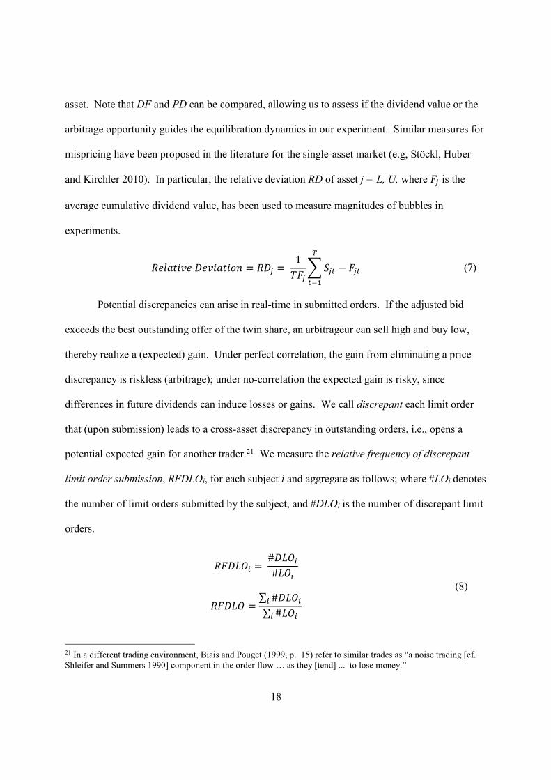
asset. Note that DF and PD can be compared, allowing us to assess if the dividend value or the
arbitrage opportunity guides the equilibration dynamics in our experiment. Similar measures for
mispricing have been proposed in the literature for the single-asset market (e.g, Stöckl, Huber
and Kirchler 2010). In particular, the relative deviation RD of asset j = L, U, where *� is the
average cumulative dividend value, has been used to measure magnitudes of bubbles in
experiments.
ABCD3EFB �BFED3EGH = A�� = 1�*� 9 ��' − *�'
=
'>? (7)
Potential discrepancies can arise in real-time in submitted orders. If the adjusted bid
exceeds the best outstanding offer of the twin share, an arbitrageur can sell high and buy low,
thereby realize a (expected) gain. Under perfect correlation, the gain from eliminating a price
discrepancy is riskless (arbitrage); under no-correlation the expected gain is risky, since
differences in future dividends can induce losses or gains. We call discrepant each limit order
that (upon submission) leads to a cross-asset discrepancy in outstanding orders, i.e., opens a
potential expected gain for another trader.21 We measure the relative frequency of discrepant
limit order submission, RFDLOi, for each subject i and aggregate as follows; where #LOi denotes
the number of limit orders submitted by the subject, and #DLOi is the number of discrepant limit
orders.
A*�IJK = #�IJK#IJK
A*�IJ = ∑ #�IJKK∑ #IJKK
(8)
21 In a different trading environment, Biais and Pouget (1999, p. 15) refer to similar trades as “a noise trading [cf. Shleifer and Summers 1990] component in the order flow … as they [tend] ... to lose money.”

19
We measure a trader’s aptitude is measured by the reverse of the frequency of submitting
a discrepant limit order, (1 - RFDLOi). The trader’s aptitude is therefore high if RFDLOi is small
and vice versa.
Our empirical measure of acuity is the individual’s CRT score, i.e., the number of correct
answers in the pre-market cognitive reflection task (Frederick 2005). Recent results in single-
asset market experiments have shown systematic effects of CRT scores (Corgnet et al. 2015,
Akiyama, Hanaki, and Ishikawa 2013; Breaban and Noussair 2014, Noussair et al. 2016). Below,
we also measure the effect of gender and risk aversion (as elicited in the investment game) on
our mispricing measures (4) – (8). Recent research from experimental single-asset markets
suggests that price levels may be lower if the level of risk aversion increases (Breaban and
Noussair 2014) and also if the share of female traders increases (Eckel and Füllbrunn 2015).
3.B. Testable Hypotheses
With measures (4) – (8) at hand we next formulate our testable hypotheses. Our most efficient
theoretical benchmark (which is standard in the experimental studies that apply the Smith et al.
1988 design, but is unlikely to obtain with inexperienced subjects in the laboratory) requires
prices to be equal to risk-neutral fundamental dividend values.
Hypothesis 0 (Risk-neutral pricing): There will be no deviations of prices from fundamentals in
either share class, i.e., �* = 0.
In line with the literature, we also look at a weak form of Hypothesis 0, that is, we
investigate if the RD measure is equal to zero on average. Risk-neutral pricing would require
that the price equals the fundamental dividend value in each period. In fact, risk-neutral pricing
is a sufficient (but not necessary) condition for obtaining MM invariance (Modigliani and Miller

20
1958). Indeed, previous experimental evidence (Palan 2013) shows that pricing deviations from
fundamental dividend value can be expected to occur in experimental asset markets in both
directions from above and below. This evidence does not invalidate the MM law of arbitrage-
free pricing. For arbitrage-free pricing and the MM theorem we require that our L-share and U-
share are priced at parity, which is indeed a much weaker requirement than risk-neutral
equilibrium pricing.
Hypothesis 1A (MM invariance theorem): The adjusted market values of L-shares and U-shares
will be the same, i.e., ∆'= 0. 1B (No cross-asset price discrepancy): 8� = 0. 1C (No discrepant
orders): A*�IJ = 0.
Hypothesis 1A requires that an L-share and a U-share (adjusted for fundamentals) are
priced the same on average. Hypothesis 1B (which implies 1A) requires that eventual deviations
from fundamentals occur simultaneously and equally in both shares. Hence, we investigate three
levels of market efficiency; the first is based on the absence of differences from parity pricing on
average (H1A), the second is based on the absence of price discrepancies (H1B) and discrepant
orders (H1C), and the third requires that prices coincide with risk-neutral dividend values (H0).
These levels of market efficiency are tested in two treatment dimensions. First, we
consider perfect correlation where elimination of pricing discrepancies is riskless, since dividend
streams differ by a constant and can be arbitraged. Second, we consider the case of no
correlation, where elimination of pricing discrepancies is risky because dividends are
independent of each other. Since the L-share and the U-share have identical idiosyncratic risks
in both treatments, and based on earlier evidence that suggests insensitivity of behavior to
changes in return correlations (e.g., Kroll et al. 1988), one might expect no treatment effect in
the laboratory. However, the MM arbitrage result concerns only the relative pricing of two

21
assets, not the absolute level of their prices. Thus, it could be that both assets are mispriced in
absolute terms but their relative pricing is aligned, so there is no arbitrage opportunity. Given
that mispricing has been frequently observed in the considered experimental design, we expected
to observe some mispricing in our experiments and state the following testable hypothesis:
Hypothesis 2. (Hedging effect): The cross-asset price discrepancy (PD) will be larger in the no-
correlation treatment than in the perfect-correlation treatment.
The hypothesis suggests that markets can eliminate some price discrepancies in the
absence of risk even without a dedicated (automatic) arbitrageur, and so decrease the magnitude
of the PD-value in the presence of perfect correlation. Hypothesis 2 suggests the relative validity
of MM invariance under perfect correlation, relative to no correlation.
Anticipating from experimental evidence of mispricing in early markets (e.g., Smith et al.
1988, Dufwenberg et al. 2005), we expect a decrease of mispricing in our consecutive markets.
Hypothesis 3. (Experience effect): The cross-asset price discrepancy (PD), the deviation from
fundamental dividend value (DF), and the relative frequency of discrepant orders (RFDLO) will
decrease over time (in consecutive markets).
It is an oft-cited conjecture that smart investors eliminate mispricing in the market (see
e.g., Shleifer 2000). Although our design has no dedicated arbitrageur, we can nevertheless
address the predictive power of this argument in our data. We compare the magnitude of price
discrepancies vis-à-vis characteristics of market participants, suggesting a relationship between
acuity and aptitude of traders.
Hypothesis 4. (Smart trader effect) The cross-asset price discrepancy (PD), deviation from
fundamental dividend value (DF), and the relative frequency of discrepant orders (RFDLO) will
decrease with the market participants’ degree of measured acuity.

22
We are also interested in the equilibration dynamics of the market. When a price
discrepancy arises, that is, when the L-share and the U-share are mispriced relative to one
another, at least one share (if not both) are mispriced vis-à-vis the fundamental dividend value.
Exploitation of this mispricing leads to expected gains. We anticipate that the more profitable
trade will happen first in both treatments. The more profitable trade is the one whose expected
return is the larger one within the discrepancy pair. It can be either a long or short position.
Moreover, we also expect, especially in the perfect-correlation treatment (but also in the no-
correlation treatment), that subjects exploit price discrepancies by simultaneously taking long
and short positions, thus eliminating the discrepancy and booking an arbitrage (expected) gain.
The latter behavior is what MM suggest in their arbitrage proof.
Hypothesis 5A (Equilibration dynamics) Where cross-asset price discrepancy arises the higher
expected return twin share trades first. 5B (Asset swap/MM arbitrage) The price discrepancy is
exploited through (almost) simultaneous trade in the twin shares by the same subject.
Finally, we investigate the effect of return correlation on individual portfolio
diversification. Portfolio diversification reduces fluctuations in portfolio returns when
correlations are smaller. Financial economics suggests that people are averse to return volatility.
Therefore, we conjecture that the difference between the number of U-shares and L-shares is
smaller in the no-correlation treatment than in the perfect correlation treatment.22 Let 1#K' and
1$K' be the number of U-shares and L-shares in the portfolio of subject i at the end of period t,
and N1K' = |1#K' − 1$K'| is the absolute difference of the two numbers. We compare the average
22 Our measure of diversification is very simple. We look at individual deviations from the market portfolio. Investor subjects are perfectly diversified in our design if they hold an equal number of L-shares and U-shares. Different from the no-correlation treatment, return volatility does not decrease with increased diversification in the perfect-correlation treatment.

23
individual portfolio diversification over subjects and periods, which we denote by dZ(ρLU),
across markets and treatments.
Hypothesis 6 (individual portfolio diversification) Subjects are more diversified in the no-
correlation treatment (0) than in the perfect correlation treatment (1), N1607 ≤ N1617.
4. Results
In total, 174 students participated, earning an average of $50 in 3 hours. Each participated in
only one session. We have 12 sessions in the perfect-correlation treatment and eight sessions in
the no-correlation treatment.23 Each session is comprised of four consecutive markets.24
4.A. MM invariance theorem
Observation 1. L-share and U-share prices are close to parity and in line with the MM
invariance theorem in the perfect-correlation treatment. U-share prices are above parity
in the no-correlation treatment.
Support. In Figure 1, we see the difference of L-share and U-share prices relative to parity for
each market, period, and treatment, aggregated separately over the 12 sessions of the perfect-
correlation treatment and the eight sessions of the no-correlation treatment. In the case of a
23 We do not have the same number of sessions across treatments. Unfortunately, we discovered a problem in the software after conducting the first four sessions. Owing to this problem, the L-share holders received no cash dividend; instead, both L-share and U-share dividends were distributed to U-share holders. Due to logistical and timing problems, we were unable to book the lab to conduct these four sessions and so have only eight cohorts in the no-correlation treatment rather the planned 12 cohorts. 24 In the fourth market of one session of the perfect-correlation treatment, one subject submitted an obviously erroneous bid (instead of an asking price) for $20 on the L-share worth $0.24 that led to a transaction. We have eliminated the period from the data as the transaction impacts our average estimates. In the second market of the two other perfect-correlation sessions, the data for period 10 are missing (due to a server crash). One session of the perfect-correlation treatment and two sessions of the no-correlation treatments had only seven participants.

24
missing price of L-share or U-share, the period in the session is treated as a missing
observation.25 The prices in the perfect-correlation treatment are close to parity, whereas the
prices in the no-correlation treatment are above parity. In view of our theoretical discussion, we
note that no direction of deviation could be predicted. In contrast, the data suggest that the
deviation of relative market valuation has a direction, indicating a relatively higher price for the
U-share than the L-share.26 Below we further investigate the pattern.
Figure 1. Evolution of relative difference from price-parity of L-shares and U-shares ∆O The abscissa shows the periods 1 to 10 and represents price parity between L-share and U-share prices.
The ordinate indicates the relative difference from parity from -0.2 to 0.6. Each chart represents the
relative difference from price-parity for one market of 10 periods; markets 1-4 are represented top left,
top right, bottom left, and bottom right.
25 On average we have 11% and 5% missing observations in the perfect-correlation and no-correlation treatments, respectively. 26 In this context the dividend puzzle comes to mind (DeAngelo and DeAngelo 2006), that is, the empirical observation that the market value of dividend-paying stock is higher than of zero dividend stock. Whereas the U-share always pays a positive dividend, the L-share indeed pays a zero dividend 25% of the time.
-0.20
0.00
0.20
0.40
0.60
1 2 3 4 5 6 7 8 9 10
Perfect correlation Market 1 No correlation
-0.20
0.00
0.20
0.40
0.60
1 2 3 4 5 6 7 8 9 10
Perfect correlation Market 2 No correlation
-0.20
0.00
0.20
0.40
0.60
1 2 3 4 5 6 7 8 9 10
Perfect correlation Market 3 No correlation
-0.20
0.00
0.20
0.40
0.60
1 2 3 4 5 6 7 8 9 10
Perfect correlation Market 4 No correlation
25
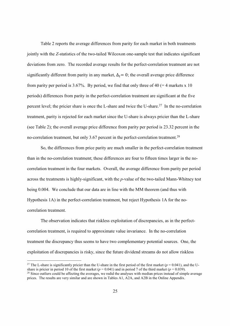
Table 2 reports the average differences from parity for each market in both treatments
jointly with the Z-statistics of the two-tailed Wilcoxon one-sample test that indicates significant
deviations from zero. The recorded average results for the perfect-correlation treatment are not
significantly different from parity in any market, ∆'= 0; the overall average price difference
from parity per period is 3.67%. By period, we find that only three of 40 (= 4 markets x 10
periods) differences from parity in the perfect-correlation treatment are significant at the five
percent level; the pricier share is once the L-share and twice the U-share.27 In the no-correlation
treatment, parity is rejected for each market since the U-share is always pricier than the L-share
(see Table 2); the overall average price difference from parity per period is 23.32 percent in the
no-correlation treatment, but only 3.67 percent in the perfect-correlation treatment.28
So, the differences from price parity are much smaller in the perfect-correlation treatment
than in the no-correlation treatment; these differences are four to fifteen times larger in the no-
correlation treatment in the four markets. Overall, the average difference from parity per period
across the treatments is highly-significant, with the p-value of the two-tailed Mann-Whitney test
being 0.004. We conclude that our data are in line with the MM theorem (and thus with
Hypothesis 1A) in the perfect-correlation treatment, but reject Hypothesis 1A for the no-
correlation treatment.
The observation indicates that riskless exploitation of discrepancies, as in the perfect-
correlation treatment, is required to approximate value invariance. In the no-correlation
treatment the discrepancy thus seems to have two complementary potential sources. One, the
exploitation of discrepancies is risky, since the future dividend streams do not allow riskless
27 The L-share is significantly pricier than the U-share in the first period of the first market (p = 0.041), and the U-share is pricier in period 10 of the first market (p = 0.041) and in period 7 of the third market (p = 0.039). 28 Since outliers could be affecting the averages, we redid the analyses with median prices instead of simple average prices. The results are very similar and are shown in Tables A1, A2A, and A2B in the Online Appendix.

26
arbitrage. The risky exploitation of a discrepancy requires a risk premium, implying larger
discrepancies. Second, the market discounts the U-share less than the L-share. In principle, this
could indicate the existence of a certainty effect in the data (Kahneman and Tversky 1979)
concerning non-zero payoffs: while the U-share dividend is strictly positive by definition, the L-
share dividend can be zero in every period. However, our follow-up treatments (see below) do
not find supporting evidence, and so the reason for this behavior is not completely clear to us.
Table 2. Average difference from parity ∆ in percent
The table records the difference from parity (4) averaged over ten periods and all
sessions for each market and both treatment. The first column records the averages
for the perfect correlation treatment and the second column for the no-correlation
treatment. The bottom line shows the average difference from parity over all periods.
Asterisks indicate significant differences from parity measured by the two tailed, one-
sample Wilcoxon signed-ranks test. The last column shows the p-value resulting from
the two tailed, two-sample Mann-Whitney test. Z-statistics are recorded in brackets.
Significant differences are indicated; ***p < 0.01, **p < 0.05, *p < 0.10.
Treatment
Perfect correlation (n = 12)
No correlation (n = 8)
Mann-Whitney test (between
treatments), p-value, [Z-
statistic]
Market 1 6.98
[0.39] 27.72**
[2.24] 0.031** [2.16]
Market 2 1.72
[0.04] 29.92**
[2.52] 0.001*** [3.28]
Market 3 3.49
[1.49] 17.94**
[2.10] 0.165 [1.39]
Market 4 2.62
[1.26] 14.49**
[2.52] 0.064* [1.85]
Average 3.67
[1.53] 22.52**
[2.52] 0.006*** [2.78]
4.B. Pricing discrepancies and deviation from fundamentals
Observation 2. Absolute difference from parity (PD), the deviation from fundamentals
(DF) and the relative frequency of discrepant orders (RFDLO) are reduced in the
perfect-correlation treatment relative to the no-correlation treatment.

27
Support. The data in Table 3A, Table 3B and Table 3C record the averages of PD-value, DF-
value and RFDLO by treatment, respectively.29 From Table 3A we see that by buying the lower-
priced share and selling the higher-priced twin share (both at the average price in a randomly-
determined period), the average riskless return would be 23 percent of the trading value in the
first market of the perfect-correlation treatment. This number is relatively large if compared to
the second market, where the average PD-value drops to one half of the first market.30 However,
the amount of the decrease is rather small relative to the first market in the no-correlation
treatment. As indicated by the one-tailed Mann-Whitney test recorded in the table, the PD-value
is larger overall (at the 10% significance level) than in the no-correlation treatment.
We see in Table 3B that the results for the DF-value point in the same direction. The
overall average absolute deviation from the fundamental dividend value is 19.13 percent in the
perfect-correlation treatment and 27.39 percent in the no-correlation treatment. Nevertheless, the
differences between the two treatments are only significant (at the five percent level) for the
second market. The results suggest that pricing relative to fundamentals is (relatively)
independent of whether there are perfect arbitrage conditions. In line with the literature, both
treatments trend towards the fundamental dividend value with repetition. We conclude that the
data rather support than reject Hypothesis 2 and Observation 2 vis-à-vis the PD and DF values,
particularly for Market 2, although the evidence is not statistically-significant for all markets.
Table 3C records the average number of discrepant orders relative to the submitted orders
in a market. The overall average number of discrepant limit orders is 5.70 percent in the perfect-
29 These values have been computed according to equations (5), (6) and (8). A missing average price of L-share or U-share in a certain period is treated as a missing observation in the corresponding session. The minimum PD-value overall markets and the first quartile in the perfect-correlation treatment is 1.1 percent and 8.4 percent, and in the no-correlation treatment 5.0 percent and 13.7 percent, respectively. 30 The decrease from the first to the second market is significant at the one percent level (Z = 2.353, p = 0.009, one-tailed Mann-Whitney test, n = 12).

28
correlation treatment and 10.22 percent in the no-correlation treatment. The differences are
significant across treatments.
In terms of absolute numbers of arbitrage and mispricing, Hypothesis 0 and Hypothesis
1B and 1C must be rejected given that no session and market involves a zero DF-value, a zero
PD-value, or zero RFDLO-value.
Table 3A: Average absolute deviation from parity PD in percent
The table records the price discrepancy (5) for the ten market periods averaged over all
sessions for each market and treatment. The bottom lines show the average price
discrepancy over all periods, and the one-tailed Page trend test that checks for a
significant decline in repeated markets. The last column shows the p-value resulting
from the two tailed, two-sample Mann-Whitney test. Z-statistics are recorded in
brackets. Significant differences are indicated; ***p < 0.01, **p < 0.05, *p < 0.10.
^One-tailed tests.
Perfect correlation
(n1 = 12)
No correlation
(n2 = 8)
Mann-Whitney test
(between treatments),
p-value, [Z-statistic]^
Market 1 24.59 39.52 0.316
[1.00]
Market 2 15.25 30.36 0.045**
[2.01]
Market 3 15.87 22.34 0.32
[1.00]
Market 4 21.65 17.35 0.758
[-0.31]
Total 19.34 27.39 0.563
[0.58]
p-value (one-tailed Page trend test)^
0.159
[-1.00]
0.011**
[-2.30]
29
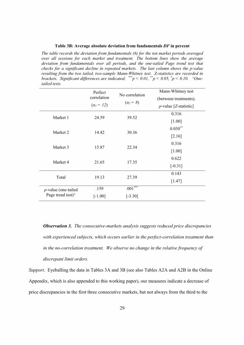
Table 3B: Average absolute deviation from fundamentals DF in percent
The table records the deviation from fundamentals (6) for the ten market periods averaged
over all sessions for each market and treatment. The bottom lines show the average
deviation from fundamentals over all periods, and the one-tailed Page trend test that
checks for a significant decline in repeated markets. The last column shows the p-value
resulting from the two tailed, two-sample Mann-Whitney test. Z-statistics are recorded in
brackets. Significant differences are indicated; ***p < 0.01, **p < 0.05, *p < 0.10. ^One-
tailed tests.
Perfect correlation
(n1 = 12)
No correlation
(n2 = 8)
Mann-Whitney test
(between treatments),
p-value [Z-statistic]
Market 1 24.59 39.52 0.316
[1.00]
Market 2 14.42 30.36 0.030**
[2.16]
Market 3 15.87 22.34 0.316
[1.00]
Market 4 21.65 17.35 0.622
[-0.31]
Total 19.13 27.39 0.143
[1.47]
p-value (one-tailed Page trend test)^
.159
[-1.00]
.001***
[-3.30]
Observation 3. The consecutive-markets analysis suggests reduced price discrepancies
with experienced subjects, which occurs earlier in the perfect-correlation treatment than
in the no-correlation treatment. We observe no change in the relative frequency of
discrepant limit orders.
Support. Eyeballing the data in Tables 3A and 3B (see also Tables A2A and A2B in the Online
Appendix, which is also appended to this working paper), our measures indicate a decrease of
price discrepancies in the first three consecutive markets, but not always from the third to the

30
fourth market. The non-parametric Page trend test (n = 12, k = 4) as reported in the bottom line
of Table 3A suggests no significant decrease of the PD-value over four markets in the perfect-
correlation treatment;31 on the other hand, the test results reported in Table 3B do indicate a
decrease for the deviation from fundamentals that is significant at the 10 percent level. The
results of the one-tailed Page test are significant at the five percent level for the no-correlation
treatment, indicating a reduction over time of the PD-value and DF-value.
Table 3C: Average rel. freq. of discrepant limit orders RFDLO in percent
The table records the frequency of discrepant limit orders relative to submitted limit orders
(8) by session for each market and treatment. The bottom lines show the average relative
frequency of discrepant limit orders over all periods, and the one-tailed Page trend test that
checks for a significant decline in repeated markets. The last column shows the p-value
resulting from the two tailed, two-sample Mann-Whitney test. Z-statistics are recorded in
brackets. Significant differences are indicated; ***p < 0.01, **p < 0.05, *p < 0.10. ^One-
tailed tests.
Perfect
correlation (n1 = 12)
No correlation (n2 = 8)
Mann-Whitney test (between treatments), p-value, [Z-statistic]
Market 1 6.76 10.90 0.190 [1.31]
Market 2 4.96 10.58 0.123 [1.54]
Market 3 4.81 9.61 0.105 [1.62]
Market 4 5.51 9.81 0.037** [2.08]
Total 5.51 10.23 0.045** [2.01]
p-value (one-tailed Page trend test)^
0.242 [-.70]
0.460 [-.10]
We have no significant evidence for the continuous convergence to the theoretical
predictions over all the four markets in the perfect-correlation treatment, since convergence
31 In the fourth market in some sessions, subjects push prices to irrationally high levels in late periods. Even if these data points were ignored, however, the price discrepancies would not be reduced from the level of Market 3. That said, the reported p-value of the Page test suggests that a declining PD-value in the perfect-correlation treatment would then be significant at the five percent level.

31
seems to occur all at once from the first to second market, after which deviations remain at the
same level until the end. Thus, the perfect-correlation treatment exhibits a significant decline at
the five percent level in PD-value and DF-value between the first and the second markets, but
not between any other consecutive markets.32 On the other hand, the main decline in the no-
correlation treatment occurs from Market 2 to Market 3.33 Thus, the data suggest a more rapid
adjustment to the theoretical benchmarks in the perfect-correlation treatment, i.e., when an
exploitation of price discrepancies is riskless.
Table 3C suggests no decline of the RFDLO by the one-tailed Page test.
Observation 4. The differences between PD and DF suggest that pricing discrepancies
are a more focal driver of behavior than the deviation from fundamentals in the perfect-
correlation treatment when compared to the no-correlation treatment.
Support. Comparing Tables 3A and 3B, the PD-values are smaller than the DF-values for each
market of the perfect-correlation treatment and larger for each market of the no-correlation
treatment.34 The average difference between PD-values and DF-values over all markets is -0.029
in the perfect-correlation treatment and 0.017 in the no-correlation treatment. The difference
between treatments is significant; per the one-tailed Mann Whitney two-sample test, the p-value
is 0.071. Hence, the data suggest that the pricing vis-à-vis the other asset is focal in the perfect-
32 The p-values of the one-tailed Wilcoxon signed ranks test that suggest a decline between first and second market are as follows; PD-value (p = 0.010, Z = 2.316), and DF-value (p = 0.009, Z = 2.353). 33 The PD-value (p = 0.034, Z = 1.820) and the DF-value (p = 0.034, Z = 1.820) decrease significantly at the five percent level between Market 2 and Market 3 only, but not between Market 1 and Market 2 (p = 0.116, Z = 1.193), (p = 0.104, Z = 1.260). 34 On average over all markets, the difference between PD-value and DF-value is significantly different from zero in the perfect correlation treatment. Per the two-tailed Wilcoxon signed ranks test, the p-value is 0.0995. In the no-correlation treatment we have no significant differences between PD-value and DF-value.

32
correlation treatment compared with the no-correlation treatment. The results reported in section
5.5, where we examine at the equilibrating dynamics, underline this effect.
4.C. Bubble magnitude
Following the standard line of experimental asset-market research, we report the standard
measure of bubble magnitude RD (relative deviation) for our treatments by asset. Given that the
literature on the single-asset market has shown that mispricing of assets frequently occurs (Palan
2013), we have a surprising result:
Observation 5. a) Asset prices average close to the dividend value in the perfect-
correlation treatment. The RD measures of the L-share and the U-share are near zero. b)
The price of the U-share in the no-correlation treatment exceeds the dividend value, i.e.,
the RD measure is significantly positive, while the average price of the L-share is close to
the expected dividend value.
Support. Figure 2 and Figure 3 show the average price trajectories for all sessions and overall.
Table 4 records for each market (by treatment) the standard measure of mispricing the relative
deviation RD measure for the L-share and the U-share (and their differences) as described in
section 4 and as commonly applied in the literature (Stöckl, Huber and Kirchler 2010). The
figure illustrates observations 5a) and 5b). The overall average RD measures are -0.041 and
0.171 for the L-share and the U-share in the no-correlation treatment and -0.025 and 0.023 for
the perfect-correlation treatment. The deviations from expected cumulative dividend value are
statistically significant for the U-share in the no-correlation treatment, where the RD measure is
significantly different from (i.e., larger than) zero for each market and overall. In the perfect-

33
Figure 2. Average prices in markets 1-4 (left to right, top to bottom) of the Perfect Correlation
treatment
The trajectories of all 12 cohorts are displayed for both assets L-share and U-share, and the average for
each asset is indicated in bold. The dividend values are displayed by cascading short horizontal lines,
but here they are almost covered by the lines that indicate the overall averages. The ordinate indicates
the average prices from 0 to 700, and the abscissa the periods 1 to 10.
Figure 3. Avg prices in markets 1-4 (left to right, top to bottom) of the No Correlation treatment
The trajectories of all 8 cohorts are displayed for both assets L-share and U-share, and the average for
each asset is indicated in bold. The dividend values are displayed by cascading short horizontal lines,
which are well visible for the U-share. They are almost covered for the L-share by the lines that indicate
the overall averages. The ordinate indicates the average prices from 0 to 700, and the abscissa the
periods 1 to 10.
0
100
200
300
400
500
600
700
1 2 3 4 5 6 7 8 9 10
0
100
200
300
400
500
600
700
1 2 3 4 5 6 7 8 9 10
0
100
200
300
400
500
600
700
1 2 3 4 5 6 7 8 9 10
0
100
200
300
400
500
600
700
1 2 3 4 5 6 7 8 9 10
0
100
200
300
400
500
600
700
1 2 3 4 5 6 7 8 9 10
0
100
200
300
400
500
600
700
1 2 3 4 5 6 7 8 9 10
0
100
200
300
400
500
600
700
1 2 3 4 5 6 7 8 9 10
0
100
200
300
400
500
600
700
1 2 3 4 5 6 7 8 9 10

34
Table 4: Average RD measure and difference between shares in percent The table records the average relative deviation (7) for each market, assets L, and U, and
treatment. The bottom line shows the average over all markets. The third and sixth columns
show the differences between RD values of assets L and U. The RD-values and their
differences between assets L and U are tested. Z-statistics are recorded in brackets.
Significant differences from zero resulting from the two tailed, one-sample Wilcoxon signed
ranks test are indicated; ***p < 0.01, **p < 0.05, *p < 0.10.
Perfect correlation (n1 = 12)
No correlation (n0= 8)
A�$ A�# A�#-A�$ A�$ A�# A�#-A�$ Market 1 2.80
[0.31]
9.48 [1.02]
6.68 [0.16]
0.24 [0.56]
22.13** [2.38]
21.90* [1.68]
Market 2 -5.53 [-1.10]
-0.01 [-0.39]
4.92 [1.02]
-5.03 [0.14]
22.49*** [2.52]
27.52*** [2.52]
Market 3 -11.00** [-2.28]
-2.19 [-0.83]
8.82** [2.28]
-5.91 [-0.21]
12.57** [2.24]
18.48* [1.40]
Market 4 3.68 [-0.24]
2.44 [0.39]
-1.24 [0.24]
-5.54 [0.14]
11.40** [2.38]
16.94** [2.38]
Total avg.
-2.51 [-.78]
2.28
[1.26] 4.79
[0.94] -4.06
[0.14] 17.15**
[2.52] 21.21*** [2.52]
correlation treatment, the overall RD measure is not significantly different from zero; a
significant (negative) RD measure is only recorded for the L-share in market 3.
Comparing across assets, we find that the RD measures of the L-share and the U-share
are significantly different in the no-correlation treatment; in the perfect-correlation treatment
there are no significant differences between RD measures of the L-share and the U-share.35 If we
compare RD measures between treatments and shares, we find that only the RD measure of the
U-share in the no-correlation treatment is significantly different from (i.e., larger than) the
others.36 This misbehavior of the U-share is puzzling and seems to mainly drive the reported
violation of parity pricing in the no-correlation treatment. The Spearman rank correlation
35 Based on the two-tailed Wilcoxon signed ranks test results we reject the null hypothesis of equal RD measures between L-share and U-share for the no-correlation treatment; the p-value is 0.012. In the perfect-correlation treatment the p-value is 0.347 and so we conclude that the RD measures do no significantly differ across assets. 36 The p-values of the two-tailed Mann-Whitney two-sample test (on the total average) are as follows; between U-shares (p = 0.000), between L-shares (0.227); between the difference of U-share and L-share (0.007).

35
between the A�# and ∆ are 0.168 and 0.810 in the perfect-correlation and the no-correlation
treatments, respectively; the latter indicates a significant correlation (p-value is 0.015) whereas
the former does not (p-value is 0.602).37 The question here is why the deviations occur in the U-
share of the no-correlation treatment and not in the L-share. Below we investigate this finding
further by looking at the market behavior and at the valuations of the L-share and the U-share in
the single-asset market.
4.D. Smart traders
Observation 6. Individual performance (i.e. payoff) correlates with measured acuity.
Support. Table 5A reports regression results. We use the subject’s average payoff over the four
markets as the individual-performance measure. As stated above, we measure individual acuity
by the CRT score, i.e., the individual’s number of correct answers. The average CRT score in
our sample was 0.97.38 As a risk-aversion measure we use the individual percentage allocation
to the safe asset in the investment game; the average allocation was 60 percent. Finally, we
consider gender, assigning value one for a female investor and zero otherwise. The share of
females is 49 percent in our subject pool (see subject-pool composition details in Table A3 in the
Online Appendix which is also appended to this paper).39
37 Note also that the differences in RD-values between L-share and U-share and deviations from parity are highly correlated. The Spearman rank correlation coefficient is 0.862 on the overall sample, which is significant at any commonly accepted significance level (p-value is 0.000). 38 This is a bit lower than average (see Frederick (2005), who finds an average in a very large sample of 1.24). One might have expected a better result here for CRT because of incentivization. The lower number could have resulted from the fact that our subjects were time constrained whereas Frederick’s were not. 39 As in many previous studies (see Charness and Gneezy, 2012), our measure finds that females are significantly more financially risk averse than males (Z = 2.366, p = 0.018, two-tailed test). In line with the results of Frederick (2005), we also find that males in our sample have significantly higher CRT scores (Z = 3.838, p < 0.001, two-tailed test).

36
Table 5A. Regression results
The first two columns record the outcomes of the cluster regression with robust standard errors of
the within-group individual payoff and aptitude (the reciprocal of the relative frequency of a limit
order that opens up an arbitrage opportunity) on the individual CRT-score (8), Risk Aversion, and
FEM gender dummy. The other columns record the OLS regression results of measures (4)-(8) on
the group average of the individual measures. The results of two-tailed t-tests are indicated [Z-
statistics in brackets]; ***p < 0.01, **p < 0.05, *p ≤ 0.10.
Variable Payoffi
1-RFDLOi ∆ PD DF RFDLO A�#
Intercept 2717.9***
[22.8] 0.976*** [138.9]
0.925** [0.02]
0.949* [2.04]
0.811** [2.73]
0.345*** [3.42]
0.514** [2.77]
CRT-score 161.8*** [3.67]
0.005** [2.07]
-0.643*** [-3.84]
-0.69*** [-3.10]
-0.579*** [-4.06]
-0.142*** [-2.98]
-0.30*** [-3.34]
Female -241.0*** [-2.90]
0.008 [1.31]
-0.198 [-1.20]
-0.164 [-0.75]
0.114 [0.81]
-0.086*
[-1.82] -0.058
[-0.66]
Risk aversion -0.76
[-0.59] -0.000 [-0.52]
0.001 [0.12]
0.002 [0.29]
-0.000 [-0.09]
-0.001
[-0.75] -0.000
[-0.12]
perf. correlation treatment dummy
-0.824***
[-3.10] -0.81**
[-2.29] -0.506**
[-2.23] -0.154*
[-2.04] -0.369**
[-2.60]
CRT-score x treatment dummy
0.646**
[2.42] 0.697*
[1.95] 0.427*
[1.87] 0.102
[1.35] 0.218
[1.53]
#obs. 174 174 20 20 20 20 20
#clusters 20 20
R-squared .125 .039 .653 .484 .640 .591 .728
The outcomes of the ordinary-least-square regression of the individual performance
measure on the CRT score, Female, and Risk aversion are recorded in the first column of Table
5A. The OLS regressions use clustered standard errors (clustered by independent session). As
indicated, the CRT score is a significant determinant of the individual performance in this

37
regression, but gender and the risk-aversion measure are not significant. We find no significant
differences across treatments.40 The evidence clearly supports Observation 6.
Instead of measuring performance by payoff as in Observation 6, we can measure
performance by the number of bad decisions in trading. As explained above, we compute the
ratio of the number of discrepant limit orders to total limit orders, RFDLOi. This ratio is next
compared to the individual CRT score.
Observation 7. The trader’s aptitude is correlated with the measured individual acuity.
Support. The trader’s aptitude is reversely related to the relative frequency of submissions of
discrepant limit orders to the trader’s total number of submitted limit orders, (1 - RFDLOi). As
characterized above, a discrepant limit order offers an arbitrageur’s opportunity to realize a
(expected) gain by swapping assets. The measured trader’s aptitude is regressed on individual
characteristics. The second column of Table 5A records OLS regressions with clustered standard
errors (clustered by independent cohort). We find that the individual acuity measured by the
CRT score thus explains much of the bidding data, supporting Observation 7.
Observation 8. When there is high overall trader acuity, price discrepancies are smaller,
fewer discrepant orders are submitted, and the price of assets is closer to parity.
Support. In Table 5A we also record four OLS regressions of our measures (4)-(6), (8) on the
group aggregate personal measures. In these regressions the average CRT score always shows
up significantly. The difference of price from parity, deviation from fundamentals, and price
40 The two-tailed Mann-Whitney test between treatments returns the following p-values on the individual-level data, 0.559 (risk aversion), 0.809 (Female) and 0.987 (CRT score), and similar p-value results on the session-level data, 0.165 (risk aversion), 0.754 (Female), and 0.529 (CRT score).

38
discrepancy as well as the relative frequency of discrepant orders decrease in markets with
overall high trader acuity. In the regression, we also control for treatment effects of CRT. As
the interaction with the treatment dummy indicates, the CRT-effect is strong for the no-
correlation treatment. In Table 5B we report Spearman rank-correlation coefficients of the CRT
score with our measures of market efficiency. The coefficients also hint at a treatment effect.
The correlation coefficients usually have the same sign in both treatments, but the magnitude of
the coefficients is larger for the no-correlation treatment. The reported test results indicate that
the reported CRT effects could be driven by the no-correlation treatment. So, as for Hypothesis
4 and Observation 8, we conclude that acuity could actually affect reduction of price discrepancy;
however, potential discrepancies do not disappear completely.
Table 5B. Spearman rank correlation coefficient with CRT score
Correlation coefficients are reported for CRT effect in measures (4)-(8)
for each treatment separately. The results of two-tailed Spearman rank
correlation test are indicated; ***p < 0.01, **p < 0.05, *p ≤ 0.10
∆ PD DF RFDLO A�#
Perfect correlation
treatment, n = 12 -0.236 -0.271 -0.236 -0.268 -0.168
No-correlation treatment, n = 8
-0.732** -0.634* -0.634* -0.683* -0.927***
Observation 9. When there is low overall trader acuity, or low trader aptitude, U-share
prices exceed fundamentals in the no-correlation treatment. There is no significant
impact of trader acuity, risk aversion, or gender composition with either the L-share in
the no-correlation treatment or either share in the perfect-correlation treatment.
Support. In the last column of Table 5A, we record a simple OLS regression of our acuity
measure on the group aggregate personal measures for the no-correlation treatment. The result

39
shows that the RD measure increases with decreasing CRT-score. This effect is present in the U-
share of the no-correlation treatment only, as the effect in L-share and in the perfect-correlation
treatment is not significantly different from zero (see also Table 5B).41
4.E. Equilibrating dynamics
Observation 10. The relative frequency of discrepancies in the perfect-correlation
treatment is lower than in the no-correlation treatment. Where a pricing discrepancy
arises, subjects trade the high-expected-return twin share first rather than the less
profitable one. Individual subjects rarely exploit pricing discrepancies by asset swaps.
Support. As reported in Table 3C, on average 5.5 percent and 10.23 percent of all submitted
orders lead to discrepancies in the order book for the perfect-correlation treatment and the no-
correlation treatment.42 We observe equilibrating dynamics as discussed in Section 4. When a
discrepancy arises, a trade in one twin share typically leads to a higher expected return than a
trade in the other.
As recorded in Table 6, the relative frequencies at which the high-return trade is enacted
first are 0.886 and 0.916 in the perfect-correlation treatment and the no-correlation treatment.
The results of the Wilcoxon signed-ranks test show that the equilibration dynamics work as
suggested above, thus confirming Hypothesis 5A. It is significantly more likely that a
41 A significant correlation of RDU measure and CRT-score is only notable in the no-correlation treatment. Conducting an OLS regression (with CRT as the only explanatory variable) separately for each treatment results in p-values of 0.318 (perfect correlation) and 0.026 (no correlation) for the slope of the CRT score. The other explanatory variables including our measure of risk aversion and the gender share have no significant impact on any RD in the two treatments. 42 The difference between treatments is in the expected direction, and significant as reported above. The share of discrepancies and the PD-value in a session are highly correlated. The OLS regression (on the level of the independent session) of the RFDLO-value on the PD-value indicates a significantly positive slope (z-statistic of 2.43, i.e., p = 0.026) and a determination coefficient of 0.25. When a discrepancy arises, the median response time is 4 seconds.

40
transaction occurs first in the high-expected-return twin-share, thus eliminating the price
discrepancy without necessarily booking an arbitrage gain. So prices are pushed in the direction
of fundamental dividend value.43
Table 6: Equilibrating dynamics: relative frequency of market orders in the
high-expected-return share of given discrepancy
The Table records the relative frequency in percent by which the market trades the
more-profitable rather than the less-profitable share when a discrepancy arises.
Significant differences per the one-tailed Wilcoxon signed-ranks tests are
indicated; ***p < 0.01, **p < 0.05, *p < 0.10. Numbers in brackets are z-statistics.
Perfect correlation (n1 = 12)
No correlation
(n2 = 8)
Two tailed Mann-Whitney test
(between treatments), p-value [Z-statistic]
Market 1 85.0*** [2.99]
95.8*** [2.52]
0.054** [2.47]
Market 2 88.4*** [3.07]
98.1*** [2.55]
0.086* [1.71]
Market 3 93.8*** [3.10]
81.8** [2.25]
0.332 [-0.97]
Market 4 87.0*** [3.07]
90.9*** [2.52]
0.586 [0.56]
Total 88.6*** [3.06]
91.7*** [2.52]
0.758 [0.31]
In fact, subjects rarely exploit the price discrepancy (as arbitrageurs would do) by selling
the relatively expensive twin share and simultaneously buying the cheap one. Such hedging
trades happen about 1% of the time when a discrepancy arises. Our hypothesis 5B is not
supported by the data; 99% of discrepancies were eliminated by independent trades in the market
rather than by individuals engaging in arbitrage; no arbitrageur subjects dominate the market.
We conclude that the described market equilibration dynamics imply a narrowing of the gap
between prices of twin shares in our treatments rather than high-skilled individual traders.
43 The effect is a bit stronger in the no-correlation treatment than in the perfect correlation treatment. However, equilibration dynamics are strong in both treatments. The difference is possibly related to the above-described fact that relative pricing is a more important driver of price behavior in the perfect correlation treatment than in the no-correlation treatment.

41
4.F. Individual portfolio diversification
Despite the fact that diversification can lower the return volatility in the no-correlation treatment,
but not in the perfect-correlation treatment, the average individual difference in subjects’
portfolios of L-shares and U-shares is 2 (= dZ) in each treatment. The difference in individual
portfolio diversification between treatments is close to zero.44 Hence, we have no evidence in
support of Hypothesis 6.
4.G. Summary of experimental results
We do not observe pricing of assets at fundamental dividend value, but we have support for
Hypothesis 1A (MM invariance theorem) in our perfect-correlation treatment, where exploitation
of a price discrepancy is riskless. This differs in relative terms when we compare the data to the
no-correlation treatment, where exploitation of price discrepancies across assets has risk.
Hypothesis 1B (no price discrepancy) is not supported in either of our treatments as price
discrepancies seem to persist. Under perfect correlation, however, adjustment to a level where
discrepancies stabilize is fast (achieved by the second market) whereas under no correlation
adjustment takes at least more time. Hypothesis 2 (hedging effect) is confirmed; the results on
price discrepancies of the perfect-correlation treatment are closer to the theoretical prediction
than those of the no-correlation treatment.
Support for Hypothesis 3 (experience effect) is no surprise; experienced subjects trade
closer to the theoretical predictions than inexperienced subjects. Nonetheless, unlike the results
of the single-asset market (Smith et al. 1988) our data do not suggest a complete convergence on
fundamental dividend values or vanishing price discrepancies in repeated markets. Moreover,
44 The p-value of the one-tailed Mann-Whitney between-sample tests is 0.47.

42
discrepant order submissions do not cease with repetition, as indicated by the stable relative
frequency of discrepant limit orders. We find some support for Hypothesis 4 (smart trader effect)
as our measure of aptitude increases in our measure of acuity and market mispricing decreases
with the measured level of acuity. To the extent that experience may substitute for initial acuity,
ours confirm other results in the experimental-asset-markets literature (Palan 2013).
Our data support our equilibration Hypothesis 5A. When a discrepancy arises, the more
profitable transaction is enacted first thus pushing price dynamics towards fundamentals. These
dynamics occur in both treatments. In the perfect-correlation treatment market equilibration both
vis-à-vis fundamentals and vis-à-vis the balancing of relative prices is strong. Both effects seem
to lead to the confirmation of MM invariance in the perfect-correlation treatment. We observe
that discrepancies are fewer than in the no-correlation treatment. Hypothesis 5B is not supported
by our data since individual arbitraging through asset swaps is rare when discrepancies arise.
There are two surprising effects here. First, we observe no significant deviations from
dividend value in the perfect-correlation treatment and for the L-share in the no-correlation
treatment. This result stands in opposition to the reports of mispricing in the single-asset market
(see the survey by Palan 2013). Second, we observe a positive significant deviation from
dividend value only for the U-share in the no-correlation treatment in particular when trader
aptitude is low.45 This effect seems to be driving the deviation from price parity in the no-
correlation treatment in the direction as reported in Observation 1. Regarding the first effect, we
must address the question of whether the co-existence of two assets tends to limit the occurrence
of bubbles. In fact, it has been suggested in the literature that trading in two assets can lead to
smaller bubbles (Lee, Noussair, Plott 2001). Other papers suggest that also a careful explanation
45 The correlation of the U-share bubble with low trader aptitude could be a spurious effect.

43
of the environment can lead to smaller bubbles (Kirchler and Huber 2012, Palan 2013). If not
spurious, the second effect could result from a behavioral bias such as the certainty effect
(Kahneman and Tversky 1986).46 L-shares involve a possible zero dividend, since with 0.25 of
probability a zero dividend can occur in each period. In this context it seems noteworthy that the
cumulative prospective utility of the lotteries corresponding to the L-share and the U-share
differs by more than the difference in expected value when the parameter estimates of Tversky
and Kahneman (1992) are applied. There is a small risk of not receiving any dividend pay at all.
Given the received literature and given our no-correlation treatment data, we test the following
hypothesis.
Hypothesis 7 (certainty effect). Share prices are higher when possible dividends are strictly
positive than when dividends can be zero.
We address the hypothesis in the following section in a between-subjects single-asset market
experimental design. In one treatment subjects trade the L-share and in the other treatment they
trade the U-share. We expect that the RD measure is greater for the U-share than for the L-share.
In case we do not observe this effect in the single asset market setting, we must conclude that the
reported U-share price results from relative market valuation in the no-correlation treatment.
5. Further Experiments
We conducted two additional treatments to further investigate patterns found in our two
initial treatments; we describe these below.
46 Tversky and Kahneman (1986) reported evidence on the common ratio effect. In binary-choice tasks with a safe pay and a risky lottery, they found that subjects had a preference for the safe pay if the risky lottery involved the possibility of a zero pay.

44
5.A. Single-asset market experiments
We proceeded with a third treatment with only one asset to try to cleanly address the question of
whether the above reported non-existence of bubbles results from the two-asset environment or
rather from our general settings.47 This also helps us to address Observation 5b) to see if the
higher relative market valuation of the U-share in the no-correlation treatment is a behavioral
artifact, similar to the dividend puzzle, according to which shares with non-zero dividends fetch
a higher price (DeAngelo and DeAngelo 2006).
The experimental procedures in the single-asset market experiments were the same as
those described above (see the instructions in the Online appendix which is appended to this
paper). However, instead of simultaneous trading in two assets, subjects traded in a single-asset
market involving 10 end-of-period dividend draws. Applying between-subjects variation,
subjects traded the shares with the equally likely dividends {0, 8, 28, 60} in the L-share
treatment and they traded the shares with the equally likely dividends {24, 32, 56, 84} in the U-
share treatment. Different from the original sessions, subjects participated in only two (and not
in four) consecutive repetitions of the asset market.48 The expected payoff for participation in
the experiment was the same across all treatments. In the L-share treatment, subjects were
endowed with six shares, and in the U-share treatment subjects were endowed with three shares.
Subjects were able to short-sell double the number of shares with which they were endowed.
47 Besides the two-asset setting, there are some other features in our design that could have contributed to the non-existence of bubbles. Subjects had to pass several comprehension tests and the expected dividend value was exhibited in each period on the subjects’ screens. This transparency may have decreased the lack of common knowledge (Cheung, Hedgard, Palan 2014). Short-selling is possible, which can increase downward pressures of prices (Haruvy and Noussair 2006). Also, the number of periods is 15 periods in the standard setting whereas it is 10 in ours. 48 In total, subjects traded three times in 10 periods in continuous double-auction markets. Subjects traded in the L-share or the U-share twice. The third market of trading involved another experiment with single-period markets, which we describe further below. In half of the sessions, we had the two single-asset markets first and then the single period markets. In the other half the ordering was reversed. We found no order effects, so we pool the data.

45
The data include eight independent cohorts in each of the L-share and U-share treatments,
with each trading for two consecutive market rounds in the continuous double auction. 138
subjects participated in these sessions. As before, the market size was nine.49
Observation 11. L-share and U-share average prices are close to dividend value in the
single-asset environment.
Support. Table 7 records the RD measures for the two single asset treatments. The recorded
results of the Wilcoxon signed ranks test indicate that deviations of the RD measures are not
significantly different from zero for any market of the single-asset treatments. Compared to the
RD measure of the U-share in the no-correlation treatment, the RD measures in the single-asset
market treatments are significantly smaller. Compared to each other, compared to the L-share in
the no correlation treatment, and compared to the L-share and the U-share in the perfect
correlation treatment, all differences are insignificant according to the results of the two-tailed
Mann-Whitney test of two independent samples.50
Observation 11 indicates that we have no systematic mispricing in the single-asset
treatments. In the literature, it has been suggested that a careful introduction of subjects to the
environment could amend mispricing (Palan 2013). In our experiment, subjects were informed
in each period about the remaining dividend draws and the expected sum of remaining dividends.
It is quite possible that that information influenced the decision making of subjects in our
49 In each of the two treatments, we had one cohort with seven, another with eight, and six with nine participants. 50 The p-values of the test between single-asset market treatments are recorded in the table. The p-values between RDs for the U-share in the no-correlation treatment and the U-share treatment are 0.046 and 0.016 for the first and second market; for the L-share treatment and the U-share in the no-correlation treatment these p-values are 0.074 and 0.002, respectively. All other between-treatment comparisons, as listed in the text, show p-values above 0.480. The U-share price trajectories of the no-correlation treatment behave differently than all other price trajectories.

46
markets.51 Given Observation 11, we find no support for Hypothesis 7 in the single-asset
environment. The relatively high valuation of the U-share in the no-correlation treatment seems
to be an artifact of relative valuation. To see whether this result and also the confirmation of the
MM theorem is an artifact of the described environment (Smith et al. 1988), we report in the
following section another presumably-simpler experimental treatment with single-period markets.
Table 7: RD-value in single-asset market experiment (in percent)
The table records the RD-values for the single-asset sessions. No significant
differences from zero per the two-tailed Wilcoxon signed-ranks tests. Numbers in
brackets are z-statistics.
L-share
treatment (n1 = 8)
U-share treatment (n2 = 8)
Mann-Whitney test (between treatments), p-value [Z-statistic]
Market 1 3.57
[0.42] -2.00 [0.42]
1.000 [0.00]
Market 2 -6.33
[-0.42] -2.29 [0.00]
0.529 [-0.63]
Total average -1.38
[-0.14] -2.15 [0.28]
0.753 [-0.32]
5.B Single-period market experiments
Our fourth treatment has single-period asset markets involving four repetitions with a 10-fold
dividend.52 The overall procedures were the same as described above besides the following
differences. Subjects were endowed in every period with two L-shares and two U-shares that
they traded in the double-auction market. These shares paid one dividend at the end of the
51 We chose to provide this information to the subjects to try to help manage the cognitive burden in this rather complex environment. This may have served to reduce bubbles, but this was not the primary point of the paper. 52 In total there were 10 periods. The described assets were traded in periods 1, 4, 7 and 10. In the other periods, assets with the same expected values were traded. For ease of presentation we skip the discussion of these assets here. However, the analysis of those assets are completely in line with the reported data. Please see the instructions in the Online Appendix for futher details. Subjects traded in a total of three consecutive markets of 10 periods, one involving a single-period treatment and the other two markets involving a single asset treatment. We found no order effects in the data, so we pool the data by treatment.

47
period and then were cancelled. In the experiment, one period would be selected for payment.
Possible dividends on an L-share were {0, 80, 280, 600}. In the perfect-correlation treatment,
the possible dividends on the U-share were always 240 cash units higher than the dividend on the
L-share. In the no-correlation treatment, the dividends of the L-share and the U-share were
independent; the equally likely dividends per U-share were {240, 320, 520, 840}.
Including the pilot session, we have nine independent cohorts participating in the perfect
correlation treatment, and eight independent cohorts for the no-correlation treatment.
Observation 12. We find significant differences from parity pricing neither in any period
nor in any single-period asset market treatment. Between treatments we observe no
significant differences in any period.
Support. Table A4 in the Online Appendix (appended to this paper) records the average
difference from parity for the repetitions. The test results show that the difference from price
parity between assets is not significant in any treatment and period.53 There are no significant
differences between the two treatments.
Given Observation 12, on average subjects trade at fundamentals and at parity. However,
there are significant deviations from parity within cohorts. In some cohorts the L-share is valued
relatively above the U-share; in other cohorts the U-share is valued above the L-share. Hence, we
find no support for Hypothesis 7 in the single-period market; the high relative valuation of the U-
share of the no-correlation treatment is not reproduced in this comparatively simple market
environment. In line with Observation 8, the shares in the single-period treatment trade closer to
53 For completeness, the average absolute deviations from parity are 14 percent and 12 percent and the deviations from fundamentals are 16 and 13 percent for the perfect-correlation treatment and the no-correlation treatment, respectively. The absolute deviations and the deviations from fundamentals do not decline significantly between repetitions in either treatment.

48
fundamentals with higher acuity in the market. In contrast to Observations 1 and 2, there are no
significant differences between treatments in the single-period treatment. This result suggests that
the differences between arbitrage dynamics and equilibrium dynamics cannot easily be detected
in a simple market setting. To detect the differences, one may need a rather extreme test like the
one we have used in the context of bubbles and declining fundamental values (Smith et al 1988).
6. Conclusions
Our data support the MM invariance theorem in the following way. As proposed in the arbitrage
proof of the original paper (Modigliani and Miller 1958), we observe the same average market
values for shares of perfectly correlated returns. The data suggest that perfect correlation of
future returns (where price discrepancies can be arbitraged away without risk) is required to
obtain the law of one price in our setting. This necessary condition is recommended through our
control treatment where perfect correlation is removed. The deviations from parity pricing and
the observed pricing discrepancies are significantly larger in the control treatment than in the
perfect-correlation treatment. Despite the fact that earlier research reported an insensitivity of
behavior to changes in return correlations (e.g., Kroll et al. 1988), we do find a significant effect.
Under no correlation, i.e., with independent multi-period lived assets, we do not obtain the law of
one price for the same idiosyncratic risks of our single assets. With limits to arbitrage, the
market manifests a risk premium. The (“leveraged”) L-share is less pricey than the (“all equity”)
U-share. This could be a spurious effect; our research in this respect is not conclusive. We
investigated if this effect may be driven by a behavioral bias in relative valuation similar to the
certainty effect (Kahneman and Tversky 1986). The fact that the dividend in the U-share is

49
strictly positive (whereas the L-share dividend can be zero) could possibly bias subjects to push
up U-share prices when trader acuity is low. We observe this effect only in the two-asset setting
of the no-correlation treatment. The higher market valuation of the U-share compared to the L-
share treatment in the no-correlation treatment is not observed in our single-asset market
treatments. For existing limits to arbitrage, our data (in the no-correlation treatment) suggest that
capital structure may indeed affect the market value of the company. The finding that value
invariance holds under perfect correlation but not necessarily with imperfect correlation is a key
contribution of the paper. This result is intriguing, as the CAPM suggests the law of one price
for our zero-correlation setting. This result along with the result that single-asset markets behave
differently from multiple-assets markets show that more experimental research is needed to
uncover the trading dynamics and interactions of multiple multi-period-lived assets.
Our study does not provide a test of the unrestrained validity of MM invariance, since we
consider a zero interest rate and non-traded debt. Nonetheless, we note that we obtain this result
in the standard setting of Smith et al. (1988), known for producing mispricing among
inexperienced subjects. We found that value invariance can also be obtained in simpler settings,
including those with constant fundamental dividend value. For the single-period setting our data
suggest that the law of one price can be obtained on average even if returns are not perfectly
correlated but only the same in expected terms. In more complex settings, as suggested in our
experiments with two multi period lived assets, MM invariance seems to require perfect
correlation of future return streams.
Our results also shed light on different levels of market efficiency. We find support of
market efficiency for the case of riskless arbitrage. We also find that market efficiency increases
with repetition. Price discrepancies decrease and prices move towards fundamental dividend

50
values with repetition, and we document the existence of equilibrium dynamics when price
discrepancies arise. We observe that high overall acuity, as measured by the CRT score, reduces
price discrepancy in the market. Deviations from theoretical predictions become smaller when
we look at markets with overall high trader acuity. Nonetheless, the deviations are never entirely
removed. So for the data from our design, we have the sense that Rietz (2005) is correct when
he states that without a dedicated arbitrageur taking advantage of any mispricing, the laboratory
market does not completely eliminate price discrepancies.
As is frequently observed with market studies, we conclude that the data suggest a
movement of behavior in the direction of the predictions of financial economic theory, but do not
provide full quantitative support of the theoretical benchmark. Hence, as price discrepancies do
not cease during the experiment our data hint to significant potential gains for arbitrageurs. In
the real world, exploitation of price discrepancies requires the arbitrageur to take risk (as has
been shown in the twin-share LTCM cases, Shleifer 2000). So in the real world, arbitrageurs
may require deep pockets and patience to lock in their arbitrage gains.

51
References
Abbink, Klaus and Bettina Rockenbach, 2006. Option pricing by students and professional traders: a
behavioural investigation, Managerial and Decision Economics 27(6), 497-510.
Ackert, Lucy F., Narat Charupat, Richard Deaves, and Brian D. Kluger, 2009. Probability judgment error
and speculation in laboratory asset market bubbles. Journal of Financial and Quantitative Analysis
44(3), 719–744.
Akiyama, Eizo, Nobuyuki Hanaki, and Ryuichiro Ishikawa, 2013. It is Not Just Confusion! Strategic
Uncertainty in an Experimental Asset Market. Aix Marseilles School of Economics WP 2013 - Nr 40.
Biais, Bruno, and Pouget, Sébastian (1999). Microstructure, incentives and convergence to equilibrium
in experimental financial markets. Unpublished working paper, Toulouse University, France.
Breaban, Adriana and Charles Noussair, 2014. Fundamental Value Trajectories and Trader Characteristics
in an Asset Market Experiment. (CentER Discussion Paper; Vol. 2014-010). Tilburg: Economics.
Cadsby, Bram C., and Elisabeth Maynes, 1998. Laboratory Experiments in Corporate and Investment
Finance: A Survey. Managerial and Decision Economics 19(4/5), Laboratory Methods in Economics,
277-298.
Chan, Kenneth S., Vivian Lei, and Filip Vesely, 2013. Differentiated Assets: An Experimental Study on
Bubbles. Economic Inquiry 51(3), 1731–1749.
Charness, Gary and Uri Gneezy, 2010. Portfolio choice and risk attitudes: An experiment. Economic
Inquiry 48(1), 133-146.
Cheung, Stephen L., Morten Hedegaard, and Stefan Palan, 2014. To see is to believe: Common
expectations in experimental asset markets. European Economic Review 66, 84-96.
Corgnet, Brice, Roberto Hernán-González, Praveen Kujal, and David Porter, 2015. The Effect of Earned
vs. House Money on Price Bubble Formation in Experimental Asset Markets. Review of Finance
19(4): 1455-1488.
DeAngelo, Harry, and Linda DeAngelo, 2006. The irrelevance of the MM dividend irrelevance theorem.
Journal of Financial Economics 79(2), 293-315.
Dufwenberg, Martin, Tobias Lindqvist, and Evan Moore, 2005. Bubbles and Experience: An Experiment.
American Economic Review, 95(5): 1731-1737.
Eckel, Catherine C., and Sascha Füllbrunn, 2015. Thar 'She' blows? Gender, Competition, and Bubbles in
Experimental Asset Markets. American Economic Review 105(2), 906-920.
Fischbacher, Urs, 2007. z-Tree: Zurich toolbox for ready-made economic experiments. Experimental
Economics 10(2), 171-178.

52
Frederick, Shane, 2005. Cognitive Reflection and Decision Making. Journal of Economic Perspectives
19(4), 25-42.
Froot, Kenneth A., and Emil M. Dabora, 1999. How are stock prices affected by the location of trade?.
Journal of financial economics 53(2), 189-216.
Greiner, Ben, 2004. An Online Recruitment System for Economic Experiments. In: Forschung und
wissenschaftliches Rechnen 2003. GWDG Bericht 63, 79-93.
Haruvy, Ernan, and Charles N. Noussair, 2006. The effect of short selling on bubbles and crashes in
experimental spot asset markets. Journal of Finance 61(3), 1119-1157.
Haruvy, Ernan, Yaron Lahav, Charles Noussair, 2007. Traders’ Expectations in Asset Markets:
Experimental Evidence. American Economic Review 97(5), 1901-1920.
Judd, Kenneth L. and Sy-Ming Guu, 2001. Asymptotic methods for asset market equilibrium analysis.
Economic Theory 18, 127–157.
Kirchler, Michael, Jürgen Huber, Thomas Stöckl, 2012. Thar she bursts – Reducing confusion reduces
bubbles. American Economic Review 102(2), 865-883.
Kroll, Yoram, Haim Levy and Amnon Rapoport, 1988. Experimental test of the Separation Theorem and
the Capital Asset Pricing Model. American Economic Review 78(3), 500-519.
Lamont, Owen A., and Richard H. Thaler, 2003. Anomalies: The Law of One Price in Financial Markets.
Journal of Economic Perspectives 17(4), 191-202.
Lei, Vivian, Charles N. Noussair, and Charles R. Plott, 2001. Nonspeculative bubbles in experimental
asset markets: Lack of common knowledge of rationality vs. actual irrationality. Econometrica 69(4),
831-859.
Levati, M. Vittoria, Jianying Qiu and Prashanth Mahagaonkar, 2012. Testing the Modigliani-Miller
theorem directly in the lab. Experimental Economics 15(4), 693–716.
Miller, Merton H., 1988. The Modigliani-Miller Propositions After Thirty Years. The Journal of
Economic Perspectives 2(4), 99-120.
Modigliani, Franco and Merton H. Miller, 1958. The Cost of Capital, Corporate Finance and the Theory
of Investment. American Economic Review 48(3), 261-97.
Modigliani, Franco and Merton H. Miller, 1959. The Cost of Capital, Corporate Finance and the Theory
of Investment: Reply. American Economic Review 49(4), 655-669.
Modigliani, Franco and Merton H. Miller, 1963. Corporate Income Taxes and the Cost of Capital: A
Correction. American Economic Review 53(4), 433-443.
Noussair, Charles N., and Steven Tucker, 2006. Futures markets and bubble formation in experimental
asset markets. Pacific Economic Review 11(2), 167-184.

53
Noussair, Charles N., Steven Tucker, and Yilong Xu, 2016. Futures markets, cognitive ability, and
mispricing in experimental asset markets. Journal of Economic Behavior & Organization 130, 166-
179.
O'Brien, John and Sanjay Srivastava, 1991. Dynamic Stock Markets with Multiple Assets: An
Experimental Analysis. The Journal of Finance 46(5), 1811-1838.
Oliven, Kenneth and Thomas A. Rietz, 2004. Suckers Are Born but Markets Are Made. Management
Science 50(3), 336–351.
Palan, Stefan, 2013. A Review of Bubbles and Crashes in Experimental Asset Markets. Journal of
Economic Surveys 27(3), 570-588.
Porter, David P., and Vernon L. Smith, 1995. Futures contracting and dividend uncertainty in
experimental asset markets. Journal of Business 68(4), 509-541.
Rietz, Thomas A., 2005. Behavioral Mis-pricing and Arbitrage in Experimental Asset Markets. Working
Paper, University of Iowa.
Shleifer, Andrei, 2000. Inefficient Markets: An Introduction to Behavioral Finance (Clarendon Lectures
in Economics), Oxford University Press.
Shleifer, Andrei and Lawrence H. Summers, 1990. The noise trader approach to finance. Journal of
Economic Perspectives 4(2), 19-33.
Smith, Vernon L., Gerry L. Suchanek and Arlington W. Williams, 1988. Bubbles, Crashes, and
Endogenous Expectations in Experimental Spot Asset Markets. Econometrica 56(5), 1119-1151.
Stiglitz, Joseph, 1969. A Re-Examination of the Modigliani-Miller Theorem. American Economic
Review 59(5), 784-93.
Stöckl, Thomas, Jürgen Huber, and Michael Kirchler, 2010. Bubble measures in experimental asset
markets. Experimental Economics 13(3), 284-298.
Sunder, Shyam, 1995. Experimental Asset Markets. In: The Handbook of Experimental Economics
(edited by John Kagel and Al Roth), Princeton University Press, 445-500.
Tversky, Amos, and Daniel Kahneman, 1986. Rational choice and the framing of decisions. Journal of
Business, S251-S278.
Tversky, Amos, and Daniel Kahneman, 1992. Advances in prospect theory: Cumulative representation of
uncertainty. Journal of Risk and uncertainty 5(4), 297-323.

54
Online Appendix
(see Journal of Finance webpage)
Supplement to accompany
“A test of the Modigliani-Miller invariance theorem and arbitrage in
experimental asset markets”
by
Gary Charness and Tibor Neugebauer
A Tables A1-A4
B Documentation of data and experimental software
(downloadable from the webpage of the Journal of Finance)
C Experimental Instructions
(downloadable from the webpage of the Journal of Finance)

55
Table A1. Average median difference from parity in percent The table records the median difference from parity (4) over ten periods and averaged over
all sessions for each market and both treatment. The first column records the averages for
the perfect-correlation treatment and the second column for the no-correlation treatment.
The bottom line shows the average difference from parity over all periods. Asterisks
indicate significant differences from parity measured by the two tailed, one-sample
Wilcoxon signed-ranks test. The last column shows the p-value resulting from the two-
tailed, two-sample Mann-Whitney test. Z-statistics are recorded in brackets. Significant
differences are indicated; ***p < 0.01, **p < 0.05, *p < 0.10.
Treatment
Perfect correlation (n = 12)
No correlation (n = 8)
Mann-Whitney test (between treatments), p-value, [Z-statistic]
Market 1 8.39
[0.67]
28.24**
[2.38] 0.031** [2.16]
Market 2 3.37
[1.10] 31.26**
[2.52] 0.006*** [2.77]
Market 3 2.54
[1.10] 19.03**
[2.24] 0.054* [1.93]
Market 4 0.24
[0.24] 13.73**
[2.52] 0.064*** [2.70]
Average 4.41
[1.49] 23.30**
[2.52] 0.014** [2.78]

56
Table A2A: Average median PD-value (in percent)
The table records the median price discrepancy (5) for the ten market periods averaged
over all sessions for each market and treatment. The bottom lines show the average
price discrepancy over all periods, and the one-tailed Page trend test that checks for a
significant decline in repeated markets. The last column shows the p-value resulting
from the two-tailed, two-sample Mann-Whitney test. Z-statistics are recorded in
brackets. Significant differences are indicated; ***p < 0.01, **p < 0.05, *p < 0.10.
^One-tailed tests.
Perfect
correlation (n1 = 12)
No correlation
(n2 = 8)
Mann-Whitney test (between treatments), p-value, [Z-statistic]^
Market 1 22.97 39.78 0.061* [1.54]
Market 2 12.62 34.13 0.013** [2.16]
Market 3 13.38 24.06 0.124 [0.97]
Market 4 11.80 20.00 0.109 [1.23]
Total 15.51 29.80 0.045** [1.70]
p-value (one-tailed Page trend test)^
0.212 [-.80]
0.014** [-2.20]
Table A2B: Average median DF-value (in percent)
The table records the deviation from fundamentals (6) for the ten market periods
averaged over all sessions for each market and treatment. The bottom lines show the
average deviation from fundamentals over all periods, and the one-tailed Page trend test
that checks for a significant decline in repeated markets. The last column shows the p-
value resulting from the two-tailed, two-sample Mann-Whitney test. Z-statistics are
recorded in brackets. Significant differences are indicated; ***p < 0.01, **p < 0.05, *p <
0.10. ^One-tailed tests.
Perfect
correlation (n1 = 12)
No correlation
(n2 = 8)
Mann-Whitney test (between treatments), p-value [Z-statistic]
Market 1 20.75 38.04 0.247 [1.16]
Market 2 14.77 30.70 0.037** [2.08]
Market 3 15.01 21.82 0.396 [0.85]
Market 4 14.82 17.41 0.316 [1.00]
Total 15.93 27.05 0.190 [1.31]
p-value (one-tailed Page trend test)^
.055* [-1.60]
.000*** [-3.60]

57
Table A3. Subject pool composition
Gender Field of Studies Number of
subjects North
American
Mexican, South
American Asian
Rest of World, not
revealed°
Subject Age 18-32
Payoff Rank 1-9
CRT score 0-3
Risk aversion %safe invest
0-100
Male Economics, financial math, actuarial sciences 29 10 3 7 9 19.9 4.4 1.2 48.8
Physics, electrical/mechanical engin., engineering
7 7 20.0 4.6 1.0 59.6
Mathematics, statistics 7 2 1 3 1 21.7 4.6 1.3 57.1
Computer science, computer engine. 6 3 2 1 19.0 3.9 1.7 48.3
Bio-/chemistry, chemical eng, pharmacology, pre-med
13 5 2 4 2 20.6 4.7 1.4 60.4
Biology, biopsychology, microbiology, bio anthropology, pre-bio, zoology
15 6 3 3 3 19.3 3.9 1.3 56.2
Psychology 1 1 21.0 4.9 2.0 100.0
Global/environmental studies/ earth science/geography/ecology, fishery management
7 2 2 2 1 23.9 4.6 0.9 55.7
Film and arts, music, communication 4 3 1 21.0 6.7 1.0 47.5
Total | Average 89 38 11 23 17 20.4 4.5 1.3 54.3
Female Economics, financial math, actuarial sciences 20 6 3 9 2 19.6 5.3 0.6 62.6
Physics, electrical/mechanical engin., engineering
6 2 3 1 19.8 5.1 1.0 76.7
Mathematics, statistics 7 2 2 3 19.6 5.0 0.3 61.6
Computer science, computer engine. 2 1 1 18.5 2.9 1.5 69.5
Bio-/chemistry, chemical eng, pharmacology, pre-med
5 1 2 2 20.6 6.4 0.2 53.0
Biology, biopsychology, microbiology, bio anthropology, pre-bio, zoology
29 11 4 6 8 19.7 6.0 0.7 65.0
Psychology 5 2 1 2 20.0 6.4 0.4 73.4
Global/environmental studies/ earth science/geography/ecology, fishery management
7 4 1 2 21.3 4.9 0.6 67.9
Film and arts, music, communication 2 2 19.0 4.9 2.0 52.5
Not revealed° 2 2 19.0 3.9 0.5 97.0
Total | Average 85 29 11 28 17 19.8 5.5 0.7 65.6
(Female share %) (49%) (43%) (50%) (55%) (50%)
Sample Total | Average 174 67 22 51 34 20.1 5.0 1.0 59.8
° 21 subjects (12%) did not respond to the question of their nationality, two female subjects did not respond to the question of their field of studies

58
Table A4. Average difference from parity in percent in the single-period
asset-market experiment
Treatment
Perfect correlation (n = 9)
No correlation (n = 8)
Mann-Whitney test (between treatments), p-value, [Z-statistic]
Market 1 -1.53 [-.30]
-11.8
[-1.12] 0.29
[-1.06]
Market 2 3.49
[0.42] -5.27
[-.84] 0.336 [-.96]
Market 3 0.71 [.12]
-3.42
[-.28] 0.564 [-.58]
Market 4 3.00 [.42]
-0.94
[-.42] 0.85
[-.19]
Average 1.42 [.30]
-5.36
[-1.05] 0.413 [-.82]
***p < 0.01, **p < 0.05, *p < 0.10; significant differences from zero within treatment according to two-tailed Wilcoxon signed-ranks tests. Numbers in brackets are z-statistics.

59
Appendix B: Documentation of Data and Experimental Software
(SEE JOURNAL OF FINANCE WEBPAGE OR REQUEST FROM
AUTHORS)
B1. Experimental Software
The main program for this experiment is included here in the file “Charness Neugebauer market.ztt.” The program “Warming up quizes.ztt” contains the investment game task for the risk aversion elicitation and the CRT for the acuity elicitation. The programs “quiz dividend … .ztt” contains comprehension questions on the dividend tables. The program “quiz forecasting.ztt” contains comprehension questions on the belief elicitation task. The program “questionnaire.ztq” contains the questionnaire that was used for the debriefing of subjects, which includes indications regarding gender, etc. To run this program, one would need to obtain the zTree software, which can be obtained following the link; http://www.ztree.uzh.ch/en.html B2. Five data files (described on the following pages):
(1) End of Period Market DATA.xls,
(2) End of Period Subject DATA.xls,
(3) Double Auction Trading DATA.xls,
(4) Subject Characteristics DATA.xls,
(5) Additional treatments EOP Market DATA.xls

60
B2.1 Data File (1): End of Period Market DATA.xls
This file provides the data of the perfect-correlation treatment and the no-correlation treatment (including for tables 2, 3A, 3B and 4). In total there were 20 independent cohorts, 2 cohorts in 10 sessions, 4 sessions of the no-correlation treatment (140527_0951, 140529_0952, 140606_1501, 140609_1431) and 6 sessions of the perfect correlation treatment (140520_1450, 140521_0936, 140521_1418, 140522_0905, 140530_0948, 140530_1600). The first column (session) indicates the Day-Month-Year_Time-of-Inititiation. E.g., 140527_0951 indicates data collected in the session that was initiated at 9.51 am on May 27, 2014. In the perfect-correlation treatment, four L-share prices from three cohorts are at or above 1000 cash units during the last four periods of the fourth market (framed cells in the data file). We have excluded the average prices of these periods for these cohorts from figure 2. One L-share price is 2000 cash units in the last period of market 4 in cohort 1 of session 140530_1600. This period was eliminated from all analyses. Owed to a server crash in session 140522_0905, the data of the second market include only 9 periods. The following table describes the columns of data file (1) in more detail. Table B2.1 Detailed description - Data File (1): End of Period Market DATA.xls
Column Label Description
A 1 Session Indicates the session by the date of initiation.
B 2 Session number Sessions 1..6 for the perfect correlation, 7...10 no-correlation treatment; each session involved Group 1 and 2 as two independent cohorts
C 3 Market Indicates market 1..4 for the four markets of 10 periods
D 4 Period Indicates period 1..10 for the 10 periods per sequence
E 5 NumPeriods Number of periods in the sequence
F 6 Correlation 1 indicates perfect correlation, 0 no correlation treatment
G 7 Consensus 1 indicates that the median belief is public, 0 private beliefs only
H 8 InitialCash Cash endowment was 1200 units per period in single period, per sequence in single asset treatment, where it was carried over between periods.
I 9 InitialStockL Endowment of L-shares per period in single period, per sequence in single asset treatment, where shares were carried over between periods.
J 10 InitialStockU Endowment of U-shares per period in single period, per sequence in single asset treatment, where shares were carried over between periods.
K 11 NumContracts Indicates the total number of submitted limit orders in both cohorts
L 12 NumTradesL Indicates the total number of L-share transactions in both cohort
M 13 NumTradesU Indicates the total number of U-share transactions in both cohort
N 14 DIV[1] Indicates the smallest potential dividend in a period. For the single-period treatment, only the potential L-share dividend is indicated.
O 15 DIV[2] Indicates the second smallest potential dividend in a period. For the single-period treatment, only the potential L-share dividend is indicated.
P 16 DIV[3] Indicates the second largest potential dividend in a period. For the single-period treatment, only the potential L-share dividend is indicated.
Q 17 DIV[4] Indicates the largest potential dividend in a period. For the single-period treatment, only the potential L-share dividend is indicated.
R 18 DividendL The recorded L-share dividend of the period
S 19 DividendU The recorded U-share dividend of the period
T 20 TimeAuction The time-length of market opening in seconds
U 21 OPriceL First recorded L-share transaction (open) price in the period for cohort 1. Previous period opening price is recorded in a period without transaction.
V 22 HPriceL Highest recorded L-share price in the period for cohort 1. Previous period high price is recorded in a period without transaction.
W 23 LPriceL Lowest recorded L-share price in the period for cohort 1. The previous period low price is recorded in a period without transaction.
X 24 MPriceL Recorded average L-share price of the period for cohort 1, in equation (4) referred to as SLt. Missing observation in a period without transaction.
Y 25 CPriceL Last recorded L-share transaction (close) price in the period for cohort 1. Previous period closing price is recorded in a period without transaction.
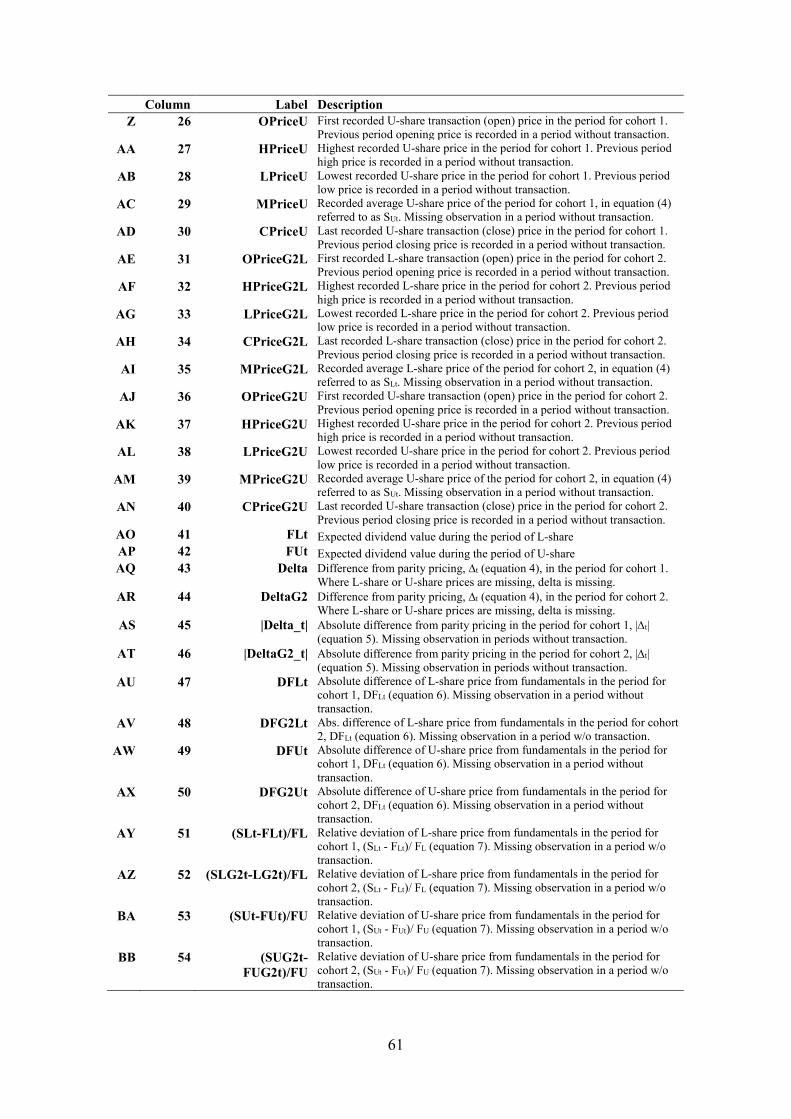
61
Column Label Description
Z 26 OPriceU First recorded U-share transaction (open) price in the period for cohort 1. Previous period opening price is recorded in a period without transaction.
AA 27 HPriceU Highest recorded U-share price in the period for cohort 1. Previous period high price is recorded in a period without transaction.
AB 28 LPriceU Lowest recorded U-share price in the period for cohort 1. Previous period low price is recorded in a period without transaction.
AC 29 MPriceU Recorded average U-share price of the period for cohort 1, in equation (4) referred to as SUt. Missing observation in a period without transaction.
AD 30 CPriceU Last recorded U-share transaction (close) price in the period for cohort 1. Previous period closing price is recorded in a period without transaction.
AE 31 OPriceG2L First recorded L-share transaction (open) price in the period for cohort 2. Previous period opening price is recorded in a period without transaction.
AF 32 HPriceG2L Highest recorded L-share price in the period for cohort 2. Previous period high price is recorded in a period without transaction.
AG 33 LPriceG2L Lowest recorded L-share price in the period for cohort 2. Previous period low price is recorded in a period without transaction.
AH 34 CPriceG2L Last recorded L-share transaction (close) price in the period for cohort 2. Previous period closing price is recorded in a period without transaction.
AI 35 MPriceG2L Recorded average L-share price of the period for cohort 2, in equation (4) referred to as SLt. Missing observation in a period without transaction.
AJ 36 OPriceG2U First recorded U-share transaction (open) price in the period for cohort 2. Previous period opening price is recorded in a period without transaction.
AK 37 HPriceG2U Highest recorded U-share price in the period for cohort 2. Previous period high price is recorded in a period without transaction.
AL 38 LPriceG2U Lowest recorded U-share price in the period for cohort 2. Previous period low price is recorded in a period without transaction.
AM 39 MPriceG2U Recorded average U-share price of the period for cohort 2, in equation (4) referred to as SUt. Missing observation in a period without transaction.
AN 40 CPriceG2U Last recorded U-share transaction (close) price in the period for cohort 2. Previous period closing price is recorded in a period without transaction.
AO 41 FLt Expected dividend value during the period of L-share
AP 42 FUt Expected dividend value during the period of U-share
AQ 43 Delta Difference from parity pricing, ∆t (equation 4), in the period for cohort 1. Where L-share or U-share prices are missing, delta is missing.
AR 44 DeltaG2 Difference from parity pricing, ∆t (equation 4), in the period for cohort 2. Where L-share or U-share prices are missing, delta is missing.
AS 45 |Delta_t| Absolute difference from parity pricing in the period for cohort 1, |∆t| (equation 5). Missing observation in periods without transaction.
AT 46 |DeltaG2_t| Absolute difference from parity pricing in the period for cohort 2, |∆t| (equation 5). Missing observation in periods without transaction.
AU 47 DFLt Absolute difference of L-share price from fundamentals in the period for cohort 1, DFLt (equation 6). Missing observation in a period without transaction.
AV 48 DFG2Lt Abs. difference of L-share price from fundamentals in the period for cohort 2, DFLt (equation 6). Missing observation in a period w/o transaction.
AW 49 DFUt Absolute difference of U-share price from fundamentals in the period for cohort 1, DFLt (equation 6). Missing observation in a period without transaction.
AX 50 DFG2Ut Absolute difference of U-share price from fundamentals in the period for cohort 2, DFLt (equation 6). Missing observation in a period without transaction.
AY 51 (SLt-FLt)/FL Relative deviation of L-share price from fundamentals in the period for cohort 1, (SLt - FLt)/ FL (equation 7). Missing observation in a period w/o transaction.
AZ 52 (SLG2t-LG2t)/FL Relative deviation of L-share price from fundamentals in the period for cohort 2, (SLt - FLt)/ FL (equation 7). Missing observation in a period w/o transaction.
BA 53 (SUt-FUt)/FU Relative deviation of U-share price from fundamentals in the period for cohort 1, (SUt - FUt)/ FU (equation 7). Missing observation in a period w/o transaction.
BB 54 (SUG2t-
FUG2t)/FU
Relative deviation of U-share price from fundamentals in the period for cohort 2, (SUt - FUt)/ FU (equation 7). Missing observation in a period w/o transaction.

62
B2.2 Data File (2): End of Period Subject DATA.xls
This file provides the data of the perfect correlation treatment and the no-correlation treatment. This file reveals the subject's purchases and sales during a period, the final share and cash holdings. Negative values indicate short positions. In total there were 174 subjects participating in 20 independent cohorts, 2 cohorts in 10 sessions, 4 sessions of the no-correlation treatment (see section B2.1 for more details). The following table describes the columns of data file (2) in more detail. Table B2.2 Detailed description - Data File (2): End of Period Subject DATA.xls
Column Label Description
A 1 Session Indicates the session by the date of initiation.
B 2 Correlation 1 indicates perfect correlation, 0 no correlation treatment
C 3 Cohort Sessions 1..6 for the perfect correlation, 7...10 no-correlation treatment; each session involved Group 1 and 2 as two independent cohorts
D 4 Market Indicates market 1..4 for the four markets of 10 periods
E 5 Period Indicates period 1..10 for the 10 periods per sequence
F 6 Subject Indicates participant's computer terminal 1..18 in the session
G 7 Cash Record of the subject's cash balance after dividend payment at the end of the period. Negative cash holdings indicate debt.
H 8 StockL Record of the subject's L-share units held at the end of the period. Negative numbers indicate a short position.
I 9 StockU Record of the subject's U-share units held at the end of the period. Negative numbers indicate a short position.
J 10 NumBuysL Number of L-shares the subject purchased in the period.
K 11 NumSellsL Number of L-shares the subject sold in the period.
L 12 NumBuysU Number of U-shares the subject purchased in the period.
M 13 NumSellsU Number of U-shares the subject sold in the period.
N 14 dZit Indicates the largest potential dividend in a period. For the single-period treatment, only the potential L-share dividend is indicated.
O 15 ProfitTrader Record of the subject's final cash balance, i.e., gains from trading shares and collecting dividends in the 10 periods of the market. Losses are cut at -500 CU.
P 16 ProfitObserver Record of the subject's final earnings from forecasting prices in the 10 periods of the market. Maximum gains are 600, deviations are punished; minimum is 0.
Q 17 ProfitTraderObserver Total earnings from market participation during a market sequence; sum of ProfitTrader and ProfitObserver. One market was chosen for payment by the roll of a die. Subjects were rewarded with an envelope containing this amount plus show-up fee and gains from warming-up-quizzes like CRT.

63
B2.3 Data File (3): Double Auction Trading DATA.xls This file provides the trading data for the perfect correlation treatment and the no-correlation treatment (including for tables 3C and 6). There were 20 independent cohorts as described in B2.1, 2 cohorts in 10 sessions. Subjects submitted limit orders for one unit; an ask indicates a proposed selling price, a bid indicates a proposed buying price. Transactions completed when one subject hit the immediate-buy button or the immediate-sell button confirming the best outstanding ask or bid. Only one share of asset could be transacted at a time. Each line in this data file corresponds to a limit order submitted for one share of asset. When a transaction completed, all outstanding bids of the buyer and all outstanding asks of the seller were cancelled (for both share classes). The transaction partners sellerID and BuyerID were recorded. Cancelled limit orders are indicated in the data file by a -2, and outstanding orders at the end of the period by -1. Trading was recorded in two independent tables, one for the L-share and one for the U-share. The order-book including the best outstanding bids and asks were not recorded, but were computed afterwards by the authors taking account of the chronological order of limit orders in the two tables and the recorded submission and transaction times. The following table describes the columns of data file (3) in more detail.
Table B2.3 Detailed description - Data File (3): Double Auction Trading DATA.xls
Column Label Description
A 1 Session Indicates the session by the date of initiation.
B 2 Session number Sessions 1..6 for the perfect correlation, 7...10 no-correlation treatment; each session involved two independent cohorts
C 3 Market Indicates market 1..4 for the four markets of 10 periods
D 4 Cohort Indicates the independent cohort that interacted in four markets of 10 periods. Cohorts 1..12 are data of the perfect correlation, 13..20 of the no-correlation treatment.
E 5 Period Indicates period 1..10 for the 10 periods per sequence
F 6 L 1 indicates submission in L-share market, 0 indicates U-share market
G 7 FV Dividend value of share in market in the submission period
H 8 SellerID Subject ID 1...18 of the seller / submitter of an offer to sell the share. If negative, there is no seller; -1 indicates the limit order remains open until the end; -2 indicates the limit order is closed automatically amid a purchase / transaction of the limit order submitter.
I 9 BuyerID Subject ID 1...18 of the buyer / submitter of a bid to purchase the share. If negative, there is no buyer; -1 indicates the limit order remains open until the end; -2 indicates the limit order is closed automatically amid a sale / transaction of the limit order submitter.
J 10 MakerID Subject ID 1...18 of the submitter of the limit order
K 11 Bid Recorded bidding (limit) price - price in cash units offered to buy the share
L 12 Ask Recorded asking (limit) price - price in cash units requested to sell the share
M 13 #ask Number of asks outstanding in same cohort / market / share at the time of asking order submission
N 14 #bid Number of asks outstanding in same cohort / market / share at the time of bidding order submission
O 15 LOL_ID L-Share limit order identifier assigned in chronological order; 1 indicates first limit order, 2 indicates the second, ... the highest number indicates the total number of limit orders recorded in the period for the L-share (for both cohorts)
P 16 LOU_ID U-Share limit order identifier assigned in chronological order; 1 indicates first limit order, 2 indicates the second, ... the highest number indicates the total number of limit orders recorded in the period for the U-share (for both cohorts)
Q 17 TPrice Recorded transaction price; if the limit order is accepted via immediate buy/sell, the transaction is recorded at the bidding or asking price of the limit order.

64
Column Label Description
R 18 TL_ID L-share transaction contract identifier assigned in chronological order; 1 indicates the first transaction, 2 the second one, ... the highest number indicates the number of L-share transactions in the period (for both cohorts). Missing observation w/o transaction.
S 19 TU_ID U-share transaction contract identifier assigned in chronological order; 1 indicates the first transaction, 2 the second one, ... the highest number indicates the number of U-share transactions in the period (for both cohorts). Missing observation w/o transaction.
T 20 SubmTime Recorded time of limit order submission in (remaining) seconds before market close.
U 21 TTime Recorded time of transaction in (remaining) seconds before market close.
V 22 CTime Computed time of closing the outstanding limit order.
W 23 BBidL Computed best L-share bid outstanding in cohort at time of limit order submission.
X 24 BAskL Computed best L-share ask outstanding in cohort at time of limit order submission.
Y 25 BBidU Computed best U-share bid outstanding in cohort at time of limit order submission.
Z 26 BAskU Computed best U-share ask outstanding in cohort at time of limit order submission.
AA 27 SameAsset
ArbitrageOpp
Computed dummy that takes value 1 if an arbitrage opportunities within the same asset exist, that is, when the best bid exceeds the best ask; 0 otherwise.
AB 28 DiscLMU Computed size of cross asset discrepancy, L minus U; exploitable (expected) gain by going long the L-share at the best ask and short the U-share at the best bid
AC 29 DiscUML Computed size of cross asset discrepancy, U minus L; exploitable (expected) gain by going long the U-share at the best ask and short the L-share at the best bid
AD 30 DiscDummy Computed dummy of outstanding discrepant limit order that takes value 1 if DLO exists, 0 otherwise
AE 31 DiscInitiation Computed dummy of discrepant limit order initiation (relevant for measure of equation 8) that takes value 1 if DLO is initiated, 0 otherwise
AF 32 DiscSizeInit Size of discrepant limit order at initiation; DiscLMU or DiscUML at initiation
AG 33 DiscMaker Computed subject ID of DLO submitter (relevant for measure of equation 8)
AH 33 TakerID Computed subject ID of DLO (relevant for measure of equation 8)
AI 33 HighExpReturnShare
ClosesFirstDummy
Computed dummy that takes value 1 if the high expected return trade closes first when a discrepant limit order is initiated (hypothesis 5A); 0 otherwise.

65
B2.4 Data File (4): Subject Characteristics DATA.xls This file provides the data of the subject characteristics by subject and averages by cohort for the perfect correlation treatment and the no-correlation treatment (including for tables 5A/B). There were 20 independent cohorts, 2 cohorts in 10 sessions, 6 sessions of the perfect correlation treatment (140520_1450, 140521_0936, 140521_1418, 140522_0905, 140530_0948, 140530_1600; names indicate initiation time (see B2.1)) and 4 sessions of the no-correlation treatment (140527_0951, 140529_0952, 140606_1501, 140609_1431). The following table describes the columns of data file (4) in more detail.
Table B2.4 Detailed description - Data File (4): Subject Characteristics DATA.xls
Column Label Description Recorded characteristics of each subject
A 1 Session Indicates the session by the date of initiation.
B 2 Cohort There were two independent cohorts per session. Cohorts 1..12 participated in the perfect correlation, cohorts 13...20 in the no-correlation treatment
C 3 Subject ID of the participant in a session. Each session was designed for 18 subjects (9 per cohort). Three cohorts had 7 subjects.
D 4 AvgPayoff Average trading gains of the subject in the four market sequences
E 5 CRT-score Measure of acuity which indicates the subject's number of correct answers {0, 1, 2, 3} in the Cognitive Reflection Task.
F 6 FEMALE Is the self-reported gender dummy; it takes 1 for female, 0 for male subjects
G 7 RiskAversion Measure of risk aversion elicited through the investment game task; it is the number {0, 1, ... , 100} of tokens the subject invested in the safe asset.
H 8 AGE Self-reported measure of participant's age on the day of the experiment.
I 9 THEO Self-reported measure of religiousness {0 secularist, 1 moderately religious, 2 devout religious}.
J 10 DLO Indicates the number of discrepant limit orders submitted by the subject
K 11 RFDLO_i Measure (equation 8) subject's rel frequency of DLO submission
L 12 APTITUDE Measure (1-RFDLO_i)
M 13 Nationality Indicates the self-reported origin of the subject
N 14 Studies Indicates the self-reported department/field of studies
Average characteristics of each cohort
O 15 sessionID Indicates the session by the date of the session.
P 16 cohortID The data involve 20 independent cohorts. Cohorts 1..12 participated in the perfect correlation treatment, cohorts 13...20 in the no-correlation treatment
Q 17 treatmentID Identifies treatment; 0 no-correlation, 1 perfect correlation treatment
R 18 CRT-share Average CRT-score in cohort
S 19 CRTxTreatDummy CRT-share x treatmentID
T 20 FemShare Average share of females in cohort
U 21 AvgRiskAversion Average measure of risk aversion (number of tokens in safe asset) in cohort
V 22 AvgAGE Average reported age in cohort
W 23 DiffParity Measure (equation 4) - deviation from parity pricing
X 24 DF Measure (equation 6) - relative absolute deviation from fundamentals
Y 25 PD Measure (equation 5) - cross-asset price discrepancy
Z 26 SumLO Total limit orders submitted in cohort
AA 27 SumDLO Total discrepant limit orders submitted in cohort
AB 28 RFDLO Measure (equation 8) relative frequency of discrepant limit order submission
AC 29 RD_L-Share Measure (equation 7) relative deviation for L-share
AD 30 RD_U-share Measure (equation 7) relative deviation for U-share
AE 31 RD_U-RD_L RD difference between U-share and L-share

66
B2.5 Data File (5): Additional treatments EOP Market DATA.xls
This file provides the data of the single-asset and the single-period treatments. In total there were 12 sessions; 161114_1454, 161115_0934, 161115_1507, 161116_1011, 161116_1658, 161117_0900, 161117_1435, 161118_0900, 170117_1457, 170118_ 0802, 170118_1443, 170119_1055. The session id indicates DayMonthYear_TimeOfInitiation, e.g., 161114_1454 indicates data collected in the session that was initiated at 2.54 pm on the 14th of November, 2016. In sessions (2), (3), (7), (8) there was a software bug (the dividend on the U-share was the maximum possible dividend always), resulting in invalid data. Data file (5) contains the valid data only. Server problems occurred in sessions 161114_1454 (implying a loss of data for the single asset treatment in period 10 of the second sequence), 170118_1443 (requiring a restart of the single period treatment after five periods), 170119_1055 (requiring a restart of the single period treatment after six periods). The following table describes the columns of data file (5) in more detail.
Table B2.5 Detailed description - Data File (5): Additional treatments EOP DATA.xls
Column Label Description
A 1 Session Indicates the session by the date of the session.
B 2 Run ID 1..3 for three market sequences of 10 periods, including one sequence of the single-period market, two sequences of the single-asset market
C 3 Period ID 1..10 for the 10 periods per sequence
D 4 NumPeriods Number of periods in the sequence
E 5 Correlation 1 indicates perfect correlation, 0 no correlation treatment
F 6 SinglePeriodTreatment 1 indicates single period, 0 single asset treatment
G 7 SingleAssetTreatment 1 indicates L-share, 2 U-share treatment, 0 single period treatment
H 8 InitialCash Cash endowment was 1200 units per period in single period, per sequence in single asset treatment, where it was carried over between periods.
I 9 InitialStockL Endowment of L-shares per period in single period, per sequence in single asset treatment, where shares were carried over between periods.
J 10 InitialStockU Endowment of U-shares per period in single period, per sequence in single asset treatment, where shares were carried over between periods.
K 11 numContracts Indicates the total number of submitted limit orders in both cohorts
L 12 numTradesG2L Indicates the number of L-share transactions in cohort 2
M 13 numTradesG2U Indicates the number of U-share transactions in cohort 2
N 14 numTradesL Indicates the number of L-share transactions in cohort 1
O 15 numTradesU Indicates the number of U-share transactions in cohort 1
P 16 DIV[1] Indicates the smallest potential dividend in a period. For the single-period treatment, only the potential L-share dividend is indicated.
Q 17 DIV[2] Indicates the second smallest potential dividend in a period. For the single-period treatment, only the potential L-share dividend is indicated.
R 18 DIV[3] Indicates the second largest potential dividend in a period. For the single-period treatment, only the potential L-share dividend is indicated.
S 19 DIV[4] Indicates the largest potential dividend in a period. For the single-period treatment, only the potential L-share dividend is indicated.
T 20 DividendL The recorded L-share dividend of the period
U 21 DividendU The recorded U-share dividend of the period
V 22 TimeAuction The time-length of market opening in seconds
W 23 OPriceL First recorded L-share transaction (open) price in the period for cohort 1
X 24 HPriceL Highest recorded L-share price in the period for cohort 1
Y 25 LPriceL Lowest recorded L-share price in the period for cohort 1

67
Column Label Description
Z 26 MPriceL Recorded average L-share price of the period for cohort 1, in equation (4) referred to as SLt. Missing observation in a period without transaction.
AA 27 CPriceL Last recorded L-share transaction (close) price in the period for cohort 1
AB 28 OPriceU First recorded U-share transaction (open) price in the period for cohort 1
AC 29 HPriceU Highest recorded U-share price in the period for cohort 1
AD 30 LPriceU Lowest recorded U-share price in the period for cohort 1
AE 31 MPriceU Recorded average U-share price of the period for cohort 1, in equation (4) referred to as SUt. Missing observation in a period without transaction.
AF 32 CPriceU Last recorded U-share transaction (close) price in the period for cohort 1
AG 33 OPriceG2L First recorded L-share transaction (open) price in the period for cohort 2
AH 34 HPriceG2L Highest recorded L-share price in the period for cohort 2
AI 35 LPriceG2L Lowest recorded L-share price in the period for cohort 2
AJ 36 CPriceG2L Last recorded L-share transaction (close) price in the period for cohort 2
AK 37 MPriceG2L Recorded average L-share price of the period for cohort 2, in equation (4) referred to as SLt. Missing observation in a period without transaction.
AL 38 OPriceG2U First recorded U-share transaction (open) price in the period for cohort 2
AM 39 HPriceG2U Highest recorded U-share price in the period for cohort 2
AN 40 LPriceG2U Lowest recorded U-share price in the period for cohort 2
AO 41 MPriceG2U Recorded average U-share price of the period for cohort 2, in equation (4) referred to as SUt
AP 42 CPriceG2U Last recorded U-share transaction (close) price in the period for cohort 2
AQ 43 FLt Expected dividend value during the period of L-share
AR 44 FUt Expected dividend value during the period of U-share
AS 45 Delta Difference from parity pricing (equation 4) in cohort 1
AT 46 DeltaG2 Difference from parity pricing (equation 4) in cohort 2
AU 47 (SLt-FLt)/FL Relative deviation of L-share price from fundamentals in the period for cohort 1, (SLt - FLt)/ FL (equation 7). Missing observation in a period w/o transaction.
AV 48 (SLG2t-LG2t)/FL Relative deviation of L-share price from fundamentals in the period for cohort 2, (SLt - FLt)/ FL (equation 7). Missing observation in a period w/o transaction.
AW 49 (SUt-FUt)/FU Relative deviation of U-share price from fundamentals in the period for cohort 1, (SUt - FUt)/ FU (equation 7). Missing observation in a period w/o transaction.
AX 50 (SUG2t-FUG2t)/FU Relative deviation of U-share price from fundamentals in the period for cohort 2, (SUt - FUt)/ FU (equation 7). Missing observation in a period w/o transaction.

68
Appendix C: Experimental Instructions (SEE JOURNAL OF
FINANCE WEBPAGE OR REQUEST FROM AUTHORS)
Experimental Instructions (main experiment)
• Perfect-correlation treatment
• No-correlation treatment
First part of the experiment (additional experiments)
• Perfect-correlation Single-period, first market round
• No-correlation Single-period, first market round
• Single-asset expected dividend 24, first 2 market rounds
• Single-asset expected dividend 48, first 2 market rounds
Further instructions (additional experiments)
• Further Instructions (perfect-correlation single-period)
• Further Instructions (no-correlation single-period)
• Further Instructions single-asset expected dividend 24, market
rounds 2, 3
Further Instructions single-asset expected dividend 48, market rounds 2, 3