Lower Bounds for Testing Graphical Models: Colorings and

Journal of Machine Learning Research 21 (2020) 1-62 Submitted 7/19; Revised 1/20; Published 2/20

Lower Bounds for Testing Graphical Models: Colorings andAntiferromagnetic Ising Models

Ivona Bezakova [email protected] Institute of TechnologyRochester, NY, USA

Antonio Blanca [email protected] State UniversityUniversity Park, PA, USA

Zongchen Chen [email protected] Institute of TechnologyAtlanta, GA, USA

Daniel Stefankovic [email protected] of RochesterRochester, NY, USA

Eric Vigoda [email protected]

Georgia Institute of Technology

Atlanta, GA, USA

Editor: Gabor Lugosi

Abstract

We study the identity testing problem in the context of spin systems or undirected graphicalmodels, where it takes the following form: given the parameter specification of the model Mand a sampling oracle for the distribution µM∗ of an unknown model M∗, can we efficientlydetermine if the two models M and M∗ are the same? We consider identity testing forboth soft-constraint and hard-constraint systems. In particular, we prove hardness resultsin two prototypical cases, the Ising model and proper colorings, and explore whether identitytesting is any easier than structure learning.

For the ferromagnetic (attractive) Ising model, Daskalakis et al. (2018) presented apolynomial time algorithm for identity testing. We prove hardness results in the antiferro-magnetic (repulsive) setting in the same regime of parameters where structure learning isknown to require a super-polynomial number of samples. Specifically, for n-vertex graphsof maximum degree d, we prove that if |β|d = ω(log n) (where β is the inverse temperatureparameter), then there is no polynomial running time identity testing algorithm unlessRP = NP . In the hard-constraint setting, we present hardness results for identity test-ing for proper colorings. Our results are based on the presumed hardness of #BIS, theproblem of (approximately) counting independent sets in bipartite graphs.

Keywords: distribution testing, structure learning, graphical models, Ising model, col-orings

©2020 Ivona Bezakova, Antonio Blanca, Zongchen Chen, Daniel Stefankovic, Eric Vigoda.

License: CC-BY 4.0, see https://creativecommons.org/licenses/by/4.0/. Attribution requirements are providedat http://jmlr.org/papers/v21/19-580.html.

https://creativecommons.org/licenses/by/4.0/

http://jmlr.org/papers/v21/19-580.html

Bezakova et al.

1. Introduction

We study the identity testing problem in the context of spin systems. Spin systems, alsoknown as Markov random fields or undirected graphical models, are a general frameworkin statistical physics, theoretical computer science and machine learning for modeling in-teracting systems of simple elements. In this type of model, the identity testing problem,sometimes also called goodness-of-fit testing, takes the following form: given the parameterspecification of the model M and a sampling oracle for the distribution µM∗ of an unknownmodel M∗, can we efficiently determine if the two models M and M∗ are the same?

A spin system consists of a finite graph G = (V,E) and a set S of spins; a configurationσ ∈ SV assigns a spin value to each vertex v ∈ V . The probability of finding the system ina given configuration σ is given by the Gibbs (or Boltzmann) distribution

µG,H(σ) =e−H(σ)

Z,

where Z is the normalizing factor known as the partition function and the Hamiltonian Hcontains terms that depend on the spin values at each vertex (a “vertex potential”) and ateach pair of adjacent vertices (an “edge potential”).

When µG,H(σ) > 0 for every configuration σ ∈ SV (i.e., the Gibbs distribution has fullsupport), the spin system is known as a soft-constraint model ; otherwise, it is called a hard-constraint model. This is a fundamental distinction among spin systems, as it determinestheir application domains and the computational complexity of several inherent problems.We provide here hardness results for identity testing for both soft-constraint and hard-constraint models by considering two prototypical systems: the Ising model and propercolorings.

A naive approach to the identity testing problem is to learn first the unknown model(G∗,H∗) and then check whether (G,H) = (G∗,H∗). The problem of learning G∗ fromsamples is known as structure learning and has received tremendous attention (see, e.g.,Chow and Liu, 1968; Dasgupta, 1999; Lee et al., 2007; Anandkumar et al., 2012; Ravikumaret al., 2010; Bresler et al., 2013, 2014b; Bresler, 2015; Vuffray et al., 2016; Hamilton et al.,2017; Klivans and Meka, 2017). Once the graph G∗ is known, it is often a simpler task toestimate H∗ (Bresler, 2015); this is known as the parameter estimation problem. Hence,one may be inclined to conjecture that identity testing is in fact easier than structurelearning, and we investigate whether or not this is the case. The main takeaway from ourresults is evidence that identity testing is as hard as structure learning for antiferromagnetic(repulsive) systems, as we show that the settings where these two problems are hard inboth the Ising model and proper colorings coincide.

1.1. Lower Bounds for the Ising Model

The Ising model is the quintessential example of a soft-constraint system and is studied in avariety of fields, including phylogeny (Felsenstein, 2004; Daskalakis et al., 2011), computervision (Geman and Graffigne, 1986; Roth and Black, 2005), statistical mechanics (Georgii,2011; Friedli and Velenik, 2017) and deep learning, where it appears under the guise ofBoltzmann machines (Ackley et al., 1985; Salakhutdinov and Larochelle, 2010; Salakhut-dinov and Hinton, 2012). The Ising model on a graph G = (V,E) is parameterized by

2

Lower Bounds for Testing Graphical Models

the inverse temperature β which controls the strength of the nearest-neighbor interactions.Configurations of the model are the assignments of spins S = +,− to the vertices of G.The probability of a configuration σ ∈ SV is given by the Gibbs distribution:

µG,β(σ) =eβ·A(σ)

ZG,β, (1)

where A(σ) is the number of edges of G connecting vertices with the same spin and ZG,β =∑σ∈SV exp(β · A(σ)) is the partition function; the associated Hamiltonian is H(σ) = −β ·

A(σ).

In the ferromagnetic case (β > 0) neighboring vertices prefer to align to the same spin,whereas the opposite happens in the antiferromagnetic setting (β < 0). In more generalvariants of the model, one can allow different inverse temperatures βe for each edge e ∈ E,as well as a vertex potential or external magnetic field. However, in this work, our emphasiswill be on lower bounds for the identity testing problem, and hence we focus on the abovementioned simpler homogeneous setting (all βe = β) with no external field.

The identity testing problem in the context of the Ising model is the following: given agraph G = (V,E), a real number β and oracle access to independent random samples froman unknown Ising distribution µG∗,β∗ , can we determine if (G, β) = (G∗, β∗)? If the modelsare distinct but their associated Gibbs distributions µG,β and µG∗,β∗ are exponentially closeto each other (measured by some notion of statistical distance between distributions as afunction of |V |), an exponential (in |V |) number of samples may be required to determinethat (G, β) 6= (G∗, β∗). Hence, following a large body of work on identity testing (see,e.g., Batu et al., 2001; Diakonikolas et al., 2015; Diakonikolas and Kane, 2016; Valiant andValiant, 2017; Diakonikolas et al., 2018; Daskalakis et al., 2018; Canonne et al., 2018), westudy this problem in the property testing framework (Rubinfeld and Sudan, 1996; Goldreichet al., 1998). That is, we are guaranteed that either (G, β) = (G∗, β∗) or ‖µG,β−µG∗,β∗‖ > ε,for some standard distance ‖ · ‖ between distributions and ε > 0 fixed.

The most common distances for identity testing are total variation distance and Kullback-Leibler (KL) divergence, and it is known that a testing algorithm for the latter immediatelyprovides one for the former (Daskalakis et al., 2018). Therefore, since our focus is on lowerbounds, we work with total variation distance, which we denote by ‖ · ‖tv.

Identity testing for the Ising model is then formally defined as follows. For positiveintegers n and d let M(n, d) denote the family of all n-vertex graphs of maximum degreeat most d.

Given a graph G ∈M(n, d), β ∈ R and sample access to a distribution µG∗,β∗ foran unknown Ising model (G∗, β∗), where G∗ ∈ M(n, d) and β∗ ∈ R, distinguishwith probability at least 3/4 between the cases:

1. µG,β = µG∗,β∗ ;

2. ‖µG,β − µG∗,β∗‖tv >13 .

As usual in the property testing setting, the choice of 3/4 for the probability of success isarbitrary, and it can be replaced by any constant in the interval (1

2 , 1) at the expense of a

3

Bezakova et al.

constant factor in the running time of the algorithm. The choice of 1/3 for the accuracyparameter is also arbitrary: we shall see in our proofs that our lower bounds hold for anyconstant ε ∈ (0, 1), provided n is sufficiently large; see also Remark 16.

Identity testing for the Ising model was studied by Daskalakis, Dikkala and Kamath (2018)who provided a polynomial time algorithm for the ferromagnetic Ising model (the β > 0case). (We will discuss their results in more detail after further discussion.) In contrast,we present lower bounds for the antiferromagnetic Ising model (β < 0). Our lower boundswill be for the case when β∗ = β, which means that they hold even under the additionalpromise that the hidden parameter β∗ is equal to β. (For a discussion of the case β∗ 6= β,as well as for some related open problems, see Section 8.) We mention that the hardnessof identity testing for general spin systems was previously considered by Bogdanov, Mosseland Vadhan (2008), but in the harder setup where there are hidden variables (some of thespins are not observed).

The structure learning and parameter estimation problems, which, as discussed earlier,can be used to solve the identity testing problem, have been particularly well-studied inthe context of the Ising model. Bresler (2015) presented a structure learning algorithmfor the Ising model that can learn G∗ ∈ M(n, d) in time eexp(O(|β∗|d2)) × O(n2 log n) andsample complexity eexp(O(|β∗|d2)) × O(log n). The dependency on the parameters β∗ andd was improved by Vuffray et al. (2016), who provide an algorithm to learn both G∗ andβ∗ with running time eO(|β∗|d) × O(n4 log n) and sample complexity eO(|β∗|d) × O(log n).More recently, Klivans and Meka (2017) provided a nearly optimal algorithm that learnsG∗ and β∗ in time eO(|β∗|d)×O(n2 log n) using eO(|β∗|d)×O(log n) samples; for other recentrelated work on the structure learning and parameter estimation problems for the Isingmodel see (Hamilton et al., 2017; Vuffray et al., 2019; Wu et al., 2019).

Consequently, when |β∗|d = O(log n), or when β = β∗ and |β|d = O(log n), structurelearning algorithms provide an identity testing algorithm with polynomial (in n) runningtime and sample complexity. In contrast, when |β∗|d = ω(log n) (i.e., |β∗|d/ log n→∞), it isknown that the structure learning problem cannot be solved in polynomial time (Santhanamand Wainwright, 2012), and this approach to identity testing fails.

Our first result is that the identity testing problem for the antiferromagnetic Ising modelis computationally hard in the same range of parameters. Specifically, we show that when|β|d = ω(log n)—or equivalently when β = β∗ and |β∗|d = O(log n)—there is no polynomialrunning time identity testing algorithm for M(n, d) unless RP = NP ; RP is the class ofproblems that can be solved in polynomial time by a randomized algorithm.

Theorem 1 Suppose n, d are positive integers such that 3 ≤ d ≤ nθ for constant θ ∈ (0, 1).If RP 6= NP , then for all real β < 0 satisfying |β|d = ω(log n) and all n sufficiently large,there is no polynomial running time algorithm to solve the identity testing problem for theantiferromagnetic Ising model in M(n, d).

In contrast to the above result, Daskalakis, Dikkala and Kamath (2018) designed an iden-tity testing algorithm for the Ising model with polynomial running time and sample complex-ity that works for arbitrary values of β (positive, negative or even non-homogeneous). Thisappears to contradict our lower bound in Theorem 1. However, the model in (Daskalakiset al., 2018) assumes not only sampling access to the unknown distribution µG∗,β∗ , butalso that the covariances between the spins at every pair of vertices in the visible graph

4


G = (V,E) are given. More precisely, they assume that for every u, v ∈ V the quantityEµG,β [XuXv] is known, where Xu, Xv ∈ +1,−1 are the random variables correspondingto the spins at u and v, respectively.

This is a reasonable assumption when these quantities can be computed (or approxi-mated up to an additive error) efficiently. However, an immediate consequence of our resultsis that in the antiferromagnetic setting when |β|d = ω(log n) there is no FPRAS1 for esti-mating EµG,β [XuXv] unless RP = NP . In a related result, Goldberg and Jerrum (Goldbergand Jerrum, 2019) showed recently that there is no FPRAS for (multiplicatively) approx-imating the pairwise covariances for the antiferromagnetic Ising model unless RP = #P .Further evidence for the hardness of this problem comes from the fact that sampling ishard in the antiferromagnetic setting (Sly and Sun, 2012; Galanis et al., 2016b) and in theferromagnetic model in the presence of inconsistent magnetic fields (Goldberg and Jerrum,2007) (i.e., the vertex potential of distinct vertices may have different signs). In summary,the algorithmic results of (Daskalakis et al., 2018) are most interesting for the ferromagneticIsing model (with consistent fields), where there are known polynomial running time algo-rithms for estimating the pairwise covariances (see, e.g., Jerrum and Sinclair, 1993; Randalland Wilson, 1999; Guo and Jerrum, 2017; Collevecchio et al., 2016).

In Theorem 1 we assume that |β|d = ω(log n), but our main technical result (Theorem 4)is actually more general. We show that when |β|d ≥ c lnn, where c > 0 is a sufficiently largeconstant, if there is an identity testing algorithm with running time T = T (n) and samplecomplexity L = L(n) then there is also a randomized algorithm with running time O(T+Ln)for computing the maximum cut of any graph with N = nΘ(1) vertices. Theorem 1 thenfollows immediately from the fact that either T or L ought to be super-polynomial in n, asotherwise we obtain a randomized algorithm for the maximum cut problem with polynomialrunning time; this would imply that RP = NP .

Under a stronger (but also standard) computational theoretic assumption, namely thatthere is no randomized algorithm with sub-exponential running time for the 3-SAT problem,i.e., the (randomized) exponential time hypothesis or rETH (Impagliazzo and Paturi, 2001;Calabro et al., 2008), our main theorem also implies a general lower bound for identitytesting that holds for all β and d satisfying |β|d ≥ c lnn.

Theorem 2 Suppose n, d are positive integers such that 3 ≤ d ≤ nθ for constant θ ∈(0, 1). Then, there exist constants c = c(θ) > 0 and α = α(θ) ∈ (0, 1) such that when|β|d ≥ c lnn, rETH implies that the running time T (n) of any algorithm that solves theidentity testing problem for the antiferromagnetic Ising model in M(n, d) satisfies T (n) ≥min

exp(Ω(nα)), exp(Ω(|β|d))

n

.

We remark that the bound in this theorem is comparable to the exp(Ω(|β|d)) lowerbound for the sample complexity of structure learning (Santhanam and Wainwright, 2012),albeit requiring that rETH is true. We also mention that the lower bounds in Theorems 1and 2 are both much stronger than the Ω(

√n) lower bound in (Daskalakis et al., 2018).

1. A fully polynomial-time randomized approximation scheme (FPRAS) for an optimization problem withoptimal solution Z produces an approximate solution Z such that, with probability at least 1 − δ,(1− ε)Z ≤ Z ≤ (1 + ε)Z with running time polynomial in the instance size, ε−1 and log(δ−1).

5

Bezakova et al.

The very high level idea of the proof of our main theorem for the Ising model (Theo-rem 4), from which Theorems 1 and 2 are derived as corollaries, is as follows: given a graphH and an integer k, we construct an identity testing instance Λ so that the output of theidentity testing algorithm on Λ can be used to determine whether there is a cut in H of sizeat least k. A crucial component in our construction is a “degree reducing” gadget, whichconsists of a random bipartite graph and is inspired by similar random gadgets in seminalworks on the hardness of approximate counting (Sly, 2010). One of the main technical chal-lenges in the paper is to establish precise bounds on the edge expansion of these randomgadgets. A detailed overview of our proof is given in Section 2.1.

1.2. Lower Bounds for Proper q-colorings

The proper q-colorings of a graph G = (V,E) constitute a canonical hard-constraint spinsystem, with multiple applications in statistical physics and theoretical computer science.In this model, the vertices of graph G are assigned spins (or colors) from 1, . . . , q, andthe Gibbs distribution µG becomes the uniform distribution over the proper q-coloringsof the graph G. The identity testing problem for this model in M(n, d) is defined asfollows: given q, a graph G ∈ M(n, d) and sample access to random q-colorings of anunknown graph G∗ ∈M(n, d), distinguish with probability at least 3/4 whether µG = µG∗

or ‖µG − µG∗‖ > 1/3.

We establish lower bounds for this problem, thus initiating the study of identity testing inthe context of hard-constraint spin systems. While identity testing does not seem to havebeen studied in this context before, the related structure learning problem has receivedsome attention (Bresler et al., 2014a; Blanca et al., 2018). For proper colorings, it isknown that when q ≥ d+ 1 the hidden graph G can be learned from poly(n, d, q) samples,whereas when q ≤ d then the problem is non-identifiable, i.e., there are distinct graphswith the same collection of q-colorings (Blanca et al., 2018). Moreover, for d ≥ dc(q) =q +

⌈√q⌉− 1, or equivalently q ≤ d−

√d+ Θ(1), it was also established in (Blanca et al.,

2018) that the easier equivalent structure learning problem (learning any graph with thesame collection of q-colorings as the unknown graph) is computationally hard in the sensethat the sample complexity is exponential in n. The threshold dc(q) coincides exactly withthe one for polynomial time/NP-completeness for the problem of determining if G is q-colorable (Emden-Weinert et al., 1998; Molloy and Reed, 2001); see (22) for the precisedefinition of dc(q).

We prove here that the identity testing problem is also hard when d ≥ dc(q), thus estab-lishing another connection between the hardness of identity testing and structure learning.For this we utilize the complexity of #BIS, which is the problem of counting the inde-pendent sets in a bipartite graph. #BIS is believed not to have an FPRAS, and it hasachieved considerable interest in approximate counting as a tool for proving relative com-plexity hardness (see, e.g., Dyer et al., 2004; Goldberg and Jerrum, 2012; Dyer et al., 2010;Bulatov et al., 2013; Chen et al., 2015; Cai et al., 2016; Galanis et al., 2016a).

Theorem 3 Suppose n, d and q are positive integers such that q ≥ 3 and d ≥ dc(q). If#BIS does not admit an FPRAS, then there is no polynomial running time algorithm thatsolves the identity testing problem for proper q-colorings in M(n, d).

6


In the proof of this theorem we reduce the #BIS-hard problem of counting 3-coloringsin bipartite graphs to identity testing for q-colorings. The high level idea of our proof is asfollows: given a bipartite graph H and an approximation Z for the number of 3-coloringsZ3(H) of H, we construct an identity testing instance that depends on both H and thevalue of Z. We then show how to use an identity testing algorithm on this instance to checkwhether Z is an upper or lower bound for Z3(H). By adjusting Z and repeating this processwe converge to a good approximation for Z3(H). A crucial element in our construction isagain the design of a degree reducing gadget; in this case, our gadget is inspired by similarconstructions in (Emden-Weinert et al., 1998; Molloy and Reed, 2001; Blanca et al., 2018) forestablishing the computational hardness of the decision and (equivalent) structure learningproblems for d ≥ dc(q). Finally, we mention that for 3-colorings, dc(3) = 4 and thus ourhardness result holds for all graphs with maximum degree at least 4.

1.3. An Algorithm for the Ferromagnetic Ising Model

We provide an improved algorithm for the ferromagnetic Ising model. As mentioned, bycombining the algorithm in (Daskalakis et al., 2018) with previous results for sampling (seeJerrum and Sinclair, 1993; Randall and Wilson, 1999; Guo and Jerrum, 2017; Collevecchioet al., 2016), one obtains a polynomial running time algorithm for identity testing in theferromagnetic setting. The algorithm in (Daskalakis et al., 2018) works for symmetric-KLdivergence which is a stronger notion of distance. We show that if one considers insteadtotal variation distance, then there is a polynomial running time algorithm that solves theidentity testing problem with sample complexity O(n2d2ε−2). This is an improvement overthe O(n2d2β2ε−2) bound in (Daskalakis et al., 2018), as there is no dependence on theinverse temperature β. See Theorem 30 in Section 6 for a precise statement of this result.

The rest of the paper is organized as follows. In Section 2 we state our main technicaltheorem (Theorem 4), and we derive Theorems 1 and 2 as corollaries. In Section 2.1, wesketch the key ideas in the proof our main result. The actual proof of Theorem 4 is fleshedout in Section 4. Before that, we introduce a useful variant of the maximum cut problem andstudy its complexity in Section 3. In Section 5 we provide bounds for the edge expansion ofrandom bipartite graphs which are crucially used in our proofs and could be of independentinterest. Our algorithm for the ferromagnetic Ising model is analyzed in Section 6, and ourresults for proper q-colorings (Theorem 3) are derived in Section 7; specifically, the reductionfor the q ≥ 4 case is presented in Section 7.4, and the more elaborate construction for q = 3is given in Section 7.5.

2. Lower Bounds for the Ising Model

To establish our lower bounds in Theorems 1 and 2 we use the computational hardness ofthe maximum cut (MaxCut) problem. Recall that in the search variant of this problem,given a graph H and an integer k > 0, the goal is to determine whether there is a cut ofsize at least k in H. Our main technical result, from which Theorems 1 and 2 are derived,is the following.

Theorem 4 Suppose n and d are positive integers such 3 ≤ d ≤ n1−ρ for some constantρ ∈ (0, 1). Then, for all n sufficiently large, there exist c = c(ρ) > 0 and an integer

7

Bezakova et al.

N = Θ(nmin ρ4, 114) such that when |β|d ≥ c lnn, any identity testing algorithm for M(n, d)

for the antiferromagnetic Ising model with running time T (n) and sample complexity L(n) ≤exp(|β|d/c)

30n provides a randomized algorithm for MaxCut on any graph with N vertices. Thisalgorithm outputs the correct answer with probability at least 11/20 and has running timeO(T (n) + n · L(n)).

In words, this theorem says that under some mild assumptions, when |β|d ≥ c lnn, anyidentity testing algorithm with running time T (n) and sample complexity L(n) provides arandomized algorithm for MaxCut on graphs of poly(n) size with running time O(T (n) +n ·L(n)). The high level ideas in the proof of this theorem are described next in Section 2.1;its actual proof is fleshed out in Section 4. Several important consequences of this result,including Theorems 1 and 2 from the introduction, are derived in Section 2.2.

2.1. Main Result for the Ising Model: Proof Overview

To establish Theorem 4 we construct a class N of n-vertex graphs of maximum degree atmost d and show how an algorithm that solves identity testing for N ⊂ M(n, d) can beused to solve the MaxCut problem on graphs with N = Θ(nα) vertices, where α ∈ (0, 1) isa constant. (The exact value for α depends on d: if d = O(1), then we can take α = 1/14;otherwise, we set α = ρ/4.)

Suppose we want to solve the MaxCut problem for a graph H = (V,E) and k ∈ N.At a high level, we use H and k to construct an identity testing instance consisting of anantiferromagnetic Ising model M , which plays the role of the visible model, and samplesfrom a simpler model M∗. Our construction of these two models ensures that samplingfrom M∗ is easy, and that the output of the testing algorithm reveals information about themaximum cuts of H. To implement this approach, we consider a variant of the MaxCutproblem which we call the TwoLargeCuts problem. We shall see that this problem isalso NP-hard (by a reduction from MaxCut).

An instance of the TwoLargeCuts problem is constructed as follows. Given H =(V,E) and k ∈ N, we add two vertices s and t to H and connect both s and t to everyvertex in V with N = |V | edges (adding a total of 2N2 edges); we also add w edges betweens and t. Let Hw be the resulting multigraph. (In our proofs we will convert Hw into asimple graph, but it is conceptually simpler to consider the multigraph for now.) The cut(s, t, V ) in Hw is of size 2N2.

In the TwoLargeCuts problem the goal is to determine whether there are at leasttwo cuts in Hw of size at least 2N2 (see Definition 8). MaxCut can be reduced toTwoLargeCuts by treating w, the number of edges between s and t, as a parameter.Specifically, if (S, V \S) is a cut of size k in the original graph H, then (S∪s, (V \S)∪t)is a cut of size

w + k +N |S|+N |V \ S| = w + k +N2

in Hw. Hence, (s, t, V ) is the unique large cut (i.e., cut of size ≥ 2N2) if and only if

w + MaxCut(H) +N2 < 2N2,

where MaxCut(H) denotes the size of the maximum cut of H. Therefore, to solveMaxCut for H and k, it is sufficient to solve the TwoLargeCuts problem for Hw with

8


w = N2 − k; see Section 3 for the proof of this fact. This yields that the TwoLargeCutsproblem is NP-complete and the following useful lemma.

Lemma 5 Let H = (V,E) be an N -vertex graph and let δ ∈ (0, 1/2]. Suppose there existsa randomized algorithm that solves the TwoLargeCuts problem on inputs H and w ≤ N2

with probability at least 1/2 + δ and running time R. Then, there exists a randomizedalgorithm to solve MaxCut for H and k ∈ N with running time R + O(N2) and successprobability at least 1/2 + δ.

To solve the TwoLargeCuts problem, we can use the antiferromagnetic Ising modelon Hw to determine if (s, t, V ) is the maximum cut of Hw as follows. Every Ising config-uration of Hw determines a cut: all the “+” vertices belong to one side of the cut and the“−” vertices to the other (or vice versa). Observe that for every cut of Hw there are exactlytwo corresponding Ising configurations. The intuition is that the maximum cuts of Hw

correspond to the configurations of maximum likelihood in the Gibbs distribution. Indeed,when |β| is sufficiently large, the distribution will be well-concentrated on the configurationsthat correspond to the maximum cuts. Therefore, a sample from the Gibbs distributionwould reveal with high probability whether or not (s, t, V ) is the maximum cut of Hw

and thus solve the TwoLargeCuts problem.

To simulate large magnitudes of β, we strengthen the interactions between neighboringvertices of Hw by replacing every edge by 2` edges. However, sampling from the antifer-romagnetic Ising distribution on the resulting multigraph Hw,` is a hard problem, and wewould need to provide a sampling procedure. Instead, we use the identity testing algorithmas follows. We construct a simpler Ising model M∗ with two key properties: (i) we can easilygenerate samples from M∗ and (ii) M∗ is close in total variation distance to the Ising modelM = (Hw,`, β) if and only if (s, t, V ) is the unique large cut of Hw. Our construction of

M∗ is facilitated by our construction of the TwoLargeCuts instance Hw where there is atrivial (easy to find) large cut; i.e., the cut (s, t, V ). (The precise construction of M andM∗ is described in Section 4, and their desired properties are established in Sections 4.2and 4.3.) Then, we give Hw,`, the parameter β and samples from M∗ as input to the tester.If the tester outputs Yes, it means that it regarded the samples from M∗ as samples fromM and so (s, t, V ) must be the unique large cut of Hw. Conversely, if the tester outputsNo, then the total variation distance between µM and µM∗ must be large, in which case(s, t, V ) is not the unique large cut of Hw.

In summary, this argument implies that an identity testing algorithm for n-vertex multi-graphs gives a polynomial time randomized algorithm for MaxCut on graphs with n − 2vertices. However, the maximum degree of Hw,` depends on `, N and w and could bemuch larger than d. Hence, this argument does not apply for small values of d, even if weoverlook the fact that we would be using identity testers for multigraphs instead of graphs.To extend the argument to simple graphs in M(n, d) for all 3 ≤ d ≤ n1−ρ, we introducea “degree reducing” gadget, which is reminiscent of gadgets used in works concerning thehardness of approximate counting (Sly, 2010; Sly and Sun, 2012).

Every vertex of Hw,` is replaced by a random bipartite graph G = (L ∪ R,EG); seeSection 4 for the precise random graph model. The graph G has maximum degree at mostd, and some of its vertices, which we call ports, will have degree strictly less than d, so

9

Bezakova et al.

that they can be used for connecting the gadgets as indicated by the edges of Hw,`. The

resulting simple graph, which we denote by HΓw, will have maximum degree d. (Γ is the set

of parameters of our random graph model; see Section 4 for the details.) In similar manneras described above for Hw,`, an identity testing algorithm for the antiferromagnetic Ising

model on HΓw can be used to determine whether (s, t, V ) is the unique large cut of Hw;

see Lemma 12. Since HΓw has maximum degree at most d, Theorem 4 follows.

Finally, we mention that the main technical challenge in our approach is to establishthat in every gadget, with high probability, either every vertex of L is assigned “+” andevery vertex of R is assigned “−” or vice versa; see Theorems 10 and 11. To show this, werequire very precise bounds on the edge expansion of the random bipartite graph G. Whend → ∞, these bounds can be derived in a fairly straightforward manner from the resultsin (Brito et al., 2018). However, the case of d = O(1) is more difficult, and it requiresfor us to define the notion of edge expansion with respect to the ports of the gadget andextending some of the ideas in (Hoory et al., 2006) (see Theorem 19). Our bounds for theedge expansion of random bipartite graphs may be of independent interest; see Section 5.

2.2. Consequences of Main Result for the Ising Model: Proofs of Theorems 1and 2

In this section we show how to derive Theorems 1 and 2 from Theorem 4. For Theorem 1we also use the fact that there is no randomized algorithm for MaxCut with polynomialrunning time unless RP = NP . (We recall that RP is the class of problems that can besolved in polynomial time by a randomized algorithm.) For Theorem 2 we use a strongerassumption, namely the (randomized) exponential time hypothesis (or rETH) (Impagliazzoand Paturi, 2001; Calabro et al., 2008).

Proof of Theorem 1 Suppose there is an identity testing algorithm for M(n, d) withpoly(n) running time and sample complexity; that is, L ≤ T = poly(n). Since |β|d =ω(lnn),

L ≤ exp (|β|d/c)30n

.

Hence, Theorem 4 implies there is a randomized algorithm for MaxCut on graphs of sizeN = Θ(nmin ρ

4, 114) that succeeds with probability at least 11/20 and has running time

O(T + Ln) = poly(n). This implies that MaxCut is in BPP . (BPP is the class of alldecision problems solvable in polynomial time with success probability greater than 1/2 onboth “yes” and “no” instances; in contrast, RP only allows errors on “no” instances.) SinceMaxCut is NP -complete, then NP ⊆ BPP , and the result follows from the standard factthat if NP ⊆ BPP , then RP = NP ; see, e.g., (Ko, 1982).

Proof of Theorem 2 Suppose there exists an identity testing algorithm with runningtime T and sample complexity L. If L > exp(|β|d/c)

30n , then

T ≥ L > exp (|β|d/c)30n

and the result follows. Otherwise, when |β|d ≥ c lnn for a suitable constant c = c(ρ) > 0,Theorem 4 implies that there exists a randomized algorithm for MaxCut on graphs with

10


N = Θ(nmin ρ4, 114) vertices with running time at most O(T + Ln) and success probability

at least 11/20. However, under the assumption that rETH is true, there is no randomizedalgorithm for MaxCut in such graphs with running time eo(n

α), where α = minρ4 ,114.

Thus, there exist constants δ, γ > 0 such that

δ(T + Ln) ≥ eγnα.

Consequently, if L ≤ eγnα

2δn , then T ≥ eγnα

2δ ; otherwise T ≥ L ≥ eγnα

2δn . Putting these boundstogether we get

T ≥ min

exp(|β|d/c)

30n,exp(γnα)

2δn

,

and the result follows.

Finally, we note that Theorem 4 also implies a polynomial (in n) lower bound for therunning time of any identity testing algorithm when |β|d = Θ(log n). This regime is notcovered by Theorem 1, where the assumption is that |β|d = ω(log n), and Theorem 2 appliesto this setting, but under the stronger rETH assumption. Our next theorem shows thatthe weaker complexity theoretic assumption RP 6= NP suffices.

Theorem 6 Suppose n, d are positive integers such 3 ≤ d ≤ n1−ρ for some constantρ ∈ (0, 1) and β < 0 is such that |β|d > c lnn, where c = c(ρ) is the constant fromTheorem 4. If RP 6= NP , then, for all n sufficiently large, any algorithm that solves theidentity testing problem forM(n, d) for the antiferromagnetic Ising model has running time

T = Ω(n∆), where ∆ = |β|dc lnn − 1.

Proof Suppose there is an identity testing algorithm forM(n, d) with running time T and

sample complexity L. We consider two cases. First, if L ≤ exp(|β|d/c)30n , then Theorem 4 im-

plies that there is a randomized algorithm for MaxCut on graphs with N = Θ(nmin ρ4, 114)

vertices that has running time O(T + Ln) and success probability 11/20. Therefore,T + Ln = nω(1) since otherwise NP ⊆ BPP and thus RP = NP (Ko, 1982). Hence,if Ln = O(poly(n)), then T = Ω(nω(1)); otherwise T ≥ L = Ω(nω(1)). For the second case,

when L > exp(|β|d/c)30n , we have

T ≥ L > exp (|β|d/c)30n

=n∆

30,


3. Hardness of the TwoLargeCuts Problem

In this section we prove Lemma 5, where the hardness of the TwoLargeCuts problemis established. Recall that the TwoLargeCuts problem is a variant of the MaxCutproblem which we will reduce to the identity testing problem. We formally define theTwoLargeCuts problem next.

11

Bezakova et al.

Definition 7 Let H = (V,E) be a graph and let w ∈ N. Let Hw = (V , E) be the multigraphdefined as follows:

1. V contains all vertices in V and two new vertices s and t; i.e., V = V ∪ s, t;

2. E contains all edges in E, N copies of edges s, v and t, v for each v ∈ V , and wcopies of the edge s, t.

Observe that the cut (s, t, V ) contains exactly 2N2 edges.

Definition 8 In the TwoLargeCuts problem, given a graph H and w ∈ N, the goal is todetermine whether there are at least two cuts in Hw of size at least 2N2.

Lemma 5 is a direct corollary of the following lemma, which implies that MaxCut can bereduced to TwoLargeCuts.

Lemma 9 Let H = (V,E) be an N -vertex graph and let w ∈ N. The cut (s, t, V ) is theunique maximum cut of Hw if and only if MaxCut(H) < N2 − w.

Consequently, to solve MaxCut on inputsH and k, it is sufficient to solve the TwoLargeCutsproblem for Hw with w = N2−k. Hence, Lemma 5 is a direct corollary of Lemma 9. (Notethat Lemma 9 also implies that the TwoLargeCuts problem is NP-complete.)

Proof of Lemma 9 Let (S, T ) be a cut of Hw (i.e., S ∪ T = V and S ∩ T = ∅) and letEHw(S, T ) ⊆ E be the set of edges between S and T in Hw. Similarly, for S′, T ′ ⊆ V , letEH(S′, T ′) ⊆ E be the set of edges between S′ and T ′ in H.

Let us consider first the cuts (S, T ) where s and t belong to the same set. Without lossof generality assume s, t ∈ S, and let S0 = S \ s, t. Then, (S0, T ) is a cut of H and so∣∣∣EHw(S, T )

∣∣∣ =∣∣∣EHw(S0, T )

∣∣∣+∣∣∣EHw(s, t, T )

∣∣∣ = |EH(S0, T )|+ 2N |T | ≤ (N − |T |)|T |+ 2N |T |.

The quadratic function f(x) = (N − x)x + 2Nx is maximized at x = N for 0 ≤ x ≤ N

and f(N) = 2N2. Thus,∣∣∣EHw(S, T )

∣∣∣ ≤ 2N2, and the maximum value 2N2 can be attained

only when |T | = N ; i.e., S0 = ∅ and (S, T ) = (s, t, V ).Now, for the cuts where s and t belong to distinct sets of the cut, let us assume without

loss of generality that s ∈ S and t ∈ T . Let S0 = S\s and T0 = T \ t. Then, (S0, T0) isa cut of H, and∣∣∣EHw(S, T )

∣∣∣ =∣∣∣EHw(S0, T0)

∣∣∣+∣∣∣EHw(S0, t)

∣∣∣+∣∣∣EHw(s, T0)

∣∣∣+∣∣∣EHw(s, t)

∣∣∣= |EH(S0, T0)|+N2 + w.

Hence, the maximum cut of this class corresponds to the case when (S0, T0) is a maximumcut of H, and ∣∣∣EHw(S, T )

∣∣∣ = MaxCut(H) +N2 + w.

Combining the above two cases, we conclude that (s, t, V ) is the unique maximum cutof Hw if and only if 2N2 > MaxCut(H) +N2 + w, and the result follows.

12


4. Proof of Main Result for the Ising Model: Theorem 4

We describe our gadget for the Ising model first. Suppose m, p, d, din, dout ∈ N+ are positiveintegers such that m ≥ p, d ≥ 3 and din + dout = d. Let G = (VG, EG) be the randombipartite graph defined as follows:

1. Set VG = L ∪R, where |L| = |R| = m and L ∩R = ∅;

2. Let P be subset of VG chosen uniformly at random among all the subsets such that|P ∩ L| = |P ∩R| = p;

3. Let M1, . . . ,Mdin be din random perfect matchings between L and R;

4. Let M ′1, . . . ,M′dout

be dout random perfect matchings between L\P and R\P ;

5. Set EG =(⋃din

i=1Mi

)∪(⋃dout

i=1 M′i

);

6. Make the graph G simple by replacing multiple edges with single edges.

We use G(m, p, din, dout) to denote the resulting distribution; that is, G ∼ G(m, p, din, dout).Vertices in P are called ports. Every port has degree at most din while every non-port vertexhas degree at most d.

In our proofs, we use instances of this random graph model with two different choicesof parameters. For the case when d is such that 3 ≤ d = O(1), we choose p =

⌊m1/4

⌋,

din = d− 1 and dout = 1; otherwise we take p = m (i.e., every vertex is a port), din = bθdcand dout = d − bθdc for a suitable constant θ ∈ (0, 1). For both parameter choices weestablish that the random graph G is a good expander with high probability; see Section 5.Using this, we can show that there are only two “typical” configurations for the Ising modelon G, even in the presence of an external configuration (i.e., a boundary condition) exertinginfluence on the configuration of G via its ports.

We present some notation next that will allow us to formally state these facts. Letσ+(G) be the configuration of G = (L∪R,EG) where every vertex in L is assigned “+” andevery vertex in R is assigned “−”; similarly, define σ−(G) by interchanging “+” and “−”.To capture the notion of an external configuration for the bipartite graph G, we assume thatG is an induced subgraph of a larger graph G′ = (VG′ , EG′). Let ∂P = VG′ \ VG. Assumethat every vertex in P ⊆ VG is connected to up to dout vertices in ∂P and that there are noedges between VG \P and ∂P in G′. We use ∂P = τ for the event that the configurationin G′ of ∂P is τ ∈ +,−∂P . We can show that for any τ , with high probability over thechoice of the random graph G, the Ising configuration of VG on G′ conditioned on ∂P = τwill likely be σ+(G) or σ−(G).

Theorem 10 Suppose β < 0, 3 ≤ d = O(1), din = d − 1, dout = 1 and p = bmαc, whereα ∈ (0, 1

4 ] is a constant independent of m. Then, there exists a constant δ > 0 such thatwith probability 1−o(1) over the choice of the random graph G the following holds for everyconfiguration τ on ∂P :

µG′,β(σ+(G), σ−(G) | ∂P = τ) ≥ 1− 2m

eδ|β|d.

13

Bezakova et al.

Theorem 11 Suppose β < 0, p = m and 4 + 1200ρ ≤ d ≤ m

1−ρ for some constant ρ ∈ (0, 1)independent of m. Then, there exist constants δ = δ(ρ) > 0 and θ = θ(ρ) ∈ (0, 1) such thatwhen din = bθdc and dout = d − bθdc the following holds for every configuration τ on ∂Pwith probability 1− o(1) over the choice of the random graph G:

µG′,β(σ+(G), σ−(G) | ∂P = τ) ≥ 1− 2m

eδ|β|d.

The proofs of these theorems are given in Section 5.

4.1. Testing Instance Construction

Let H = (V,E) be a simple N -vertex graph and for w ≤ N2 let Hw be the multigraphfrom Definition 7. We use an instance of the random bipartite graph G(m, p, din, dout) as agadget to define a simple graph HΓ

w, where Γ denotes the set parameters m, p, din, dout, `;` > 0 is assumed to be an integer divisible by dout. The graph HΓ

w is constructed as follows:

1. Generate an instance G = (L ∪R,EG) of the random graph model G(m, p, din, dout);

2. Replace every vertex of Hw by a copy Gv = (Lv ∪Rv, EGv) of the generated instanceG;

3. For every edge v, u ∈ Hw, choose `/dout unused ports in Lv and `/dout unusedports in Lu and connect them with a simple bipartite dout-regular graph;

4. Similarly, for every edge v, u ∈ Hw, choose `/dout unused ports in Rv and `/dout

unused ports in Ru and connect them with a simple bipartite dout-regular graph.

Observe that our construction requires:

din + dout = d ≤ m, (2)

dout | `, (3)

`(N2 + w) ≤ p · dout, (4)

d2out ≤ `. (5)

To see that (4) is necessary, note that the maximum degree of Hw is N2 + w (this is thedegree of vertices s and t), and so the total out-degree of the ports should be large enoughto accommodate `(N2 + w) edges. Observe also that when condition (5) holds, there isalways a simple bipartite dout-regular graph with `/dout vertices on each side for steps 3and 4.

The number of vertices in HΓw is 2m(N + 2) and its maximum degree is d = din + dout;

thus, HΓw ∈M(2m(N+2), d). Let I be an independent set with N vertices. By setting H =

I and w = 0, we can analogously define the graphs I0 and IΓ0 so that IΓ

0 ∈M(2m(N+2), d).Let M and M∗ denote the Ising models (HΓ

w, β) and (IΓ0 , β), respectively. Our testing

instance will consist of the model M and (approximate) samples from M∗. We show nextthat the models M and M∗ are statistically close if and only if (s, t, V ) is the unique largecut of Hw.

14


4.2. Relating the Ising Models M and M∗

To formally study the relationship between the models M and M∗ we require some addi-tional notation. For a configuration σ on HΓ

w, we say that the gadget Gv=(Lv ∪Rv, EGv) isin the plus (resp., minus) phase if all the vertices in Lv (resp., Rv) are assigned “+” in σ andall the vertices in Rv (resp., Lv) are assigned “−”. Let Ωgood be the set of configurations

of HΓw where the gadget of every vertex is either in the plus or the minus phase. The set

of Ising configurations of HΓw and IΓ

0 is the same and is denoted by Ω. We use ZM , ZM∗

for the partition functions of M , M∗, and ZM (Λ), ZM∗(Λ) for their restrictions to a subsetof configurations Λ ⊆ Ω. That is, ZM =

∑σ∈ΩwM (σ) and ZM (Λ) =

∑σ∈ΛwM (σ) where

wM (σ) := eβA(σ) is called the weight of the configuration σ in M ; see (1). When β < 0,wM (σ) = e−|β|A(σ).

The Ising models M and M∗ are related as follows.

Lemma 12 Let N ≥ 1, w ≥ 0 be integers and let β < 0. Let Γ = (m, p, din, dout, `) be suchthat |β|(`−d) ≥ N and conditions (2)—(5) are satisfied. If for the Ising model M = (HΓ

w, β)we have ZM (Ωgood) ≥ (1− ε)ZM for some ε ∈ (0, 1), then with probability 1− o(1) over thechoice of the random graph G the following holds:

1. If (s, t, V ) is the unique maximum cut of Hw, then

‖µM − µM∗‖tv ≤ 2(ε+ e−2|β|d).

2. If (s, t, V ) is not the unique maximum cut of Hw, then

‖µM − µM∗‖tv >1

2− ε− e−2|β|d.

3. If there is a cut in Hw with strictly more edges than (s, t, V ), then

‖µM − µM∗‖tv ≥ 1− ε− 2e−2|β|d.

Let σ+ = σ+(HΓw) be the configuration of HΓ

w such that the gadgets for s and t are inthe plus phase and every other gadget is in the minus phase; define σ− = σ−(HΓ

w) in similarmanner but interchanging “+” and “−” everywhere. Let Ω0 = Ω0(HΓ

w) = σ+, σ−. Wewill use the following fact to prove Lemma 12.

Fact 13 Let N ≥ 1 be an integer and let β < 0. Let Γ = (m, p, din, dout, `) be such that|β|(`N − d) ≥ N and conditions (2)—(5) are satisfied. If for the Ising model M∗ = (IΓ

0 , β)we have ZM∗(Ωgood) ≥ (1− ε)ZM∗ for some ε ∈ (0, 1), then µM∗(Ω

0) ≥ 1− ε− e−2|β|d.

Proof The weight of the configurations σ+, σ− satisfy: wM∗(σ+) = wM∗(σ

−) = 1. Ifσ ∈ Ωgood \ Ω0, then the gadget for either s or t is connected to the gadget of at least oneother vertex in the same phase by 2`N edges. Hence, wM∗(σ) ≤ e2β`N = e−2|β|`N and

ZM∗(Ωgood \ Ω0) =∑

σ∈Ωgood\Ω0

wM∗(σ) ≤ |Ωgood| · e−2|β|`N = 2N+2 · e−2|β|`N ≤ e−2|β|d,

15

Bezakova et al.

where in the last inequality we used the fact that |β|(`N − d) ≥ N by assumption. Then,

ZM∗(Ωgood) ≤ 2 + e−2|β|d

and so

µM∗(Ω0) =

2

ZM∗(Ωgood)·ZM∗(Ωgood)

ZM∗≥(

1− e−2|β|d) ZM∗(Ωgood)

ZM∗≥ 1− e−2|β|d − ε,

as claimed.

We are now ready to prove Lemma 12.

Proof of Lemma 12 We show that when (s, t, V ) is the unique maximum cut of Hw,then

µM (Ω0) ≥ 1− ε− e−2|β|d. (6)

Since by symmetry µM (σ+) = µM (σ−) and µM∗(σ+) = µM∗(σ

−), Fact 13 implies

‖µM − µM∗‖tv ≤∣∣µM (σ+)− µM∗(σ+)

∣∣+µM (Ω \ Ω0) + µM∗(Ω \ Ω0)

2≤ 2(ε+ e−2|β|d)

and part 1 follows. (Recall that Ω is the set of Ising configurations of the graphs HΓw and

IΓ0 .)

To establish (6), observe that

µM (Ω0) =ZM (Ω0)

ZM (Ωgood)·ZM (Ωgood)

ZM≥ (1− ε)ZM (Ω0)

ZM (Ωgood), (7)

where the last inequality follows from the assumption that ZM (Ωgood) ≥ (1− ε)ZM .

For σ ∈ Ωgood, let I(σ) be the number of edges u, v of Hw such that the gadgets

corresponding to vertices u and v in HΓw are in the same phase in σ. Since every edge of Hw

correspond to exactly 2` edges in HΓw, we have wM (σ) = e2βÌ(σ) = e−2|β|Ì(σ). Moreover,

I(σ+) = I(σ−) = w + |E|, where E is the set of edges of the graph H. When (s, t, V )is the unique maximum cut of Hw, I(σ) ≥ w + |E| + 1 for all σ ∈ Ωgood \ Ω0. Therefore,ZM (Ω0) = 2e−2|β|`(w+|E|) and for σ ∈ Ωgood \ Ω0

wM (σ) ≤ e−2|β|`(w+|E|+1) =ZM (Ω0)

2e2|β|` .

Then,

ZM (Ωgood) = ZM (Ω0) +∑

σ∈Ωgood\Ω0

wM (σ) ≤ ZM (Ω0) + |Ωgood| ·ZM (Ω0)

2e2|β|` = ZM (Ω0)

(1 +

2N+1

e2|β|`

).

By assumption |β|(` − d) ≥ N , so ZM (Ωgood) ≤ ZM (Ω0)(1 + e−2|β|d) . Thus, we deduce

thatZM (Ω0)

ZM (Ωgood)≥ 1

1 + e−2|β|d ≥ 1− e−2|β|d.

16


Plugging this bound into (7) gives (6) and the proof of part 1 of the lemma is complete.For the second part we show that when (s, t, V ) is not the unique maximum cut of

Hw, then

µM (Ω0) ≤ 1

2. (8)

By Fact 13, µM∗(Ω0) ≥ 1− ε− e−2|β|d; hence,

‖µM − µM∗‖tv ≥∣∣µM∗(Ω0)− µM (Ω0)

∣∣ ≥ 1

2− ε− e−2|β|d

and part 2 follows.To establish (8), let (S, V \ S) 6= (s, t, V ) be a maximum cut of the graph Hw. Let

σ+∗ (resp., σ−∗ ) be the Ising configuration of the graph HΓ

w where the gadgets correspondingto vertices in S are in the plus phase (resp., minus phase), and the remaining gadgetsare in the minus phase (resp., plus phase). Since (S, V \ S) is a maximum cut of Hw,I(σ+

∗ ) = I(σ−∗ ) ≤ I(σ+) = I(σ−) and so wM (σ+∗ , σ

−∗ ) ≥ wM (Ω0). It follows that

ZM ≥ wM (Ω0) + wM (σ+∗ , σ

−∗ ) ≥ 2wM (Ω0)

and µM (Ω0) = wM (Ω0)/ZM ≤ 1/2; this gives (8) and part 2 follows.Part 3 follows in similar fashion. Let (S, V \ S) be a cut of Hw with strictly more

edges than the cut (s, t, V ). Let σ+∗ (resp., σ−∗ ) be Ising configuration of HΓ

w determinedby (S, V \ S) as in the proof of part 2. Then, I(σ+

∗ ) = I(σ−∗ ) < I(σ+) = I(σ−) andwM (σ+

∗ , σ−∗ ) ≥ e2|β|`wM (Ω0). It follows that

ZM ≥ wM (Ω0) + wM (σ+∗ , σ

−∗ ) ≥ (1 + e2|β|`)wM (Ω0)

and

µM (Ω0) =wM (Ω0)

ZM≤ 1

1 + e2|β|` ≤ e−2|β|` ≤ e−2|β|d,

where in the last inequality we use the assumption that |β|(`− d) ≥ N and so ` ≥ d. Thisbound and Fact 13 imply

‖µM − µM∗‖tv ≥∣∣µM∗(Ω0)− µM (Ω0)

∣∣ ≥ 1− ε− 2e−2|β|d,

as claimed.

4.3. Proof of Theorem 4

In Theorem 4 we show that, under some mild assumptions, any identity testing algorithmwith running time T (n) and sample complexity L(n) provides a randomized algorithm forMaxCut on graphs of poly(n) size with running time O(T (n)+n ·L(n)) when |β|d ≥ c lnn.For convenience, we restate Theorem 4 here.

Theorem 4 Suppose n and d are positive integers such 3 ≤ d ≤ n1−ρ for some constantρ ∈ (0, 1). Then, for all n sufficiently large, there exist c = c(ρ) > 0 and an integer

N = Θ(nmin ρ4, 114) such that when |β|d ≥ c lnn, any identity testing algorithm for M(n, d)

17

Bezakova et al.

for the antiferromagnetic Ising model with running time T (n) and sample complexity L(n) ≤exp(|β|d/c)

30n provides a randomized algorithm for MaxCut on any graph with N vertices. Thisalgorithm outputs the correct answer with probability at least 11/20 and has running timeO(T (n) + n · L(n)).

The testing instance in our reduction will consist of the model M and (approximate)samples from M∗. Hence, in our proof of Theorem 4, it will be crucial that we can easilygenerate samples from the simpler model M∗. This is established next.

Lemma 14 Let N ≥ 1 be an integer and let β < 0. Let Γ = (m, p, din, dout, `) be such that|β|(`N − d) ≥ N and conditions (2)—(5) are satisfied. If for the Ising model M∗ = (IΓ

0 , β)we have ZM∗(Ωgood) ≥ (1−ε)ZM∗ for some ε ∈ (0, 1), then there exists a sampling algorithmwith running time O(mN) such that with probability 1− o(1) over the choice of the randomgraph G, the distribution µalg of its output satisfies:

‖µM∗ − µalg‖tv ≤ ε+ e−2|β|d.

Proof By Fact 13, µM∗(Ω0) ≥ 1 − ε − e−2|β|d. Also, µM∗(σ

+) = µM∗(σ−) = µM∗(Ω

0)/2.Hence, if µalg is the uniform distribution over σ+, σ−, we have

‖µM∗ − µalg‖tv =

∣∣∣∣µM∗(σ+)− 1

2

∣∣∣∣+1− µM∗(Ω0)

2≤ ε+ e−2|β|d.

The results follows from the fact that a sample from µalg can be generated in O(mN) time.

We are now ready to prove Theorem 4.

Proof of Theorem 4 Let us assume first that 3 ≤ d = O(1). In this case, we take

N =⌊n1/14

⌋− 2, and m =

⌊n13/14

2

⌋.

If n1/4 and n13/14

2 are both integers, then n = 2m(N + 2). For simplicity and withoutmuch loss of generality, we assume that this is indeed the case. See Remark 15 for a brief

explanation on how to extend the current proof to the case when n1/4 or n13/14

2 are notintegers.

Let H = (V,E) be a graph such that |V | = N . We show that an identity testing algo-

rithm for M(n, d) with running time T and sample complexity L ≤ exp(|β|d/c)30n , henceforth

called the Tester, can be used to solve the TwoLargeCuts problem on inputs H andw ∈ N in O(T + Ln) time.

We recall that in the TwoLargeCuts problem the goal is to determine whether(s, t, V ) is the unique maximum cut of the graph Hw; see Definitions 7 and 8. Forthis, we construct the two Ising models M = (HΓ

w, β) and M∗ = (IΓ0 , β), as described at the

beginning of this section. When 3 ≤ d = O(1), we choose p = bm1/4c, din = d− 1, dout = 1and ` = Θ(n9/112). That is,

Γ = m, bm1/4c, d− 1, 1,Θ(n9/112).

18


Recall that ` is an integer divisible by dout by assumption. Moreover, din + dout = d andHΓw, IΓ

0 have exactly n vertices; hence, HΓw, I

Γ0 ∈M(n, d).

Suppose σ is sampled according from µM . Theorem 10 implies that with probability1− o(1) over the choice of the random gadget G, if the configuration in the gadget Gv forvertex v ∈ V is re-sampled in σ, conditional on the configuration of σ outside of Gv, then thenew configuration in Gv will be in either the plus or minus phase with probability at least1 − 2m

eδ|β|d, for suitable constant δ > 0. A union bound then implies that after re-sampling

the configuration in every gadget one by one, the resulting configuration σ′ is in the setΩgood with probability 1− 2m(N+2)

eδ|β|d. The same is true if σ were sampled from µM∗ instead.

Thus,

µM (Ωgood) =ZM (Ωgood)

ZM≥ 1− 2m(N + 2)

eδ|β|d, and (9)

µM∗(Ωgood) =ZM∗(Ωgood)

ZM∗≥ 1− 2m(N + 2)

eδ|β|d. (10)

Our choices for N and Γ satisfy conditions (2)—(5). It can also be checked that |β|(`N−d) ≥ N when |β|d ≥ c lnn. Then, (10) and Lemma 14 imply that we can generate L samplesS = σ1, . . . , σL from a distribution µalg in O(nL) time such that

‖µM∗ − µalg‖tv ≤2m(N + 2)

eδ|β|d+

1

e2|β|d ≤2n

eγ|β|d, (11)

where γ = min2, δ.Our algorithm for TwoLargeCuts inputs the Ising model M and the L samples S to

the Tester and outputs the negation of the Tester’s output. Recall that the Testerreturns Yes if it regards the samples in S as samples from µM ; it returns No if it regardsthem to be from some other distribution ν such that ‖µM − ν‖tv > 1/3.

If (s, t, V ) is the unique maximum cut of Hw, then (9) and part 2 of Lemma 12 imply:

‖µM − µM∗‖tv ≤ 2

(2m(N + 2)

eδ|β|d+

1

e2|β|d

)≤ 4n

eγ|β|d.

The triangle inequality and (11) imply:

‖µM − µalg‖tv ≤ ‖µM − µM∗‖tv + ‖µM∗ − µalg‖tv ≤6n

eγ|β|d.

Let µ⊗LM , µ⊗LM∗ and µ⊗Lalg be the product distributions corresponding to L independentsamples from µM , µM∗ and µalg respectively. When c > 1/γ, we have

∥∥∥µ⊗LM − µ⊗Lalg

∥∥∥tv≤ L ‖µM − µalg‖tv ≤

e|β|d/c

30n· 6n

eγ|β|d≤ 1

5.

Note that if π⊗L is the optimal coupling of the distributions µ⊗Lalg and µ⊗LM , and (S,S ′) issampled from π⊗L, then S ′ = S with probability at least 4/5, S ∼ µ⊗Lalg and S ′ ∼ µ⊗LM .

19

Bezakova et al.

Therefore,

Pr[Tester outputs No when given samples S where S ∼ µ⊗Lalg]

= Pr[Tester outputs No when given samples S where (S,S ′) ∼ π⊗L]

≤ Pr[Tester outputs No when given samples S ′ where (S,S ′) ∼ π⊗L] + π⊗L(S 6= S′)

= Pr[Tester outputs No when given samples S ′ where S ′ ∼ µ⊗LM ] + π⊗L(S 6= S′)

≤ 1

4+

1

5=

9

20. (12)

Hence, the Tester returns Yes with probability at least 11/20 in this case.When (s, t, V ) is not the unique maximum cut of Hw, (9) and the second part of

Lemma 12 imply

‖µM − µM∗‖tv >1

2− n

eδ|β|d− 1

e2|β|d >1

3, (13)

where the last inequality holds for n large enough, since by assumption that |β|d ≥ c lnnand we chose c > 1/γ. Moreover, from (11) we get∥∥∥µ⊗LM∗ − µ⊗Lalg

∥∥∥tv≤ L ‖µM∗ − µalg‖tv ≤

1

15.

Thus, analogously to (12) (i.e., using the optimal coupling between µ⊗Lalg and µ⊗LM∗), wededuce that

Pr[Tester outputs Yes when given samples S where S ∼ µ⊗Lalg

]≤ 1

4+

14

15≤ 19

60.

Hence, the Tester returns No with probability at least 2/3.Therefore, our algorithm can solve the TwoLargeCuts problem on Hw in O(T +Ln)

time with probability at least 11/20. The results for the case when 3 ≤ d = O(1) then

follows from Corollary 5 and the fact that |V | = N = bn1/14c − 2 ≥ bnmin ρ4, 114c − 2.

Now, for d such that d ≤ n1−ρ but d→∞, we take

N =⌊nρ/4

⌋− 2, m =

⌊n1−ρ/4

2

⌋, and Γ = m,m, bθdc , d− bθdc ,Θ(n1− 3ρ

4 ),

where θ = θ(ρ) is a suitable constant. That is, p = m, din = bθdc, dout = d − bθdc and

` = Θ(n1− 3ρ4 ). These choices for N , m and Γ satisfy conditions (2)—(5). Hence, (9) and

(10) can be deduced in similar fashion using Theorem 11 instead. The rest of the proofremains unchanged for this case. Note that for this choice of parameters, |V | = N =

bnρ/4c − 2 ≥ bnmin ρ4, 114c − 2.

Remark 15 When either n1/4 or n13/14

2 is not an integer, then 2(m + 1)(N + 3) ≥ n >2m(N + 2), and an identity testing algorithm for M(n, d) with running time T and samplecomplexity L can be used to solve the same problem forM(2m(N+2), d) by simply “padding”the graph fromM(2m(N+2), d) with n−2m(N+2) isolated vertices. The samples from thehidden distribution can be extended by adding isolated vertices and independently assigning

20


“+” or “−” with probability 1/2 to each of them. Hence, the resulting algorithm for identitytesting inM(2m(N+2), d) has running time T ′ = T (n)+O(n) and sample complexity L(n).In this case, the proof of Theorem 4 gives that there is an algorithm for the TwoLargeCutsproblem on graphs with N vertices with running time O(T ′+Nm·L(n)) = O(T (n)+n·L(n)).Hence, Theorem 4 holds for all sufficiently large n.

Remark 16 From (13) we see that our proof works when ‖µG,β − µG∗,β∗‖tv > ε for anyconstant ε ∈ (0, 1/2). With a minor modification to the proof, we can extend our result to allconstant values of ε ∈ (0, 1), provided n is sufficiently large. Specifically, if we assume thatthe starting graph H has a maximum cut of odd size, then it is straightforward to verifythat either (s, t, V ) is the unique maximum cut of Hw or there is some other cut withstrictly more edges. If this is the case, then we can use part 3 of Lemma 12 (instead of part2) and deduce that the bound in (13) becomes ‖µM−µM∗‖tv > 1−ε for any desired constantε ∈ (0, 1). It can be easily checked that the TwoLargeCuts problem restricted to graphswith odd maximum cuts is still hard; in particular, any algorithm for TwoLargeCuts thatworks for this type of input can be used to solve the MaxCut problem efficiently.

5. Properties of the Ising Gadget

In this section we prove the key properties of the random bipartite graph G(m, p, din, dout)that were used in Section 4 to establish our main result. In particular, we establish Theo-rems 10 and 11. Throughout this section we let G = (VG = L ∪ R,EG) be an instance ofG(m, p, din, dout) as defined in Section 4. Recall that |L| = |R| = m and that there is a setP of ports such that |P ∩ L| = |P ∩R| = p. For S, T ⊂ VG define

E(S, T ) = u, v ∈ EG : u ∈ S, v ∈ T .

In the proof of Theorems 10 and 11 we crucially use the following facts about the edgeexpansion of the random graph G.

Theorem 17 Suppose p = m and 3 ≤ din ≤ d ≤ m1−ρ where ρ ∈ (0, 1) is a constantindependent of m. Then, with probability 1− o(1) over the choice of the random graph G:

minS⊂VG:

0<|S|≤m

|E(S, VG\S)||S|

≥ ρdin

300.

Theorem 18 Suppose 3 ≤ d = O(1), p = bmαc with α ∈ (0, 14 ], din = d− 1 and dout = 1.

Then, there exists a constant γ > 0 independent of m such that with probability 1 − o(1)over the choice of the random graph G:

minS⊂VG:

0<|S|≤m

|E(S, VG\S)||S|

≥ γd.



minS⊂VG:

0<|P∩S|≤|S|≤m

|E(S, VG\S)||P ∩ S|

> 1 + γ.

21

Bezakova et al.

Theorem 17 is proved in Section 5.1 and Theorems 18 and 19 in Section 5.2. Beforethat, we prove Theorems 10 and 11 which are restated below for sake of clarity.

Theorem 10 Suppose β < 0, 3 ≤ d = O(1), din = d − 1, dout = 1 and p = bmαc, whereα ∈ (0, 1

4 ] is a constant independent of m. Then, there exists a constant δ > 0 such thatwith probability 1−o(1) over the choice of the random graph G the following holds for everyconfiguration τ on ∂P :

µG′,β(σ+(G), σ−(G) | ∂P = τ) ≥ 1− 2m

eδ|β|d.

Theorem 11 Suppose β < 0, p = m and 4 + 1200ρ ≤ d ≤ m

1−ρ for some constant ρ ∈ (0, 1)independent of m. Then, there exist constants δ = δ(ρ) > 0 and θ = θ(ρ) ∈ (0, 1) such thatwhen din = bθdc and dout = d − bθdc the following holds for every configuration τ on ∂Pwith probability 1− o(1) over the choice of the random graph G:

µG′,β(σ+(G), σ−(G) | ∂P = τ) ≥ 1− 2m

eδ|β|d.

Proof of Theorems 10 and 11 Let σ and τ be Ising configurations on VG and ∂Prespectively. Let P+ ⊆ ∂P be the set of vertices of ∂P that are assigned “+” by τ and letP− be those that are assigned “−”. Let L+

σ ⊆ L and L−σ ⊆ L be the set of vertices of Lthat are assigned “+” and “−”, respectively, in σ and define R+

σ , R−σ ⊆ R similarly. Let

Sσ denote the set of smaller cardinality between L+σ ∪ R−σ and L−σ ∪ R+

σ ; hence Sσ ≤ m.Suppose |Sσ| > 0; i.e., σ 6= σ+(G) and σ 6= σ−(G), where σ+(G) (resp., σ−(G)) is theconfiguration of G in which every vertex in L is assigned “+” (resp., “−”) and every vertexin R is assigned “−” (resp., “+”).

For S, T ⊆ VG ∪ ∂P , we use [S, T ] for the number of edges between S and T in thegraph G′ = (VG ∪ ∂P,EG ∪ E(P, ∂P )). Observe that the weights of σ+(G) and σ−(G) inG′ conditional on τ are:

w+ := wτG′,β(σ+(G)) = e−|β|([L,P+]+[R,P−]), and

w− := wτG′,β(σ−(G)) = e−|β|([L,P−]+[R,P+]).

Henceforth we use wτ (·) for wτG′,β(·).We consider first the case when Sσ = L+

σ ∪R−σ . Then,

wτ (σ) = exp[−|β|(|E(Sσ, VG \ Sσ)|+ [L+

σ , P+] + [L−σ , P

−] + [R+σ , P

+] + [R−σ , P−])]

= w− · exp[−|β|(|E(Sσ, VG \ Sσ)|+ [L+

σ , P+] + [R−σ , P

−]− [L+σ , P

−]− [R−σ , P+])]

≤ w− · exp[−|β|(|E(Sσ, VG \ Sσ)| − [L+

σ , ∂P ]− [R−σ , ∂P ])]

≤ w− · exp [−|β|(|E(Sσ, VG \ Sσ)| − [Sσ, ∂P ])] . (14)

where the first inequality follows from [L+σ , P

−] − [L+σ , P

+] ≤ [L+σ , ∂P ] and [R−σ , P

+] −[R−σ , P

−] ≤ [R−σ , ∂P ].

In Theorem 10 we assume that 3 ≤ d = O(1), p = bmαc with α ∈ (0, 14 ], din = d − 1

and dout = 1. Hence, [Sσ, ∂P ] = |Sσ ∩ P | and since 0 < |Sσ| ≤ m, Theorems 18 and 19

22


imply that exists a constant γ > 0 such that with probability 1 − o(1) over the choice ofthe random graph G we have

|E(Sσ, VG \ Sσ)||Sσ|

≥ γd, and

|E(Sσ, VG\Sσ)||Sσ ∩ P |

≥ 1 + γ.

Combining these two inequalities we get for δ = γ2

1+γ that

|E(Sσ, VG \ Sσ)| ≥ |Sσ ∩ P |+ δd|Sσ| = [Sσ, ∂P ] + δd|Sσ|.

Plugging this bound into (14),

wτ (σ) ≤ w− · exp [−δ|β|d|Sσ|] . (15)

Under the assumptions in Theorem 11, we can also establish (15) as follows. When m1−ρ ≥d ≥ din = bθdc ≥ 3, Theorem 17 implies that

|E(Sσ, VG \ Sσ)| ≥ ρdin

300|Sσ| =

ρ bθdc300

|Sσ|.

Moreover,[Sσ, ∂P ] ≤ dout|Sσ| = (d− bθdc)|Sσ|.

Hence, taking

θ =300 + 0.75ρ

300 + ρ

we get that when d ≥ 4 + 1200ρ :

ρ bθdc300

− (d− bθdc) ≥ ρd

600.

Together with (14) this implies

wτ (σ) ≤ w− · exp

[−ρ|β|d|Sσ|

600

],

which gives (15) for δ ≤ ρ/600. Observe that our choice of θ guarantees d − 1 ≥ din =bθdc ≥ 3 for all d ≥ 4.

For the case when Sσ = L−σ ∪R+σ we deduce analogously that for a suitable δ > 0

wτ (σ) ≤ w+ · exp [−δ|β|d|Sσ|] . (16)

Let ΩG be the set of Ising configurations of the graph G. By definition, the partitionfunction ZG′,β,τ for the conditional distribution µG′,β(· | ∂P = τ) satisfies:

ZG′,β,τ =∑σ∈ΩG

wτ (σ) ≤∑

σ: 0≤|L+σ ∪R−σ |≤m

wτ (σ) +∑

σ: 0≤|L−σ ∪R+σ |≤m

wτ (σ).

23

Bezakova et al.

From (15) we get∑σ: 0≤|L+

σ ∪R−σ |≤m

wτ (σ) ≤∑

σ: 0≤|L+σ ∪R−σ |≤m

w− ·e−δ|β|d|L+σ ∪R−σ |

= w−m∑k=0

(2m

k

)e−δ|β|dk ≤ w−

(1 + e−δ|β|d

)2m.

Similarly, we deduce from (16)∑σ: 0≤|L−σ ∪R+

σ |≤m

wτ (σ) ≤ w+(

1 + e−δ|β|d)2m

.

Hence,

ZG′,β,τ ≤(w− + w+

) (1 + e−δ|β|d

)2m,

and

µG′,β(σ+(G), σ−(G) | ∂P = τ) =w+ + w−

ZG,β,τ≥ 1(

1 + e−δ|β|d)2m ≥ 1− 2m

eδ|β|d,

where in the last inequality we use ( 11+x)2m ≥ (1− x)2m ≥ 1− 2mx for all x ∈ [0, 1).

5.1. Gadget Expansion when d ≤ m1−ρ: Proof of Theorem 17

We derive Theorem 17 as a consequence of the following two properties of the randombipartite multigraphs obtained as the union of perfect matchings.

Lemma 20 (Brito et al., 2018, Theorem 4). Let G = (LG∪RG, EG) be a random bipartite

graph obtained as the union of d random perfect matchings between LG and RG. Let λ2(G)denote the second largest eigenvalue of its adjacency matrix. Then, for 3 ≤ d = O(1) andany constant δ > 0 (independent of m), with probability 1− o(1), the following holds:

λ2(G) < 2√d− 1 + δ.

Lemma 21 Let G = (LG ∪ RG, EG) be a random bipartite graph obtained as the unionof d random perfect matchings between LG and RG. Suppose |LG| = |RG| = m and thatd ≤ m1−ρ for some constant ρ ∈ (0, 1) independent of m. Then, the probability that an edgebetween LG and RG is chosen by more than d3/ρe random perfect matchings is O(m−1).

Proof Let LG = v1, . . . , vm and RG = u1, . . . , um. Let Xij be the random variablecorresponding to the number of perfect matchings that use the edge vi, uj and let κ =d3/ρe. Then,

Pr[Xij ≥ κ] =

d∑a=κ

(d

a

)1

ma

(1− 1

m

)d−a≤

d∑a=κ

(ed

am

)a≤( e

κmρ

)κ d−κ∑a=0

( e

κmρ

)a≤ O(m−3).

The result follows by a union bound over the pairs vi, uj.

We are now ready to prove Theorem 17, which for convenience we restate first.

24


Theorem 17 Suppose p = m and 3 ≤ din ≤ d ≤ m1−ρ where ρ ∈ (0, 1) is a constantindependent of m. Then, with probability 1− o(1) over the choice of the random graph G:

minS⊂VG:

0<|S|≤m

|E(S, VG\S)||S|

≥ ρdin

300.

Proof LetG = (VG = L∪R,EG) be a random bipartite graph sampled from G(m, p, din, dout).For k ≥ 3 let Fk = (L ∪R,E(Fk)) be a random bipartite graph obtained as the union of krandom perfect matchings between L and R. For S ⊆ VG let EFk(S, VG \S) ⊆ E(Fk) be setedges between S and VG \ S in Fk. Lemma 21 implies that for κ = d3/ρe, with probability1− o(1), we have

minS⊂VG:

0<|S|≤m

|E(S, VG\S)||S|

≥ minS⊂VG:

0<|S|≤m

|EFdin(S, VG \ S)|κ|S|

. (17)

Let d′ ≥ 3 be the unique integer divisible by 3 such that din ≥ d′ ≥ din − 2. Then,

minS⊂VG:

0<|S|≤m

|EFdin(S, VG \ S)|κ|S|

≥ minS⊂VG:

0<|S|≤m

|EFd′ (S, VG \ S)|κ|S|

. (18)

The random graph Fd′ can also be obtained as the union of d′/3 independent instances of

the random graph F3; let F(1)3 , . . . , F

(d′/3)3 be these instances. For each i ∈ 1, . . . , d′/3,

Cheeger’s inequality and Lemma 20 (with δ = 0.01) imply that with probability r = 1−o(1):

minS⊂VG:

0<|S|≤m

∣∣∣EF

(i)3

(S, VG \ S)∣∣∣

|S|≥ 3− λ2(F

(i)3 )

2≥ 0.08.

Let Z be number of F(i)3 ’s that satisfy this property. We have E[Z] = rd′/3, Var(Z) =

r(1− r)d′/3 and by Chebyshev’s inequality for sufficiently large m

Pr

[Z ≤ 3d′

10

]≤ Pr

[∣∣Z − E[Z]∣∣ ≥ (r

3− 3

10

)d′]≤ r(1− r)

3(r3 −

310

)2d′

= o(1).

Therefore, with probability 1− o(1) we have

minS⊂VG:

0<|S|≤m

|EFd′ (S, VG \ S)||S|

= minS⊂VG:

0<|S|≤m

d′3∑i=1

∣∣∣EF

(i)3

(S, VG \ S)∣∣∣

|S|≥ 0.08Z ≥ 0.024d′.

This bound, combined with (17) and (18), implies that with probability 1− o(1):

minS⊂VG:

0<|S|≤m

|E(S, VG\S)||S|

≥ 0.024d′

κ≥ ρdin

300,

where in the last inequality we use κ ≤ 3/ρ+ 1 ≤ 4/ρ and d′ ≥ 35din for din ≥ 3.

25

Bezakova et al.

5.2. Gadget Expansion when d = O(1): Proof of Theorems 18 and 19

Let m, p and d be positive integers such that 3 ≤ d = O(1) and p = bmαc for some constantα ∈ (0, 1). Throughout this section we let G = (VG = L ∪ R,EG) be a random bipartitegraph distributed according to G(m, p, d − 1, 1); that is, din = d − 1 and dout = 1. Therandom graph G can be equivalently generated in the following two ways.

Lemma 22 Let m, p, d ∈ N+ be positive integers such that m ≥ p and d ≥ 3. Let G′ =(VG = L ∪R,EG′) be the random bipartite graph generated as follows:

1. Let M1,M2, . . . ,Md be d random perfect matchings between L and R;

2. Let P1 be a subset of L chosen uniformly at random among all the subsets of L suchthat |P1| = p;

3. Let P2 ⊂ R be the set of vertices in R that are matched to P1 in Md, and let A ⊂Md

be the set of edges between P1 and P2;

4. Let P = P1 ∪ P2 and EG′ =⋃di=1Mi \A.

Then G′ has distribution G(m, p, d− 1, 1).

Lemma 23 Let m, p, d ∈ N+ be positive integers such that m ≥ p and d ≥ 3. Let G′′ =(VG = L ∪R,EG) be the random bipartite graph generated as follows:

1. Let M1,M2, . . . ,Md−1 be d− 1 random perfect matchings between L and R;

2. Let P1 be a subset of L chosen uniformly at random among all the subsets of L suchthat |P1| = p;

3. Let M ′1 be a random complete matching between L\P1 and R, and let P2 ⊂ R be theset of unmatched vertices in R; hence |P2| = p.

4. Let P = P1 ∪ P2 and EG′′ =(⋃d−1

i=1 Mi

)⋃M ′1.

Then G′′ has distribution G(m, p, d− 1, 1).

Lemmas 22 and 23 are both proved in Section 5.4.The edge expansion of the random graph G satisfies the following two bounds, which

we will crucially use in our proofs of Theorems 18 and 19.

Lemma 24 For 3 ≤ d = O(1), α ∈ (0, 1) and δ > 0, there exists ε > 0 such that withprobability 1− o(1):

minS⊂VG:

0<|S|≤εm

|E(S, VG\S)||S|

> d− 2− α− δ.

Lemma 25 For 3 ≤ d = O(1), α ∈ (0, 14 ], δ > 0 and ξ ∈ (0, 1), it holds with probability

1− o(1):

minS⊂VG:

0<ξ|S|≤|P∩S|

|E(S, VG\S)||S|

> ξ(d− α− δ)− 1.

26


We are now ready to prove Theorems 18 and 19; in both cases, we restate the correspondingtheorem first.



minS⊂VG:

0<|S|≤m

|E(S, VG\S)||S|

≥ γd.

Proof By Lemma 24, for α ∈ (0, 14 ] and δ ≤ 1

4 there exists ε > 0 such that with probability1− o(1):

minS⊂VG:

0<|S|≤εm

|E(S, VG\S)||S|

> d− 5

2≥ d

6.

For S ⊂ VG with εm < |S| ≤ m, we consider the random bipartite graph G obtained asthe union of d random perfect matchings M1, . . . ,Md between L and R. Let λ2(G) denotethe second largest eigenvalue of the adjacency matrix of G. Lemma 20 implies that for anyconstant δ > 0 (independent of m), with probability 1− o(1), the following holds:

λ2(G) < 2√d− 1 + δ.

Now, let G = (VG, EG) and let E(S, VG \S) be the set of edges between S and VG \S in G.Cheeger’s inequality implies

minS⊂VG:

0<|S|≤m

|E(S, VG\S)||S|

≥ d− λ2(G)

2>d

2−√d− 1− δ

2≥ d

40,

where the last inequality holds for δ ≤ 0.01.We use this bound on the edge expansion of G to deduce a bound for the edge expansion

of G. First note that by Lemma 22, G can be obtained from G as follows:

1. Choose P1 ⊂ L uniformly at random among all the subsets of L of size p;

2. Let P2 ⊂ R be the set of vertices matched to P1 in Md, and let A ⊂Md be the set ofedges between P1 and P2;

3. Set P = P1 ∪ P2 and EG =⋃di=1Mi \A;

4. Replace all the multiedges in EG by single edges.

Moreover, since 3 ≤ d = O(1), Lemma 21 implies there exists a constant κ such that withprobability 1−O(m−1) the multiplicity of every edge in G is at most κ. Hence, in order toobtain G from G, p edges are removed and the multiplicity of every edge may decrease bya factor of at most κ. Therefore, for every S ⊂ VG

E(S, VG \ S) ≥ E(S, VG \ S)− pκ

,

27

Bezakova et al.

and

minS⊂VG:

εm<|S|≤m

|E(S, VG\S)||S|

≥ minS⊂VG:

εm<|S|≤m

|E(S, VG \ S)| − pκ|S|

≥ d

40κ− 1

εκm3/4,

and the result is established.



minS⊂VG:

0<|P∩S|≤|S|≤m

|E(S, VG\S)||P ∩ S|

> 1 + γ.

Proof Let S ⊂ VG such that 0 < |S| ≤ m. Let d = d−α− δ, δ = 0.01 and let ε > 0 be theconstant from Lemma 24. We consider three cases, depending on the sizes of S and S ∩ P .Suppose first that |S| > εm. Then, Theorem 18 implies that with probability 1−o(1), thereexists γ′ > 0 such that

|E(S, V \S)| > γ′|S| > γ′εm ≥ (1 + γ)mα > (1 + γ)|P ∩ S|,

where the second to last inequality holds for sufficiently large m and a suitable constantγ > 0.

For the second case, suppose that |S| ≤ εm and |P ∩ S| < ξ|S|, where

ξ =

√4d(d− 2) + 1 + 1

2d.

Then, by Lemma 24, with probability 1− o(1):

|E(S, V \S)| > (d− 2)|S| > d− 2

ξ|P ∩ S| =

√4d(d− 2) + 1− 1

2|P ∩ S| ≥ (1 + γ)|P ∩ S|,

where the last inequality holds for sufficiently small γ since d ≥ 2.74.

Finally, suppose |S| ≤ εm and |P ∩ S| ≥ ξ|S|. In this case, Lemma 25 also implies thatwith probability 1− o(1):

|E(S, V \S)| >(ξd− 1

)|S| =

√4d(d− 2) + 1− 1

2|P ∩ S| ≥ (1 + γ)|P ∩ S|,


28


5.3. Gadget Expansion when d = O(1): Proof of Auxiliary Lemmas 24 and 25

In this section, we give the proof of our two key bounds on the edge expansion of the randomgraph G(m, p, d− 1, 1). In particular, we prove Lemmas 24 and 25. Suppose 3 ≤ d = O(1),p = bmαc for some constant α ∈ (0, 1), and let G = (VG = L∪R,EG) be a random bipartitegraph distributed according to G(m, p, d − 1, 1). Our proofs of Lemmas 24 and 25 will bebased on the following bound for the vertex expansion of small subsets of L (or R). Itsproof has similar flavor to that of Theorem 4.16 in (Hoory et al., 2006) for random regularbipartite graphs. Recall that the vertex expansion is defined as:

∂S = v ∈ VG\S : ∃u ∈ S, u, v ∈ EG.

Lemma 26 For 3 ≤ d = O(1), α ∈ (0, 1) and δ > 0, there exists ε > 0 such that withprobability 1− o(1) the following holds:

minS⊂L:

0<|S|≤εm

|∂S||S|

> d− 1− α− δ.

Proof Letη = d− 1− α− δ.

For S ⊂ L and T ⊂ R, let XS,T be an indicator random variable for the event ∂S ⊆ T . Forsome ε ∈ (0, 1/η) to be chosen later, let

X =∑S⊂L:

0<|S|≤εm

∑T⊂R:

|T |=bη|S|c

XS,T .

Since every set T ⊂ R of size less than bη|S|c is included in some subset of R of size exactlybη|S|c, it suffices to show that

Pr[X > 0] ≤ O(

(lnm)δ

mδ

).

Write |S| = s, |T | = t and |P ∩ S| = r. Then, Lemma 23 implies

Pr [XS,T = 1] =

(t(t− 1) . . . (t− s+ 1)

m(m− 1) . . . (m− s+ 1)

)d−1( t(t− 1) . . . (t− (s− r) + 1)

m(m− 1) . . . (m− (s− r) + 1)

)≤(t

m

)ds−r.

Using Markov’s inequality, we get

Pr [X > 0] = Pr [X ≥ 1] ≤ E[X],

and so

Pr [X > 0] ≤∑S⊂L:

0<|S|≤εm

∑T⊂R:

|T |=bη|S|c

E[XS,T ]

≤bεmc∑s=1

s∑r=0

(p

r

)(m− ps− r

)(m

t

)(t

m

)ds−r.

29

Bezakova et al.

From the inequality(mk

)≤(

emk

)k, we get

Pr [X > 0] ≤bεmc∑s=1

s∑r=0

(ep

r

)r (e(m− p)s− r

)s−r (em

t

)t( t

m

)ds−r

=

bεmc∑s=1

s∑r=0

[(ep)r(e(m− p))s−r

]·

[(1

r

)r ( 1

s− r

)s−r]·

[(em

t

)t( t

m

)ds−r].

Since p ≤ mα, the first term is be bounded by

(ep)r(e(m− p))s−r ≤ esprms−r =(

em1− (1−α)rs

)s. (19)

Also, the AM-GM inequality yields(1

r

)r ( 1

s− r

)s−r≤

(r · 1

r + (s− r) · 1s−r

s

)s=

(2

s

)s. (20)

Finally, since for ε ∈ (0, 1/η), t ≤ ηs ≤ ηεm < m we have

(em

t

)t( t

m

)ds−r≤(em

t

)ηs( t

m

)ds−r=

[eη(t

m

)d− rs−η]s≤[eη(ηsm

)d− rs−η]s. (21)

Combining the inequalities (19), (20) and (21) we deduce


s∑r=0

[em1−(1−α) r

s · 2

s· eη(ηsm

)d− rs−η]s

=

bεmc∑s=1

s∑r=0

[2eη+1ηd−

rs−η ·

( sm

)d−1−α rs−η· s−(1−α) r

s

]s.

We recall that η = d− 1− α− δ, so for 0 ≤ r ≤ s we have

ηd−rs−η ≤ (d− 1)d−η,

( sm

)d−1−α rs−η≤( sm

)δand s−(1−α) r

s ≤ 1.

Thus, taking c = c(d, α, δ) = 2eη+2(d− 1)d−η we obtain


s∑r=0

[2eη+1(d− 1)d−η ·

( sm

)δ]s

≤bεmc∑s=1

(s+ 1)

[c

e·( sm

)δ]s

≤bεmc∑s=1

[c( sm

)δ]s,

30


where in the last inequality we use the fact that (s+ 1)1/s ≤ e for all s > 0.

Now given δ > 0, since c ≤ 2d2+δed+1, we can choose ε ∈ (0, 1/η) such that cεδ < e−1.For this choice of ε we have

bεmc∑s=bδ lnmc+1

[c( sm

)δ]s≤


[cεδ]s≤


1

es= O

(1

mδ

)

andbδ lnmc∑s=1

[c( sm

)δ]s≤bδ lnmc∑s=1

[c

(δ lnm

m

)δ]s= O

((lnm)δ

mδ

).

Hence,

Pr [X > 0] ≤ O(

(lnm)δ

mδ

)and the lemma follows.

We are now ready to prove Lemma 24, which as usual we restate first.

Lemma 24 For 3 ≤ d = O(1), α ∈ (0, 1) and δ > 0, there exists ε > 0 such that withprobability 1− o(1):

minS⊂VG:

0<|S|≤εm

|E(S, VG\S)||S|

> d− 2− α− δ.

Proof By Lemma 26, for 3 ≤ d = O(1), α ∈ (0, 1) and δ > 0 there exists ε > 0 such thatfor all T ⊂ VG with 0 < |T | ≤ εm and either T ⊂ L or T ⊂ R, with probability 1− o(1) wehave

|∂T | > (d− 1− α− δ)|T |.

Suppose this holds for every such T . Let S ⊂ VG such that 0 < |S| ≤ εm and let SL = S∩Land SR = S ∩R. Then, SL ⊂ L, SR ⊂ R and max|SL|, |SR| ≤ |S| ≤ εm. Hence,

|E(S, V \S)| ≥ |∂S|= |∂SL\SR|+ |∂SR\SL|≥ |∂SL| − |SR|+ |∂SR| − |SL|> (d− 1− α− δ)|SL| − |SR|+ (d− 1− α− δ)|SR| − |SL|= (d− 2− α− δ)|S|.

Therefore, this holds for all such S with probability 1− o(1) and the result follows.

To prove Lemma 25 we also need the following fact.

Fact 27 For 3 ≤ d = O(1) and α ∈ (0, 14 ], the event E(L ∩ P,R ∩ P ) = ∅ occurs with

probability 1−O(m−1/2).

31

Bezakova et al.

Proof By definition, no edges are added between L ∩ P and R ∩ P in M ′1. Thus, it issufficient to show that E(L∩P,R∩P ) = ∅ after adding the d−1 random perfect matchingsM1, . . . ,Md−1. We may generate a random matching by choosing for each vertex of L, inany order, a uniformly random unmatched vertex in R. Say M1, . . . ,Md−1 are generated inthis manner always matching the vertices in L∩P first. Then, the probability of the eventE(L ∩ P,R ∩ P ) = ∅ is:[

p−1∏i=0

(1− p

m− i

)]d−1

≥(

1− p

m− p+ 1

)p(d−1)

≥ 1−O(m−1/2).

We now have all the ingredients for the proof of Lemma 25.

Lemma 25 For 3 ≤ d = O(1), α ∈ (0, 14 ], δ > 0 and ξ ∈ (0, 1), it holds with probability

1− o(1):

minS⊂VG:

0<ξ|S|≤|P∩S|

|E(S, VG\S)||S|

> ξ(d− α− δ)− 1.

Proof By Lemma 26, for 3 ≤ d = O(1) and δ > 0 there exists ε > 0 such that, withprobability 1− o(1), for all S ⊂ V with 0 < |S| ≤ εm and either S ⊂ L or S ⊂ R,

|∂S| > (d− 1− α− δ) |S|.

Also, by Fact 27, P is an independent set with probability 1−O(m−1/2). Hence, by a unionbound, both of these events occur with probability 1− o(1). Suppose this is the case.

For ξ ∈ (0, 1), let S ⊂ V such that 0 < ξ|S| ≤ |P ∩ S|. Then, for sufficiently large m

|S| ≤ |P ∩ S|ξ

≤ 2p

ξ≤ εm.

Let SL = S ∩ L and SR = S ∩R. Since there is no edge between any pair of vertices in P ,we have

∂SL\SR ⊃ ∂(P ∩ SL)\SR = ∂(P ∩ SL)\(SR\P ),

and similarly ∂SR\SL ⊃ ∂(P∩SR)\(SL\P ). Moreover, SL ⊂ L, SR ⊂ R and max|SL|, |SR| ≤|S| ≤ εm. It follows that

|E(S, V \S)| ≥ |∂S|= |∂SL\SR|+ |∂SR\SL|≥ |∂(P ∩ SL)\(SR\P )|+ |∂(P ∩ SR)\(SL\P )|≥ |∂(P ∩ SL)| − |SR\P |+ |∂(P ∩ SR)| − |SL\P |> (d− 1− α− δ)|P ∩ SL|+ (d− 1− α− δ)|P ∩ SR| − |S\P |= (d− α− δ)|P ∩ S| − |S|≥ (ξ(d− α− δ)− 1) |S|.

Thus, this holds for all S ⊂ V such that 0 < ξ|S| ≤ |P ∩ S| with probability 1 − o(1) asclaimed.

32


5.4. Ising Gadget: Equivalent Generation

We previously stated, in Lemmas 22 and 23, two alternative procedures to generate arandom graph G with distribution G(m, p, d− 1, 1). We conclude this section with a proofof these facts.

Proof of Lemmas 22 and 23 Denote the random bipartite graph defined in Lemma 22by G′ and the one in Lemma 23 by G′′. We need to show that both G′ and G′′ havedistribution G(m, p, d − 1, 1). Recall that P1 = P ∩ L, P2 = P ∩ R and M ′1 is the perfectmatching between L\P1 and R\P2. By the definitions of G(m, p, d − 1, 1), G′ and G′′, itsuffices to show that the joint distributions of (P2,M

′1) in these three models are the same.

We recall that:

• In G(m, p, d− 1, 1), the joint distribution ρ of (P2,M′1) is:

1. P2 is a subset of R chosen uniformly at random among all the subsets of R suchthat |P2| = p;

2. M ′1 is a random perfect matching between L\P1 and R\P2.

• In G′, the joint distribution ρ′ of (P2,M′1) is:

1. Md is a random perfect matching between L and R;

2. P2 ⊂ R is the set of vertices in R that are matched to P1;

3. A ⊂Md is the set of edges between P1 and P2, and let M ′1 = Md\A.

• In G′′, the joint distribution ρ′′ of (P2,M′1) is:

1. M ′1 is a random complete matching between L\P1 and R;

2. P2 ⊂ R is the set of unmatched vertices in R.

We first show that ρ′′ = ρ. In ρ′′, the set P2 of unmatched vertices in R is a uniformlyrandom subset of R over all subsets such that |P2| = p. Also, given P2 ⊂ R, a randomcomplete matching between L\P1 and R conditioned on that vertices in P2 are unmatchedis a random perfect matching between L\P1 and R\P2. This gives ρ′′ = ρ. To see thatρ′ = ρ′′, we observe that a random complete matching between L\P1 and R can be obtainedby first drawing a random perfect matching between L and R and then removing all edgesincident to P1.

6. Identity Testing Algorithm for the Ferromagnetic Ising Model

Let G = (V,E) ∈ M(n, d) be an n-vertex graph of maximum degree at most d. In thissection, we focus on the ferromagnetic (attractive) setting. We will allow each edge tohave distinct but positive interaction parameter which may depend on n. In setting, β =β(v, w)v,w∈E with β(v, w) > 0, and the Gibbs distribution becomes

µG,β(σ) =1

ZG,βexp

∑v,w∈E

β(v, w)1σ(v) = σ(w)

,

33

Bezakova et al.

for every σ ∈ +,−V ; cf., (1). With slight abuse of notation, we also use β for the largestβ(v, w); i.e., β = maxv,w∈E β(v, w). We remark that the Ising model is also well-definedwhen G is a multigraph. Indeed, an Ising model on a multigraph can be transformed into anequivalent model on a simple graph by collapsing all parallel edges and setting β(v, w) to bethe sum of the weights of all the edges between v, w ∈ V . We restrict attention again in thissection to the simpler case where there is no external magnetic field. This simplification isnot actually necessary and is done only for the sake of clarity in our proofs; for a discussionabout how our algorithmic results extend to models with external field see Remark 31.

In (Daskalakis et al., 2018), the authors give an algorithm for identity testing forM(n, d)(see Algorithm 2 in (Daskalakis et al., 2018)). We call this algorithm the DDK algorithm. Asdiscussed in the introduction, the running time and sample complexity of this algorithm forthe ferromagnetic Ising model, where we can sample in polynomial time, is poly(n, d, β, ε−1).We provide here an algorithm whose running time and sample complexity is polynomial inn, d and ε−1 but independent of β.

Our algorithm will use as a subroutine the DDK algorithm for multigraphs, whichextends straightforwardly to this more general setting. We will also use the fact that wecan generate samples from the ferromagnetic Ising distribution in polynomial time (seeJerrum and Sinclair, 1993; Randall and Wilson, 1999; Guo and Jerrum, 2017; Collevecchioet al., 2016) for various methods. These two facts are rigorously stated in the followingtheorems. For positive integers n and m, letMmulti(n,m) denote the family of all n-vertexmultigraphs with at most m edges.

Theorem 28 Let H ∈Mmulti(n,m) where n, m are positive integers. Then, for all β, δ >0, there exists an algorithm that generates a sample from a distribution µalg satisfying:

‖µH,β − µalg‖tv ≤ δ,

with running time poly(m, log(1/δ)).

Theorem 29 (Daskalakis et al., 2018). The DDK algorithm for the identity testing prob-lem inMmulti(n,m) has sample complexity O(m2β2ε−2 log n), running time poly(m,β, ε−1)and success probability at least 4/5.

Before presenting our algorithm, we first introduce some necessary notations and defi-nitions. For a set of vertices A ⊂ V , let

(A2

)denote the collection of all pairs of vertices in

A; i.e., (A

2

)= v, w : v, w ∈ A, v 6= w.

Suppose P = C1, . . . , Ck is a partition of V ; that is, ∪ki=1Ci = V and Ci ∩ Cj = ∅ for1 ≤ i < j ≤ k. Let

E(P ) =

k⋃i=1

(Ci2

).

The quotient graph Gp = (V (Gp), E(Gp)) is a multigraph defined as follows:

1. Every vertex of Gp is a partition class Ci from P where 1 ≤ i ≤ k; i.e., V (Gp) = P .

34


2. Every edge between Ci and Cj of Gp corresponds to an edge v, w of G where v ∈ Ciand w ∈ Cj , allowing parallel edges. The number of edges between Ci and Cj in Gp

is equal to the size of the set v, w ∈ E : v ∈ Ci, w ∈ Cj.

Observe also that there is a one-to-one correspondence between the edge sets E(Gp) andE \E(P ), which we represent by the bijective map ϕ : E(Gp)→ E\E(P ). Using ϕ, we candefine an Ising model (Gp, βp) on the quotient graph Gp; the parameter βp is given by

βp(e) = β(ϕ(e))

for every e ∈ E(Gp). We call (Gp, βp) the quotient model.Suppose τ ∈ +,−V is an Ising configuration of the original model (G, β) satisfying

τ(v) = τ(w) for all v, w ∈ E(P ); that is, every vertex in the same partition class Cishares the same spin. Then, we can define a corresponding configuration τp ∈ +,−P ofthe quotient model (Gp, βp) as follows. For each Ci ∈ P and v ∈ Ci

τp(Ci) = τ(v);

our assumption on τ guarantees that the configuration τp is well-defined.Recall that in the identity testing problem for M(n, d), we are given a graph G =

(V,E) ∈ M(n, d), the parameter β and sample access to an unknown Ising distribution ona graph G∗ ∈M(n, d). We will reduce this problem to identity testing for the correspondingquotient models.

For ease of notation, we set µ = µG,β, µp = µGp,βp , µ∗ = µG∗,β∗ and µ∗p = µG∗p ,β∗p . For apartition P of V , define P to be the event that vertices from the same partition class of Preceive the same spin; i.e.,

P = Xv = Xw, ∀v, w ∈ E(P ),

where recall that Xv, Xw+1,−1 are the random variables for the spins at vertices v andw respectively. Interchangeably, we also use P for the set

P =σ ∈ +,−V : σ(v) = σ(w), ∀v, w ∈ E(P )

.

We remark that the conditional distributions µ(·|P) and µ∗(·|P) are equivalent to the Gibbsdistributions µp and µ∗p, respectively, for the quotient models.

Given L samples σ1, . . . , σL from µ, we define µemp to be the empirical distribution ofthese samples; in particular,

µemp(P) =1

L

L∑i=1

1 σi ∈ P

Observe that µemp(P) = 1 if and only if in all the L samples every vertex from the samepartition class of P has the same spin. Similarly, given L samples τ1, . . . , τL from µ∗, wealso define the empirical distribution µ∗emp and the empirical probability µ∗emp(P).

Suppose we are given a known Ising model (G, β), L samples τ1, . . . , τL from anunknown Ising model (G∗, β∗) and a parameter ε > 0, where G,G∗ ∈M(n, d) and β, β∗ > 0.

35

Bezakova et al.

Algorithm 1: Identity testing for ferromagnetic Ising models

input : An Ising model (G, β), L samples τiLi=1 from an unknown Ising model(G∗, β∗) and a parameter ε > 0.

output: Yes if it regardsτiLi=1 as samples from µG,β;No if it regards τiLi=1 as samples from µG∗,β∗ such

that ‖µG,β − µG∗,β∗‖tv > ε.

1 P = V ;2 for i← 1 to L do3 foreach C ∈ P do4 C+ = v ∈ C : τi(v) = +;5 C− = v ∈ C : τi(v) = −;6 P ← P\C ∪ C+, C−;

7 Generate L independent (ε/16)-approximate samples σiLi=1 from µG,β;8 if µemp(P ) ≤ 1− ε/4 then9 return No;

10 foreach v, w ∈ E\E(P ) do11 if β(v, w) ≥ ln(20n2L) then12 return No;

13 Run the DDK algorithm on the quotient model (Gp, βp), with samples (τi)pLi=1

and parameter ε′ = ε/2.14 Return the output of the DDK algorithm.

Our algorithm (see Algorithm 1) tests whether (G, β) = (G∗, β∗) or ‖µG,β − µG∗,β∗‖tv > ε.For this, it first identifies “heavy” edges. These are the edges v, w whose interactionparameter β(v, w) is very large, and thus its endpoints v and w are likely to have the samespin. To identify the heavy edges, the algorithm looks for the coarsest partition P of Vsuch that for every partition class C of P , all vertices from C have the same spin in each ofthe L samples τ1, . . . , τL; i.e., µ∗emp(P) = 1. The algorithm will regard the edges in E(P )as the heavy ones.

The algorithm then generates L samples from the given Ising model (G, β) and computesµemp(P ) from these samples. If µemp(P ) is small, then it means that there is substantialdisagreement between the sets of heavy edges in the known and hidden models, so thealgorithm will output No. Otherwise, the algorithm has found a partition P such thatvertices from the same partition class are very likely to receive the same spin in both (G, β)and (G∗, β∗). The algorithm outputs No if any heavy edge of G is not included in E(P ).

As a result, after Steps 10-12, the weights of the edges in E(Gp) are guaranteed to beO(log n) and those in E(G∗p) are also O(log n) with high probability. Consequently, theoriginal identity testing problem for (G, β) and (G∗, β∗) reduces to the same problem forthe quotient models (Gp, βp) and (G∗p, β

∗p) where βp, β

∗p = O(log n). Hence, when we run

the DDK algorithm on the quotient models, the dependence on β can be replaced by a

36


poly(log n) term. The precise sample complexity of Algorithm 1 is given in the followingtheorem.

Theorem 30 Suppose G,G∗ ∈ M(n, d) and β, β∗ > 0. For all sufficiently large n, Al-gorithm 1 outputs the correct answer for the identity testing problem with probability atleast 3/4 and has sample complexity L = O(n2d2ε−2 log3 n). Moreover, the running time ofAlgorithm 1 is poly(n, d, ε−1).

Remark 31 Our guarantees for Algorithm 1 in Theorem 30 extend without significant mod-ification to the case where the Gibbs distribution µG,β includes a consistent magnetic fieldor vertex potential. (Recall that a magnetic field is consistent if it has the same sign inevery vertex.) We believe that identity testing for the ferromagnetic Ising model with in-consistent fields is actually hard since sampling is already known to be #BIS-hard in thissetting (Goldberg and Jerrum, 2007). Observe that the DDK algorithm is not guaranteedto run in polynomial time with inconsistent fields since in this case we do not know how tocompute the pairwise covariances efficiently.

Before proving Theorem 30, we first show that, with high probability, the empiricaldistributions µemp, µ∗emp are close to the corresponding Gibbs distributions µ, µ∗. Define Fto be the event that the following two events occur:

1. For every partition P of V , |µemp(P)− µ(P)| < ε8 and |µ∗emp(P)− µ∗(P)| < ε

8 ;

2. For every v, w ∈ V , if µ∗(Xv = Xw) ≥ 1− 120n2L

, then τi(v) = τi(w) for all 1 ≤ i ≤ L.

The probability space associated with the event F is determined by the random samplesσ1, . . . , σL and τ1, . . . , τL. If F occurs, then the empirical and true distributions areclose to each other. We can prove that the event F occurs with probability at least 19/20.

Lemma 32 Suppose L ≥ 800n2ε−2. Then for n sufficiently large we have Pr[F ] ≥ 1920 .

We justify next Steps 8-12 of Algorithm 1. Let P be the partition of V we get afterStep 6 of the algorithm. Let E be the event that the following two events occur:

1. µemp(P) > 1− ε4 ;

2. For every edge v, w ∈ E\E(P ), β(v, w) < ln(20n2L).

Like F , the probability space associated with E is determined by the random samplesσ1, . . . , σL and τ1, . . . , τL. Observe that if the event E does not occur, then Algorithm 1will output No. The following lemma justifies this.

Lemma 33 Assume the event F occurs. If (G, β) = (G∗, β∗), then the event E alwaysoccurs.

Now, suppose F and E occur; then, the algorithm outputs the answer by running theDDK algorithm on the quotient models. The next two lemmas, in which we establish severaluseful properties of the quotient models (Gp, βp) and (G∗p, β

∗p), will be used to guarantee

the correctness of Algorithm 1 in this case.

37

Bezakova et al.

Lemma 34 Assume both of the events F and E occur. Let P be the partition of V we getafter Step 6 of Algorithm 1. Then the following events always occur:

1. The original Gibbs distribution µ and the conditional Gibbs distribution µ(·|P) areclose:

‖µ− µ(·|P)‖tv <3ε

8;

2. The original Gibbs distribution µ∗ and the conditional Gibbs distribution µ∗(·|P) areclose:

‖µ∗ − µ∗(·|P)‖tv <ε

8.

Lemma 35 Assume both of the events F and E occur. Let P be the partition of V we getafter Step 6 of Algorithm 1. Then the following events always occur:

1. For every edge v, w ∈ E\E(P ), β(v, w) < ln(20n2L);

2. For every edge v, w ∈ E∗\E(P ), β∗(v, w) < ln(20n2L).

The proof of Lemmas 32, 33, 34 and 35 are provided in Section 6.1. We are now readyto prove Theorem 30.

Proof of Theorem 30 Assume the event F occurs. If the event E does not occur,then by Lemma 33 we have (G, β) 6= (G∗, β∗), and Algorithm 1 will accordingly returnNo. Let us assume that the event E occurs. Recall that we denote the Gibbs distributionsof the quotient models (Gp, βp) and (G∗p, β

∗p) by µp and µ∗p respectively. If µ = µ∗, then

µ(·|P) = µ∗(·|P) and therefore µp = µ∗p. Otherwise, if ‖µ− µ∗‖tv > ε, then we deduce fromLemma 34 that

‖µp − µ∗p‖tv = ‖µ(·|P)− µ∗(·|P)‖tv

≥ ‖µ− µ∗‖tv − ‖µ− µ(·|P)‖tv − ‖µ∗ − µ∗(·|P)‖tv

> ε− 3ε

8− ε

8=ε

2.

Since in every sample τi, vertices from the same partition class of P always receive thesame spin, we can regard τiLi=1 as independent samples from the conditional distributionµ∗(·|P). Therefore, (τi)pLi=1 are independent samples from the Gibbs distribution µ∗p ofthe quotient model (G∗p, β

∗p). Thus, we can run the DDK algorithm on inputs (Gp, βp),

(τi)pLi=1 and ε/2. By Theorem 29 and Lemma 35, the number of samples needed isL = O(n2d2ε−2 log3 n).

Consequently, Algorithm 1 fails only if the event F does not occur or the DDK algorithmmakes a mistake. By Theorem 29, the DDK algorithm has success probability 4/5. Thus,Lemma 32 implies that the failure probability of Algorithm 1 is at most 1/20 + 1/5 = 1/4,provided L ≥ 800n2ε−2. Finally, Theorems 28 and 29 imply that the overall running timeof Algorithm 1 is poly(n, d, ε−1) as claimed.

6.1. Proofs of Auxiliary Lemmas

In this section we provide the missing proofs of Lemmas 32, 33, 34 and 35.

38


Proof of Lemma 32 Let P be a partition of V . Since the samples σ1, . . . , σL from(G, β) are (ε/16)-approximate, we have

|µalg(P)− µ(P)| ≤ ‖µalg − µ‖tv ≤ε

16.

Then, by the triangle inequality

|µemp(P)− µ(P)| ≤ |µemp(P)− µalg(P)|+ |µalg(P)− µ(P)| ≤ |µemp(P)− µalg(P)|+ ε

16

A Chernoff bound then implies

Pr[|µemp(P)− µ(P)| ≥ ε

8

]≤ Pr

[|µemp(P)− µalg(P)| ≥ ε

16

]= Pr

[∣∣∣∣∣L∑i=1

1σi ∈ P − Lµalg(P)

∣∣∣∣∣ ≥ εL

16

]

≤ 2 exp

(− ε2L

768µalg(P)

)≤ 2 exp

(−ε

2L

768

)≤ 2e−n

2,

where the last inequality holds when ε2L ≥ 800n2. The total number of partitions of V isat most nn. It then follows from the union bound that

Pr[∃ a partition P of V : |µemp(P)− µ(P)| ≥ ε

8

]≤ nn · 2e−n

2= 2en lnn−n2 ≤ 1

80,

for large enough n.In similar fashion, we deduce that the same holds for |µ∗emp(P)− µ∗(P)|. Namely,

Pr[∃ a partition P of V : |µ∗emp(P)− µ∗(P)| ≥ ε

8

]≤ 1

80.

Finally, for each v, w ∈ V such that µ∗(Xv = Xw) ≥ 1 − (20n2L)−1, we obtain from aunion bound over the samples that

Pr [∃i, 1 ≤ i ≤ L : τi(v) 6= τi(w)] ≤ L · µ∗(Xv 6= Xw) ≤ 1

20n2.

Another union bound, this time over the pairs of vertices, implies

Pr[∃v, w ∈ V, µ(Xv = Xw) ≥ 1− (20n2L)−1, ∃i, 1 ≤ i ≤ L : τi(v) 6= τi(w)

]≤ n2

2· 1

20n2=

1

40.

Combining all bounds above, we obtain from another union bound that

Pr[¬F ] ≤ 1

80+

1

80+

1

40=

1

20,

as desired.

39

Bezakova et al.

Proof of Lemma 33 Assume (G, β) = (G∗, β∗). Since F occurs, we have

µemp(P) > µ(P)− ε

8= µ∗(P)− ε

8> µ∗emp(P)− ε

4= 1− ε

4.

Suppose next that there exists some v, w ∈ E\E(P ) such that β(v, w) ≥ ln(20n2L).Then, β∗(v, w) = β(v, w) ≥ ln(20n2L). We deduce from Lemma 11 in (Daskalakis et al.,2018) that

µ∗(Xv 6= Xw) ≤ 1

eβ∗(v,w) + 1≤ e−β

∗(v,w) ≤ 1

20n2L.

The event F implies that τi(v) = τi(w) for all 1 ≤ i ≤ L. It follows that v and w mustbelong to the same partition class of P ; i.e., u, v ∈ E(P ), which leads to a contradiction.Hence, the event E always occurs when F occurs.

Proof of Lemma 34 Since both of the events F and E occur, we have

µ(P) > µemp(P)− ε

8> 1− 3ε

8.

It follows immediately that ‖µ− µ(·|P)‖tv = 1−µ(P) < 3ε/8. Similarly, since the event Foccurs, we have

µ∗(P) > µ∗emp(P)− ε

8= 1− ε

8,

and ‖µ∗ − µ∗(·|P)‖tv = 1− µ∗(P) < 3ε/8.

Proof of Lemma 35 When E occurs, for all v, w ∈ E\E(P ), we have β(v, w) <ln(20n2L). Suppose v, w ∈ E∗\E(P ) and β∗(v, w) ≥ ln(20n2L). By Lemma 11 in(Daskalakis et al., 2018) we have

µ∗(Xv 6= Xw) ≤ 1

eβ∗(v,w) + 1≤ e−β

∗(v,w) ≤ 1

20n2L.

When F occurs, τi(v) = τi(w) for all 1 ≤ i ≤ L and thus v and w belong to the samepartition class of P . It follows that v, w ∈ E(P ) which is a contradiction.

7. Lower Bounds for Proper q-colorings

Let d and q be positive integers and let G = (V,E) ∈ M(n, d), where, as in the previoussections, M(n, d) denotes the family of all n-vertex graphs of maximum degree at most d.We use ΩG for the set of all proper q-colorings of G and µG for the uniform distributionon ΩG. We recall that a coloring of the vertices of G using colors 1, . . . , q is proper if theendpoints of every edge in G are assigned different colors. The proper q-colorings model isone of the easiest combinatorial examples of a hard-constraint model.

The identity testing problem for proper q-colorings in M(n, d) is described as follows:given q, a graph G ∈M(n, d) and sample access to random q-colorings of an unknown graphG∗ ∈M(n, d), distinguish with probability at least 3/4 whether µG = µG∗ or ‖µG − µG∗‖ >

40


1/3. We establish lower bounds for this problem, thus initiating the study of identity testingin the context of hard-constraint spin systems.

Our lower bounds will crucially use the presumed hardness of the #BIS problem. Thisis the problem of counting independent sets in bipartite graphs. #BIS is believed notto have an FPRAS, and it is widely used in the study of the complexity of approximatecounting problems (see, e.g. Dyer et al., 2004; Goldberg and Jerrum, 2012; Dyer et al., 2010;Bulatov et al., 2013; Chen et al., 2015; Cai et al., 2016; Galanis et al., 2016a). Specifically,we utilize the hardness of the problem of counting proper 3-colorings in bipartite graphs,which we denote by #BIP-3-COL and is known to be no easier than #BIS.

Theorem 36 (Dyer et al., 2004). If #BIP-3-COL admits an FPRAS, then #BIS admitsan FPRAS.

We show that when d ≥ q+⌈√

q⌉−1, any identity testing algorithm for proper q-colorings

for M(n, d) with running time T (n) and sample complexity L(n) provides a randomizedalgorithm for #BIP-3-COL on graphs of poly(n) size with running time poly(T (n), L(n)).This will allow us to establish Theorem 3 from the introduction, since if T (n) and L(n)were polynomials in n, then one would obtain an FPRAS for #BIP-3-COL and for #BISby Theorem 36. For q ∈ N+, let

dc(q) = q + d√qe − 1. (22)

Theorem 37 Let d and q be positive integers such that q ≥ 3 and d ≥ dc(q). Suppose that,for all sufficiently large n, there is an identity testing algorithm for proper q-colorings inM(n, d) with running time T (n) and sample complexity L(n). Then, for every integer Nsufficiently large, δ ∈ (0, 1) and ε ∈ (0, 1), there exists an integer n = Θ(ε−2N4) such thatif L(n) ≤ 2N−4, then there is an algorithm that with probability at least 1− δ computes anε-approximation for #BIP-3-COL on bipartite graphs with N vertices. The running timeof this algorithm is

O([nL(n) + T (n)]N ln(N/δ) + ε−8

).

Theorem 3 is a direct corollary of this result.

Proof of Theorem 3 Suppose there is an identity testing algorithm for q-colorings inM(n, d) with poly(n) running time and sample complexity; i.e., L(n) ≤ T (n) = poly(n).Then, by Theorem 37, for any ε, δ ∈ (0, 1) there is an algorithm for #BIP-3-COL on anN -vertex bipartite graph that outputs an ε-approximation solution with probability at least1−δ in time poly(N, ε−1, ln(δ−1)). That is, there is an FPRAS for #BIP-3-COL and thusalso one for #BIS by Theorem 36. This leads to a contradiction and the result follows.

The proof of Theorem 37 is divide into two cases: q ≥ 4 and q = 3. Conceptually,these two cases are proved in the same manner but in the q = 3 case the construction ofthe testing instance requires some additional ideas. The proof for q ≥ 4 is provided inSection 7.4. The q = 3 case is considered in in Section 7.5. Before that, we provide aproof sketch containing the high level ideas of our proof in Section 7.1, we introduce ourgadget G(m, q, t) in Section 7.2, and we describe the construction of the coloring instancein Section 7.3.

41

Bezakova et al.

7.1. Lower Bounds for Proper Colorings: Proof Overview

As mentioned, we crucially use in our proof the hardness of #BIP-3-COL, the problem ofcounting proper 3-colorings in bipartite graphs. We show that when d ≥ dc(q), an identitytesting algorithm for proper q-colorings in M(n, d), with running time T (n) and samplecomplexity L(n), can be turned into a randomized algorithm for #BIP-3-COL on graphsof poly(n) size with running time poly(T (n), L(n)); see Theorem 36. Theorem 37 followsfrom the fact that if T (n) and L(n) were both polynomials in n, then we would obtain analgorithm that computes an ε-approximation for #BIP-3-COL in polynomial time.

To derive an algorithm for #BIP-3-COL we proceed as follows. Let H be an N -vertexconnected bipartite graph, and suppose we want to compute an ε-approximation for thenumber of 3-colorings Z3(H) of H. Let B be the complete N -vertex bipartite graph withthe same bipartition as H, and let Z3(B) denote the number of 3-colorings of B. Then,Z3(H) ∈ [Z3(B), 3N ]. We converge to an ε-approximation of Z3(H) via binary search inthe interval [Z3(B), 3N ]. Specifically, for Z ∈ [Z3(B), 3N ] we construct a suitable identitytesting instance and run the identity testing algorithm to determine whether we shouldconsider larger or smaller values than Z.

The testing instance is constructed as follows. For integers k, ` ≥ 1, we define the graphHk,` that consists of k copies H1, . . . ,Hk of the original graph H and a complete (q − 3)-partite graph J in which each cluster has ` vertices. In addition to the edges in J and in thek copies of H, Hk,` also contains edges between every vertex in J and every vertex in Hi for

i = 1, . . . , k. (Our definition of Hk,` requires q ≥ 4; the case when q= 3 requires a slightly

more complicated construction which is provided in Section 7.5.) For any Z ∈ [Z3(B), 3N ],we choose k and ` in a way so that the output of the identity testing algorithm on Hk,` can

be interpreted as feedback on whether or not Z > Z3(H).

We set k = dN/εe where ε is the accuracy parameter. The choice of ` is more subtle.There are only two types of colorings for Hk,`: (i) those where J uses q − 3 colors and (ii)those where J uses q − 2 colors. It can be easily checked that there are |Ω1| = Θ(Z3(H)k)colorings of the first type and |Ω2| = Θ(2`+k) of the second type. Hence, the choice of ` willdetermine which of these two types of colorings dominates in the uniform distribution µk,òver the proper colorings of Hk,`.

To compare Z and Z3(H), we could set ` so that Zk= |Ω2|=Θ(2`+k) and draw a samplefrom µk,`. If we get a coloring of the first kind, we may presume that |Ω1| |Ω2|, or

equivalently that Z3(H)> Z. Conversely, if the coloring is of the second kind, then it islikely that |Ω1| |Ω2| and Z3(H)< Z. Sampling from µk,` is hard, but we can emulatethis approach with a testing algorithm.

Specifically, we construct a simpler graph Bk,` such that: (i) we can easily generate

samples from µk,`, the uniform distribution over the proper q-colorings Bk,`; and (ii) µk,ànd µk,` are close in total variation distance if and only if the dominant colorings in the

Gibbs distributions are those of the second type. Then, we pass q, Hk,` and samples fromµk,` as input to the tester. Its output then reveals the dominant color class and hence

whether Z is larger or smaller than Z3(H).

Our final obstacle is that the maximum degree of the graph Hk,` depends on N , k

and `, and could be much larger than d. To reduce the degree of Hk,` so that it belongsto M(n, d), we design a degree reducing gadget, which is inspired by the gadgets used

42


to establish the hardness of the decision and structure learning problems (Emden-Weinertet al., 1998; Molloy and Reed, 2001; Blanca et al., 2018).

7.2. The Colorings Gadget

In this section, we present our construction of the coloring gadget, which is inspired bysimilar constructions in (Emden-Weinert et al., 1998; Molloy and Reed, 2001; Blanca et al.,2018) for establishing the computational hardness of the decision and (equivalent) structurelearning problems for proper q-colorings.

For m, q, t ∈ N+ with t < q, the graph G(m, q, t) = (V (m, q, t), E(m, q, t)) is defined asfollows. Let C1, . . . , Cm be cliques of size q − 1 and let I1, . . . , Im be independent sets ofsize t. Then, set

V (m, q, t) =

m⋃i=1

(V (Ci) ∪ V (Ii)

)where V (Ci) and V (Ii) are the vertex sets of Ci and Ii respectively for 1 ≤ i ≤ m. Thecliques Ci’s and the independent sets Ii’s are connected in the following way:

1. For 1 ≤ i ≤ m, there is a complete bipartite graph between Ci and Ii. That is, foru ∈ Ci and v ∈ Ii, u, v ∈ E(m, q, t).

2. For 2 ≤ i ≤ m, each Ci is partitioned into t almost-equally-sized disjoint subsetsCi,1, . . . , Ci,t of size either b(q − 1)/tc or d(q − 1)/te. Then, the j-th vertex of Ii−1 isconnected to every vertex in Ci,j .

Together with the edges in the cliques Ci for 1 ≤ i ≤ m, these edges constitute the edge setE(m, q, t). Furthermore, a vertex is said to be a port of the graph G(m, q, t) if it is eitherin Im or in some Ii−1 for 2 ≤ i ≤ m and adjacent to some Ci,j of size exactly b(q − 1)/tc.Note that every independent set Ii contains at least one port, and thus there are at leastm ports in the graph G(m, q, t). See Figure 1 for an illustration of the graph G(m, q, t) andFigure 2 for G(3, 3, 2) as an example.

The following key fact of the gadget G(m, q, t) follows from its definition.

Lemma 38 Let m, q, t ∈ N+ with t < q. Then in every proper q-coloring of G(m, q, t), allvertices in the independent sets I1, . . . , Im have the same color and all vertices in the cliquesC1, . . . , Cm are assigned the remaining q − 1 colors.

Proof Consider a proper q-coloring σ of G(m, q, t). Since each Ci is a clique of size q − 1for 1 ≤ i ≤ m, it receives q − 1 colors in σ. For 1 ≤ i ≤ m, for each v ∈ Ii, v is adjacentto all vertices in Ci; hence, v receives the only color that is not used by Ci in σ. Thatmeans, for each i all vertices in Ii have the same color which does not appear in Ci. Next,for 2 ≤ i ≤ m, each vertex in Ci is adjacent to some vertex in Ii−1. Since all vertices inIi−1 have the same color, we deduce that Ii−1 receives the color which does not appear inCi. It follows immediately that all independent sets I1, . . . , In have the same color and thecliques C1, . . . , Cm use the remaining q − 1 colors.

The following lemma shows that when d ≥ dc(q) the maximum degree of the gadgetG(m, q, t) is at most d for a certain choice of t; moreover, every port has degree at mostd− 1. See Figure 2 for an example.

43

Bezakova et al.

C1 I1 C2 I2 Im−1 Cm Im· · · · · ·

Figure 1: The graph G(m, q, t). Each of C1, . . . , Cm is a clique of size q − 1 and each ofI1, . . . , Im is an independent set of size t < q. Solid lines between Ci and Ii meanthat every vertex in Ci is adjacent to every vertex in Ii. Dashed lines betweenIi−1 and Ci mean that every vertex in Ii−1 is adjacent to roughly (q−1)/t verticesin Ci with no two vertices in Ii−1 sharing a common neighbor in Ci.

C1 I1 C2 I2 C3 I3

Figure 2: The graph G(3, 3, 2) for m = 3, q = 3 and t =⌈√

q⌉

= 2. All vertices in I1∪I2∪I3

are ports. Every port has degree at most 3. Every non-port has degree at most4. Recall that dc(3) = 3 +

⌈√3⌉− 1 = 4.

Lemma 39 Suppose q ≥ 3 and d ≥ dc(q). If t =⌈√

q⌉, then every port of the graph

G(m, q, t) has degree at most d− 1 and every non-port of G(m, q, t) has degree at most d.

Proof The degree of a port in G(m, q, t) is bounded by

(q − 1) +

⌊q − 1

t

⌋(i)= (q − 1) +

⌈qt

⌉− 1

(ii)

≤ (q − 1) + d√qe − 1 ≤ d− 1,

where (i) follows from the fact that b(a− 1)/bc+ 1 = da/be for all a, b ∈ N+ and (ii) followsfrom t ≥ √q. Meanwhile, the degree of a non-port in an independent set Ii is at most

(q − 1) +

⌈q − 1

t

⌉≤ (q − 1) +

⌈qt

⌉≤ (q − 1) + d√qe ≤ d,

and the degree of a non-port in a clique Ci is at most

(q − 2) + t+ 1 = (q − 1) + d√qe ≤ d.

We define the phase of a proper q-coloring of G(m, q, t) to be the color of its ports. Inthe following lemma we bound the number of q-colorings with a given phase, which is usedlater in the proof of Theorem 37.

Lemma 40 Let m, q, t ∈ N+ with t < q. Then, the number of proper q-colorings ofG(m, q, t) with a given phase is [(q − 1)!]m.

44


Proof By Lemma 38, in every proper q-colorings the vertices in the independent setsI1, . . . , Im are assigned the same color, which is given by its phase. With the coloring ofthese vertices fixed, the number of q-colorings of each clique Ci is (q− 1)!. Since the cliquesare disjoint the total number of q-colorings is [(q − 1)!]m.

7.3. Testing Instance Construction: the q ≥ 4 Case

Let H = (V,E) be a bipartite connected graph on N vertices and suppose we want toapproximately count the number of 3-colorings of H. In this section we show how toconstruct the testing instance from H when q ≥ 4. Our construction uses the gadget fromSection 7.2.

For integers k, ` ≥ 1, define the simple graph Hk,` = (V , E) as follows:

1. Let H1 = (V (H1), E(H1)), . . . ,Hk = (V (Hk), E(Hk)) be k copies of the graph H;

2. Let J be a complete (q − 3)-partite graph in which each cluster has ` vertices;

3. Set V =(⋃k

i=1 V (Hi))∪ V (J);

4. In addition to the edges in J and those in Hi for 1 ≤ i ≤ k, E also contains edgesbetween every vertex in Hi for 1 ≤ i ≤ k and every vertex in J ; i.e., for u ∈ Hi andv ∈ J , we have u, v ∈ E.

We remark that our definition of Hk,` requires q ≥ 4; when q = 4, J is simply an independentset with ` vertices. Next, we use the graph G(m, q, t) from Section 7.2 as a gadget toconstruct a simple graph HΓ

k,` based on Hk,` where Γ = m, q, t. We proceed as follows:

1. Replace every vertex v of Hk,` by a copy Gv of G(m, q, t);

2. For every edge u, v ∈ E, pick an unused port in Gu and an unused port in Gv andconnect them; in this way, every port is connected with at most one port from anothergadget.

The number of ports in a gadget G(m, q, t) is at least m, and the total number of verticesin Hk,` is kN + `(q − 3). The graph HΓ

k,` is well-defined only if we have enough ports inevery gadget Gv to connect them with ports from other gadgets. For this, it suffices that

m ≥ kN + `(q − 3),

and so we setm = kN + `(q − 3) and t = d√qe ≥ 1. (23)

Let B be a complete bipartite graph with the same vertex bipartition as H. By settingH = B, we can define the graphs Bk,` and BΓ

k,`. Given k, ` ∈ N+, we write G = HΓk,` and

G∗ = BΓk,` for our choice of m and t. Suppose q ≥ 3 and d ≥ dc(q). Then, Lemma 39 implies

that G,G∗ ∈M(n, d) for

n = [kN + `(q − 3)] · [m(q − 1 + t)] = m2(q − 1 + t). (24)

45

Bezakova et al.

Let Z3(H) and Z3(B) denote the number of 3-colorings of H and B, respectively. Thetwo uniform distributions µG and µG∗ over the q-colorings of G and G∗ are related as follows.

Lemma 41 Let k, ` ∈ N+ with ` ≥ 2. Define ψ(k, `) = (q−3)1/k 21+`/k. Then the followingholds:

1. If Z3(H) < ψ(k, `), then

‖µG − µG∗‖tv ≤4

3

(Z3(H)

ψ(k, `)

)k.

2. If Z3(H) ≥ ψ(k, `), then

‖µG − µG∗‖tv ≥2

5

(1−

(Z3(B)

Z3(H)

)k).

Finally, we note that we can generate random q-colorings of G∗ in polynomial time.

Lemma 42 There exists an algorithm with running time O(n) that generates a samplefrom the distribution µG∗.

The proof of both of these lemmas are provided in Section 7.4.1.

7.4. Proof of Theorem 37: the q ≥ 4 Case

In this section, we prove Theorem 37 for the case when q ≥ 4. Our proof relies on Lemmas 41and 42. We converge to a good approximation for the number of 3-colorings Z3(H) of abipartite graph H using the presumed algorithm for the identity testing problem. In eachround, we choose k, ` and generate the graph G = HΓ

k,` as described in Section 7.3; the sizeof the graph G depends on k, ` and thus it varies in each round. We then generate samplesfrom µG∗ in polynomial time by Lemma 42 where G∗ = BΓ

k,`. These samples and the graphG are passed as input to the identity testing algorithm. If Z3(H) < ψ(k, `), then µG andµG∗ are close in total variation distance (see Lemma 41), and the tester would return Yes.Otherwise, if Z3(H) ≥ ψ(k, `), then µG and µG∗ are statistically far from each other, andthe tester would return No. Thus, using binary search over k, ` we can obtain a goodapproximation for Z3(H).

Proof of Theorem 37 for q ≥ 4 Let H = (V (H), E(H)) be an N -vertex connectedbipartite graph with N ≥ 5. Suppose we want to approximately count the number of3-colorings of H. Recall that B is the complete bipartite graph with the same vertexbipartition as H. Then, Z3(B) ≤ Z3(H) ≤ 3N where the upper bound corresponds to theindependent set on N vertices.

Fix ε, δ ∈ (0, 1). Our goal is to find an integer Z ∈ [Z3(B), 3N ] such that with probabilityat least 1− δ

(1− ε)Z ≤ Z3(H) ≤ (1 + ε)Z. (25)

We assume first that ε ≥ 2−N/4. The case when ε < 2−N/4 is much simpler and will beconsidered at the end of the proof. We give an algorithm that with probability at least 1−δoutputs an integer Z ∈ [Z3(B), 3N ] such that

2−ε(Z − 1) ≤ Z3(H) ≤ 2εZ. (26)

46


Then, (25) follows from the following fact.

Fact 43 For all ε ∈ [2−N/4, 1), if Z is such that 2−ε(Z−1) ≤ Z3(H) ≤ 2εZ, then (1−ε)Z ≤Z3(H) ≤ (1 + ε)Z.

Let k = dN/εe. Recall that ψ(k, `) = (q − 3)1/k 21+`/k. For any Z ∈ N+ for which wewould like to test if (26) hold, we choose an integer ` satisfying

2−εψ(k, `) ≤ Z ≤ ψ(k, `).

Such an ` would exist if and only if it satisfies

k log2 Z − log2(q − 3)− k ≤ ` ≤ k log2 Z − log2(q − 3)− k + kε.

Since the difference between the upper and lower bounds is kε ≥ N ≥ 1, there is always atleast one possible value for `. Note also that ` ≤ k log2(3N ) ≤ 2kN as Z ≤ 3N .

After choosing k and `, which depend on N , q, ε and Z, we construct the graphsG = HΓ

k,` and G∗ = BΓk,` as defined in Section 7.3. Then, the graphs G and G∗ belong to

M(nk,`, d), where given our choices for m, t, k and `, we have:

m = kN + `(q − 3) ≤ 4qN2

εand nk,` = m2(q − 1 + t) ≤ 32q3N4

ε2;

see (23) and (24). Given Z, our input to the identity testing algorithm (henceforth calledthe Tester) is the graph G and L = L(nk,`) random q-colorings of G∗. By Lemma 42,we can generate one sample from µG∗ in O(nk,`) time. Thus, the total running time forone call of the Tester (including the generation of the samples) is O(nL(n) + T (n)) forn =

⌈32q3ε−2N4

⌉. The following claim which is proved later follows from Lemma 41.

Claim 44 Suppose Z3(B) ≤ Z ≤ 3N and L ≤ 2N−4.

1. If Z3(H) < 2−εZ, then the Tester outputs Yes with probability at least 2/3;

2. If Z3(H) > 2εZ, then the Tester outputs No with probability at least 2/3.

We test whether Z provides a bound for Z3(H) using the following algorithm. For R ≥ 1odd, we construct the corresponding graph G = HΓ

k,`, generate L · R random colorings of

G∗ = BΓk,`, and run the Tester R times using L samples each time (every sample is used

only once). The output of this algorithm would be the majority answer in the R rounds. Wecall this algorithm the R-round-Tester for Z. The following claim, which follows directlyfrom a Chernoff bound and is provided later, establishes the guarantee for the accuracy ofthe R-round-Tester.

Claim 45 Let R = 48 dln(2N/δ)e+ 1.

1. If Z3(H) < 2−εZ, then R-round-Tester for Z outputs Yes with probability at least1− δ

2N ;

2. If Z3(H) > 2εZ, then R-round-Tester for Z outputs No with probability at least1− δ

2N .

47

Bezakova et al.

The algorithm for counting 3-colorings in H is based on binary search over the interval[Z3(B), 3N ]; in each iteration it uses the R-round-Tester to determine the interval for thenext iteration. We proceed as follows.

1. Run the R-round-Tester for Z = Z3(B). If the R-round-Tester outputs Yes, thenreturn Z = Z3(B);

2. Run the R-round-Tester for Z = 3N . If the R-round-Tester outputs No, thenreturn Z = 3N ;

3. Let (L0, U0) = (Z3(B), 3N ). For i ≥ 1 :

(a) Let Ci = b(Li−1 + Ui−1)/2c;(b) Run the R-round-Tester for Z = Ci;

(c) If the R-round-Tester outputs Yes, then set (Li, Ui) = (Li−1, Ci);

(d) If the R-round-Tester outputs No, then set (Li, Ui) = (Ci, Ui−1);

(e) If Ui − Li = 1, return Z = Ui; otherwise, set i := i+ 1 and repeat.

Observe that Ui − Li − 1 decreases by a factor 2 in each iteration. Thus, the R-round-Tester is called at most 2 + log2(3N ) ≤ 2N times for N ≥ 5.

Now, let F be the event that in a single run of the binary search algorithm the followingtwo conditions are maintained:

(i) If Z3(H) < 2−εZ, then the R-round-Tester outputs Yes for Z;

(ii) If Z3(H) > 2εZ, then the R-round-Tester outputs No for Z.

Claim 45 and a union bound imply that

Pr[¬F ] ≤ δ

2N· 2N = δ. (27)

We claim that when F occurs, the output of the binary search algorithm satisfies (26). Forthis we consider three cases. First, if the algorithm stops in step 1, then Z = Z3(B); thatis, the R-round-Tester outputs Yes for Z = Z3(B). Therefore,

2−ε(Z − 1) ≤ Z3(B) ≤ Z3(H) ≤ 2εZ,

where the last inequality follows from condition (ii) in the definition of the event F . Simi-larly, if the algorithm stops in step 2, then Z = 3N . Namely, the R-round-Tester outputsNo for Z = 3N , and so

2−ε(Z − 1) ≤ 2−εZ ≤ Z3(H) ≤ 3N ≤ 2εZ,

where the second inequality follows from condition (i) in the definition of F .

Finally, suppose that the binary search algorithm stops in step 3 and Z = Ui for somei ≥ 1. Observe that Li < Ui for all i ≥ 1. Moreover, for each i ≥ 1 the R-round-Tester

48


outputs No for Z = Li and Yes for Z = Ui. The algorithm stops when Ui − Li = 1 forsome i. It follows from the definition of F that

2−ε(Z − 1) = 2−εLi ≤ Z3(H) ≤ 2εUi = 2εZ.

Therefore, the output of the binary search algorithm satisfies (26) whenever F occurs.From (27), it follows that we obtain an ε-approximation for Z3(H) with probability at least1− δ as desired.

It remains for us to consider the overall running time of the binary search procedure.As mentioned, the R-round-Tester algorithm is called at most 2N times, and the runningtime of each call is O(nL(n) + T (n)) where n =

⌈32q3ε−2N4

⌉. Hence, the overall running

time of the algorithm is O ((nL(n) + T (n))N ln(N/δ)).Finally, we mention that for the trivial case when ε < 2−N/4, we can simply enumerate

every 3-labeling σ : V (H) → 1, 2, 3 of H and count the number of proper 3-colorings.The running time of this process is O(3N ) ≤ O(ε−8).

We finalize the proof of Theorem 37 for q ≥ 4 by providing the missing proofs of Fact 43and Claims 44 and 45 .

Proof of Fact 43 For ε ∈ (0, 1), we have 2εZ ≤ (1 + ε)Z. Moreover, for ε ∈ [2−N/4, 1)we have

1

1− 2ε(1− ε)≤ 1

1− (1 + ε)(1− ε)=

1

ε2≤ 2N/2 ≤ Z3(B) ≤ Z.

This implies that 2−ε(Z − 1) ≥ (1− ε)Z and the theorem follows.

Proof of Claim 44 Recall that we choose ` such that 2−εψ(k, `) ≤ Z ≤ ψ(k, `), whereψ(k, `) = (q − 3)1/k 21+`/k. Hence, when Z3(H) < 2−εZ we have

Z3(H) < 2−εZ ≤ 2−εψ(k, `) < ψ(k, `).

Part 1 of Lemma 41 implies

‖µG − µG∗‖tv ≤4

3

(Z3(H)

ψ(k, `)

)k≤ 4

3· 2−kε ≤ 4

3· 2−N ,

where the last inequality follows from the fact that k = dN/εe. Let µ⊗LG (resp., µ⊗LG∗ ) be theproduct distribution corresponding to L independent samples from µG (resp., µG∗). Recallthat L ≤ 2N−4 by assumption. Then we get∥∥∥µ⊗LG − µ⊗LG∗

∥∥∥tv≤ L ‖µG − µG∗‖tv ≤ L ·

4

3· 2−N ≤ 2N−4 · 4

3· 2−N =

1

12.

Consider the optimal coupling π⊗L of the distributions µ⊗LG and µ⊗LG∗ . In a sample (S,S ′)from π⊗L, the colorings from G and G∗ are equal with probability at least 11/12. Hence,following (12), we obtain

Pr[Tester outputs No when given samples S ∼ µ⊗LG∗ ] ≤ 1

4+

1

12=

1

3,

49

Bezakova et al.

which establishes part 1 of the claim.

If Z3(H) > 2εZ, then Z3(H) > 2εZ ≥ ψ(k, `) and Z3(B) ≤ Z < 2−εZ3(H). Part 2 ofLemma 41 implies that for N ≥ 5


5

(1−

(Z3(B)

Z3(H)

)k)≥ 2

5

(1− 2−kε

)≥ 2

5

(1− 2−N

)>

1

3.

It follows that

Pr[Tester outputs Yes] = Pr[Tester makes a mistake] ≤ 1

4<

1

3.

Proof of Claim 45 For i = 1, . . . , R, let Xi be the indicator of the event that in thei-th round the Tester outputs Yes. Let X =

∑Ri=1Xi. If Z3(H) < 2−εZ, then Claim 44

implies that E[X] ≥ 23R. The Chernoff bound then implies that the probability that the

R-round-Tester outputs No is

Pr

[X ≤ R

2

]≤ Pr

[X ≤ 3

4E[X]

]≤ exp

(−E[X]

32

)≤ exp

(−R

48

)≤ δ

2N.

The case when Z3(H) > 2εZ (part 2) can be derived analogously.

7.4.1. Colorings of G and G∗: Proof of Lemmas 41 and 42

In this section we establish first several facts about the q-colorings of G = HΓk,` and

G∗ = BΓk,`. We then use these facts to bound ‖µG − µG∗‖tv (Lemma 41) and to design

an algorithm for sampling the q-colorings of G∗ (Lemma 42).

For r ∈ 2, 3, let Zr(H) denote the number of r-colorings of H. Since H is a connectedbipartite graph, we have Z2(H) = 2. The following lemma establishes a useful partition ofthe q-colorings of Hk,`.

Lemma 46 Let k, ` ∈ N+. Let Ωa and Ωb be the set of q-colorings of Hk,` in which J iscolored by exactly q − 3 and q − 2 colors respectively. Then Ωa,Ωb is a partition for theset of q-colorings of Hk,`; moreover,

|Ωa| = 1

6q!Z3(H)k and |Ωb| = 1

4(q − 3) q! (2` − 2)2k.

Observe that in the colorings from Ωa, the Hi’s are assigned the remaining 3 colors, andin those from Ωb they are colored with 2 colors. We provide the proof of this lemma next.

Proof of Lemma 46 Observe that J is a complete (q−3)-partite graph, so it requires atleast q− 3 colors in every proper q-coloring of Hk,`. Moreover, since each Hi is a connectedbipartite graph, it requires at least 2 colors in every q-coloring. Also, every vertex in Hi for1 ≤ i ≤ k is adjacent to every vertex in J . Thus, the Hi’s do not receive the colors thatare used to color J . It then follows that Ωa,Ωb is a partition for the set of q-colorings ofHk,`.

50


We count next the number of q-colorings of each type. For colorings in Ωa, there areq!/3! ways to color J , and given the colors of J , there are Z3(H) colorings of each Hi thatuse the remaining 3 colors. This gives

|Ωa| = q!

3!· Z3(H)k =

1

6q!Z3(H)k.

For colorings in Ωb, the complete (q−3)-partite graph J receives exactly q−2 colors. Hence,there is one cluster of J that is assigned 2 colors, and every other cluster of J is coloredby one color of its own. There are q − 3 ways of selecting the bichromatic cluster, q!/4!choices for the colors of the q − 4 monochromatic clusters and

(42

)choices for the colors of

the bichromatic cluster. Also, there are 2` − 2 colorings of the bichromatic cluster usingexactly 2 colors. Finally, given the colors of J , we have Z2(H) = 2 colorings for each Hi

using the remaining 2 colors. Combining these, we get

|Ωb| = (q − 3) · q!4!·(

4

2

)· (2` − 2) · Z2(H)k =

1

4(q − 3) q! (2` − 2)2k.

Recall that the phase of a q-coloring of a gadget G(m, q, t) is the color of its ports. Let σbe a q-coloring of HΓ

k,`. The phase vector of σ is a mapping τ : V (Hk,`)→ 1, . . . , q defined

as follows: for every vertex v of Hk,`, τ(v) is the phase of the coloring σ in the gadget Gvfor the vertex v. We show next that the phase vector of a q-coloring of HΓ

k,` determines a

q-coloring of Hk,`.

Lemma 47 Let σ be a q-coloring of HΓk,` and τ be the phase vector of σ. Then, τ is a q-

coloring of Hk,`. Moreover, if τ is a q-coloring of Hk,`, then there are ((q−1)!)m2q-colorings

of HΓk,` whose phase vector is τ .

Proof In our construction, for every edge u, v of Hk,` we connect one port of the gadgetGu with one port of Gv. Thus, the phase of Gu and the phase of Gv are distinct. This givesτ(u) 6= τ(v) for every edge u, v of Hk,`. Hence, τ is a q-coloring of Hk,`.

Given the phase vector τ of a q-coloring of HΓk,`, the number of ways to color each

gadget is ((q−1)!)m by Lemma 40. Since gadgets are connected to each other only by edgesbetween ports, we deduce that given the phase vector τ (namely, the colors of all the portsin all the gadgets) the number of q-colorings of HΓ

k,` is

[((q − 1)!)m]kN+`(q−3) = ((q − 1)!)m2

where we recall that the number of vertices of Hk,` is kN + `(q − 3) and we set m =kN + `(q − 3).

Combining Lemmas 46 and 47, we can also partition the q-colorings of HΓk,` into two

types.

Lemma 48 Let k, ` ∈ N+. Let ΩA and ΩB be the set of q-colorings of HΓk,` whose phase

vector is a q-coloring of Hk,` that belongs to Ωa and Ωb respectively. Then ΩA,ΩB is a

51

Bezakova et al.

partition for the set of q-colorings of HΓk,`; moreover,

|ΩA| = |Ωa| · [(q − 1)!]m2

=1

6q!Z3(H)k((q − 1)!)m

2, and

|ΩB| = |Ωb| · [(q − 1)!]m2

=1

4(q − 3) q! (2` − 2)2k((q − 1)!)m

2.

Proof Follows immediately from Lemmas 46 and 47.

We are now ready to prove Lemmas 41 and 42.

Proof of Lemma 41 Let ΩG, ΩAG and ΩB

G denote the set of all q-colorings, q-colorings

from ΩA and q-colorings from ΩB of the graph G = HΓk,` respectively. Define ΩG∗ , ΩA

G∗

and ΩBG∗ similarly for G∗ = BΓ

k,`. By Lemma 48, we have |ΩG| = |ΩAG| + |ΩB

G|, |ΩG∗ | =

|ΩAG∗ | + |ΩB

G∗ | and |ΩBG| = |ΩB

G∗ |. Since H is a subgraph of B, we deduce that Hk,` is

a subgraph of Bk,` and also G is a subgraph of G∗ (by selecting the same ports whenconstructing G and G∗). Therefore, ΩG ⊃ ΩG∗ . It follows that

‖µG − µG∗‖tv =∑

σ: µG(σ)>µG∗ (σ)

µG(σ)− µG∗(σ) =∑

σ∈ΩG\ΩG∗

1

|ΩG|

= 1− |ΩG∗ ||ΩG|

= 1−|ΩAG∗ |+ |ΩB

G∗ ||ΩAG|+ |ΩB

G|=|ΩAG| − |ΩA

G∗ ||ΩAG|+ |ΩB

G|. (28)

If Z3(H) < ψ(k, `) = (q − 3)1/k 21+`/k, then we deduce from Lemma 48 that

‖µG − µG∗‖tv ≤|ΩAG|

|ΩBG|

=16 q!Z3(H)k((q − 1)!)m

2

14(q − 3) q! (2` − 2)2k((q − 1)!)m2 ≤

2Z3(H)k

3(q − 3)2`−1+k=

4

3

(Z3(H)

ψ(k, `)

)k,

where the second inequality uses the fact that 2`− 2 ≥ 2`−1 for ` ≥ 2. This establishes part1 of the lemma.

For part 2, if Z3(H) ≥ ψ(k, `), then by Lemma 48

|ΩAG| =

1

6q!Z3(H)k((q − 1)!)m

2 ≥ 1

6(q − 3) q! 2`+k((q − 1)!)m

2 ≥ 2

3|ΩBG|.

We deduce that

‖µG − µG∗‖tv ≥|ΩAG| − |ΩA

G∗ ||ΩAG|+

32 |Ω

AG|

=2

5

(1−|ΩAG∗ ||ΩAG|

)=

2

5

(1−

(Z3(B)

Z3(H)

)k).

Proof of Lemma 42 By Lemma 47, the number of q-colorings of G∗ = BΓk,` given a

phase vector τ is ((q − 1)!)m2, which is independent of τ . Thus, the phase vector τ of a

uniformly random q-coloring of G∗ is a uniformly random q-coloring of Bk,`. Our algorithmfor sampling from the distribution µG∗ then works as follows:

1. Generate a random q-coloring τ of Bk,`;

52


2. For each v ∈ V = V (Bk,`), color all ports of the gadget Gv in BΓk,` with τ(v), and

then color all non-ports of Gv, which are disjoint cliques of size q − 1, with a random(q − 1)-coloring using all colors but τ(v).

To generate a q-coloring of Bk,` uniformly at random, we can proceed as follows:

1. Compute |Ωa|, |Ωb| and |Ω| = |Ωa|+ |Ωb|;

2. With probability |Ωa|/|Ω| generate a random q-coloring from Ωa;

3. With probability |Ωb|/|Ω| generate a random q-coloring from Ωb.

To compute |Ωa| and |Ωb|, assume (U,W ) is the bipartition of the vertex set of thecomplete bipartite graph B. Suppose |U | = N1 and |W | = N2. Then we have

Z3(B) = 3 · 2 + 3 · (2N1 − 2) + 3 · (2N2 − 2) = 3(2N1 + 2N2 − 2

).

Lemma 46 implies that

|Ωa| = 1

6q! 3k

(2N1 + 2N2 − 2

)kand |Ωb| = 1

4(q − 3) q! (2` − 2)2k.

To generate a coloring from Ωa, first choose q−3 random colors for the complete (q−3)-partite graph J and randomly assign one of these colors to each cluster of J . The k copiesof B are colored with the remaining 3 colors. Since B is a complete bipartite graph, it isstraightforward to generate a random 3-coloring in linear time.

In similar manner, to generate a coloring from Ωb, first choose q − 2 colors and colorJ with these q − 2 colors. This can be done by first picking a random cluster of J andcoloring it with 2 different random colors, and then coloring the other q − 4 clusters withthe remaining q − 4 colors. Finally color the k copies of B with the 2 colors not used in J .

Since each step of the sampling procedure for Bk,` takes at most linear time, the running

time of generating a random q-coloring of Bk,` is O(kN + `(q− 3)). Therefore, the runningtime of sampling from µG∗ is O(n).

7.5. Proof of Theorem 37: the q = 3 case

In this section we provide the proof of Theorem 37 for q = 3. The proof of this case isvery similar to that of q ≥ 4, but we are required to modify the construction of the testinginstance slightly and rederive the results in Lemmas 41 and 42.

Let H = (V,E) be a connected bipartite graph on N vertices for which we want tocount the number of 3-colorings. Recall that for k, ` ∈ N+, we define Hk,` to be the graphthat contains k copies of H, a complete (q − 3)-partite graph J with (q − 3)` vertices, anda complete bipartite graph connecting J and all copies of H. If J is colored by q− 2 colors,then every copy of H is assigned the remaining 2 colors; on the other hand, if J is coloredby q − 3 colors, then the copies of H are colored with the remaining 3 colors. By checkingwhich of the two types of q-colorings dominates using the Tester, we can obtain a boundon Z3(H). This approach works only for q ≥ 4 as the construction of Hk,` (in particular,the complete (q − 3)-partite graph J) requires q ≥ 4.

53

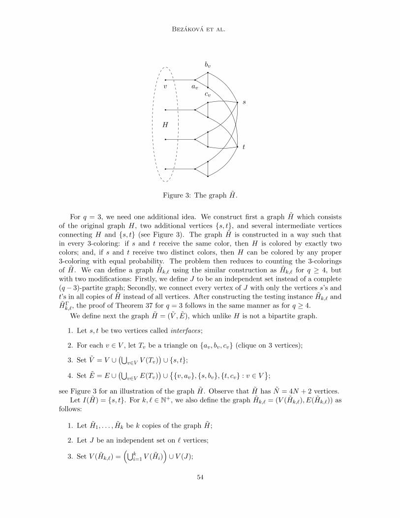
Bezakova et al.

v av

bv

cv

t

s

H

Figure 3: The graph H.

For q = 3, we need one additional idea. We construct first a graph H which consistsof the original graph H, two additional vertices s, t, and several intermediate verticesconnecting H and s, t (see Figure 3). The graph H is constructed in a way such thatin every 3-coloring: if s and t receive the same color, then H is colored by exactly twocolors; and, if s and t receive two distinct colors, then H can be colored by any proper3-coloring with equal probability. The problem then reduces to counting the 3-coloringsof H. We can define a graph Hk,` using the similar construction as Hk,` for q ≥ 4, butwith two modifications: Firstly, we define J to be an independent set instead of a complete(q− 3)-partite graph; Secondly, we connect every vertex of J with only the vertices s’s andt’s in all copies of H instead of all vertices. After constructing the testing instance Hk,` andHΓk,`, the proof of Theorem 37 for q = 3 follows in the same manner as for q ≥ 4.

We define next the graph H = (V , E), which unlike H is not a bipartite graph.

1. Let s, t be two vertices called interfaces;

2. For each v ∈ V , let Tv be a triangle on av, bv, cv (clique on 3 vertices);

3. Set V = V ∪(⋃

v∈V V (Tv))∪ s, t;

4. Set E = E ∪(⋃

v∈V E(Tv))∪v, av, s, bv, t, cv : v ∈ V

;

see Figure 3 for an illustration of the graph H. Observe that H has N = 4N + 2 vertices.Let I(H) = s, t. For k, ` ∈ N+, we also define the graph Hk,` = (V (Hk,`), E(Hk,`)) as

follows:

1. Let H1, . . . , Hk be k copies of the graph H;

2. Let J be an independent set on ` vertices;

3. Set V (Hk,`) =(⋃k

i=1 V (Hi))∪ V (J);

54


4. In addition to the edges in Hi for 1 ≤ i ≤ k, E(Hk,`) also contains edges betweenthe interfaces of Hi for 1 ≤ i ≤ k and every vertex in J ; i.e., for I(Hi) = si, ti andv ∈ J , we have si, v, ti, v ∈ E(Hk,`).

Finally, we define the graph HΓk,` where Γ = m, 3, t in the same way as for q ≥ 4;

namely, we replace every vertex of Hk,` by a copy of the graph G(m, 3, t) and every edgeby an edge between two (unused) ports of the corresponding two gadgets. Furthermore, tomake the graph HΓ

k,` well-defined, we set

m = kN + ` = k(4N + 2) + ` and t = d√qe = 2.

Let B be a complete bipartite graph with the same vertex bipartition as H. By settingH = B, we also define the graphs Bk,` and BΓ

k,`. Given k, ` ∈ N+, let G = HΓk,` and

G∗ = BΓk,`. Suppose d ≥ dc(3) = 4. Then, Lemma 39 implies that G,G∗ ∈M(n, d) for

n = (kN + `) · 4m = 4m2.

The next two lemmas will play the role of Lemmas 41 and 42 in the proof of Theorem 37for the case q = 3.

Lemma 49 Let k, ` ∈ N+ with ` ≥ 2. Then the following holds:

1. If Z3(H) < 2`/k − 2, then

‖µG − µG∗‖tv ≤ 2

(Z3(H) + 2

2`/k

)k.

2. If Z3(H) ≥ 2`/k − 2, then


2

(1−

(Z3(B) + 2

Z3(H) + 2

)k).

Lemma 50 There exists an algorithm with running time O(n) that generates a samplefrom the distribution µG∗.

With these two lemmas in hand, the proof of Theorem 37 for q = 3 is then identical tothat for the q ≥ 4 case and is thus omitted.

7.5.1. Colorings of G and G∗: Proof of Lemmas 49 and 50

It remains for us to prove Lemmas 49 and 50. First, we establish several facts aboutthe 3-colorings of G = HΓ

k,` and G∗ = BΓk,`. We then use these facts as basis to bound

‖µG − µG∗‖tv (Lemma 49) and give a sampling algorithm for µG∗ (Lemma 50). Some ofthese facts are counterparts of those established in Section 7.4.1 for q ≥ 4.

Let Z3(H) denote the number of 3-colorings of H. For i, j ∈ 1, 2, 3, let Zi,j3 (H) be thenumber of 3-colorings of H such that s receives color i and t receives color j.

55

Bezakova et al.

Lemma 51 For i, j ∈ 1, 2, 3, Zi,i3 (H) = 2N+1 and Zi,j3 (H) = 2NZ3(H) when i 6= j.

Proof We first compute Z1,13 (H). Suppose that both s and t are colored with color 1.

Then, for each v ∈ V , colors 2 and 3 are both required to color bv and cv. As a result, avreceives color 1 and v can not be colored by 1 for all v ∈ V . Hence, the vertices of H in Hcan only be assigned colors 2 or 3. There are only two ways to color the connected bipartitegraph H with two colors. This gives

Z1,13 (H) = 2 · 2N = 2N+1,

and by symmetry Z2,23 (H) = Z3,3

3 (H) = 2N+1.

We compute next Z1,23 (H). Let σ be any 3-coloring of H. We claim that there are 2N

colorings of H in which s is assigned color 1, t is assigned color 2, and σ is the coloring inH. From this, it follows immediately that

Z1,23 (H) = 2NZ3(H).

Let v ∈ V and consider 3-colorings of the triangle Tv. If σ(v) = 1, then the only 3-coloringsof the triangle (av, bv, cv) are (2, 3, 1) and (3, 2, 1) since v, av, s, bv and t, cv are alledges of H. Similarly, when σ(v) = 2 or σ(v) = 3, there are also two possible colorings for(av, bv, cv) in each case. Therefore, if s and t are assigned colors 1 and 2 respectively, and σis the coloring in H, there are exactly two proper 3-colorings of Tv for each v ∈ V . As thetriangles Tv are disjoint for v ∈ V , once the colors of s, t and H are assigned, there are 2N

proper 3-colorings of H. This proves our claim, and by symmetry, for any i, j ∈ 1, 2, 3with i 6= j, we obtain Zi,j3 (H) = 2NZ3(H).

As in Lemma 46, we can partition the 3-colorings of Hk,` into two categories.

Lemma 52 Let k, ` ∈ N+. Let Ωa and Ωb be the set of 3-colorings of Hk,` in which J iscolored by exactly 1 and 2 colors respectively. Then Ωa,Ωb is a partition for the set of3-colorings of Hk,`; moreover,

|Ωa| = 3 · 2k(N+1)(Z3(H) + 2)k and |Ωb| = 3 · (2` − 2)2k(N+1).

Proof Observe that in every 3-coloring of Hk,` the number of colors we can assign to theindependent set J is at least one and at most two, since all the vertices of J have at leastone common neighbor. It follows immediately that Ωa,Ωb is a partition for the set of3-colorings of Hk,`. For the 3-colorings in Ωa, we first assign a color to J , say color 1. Then,we count the number of 3-colorings of each Hi whose interfaces si, ti cannot be assignedcolor 1. Lemma 51 and symmetry imply

|Ωa| = 3(Z2,2

3 (H) + Z2,33 (H) + Z3,2

3 (H) + Z3,33 (H)

)k= 3 · 2k(N+1)(Z3(H) + 2)k.

For 3-colorings in Ωb, we pick the two colors that color J , say color 1 and 2. Then, theinterfaces of Hi have to be assigned color 3 for each i. The number of ways to color J withboth colors 1 and 2 is 2` − 2. Then, by Lemma 51 and symmetry, we get

|Ωb| = 3 · (2` − 2)Z3,33 (H)k = 3 · (2` − 2)2k(N+1).

56


Lemma 53 Let σ be a 3-coloring of HΓk,` and τ be the phase vector of σ. Then, τ is a

3-coloring of Hk,`. Moreover, if τ is a 3-coloring of Hk,`, then there are 2m2

3-colorings ofHΓk,` whose phase vector is τ .

Proof The proof is analogous to that of Lemma 47.

Lemma 54 Let k, ` ∈ N+. Let ΩA and ΩB be the set of 3-colorings of HΓk,` whose phase

vector is a 3-coloring of Hk,` that belongs to Ωa and Ωb respectively. Then ΩA,ΩB is apartition for the set of 3-colorings of HΓ

k,`; moreover,

|ΩA| = |Ωa| · 2m2= 3 · 2k(N+1)(Z3(H) + 2)k · 2m2

, and

|ΩB| = |Ωb| · 2m2= 3 · (2` − 2)2k(N+1) · 2m2

.

Proof Follows immediately from Lemmas 52 and 53.

Proof of Lemma 49 We use the notation from the proof of Lemma 41. Following thederivation of (28), we get

‖µG − µG∗‖tv =|ΩAG| − |ΩA

G∗ ||ΩAG|+ |ΩB

G|.

If Z3(H) < 2`/k − 2, then we deduce from Lemma 54 that

‖µG − µG∗‖tv ≤|ΩAG|

|ΩBG|

=3 · 2k(N+1)(Z3(H) + 2)k · 2m2

3 · (2` − 2)2k(N+1) · 2m2

≤ (Z3(H) + 2)k

2`−1= 2

(Z3(H) + 2

2`/k

)k.

If Z3(H) ≥ 2`/k − 2, then by Lemma 54

|ΩAG| = 3 · 2k(N+1)(Z3(H) + 2)k · 2m2 ≥ 3 · 2k(N+1)2` · 2m2 ≥ |ΩB

G|.

Thus, we get

‖µG − µG∗‖tv ≥|ΩAG| − |ΩA

G∗ |2|ΩA

G|=

1

2

(1−|ΩAG∗ ||ΩAG|

)=

1

2

(1−

(Z3(B) + 2

Z3(H) + 2

)k).

Proof of Lemma 50 This can be done in the same way as the proof of Lemma 42. Itsuffices to first generate a random 3-coloring τ of Bk,` and then sample from µG∗ given τas the phase vector where G∗ = BΓ

k,`. To sample a random 3-coloring of Bk,`, we do thefollowing:

1. Compute |Ωa|, |Ωb| and |Ω| = |Ωa|+ |Ωb|;

2. With probability |Ωa|/|Ω| generate a random 3-coloring from Ωa;

57

Bezakova et al.

3. With probability |Ωb|/|Ω| generate a random 3-coloring from Ωb.

We can compute |Ωa| and |Ωb| by Lemma 52. To sample from Ωa, we first pick one colorfor J and then color each copy of B. Notice that since B is a complete bipartite graph, wecan sample a random 3-coloring of B, and consequently B, in linear time. To sample fromΩb, we pick two colors to color J ; then in every copy of B, the complete bipartite graph Bwill receive only two colors. The total running time for sampling a random 3-coloring ofBk,` is O(kN + `) and the running time for sampling from µG∗ is O(n).

8. Discussion

Our hardness results for identity testing for the Ising model require |β|d ≥ c log n for asuitable constant c > 0. We further assume that β∗ = β; namely, our lower bounds holdeven under this additional promise. Our proof extends without any significant modificationto the case where max|β|, |β∗| · d ≥ c log n. As mentioned, there are polynomial runningtime algorithms for identity testing when either |β∗|d = O(log n), in which case we can usestructure learning methods, or when |β| = O(d−1) is in the tree uniqueness region, andknown sampling methods can be combined with the testing algorithm in (Daskalakis et al.,2018). Therefore, when β is the non-uniqueness region (|β|d < c log n) and |β∗|d = ω(log n),the computational complexity of identity testing is open, as there is no known polynomialrunning time algorithm, and our lower bound does not apply to this regime of parameters.

Acknowledgments

Research supported in part by NSF grants 1819546, CCF-1850443, CCF-1617306, CCF-1563838 and CCF-1563757.

References

D.H. Ackley, G.E. Hinton, and T.J. Sejnowski. A Learning Algorithm for Boltzmann Ma-chines. Cognitive Science, 9(1):147–169, 1985.

A. Anandkumar, D.J. Hsu, F. Huang, and S.M. Kakade. Learning mixtures of tree graphicalmodels. In Advances in Neural Information Processing Systems (NeurIPS), pages 1052–1060, 2012.

T. Batu, E. Fischer, L. Fortnow, R. Kumar, R. Rubinfeld, and P. White. Testing ran-dom variables for independence and identity. In Proceedings of the 42nd Annual IEEESymposium on Foundations of Computer Science (FOCS), pages 442–451, 2001.

A. Blanca, Z. Chen, D. Stefankovic, and E. Vigoda. Structure Learning of H-colorings. InProceedings of the 29th International Conference on Algorithmic Learning Theory (ALT),volume 83, pages 152–185, 2018.

A. Bogdanov, E. Mossel, and S. Vadhan. The Complexity of Distinguishing Markov RandomFields. In A. Goel, K. Jansen, J.D.P Rolim, and R. Rubinfeld, editors, Approximation,

58


Randomization and Combinatorial Optimization. Algorithms and Techniques, pages 331–342, Berlin, Heidelberg, 2008. Springer Berlin Heidelberg. ISBN 978-3-540-85363-3.

G. Bresler. Efficiently learning Ising models on arbitrary graphs. In Proceedings of the 47thAnnual ACM Symposium on Theory of Computing (STOC), pages 771–782, 2015.

G. Bresler, E. Mossel, and A. Sly. Reconstruction of Markov random fields from samples:some observations and algorithms. SIAM Journal on Computing, 42(2):563–578, 2013.

G. Bresler, D. Gamarnik, and D. Shah. Structure learning of antiferromagnetic Ising mod-els. In Advances in Neural Information Processing Systems (NeurIPS), pages 2852–2860,2014a.

G. Bresler, D. Gamarnik, and D. Shah. Hardness of parameter estimation in graphicalmodels. In Advances in Neural Information Processing Systems (NeurIPS), pages 1062–1070, 2014b.

G. Brito, I. Dumitriu, and K.D. Harris. Spectral gap in random bipartite biregular graphsand its applications. ArXiv preprint ArXiv:1804.07808, 2018.

A.A. Bulatov, M. Dyer, L.A. Goldberg, M. Jerrum, and C. McQuillan. The expressibilityof functions on the Boolean domain, with applications to Counting CSPs. Journal of theACM (JACM), 60(5):32, 2013.

J.-Y. Cai, A. Galanis, L.A. Goldberg, H. Guo, M. Jerrum, D. Stefankovic, and E. Vigoda.#BIS-hardness for 2-spin systems on bipartite bounded degree graphs in the tree non-uniqueness region. Journal of Computer and System Sciences, 82(5):690–711, 2016.

C. Calabro, R. Impagliazzo, V. Kabanets, and R. Paturi. The complexity of Unique k-SAT: An Isolation Lemma for k-CNFs. Journal of Computer and System Sciences, 74(3):386–393, 2008.

C.L. Canonne, I. Diakonikolas, T. Gouleakis, and R. Rubinfeld. Testing Shape Restrictionsof Discrete Distributions. Theory of Computing Systems, 62(1):4–62, 2018.

X. Chen, M. Dyer, L.A. Goldberg, M. Jerrum, P. Lu, C. McQuillan, and D. Richerby.The complexity of approximating conservative counting CSPs. Journal of Computer andSystem Sciences, 81(1):311–329, 2015.

C.K. Chow and C. Liu. Approximating discrete probability distributions with dependencetrees. IEEE Transactions on Information Theory, 14(3):462–467, 1968.

A. Collevecchio, T.M. Garoni, T. Hyndman, and D. Tokarev. The Worm process for theIsing model is rapidly mixing. Journal of Statistical Physics, 164(5):1082–1102, 2016.

S. Dasgupta. Learning polytrees. In Proceedings of the 15th Conference on Uncertainty inArtificial Intelligence (UAI), pages 134–141, 1999.

C. Daskalakis, E. Mossel, and S. Roch. Evolutionary trees and the Ising model on theBethe lattice: a proof of Steel’s conjecture. Probability Theory and Related Fields, 149(1-2):149–189, 2011.

59

Bezakova et al.

C. Daskalakis, N. Dikkala, and G. Kamath. Testing Ising models. In Proceedings of the29th Annual ACM-SIAM Symposium on Discrete Algorithms (SODA), pages 1989–2007,2018.

I. Diakonikolas and D.M. Kane. A new approach for testing properties of discrete distribu-tions. In Proceedings of the 57th Annual IEEE Symposium on Foundations of ComputerScience (FOCS), pages 685–694, 2016.

I. Diakonikolas, D.M. Kane, and V. Nikishkin. Optimal algorithms and lower bounds fortesting closeness of structured distributions. In Proceedings of the 56th Annual IEEESymposium on Foundations of Computer Science (FOCS), pages 1183–1202, 2015.

I. Diakonikolas, T. Gouleakis, J. Peebles, and E. Price. Sample-Optimal Identity Testingwith High Probability. In Proceedings of the 45th International Colloquium on Automata,Languages, and Programming (ICALP), volume 1, pages 1–41, 2018.

M. Dyer, L.A. Goldberg, C. Greenhill, and M. Jerrum. The relative complexity of approx-imate counting problems. Algorithmica, 38(3):471–500, 2004.

M. Dyer, L.A. Goldberg, and M. Jerrum. An approximation trichotomy for Boolean #CSP.Journal of Computer and System Sciences, 76(3-4):267–277, 2010.

T. Emden-Weinert, S. Hougardy, and B. Kreuter. Uniquely colourable graphs and thehardness of colouring graphs of large girth. Combinatorics, Probability and Computing,7(4):375–386, 1998.

J. Felsenstein. Inferring phylogenies, volume 2. Sinauer Associates, Inc., Sunderland, MA,2004.

S. Friedli and Y. Velenik. Statistical mechanics of lattice systems: a concrete mathematicalintroduction. Cambridge University Press, 2017.

A. Galanis, L.A. Goldberg, and M. Jerrum. Approximately Counting H-Colourings is#BIS-Hard. SIAM Journal on Computing, 45(3):680–711, 2016a.

A. Galanis, D. Stefankovic, and E. Vigoda. Inapproximability of the partition functionfor the antiferromagnetic Ising and hard-core models. Combinatorics, Probability andComputing, 25(4):500–559, 2016b.

S. Geman and C. Graffigne. Markov random field image models and their applicationsto computer vision. In Proceedings of the International Congress of Mathematicians,volume 1, pages 1496–1517. Berkeley, CA, 1986.

H.-O. Georgii. Gibbs measures and phase transitions, volume 9. Walter de Gruyter, 2011.

L.A. Goldberg and M. Jerrum. The complexity of ferromagnetic Ising with local fields.Combinatorics, Probability and Computing, 16(1):43–61, 2007.

L.A. Goldberg and M. Jerrum. Approximating the partition function of the ferromagneticPotts model. Journal of the ACM, 59(5):25, 2012.

60


L.A. Goldberg and M. Jerrum. Approximating pairwise correlations in the Ising Model.ACM Transactions on Computation Theory. To appear, 2019.

O. Goldreich, S. Goldwasser, and D. Ron. Property testing and its connection to learningand approximation. Journal of the ACM, 45(4):653–750, 1998.

H. Guo and M. Jerrum. Random cluster dynamics for the Ising model is rapidly mixing. InProceedings of the 28th Annual ACM-SIAM Symposium on Discrete Algorithms (SODA),pages 1818–1827, 2017.

L. Hamilton, F. Koehler, and A. Moitra. Information theoretic properties of Markov randomfields, and their algorithmic applications. In Advances in Neural Information ProcessingSystems (NeurIPS), pages 2460–2469, 2017.

S. Hoory, N. Linial, and A. Wigderson. Expander graphs and their applications. Bulletinof the American Mathematical Society, 43(4):439–561, 2006.

R. Impagliazzo and R. Paturi. On the Complexity of k-SAT. Journal of Computer andSystem Sciences, 62(2):367–375, 2001.

M. Jerrum and A. Sinclair. Polynomial-time approximation algorithms for the Ising model.SIAM Journal on computing, 22(5):1087–1116, 1993.

A. Klivans and R. Meka. Learning graphical models using multiplicative weights. In Pro-ceedings of the 58th Annual Symposium on Foundations of Computer Science (FOCS),pages 343–354. IEEE, 2017.

K.-I. Ko. Some observations on the probabilistic algorithms and NP-hard problems. Infor-mation Processing Letters, 14(1):39–43, 1982.

S.-I. Lee, V. Ganapathi, and D. Koller. Efficient Structure Learning of Markov Networks us-ing L1-Regularization. In Advances in Neural Information Processing Systems (NeurIPS),pages 817–824, 2007.

M. Molloy and B. Reed. Colouring graphs when the number of colours is nearly the maxi-mum degree. In Proceedings of the 33rd Annual ACM Symposium on Theory of Computing(STOC), pages 462–470, 2001.

D. Randall and D. Wilson. Sampling spin configurations of an Ising system. In Proceedingsof the 10th Annual ACM-SIAM Symposium on Discrete Algorithms (SODA), pages 959–960, 1999.

P. Ravikumar, M.J. Wainwright, and J.D. Lafferty. High-dimensional Ising model selectionusing `1-regularized logistic regression. The Annals of Statistics, 38(3):1287–1319, 2010.

S. Roth and M.J. Black. Fields of experts: A framework for learning image priors. InProceedings of the 2005 IEEE Computer Society Conference on Computer Vision andPattern Recognition (CVPR), volume 2, pages 860–867, 2005.

R. Rubinfeld and M. Sudan. Robust characterizations of polynomials with applications toprogram testing. SIAM Journal on Computing, 25(2):252–271, 1996.

61

Bezakova et al.

R. Salakhutdinov and G. Hinton. An efficient learning procedure for Deep BoltzmannMachines. Neural Computation, 24(8):1967–2006, 2012.

R. Salakhutdinov and H. Larochelle. Efficient learning of deep Boltzmann machines. InProceedings of the 13th International Conference on Artificial Intelligence and Statistics(AISTATS), pages 693–700, 2010.

N.P. Santhanam and M.J. Wainwright. Information-theoretic limits of selecting binarygraphical models in high dimensions. IEEE Trans. Information Theory, 58(7):4117–4134,2012.

A. Sly. Computational transition at the uniqueness threshold. In Proceedings of the 51stAnnual IEEE Symposium on Foundations of Computer Science (FOCS), pages 287–296,2010.

A. Sly and N. Sun. The computational hardness of counting in two-spin models on d-regulargraphs. In Proceedings of the 53rd Annual Symposium on Foundations of ComputerScience (FOCS), pages 361–369, 2012.

G. Valiant and P. Valiant. An automatic inequality prover and instance optimal identitytesting. SIAM Journal on Computing, 46(1):429–455, 2017.

M. Vuffray, S. Misra, A. Lokhov, and M. Chertkov. Interaction screening: Efficient andsample-optimal learning of Ising models. In Advances in Neural Information ProcessingSystems (NeurIPS), pages 2595–2603, 2016.

M. Vuffray, S. Misra, and A.Y. Lokhov. Efficient Learning of Discrete Graphical Models.ArXiv preprint ArXiv:1902.00600, 2019.

S. Wu, S. Sanghavi, and A.G. Dimakis. Sparse logistic regression learns all discrete pairwisegraphical models. In Advances in Neural Information Processing Systems (NeurIPS),pages 8069–8079, 2019.

62

Documents

Lower Bounds for Testing Graphical Models: Colorings and