Low-income before and after Housing Costs, Comparing Australia’s Regions

Paper prepared for the Australian Social Policy Conference, 2003

by Peter Siminski and Peter Saunders, Social Policy Research Centre

2

1 Introduction

This paper is part of a broader project on household inequality and living standards being conducted by the Social Policy Research Centre in partnership with the Australian Bureau of Statistics under an ARC Linkage grant. The paper expands on and extends some of the findings made by Siminski and Norris (2003), recently published in Australian Social Trends. The main purpose of the paper is to discuss methodological issues in assessing geographical differences in the propensity of households to be relatively poor, and to make a broad assessment of such geographical differences.

An issue of particular significance is the way in which differences in housing costs between regions should be addressed in the analysis. The use of a standard ‘disposable income’ measure yields very different results to an ‘income after housing costs’ measure. It is argued that the latter is a useful alternative indicator of comparative living standards, though both measures have their limitations.

The major issues regarding comparisons of household income between regions are discussed in Section 2, and a new framework for addressing differences in housing costs is presented. A comparison of the ‘after housing’ and ‘imputed rent’ approaches to accounting for housing is made in Section 3. Section 4 summarises the methods used in this paper, while Section 5 presents the results. Section 6 offers conclusions.

3

2 Analysing Regional Differences in Household Income

Income is only a limited indicator of relative living standards. In fact, recent studies of measuring ‘direct utility’ indicate that if there is any relationship between income and happiness, then it is only weak. Happiness is linked much more strongly with other factors such as the quality of personal relationships and employment stability (Hamilton, 2003). More complete analyses of regional disparities in living standards and well-being would consider differences in health outcomes, crime, local economic stability, social capital, time stress, access to goods and services and many other factors, such as those presented by Bray (2001). Therefore, it is important to emphasise that this study does not aim to be conclusive on the issue of well-being.

Nevertheless, most people would agree that regional disparities in income are interesting in their own right, and we believe that there is scope for the development of measures in this domain. There have been few attempts to analyse differences in household income between broad geographical areas similar to that undertaken in the present study. One recent such study by Lloyd, Harding and Hellwig (2001) concluded that there is a ‘large and growing gap between the incomes of those Australians living in capital cities and those living in the rest of Australia’. But the authors acknowledge that their study did not take into account any regional price differences. This is understandable, since no comprehensive indices of regional price differences exist in Australia. However, such price differences can be significant particularly in relation to housing (see for example King, 1995), thus questioning the value of simple income comparisons and their conclusions. Bray (2001) shows that the proportion of households that have ‘lower income’1 is much higher in areas outside of capital cities, but he too does not consider differences in prices or housing costs. Harding and Szukalska (2000) compare poverty rates between capital cities and the rest of Australia, before and after housing costs. Their results indicate that the difference in poverty rates between capital cities and the rest of Australia changes little between the before and after housing costs measures, a finding that is very different to the results presented in this paper (although the methods are not strictly comparable).

Citro and Michael (1995: 182-201), discuss the issue of adjustments to the poverty threshold on the basis of price differentials by geographical area, in the context of measuring poverty in the US. They show that there is a significant literature devoted to this issue, and that the task is very complex. Numerous issues arise such as whether the adjustment should be made on the basis of a fixed bundle of goods and services, or a regionally specific bundle. Should this bundle be based on an average household’s consumption bundle (such as the CPI bundle), or a relatively poor household’s consumption bundle? Since any such an index would assume uniformity within a given region, how large or small should each region under consideration be? They argue that even though these issues pose considerable challenges, the task is worth pursuing. They argue that a bundle of goods and services which is typical of a low income household and

1 He defines lower income as being in the bottom 43.2 per cent of the income distribution.

4

fixed across regions should be priced in different geographical areas, and income should be adjusted accordingly. In the spirit of this approach, it would be possible to develop an index for Australia’s regions using the bundle of goods and services established by the SPRC’s budget standards research (Saunders et al., 1998). See Saunders (1998) for a start in this direction.

However, one issue that has been somewhat neglected by such research is the specific nature of housing within the consumption bundle. A washing machine purchased in the country is the same commodity as an identical washing machine purchased in the city and both provide identical services, so comparing their prices is a sensible exercise. Housing, however, can not be assumed to be a homogenous commodity across regions. Consider an apartment in the city and one in the country. Even if the dwellings themselves are physically identical, their location makes them fundamentally different commodities in terms of the services they provide, rather than the same commodity at a different price. For related reasons, the literature on cross-country income comparisons acknowledges difficulties in accounting for housing in the construction of Purchasing Power Parities (PPPs), referring to housing as ‘comparison resistant goods’ (Castles, 1997: 28).

An important question to address is why the market will usually value the dwelling in the city at a higher price. There are two apparent possible reasons for this. Firstly, it is possible that people prefer to live in cities than in the country, for reasons of accessibility to shopping, leisure facilities, or to other people. If this was the entire reason for the price differentials, then there should be no need to make price adjustments between regions on the basis of housing. Housing could be seen as consumption expenditure, and the choice of a location of residence would reflect consumption preferences.

An alternate explanation for the city-country differential in housing prices is to consider the geographical location of paid work, and wage differentials between regions. Since at least the industrial revolution, remuneration of paid work has been generally higher in urban areas than in regional or remote areas. The choice of where to live is also constrained on the basis of where jobs are available. It is reasonable to assume that people would consider both their potential income and their housing costs in assessing where to live.2 The difference between the price of an apartment in the city and an identical apartment in the country could largely be considered as an expense associated with earning a higher income in the city. Under this reasoning, it would make sense for regional comparisons of income to be made net of the premium in housing costs that result from such labour market issues. Such an approach implies adjusting the definition of income, whilst regarding housing in different regions to be different commodities. The standard approach on the other hand, as described by Citro and Michael, is to treat housing in different locations to be the same commodity at different prices, and hence not adjusting the definition of income, but only its value.

2 This choice is constrained, however, since regional differences in earnings are partly driven by regional

differences in industrial and occupational structure.

5

In recent years, there has been a net internal migration out of major cities in Australia, mostly of low-income people (Marshall et al., 2003), who have been ‘pushed out’ of the cities by rising housing prices. Under the framework described above, they could be regarded to have moved in order to maximise their income net of housing costs. Of course such a framework ignores any non-monetary benefits of living in a given area, as discussed above. Marshall et al.’s (2003) work suggests that this migration should be considered in a broader context than as involuntary relocation. However, the lack of affordable housing in large cities is the main reason for such migration.

In order to adopt this framework, one would need to disaggregate each household’s housing expenses into a ‘work expense’ component associated with location, and a consumption component (consisting of the benefits of the physical dwelling itself and the consumption benefits of the location). A stylised example of how such components may differ geographically is shown in Figure 1. In this hypothetical example, three dwellings are considered. These are located in a remote, a regional, and a city area, respectively but are otherwise identical. The consumption value of the dwelling (in terms of the services it guarantees) is constant across regions. The consumption value of the location is assumed to be higher in the city in this example, but this may not necessarily reflect reality, and would vary between and within regions. For example, this component would probably be very high for a house by a beach in a major city, and much lower for a house in the same city located in a less appealing location. The ‘work expense’ component of the cost of housing is assumed to be strongly related to location, being much higher in the city than elsewhere, and nil in rural areas. Under the framework proposed here, one should subtract the ‘location (work expense)’ component of housing consumption from each household’s income in order to make meaningful comparisons between regions.

6

Figure 1 Stylised example of the determinants of housing price differences between regions

It may be possible to adopt this framework comprehensively, utilising detailed housing and wage data, though this is beyond the scope of this paper. However, this framework points to an alternate (available) method, in which all three components of housing costs discussed above are subtracted from income. This is a reasonable method to adopt if one assumes that the ‘location (consumption)’ component is a small determinant of housing cost differences, and if the quality of dwellings is not systematically different between the regions under consideration. These are non-trivial assumptions. At the very least, the after housing costs method provides a useful measure to complement comparisons of income before housing costs.

In comparing incomes between regions, the after housing costs method ignores housing quality (which may vary between regions), while the before housing costs method ignores house prices (which vary greatly between regions).

Remote Regional City

location (work expense)location (consumption)dwelling (consumption)

7

3 Income after Housing Costs versus Imputed Rent

There are two main approaches that have been used to account for housing costs in studies of income distribution: imputing rent to owner-occupiers, or subtracting housing costs from all households. These are very different methods, but there are advantages and disadvantages to both. A comprehensive treatment of the differences in the two methods is beyond the scope of the paper. However, a summary of some of the main differences is presented here, with a focus on regional issues. We argue that imputing rent does not resolve the issue of differing housing prices between city and regional areas, while an after-housing costs measure does.

There has been a strong case made for imputing rent to the income of owner occupiers for many forms of analysis. Cash income is not a good indicator of the well being of (outright) home owners in relation to renters of dwellings, because the former have no rent to pay. There is a non-cash income simultaneously earned and spent by the home-owner, an income that is a return on the housing asset. Imputing rent overcomes this issue directly by treating owner-occupiers as if they were renting their home from themselves. It includes such rent (net of operating expenses such as maintenance and council and water rates) as a form of income, thus creating an income measure that is comparable between owner-occupiers and renters. This approach also includes the value of housing assistance provided to public renters (defined as the difference between the ‘market rent’ of the dwelling and the rent actually charged) as a component of their income. This is referred to as the ‘market value’ approach to imputing rent. Other methods also exist, such as the ‘opportunity cost approach’ which considers how much income a household would be earning if it was to invest its housing equity in financial assets, which is the cash income foregone by the decision to be an owner-occupier.

Imputing rent is a powerful method of creating a more comprehensive income measure that is comparable across households of different housing tenure. In Australia, the most significant work in developing this approach has been undertaken by Yates (1991; 1994), and it has also been utilised by Travers and Richardson (1993). Whiteford and Kennedy (1995) have used this approach in making cross-national comparisons of the living standards of older people. The Canberra Group (2001: 62) suggests that a measure of income that includes imputed rent will produce a ‘fairer and more accurate picture of income distribution’ for the purposes of international comparisons.

However, the method of imputing rent necessitates the assumption that housing is purely a consumption good. It takes no account of differences in the cost of housing between regions. As discussed in Section 2, there is a strong argument for treating the additional cost of housing in urban areas (as compared to rural areas) not as additional consumption, but as an expense associated with earning a higher income.

Futhermore, the income of private renters is unchanged between the cash income method and the imputed rent method, since they do not own their homes. Consider the hypothetical case of two identical families who earn identical incomes and live in identical dwellings (one in the city and one in the country), for which the family in the city pays a higher rent. The imputed rent approach leads to the same conclusion as the

8

cash income approach, that the two families experience the same level of material well-being. Clearly, however, the family living in the country is materially ‘better off’ than the family in the city (as indicated by an after housing costs measure of income), assuming that the prices and availability of other goods and services do not vary sufficiently to change this conclusion. A similar argument could also be made for home purchasers, although complications arise if one considers the effect of capital gains.

The after-housing costs measure, on the other hand, indirectly controls for price differences between regions, as discussed in Section 2 and acknowledged by the Commission of Inquiry into Poverty (1975: 149) and Bradbury, Rossiter and Vipond (1986: 11), though little emphasis has been placed on the results of comparisons made between regions using this method. The after-housing costs measure has also been regularly used to control for differences between owners, purchasers and renters (Commission of Inquiry into Poverty, 1975; Bradbury, Rossiter and Vipond, 1986; Harding and Szukalska, 2000; Saunders, 1994?#), although the imputed rent method is usually regarded as a preferable method for the latter purpose (Bradbury, Rositter and Vipond, 1986: 10) since housing quality is implicitly taken into account (albeit only as implied by its monetary value).

In the comparative social policy literature, Ritakallio (2003: 89) compares the after-housing costs measure to the before housing costs measure and the imputed rent measure. He argues that the former ‘most genuinely reflects the daily life situation when households are assessing the sufficiency or insufficiency of their disposable incomes’. He also argues that income after housing costs should be the standard basis for making cross-national comparisons of poverty (p.99). We stop short of making the same claim for the use of income after-housing costs for intra-national comparisons of living standards between regions. Nevertheless, income after housing costs has some characteristics that make it preferable to the other two measures of income for analysing differences between regions in the propensity of people to be relatively poor.

9

4 Data and Methods

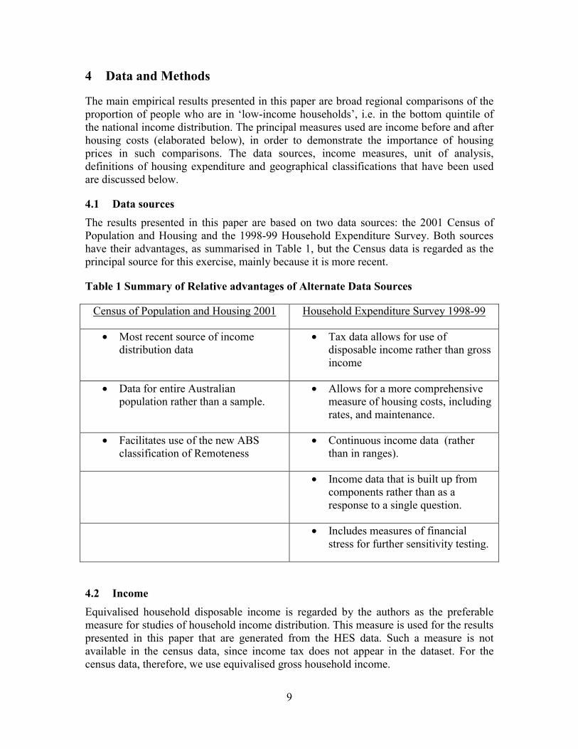
The main empirical results presented in this paper are broad regional comparisons of the proportion of people who are in ‘low-income households’, i.e. in the bottom quintile of the national income distribution. The principal measures used are income before and after housing costs (elaborated below), in order to demonstrate the importance of housing prices in such comparisons. The data sources, income measures, unit of analysis, definitions of housing expenditure and geographical classifications that have been used are discussed below.

4.1 Data sources The results presented in this paper are based on two data sources: the 2001 Census of Population and Housing and the 1998-99 Household Expenditure Survey. Both sources have their advantages, as summarised in Table 1, but the Census data is regarded as the principal source for this exercise, mainly because it is more recent.

Table 1 Summary of Relative advantages of Alternate Data Sources

Census of Population and Housing 2001 Household Expenditure Survey 1998-99

• Most recent source of income distribution data

• Tax data allows for use of disposable income rather than gross income

• Data for entire Australian population rather than a sample.

• Allows for a more comprehensive measure of housing costs, including rates, and maintenance.

• Facilitates use of the new ABS classification of Remoteness

• Continuous income data (rather than in ranges).

• Income data that is built up from components rather than as a response to a single question.

• Includes measures of financial stress for further sensitivity testing.

4.2 Income Equivalised household disposable income is regarded by the authors as the preferable measure for studies of household income distribution. This measure is used for the results presented in this paper that are generated from the HES data. Such a measure is not available in the census data, since income tax does not appear in the dataset. For the census data, therefore, we use equivalised gross household income.

10

The person is the unit of analysis, and it is assumed that income is shared fairly within the household. In other words, we use ‘person-weighted’ household income for both the census and HES data.

The equivalence scales adopted are the Henderson equivalence scales, since they explicitly differentiate between the equivalence adjustments required for disposable income, and for disposable income after housing costs.

Whilst for many purposes, annual income is often regarded as a preferable measure to current (weekly) income, the latter is the only measure available in the Census and in the HES data.

In the HES data, sensitivity tests were conducted to determine whether the exclusion of households with nil or negative incomes makes a significant difference to the results. These exclusions did not make a significant difference, as shown in Appendix 1.

4.3 Expenditure on Housing The choice of the appropriate measure of housing costs is non-trivial, it depends on the focus of the study and it is limited by available data. This measure should be defined in a way such that households of different tenure types are treated comparably. Rent payments are the only housing costs included for renters. Since rent payments cover the landlord’s council rates, water rates, maintenance costs and building insurance, for consistency these should be included in the housing costs of owner-occupiers, who directly incur such costs.

The question of whether or not to include the principal component of mortgage repayments as part of housing expenditure is less simple. The argument against inclusion is that this can be considered as saving or investment, hence representing a voluntary choice on behalf of the owner-occupier to defer consumption. The argument for inclusion is that the resulting measure of income after housing is the better indicator of income available for non-housing consumption. We prefer to include payments on the principal component for this reason. This is also clearly the better measure in the case of children, since the deferral of consumption is not a choice that they are likely to contribute to, and they are less likely than their parents to benefit from such saving when it is realised in the future. Bradbury and Jantti (1999: 6) make a similar point in arguing that the savings component of household income is not a contributor to children’s consumption.

Therefore, the preferred measure of expenditure on housing is the sum of current (direct) housing costs (consisting of rent, mortgage repayments – interest component, general rates, house and contents insurance, repairs and maintenance, loans for alterations and additions – interest component, and body corporate payments) and the principal component of mortgage repayments. This is the measure used in the results derived from the HES data. Again, the census data is rather more limited in the choice of a housing expenditure variable. The only measure of housing expenditure in the Census data includes rent, (total) mortgage payments, and site fees if the dwelling is a caravan or a manufactured home in a caravan park or manufactured home estate.

11

In the HES data, sensitivity tests were conducted to determine whether the three measures of housing costs discussed above (current housing costs; current housing costs plus the principal component of mortgage repayments; and the census version of housing expenditure) produce significantly different results. These variations did not make a significant difference, as shown in Appendix 1.

4.4 Indicators of Financial Stress We also present some results using the HES indicators of financial stress to complement the low income before and after housing costs analysis. The question addressed is whether having a low income corresponds differently to financial stress between geographical areas. We use fourteen of the sixteen indicators of financial stress included in the HES data set. These are:

• Unable to raise $2000 in a week for something important;

• Could not pay electricity, gas or telephone bills on time;

• Could not pay car registration or insurance on time;

• Pawned or sold something;

• Went without meals;

• Could not afford to heat home;

• Sought assistance from welfare/community organisations;

• Sought financial help from friends or family;

• Could not afford a holiday for at least one week a year;

• Could not afford a night out once a fortnight;

• Could not afford friends or family over for a meal once a month;

• Could not afford a special meal once a week;

• Could only afford second hand clothes most of the time;

• Could not afford leisure or hobby activities.

We consider households that report two or more forms of financial stress to be ‘financially stressed’. We make no attempt, here, to justify the choice of using two, rather than one or three, or another number of financial stress indicators. The focus is on making comparisons between regions, not on asserting what proportion of low-income people are ‘genuinely’ in financial stress.

12

4.5 Geographical Classifications Given that the main focus of the paper is to make broad regional comparisons, the choice of geographical classification is important. We use two geographical classifications, which are defined quite differently. These are the ABS classification of ‘Remoteness’, and the ABS ‘Section of State’ classification. These yield different, though complementary results.

The remoteness classification is a formula-driven classification, based on the physical road-distance from each collection district to the nearest urban centres in each of five size classes. The resulting categorisation is:

• Major Cities of Australia;

• Inner Regional Australia;

• Outer Regional Australia;

• Remote Australia;

• Very Remote Australia;

• and Migratory (a category not considered in this analysis. It is composed of off-shore, shipping and migratory Collection Districts). (ABS, 2002: 37).

The remoteness classification is available for the Census data, but it is not readily available for the HES data.

The Section of State (SOS) classification, on the other hand, is available for both the Census data and the HES data. SOS is defined only in census years, so we have used the 1996 classification for the HES data. Each SOS category represents an aggregation of non-contiguous geographical areas of a particular urban/rural type. These categories are

• Major Urban (urban areas with a population of 100,000 or over);

• Other Urban (urban areas with a population of between 1000 and 99,999 people);

• Bounded Locality (rural localities with populations of between 200 and 999 people);

• Rural Balance (the remainder of the State/Territory);

• Migratory (a category not considered in this analysis. It is composed of off-shore, shipping and migratory Collection Districts). (ABS, 2002: 35).

Despite its name, the Section of State classification does not enforce analysis by State/Territory.

13

These two classifications are quite distinct. Consider, for example, a Census Collection District (CD) that lies between Sydney and Wollongong, and that is not within a town or ‘locality’. This CD would be included in the ‘rural balance’ category in the SOS structure, whilst it would be classified in the ‘inner regional’ category of the Remoteness structure. In fact, the vast majority of the East Coast of Australia between Rockhampton and Melbourne is classified as either Inner Regional or Outer Regional Australia in the Remoteness Structure, whilst any CD outside of bounded urban areas or localities is counted in the ‘rural balance’ of the SOS structure. Importantly, however, the Major Cities category is, in practice, reasonably similar to the Major Urban category. (see ABS, 2001: 20), and so comparisons between the major cities/ major urban areas and the rest of Australia should not be affected to a great degree by which classification is used.

14

5 Results

We have argued that an after housing costs measure of income is useful for comparisons between regions of the propensity for people to be in relatively poor households. We now present results, in three sections. First, we make broad comparisons between major cities/major urban areas and the balance of Australia. (as explained in Section 4.5, ‘major cities’ is a category in the Remoteness classification, whereas ‘major urban’ areas are a category in the Section of State classification). Next we present corresponding results using the more detailed geographical classifications. Finally, we assess the relationship between low-income and financial stress for different regions.

5.1 Major Cities/Major Urban Areas Compared with the Balance of Australia The Census 2001 data suggests that people living in major cities are much less likely to live in low-income households than people living elsewhere in Australia (17 per cent compared with 26 per cent). Similarly, the HES 98-99 data suggests that people living in major urban areas are much less likely to live in low-income households than people living elsewhere in Australia (17 per cent compared with 25 per cent). However, when income after housing is considered, this difference is far smaller. The Census data suggests that the difference narrows to just one percentage point (20 per cent compared with 21 per cent). The HES data suggests that the difference is more like three per cent (19 per cent compared with 22 per cent), a statistically significant difference at the one per cent level. These results are shown in Figure 2. There are many possible reasons for the discrepancy between the Census and HES results that have not been controlled for, as described in Section 4. One possible legitimate reason for the discrepancy, however, is the increase in the cost of housing in major cities between the time of the HES survey, and the Census. For the eight major cities, CPI figures indicate that the price of housing rose by 16.0% between 1998-99 and 2001-02, compared to an increase in the overall CPI of 11.7% (ABS, 2003: Table 28.3). Comparable data are not available for the balance of Australia.

In any case, the main finding emerges from either data source. The income after housing measure suggests that there is a much smaller difference between major cities and the rest of Australia in the proportion of people living in low-income households, as compared to the before housing measure. However, this proportion is still somewhat higher in the balance of Australia than in major cities.

15

Figure 2 People in low-income (first quintile) households before and after housing by major city/major urban versus balance of Australia (per cent)

5.2 Comparisons between more detailed geographical regions When the more detailed classifications of geography are used, a more confusing story emerges. The Census and HES data reveal a paradoxical, though not contradictory, pattern of low income before and after housing costs.

Figure 3 shows the percentage of people in low-income households before and after housing costs by Remoteness. There is a positive relationship between increasing remoteness and the low income before housing rate. However, income after housing indicates a relationship which is largely the opposite – increasing remoteness being associated with a decreasing proportion of people in low-income households, the exception to this relationship being that this rate is higher for Inner regional areas than for Major Cities. Care needs to be taken in interpreting these results because of the discrepancies in the number of people living in each region. Major Cities are dominant (in which 67 per cent of people reside), whilst the corresponding percentages for the other regions are 21, 10, 1.5 and 0.8, respectively. Clearly, the vast majority of people reside in the first three regions. For these three regions, the rate of low income before housing varies from 17 per cent (Major cities) to 27 per cent (Outer regional), while the rates of low income after housing is very much less (ranging from 19 to 22 per cent).

1720

17 19

26

2125

22

0

5

10

15

20

25

30

before HC after HC before HC after HC

Census 2001 HES 98-99

Major cities/major urban balance

16

Figure 3 Percentage of people in low-income households before and after housing by Remoteness – Census 2001

In the HES results that follow, ‘bounded localities’ are grouped with ‘rural balance’, since the sample size of the former is relatively small and because their percentages are generally similar. In the resulting classification, 64 per cent of people are in the ‘major urban’ category, 23 per cent are in the ‘other urban’ category, and 13 per cent are in the ‘rural’ category, which consists of ‘bounded localities’ and the ‘rural balance’.3 These percentages are quite similar to those of the first three categories in the remoteness classification discussed above.

The HES results suggest that the rate of low income before housing is higher for ‘other urban’ areas than for ‘major urban’ areas, and it is higher again for rural areas. This same pattern is also evident for income after housing. All the differences discussed here are statistically significant, with p-values of 5 per cent at most. This analysis will be repeated using Census data, to test its sensitivity to the differences between the two data sources and the available methods of analysis.

3 Referring to this combined category as ‘rural’ is consistent with the section of state classification (ABS,

2002: 35)

17

2427 25

42

2022

1915

13

05

1015202530354045

Major City InnerRegional

OuterRegional

Remote VeryRemote

before HC after HC

17

Figure 4 Percentage of people in low-income households before and after housing by Section of State – HES 98-99

Though this section remains work in progress, we are left with seemingly paradoxical findings. Low-income rates before housing are positively related to remoteness, and negatively related to the size of the town, but there is a more complex story in comparisons of low-income rates after housing. The HES data suggests that the smaller the town or locality, the higher the rate of low-income after housing. The Census data, on the other hand, suggests that (excluding major cities), increasing Remoteness is associated with lower rates of low income after housing, although there is little difference between the three main regional categories. The interim conclusion is that rural areas generally have higher rates of low income after housing than urban areas, but that these rates are actually lower for remote areas. Further work is needed to confirm this conclusion.

5.3 Financial Stress Finally, we consider the relationship between low income (before and after housing) and financial stress. As discussed in Section 4.4, we consider households which have indicated experiencing at least two of the fourteen types of financial stress to be financially stressed.

McColl, et al. (2002) found ‘little difference … in the incidence of all levels of financial stress between households in capital cities, other urban and rural areas within each income grouping’. Using slightly different methods, our results suggest that there is a large difference between urban and rural low-income households in the propensity of financial stress.

17

21

30

1921

24

0

5

10

15

20

25

30

35

Major Urban Other Urban Rural

before HC after HC

18

Figure 5 shows the proportion of people in low-income households that are financially stressed. These rates change very little between the use of income before and after housing. Clearly, this percentage is much lower for rural areas than for the other areas. Less than half of people in low income households in rural areas are financially stressed, while this figure is over 60 per cent in major urban areas, and over two thirds in other urban areas.

Figure 5 Percentage of people in low-income households (before and after housing) that are financially stressed by Section of State – HES 98-99

This may suggest that it is less financially stressful to be in a low-income household in rural areas than urban areas. Alternatively, people living in rural areas may be less likely to admit to financial stress, though this does not seem to be the case given that the proportion of all rural households that are financially stressed is the same as that of households in capital cities.4 These differences could also be associated with regional differences in how poor these relatively poor households are (as in the ‘poverty gap’), or to other characteristics that we haven’t controlled for in the analysis. The difference in these rates between major urban and other urban areas are also statistically significant. We refrain from making any strong conclusions in this section.

4 Calculated from McColl et al. (2002: Table 7)

61 6168 68

45 47

-1020304050607080

before housing after housing

Major Urban Other Urban Rural

19

6 Conclusion

The first main point of this paper has been to argue that simple comparisons of low-income (before housing) rates (or poverty rates defined by a head-count ratio) between Australia’s regions have very limited utility. Differences in prices, especially of housing, are too significant to ignore.

The second main argument concerns what is typically known as ‘housing consumption’. We suggest that a component of such a measure is not consumption at all, but it is actually more akin to a work expense. The higher housing costs of major cities should perhaps be regarded primarily as a cost associated with earning the (typically) higher incomes that are characteristic of such cities. Therefore, in comparing the incomes of households between regions, a more appropriate measure of income would be net of housing cost differences.

The ‘imputed rent’ approach does not resolve the issue of regional price differences. In fact, through its assumption that housing consumption is, in fact, solely consumption, it extenuates the problem of regional housing price differences. Of the available methods of income distribution analysis, the ‘after housing’ measure, on the other hand is the most appropriate for such regional analysis. While the benefits of using an after housing measure for regional comparisons have been acknowledged in the literature, such results have rarely been presented with any conviction.

The main empirical finding reported in this paper suggests that there is only a small difference between major cities and the rest of Australia in the percentage of people living in low-income households after housing. This contrasts with the large difference between major cities and the rest of Australia in the corresponding rates before housing. Another finding is that low-income rates are higher for rural areas than for urban areas, but lower for remote areas. Finally, our results suggest that low-income households located in rural areas are far less likely to report multiple financial stress than households in urban areas, whether income is measured before or after housing.

20

Appendix A Sensitivity tests

The low income rates derived under various alternate definitions are shown in Table A.1. None of the differences between the selected measures and alternate measures are significant at the 10 per cent level of significance. Therefore, the results are not sensitive to the housing expenditure definition, nor to the inclusion or exclusion of households with negative or nil incomes.

Table A. 1 Low income rates by Section of State (HES 98-99) – Sensitivity tests

Major Urban

Other Urban Rural

Chosen measure Equivalent disposable income (before housing) 17.3% 21.4% 30.3% Alternate measures Equivalent gross income (before housing) 17.1% 21.9% 30.5% Equivalent disposable income (before housing) excluding negative and nil income HHs 17.3% 21.5% 30.0% Chosen measure Equivalent disposable income (after housing V1)a 18.8% 20.7% 24.3% Alternate measures Equivalent gross income (after housing V1)a 18.5% 21.3% 25.0% equivalent disposable income (after housing V1)a excluding negative and nil income HHs 18.7% 20.6% 25.0% Equivalent disposable income (after housing V2)a 18.5% 21.0% 25.3% Equivalent disposable income (after housing V3)a 18.8% 20.2% 25.4%

a. Three alternate versions of housing expenditure are considered in these tests. Version 1 (V1), the version of choice, includes all current housing expenditure and the principal component of mortgage repayments. Version 2 (V2) includes all current housing expenditure. Version 3 (V3) includes expenditure on rent and mortgage repayments (corresponding to the measure of housing expenditure in the Census data).

21

References

Australian Bureau of Statistics (ABS) (2001) ABS Views on Remoteness, Information Paper, ABS Cat. No. 1244.0, ABS, Canberra.

ABS (2002) Australian Standard Geographical Classification 2002, ABS Cat. No. 1216.0, ABS, Canberra.

ABS (2003) Year Book Australia 2003, ABS Cat. No. 1301.0, ABS, Canberra.

Bradbury, B., Rossiter, C. and Vipond, J. (1986) Poverty, Before and After Paying for Housing, SWRC Reports and Proceedings No. 56, Social Welfare Research Centre, University of New South Wales, Sydney.

Bradbury, B. and Jantti, M. (1999) Child Poverty Across Industrialised Nations, Innocenti Occasional Papers, Economic and Social Policy Series, No. 71, UNICEF International Child Development Centre, Florence.

Bray, J. R. (2001) Social indicators for regional Australia, Policy Research Paper No. 8, Department of Family and Community Services, Canberra.

Castles, I. (1997) Review of the OECD-Eurostat PPP Program, STD/PPP (97) 5, OECD, available: http://www1.oecd.org/std/ecastle.pdf

Citro, C. F. and Michael, R. T. (eds) (1995) Measuring Poverty: A New Approach, National Research Council, National Academy Press, Washington D.C.

Commission of Inquiry into Poverty (1975) Poverty in Australia, First Main Report, Australian Government Publishing Service, Canberra.

Hamilton, C. (2003) Growth Fetish, Allen & Unwin.

Harding, A. and Szukalska, A. (2000) Financial Disadvantage in Australia – 1999: the unlucky Australians?, The Smith Family/NATSEM. Available: http://www.smithfamily.com.au/documents/Fin_Disadv_Report_Nov_2000.pdf

King, A. (1995) ‘The Case for A Regional Dimension in Income Support’ in P. Saunders (ed.) Social Policy and Northern Australia: National Policies and Local Issues, Proceeding of a Joint Conference with the Centre for Social Research, Northern Territory University 28 October 1994, Social Policy Research Centre, University of New South Wales, Sydney.

Lloyd, R., Harding, A. and Hellwig, O. (2001) 'Regional divide? A study of incomes in regional Australia', Australasian Journal of Regional Studies, vol. 6, no. 3, 2000, pp. 271-92.

22

Marshall, N., P. Murphy, I. Burnley and G. Hugo (2003) Welfare Outcomes of Migration of Low-Income Earners from Metropolitan to Non-Metropolitan Australia, Australian Housing and Urban Research Institute.

McColl, B. Pietsch, L. and Gatenby, J. (2002) ‘Household income, living standards and financial stress’, Year Book Australia 2002, ABS Cat. No. 1301.0, ABS, Canberra.

Ritakallio, V. M. (2003) ‘The importance of housing costs in cross-national comparisons of welfare (state) outcomes’, International Social Security Review, vol. 56, no. 2, pp. 81-101.

Saunders, P. (1998) Using Budget Standards to Assess the Well-Being of Families, SPRC Discussion Paper No. 93, Social Policy Research Centre, University of New South Wales, Sydney.

Saunders, P. Chalmers, J., McHugh, M., Murray, C., Bittman, M. and Bradbury, B. (1998) Development of Indicative Budget Standards for Australia, Policy Research Paper No. 74, Commonwealth Department of Social Security, Canberra.

Siminski, P. and Norris, K. (2003) ‘The Geography of Income Distribution’ Australian Social Trends, ABS Cat. No. 4102.0, ABS, Canberra.

The Canberra Group (2001) Final Report and Recommendations, Ottawa. Available: http://www.lisproject.org/links/canberra/finalreport.pdf

Travers, P. and Richardson, S. (1993) Living Decently: Material Well-being in Australia, Oxford University Press, Melbourne.

Whiteford, P. and Kennedy, S. (1995) Income and Living Standards of Older People: A comparative analysis, Department of Social Security Research Report No. 34, HMSO, London.

Yates, J. (1991) Australia’s Owner-Occupied Housing Wealth and Its Impact on Income Distribution, Reports and Proceedings No. 92, Social Policy Research Centre, University of New South Wales, Kensington.

Yates, J. (1994) ‘Imputed Rent and Income Distribution’, Review of Income and Wealth, Vol. 40 (1), pp. 43-66.