Low-frequency variability in the Gulf of Alaska from ...horizon.ucsd.edu/miller/download/GoA_variability/GoA_variability.pdf · Low-frequency variability in the Gulf of Alaska from

Low-frequency variability in the Gulf of Alaska from coarse

and eddy-permitting ocean models

Antonietta Capotondi,1,2,3 Vincent Combes,4 Michael A. Alexander,1

Emanuele Di Lorenzo,4 and Arthur J. Miller5

Received 20 June 2008; revised 14 October 2008; accepted 24 October 2008; published 30 January 2009.

[1] An eddy-permitting ocean model of the northeast Pacific is used to examine theocean adjustment to changing wind forcing in the Gulf of Alaska (GOA) atinterannual-to-decadal timescales. It is found that the adjustment of the ocean model in thepresence of mesoscale eddies is similar to that obtained with coarse-resolution models.Local Ekman pumping plays a key role in forcing pycnocline depth variability and, to alesser degree, sea surface height (SSH) variability in the center of the Alaska gyre and insome areas of the eastern and northern GOA. Westward Rossby wave propagation isevident in the SSH field along some latitudes but is less noticeable in the pycnocline depthfield. Differences between SSH and pycnocline depth are also found when consideringtheir relationship with the local forcing and leading modes of climate variability in thenortheast Pacific. In the central GOA pycnocline depth variations are more clearly relatedto changes in the local Ekman pumping than SSH. While SSH is marginally correlatedwith both Pacific Decadal Oscillation (PDO) and North Pacific Gyre Oscillation (NPGO)indices, the pycnocline depth evolution is primarily related to NPGO variability. Theintensity of the mesoscale eddy field increases with increasing circulation strength. Theeddy field is generally more energetic after the 1976–1977 climate regime shift, whenthe gyre circulation intensified. In the western basin, where eddies primarily originatefrom intrinsic instabilities of the flow, variations in eddy kinetic energy are statisticallysignificant correlated with the PDO index, indicating that eddy statistics may be inferred,to some degree, from the characteristics of the large-scale flow.

Citation: Capotondi, A., V. Combes, M. A. Alexander, E. Di Lorenzo, and A. J. Miller (2009), Low-frequency variability in the Gulf

of Alaska from coarse and eddy-permitting ocean models, J. Geophys. Res., 114, C01017, doi:10.1029/2008JC004983.

1. Introduction

[2] The pycnocline, the layer characterized by largevertical density gradients, plays a central role in the dynam-ical processes of the Gulf of Alaska (GOA). In this regionthe pycnocline has a doming structure, being shallower inthe central part of the gulf, and deeper along the coast. Thehorizontal gradients of pycnocline depth determine thedirection and intensity of the geostrophic currents, andthe doming shape of the pycnocline is consistent with theanticyclonic gyre circulation. The GOA has an upper oceanstructure characterized by a thick layer of low salinity nearthe surface. Since at high latitudes salinity has a dominantcontrol upon density, the halocline, the depth with the largestsalinity gradients determines the pycnocline. In winter, themixed layer reaches to the top of the pycnocline, so that

pycnocline variability is closely related to changes in thewinter mixed layer depth (MLD) [Freeland et al., 1997], aquantity that has a large influence upon biological processesin the GOA. Thus, pycnocline variability is very importantfor both the physics and the biology of the GOA.[3] Previous studies by Lagerloef [1995], Cummins and

Lagerloef [2004], and Capotondi et al. [2005] (hereinafterreferred to as CADM05) have stressed the role of the Ekmanpumping for driving pycnocline depth changes. Local Ekmanpumping forcing can explain a large fraction of pycnoclinevariability observed at Ocean Weather Station Papa (Papahereafter) [Cummins and Lagerloef, 2002] in the center ofthe gyre. Using a non-eddy-resolving ocean model forcedwith observed surface fields over the period 1958–1997CADM05 showed that local Ekman pumping could accountfor most of the pycnocline variability in the whole offshoreregion of the GOA, while in a broad band following the coastthe counterclockwise propagation of pycnocline depthanomalies seemed to be the controlling process.[4] Analyses of satellite altimeter data over the period

1993–2000 [Qiu, 2002] suggest that variations in sea surfaceheight (SSH) in the offshore region of the Gulf of Alaskacannot simply be accounted for by local Ekman pumping, butthe inclusion of westward propagation is essential to capture

JOURNAL OF GEOPHYSICAL RESEARCH, VOL. 114, C01017, doi:10.1029/2008JC004983, 2009ClickHere

for

FullArticle

1PSD, ESRL, NOAA, Boulder, Colorado, USA.2University of Colorado, Boulder, Colorado, USA.3CIRES, Boulder, Colorado, USA.4School of Earth and Atmospheric Sciences, Georgia Institute of

Technology, Atlanta, Georgia, USA.5Scripps Institute of Oceanography, La Jolla, California, USA.

Copyright 2009 by the American Geophysical Union.0148-0227/09/2008JC004983$09.00

C01017 1 of 17

http://dx.doi.org/10.1029/2008JC004983

a significant fraction of the SSH variations. Is the discrepancybetween the findings of Qiu [2002] and CADM05 due to thecoarse resolution of the model used by CADM05, and thelack of mesoscale variability and coastal processes in thatmodel, or could pycnocline depth and SSH contain slightlydifferent dynamical information?[5] Recent studies [Di Lorenzo et al., 2008; Chhak et al.,

2008] have shown that variations in many aspects of theupper ocean in the northeast Pacific, including sea surfacetemperature (SST), sea surface height (SSH), and sea surfacesalinity (SSS) are controlled by large-scale atmosphericforcing and are significantly correlated with two leadingmodes of climate variability. These modes have recentlybeen defined by Di Lorenzo et al. [2008] as the leadingEmpirical Orthogonal Functions (EOFs) of the SSH fieldover the region 180�W–110�W, 25�N–62�N on the basis ofa 50-year model hindcast. The first mode, which is charac-terized by a large anomaly centered around 160�W, 40�N,and anomalies of opposite polarity along the coast, has beentermed the Pacific Decadal Oscillation (PDO) byDi Lorenzoet al. [2008] because of its similarity with the leading EOFof monthly SST anomalies over the North Pacific computedby Mantua et al. [1997].[6] The second mode of variability has a dipole structure,

with a nodal line approximately along 40�N, and anomaliesof opposite polarity corresponding to an intensification ofthe eastern and central branches of the North Pacificsubpolar and subtropical gyres, and hence termed the NorthPacific Gyre Oscillation (NPGO) mode. The principalcomponent (PC) of the NPGO mode, or NPGO index, ishighly correlated with the second PC of SST anomalies[Bond et al., 2003], known as the ‘‘Victoria Mode.’’ Whilethe PDO mode can explain a large fraction of the SST andSSH variability in the northeast Pacific, the NPGO modeappears to be highly correlated with SSS variations, as wellas nutrient upwelling and surface chlorophyll-a [Di Lorenzoet al., 2008; Chhak et al., 2008].[7] Climate change over the next century can be expected

to alter the dominant modes of climate variability, and theirinfluence upon the northeast Pacific circulation. The pri-mary means available for predicting the nature of thosechanges are state-of-the-art climate models, whose presentresolution does not capture several regional processes,including coastal topographic waves and mesoscale vari-ability. Mesoscale eddies play a fundamental role in trans-port and mixing processes [Crawford et al., 2005, 2007;Ladd et al., 2005], with important implications for boththe large-scale circulation and ecosystem dynamics. Whilethe details of the mesoscale eddy field is not reproducedby the current generation of climate models, the statisticsof the mesoscale eddy field may be related to some aspectsof the large-scale circulation, so that knowledge of thecirculation response to climate change may provide usefulinsights into eddy statistics changes. Thus, it is important toexamine how well models with the resolution typically usedfor climate simulations can represent the main aspects of thelarge-scale ocean circulation in the GOA, and the processesgoverning its variability. It is also important to clarify therelationship between large-scale circulation and the statisticsof subgrid-scale processes.[8] As a first step to elucidate the ability of climate

models to represent the physical processes involved in the

GOA circulation variability we revisit the issues examinedby CADM05 in the context of an eddy-permitting, regionalmodel of the northeast Pacific region. Our purpose in thisstudy is twofold: (1) clarify the influence of resolution inmodeling the leading dynamical processes controllingchanges in pycnocline depth in the Gulf of Alaska and(2) compare the dynamical information contained in pycno-cline depth with that obtained from SSH data, and examinethe relationship between the two fields. Specific questionswe ask are (1) to what extent can the local Ekman pumpingexplain pycnocline and SSH variability in the presence ofintrinsic ocean variability, and (2) are eddy statistics in theGOA related to the large-scale circulation and to the majormodes of North Pacific climate variability?[9] The paper is organized as follows: in section 2 we

describe the model simulations and the data used to validatethe models. In section 3 we examine the changes inpycnocline depth and SSH that characterize the 1976–1977 climate shift in both low- and high-resolution models.In section 4 we compare the ability of the Ekman andRossby wave models to reproduce the changes in pycno-cline depth and SSH in the high-resolution model and insatellite observations. and in section 5 a summary is offered,and conclusions are drawn.

2. Models and Data

[10] The main model used for this study is the RegionalOcean Modeling System (ROMS) [Haidvogel et al., 2000;Shchepetkin and McWilliams, 2005; Curchitser et al.,2005]. The model domain extends from 25�N to 60�N,and from 180�W to 110�W with a horizontal resolutionfrom 19 km in the southern part of the domain to 13.4 km inthe northern part of the domain. While the resolution of themodel is an improvement with respect to coarse-resolutionmodels, it is only comparable to the internal deformationradius in the GOA, which ranges from 16 to 18 km in theopen ocean GOA [Chelton et al., 1998] to 10 km over someshelf regions. Thus, the model is eddy permitting, but notfully eddy resolving. Higher-resolution models that test thesensitivity of solutions to changes in frictional parameter-izations, topographic smoothing, inflow conditions, radia-tion boundary conditions and surface forcing need to beexamined to determine the robustness of our results. Thereare 30 vertical levels, with higher resolution near the surface.[11] The model is initialized using temperature, salinity,

horizontal velocities, and SSH derived from Levitus et al.[1994]. At the model open boundaries a modified radiationboundary condition [Marchesiello et al., 2003] is prescribed,to allow perturbations excited within the model domain topropagate out of the domain, together with nudging of themodel temperature, salinity and geostrophic velocities(relative to 1000 m) fields toward the monthly climatologicalvalues derived from Levitus et al. [1994]. Thus, no pertur-bation can enter the domain through the open boundaries. Inparticular, this prevents coastal Kelvin waves of equatorialorigin, excited during ENSO events, from propagatingnorthward into the domain, a process that can be a sourceof interannual variability along the coastal waters of theGOA [Enfield and Allen, 1980; Chelton and Davis, 1982;Emery and Hamilton, 1985; Meyers and Basu, 1999; Qiu,2002]. This is an aspect in which the ROMS simulation

C01017 CAPOTONDI ET AL.: VARIABILITY IN THE GULF OF ALASKA

2 of 17

C01017

differs from the simulation analyzed by CADM05. Asdescribed later in this section, the model used by CADM05is global, includes ENSO variability, and disturbances ofequatorial origin can propagate northward along the coast.[12] Comparison of model-derived time series of SSH at

coastal locations where observations are available (NeahBay, Sitka, Yakutat, Seward, Kodiak, and Sand Point) byCombes and Di Lorenzo [2007] (hereinafter referred to asCDL07) shows that the model can explain a significantfraction of the interannual (mean seasonal cycle removed)variance of the observed time series, indicating that wavepropagation from the equator does not play the dominantrole in interannual variations along the GOA coast. Theseinterannual variations in SSH and pycnocline depth resultfrom both upstream propagation and local forcing [Qiu,2002; CADM05].[13] The model was first spun-up for 80 years, using

monthly climatological forcing and restoring boundaryconditions for surface temperature and salinity. The exper-iment we examine in the present study starts at the end ofthe spin-up, and is driven by surface wind stresses from theNational Center for Environmental Prediction/NationalCenter for Atmospheric Research (NCEP/NCAR) over theperiod 1950–2004 [Kalnay et al., 1996], surface heat fluxescorrected using the National Oceanographic and Atmo-spheric Administration (NOAA) extended SST [Smith andReynolds, 2004], and monthly climatological freshwaterfluxes diagnosed from the spin-up experiment. Two addi-tional simulations, each starting at the end of the previous55-year run, have been carried out, providing three ensemblemembers that can offer a way to discriminate betweenexternally forced and internal model variability [CDL07].Unless explicitly stated, the analysis performed in this studywill focus on the third ensemble member, which can beexpected to have a more adjusted deep ocean. In spite ofdifferences between the members due to the model internalvariability, the main results do not change significantly whendifferent members are considered.[14] The ROMS model simulation will be compared with

the results of CADM05 on the basis of the output from theNCAR ocean model (NCOM), a global ocean modelderived from the Geophysical Fluid Dynamics Laboratory(GFDL) Modular Ocean Model (MOM). NCOM has beendescribed in detail by Large et al. [2001]. The specificsimulation analyzed by CADM05 has been described byDoney et al. [2003]. The model resolution is 2.4� inlongitude and 1.2� in latitude in the GOA. The NCOMsimulation analyzed by CADM05 was forced with windstresses from the NCEP/NCAR Reanalysis over the period1958–1997. Sensible and latent heat fluxes were computedfrom the NCEP winds and relative humidity and themodel’s SSTs using air-sea transfer equations [Large andPond, 1982; Large et al., 1997]. Precipitation informationwas obtained by combining microwave sounding unit(MSU) monthly observations [Spencer, 1993] and Xie andArkin’s [1996] observations from 1979 to 1993, whilemonthly climatologies of the two data sets are used priorto 1979. From 1993 to 1997 MSU values are used in thetropical Pacific and Indian Oceans, as well as along theAlaskan coast, where the Xie and Arkin [1996] values arebelieved to be too large, while the Xie and Arkin [1996]data are used everywhere else.

[15] In spite of differences in the way surface heat andfreshwater fluxes are prescribed, the ROMS and NCOMsimulations have comparable wind forcing, which appearsto be a fundamental component in driving upper oceanvariability in the GOA [Lagerloef, 1995; Cummins andLagerloef, 2002; CADM05; CDL07]. However, ROMSand NCOM have very different horizontal resolutions, andcan be used to examine the role of internal model variabilityon the leading dynamical processes involved in the oceanadjustment to changing wind forcing. Unlike ROMS, whichhas a free surface, NCOM applies the rigid lid approxima-tion, so that SSH information is not available from themodel output.[16] Data used to validate the models include time series

of pycnocline depth at Ocean Weather Station Papa (50�N,145�W, Papa hereafter), and at station GAK1 (149�W,59�N). These time series are sufficiently long to assess thesimulated variability and the changes across the 1976–1977climate shift. Papa provides a long record of bottle cast andCTD data over the period 1957–1994. The time series hasbeen recently augmented by more recent observations from1995 to 1999. Generally, the density of observations ishigher in the earlier period, 1957–1981, when the stationwas occupied on a regular basis by the weather ship.[17] GAK1 is located at the mouth of Resurrection Bay

near Seward, Alaska. Profiles of temperature and salinity toa depth of 250 m have been measured starting in December1970. The number of winter (December–April) observationsvaries from year to year ranging from less than 5 measure-ments in 1972, 1980, 1981, and 1985 to a maximum of 15values in 1999. The depth of the pycnocline was estimatedby CADM05 using individual profiles, and then averagedover the winter season. Both time series are compared withsimilar time series from the models, which are based onmonthly means of values produced by the model at eachtime step, typically a few hours.[18] Altimetric observations of SSH derived from the

Archiving, Validation, and Interpretation of Satellite Ocean-ographic data (AVISO) (Centre National d’Etudes Spatiales)maps are used to validate aspects of ROMS SSH. TheAVISO maps combine data from the TOPEX/POSEIDON,JASON-1, ERS-1/2, and Envisat satellites to produce sealevel anomalies at weekly resolution from October 1992 toJanuary 2005 on a 1/3� � 1/3� Mercator grid [Ducet et al.,2000; Le Traon and Dibarboure, 1999]. Here we usemonthly averages of the SSH from the AVISO product forconsistency with the monthly averaged model output.

3. The 1976–1977 Climate Shift

3.1. Circulation Changes

[19] The 1976–1977 climate regime shift had profoundimpacts on both the physics and the biology of the GOA[Nitta and Yamada, 1989; Trenberth and Hurrell, 1994;Yasuda and Hanawa, 1997], thus providing an importantcase study for comparing the differences in upper oceanstructure and circulation simulated by models with differentresolutions, as well as for examining variations in eddystatistics associated with different ocean ‘‘regimes.’’ Thechanges associated with the 1976–1977 regime shift in themodels have been computed as the difference between aperiod after the shift (P2, 1977–1997), and a period before


3 of 17

C01017

the shift (P1, 1958–1975). The choice of the two periodshas been motivated by two factors: first, we want tocompare the changes in ROMS with those in NCOM, sothat we need to consider periods available from bothsimulations. Second, since another climate shift occurredin 1998 [Bond et al., 2003], it seems preferable to excludethe period after 1998 from this analysis.[20] Within the ROMS simulation we will examine both

changes in SSH and pycnocline depth. The mean patterns ofSSH and pycnocline depth (h) over the total duration of theintegration are shown in Figure 1. The depth of the 27.0 sqisopycnal is chosen here as a proxy for pycnocline depth.Both fields in Figure 1 show large horizontal gradients alongthe western margin of the GOA, where the Alaskan Streamflows. SSH deepens in the interior, where the pycnoclinebecomes shallower, so that the two fields are approximatelythe mirror image of each other, with proper scaling. Thespatial structure of the mean pycnocline depth and SSH is ingood qualitative agreement with the dynamic height fieldcomputed by Crawford et al. [2007] on the basis of theircompilation of all archived hydrographic measurements overthe period 1929–2005.[21] The Ekman pumping is one of the primary drivers of

the circulation in the GOA. The changes in Ekman pumpingassociated with the 1976–1977 climate shift (Figure 2)show a broad band along the eastern and northern marginsof the GOA, all the way to Kodiak Island (marked with a‘‘K’’ in Figure 2), where the Ekman pumping becomes moredownwelling favorable (negative values) after the shift,while in the central and western GOA the Ekman pumpingchange is positive, creating more upwelling favorable con-ditions. Downwelling along the eastern GOA increases the

horizontal gradients of SSH and pycnocline depth along theeastern margin, resulting in an intensification of the AlaskaCurrent [CDL07].[22] The change in pycnocline depth after the 1976–1977

climate shift in the NCOM simulation, computed as thedifference between P2 and P1, shows deepening of thepycnocline in a broad band along the coast, and shoaling ofthe pycnocline in the center of the Alaska Gyre (Figure 3a).A qualitatively similar pattern is also found in the ROMSsimulation (Figure 3b), with deeper pycnocline along thecoast, and shallower pycnocline away from the coast, apattern that is consistent with an intensification of the Alaskagyre after the shift, as described by CADM05. However,several differences can be observed. The changes in pycno-cline depth between P1 and P2 are much smaller in ROMSthan in NCOM. While the pycnocline depth changes by 15–20 m in NCOM, the depth changes in ROMS are less than10m. The spatial pattern of the changes is also quite different,as the negative values in ROMS are primarily limited to azonal band between 45�N and 52�N. The pycnocline depthchanges in most of the domain are consistent with the sign ofthe Ekman pumping changes (Figure 2). In particular, thedeepening of the pycnocline along the eastern and northernmargins of the GOA is in agreement with the more down-welling favorable conditions in those areas after the shift.Similarly, the shoaling of the pycnocline in the central GOAis consistent with the more upwelling favorable Ekmanpumping after 1977. However, southwest of Kodiak Island,along the Alaska Peninsula and the Aleutian Islands thepycnocline deepens in spite of the positive Ekman pumpingchange, as also found by CADM05.[23] Are the changes in SSH associated with the 1976–

1977 climate regime shift similar to the changes in pycno-cline depth? The difference in the SSH field (P2–P1) isshown in Figure 3c. The values of SSH are converted topycnocline depth units bymultiplying them by the ratio of theacceleration of gravity and the reduced gravity, as describedin section 4 (equation (5)). The SSH difference also showspositive values along the coast and negative values in theinterior, in qualitative agreement with the pattern of pycno-cline depth changes. However, the positive SSH values alongthe eastern Gulf of Alaska extend further into the interior thanthe positive anomalies of pycnocline depth, and the negativeSSH difference in the interior appears displaced westwardwith respect to the pycnocline depth difference in ROMS, aswell as NCOM. As a result, at the location of station Papa

Figure 1. (a) Time mean pattern of SSH from ROMS overthe total duration of the ROMS simulation. Contour intervalis 5 cm. (b) Time mean pycnocline depth from ROMS. The27.0 isopycnal is used as proxy for pycnocline depth.Contour interval is 20 m. Blue shading is for negativevalues, while orange shading indicates positive values.

Figure 2. Ekman pumping difference between Period 2(1977–1997) and Period 1 (1958–1975). Units are cm s�1.The locations of Queen Charlotte Island (Q), Sitka (S),Yakutat (Y), and Kodiak Island (K) are also indicated.


4 of 17

C01017

(145�W, 50�N, ‘‘P’’ in Figure 3a) a shoaling of the pycnoclinecan be expected from both NCOM and ROMS, but nosignificant change in SSH seems to occur at that locationon the basis of the ROMS results. The maximum differencesin Figure 3c are larger than those in Figure 3b, and more inline with the pycnocline depth changes in NCOM, althoughsignificant SSH changes are only found north of 45�N.[24] CADM05 compared the evolution of pycnocline

depth from NCOM with that observed at Papa and GAK1(‘‘G’’ in Figure 3a). As seen in Figure 3a, the two stations arein the shoaling and deepening pycnocline regions, respec-tively. Here we perform a similar comparison for the ROMSfields (Figure 4). The time series of pycnocline depth atPapa from ROMS shows a similar evolution to that fromNCOM (Figure 4a), especially before 1980. The largeshoaling event (negative depth anomaly) observed at Papain 1983–1984 is underestimated by the models, especiallyROMS, while the negative anomaly in 1989 is largelyoverestimated by ROMS. The correlation coefficients ofthe ROMS and NCOM pycnocline depth time series with

the observed time series at Papa are 0.42 and 0.61,respectively. Both correlation coefficients are significantat the 95% level.[25] Similar agreement is found at GAK1 (Figure 4b),

where the correlation coefficients of the ROMS and NCOMtime series with the observed are 0.61 and 0.65, respectively.Notice that neither NCOM nor ROMS reproduce the highvariance observed at GAK1, while the variance of themodeled time series is more comparable with that derivedfrom observations at Papa. One possible explanation is thatPapa is in the open ocean, while GAK1 is on the shelf, wheremodels, especially NCOM, may be limited by resolution intheir ability to simulate pycnocline variability. Anotherimportant factor is sampling. While the values of pycnoclinedepth anomalies at GAK1 are the average of very few winterobservations, the model values are derived from monthlyaverages which likely give rise to smoother time series.[26] The time series of SSH are compared with the time

series of pycnocline depth observed at Papa and GAK1 inFigures 4c and 4d, respectively. The time series of SSH

Figure 3. (a) Difference in pycnocline depth (m) between the period 1977–1997 (P2) and the period1958–1975 (P1) from the NCOM simulation. (b) Same as in Figure 3a, but for the ROMS simulation.(c) Difference in SSH (m) between P2 and P1 from ROMS. Orange shading is used for positive values(deeper pycnocline, higher SSH), while blue shading is for negative values (shallower pycnocline,negative SSH). P and G in Figure 3a indicate the location of station Papa (50�N, 145�W) and stationGAK1 (59�N, 149�W).


5 of 17

C01017

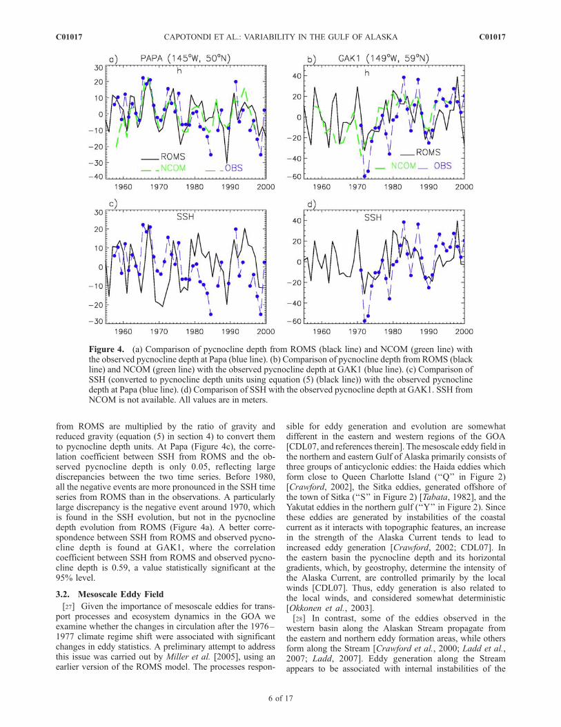
from ROMS are multiplied by the ratio of gravity andreduced gravity (equation (5) in section 4) to convert themto pycnocline depth units. At Papa (Figure 4c), the corre-lation coefficient between SSH from ROMS and the ob-served pycnocline depth is only 0.05, reflecting largediscrepancies between the two time series. Before 1980,all the negative events are more pronounced in the SSH timeseries from ROMS than in the observations. A particularlylarge discrepancy is the negative event around 1970, whichis found in the SSH evolution, but not in the pycnoclinedepth evolution from ROMS (Figure 4a). A better corre-spondence between SSH from ROMS and observed pycno-cline depth is found at GAK1, where the correlationcoefficient between SSH from ROMS and observed pycno-cline depth is 0.59, a value statistically significant at the95% level.

3.2. Mesoscale Eddy Field

[27] Given the importance of mesoscale eddies for trans-port processes and ecosystem dynamics in the GOA weexamine whether the changes in circulation after the 1976–1977 climate regime shift were associated with significantchanges in eddy statistics. A preliminary attempt to addressthis issue was carried out by Miller et al. [2005], using anearlier version of the ROMS model. The processes respon-

sible for eddy generation and evolution are somewhatdifferent in the eastern and western regions of the GOA[CDL07, and references therein]. Themesoscale eddy field inthe northern and eastern Gulf of Alaska primarily consists ofthree groups of anticyclonic eddies: the Haida eddies whichform close to Queen Charlotte Island (‘‘Q’’ in Figure 2)[Crawford, 2002], the Sitka eddies, generated offshore ofthe town of Sitka (‘‘S’’ in Figure 2) [Tabata, 1982], and theYakutat eddies in the northern gulf (‘‘Y’’ in Figure 2). Sincethese eddies are generated by instabilities of the coastalcurrent as it interacts with topographic features, an increasein the strength of the Alaska Current tends to lead toincreased eddy generation [Crawford, 2002; CDL07]. Inthe eastern basin the pycnocline depth and its horizontalgradients, which, by geostrophy, determine the intensity ofthe Alaska Current, are controlled primarily by the localwinds [CDL07]. Thus, eddy generation is also related tothe local winds, and considered somewhat deterministic[Okkonen et al., 2003].[28] In contrast, some of the eddies observed in the

western basin along the Alaskan Stream propagate fromthe eastern and northern eddy formation areas, while othersform along the Stream [Crawford et al., 2000; Ladd et al.,2007; Ladd, 2007]. Eddy generation along the Streamappears to be associated with internal instabilities of the

Figure 4. (a) Comparison of pycnocline depth from ROMS (black line) and NCOM (green line) withthe observed pycnocline depth at Papa (blue line). (b) Comparison of pycnocline depth from ROMS (blackline) and NCOM (green line) with the observed pycnocline depth at GAK1 (blue line). (c) Comparison ofSSH (converted to pycnocline depth units using equation (5) (black line)) with the observed pycnoclinedepth at Papa (blue line). (d) Comparison of SSH with the observed pycnocline depth at GAK1. SSH fromNCOM is not available. All values are in meters.


6 of 17

C01017

flow, so that these eddies cannot directly be related to thelocal wind forcing [Okkonen et al., 2001]. Eddies propa-gating into the western basin along the margin of the GOAwill have a lagged correlation with the winds in theformation areas.[29] CDL07 has examined the relationship between eddy

variance and wind forcing by comparing the same ROMSsimulation analyzed here with a simulation forced bymonthly climatological fields. On interannual timescales,the forced simulation yields larger eddy variance in theeastern basin, while the variance in the western basin doesnot show significant differences between the two runs.Moreover, when the three model ensemble members areconsidered, it is found that the evolution of SSH anomaliesis very similar among ensemble members in the Haida andSitka eddy formation sites, while a large spread is found inthe evolution of SSH along the Alaskan Stream, suggestinga dominance of internal versus forced variations in thewestern basin in the model [CDL07].[30] The issue that we address here is whether a relation-

ship can be found between eddy variance and intensity ofthe gyre circulation. Differences of standard deviations ofSSH and pycnocline depth (Figure 5) between the periodafter the shift and the period before the shift show largervalues after 1977 in both the eastern and western margins.The larger standard deviation differences along the coast aremuch more evident in the SSH than in the pycnocline depthfield, for our choice of P1 and P2. In the eastern basin,localized maxima are found offshore of Queen CharlotteIsland (53�N, 130�W), where the Haida eddies are formed,while offshore of Sitka (57�N, 135�W) small areas of bothincreased and decreased variance are found. Enhancedvariance is also detected around the apex of the gulf, wherethe Yakutat eddies are generated. Away from the coastalregion, a broad band of increased variance is found between155�W and 135�W, south of �48�N. This area is notassociated with large mean variance (not shown). Theincreased variability in both SST and pycnocline depth afterthe climate shift in this region may be associated withincreased variance in the wind forcing.[31] To further quantify the relationship between eddy

statistics and gyre circulation, we examine the evolution of

eddy kinetic energy (EKE) in the ROMS simulation. To placethe pattern of EKE in the context of the gyre circulation, westart by computing the surface total kinetic energy (TKE):

TKE ¼ 0:5� u2 þ v2� �

; ð1Þ

where u and v are the total surface velocities from theROMS simulations, available at a monthly time resolution.The time mean TKE, averaged over the total duration ofthe integration (Figure 6a) maximizes in the area of theAlaskan Stream in the western GOA, but values larger than100 cm2 s�2 are also found on the eastern and northernpart of the basin, offshore of Queen Charlotte Island, andfrom Sitka to the apex of the gulf following the coast. TheEKE is computed using equation (1) after removing thelong-term mean from the velocities. The pattern of meanEKE (Figure 6b) also shows localized maxima in the area ofQueen Charlotte Island and Sitka, where the Haida and Sitkaeddies are formed, with maximum values of �80 cm2 s�2,and a broad area of values larger than 60 cm2 s�2 to thesouthwest of the core of maximum TKE. To assess thedegree of realism of the EKE pattern from ROMS, wecompute EKE from the AVISO altimeter data on the basisof monthly averaged SSH anomalies (long-term meanremoved):

EKEAVISO ¼ 0:5� u02g þ v02g

� �; ð2Þ

where u0g and v0g are the geostrophic velocities estimatedfrom the AVISO SSH:

u0g ¼ � g

f

Dh0

Dy; v0g ¼

g

f

Dh0

Dx; ð3Þ

with g being the acceleration of gravity, and f denoting theCoriolis parameter. The pattern of EKE from AVISO,relative to the period 1993–2004 (Figure 6c) is very similarto that computed by Ladd [2007] from weekly sea levelanomalies (SLA), but the maximum values in Figure 6c aresmaller than those in the paper by Ladd [2007] because ofthe monthly averaging. Comparison of Figures 6b and 6c

Figure 5. Changes in standard deviation of (a) SSH (cm) and (b) pycnocline depth (m) associated withthe 1976–1977 climate shift. The changes were computed as the differences between P2 (1977–1997)and P1 (1958–1975).


7 of 17

C01017

shows several discrepancies between the modeled andobservation-derived EKE patterns. The maximum EKEextending from Sitka to the west of the apex of the gulf,where the Yakutat eddies are formed is missing in themodel, suggesting that the generation of Yakutat eddies, aswell as the westward propagation of the eastern eddiesalong the coast [Crawford et al., 2000; Ladd, 2007] are notcorrectly captured by the model. The large values of EKEin the western margin of the GOA are confined within amuch narrower band in the map from the altimeter than inthe model. The values of EKE in the model are alsogenerally lower than those estimated from the altimetricobservations, a result likely due to the eddy-permitting (andnot fully resolving) nature of this ROMS simulation.[32] The changes in EKE associated with the 1976–1977

climate shift, estimated from ROMS as the difference be-tween P2 and P1 (Figure 6d) have a noisy structure, showingan overall increase in EKE along the coast after the shift, withsome localized areas where the EKE decreased after 1977.Since the western GOA eddies seem to originate primarilyfrom internal instability of the Alaskan Stream in the model,we compute an EKE index by averaging the EKE over thearea where the TKE is larger than 100 cm2 s�2 in the westernbasin (between 165�Wand 148�W, and north of 52�N). After

removing the monthly means and smoothing the EKE timeseries with a three-point binomial filter, we compare theevolution of the EKE index with both the PDO and NPGOindices (Figure 7).[33] The correlation coefficient between EKE in the

western basin and the PDO is 0.54, which is statisticallysignificant at the 99% level. The correlation with the NPGOindex, on the other hand, is only 0.22, whose statisticalsignificance is below the 90% level. CDL07 has shown thatthe PDO index was statistically significant correlated withthe Principal Component (PC) of the leading EmpiricalOrthogonal Function (EOF) of SSH from the same modelsimulation, a mode of variability corresponding to varia-tions in the gyre strength. Thus, although unrelated with thelocal wind forcing, eddy activity in the western GOAincreases with increasing gyre circulation strength. Thestatistically significant correlation between EKE in thewestern basin and PDO index is consistent with the largecoherent loading of the PDO mode along the coast. Whilethe correspondence between eddy production and circulationstrength is relatively well established in the eastern andnorthern basin [Crawford, 2002; CDL07; Ladd, 2007], muchless is known for the western eddies. Here we show thatwestern eddies are also related to some large-scale mode of

Figure 6. (a) Mean surface total kinetic energy in ROMS over the total duration of the integration(1950–2004). Contour interval is 100 cm2 s�2. Values larger than 100 cm2 s�2 are shaded. (b) Meansurface eddy kinetic energy (EKE) in ROMS (1950–2004). Contour interval is 20 cm2 s�2, and valueslarger than 20 cm2 s�2 are shaded. (c) EKE from AVISO (1993–2004) based on monthly averages ofSSH anomalies. Contour interval is 20 cm2 s�2, and values larger than 20 cm2 s�2 are shaded. (d) EKEdifference between P2 (1977–1997) and P1 (1958–1975). Contour interval is 10 cm2 s�2. Orange shadingindicates positive values, while blue shading is for negative values.


8 of 17

C01017

climate variability and the associated circulation variations.This suggests that if climatemodels can successfully simulatethe major modes of climate variability and the associatedchanges in the large-scale ocean circulation, eddy statisticscould be partially inferred from those circulation changes.

4. Ekman Versus Rossby Wave Dynamics

[34] To elucidate the dynamical processes involved in theocean adjustment to varying wind forcing we use theEkman pumping and Rossby wave models considered byCADM05 and Qiu [2002]. These models have proved veryuseful in accounting for a large fraction of pycnocline depthand SSH variability at interannual and longer timescalesin the northeast Pacific [Lagerloef, 1995; Cummins andLagerloef, 2002, 2004], but the relative role of local Ekmanpumping forcing versus westward Rossby wave propagationis not entirely clear.[35] The Ekman pumping model:

dh

dt¼ �WE � lh; ð4Þ

relates the time rate of change of the pycnocline depth h tothe Ekman pumping WE in the presence of dissipation, asdescribed by a linear damping term with coefficient l. Asimilar equation can be derived for SSH using a two-layer

approximation for the ocean [Qiu, 2002]. Assuming that thebottom layer is much deeper than the top layer, the SSH (z)is related to the pycnocline depth:

V ¼ g0=gð Þh; ð5Þ

where g0 is the reduced gravity, g0 = (r2 � r1)g/ro, with r1and r2 the densities of the top and bottom layers,respectively, and ro is the mean density of seawater. TheEkman pumping is the vertical velocity at the base of theEkman layer due to the divergence of the Ekman currents,and is defined as the vertical component of the curl of thewind stress t divided by the Coriolis parameter f and themean density of seawater ro:

WE ¼ r� trof

� �� : ð6Þ

[36] Monthly values of WE from the NCEP-NCAR rean-alyses, the same forcing that drives the ROMS simulation,are used to force (4). Equation (4) is solved using a second-order accurate trapezoidal scheme as:

hnþ1 ¼ a1hn þ a2W

nþ1=2E ; ð7Þ

where a1 = (2 � lDt)/(2 + lDt), a2 = (2Dt)/(2 + lDt),and WE

n+1/2 is the average Ekman pumping at times nand n + 1. The initial condition for (4) is the pycnoclinedepth (or SSH) at the initial time (January 1950). The valueof l at each grid point has been defined as in the paper byCADM05 as the value that maximizes the correlationbetween pycnocline depth (or SSH) from the simple model(4) and that from ROMS. The maximum correlations (asfunction of l) are shown in Figure 8 for both pycnoclinedepth (Figure 8a) and SSH (Figure 8c).[37] The correlation pattern is very similar to that com-

puted by CADM05 (their Figure 6b) with the largest valuesin the center of the gulf and very low correlations in a bandalong the western margin. As seen in section 3, the Ekmanpumping anomalies associated with the 1976–1977 climateshift are upwelling favorable southwest of Kodiak Islandand the Alaska Peninsula (Figure 2), while the pycnocline isdeeper after the shift in that area (Figure 1). The spatialstructure of Ekman pumping variations associated with theregime shift in the mid-1970s is similar to the leading EOFof interannual Ekman pumping anomalies [Cummins andLagerloef, 2002]. Pycnocline depth variations along thewestern side of the Gulf of Alaska are not forced by thelocal Ekman pumping, thus explaining the low correlationsin Figure 8 in that area.[38] The correlation patterns in Figures 8a and 8c although

broadly similar to that computed by CADM05, shows moresmall-scale features than the corresponding pattern ofCADM05 because of the eddy-permitting nature of ROMS.ROMS correlations are also generally lower than thosecomputed using NCOM, especially the SSH correlations(Figure 8c). Notice the coastal area of relatively largecorrelations from north of Queen Charlotte Island to theapex of the gulf in both Figures 8a and 8c. That is an area

Figure 7. Comparison of the EKE in the western GOA(dot-dashed line) with (a) the PDO and (b) the NPGO indices(solid lines). The EKE index is computed by averagingthe EKE over the area where the mean EKE is larger than100 cm2 s�2 between 148�Wand 165�Wand north of 52�N.This mainly captures EKE variations along the AlaskanStream. The correlation coefficient between EKE and PDOindex is 0.54 when the PDO leads the EKE by 1month, whilethe correlation coefficient with the NPGO is only 0.22.


9 of 17

C01017

where the anomalous Ekman pumping associated with the1976–1977 climate shift is downwelling favorable, and hasa center of action centered around 140�W, 56�N (Figure 2).[39] Figures 8b and 8d show the values of l�1 that

maximize the correlation between the evolution of theh (Figure 8b) and SSH (Figure 8d) fields in ROMS andthe corresponding fields from the Ekman pumping model.Values are shown only over the areas where the correlationsare larger than 0.5. Despite the noisy spatial pattern of l�1,in the central GOA, where correlations are larger, l�1 is�10–20 months, in agreement with the findings ofCADM05, as well as the value of 17 months found byCummins and Lagerloef [2002] at Papa, using statisticalmethods.[40] Qiu [2002] has shown that the temporal evolution of

SSH anomalies from TOPEX/Poseidon altimetry (October1992 to July 2000) was well described by a dynamical frame-work that included westward propagation of the anomaliesat the speed of first-mode baroclinic Rossby waves. Themodel for the evolution of pycnocline depth in the presenceof Rossby wave propagation hR can be written as:

@hR@t

þ cR@hR@x

¼ �WE � l1hR; ð8Þ

where cR =�bR2 is the phase speed of long baroclinic Rossbywaves, a function of the Rossby radius of deformation R, andthe latitudinal gradient of the Coriolis parameter b. l1 is aRayleigh friction coefficient, which, following CADM05 hasbeen chosen to be (4 years)�1. The Rossby wave phase speedis latitude dependent, decreasing with increasing latitude, andis also influenced by the background mean flow [Killworth etal., 1997]. Following Killworth et al. [1997], we have chosencR � 0.8 cm s�1 along 50�N. Equation (8) can be solved byintegrating along Rossby wave characteristics in the x-t plane:

hR x; tð Þ ¼ hR xE; t � tEð Þe�l1tE þZ x

xE

WE x; t � tx� �cR xð Þ e�l1 txdx:

ð9Þ

[41] The solution at point x and time t is the superpositionof two terms: the first term on the rhs of (9) is thecontribution of disturbances originating at the easternboundary xE and reaching point x at time t with a transittime tE =

R x

xEdx/cR(x); the second term on the rhs of (9) is

the contribution of the anomalies excited by the Ekmanpumping east of the target point x, with tx =

R x

x ds/cR(s)being the transit time from point x to point x. Both boundaryand wind-forced terms decay while propagating westwardwith an e-folding time (1/l1). A similar equation holds for

Figure 8. (a) Maximum correlation, as a function of l, between the pycnocline depth computed usingthe local Ekman pumping model and the pycnocline depth from ROMS. Contour interval is 0.1. Valueslarger than 0.5 are shaded. (b) Values of l�1 (in months) yielding the correlations in Figure 8a. Values areshown only over the areas where correlations in Figure 8a are larger than 0.5. Contour interval is 4 monthsfor values lower than 20 months and 20 months for values larger than 20 months. (c) Same as in Figure 8a,but for SSH. (d) Same as in Figure 8b, but for SSH.


10 of 17

C01017

the SSH with the relationship between SSH and pycnoclinedepth given by (5).[42] In Figure 9, the evolution of pycnocline depth and

SSH along 50�N are compared with the evolution of SSHanomalies from the AVISO data set over the period 1993–2004 (satellite data start in 1993). The evolution of SSHanomalies obtained using the Ekman pumping model (4)and the Rossby wave model (8) over the same period arealso shown for comparison. Pycnocline depth values areconverted to SSH units using (5), so that all the fields can beplotted in the same units (cm) and with a similar contourinterval.[43] The SSH anomalies from the altimeter (Figure 9c)

show a clear indication of westward propagation at a speedvery similar to the 0.8 cm s�1 used for the Rossby wavemodel (Figure 9e), as seen from the comparable slope of thephase lines. Similar propagating characteristics are seen inthe SSH field from ROMS, whose Hovmoller diagramcompares remarkably well with that from the AVISO data,given the presence of internal variability that may differ inthe model and observations. Pycnocline depth anomalies,on the other hand, have a more stationary evolution, which

has a good resemblance with that obtained from the Ekmanpumping model (Figure 9d). A close inspection of Figures 9aand 9b reveals that anomalies generated around 140�W havea much weaker signature in the pycnocline depth field versusthe SSH field in the center of the basin (145�W–165�W),so that westward propagation is much less obvious in thepycnocline depth field. These conclusions derived fromvisual inspection can be quantified using correlation anal-ysis. In Figure 10, the evolution of the SSHs from AVISOand ROMS at each longitude, as well as the evolution ofpycnocline depth from ROMS are correlated with the timeseries generated using both the Ekman and Rossby modelsalong 50�N over the period 1993–2004. In the longituderange 143�W–163�W correlations between the SSHs fromboth ROMS and AVISO and those derived from the Ekmanpumping model drop to values very close to zero (and evenbelow zero for AVISO), and are much lower than thecorrelations with the SSHs obtained from the Rossbymodel, which tend to remain above 0.5. On the other hand,pycnocline depth from ROMS tends to be described com-parably well by both simple models, as the correlations aremuch more similar across the basin, except for the 155�W–

Figure 9. (a) Hovmoller diagram of pycnocline depth from ROMS along 50�N. Pycnocline depth hasbeen converted to SSH units using equation (5). (b) Hovmoller diagram of SSH from ROMS along 50�N.(c) Same as in Figure 9b, but for SSH from the AVISO archive. (d) Evolution of SSH along 50�Nobtained using the Ekman pumping model. (e) SSH along 50�N from the Rossby wave model. Contourinterval is 2 cm.


11 of 17

C01017

160�W and 171�W–178�W longitude bands, and east of134�W, where the correlations with the Ekman pumpingmodel drop to values lower than 0.3.[44] Along 50�N the evolution of SSH from ROMS is

similar to that derived from altimeter observations, and theevolution of both modeled and observed SSHs clearly showwestward Rossby wave propagation. Is similar agreementfound at different latitudes? As an example, we show inFigure 11 Hovmoller diagrams of pycnocline depth, SSHfrom ROMS and SSH from AVISO along 53�N. Along thislatitude westward propagation is much less pronounced inall three fields, and is not observed all across the basin as at50�N. In the AVISO data (Figure 11c) westward propagatingfeatures can be observed east of 140�W, and west of 155�W.This westward propagation close to the margins of the GOAmay be associated with the propagation of eddies along thecoast. In the model’s fields (Figures 11a and 11b) westwardpropagation is less evident. As noted for the evolution along50�N, the correspondence between pycnocline depth anoma-lies and SSH anomalies in ROMS varies as a function oflongitude, and large SSH signals, like the one centered around155�W from 1993 to 2000 seem to have a much weakerpycnocline depth signature.

[45] To further examine the relationship between pycno-cline depth and SSH we show, in Figure 12, the spatialdistribution of the correlation between the two fields.Correlations are larger than 0.7 over a broad area, but dropto values below 0.7 in the center of the gyre. The averagecorrelation between the two fields in the region 155�W–145�W, 52�N–54�N (dot-dashed box in Figure 12) is �0.6.Why is the SSH-pycnocline depth correspondence lower inthe center of the gyre? Since the pycnocline is shallower inthis region, one may think that the evolution of pycnoclinedepth is affected by mixed layer processes and not onlyconsists of dynamical signals excited by the varying windforcing. In Figure 13 we compare the evolution of pycno-cline depth and SSH averaged in the box 155�W–145�W,52�N–54�N. The largest discrepancies between the twotime series are observed from 1960 to 1974, when SSHvariations are much weaker, and sometimes of opposite sign,than pycnocline depth changes, and after 1990, when SSHanomalies are larger than pycnocline depth anomalies.[46] To elucidate the relationship between the evolution

of SSH and pycnocline depth with the surface forcing, thetime series of the Ekman pumping averaged over the samebox is also shown in Figure 13. The correlation betweenpycnocline depth and Ekman pumping is 0.7, with the Ekman

Figure 10. (a) Correlation between AVISO SSH with the SSH from the Ekman pumping model (solidline) and the Rossby wave model (dot-dashed line) along 50�N and over the period 1993–2004. (b) Sameas in Figure 10a, but for ROMS SSH. (c) Same as in Figure 10a, but for ROMS pycnocline depth.


12 of 17

C01017

pumping leading by 4 months, while the correlation betweenSSH andWE is only 0.36 when the Ekman pumping leads by5 months. Notice, in particular, that the evolution of pycno-cline depth from 1960 to 1974 tracks very closely theevolution of WE during the same period, while the evolutionof SSH does not. Thus, pycnocline depth changes appear tobe more directly controlled by the Ekman pumping forcingthan SSH in the center of the Alaska Gyre. The SSHevolution may also be influenced by diabatic processes,while pycnocline depth, being further away from the surface,may primarily capture the dynamical signals associated withvarying wind forcing. We plan to use sensitivity experimentswhere either anomalous wind forcing or anomalous buoyancyforcing is prescribed to clarify this point in a future study.[47] Are the SSH and pycnocline depth variations in the

center of the Alaska gyre related to the PDO and NPGO?Figures 14a and 14b show the comparison between the timeseries of pycnocline depth and SSH, averaged over the boxin Figure 12, with the NPGO index. Notice that the NPGOindex is shown with sign reversed for ease of comparison.Positive NPGO corresponds to an intensification of theeastern limbs of both subtropical and subpolar gyres, andis associated with negative SSH and pycnocline depthanomalies in the GOA.

[48] The correlation coefficient between pycnocline depthand NPGO is 0.69 when the NPGO index leads by onemonth. This correlation is statistically significant at the 95%level. The correlation coefficient between SSH variationsand NPGO index is 0.54 when the NPGO leads SSH bytwo months, which is marginally significant at the 95% level.The comparison of both pycnocline depth and SSH timeseries with the PDO index (Figures 14c and 14d, respec-tively) shows a lower degree of agreement. Pycnocline depthvariations are practically uncorrelated with the PDO index(correlation coefficient is 0.09), while SSH has a correla-tion coefficient of 0.39 (PDO leading by 7 months), whichis only marginally significant at the 90% level. The box wehave chosen lays in the area of positive SSH anomalies ofthe PDO pattern, but is very close to the nodal line of thatpattern. The lower agreement may be partly due to theposition of the box relative to the spatial structure of thePDO mode. Di Lorenzo et al. [2008] have emphasizedthe large correlation between NPGO and coastal upwelling.Here we find that open ocean upwelling, as described bychanges in pycnocline depth, is also related to the NPGO (butnot the PDO).[49] Thus, the evolution of both pycnocline depth and

SSH can be related to one of the leading North Pacificmodes of climate variability. However, pycnocline depth is

Figure 11. Hovmoller diagram of (a) pycnocline depth, (b) SSH from ROMS, and (c) SSH from AVISOalong 53�N. Pycnocline depth has been converted to SSH units using equation (5). Contour interval is2 cm. Blue shading is for negative values (shallower pycnocline, negative SSHs), while orange shadingis for positive values (deeper pycnocline, positive SSH anomalies).


13 of 17

C01017

more directly correlated to local wind forcing, and appears tobe the quantity that more clearly captures dynamical changesrelated to the NPGO mode of variability. This was not thecase for the EKE along the western margin of the GOA,which was correlated with the PDO, but not the NPGO.

5. Summary and Conclusions

[50] In this paper we have used an eddy-permitting oceanmodel of the northeast Pacific to examine the role of eddies

in the adjustment of the Gulf of Alaska circulation tochanges in the surface wind forcing. We have also com-pared the dynamical information contained in the evolutionof the sea surface height (SSH) field with that of pycnoclinedepth. Results from the eddy-permitting model are inagreement with the findings of a previous study whichwas based on a relatively coarse-resolution global oceanmodel [CADM05] in that local Ekman pumping can explaina large fraction of both pycnocline and SSH variability in

Figure 12. Instantaneous correlations between pycnocline depth and SSH in ROMS. Contour interval is0.1. Values larger than 0.7 are shaded. The dot-dashed box shows the area where averaged time series ofthe two fields are computed and compared.

Figure 13. Comparison between the time series of pycnocline depth (black line), SSH (blue line), andEkman pumping (red line) averaged over the box shown in Figure 12. All time series are normalized bytheir standard deviations. Notice that the Ekman pumping WE is shown with sign reversed for ease ofcomparison. The correlation coefficient between pycnocline depth and Ekman pumping is 0.70 when theEkman pumping leads by 4 months, while the correlation coefficient of SSH and WE is 0.36 when WE

leads by 5 months.


14 of 17

C01017

the center of the Gulf of Alaska (GOA), and in part of theeastern and northern coastal regions.[51] Pycnocline depth and SSH changes associated with

the 1976–1977 climate shift are qualitatively similar to thepattern of pycnocline depth changes computed by CADM05:the pycnocline shoals in the center of the gyre and deepensalong the coast, while the SSH field is higher along the coast,and lower in the interior after the shift. Because of theincreased zonal gradients of pycnocline depth, the circulationis stronger after the climate shift. The standard deviation ofSSH, as well as eddy kinetic energy (EKE), two measuresof the intensity of the mesoscale eddy field, are also generallylarger after the climate shift along the coastal areas.[52] SSH is usually considered the mirror image of

pycnocline depth (scaled by the ratio of reduced gravityand gravity), and containing the same dynamical informa-tion. The comparison of SSH and pycnocline depth evolutionreveals, however, subtle differences. At some latitudes,westward propagation is much clearer in the SSH field thanin the pycnocline depth field, and the relationship with thesurface forcing is not always the same. In the center of theAlaska gyre, the evolution of pycnocline depth is largelycorrelated with the local Ekman pumping, while the correla-tion between SSH and Ekman pumping is lower.

[53] The local forcing is, in turn, part of large-scalepatterns of atmospheric variability. The leading modes ofSSH variability over the northeast Pacific, as defined by DiLorenzo et al. [2008] include the Pacific Decadal Oscillation(PDO) and the North Pacific Gyre Oscillation (NPGO).Pycnocline depth variations in the central Gulf of Alaskaare significantly correlated with the NPGO, while the rela-tionship between SSH and NPGO is more tenuous. The windstress pattern associated with the positive phase of the NPGO[Di Lorenzo et al., 2008, Figure 3b] shows positive zonalwind stress anomalies centered at approximately 45�N,which can be expected to be associated with positive(upwelling favorable) WE anomalies around 50�N–55�N.Pycnocline depth variations in that area are significantlycorrelated with WE variations, which may be primarilyassociated with the NPGO mode of variability. Di Lorenzoet al. [2008] have stressed the connection between NPGOand coastal upwelling along the California current. Ourresults seem to indicate that this relationship also holds inthe center of the GOA, where pycnocline depth changesare indicative of variations in open ocean upwelling.[54] The mesoscale eddy field in the Gulf of Alaska plays

a fundamental role in the transport of iron and nutrientsbetween the coastal regions and the open ocean, and eddy

Figure 14. (a) Comparison of pycnocline depth (black line) from ROMS in the box shown in Figure 12with the NPGO index (red line). The NPGO index is shown with sign reversed for ease of comparison.The correlation coefficient between the two time series is 0.67 when the NPGO index leads by onemonth. (b) Same as in Figure 14a, but for SSH (blue line). The correlation coefficient between the twotime series is 0.53 when the NPGO leads by two months. (c) Comparison of pycnocline depth fromROMS in the box shown in Figure 12 with the PDO index (green line). The correlation coefficient is only0.08. (d) Same as Figure 14c, but for SSH. The correlation coefficient between SSH and PDO is 0.35when the PDO leads by 9 months. All time series have been normalized by their standard deviations andsmoothed with a three-point binomial filter.


15 of 17

C01017

statistics is considered very important for biological pro-cesses. A major issue concerns the possible changes in eddystatistics that may occur because of global warming. Thecurrent generation of climate models used for climatechange projections is run at a horizontal resolution that isunable to capture mesoscale eddies, so that informationabout eddy statistics changes will not be readily available.[55] Previous studies have shown that the eddy field in

the eastern basin is related to the local wind forcing, so thatdownwelling favorable winds lead to a stronger Alaskacurrent and a more energetic eddy field. Eddies in the westernbasin are generated by internal instabilities of the flow, ordrifted from the eastern and northern formation sites, so thatthey are not expected to be related to the local wind forcing.In this study we have examined the relationship between theeddy kinetic energy (EKE) in the western basin and theleading modes of SSH variability. A statistically significantcorrelation is found between EKE and the PDO, the mode ofvariability that seems to capture variations in the circulationstrength. Thus, if climate models can realistically simulatethe leading modes of climate variability in the northeastPacific and their evolution in future climate scenarios,possible changes in some aspects of eddy statistics may beinferred from the large-scale climate changes.

[56] Acknowledgments. We thank Patrick Cummins for providingthe time series of winter pycnocline depth at Ocean Weather Station Papaand the GLOBEC program for the long-termmeasurements at station GAK1.The easy access to oceanic observations (e.g., GAK1 and AVISO) has beenvery valuable and greatly appreciated. This study was supported by theNational Science Foundation (OCE-0452743, OCE-0452692, OCE-0452654, and NSF GLOBEC OCE-0606575). We thank the two anonymousreviewers for their excellent and constructive comments and suggestions.

ReferencesBond, N. A., J. E. Overland, M. Spillane, and P. Stabeno (2003), Recentshifts in the state of the North Pacific, Geophys. Res. Lett., 30(23), 2183,doi:10.1029/2003GL018597.

Capotondi, A., M. A. Alexander, C. Deser, and A. J. Miller (2005), Low-frequency pycnocline variability in the northeast Pacific, J. Phys. Oceanogr.,35, 1403–1420, doi:10.1175/JPO2757.1.

Chelton, D. B., and R. E. Davis (1982), Monthly mean sea-level variabilityalong the west coast of North America, J. Phys. Oceanogr., 12, 757–784,doi:10.1175/1520-0485(1982)012<0757:MMSLVA>2.0.CO;2.

Chelton, D. B., R. A. deSzoeke, and M. G. Schlax (1998), Geographicalvariability of the first baroclinic Rossby radius of deformation, J. Phys.Oceanogr. , 28 , 433 – 460, doi:10.1175/1520-0485(1998)028<0433:GVOTFB>2.0.CO;2.

Chhak, K. C., E. Di Lorenzo, P. Cummins, and N. Schneider (2008), Forc-ing of low-frequency ocean variability in the northeast Pacific, J. Clim.,doi:10.1175/2008JCLI2639.1, in press.

Combes, V., and E. Di Lorenzo (2007), Intrinsic and forced interannualvariability of the Gulf of Alaska mesoscale circulation, Prog. Oceanogr.,75, 266–286, doi:10.1016/j.pocean.2007.08.011.

Crawford, W. R. (2002), Physical characteristics of Haida eddies,J. Oceanogr., 58, 703–713, doi:10.1023/A:1022898424333.

Crawford, W. R., J. Y. Cherniawsky, and M. G. G. Foreman (2000), Multi-year meanders and eddies in the Alaskan Stream as observed by TOPEX/Poseidon altimeter, Geophys. Res. Lett., 27, 1025–1028, doi:10.1029/1999GL002399.

Crawford, W. R., P. J. Brickley, T. D. Peterson, and A. C. Thomas (2005),Impact of Haida eddies on chlorophyll distribution in the eastern Gulf ofAlaska, Deep Sea Res., Part II, 52, 975–989.

Crawford, W. R., P. J. Brickley, and A. C. Thomas (2007), Mesoscaleeddies determine phytoplankton distribution in northern Gulf of Alaska,Prog. Oceanogr., 75, 287–303, doi:10.1016/j.pocean.2007.08.016.

Cummins, P. F., and G. S. E. Lagerloef (2002), Low-frequency pycnoclinedepth variability at Ocean Weather Station P in the northeast Pacific,J. Phys. Oceanogr., 32, 3207–3215, doi:10.1175/1520-0485(2002)032<3207:LFPDVA>2.0.CO;2.

Cummins, P. F., and G. S. E. Lagerloef (2004), Wind-driven interannualvariability over the northeast Pacific Ocean, Deep Sea Res., Part I, 51,2105–2121, doi:10.1016/j.dsr.2004.08.004.

Curchitser, E. N., D. B. Haidvogel, A. J. Hermann, E. L. Dobbins, T. M.Powell, and A. Kaplan (2005), Multi-scale modeling of the North PacificOcean: Assessment and analysis of simulated basin-scale variability(1996 – 2003), J. Geophys. Res. , 110 , C11021, doi:10.1029/2005JC002902.

Di Lorenzo, E., et al. (2008), North Pacific Gyre Oscillation links oceanclimate and ecosystem change, Geophys. Res. Lett., 35, L08607,doi:10.1029/2007GL032838.

Doney, S. C., S. Yeager, G. Danabasoglu, W. G. Large, and J. C. McWilliams(2003), Modeling global oceanic interannual variability (1958–1997),simulation design and model-data evaluation, Tech. Note NCAR/TN-452+STR, Natl. Cent. for Atmos. Res., Boulder, Colo.

Ducet, N., P. Y. Le Traon, and G. Reverdin (2000), Global high-resolutionmapping of ocean circulation from TOPEX/Poseidon and ERS-1 and -2,J. Geophys. Res., 105, 19,477–19,498, doi:10.1029/2000JC900063.

Emery, W. J., and K. Hamilton (1985), Atmospheric forcing of interannualvariability in the northeast Pacific Ocean, J. Geophys. Res., 90, 857–868,doi:10.1029/JC090iC01p00857.

Enfield, D. B., and J. S. Allen (1980), On the structure and dynamics ofmonthly mean sea level anomalies along the Pacific coast of North andSouth America, J. Phys. Oceanogr., 10, 557–578, doi:10.1175/1520-0485(1980)010<0557:OTSADO>2.0.CO;2.

Freeland, H. J., K. Denman, C. S. Wong, F. Whitney, and R. Jacques(1997), Evidence of change in the winter mixed layer in the northeastPacific Ocean, Deep Sea Res., Part I, 44, 2117–2129, doi:10.1016/S0967-0637(97)00083-6.

Haidvogel, D. B., H. G. Arangoa, K. Hedstroma, A. Beckmannb, P.Malanotte-Rizzolic, and A. F. Shchepetkin (2000), Model evaluation experimentsin the North Atlantic Basin: Simulations in nonlinear terrain-followingcoordinates, Dyn. Atmos. Oceans, 32, 239–281, doi:10.1016/S0377-0265(00)00049-X.

Kalnay, E., et al. (1996), The NCEP/NCAR 40-year Reanalysis Project,Bull. Am. Meteorol. Soc., 77, 437–471, doi:10.1175/1520-0477(1996)077<0437:TNYRP>2.0.CO;2.

Killworth, P. D., D. B. Chelton, and R. A. de Szoeke (1997), The speed ofobserved and theoretical long extratropical planetary waves, J. Phys.Oceanogr., 27, 1946–1966, doi:10.1175/1520-0485(1997)027<1946:TSOOAT>2.0.CO;2.

Ladd, C. (2007), Interannual variability of the Gulf of Alaska eddy field,Geophys. Res. Lett., 34, L11605, doi:10.1029/2007GL029478.

Ladd, C., P. Stabeno, and E. D. Cokelet (2005), A note on cross-shelfexchange in the northern Gulf of Alaska, Deep Sea Res., Part II, 52,667–679, doi:10.1016/j.dsr2.2004.12.022.

Ladd, C., C. W. Mordy, N. B. Kachel, and P. J. Stabeno (2007), NorthernGulf of Alaska eddies and associated anomalies, Deep Sea Res., Part I,54, 487–509, doi:10.1016/j.dsr.2007.01.006.

Lagerloef, G. S. E. (1995), Interdecadal variations in the Alaska gyre,J. Phys. Oceanogr., 25, 2242–2258, doi:10.1175/1520-0485(1995)025<2242:IVITAG>2.0.CO;2.

Large, W. G., and S. Pond (1982), Sensible and latent heat flux measure-ments over the ocean, J. Phys. Oceanogr., 12, 464–482, doi:10.1175/1520-0485(1982)012<0464:SALHFM>2.0.CO;2.

Large, W. G., G. Danabasoglu, and S. C. Doney (1997), Sensitivity tosurface forcing and boundary-layer mixing in a global ocean model:Annual mean climatology, J. Phys. Oceanogr., 27, 2418 – 2447,doi:10.1175/1520-0485(1997)027<2418:STSFAB>2.0.CO;2.

Large, W. G., J. C. McWilliams, P. R. Gent, and F. O. Bryan (2001),Equatorial circulation of a global ocean climate model with anisotropichorizontal viscosity, J. Phys. Oceanogr., 31, 518–536, doi:10.1175/1520-0485(2001)031<0518:ECOAGO>2.0.CO;2.

Le Traon, P. Y., and G. Dibarboure (1999), Mesoscale mapping capabilitiesof multi-satellite altimeter missions, J. Atmos. Oceanic Technol., 16,1208 – 1223, doi:10.1175/1520-0426(1999)016<1208:MMCOMS>2.0.CO;2.

Levitus, S., R. Burgett, and T. Boyer (1994),World Ocean Atlas 1994, vol. 4,Temperature, NOAA Atlas NESDIS, vol. 4, pp. 3–4, NOAA, SilverSpring, Md.

Mantua, N. J., S. Hare, Y. Zhang, J. M. Wallace, and R. Francis (1997), APacific interdecadal climate oscillationwith impacts on salmon production,Bull. Am. Meteorol. Soc., 78, 1069 – 1079, doi:10.1175/1520-0477(1997)078<1069:APICOW>2.0.CO;2.

Marchesiello, P., J. C. McWilliams, and A. Shchpetkin (2003), Equilibriumstructure and dynamics of the California Current System, J. Phys. Ocea-nogr., 33, 753–783, doi:10.1175/1520-0485(2003)33<753:ESADOT>2.0.CO;2.


16 of 17

C01017

Meyers, S. D., and S. Basu (1999), Eddies in the eastern Gulf of Alaskafrom TOPEX/POSEIDON altimetry, J. Geophys. Res., 104, 13,333–13,343, doi:10.1029/1999JC900039.

Miller, A. J., et al. (2005), Interdecadal changes in mesoscale eddy variancein the Gulf of Alaska circulation: Possible implications for the Steller sealion decline, Atmos. Ocean, 43, 231–240, doi:10.3137/ao.430303.

Nitta, T., and S. Yamada (1989), Recent warming of tropical SST and itsrelationship to the Northern Hemisphere circulation, J. Meteorol. Soc.Jpn., 67, 375–383.

Okkonen, S. R., G. A. Jacobs, E. J. Metzger, H. E. Hurlburt, and J. F.Shriver (2001), Mesoscale variability in the boundary current of theAlaska Gyre, Cont. Shelf Res., 21, 1219–1236, doi:10.1016/S0278-4343(00)00085-6.

Okkonen, S. R., T. J. Weingartner, S. L. Danielson, D. L. Musgrave, andG. M. Schmidt (2003), Satellite and hydrographic observations of eddy-induced shelf-slope exchange in the northwestern Gulf of Alaska,J. Geophys. Res., 108(C2), 3033, doi:10.1029/2002JC001342.

Qiu, B. (2002), Large-scale variability in the midlatitude subtropical andsubpolar North Pacific Ocean: Observations and causes, J. Phys. Oceanogr.,32, 353 – 375, doi:10.1175/1520-0485(2002)032<0353:LSVITM>2.0.CO;2.

Shchepetkin, A. F., and J. C. McWilliams (2005), The regional oceanicmodeling system (ROMS): A split-explicit, free-surface, topography-following coordinate oceanic model, Ocean Modell., 9, 347–404,doi:10.1016/j.ocemod.2004.08.002.

Smith, T. M., and R. W. Reynolds (2004), Improved extended reconstruc-tion of SST (1854–1997), J. Clim., 17, 2466–2477, doi:10.1175/1520-0442(2004)017<2466:IEROS>2.0.CO;2.

Spencer, R. W. (1993), Global oceanic precipitation from the MSU during1979–91 and comparison to other climatologies, J. Clim., 6, 1301–1326,doi:10.1175/1520-0442(1993)006<1301:GOPFTM>2.0.CO;2.

Tabata, S. (1982), The anticyclonic, baroclinic eddy off Sitka, Alaska, in thenortheast Pacific Ocean, J. Phys. Oceanogr., 12, 1260 – 1282,doi:10.1175/1520-0485(1982)012<1260:TABEOS>2.0.CO;2.

Trenberth, K. E., and J. W. Hurrell (1994), Decadal atmosphere-oceanvariations in the Pacific, Clim. Dyn., 9, 303 – 319, doi:10.1007/BF00204745.

Xie, P., and P. A. Arkin (1996), Analyses of global monthly precipitationusing gauge observations, satellite estimates, and numerical model pre-dictions, J. Clim., 9, 840 – 858, doi:10.1175/1520-0442(1996)009<0840:AOGMPU>2.0.CO;2.

Yasuda, T., and K. Hanawa (1997), Decadal changes in mode waters in themidlatitude North Pacific, J. Phys. Oceanogr., 27, 858–870, doi:10.1175/1520-0485(1997)027<0858:DCITMW>2.0.CO;2.

��M. A. Alexander and A. Capotondi, PSD, ESRL, NOAA, 325 Broadway,

Boulder, CO 80305, USA. ([email protected])V. Combes and E. Di Lorenzo, School of Earth and Atmospheric

Sciences, Georgia Institute of Technology, Atlanta, GA 30332, USA.A. J. Miller, Scripps Institute of Oceanography, 9500 Gilman Drive, La

Jolla, CA 93093, USA.


17 of 17

C01017

Documents

Low-frequency variability in the Gulf of Alaska from ...horizon.ucsd.edu/miller/download/GoA_variability/GoA_variability.pdf · Low-frequency variability in the Gulf of Alaska from