Risk in Water Resources Management (Proceedings of Symposium H03 held during IUGG2011 in Melbourne, Australia, July 2011) (IAHS Publ. 347, 2011).

Copyright © 2011 IAHS Press

77

Low-flow risk assessment for water management MIKHAIL BOLGOV1 & ELENA KOROBKINA2

1 Water Problems Institute, RAS, Gubkin St., Moscow 119333, Russia bolgovmv@mail.ru

2 Institute for Water and Environmental Problems, SB RAS, Morskoy Prosp., 2, Novosibirsk 630090, Russia Abstract Risk assessments related to increasing aridity of climate are important, particularly for stable operation of water systems and optimization of water resources management. For this purpose several approaches for regionalization and evaluation of parameters of long-term river flow fluctuations are considered and the method of simulation of synthetic time series of inflow to reservoirs is proposed. To validate the applicability of the Markov stochastic model to describe the of probability of cycling of dry and wet years, the characteristics of distribution of excursions below thresholds (duration and frequency of events) and the minima in the time series of fluvial discharge smoothed regarding N-years were calculated. This approach has been used for assessment of reliability of the complex water system in the Volga River basin under drought conditions and can be applied to evaluation of probability of long periods of low flows on the rivers in Siberia and in the Far East (Russian Federation). Key words river–runoff; low flow; stochastic modelling; parameters of distribution INTRODUCTION

The feature of long-term annual river–runoff time series to form groups of low-flow or high-flow years requires the streamflow control by reservoirs and the optimization of water resources manage-ment and development of operating rules to minimize negative consequences of runoff fluctuations. For the purpose of maintenance of sustained functioning of water resources systems during a low-flow period (including long duration), the method of simulation of synthetic time series of inflow to reservoir were applied to study water resources system in the Volga River basin and in some rivers of Siberia and the Far East. For simulating synthetic series, we need to have a clear idea about the stochastic model of runoff fluctuation which it is supposed to use and to get reliable estimation of parameters of this model on the basis of observed data. In this study the runoff series is generated based on the Markov stochastic model. In the first part of the study, the method of estimation of distribution parameters is discussed. This technique was applied to the river basins located in Siberia and the Far East. The second part of the study focused on the assessment of reliability of the complex water system in the Volga River basin under drought conditions. THE APPROACH OF SPATIAL GENERALIZATION OF THE HYDROLOGICAL PARAMETERS

Description of river–runoff fluctuation regularities using probability distribution functions is based on estimates of distribution parameters from the observed data. In most cases, the estimates of such parameters as coefficients of autocorrelation R(1) and asymmetry (skewness) Cs (or ratio Cs/Cv) from the time series of annual discharge cannot have reliable values due to the limitations of the runoff data available. To get more precise values of parameters R(1) and Cs/Cv we use the approach of spatial generalization of the parameters. Application of this method to study watersheds (gauging stations) to be spatial aggregated into some homogeneous groups makes it possible to generalize estimated parameters for the group of watersheds on the basis of aggregated time series for the component watersheds. This approach of joint analysis of hydrological time series was proposed by Kritskii & Menkel (1981) in the 1970s and then, following their methodology, was developed by Sotnikova (1988) and Bolgov et al. (1993). The dispersion of estimated parameters σ2 is caused by heterogeneity of sample data, which in turn is the result of two reasons. The first reason is fluctuations of runoff factors for the watersheds

Mikhail Bolgov & Elena Korobkina

78

and it can be explained by limitation of observing data for watersheds, i.e. random factor. The second reason connects with differences in climate and landscape of watersheds, i.e. with geographic features of the study area. The main idea of Kritskii & Menkel (1981) is that dispersion σ2 can be considered as a result of joint influence of these two reasons and thus can be divided to two components: random component 2

rσ and geographic component 2gσ of full dispersion:

222rg σσσ += (1)

Thus, the delineation of groups and corresponding spatial generalization of estimated parameters of flow probability distribution is based on the special technique of splitting the dispersion of estimated parameters σ2 (we will call it full dispersion) for two components in the following way. On the basis of any classification principles the study area is divided in some groups of watersheds. It can be made according to climate and landscape features or typical hydrological patterns of water bodies of the investigated area. For every group of watersheds the full dispersion and random component of dispersion of estimated parameters are determined using observed runoff data for component watersheds. Full dispersion of an estimated parameter for a group of watersheds is given by:

)1/()( 2

1

2 −−=∑=

nxx av

n

iiσ (2)

where n is the number of components of the group of watersheds (gauging stations), index i refers to the individual watershed of the group, xi is a sample estimate of parameters from observed time series for the ith watershed, xav is a mean value of estimated parameter for the group of watersheds. The random component of dispersion 2

rσ is determined by theoretical formulae as average dispersion of estimated parameter determined by limited sample:

∑=

=n

irr ni

1

22 /σσ (3)

where irσ is standard deviation for the ith individual watershed of the group. As an example, for

calculation of random component of dispersion of parameter Cs/Cv for every individual object of grouped watersheds, we used the formula proposed by Blokhinov (1974):

42)/( 242661

iii

i vviv

CvCsr CCnC

++=σ (4)

where index i refers to the ith individual watershed of the group, ni is the sample size, ivC the

coefficient of variation. Thus, the geographic component of dispersion 2

gσ is expressed from equation (1) as differences between full dispersion and random component:

222rg σσσ −= (5)

When the geographic component of dispersion does not exceed the random component, the group of watersheds can be considered as homogeneous and it is possible to add other next watersheds to “joint watershed” to calculate the value of spatially generalized parameter. Dispersion 2

avσ of parameter estimated by averaged data of all grouped time series in the aggregate

is determined by deviation of the true value of parameter for ith watershed ix−

related to average value of parameter for whole aggregated data xav, which can be rewritten as sum of deviations

)()()( iaviav xxxxxx−−−−

−+−=− , where −x is the true value of parameter for the ensemble of watersheds.

First deviation is calculated as dispersion for n random values of averaged parameter for all individual watersheds of study group, namely as nr /2σ , and the second component reflects the geographic heterogeneity of study area. Thus the dispersion of the generalized parameter is

Low-flow risk assessment for water management

79

calculated by the formula:

22

2g

rav n

σσσ += (6)

From equation (6) we can see that with increasing number of grouping watersheds the accuracy of calculation of the generalized parameter is also increased. But together with this, the grouping of a large number of watersheds means they are situated in different geographical zones with significantly varied conditions of runoff formation. This leads to heterogeneity of observed data, which in turn causes the rise of the geographical component of dispersion. Therefore, in our case the procedure of optimization of a number of objects composed of a group of watersheds is based on two conditions which need to be satisfied. The aggregation of separate watersheds into the “joint watershed” should proceed until the geographic component of dispersion does not exceed the random component and the dispersion of parameter estimated by the averaged data of generalized time series 2

avσ is minimized. If the first condition 22rg σσ ≤ is not

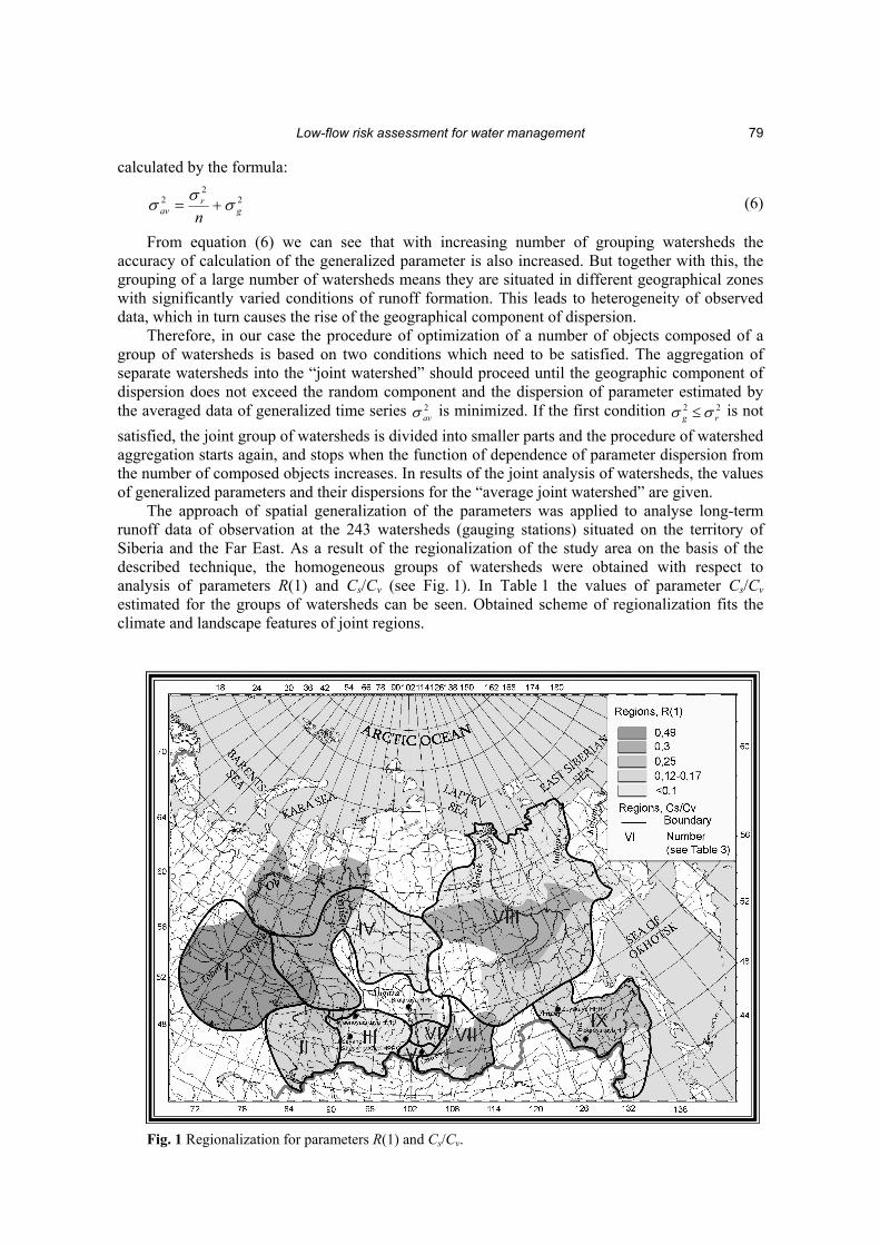
satisfied, the joint group of watersheds is divided into smaller parts and the procedure of watershed aggregation starts again, and stops when the function of dependence of parameter dispersion from the number of composed objects increases. In results of the joint analysis of watersheds, the values of generalized parameters and their dispersions for the “average joint watershed” are given. The approach of spatial generalization of the parameters was applied to analyse long-term runoff data of observation at the 243 watersheds (gauging stations) situated on the territory of Siberia and the Far East. As a result of the regionalization of the study area on the basis of the described technique, the homogeneous groups of watersheds were obtained with respect to analysis of parameters R(1) and Cs/Cv (see Fig. 1). In Table 1 the values of parameter Cs/Cv estimated for the groups of watersheds can be seen. Obtained scheme of regionalization fits the climate and landscape features of joint regions.

Fig. 1 Regionalization for parameters R(1) and Cs/Cv.

Mikhail Bolgov & Elena Korobkina

80

Table 1 Results of regionalization of Cs/Cv Region no. N Cs/Cv 2

avσ

I 38 1.993 0.027 II 43 1.894 0.040 III 24 1.764 0.115 IV 17 2.170 0.180 V 6 2.300 0.328 VI 5 1.791 0.126 VII 18 2.015 0.071 VIII 38 1.788 0.048 IX 23 1.741 0.061 n: the number of joined watersheds; Cs/Cv: mean value of parameter for the region; avσ : dispersion. ABOUT MARKOVIAN CHARACTER OF LONG-TERM RUNOFF FLUCTUATIONS

Characteristics of long-term river runoff fluctuations, such as the parameters of 1-D distributions and probabilities of multiyear droughts are determined by statistical analysis of the time series runoff. For this purpose the annual inflow for six water bodies in Siberia and in the Far East was examined. To validate the applicability of the Markov stochastic model to description of probability of cycling of dry and wet years, the characteristics of distribution of excursions below threshold levels (such as duration and frequency of events) and the minima in the time series of fluvial discharge smoothed regarding N years were calculated. Threshold levels are chosen as quantiles of 1-D distributions. Figure 2 shows the number (frequency) and the mean duration of excursions in the simulated and observed time series (for the period 100 years) of inflow to six large reservoirs in Siberia and in the Far East. The location of the studied objects are shown in Fig. 1: reservoirs of Krasnoyarskaya HPP and Sayano-Shushenskaya HPP on the River Yenisei, reservoir of the Bratskaya HPP on the River Angara, reservoir of Bureyskaya HPP on the River Bureya, reservoir of Zeyskaya HPP on the River Zeya and Baikal Lake.

Fig. 2 The number (a) and mean duration of excursions (b) in the time series of inflow.

SIMULATION OF LONG-TERM HYDROLOGICAL TIME SERIES

The main principles of the suggested method of multidimensional random variables simulation consist of the following:

(a) (b)

Low-flow risk assessment for water management

81

(1) Simulation of multidimensional hydrological characteristics is carried out using the method of empirical orthogonal functions (EOFs) analysis. Coefficients of the eigenfunction expansion form uncorrelated (in pairs) random processes with Gaussian distribution. For each such process an autoregressive model is developed and synthetic time series of required length are produced.

(2) Transformation of classical normal 2-D distribution is carried out firstly into joint distribution of probabilities (2-D uniform distributions), and then into distribution of runoff values with arbitrary law of distribution.

The method of empirical orthogonal functions (EOFs) for analysing random hydrological fields

The problem is formulated and solved as follows. Let F(x,t) be a given sequence of random fields for some territory (set of gauging stations), where t is the discrete time, t = 1,2, ..., m and x is the spatial parameter, x = 1,2, ..., n. We define an expansion of an individual field from available population of random fields using EOFs Xh(x), h = 1,2, ..., with coefficients Th(t) varied from one random field to another. The eigenfunctions Xh(x) are determined to satisfy the following expansion supposed by Bagrov (1959):

)()(),( xXtTxtF hh

h∑= (7)

Unknown functions Xh(x) are estimated from the data of population of fields and their properties are defined by features of these fields. According to Bagrov (1959), the required set of eigenfunctions can be given as a set of eigenvectors of correlation matrix of random fields. For each eigenvector, the corresponding function )(tT h is defined as:

∑∑

=

kkh

kkhki

ih X

XFT 2

,

,,

, (8)

where subscripts k and i denote spatial and time indexes, correspondingly. For definition of eigenvectors, the authors used one of the iterative algorithms. Thus initial sequence of random fields is presented in the form of set of eigenvectors and expansion coefficients, which are uncorrelated random processes (in pairs). If long-term observed time series are available, the sequences of the expansion coefficients can be calculated by equation (8). For these coefficients we can choose a stochastic model, in particular an autoregressive one which gives us an opportunity to generate synthetic series of needed length. Synthetic sequences of the expansion coefficients Th(t) can be transformed to normalized values of runoff fields by equation (7). This approach allows us to simulate synthetic sequences of the random variables with the normal (Gaussian) distributions and correlation and autocorrelation functions in given forms. However, for hydrological applications the method should allow generation of synthetic sequences with arbitrary distribution. To satisfy this requirement the transformation of normal (Gaussian) distributions needs to be done by any way. We use the method of normalization developed by Moran (1969). Simulation of synthetic time series of runoff

Simulation of synthetic series of annual runoff for the several parts of water resources system in the Volga River basin was carried out on the basis of the above-described method. Transformation of annual runoff values into decade and monthly average values was performed by the method of double sample. The method of double sample consists of the following. For every year the monthly (seasonal) distributions of flow are calculated in percent. On every modelling step we

Mikhail Bolgov & Elena Korobkina

82

choose one distribution (in a random way) from an obtained set of seasonal distributions, which will then be used to transform the annual value of runoff to the monthly runoff series. In practice, often the research of functioning of a water resources system does not go beyond time intervals of 100 years because this duration approximately corresponds to the length of available observed time series of runoff for the large rivers. In some cases it is possible to make a study of the functioning of a system without the application of statistical methods of analysis which require samples of long duration. However, an estimate of representativeness of analysed short samples is required. It can be done by simulation of synthetic time series of long duration (10 000 years). Here the volume of simulation (10 000 synthetic time series) is only defined by required accuracy of calculation of stochastic characteristics and does not refer to the issue of climate change. It is allowable to choose an estimation period of 100 years, including the years with extremely low runoff and to estimate the probability of failure (water deficit for functioning of water resources system) during this period. An estimation period selected the time interval that contains group (sequences) of years with low annual runoff, which is sufficiently critical for sustained functioning of a water resources system, but at the same time the probability of occurrence of such a group is allowable from the point of view of reliability levels accepted in engineering. The characteristics of distribution of excursions below thresholds or the critical (extra minimum) total values of fluvial discharge for some successive years (critical N-year intervals) can be selected as criteria for the determination of the estimation period of 100 years. In the first case, it is necessary to assign several levels (thresholds) of values of runoff from which the characteristics of excursions are estimated. The second criterion of choice of estimated runoff series is based on the distribution of probabilities of the sum of successive values of random process of runoff for several years (N-year intervals). Having stochastic model of long-term runoff fluctuations, it is possible to obtain distribution of probabilities of total annual runoff for several successive years (analytically or using the Monte Carlo method). The unsolved question is what probability of occurrence of N-year interval during a 100-year study period can be accepted as the estimated probability which will guarantee water and power supply reliability. The analysis of probabilities of distribution of excursions below threshold (quantiles of 1-D distributions) and critical N-year intervals in available time series of runoff of the Volga River was performed. It has become clear that long-duration low-flow period in the 1930s, which resulted in a sharp drop of the Caspian Sea level, is characterized by substantially smaller probability than follows from the Markov model. This low-flow period has a probability of about once in 1000 years. Therefore, for further calculation from a synthetic stationary series of 10 000 years-long, we choose a period of 100 years, including a group of low-flow years with excursion or critical N-years with probability once in 1000 years. Application of the method

This approach has been used for the assessment of reliability of the complex water system in the Volga River basin under drought conditions. The climate change issue of concern in this paper is probable aridization of climate. Increasing duration of the group (continuous sequence) of low-flow years can be considered as a measure of aridization. In this study we proposed three scenarios of future flow change with different coefficients of autocorrelation 0.3, 0.4 and 0.5, which characterize different probabilities of occurrence of low-flow periods of long duration. For every scenario synthetic runoff series of 10 000 years long are simulated and then the period of 100 years lenghth is chosen from simulated series on the basis of the criteria discussed above. Further, for a selected 100-year period the obtained time series of annual runoff were trans-formed into time series of averaged monthly and decade runoff using the method of double sample. Average annual values of inflow are simulated initially, taking into account spatial correlation matrix (eigenvectors defined from equation (4) are the eigenfunctions of correlation matrix). It is supposed that values of the coefficients of the correlation matrix do not depend on climate change. Parameters of runoff distribution in the simulated 10 000-year time series averaged for the worst 7-year interval from the 100-year period for three different values of autocorrelation

Low-flow risk assessment for water management

83

coefficient of annual runoff are presented in Table 2 for the Volga River runoff (gauged at Volgograd hydropower station). Table 2 Parameters of runoff distribution in the simulated synthetic time series.

Q7 (m3/s) with P,%

R(1) Q7 (m3/s)

Cv(Q7) Cs(Q7)

90% 95% 0.3 6729 0.050 – 0.3 6150 6030 0.4 6655 0.054 – 0.2 6040 5930 0.5 6537 0.065 0.1 5910 5870 R(1): coefficient of autocorrelation of annual runoff; Q7: average value of annual runoff for the worst 7-year interval from the 100-year period; Cv(Q7): coefficient of variation of runoff for the worst 7-year interval from 100-year period; Cs(Q7): coefficient of asymmetry of runoff for the worst 7-year interval from 100 year period; Q7: average value of annual runoff for the worst 7-year interval from 100-year period with cumulative probability P, %. Table 3 The number of excursions of random process of runoff below threshold value (90% quantile).

Duration of excursions, years R(1) 1 2 3 4 5 6 7 8

The number of excursions 0.3 560 124 26 3 1 0 0 0 0.4 495 119 33 8 4 0 0 0 0.5 411 114 42 15 4 2 1 0

Table 4 Coordinates of probability curves of volumes of water releases downstream of Volgograd hydro-unit in April–June.

Water release, km3 Probability of water release Variant 1 Variant 2 Variant 3 Variant 4

Maximal value 192.0 182.0 182.8 178.5 10% 154.4 161.5 150.2 158.0 25% 140.4 135.6 132.6 144.2 40% 119.6 119.9 121.4 120.4 Average annual value 114.6 117.1 112.9 114.6 65% 103.9 106.0 101.6 100.7 75% 91.6 94.6 93.3 91.5 90% 71.1 71.2 71.9 70.9 Minimal value 53.4 58.4 61.3 51.3 The number of excursions of random process of runoff below the threshold (90% quantile of distribution of annual runoff) of various duration in the simulated 10 000-year time series is presented in Table 3. As a result of analysis of observed runoff time series and runoff simulating in the Volga River basin, we received 4 data sets for calculation of water budget of system of reservoirs of water resources system in the Volga River basin. Four variants of calculation were carried out. The first variant corresponds to observed runoff data for the period of 90 years. Variant 2, 3 and 4 are based on synthetic series of runoff for the period of 100 years, with coefficients of autocorrelation of 0.3, 0.4 and 0.5, respectively. The results of calculation (a fragment of them can be seen in Table 4) show that the reliability of water resources system in the Volga River basin is decreased with increasing of coefficient of autocorrelation, which relates to climate aridization.

Mikhail Bolgov & Elena Korobkina

84

CONCLUSIONS

To validate the applicability of the Markov stochastic model to a description of probability of cycling of dry and wet years, the characteristics of distribution of excursions below thresholds taken as quantiles, and the minima in the time series of fluvial discharge smoothed regarding N-years were calculated for six time series of inflow to the largest water bodies of Siberia and the Far East. The comparison between sample estimates of the parameters obtained by using observed data and distributions of the same quantities derived by simulations verified the fitting of river runoff fluctuations to a simple Markov chain. This model can be applied to evaluation of the probability of long periods of low flows in the rivers of the region. The proposed method of modelling of multidimensional random values with given parameters of 1-D distribution and correlation matrix make it possible to simulate synthetic time series of inflow to reservoirs in the River Volga and to find out the reliability of water resources system when low flow has occurred. REFERENCES Bagrov, N. A. (1959) Analytical representation of sequences of meteorological fields by EOFs. Trudy TSIP. 74, 3–27 (in

Russian). Blokhinov, Ye. G. (1974) Distribution of Probabilities of River Runoff. Nauka, Moscow, Russia. Bolgov, M. V., Loboda, N. S. & Nikolayevich, N. N. (1993) Spatial generalization of parameters of correlation in annual runoff

series. Russian Meteorology & Hydrology 7, 83–91 (in Russian). Cramér, H. (1946) Mathematical Methods of Statistics. Princeton University Press. Kritskii, S. N. & Menkel, M. F. (1981) Hydrological Basis of River Flow Management. Nauka, Moscow, Russia. Moran, P. A. (1969) Statistical inference with bivariate gamma-distributions. Biometrica 56(3), 627–634. Sotnikova, L. F., Makarova, T. F., Mozhayeva, O. A. (1988) Some methods of improving of sample statistics of hydrological

time-series. Water Resour. 5, 37–46 (in Russian).