Embed Size (px)
Citation preview

Low Cost Spectrometer for IcelandicChemistry Education
Gunnar Óli Sölvason
Thesis of 30 ECTS creditsMaster of Science (M.Sc.) in Mechanical
Engineering
May 2015

ii

Low Cost Spectrometer for Icelandic Chemistry Education
Thesis of 30 ECTS credits submitted to the School of Science andEngineering
at Reykjavík University in partial fulllment ofthe requirements for the degree of
Master of Science (M.Sc.) in Mechanical Engineering
May 2015
Supervisor:
Joseph Timothy Foley, SupervisorAssistant Professor, Reykjavík University, Iceland
Examiner:
Rúnar Unnþórsson, ExaminerAssociate Professor, University of Iceland, Iceland

iv

Copyright
Gunnar Óli Sölvason
May 2015

vi

Low Cost Spectrometer for Icelandic Chemistry Education
Gunnar Óli Sölvason
Thesis of 30 ECTS credits submitted to the School of Science andEngineering
at Reykjavík University in partial fulllment ofthe requirements for the degree of
Master of Science (M.Sc.) in Mechanical Engineering
May 2015
Student:
Gunnar Óli Sölvason
Supervisor:
Joseph Timothy Foley
Examiner:
Rúnar Unnþórsson

viii

The undersigned hereby grants permission to the Reykjavík University Library to re-produce single copies of this Thesis entitled Low Cost Spectrometer for IcelandicChemistry Education and to lend or sell such copies for private, scholarly or scienticresearch purposes only.
The author reserves all other publication and other rights in association with the copyrightin the Thesis, and except as herein before provided, neither the Thesis nor any substantialportion thereof may be printed or otherwise reproduced in any material form whatsoeverwithout the author's prior written permission.
date
Gunnar Óli SölvasonMaster of Science

x

Low Cost Spectrometer for Icelandic ChemistryEducation
Gunnar Óli Sölvason
May 2015
Abstract
Spectrometers are common analytical instruments in Chemistry. Ultraviolet-visible (UV-Vis) spectroscopy is the most commonly applied instrumental anal-ysis technique being used at universities in the United States for the last threedecades. Due to the popularity of spectroscopy and reduced budgets for un-dergraduate laboratories, there is great interest in low-cost, Do-It-Yourself spec-trophotometers. This paper presents an implementation devised with axiomaticdesign principles for an aordable (sub $1000) spectrometer. This design canbe fabricated in a local Fab Lab using common o the shelf components andmaterial to serve as a rigorous, analytical and teaching tool with a lifespan ofat least 5 years. Due to a aw in the concept of the optical path of the device,consistent measurements on absorption spectra could not be made comparableto a commercial equivalent. Even with this limitation, the device is still capableof serving its original purpose by measuring light source spectra and absorptionof a selected wavelength to demonstrate Beer's law.

xii
Einföld litrófssjá fyrir efnafræðikennslu á Íslandi
Gunnar Óli Sölvason
May 2015
Útdráttur
Litrófssjár eru tæki sem eru mikið notuð til greininga og rannsókna í efnafræði.Litrófsgreining á útfjólubláa og sýnilega rónu (UV-Vis) er mest notaða greining-araðferð í kennslu á menntaskóla og háskólastigi í Bandaríkjunum, og hefur veriðþað síðastliðna þrjá áratugi. Vegna vinsælda litrófsgreiningar í kennslu á grunn-stigi háskólanáms er áhuginn á ódýrum, heimatilbúnum litrófsgreiningartækjummikill. Þessi grein kynnir til sögunnar ódýra litrófssjá (undir þúsund bandaríkja-dölum) hannaða eftir hugmyndafræðinni Axiomatic Design. Framleiðsla tækisinser möguleg í Fab-Lab hugmyndasmiðju og í það eru notaðir auðfáanlegir íhlutirog hráefni. Litrófssjánni er ætlað að þjóna sem öugu kennslu og greiningartækiog hafa í það minnsta mm ára líftíma. Vegna galla á hönnun ljósfræðilegra hlutatækisins var ekki hægt að framkvæma mælingar á litró lausna og því ekki hægtað bera það saman við niðurstöður úr öðrum mælitækjum. Litrófssjáin getur þóennþá nýst sem kennslutæki þar sem á henni má framkvæma mælingar á litróljósgjafa sem og mælingar er varða lögmál Beer's.

xiv

I dedicate this thesis to my father, Sölvi Jónsson.Not a day goes by without thinking of you.

xvi

Acknowledgements
I would like to thank my thesis advisor, Dr. Joseph Timothy Foley for giving me theopportunity to take on the project and guide me through it. Many thanks go to BaldurÞorgilsson for his input and general discussions on how to best approach electrical partsof the project. Svana Hafberg Stefánsdóttir gets special thanks for allowing me to doreference measurements at the University of Iceland. Hrafnkell Freyr Magnússon gets aspecial mention for helping me lasercut and generously lending his device for prototypingand building. Lastly i would like to thank my mother and my sisters for moral supportand for always being there.

xviii

Publications
Element of this thesis were used in an article that was submitted to be presented in theproceedings of the 9th International Conference on Axiomatic Design (ICAD) awaitingapproval.

xx

Contents
Contents xxi
List of Figures xxii
List of Tables xxiii
1 Introduction 11.1 History of the project . . . . . . . . . . . . . . . . . . . . . . . . . . . . . . 21.2 Background . . . . . . . . . . . . . . . . . . . . . . . . . . . . . . . . . . . 2
1.2.1 History of spectroscopy . . . . . . . . . . . . . . . . . . . . . . . . . 21.2.2 Electromagnetic waves and the visible spectrum . . . . . . . . . . . 31.2.3 Perception of color . . . . . . . . . . . . . . . . . . . . . . . . . . . 51.2.4 Absorption spectra . . . . . . . . . . . . . . . . . . . . . . . . . . . 51.2.5 BeerLambert law . . . . . . . . . . . . . . . . . . . . . . . . . . . 61.2.6 Diraction . . . . . . . . . . . . . . . . . . . . . . . . . . . . . . . . 71.2.7 Diraction grating . . . . . . . . . . . . . . . . . . . . . . . . . . . 81.2.8 Fraunhofer diraction . . . . . . . . . . . . . . . . . . . . . . . . . 81.2.9 Commercially available spectrometers . . . . . . . . . . . . . . . . . 91.2.10 Use case . . . . . . . . . . . . . . . . . . . . . . . . . . . . . . . . . 10
2 Design method 112.1 Axiomatic Design . . . . . . . . . . . . . . . . . . . . . . . . . . . . . . . . 11
2.1.1 Introduction to Axiomatic Design . . . . . . . . . . . . . . . . . . . 112.1.2 Domains in Axiomatic Design . . . . . . . . . . . . . . . . . . . . . 122.1.3 Mapping between domains in Axiomatic Design . . . . . . . . . . . 14
2.2 Analysis of the MADE-Spectrometer . . . . . . . . . . . . . . . . . . . . . 142.3 Design for improved performance . . . . . . . . . . . . . . . . . . . . . . . 15
2.3.1 Design concept . . . . . . . . . . . . . . . . . . . . . . . . . . . . . 162.3.2 Customer needs (CNs) . . . . . . . . . . . . . . . . . . . . . . . . . 162.3.3 Developing requirements and mapping between domains . . . . . . 172.3.4 Preliminary design analysis . . . . . . . . . . . . . . . . . . . . . . 22
2.3.4.1 Lens dynamics . . . . . . . . . . . . . . . . . . . . . . . . 222.3.4.2 Light source . . . . . . . . . . . . . . . . . . . . . . . . . . 242.3.4.3 Producing spectra . . . . . . . . . . . . . . . . . . . . . . 242.3.4.4 Optical path . . . . . . . . . . . . . . . . . . . . . . . . . 25

2.3.4.5 Light sensor . . . . . . . . . . . . . . . . . . . . . . . . . . 262.3.4.6 Microcontroller . . . . . . . . . . . . . . . . . . . . . . . . 262.3.4.7 Movement of the movement stage . . . . . . . . . . . . . . 262.3.4.8 Band selection for light sensor . . . . . . . . . . . . . . . . 272.3.4.9 Accuracy . . . . . . . . . . . . . . . . . . . . . . . . . . . 282.3.4.10 Repeatability . . . . . . . . . . . . . . . . . . . . . . . . . 292.3.4.11 Resolution . . . . . . . . . . . . . . . . . . . . . . . . . . . 292.3.4.12 Error analysis . . . . . . . . . . . . . . . . . . . . . . . . . 292.3.4.13 Drift . . . . . . . . . . . . . . . . . . . . . . . . . . . . . . 30
2.3.5 Structural material selection . . . . . . . . . . . . . . . . . . . . . . 312.3.6 Physical component selection . . . . . . . . . . . . . . . . . . . . . 32
2.3.6.1 Lenses . . . . . . . . . . . . . . . . . . . . . . . . . . . . . 322.3.6.2 Grating sheet . . . . . . . . . . . . . . . . . . . . . . . . . 32
2.3.7 Electrical component selection . . . . . . . . . . . . . . . . . . . . . 322.3.7.1 Light sources . . . . . . . . . . . . . . . . . . . . . . . . . 322.3.7.2 Light sensor . . . . . . . . . . . . . . . . . . . . . . . . . . 332.3.7.3 Microcontroller . . . . . . . . . . . . . . . . . . . . . . . . 342.3.7.4 Motor . . . . . . . . . . . . . . . . . . . . . . . . . . . . . 342.3.7.5 Motor controller . . . . . . . . . . . . . . . . . . . . . . . 35
2.3.8 Breakdown of design . . . . . . . . . . . . . . . . . . . . . . . . . . 352.3.8.1 Enclosure . . . . . . . . . . . . . . . . . . . . . . . . . . . 352.3.8.2 Light holder . . . . . . . . . . . . . . . . . . . . . . . . . . 362.3.8.3 Lensholder assembly . . . . . . . . . . . . . . . . . . . . . 362.3.8.4 Diraction grating assembly . . . . . . . . . . . . . . . . . 372.3.8.5 Sampleholder . . . . . . . . . . . . . . . . . . . . . . . . . 372.3.8.6 Movement stage . . . . . . . . . . . . . . . . . . . . . . . 402.3.8.7 Sensor assembly . . . . . . . . . . . . . . . . . . . . . . . 412.3.8.8 Printed circuit board . . . . . . . . . . . . . . . . . . . . . 412.3.8.9 Software . . . . . . . . . . . . . . . . . . . . . . . . . . . . 42
2.3.9 Realizations and modications in the design phase . . . . . . . . . . 422.3.9.1 Movement stage iterations . . . . . . . . . . . . . . . . . . 422.3.9.2 Sampleholder iterations . . . . . . . . . . . . . . . . . . . 432.3.9.3 Signal processing . . . . . . . . . . . . . . . . . . . . . . . 43
2.3.10 Limitations of the design . . . . . . . . . . . . . . . . . . . . . . . . 442.3.11 Cost . . . . . . . . . . . . . . . . . . . . . . . . . . . . . . . . . . . 45
3 Results 473.1 Fulllment of the criteria . . . . . . . . . . . . . . . . . . . . . . . . . . . . 473.2 Comparison spectra . . . . . . . . . . . . . . . . . . . . . . . . . . . . . . . 523.3 Measurements from the AFL-Spectrometer . . . . . . . . . . . . . . . . . . 54
4 Conclusion 634.1 Future work . . . . . . . . . . . . . . . . . . . . . . . . . . . . . . . . . . . 64
A Acclaro matrix 65
xxii

B Bill of materials 67
Bibliography 69
Glossary 73
Acronyms 75
List of Figures
1.1 Original drawing of Fraunhofer lines, made by Joseph Fraunhofer . . . . . . . 21.2 Electromagnetic waves and their properties . . . . . . . . . . . . . . . . . . . . 31.3 Visible spectrum in context with other electromagnetic waves . . . . . . . . . 41.4 Spectrum of potassium permanganate at ve concentrations . . . . . . . . . . 51.5 PoweradeTMsports drink and its resulting spectra . . . . . . . . . . . . . . . . 51.6 Graphical representation of transmittance and an example Beer's law graph . 61.7 Single slit diraction and Double Slit diraction (Young's experiment) . . . . 81.8 Diraction grating visually explained . . . . . . . . . . . . . . . . . . . . . . . 9
2.1 Mapping from "what" to "how" in axiomatic design . . . . . . . . . . . . . . . 122.2 Four domains of the design world . . . . . . . . . . . . . . . . . . . . . . . . . 122.3 Zigzagging between the functional and physical domain . . . . . . . . . . . . . 132.4 CAD drawing of the original spectrometer . . . . . . . . . . . . . . . . . . . . 152.5 Total design matrix . . . . . . . . . . . . . . . . . . . . . . . . . . . . . . . . . 212.6 Nomenclature of a thin biconvex lens explained . . . . . . . . . . . . . . . . . 222.7 Comparison on orders of spectra between dierent diraction grating sheets . 232.8 Combined theoretical optics design of the spectrometer . . . . . . . . . . . . . 252.9 Visible spectra plotted for wavelength. . . . . . . . . . . . . . . . . . . . . . . 272.10 Light sensor and rotational stage dynamics . . . . . . . . . . . . . . . . . . . . 282.11 Machines available in Fab Lab Reykjavík . . . . . . . . . . . . . . . . . . . . . 302.12 Spectral response of light sensor and spectra fromWhite Light Emitting Diodes
(LEDs) . . . . . . . . . . . . . . . . . . . . . . . . . . . . . . . . . . . . . . . 332.13 Arduino Uno and Nema17 motor . . . . . . . . . . . . . . . . . . . . . . . . . 342.14 Spectrometer enclosure . . . . . . . . . . . . . . . . . . . . . . . . . . . . . . . 362.15 3D Computer-aided Design (CAD) Drawing of lensholder next to the 3D
printed part . . . . . . . . . . . . . . . . . . . . . . . . . . . . . . . . . . . . . 372.16 Diraction grating assembly comparison . . . . . . . . . . . . . . . . . . . . . 382.17 Cuvette types and orientation of the cuvette in a coordinate system . . . . . . 382.18 Side view of the design of the contact points of the sampleholder in relation
with the cuvette . . . . . . . . . . . . . . . . . . . . . . . . . . . . . . . . . . 392.19 Two possible rotational deviations of the cuvette in the sample holder. . . . . 402.20 Sampleholder CAD alongside the built version. . . . . . . . . . . . . . . . . . 412.21 Sampleholder CAD alongside the built version. . . . . . . . . . . . . . . . . . 422.22 Printed circuit board used to control both spectrometers discussed . . . . . . . 432.23 Signal amplication circuit diagram . . . . . . . . . . . . . . . . . . . . . . . . 44

3.1 CamSpec spectra . . . . . . . . . . . . . . . . . . . . . . . . . . . . . . . . . . 533.2 Cole/Parmer spectra . . . . . . . . . . . . . . . . . . . . . . . . . . . . . . . . 533.3 Spectra from both commercial spectrometers combined . . . . . . . . . . . . . 543.4 First trial measurements on blue PoweradeTMfrom the AFL-Spectrometer com-
pared to the Cole/Parmer measurements . . . . . . . . . . . . . . . . . . . . . 553.5 First trial measurements on red PoweradeTMfrom the AFL-Spectrometer com-
pared to the Cole/Parmer measurements . . . . . . . . . . . . . . . . . . . . . 553.6 Second measurements made on the AFL-Spectrometer for blue PoweradeTMcompared
to the Cole/Parmer measurements. Amplied/ltered signal . . . . . . . . . . 563.7 Second measurements made on the AFL-Spectrometer for red PoweradeTM com-
pared to the Cole/Parmer measurements. Amplied/ltered signal . . . . . . . 573.8 Measurement without a sample compared to Powerade reading . . . . . . . . . 583.9 Peaks of the red spectra and the blue spectra compared . . . . . . . . . . . . . 583.10 Spectral response for the RL5-WW7035 LED . . . . . . . . . . . . . . . . . . 593.11 Concentration plot (Beer's graph) of red food dye . . . . . . . . . . . . . . . . 603.12 Concentration plot (Beer's graph) of blue food dye . . . . . . . . . . . . . . . 613.13 Measured LED Spectra compared to the datasheet Spectra . . . . . . . . . . . 623.14 Five measurements of the LED spectra compared . . . . . . . . . . . . . . . . 62

List of Tables
1.1 Lists various commercially available Spectrophotometers. . . . . . . . . . . . . 10
2.1 Top level FR-DP mapping . . . . . . . . . . . . . . . . . . . . . . . . . . . . . 172.2 Top level constraints . . . . . . . . . . . . . . . . . . . . . . . . . . . . . . . . 172.3 Second level constraints . . . . . . . . . . . . . . . . . . . . . . . . . . . . . . 182.4 FR-DP mapping for power/electronics (FR1) . . . . . . . . . . . . . . . . . . 182.5 FR-DP mapping for light source (FR2) . . . . . . . . . . . . . . . . . . . . . 192.6 FR-DP mapping for light collimation (FR3) . . . . . . . . . . . . . . . . . . . 192.7 FR-DP mapping for sample (FR4) . . . . . . . . . . . . . . . . . . . . . . . . 192.8 FR-DP mapping for splitting light (FR5) . . . . . . . . . . . . . . . . . . . . . 192.9 FR-DP mapping for intensity measurement (FR6) . . . . . . . . . . . . . . . . 202.10 FR-DP mapping for wavelength selection (FR6.1) . . . . . . . . . . . . . . . . 202.11 FR-DP mapping for data presentation (FR7) . . . . . . . . . . . . . . . . . . 202.12 Optimization criteria . . . . . . . . . . . . . . . . . . . . . . . . . . . . . . . . 21
3.1 Readout for four concentrations of red food dye compared at 520nm . . . . . . 593.2 Transmittance and Absorption for four concentrations of red food dye com-
pared at 520nm . . . . . . . . . . . . . . . . . . . . . . . . . . . . . . . . . . . 603.3 Readout for four concentrations of blue food dye compared at 630nm . . . . . 603.4 Transmittance and Absorption for four concentrations of blue food dye com-
pared at 630nm . . . . . . . . . . . . . . . . . . . . . . . . . . . . . . . . . . . 60
B.1 Bill of materials. . . . . . . . . . . . . . . . . . . . . . . . . . . . . . . . . . . 67

Chapter 1
Introduction
Spectrometers are instruments commonly used for instrumental analysis in Chemistry.They come in a variety of types and congurations, depending on their application, rangingdramatically in price based on their complexity. Prices range from a few hundred dollarsup to tens of thousands. Ultraviolet-visible (UV-Vis) spectroscopy is the most commonlyapplied instrumental analysis technique being used at collage and undergraduate level inthe United States, and has been for at least the last three decades [1],[2].
Due to the popularity of spectroscopy in the laboratories of undergraduate classrooms,many low-cost, low-tech spectrometers have been constructed and written about in variousjournals. Hamilton et al. built a Low-cost photometer using four LEDs [3]. Yeh and Tsengdescribed a simple $20 spectrophotometer using removable modules of dierent coloredLEDs [4]. Knagge and Raferty built a device from LEGO bricks [5], as did Albert etal. [6], with the aim of helping students understand the basic concepts of spectroscopywith hands on training. All of these devices had the same priorities in their functionalrequirements, being low-cost, easily understandable, while still having results comparablewith commercially available instruments many times their cost.
Low-cost, compact spectrometers for environmental monitoring with ow through cellshave also been described as the SLIM Spectrometer by Cantrell and Ingle [7], and anotherunnamed device built by Hauser and Rupasinghe [8]. Their ndings suggest that compact,inexpensive devices can be built.
All spectrometers work on the same fundamental principle, and most of them includethe same four basic modules. These modules are a light source, light detector, monochro-mator (or other wavelength selecting device) and a processing unit [4]. Selection of thosefundamental components is analyzed in detail later in this paper.
This project aims at designing and building an aordable spectrometer, comparablein performance to commercial photometers in the sub $5000 range, while being manufac-turable at a local Fab Lab, with rst year undergraduate students being able to assembleit from its Fab Lab manufactured parts. Fab Labs are semi-standardized production fa-cilities and exist internationally, making them a reasonable basic level for manufacturingcapabilities [9]. The use of the device in education suggests having the fundamental partsof the instrument visible to its user, to avoid a "black-box" feel where samples are put inon one end and results come out on the other end. This should give students a deeper

2 CHAPTER 1. INTRODUCTION
Figure 1.1: Original drawing of Fraunhofer lines, made by Joseph Fraunhofer [13].
understanding of the spectroscopic principle, as experiments with similar devices havebeen reported to enhance instrumental laboratory courses [10].
1.1 History of the project
Originally professor Joseph Foley created an assignment to design and build a low-costspectrometer as a part of a the graduate course T-865-MADE, "Precision Machine De-sign", during the fall semester of 2011.
A working model spectrometer was nished by the students, as well as the majority ofthe software. However, the low repeatability of it was an issue. Design aws in the opticalarm assembly, mainly the sampleholder of the device, prohibited it from being of good usefor educational purposes even though other parts of it were functioning properly [11]. Thisspectrometer will hereafter be referred to as the MADE-Spectrometer for readability.
Professor Foley has provided the opportunity as a masters thesis topic, to re-engineerthe spectrometer by xing the optics and sampleholder, and improving the overall designusing axiomatic design principles.
1.2 Background
1.2.1 History of spectroscopy
Earliest mentions of something reminiscent of spectroscopy can be found in 1556, whenGeorgius Agricola wrote about colors of fumes coming from metal ores. Nothing more onthe matter has been found between that time and Newton's experiments that took placemore than a hundred years later [12].
Spectrum as a word to describe a range of colors was rst used in Isaac Newton's 1704book Opticks, where he analyzed the traits of light, it's diraction and interaction withprisms and lenses. Even though the rainbow has always been visible to humans since thebeginning of their existence, it wasn't until Newton studied it systematically that somelight was shed on the nature of it and its properties. Newton had already realized thatwhite light was comprised of all the colors of the rainbow, and that it could be split up

1.2. BACKGROUND 3
Figure 1.2: Electromagnetic waves and their properties [16].
to its components using a prism, the only known form of a monochromator at that time.Newton however, did not fully understand the nature of light, and incorrectly describedit in terms of particles [14].
In the 1800's, a lot of the fundamental work involving the principles of spectroscopywas done, and the foundation was laid down. In 1802 Wollaston discovered dark bandsin the spectrum of the Sun, something later extensively studied by an important gure inthe history of spectroscopy, the German optician Joseph Fraunhofer. In fact, he studiedthe phenomenon so extensively that those dark bands were later named Fraunhofer linesin his honour. Having worked extensively with practical optics, Fraunhofer is creditedwith having built the rst functioning spectrometer using diraction, something that heinvented, in 1814. Diraction grating greatly improved the accuracy of the results fromspectral experiments, since the dispersion through a prism cannot be accurately measuredor described due to nonlinearity, as opposed to the linear diraction of rays from diractiongrating. He published his ndings on Fraunhofer lines in the year 1817 [12]. Fraunhofersoriginal Spectra of the sun can be seen in Figure 1.1.
In the 1820's Herschel and Talbot published ndings on alcohol ame emission Spec-tra. Talbot found an orange ame from the burning of Strontium salt, and found thatthe color was coming from the Strontium, and not the compound containing it. Thereforehe concluded that ame emission could be used to detect substances, a process that hadbeen substantially more complicated before his ndings. Herschel found similar results,even using a broader variety of materials, mapping the colors of various dierent salts.It was Kircho, however, who used the ndings of his predecessors to nd and describethe law of absorption and emission of light. Kircho explained that matter would absorblight at the same frequency as it emits light, thus summarizing the basis for modern emis-sion/absorption spectroscopy. His ndings and investigations that he did in collaborationwith Bunsen are said to have paved the path of modern analytical spectroscopy [12].
1.2.2 Electromagnetic waves and the visible spectrum
Visible light, or simply light, is an electromagnetic wave. Fundamental properties ofelectromagnetic waves are frequency, wavelength, velocity and amplitude [15]. A graphicalrepresentation of an electromagnetic wave can be seen in Figure 1.2.

4 CHAPTER 1. INTRODUCTION
Figure 1.3: Visible spectrum in context with other electromagnetic waves [18].
Wavelength λ is the distance between two consecutive corresponding points on a wavein each phase in meters, and the amplitude A is the maximum distance from the zero pointor mean of the wave, also in meters. Frequency, wavelength and velocity of a sinusoidalwaveform is given by Equation 1.1.
λ =v
f(1.1)
Where f is the frequency of the wave in Hz, or number of oscillation per unit time andv is the velocity of the wave in meters per second. Frequency is dependent on the sourceof the wave, and therefore the wavelength will change with changing medium since thefrequency remains xed. Unlike soundwaves, electromagnetic waves don't need a mediumto travel in, and will travel easily through vacuum [15].
Electromagnetic waves encompass a very broad range. From AM and FM radiotransmissions on the extreme big end, to the X-Rays and Gamma rays on the extremesmall end in terms of wavelength, the visible spectra resides in the range from about400 − 700 nm [17]. This translates to frequencies of about 400 − 700 THz, only a verysmall fraction of the entire electromagnetic radiation. It's name, visible spectra, comesfrom the fact that those are the wavelengths visible to the naked human eye. Thereforeit is sometimes also referred to as visible light, or simply light.
As can be seen in Figure 1.3, the visible spectrum starts o in what is sensed by theeye as red light, and moves over to violet, with all other colors in between. White lightis composed of all the colors of the visible spectrum [17], and a good white light sourcecan therefore be broken up to its components (Spectra) using a monochromator, such asa prism or a diraction grating sheet.

1.2. BACKGROUND 5
Figure 1.4: Spectrum of potassium permanganate at ve concentrations [20].
1.2.3 Perception of color
How color is perceived is a complex topic, but in short, when a body absorbs specicfrequencies of visible light, but transmits or reects other, the combination of the non-absorbed frequencies is the perceived color [19].
1.2.4 Absorption spectra
(a) PoweradeTMMountain Berry Blast. (b) Absorbance spectra for PoweradeTM.
Figure 1.5: PoweradeTMsports drink and its resulting spectra [21] [22].
When absorbance of a material is plotted as a function of wavelength, the resultingplot is called absorption Spectra. Appearance of a material is based on which wavelengthsit absorbs, and which wavelengths it transmits [15]. Spectra of a material is dierentbased on instrument used to record it, concentration, solvent and many other physicalproperties. As a sample of a Spectra, potassium permanganate Spectra at ve dierentconcentrations can be seen in Figure 1.4. It can be seen from Figure 1.4 that even thoughthe concentration of the solution is changed, distinctive attributes like maxima and minima

6 CHAPTER 1. INTRODUCTION
P0 P
b
(a) Transmittance represented graphically.
0.0 0.1 0.2 0.3 0.4 0.5
0.0
0.4
0.8
Concentration
Absorption
(b) Sample Beer's law graph.
Figure 1.6: Graphical representation of transmittance and an example Beer's law graph
keep their shape. Absolute identication of a material is not possible using the absorptionSpectra, but it is however possible to compare it to a reference Spectra, and get a prettyaccurate estimate on what material is present in a given solution [19].
An absorption Spectra for Coca-Cola's PoweradeTM Mountain Berry Blast can beseen in Figure 1.5b. From the Spectra, it is obvious that most other colors than violetand blue are absorbed by the sports drink, and thus it appears blue to the observer, sinceit transmits the blue portion of the light the best.
1.2.5 BeerLambert law
Beer-Lambert law, or Beer's law states that when a sample is excited with electromagneticradiation, the amount of radiation (in the case of the spectrometer, visible light) that isabsorbed in the specimen is proportional to the concentration of the solute in the solutionand the distance traveled trough the specimen. Transmittance is dened as the proportionof light that passes through the sample
T =P
P0
(1.2)
Where T is transmittance (percentage), P is the intensity of light that passes throughthe sample and P0 is the light coming into the sample. This is shown in Figure 1.6a
In Figure 1.6a, b denotes the distance the light travels through the sample. Afterdening the transmittance the absorptivity A can be dened as
A = −log T (1.3)
A consequence of this relation is trivially, that when absorptivity is increased, thetransmittance decreases. But Equations 1.2 and 1.3 are not the most common represen-tation of Beer's law, even though it is directly derived from them. Beer's Law is statedas
A = E b c (1.4)

1.2. BACKGROUND 7
Where E is a unitless absorptivity constant, b is the distance travelled through thesample normally in centimetres and c is the concentration, normally in mol/l [23].
But when is this useful? By using Beer's law and a spectrometer, the linear relation-ship between absorption and concentration can be visualized. By preparing two solutionswith known concentrations and measuring their absorptivity, a graph representing thelinear relation can be plotted. This could, of course, as well be done by calculating theabsorptivity constant and solving for the concentration. Visualizing it, however, is an easyway to graphically represent the usefulness of spectroscopy in a simple and understand-able manner, provoking interest in the concept. This phenomenon can be visualized inFigure 1.6b. There, a solution of a made up material with a concentration of 0.1 mol L−1
as well as a solution with a concentration of 0.4 mol L−1 have been "measured" and usedto conduct a graph. Absorption and concentration of other solutions with the same com-position could then be read of the graph presented or their values calculated using Beer'slaw.
When conducting this type of plot, the wavelength of maximum absorption λmax isnormally used, since that will ensure the biggest change in absorption with change inconcentration [15]. This would translate to a frequency of about λmax = 640nm for thePoweradeTMseen in Figure 1.5a, nding λmax by inspecting the graph in Figure 1.5b.
1.2.6 Diraction
When electromagnetic waves pass edges, or go through openings, they exhibit bending, abehavior referred to as diraction. This behavior is not only exhibited by electromagneticradiation, but can also be seen in acoustic, as well as mechanical waves [23].
By placing a wavesource in a tank of water and passing the waves through openings,the diraction phenomena can be easily observed. When the opening is much larger thanthe wavelength of the wave passing through it, diraction is hardly noticeable, but whenthe width is o the same order of magnitude as the wavelength diraction becomes muchmore obvious, and the wave is radiated at a much wider angle passing through the opening.Diraction of waves passing through openings can be seen in gure Figure 1.7a.
When two slits like described above are put close to each other, and a wave is passedthrough both at the same time, an interesting phenomena occurs. This phenomena canbe seen in Figure 1.7b, and is referred to as Young's experiment, named in honor of theman who rst performed it in 1880, Thomas Young. What can be seen in Figure 1.7b isthe interaction between the two waves being radiated through the slits.
What happens here is that peaks and troughs of both waves match up, and the am-plitude of the wave is increased in these specic points. This creates maxima and minimaobservable in Figure 1.7b. What also happens is, that peaks and troughs meet, and can-cel each other out in what is known as destructive interference. This constructive anddestructive interference of the waves creates bands of magnied waves, with dead bandsin between them, represented by lines in the Figure.
This can be extended even further, adding even more slits in what is called diractiongrating. Diraction grating will be discussed in Chapter 1.2.7.

8 CHAPTER 1. INTRODUCTION
(a) Single slit diraction. (b) Double slit diraction.
Figure 1.7: Single slit diraction and Double Slit diraction (Young's experiment) [24] [25].
1.2.7 Diraction grating
In the section before we discussed the case of both single slit, and dual slit diraction.This can be extended even further by adding more identical slits, up to a number ofmany thousands. This is what is normally referred to as diraction grating and was rstdone by Fraunhofer in his experiments, making a diraction grating sheet using ne wires.Figure 1.8a shows a tiny fraction of a grating sheet and the behavior of diraction grating.Increasing the number of slits, keeping distances constant creates interference patterns asdescribed in Chapter 1.2.6, narrower and brighter as the slit number is increased. Thisis intuitive, as increased number of slits allows for more of the light from the source topass through, with less light being mirrored back or absorbed from the opaque part of thegrating sheet. Using a monochromatic light source, the diraction grating sheet producesbands of that same color on a plane away from the grating sheet. In the case of white light,the bands are the entire spectrum of visible light [17]. This is a fundamental principle inspectroscopy. Figure 1.8b visually represents what has been described in words above.
By varying the number of slits on the grating sheet, the width and intensity of thespectrum can be controlled. This, of course, means that the angle at which the rst orderSpectra starts also changes with varied numbers of slits.
It is important to note that the distance d shown in Figure 1.8a is constant, as is thewidth of the slits in the sheet.
Without diraction grating, there would be no Spectra produced, and thus not mea-sured. What is to be measured is what is referred to as First-order rainbow in Figure 1.8b.Wavelengts from the rst order rainbow, or Spectra, will be selected and the intensitymeasured. For UV-Vis spectrometers, the number of slits in the grating sheet is normallychosen between 300-2000 slits/mm [23].
1.2.8 Fraunhofer diraction
Diraction and its behavior is categorized in two ways, near eld and far eld diraction,and are analyzed by Huygens' principle. When the diraction is viewed on a plane closeto the diraction (as compared to the aperture from which the light is diracted, in thiscase the slit width) it is called Fresnel diraction, but when the diraction is viewed on a

1.2. BACKGROUND 9
(a) Concepts in diraction gratingvisually represented [26].
(b) Collimated white light hits a grating sheet and is brokeninto spectra of dierent orders [27].
Figure 1.8: Diraction grating visually explained.
plane far away, or it is viewed on a focal plane of a collecting lens, it is called Fraunhoferdiraction. Separate set of equations is used for each case, with the Fraunhofer equationsbeing simpler. In the Fraunhofer equation the approximation is made, that since thediracted rays are viewed on a screen far enough away from the aperture, all the rays aretraveling in parallel [17].
1.2.9 Commercially available spectrometers
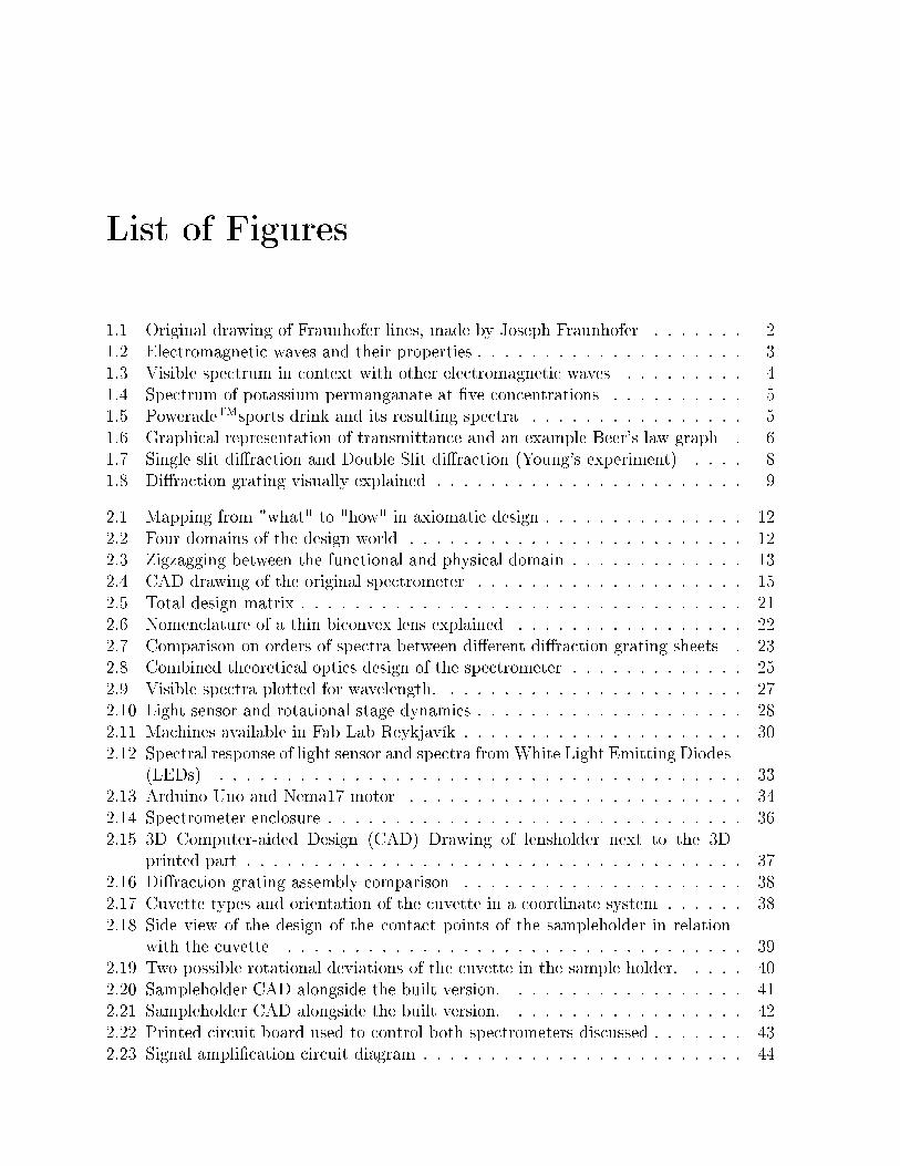
Like mentioned in the introduction, a whole range of commercial spectrometers are avail-able for purchase from a wide variety of sources, ranging drastically in price and cong-urations. Table 1.1 list a few of those devices, along with some details about them. Thislist is in no way intentioned to be exhaustive, but rather show what is available, and inwhat ballpark in terms of price and spectral range.
Many other parameters would normally be considered when one chooses an instrumentfor a specic task, depending on what role the device should ll. Some of the items listedin Table 1.1 are also not standalone devices, so they need a separate computer, light sourceor even other components to be a functioning system. A functional measurement setupcould therefore be much more expensive based on what device is chosen. It should alsobe noted that some of the prices, for instance for Spectrovis 20, are prices for used items,as they were the only ones available at the time of writing.
Along with those commercially available instruments, many articles have been writtenabout builds of low-cost, low-tech spectrometers of various types. Hamilton et al. built afour color photometer with a material cost of $200, reporting labor cost of about $250 perunit if 100 units would be manufactured [3]. Knagge and Raferty built a device with a totalmaterial cost of $195 [5]. Yeh and Tseng built a low-tech spectrometer for a reported costof $20, but their design was based on naked PCB boards and replaceable LED modules,so additional cost would arise if they were to build an enclosure [28]. Cantrell and Inglebuilt the SLIM spectrometer (a ow through device) for $25 per unit [7]. All of these
10 CHAPTER 1. INTRODUCTION
Table 1.1: Lists various commercially available Spectrophotometers
Manufacturer Name Price [$] Type Source RangeVernier SpectroVis Plus 638 Dispersive Vernier webpage 380-950nmOcean Optics USB4000+ UV-Vis 5.000 Dispersive Czegan [2] 200-850nmSpectral Evolution PSP1100 15.000 Dispersive Czegan [2] 310-1100nmBaush & Lomb Spectronic 20 250 Single Beam Ebay 340-950nmThermo Scientic Spectronic 20D+ 2.000 Single Beam Czegan [2] 350-950nmAgilent Technologies Agilent 8453 6.400 Single Beam Conquer Sc. 190-1100nmGlobal Water PhotoLab 6600 7.500 Single Bean w scan Czegan [2] 190-1100nmVarian Inc Cary 100 UV-Vis 2.200 Double Beam LabX 190-900nmVarian Inc Cary 300 UV-Vis 4.400 Double Beam Conquer Sc. 190-900nmShimadzu UV-2600/2700 15.000 Double Beam w scan Czegan [2] 185-900nmPerkin-Elmer Lambda 750 UV/vis/NIR 40.000 Double Beam w scan Czegan [2] 190-3300nm
devices are low cost, but hard to compare against each other because of the fact that theyare designed to full dierent tasks.
1.2.10 Use case
Users of the spectrometers mentioned in Chapter 1.2.9 are normally university chemistryand physics laboratories, even though spectrometers can be used for analytical as well asdiagnostic purposes.
For the spectrometer designed in this project, the target user group is rst year un-dergraduate students of chemistry and engineering in Iceland, with high school studentsin Iceland being a possible secondary target group.

Chapter 2
Design method
Many design protocols and systematic approaches have been developed throughout historyto try to structure the design process and move it away from its trial and error tendency.Here, Nam P. Suh's axiomatic design principle will be studied, and used as a basis for thedesign.
2.1 Axiomatic Design
Axiomatic design is a method developed around 1990 by Nam Pyo Suh at MIT to tryto establish a scientic basis for design. Axiomatic design oers designers a theoreticalfoundation, tools and processes with the goal of improving designs and minimizing trialand error in the design process, as well as a way to determine the best of proposeddesigns [29]. Another goal of axiomatic approach in design was to reduce complexity andprovide a mechanism to make correct design decisions at all levels of the design [30]. Laterpublication by Suh addressed the complexity in design directly [31].
Axiomatic design will be used in the re-design of the spectrometer, as a way to try toensure the best possible solution.
2.1.1 Introduction to Axiomatic Design
Axiomatic design is based on two fundamental axioms. Axioms are truths that cannot bederived but for which there are no counterexamples or exceptions. That is, they cannotbe proven, but there have been no counterexamples that contradict them. These axioms,as presented by Suh are :
Axiom 1 : The Independence Axiom. Maintain the independence of the functionalrequirements (FRs).
Axiom 2 : The Information Axiom. Minimize the information content of the design.
Suh proposed that the best solution of a given problem will be found by representing itin the minimum functional requirements that satisfy the need of the customer, maintainingthe independence of the functional requirements, and choosing the design with the leastinformation content as this will be the best of proposed designs [29].
12 CHAPTER 2. DESIGN METHOD
What wewant
to achieve
How wewant
to achieve it
Figure 2.1: Mapping from "what" to "how" in axiomatic design.
2.1.2 Domains in Axiomatic Design
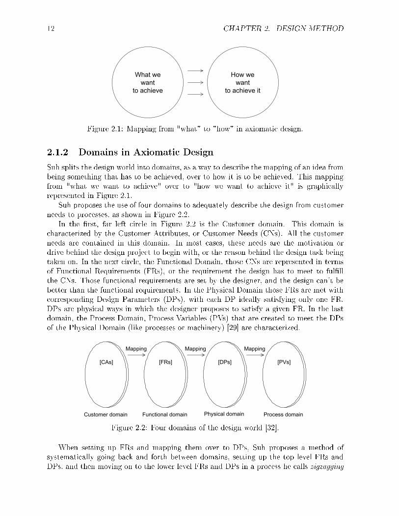
Suh splits the design world into domains, as a way to describe the mapping of an idea frombeing something that has to be achieved, over to how it is to be achieved. This mappingfrom "what we want to achieve" over to "how we want to achieve it" is graphicallyrepresented in Figure 2.1.
Suh proposes the use of four domains to adequately describe the design from customerneeds to processes, as shown in Figure 2.2.
In the rst, far left circle in Figure 2.2 is the Customer domain. This domain ischaracterized by the Customer Attributes, or Customer Needs (CNs). All the customerneeds are contained in this domain. In most cases, these needs are the motivation ordrive behind the design project to begin with, or the reason behind the design task beingtaken on. In the next circle, the Functional Domain, those CNs are represented in termsof Functional Requirements (FRs), or the requirement the design has to meet to fulllthe CNs. Those functional requirements are set by the designer, and the design can't bebetter than the functional requirements. In the Physical Domain those FRs are met withcorresponding Design Parameters (DPs), with each DP ideally satisfying only one FR.DPs are physical ways in which the designer proposes to satisfy a given FR. In the lastdomain, the Process Domain, Process Variables (PVs) that are created to meet the DPsof the Physical Domain (like processes or machinery) [29] are characterized.
Customer domain Functional domain Physical domain Process domain
Mapping Mapping Mapping
[CAs] [FRs] [DPs] [PVs]
Figure 2.2: Four domains of the design world [32].
When setting up FRs and mapping them over to DPs, Suh proposes a method ofsystematically going back and forth between domains, setting up the top level FRs andDPs, and then moving on to the lower level FRs and DPs in a process he calls zigzagging

2.1. AXIOMATIC DESIGN 13
FR 1
FR 1.1 FR 1.2
DP 1
DP 1.1 DP 1.2
Functional domain Physical domain
Figure 2.3: Zigzagging between the functional and physical domain [Note that the imageis modied from its original source] [34].
between domains. Lower level FRs can't be done when higher level FRs and DPs haven'tbeen decided on, so the only way to continue down the hierarchy tree is to zigzag downit in the previously described manner [33]. This is graphically represented in Figure 2.3
Results from this systematic process is what Suh calls axiomatic design. What youare left with after following the process is a description of how customer needs weresystematically satised to end up with a design (be it a system, an artifact or a computerprogram) that fullls all the functional requirements of a customer, with the least amountof trial and error. Or in Suh's own words "Axiomatic Design denes design as the mappingprocess from the functional domain to the physical domain, with the aim of satisfying thefunctional requirements specied by the designer [35]."
Many corollaries and general theorems are also presented by Suh, all relating to thetwo most important axioms in the axiomatic design framework, the independence axiomand the information axiom.
But what exactly do those axioms propose?
To answer this question, design needs to be dened. Design can have dierent mean-ings, depending on elds, but the denition must be broad enough to cover all possiblecases and applications. A design is dened as the mapping from a functional domain toa physical domain, that is, satisfaction of all functional requirements of the customer asthey were specied and understood by the designer [36]. Benavides in his book AdvancedEngineering Design (that has a chapter on axiomatic design) describes this as nding atransfer function from "what we want to achieve" to "how we want to achieve it". Incor-porated in this is the fact that the end product of the design can never be better than thefunctional requirements set by the designer in the beginning [33]. Mapping from what tohow between domains can also be graphically represented like shown in Figure 2.1.

14 CHAPTER 2. DESIGN METHOD
2.1.3 Mapping between domains in Axiomatic Design
Mapping between the domains in axiomatic design can be mathematically representedusing vectors to represent the containings of the four functional domains. In the case ofthe functional and physical domain, this becomes
[FRs] = [A][DPs] (2.1)
Where A is a design matrix that characterizes the given design (How changes in DPsinuence changes in the FRs).
In the case of three FRs and three DPs, the matrix A could be represented as
[A] =
A11 A12 A13
A21 A22 A23
A31 A32 A33
Changes in the design equation are represented as
Aij =∂FRi
∂DPj
(2.2)
Similarly, mapping from the physical domain to the process domain is represented as
[DPs] = [B][PV s] (2.3)
With the B matrix representing the characteristics of the process design.This leaves the designer with three possible types of a design matrices that satisfy
the independence axiom. It can be a diagonal matrix, an upper triangular, or a lowertriangular matrix.
When the design matrix is diagonal, each FR can be satised by a single DP, andthe design is said to be uncoupled. In the case of a triangular matrix, both upper andlower, the independence of FRs can be satised if the DPs are manipulated in a propersequence. In this case the design is described as decoupled. Any other cases will end up inwhat is called a coupled design, where the rst axiom (the independence axiom) cannotbe satised [29].
Suh also describes the ideal design : "An ideal design has the same number of functionalrequirements and design parameters, is uncoupled, and has a null information content.This last characteristic is ensured if the system range falls within the design range" [37].
2.2 Analysis of the MADE-Spectrometer
As previously mentioned in Chapter 1.1, the idea of the project was to re-design andimprove a previously made spectrometer, already designed and built by students of Reyk-javík University. A CAD drawing of their design can be seen in Figure 2.4.
This spectrometer had an optical arm assembly, a rotating table, a motor bracket,diraction grating, a sample holder and a sensor enclosure. Not drawn in the CADdrawing is the circuitry and Liquid Crystal Display (LCD), along with the Arduino board

2.3. DESIGN FOR IMPROVED PERFORMANCE 15
Figure 2.4: CAD drawing of the original spectrometer.
used for data processing. All of the missing components from the CAD drawing weremounted to a Printed circuit board (PCB) specially designed for the purpose.
Fundamentally the idea was to have an optics arm, with a light source on one end,and diraction grating on the other end. A rotational stage moved by a stepper motorwould rotate the light sensor assembly along with a focusing lens, thus selecting a specicwavelength and measure its intensity using a single photodiode. Included in the opticsarm was a sample holder for a 1x1 cm disposable cuvette (a standard size). This cuvettewas to contain the sample to be analyzed. Control PCB including a LCD and a rotaryencoder were used for user interaction with the system. By rotating an encoder, a specicwavelength could be manually selected, and the corresponding absorption then read onthe LCD screen. This way users could do repeated measurements at a specic wavelength(for example for experiments regarding Beer's law), or do multiple measurements over theentire Spectra to nd an absorption Spectra. No automation was programmed into theunit, so manual selection was the only operating mode.
Before building the MADE-Spectrometer the group building it analysed an existingspectrometer in use at the Reykjavík University, namely a device designed by a companycalled Pasco used for measurements in the Physics lab. That device is only used to producespectra for light sources, and does not include a sampleholder or a place to introduce asample.
2.3 Design for improved performance
Fundamentally, the idea behind the spectrometer in this project was to design an aord-able spectrometer with the performance of a sub $5000 commercial unit, have the designcapable of being manufactured in a local Fab-Lab and a basic workshop from easily ob-tainable materials and o the shelf components, while avoiding a black box feel for theend user as previously stated. A basic workshop should have at least a lathe, a bandsawand common metal working tools. The device described will be referred to as the AFL-Spectrometer or AFLS: Aordable Fab Lab Spectrometer. While not a direct redesignof the MADE-Spectrometer, the AFL-Spectrometer can be considered a second iterationin the process of producing an aordable device for laboratory experiments in chemistry

16 CHAPTER 2. DESIGN METHOD
at Reykjavík University, sharing some concepts with its predecessor. In the design of theAFL-Spectrometer, the systematical approach of axiomatic design was chosen to reachthe highest quality design solution satisfying needs while minimizing resources utilizedvia iteration [33],[38].
2.3.1 Design concept
A visible spectrometer is a simple unit in terms of its fundamental principle. White light isbroken into it's components (Spectra) using diraction grating. From there light intensityof a specic wavelength of the spectrum is converted to a voltage value directly related tothe intensity of the light.
After analysing the MADE-Spectrometer, a decision was made to design an enclosed,single beam spectrometer. A photosensitive diode will translate the intensity of light ofa given wavelength into recorded value. Rotary motion will be performed by a rotationalstage consisting of a stepper motor and a rotating wheel with the sensor attached to it,much like the MADE-Spectrometer. Wavelength will be user selected, controlled by arotary encoder. A three color Red Green Blue (RGB) LED with known peaks of wave-length will be used as reference for knowing how to translate rotational motion of thestepper motor to wavelength. By scanning the Spectra and nding these three knownpeaks of wavelength, the translation of movement of the motor to wavelength should bedeterminable by interpolation.
The device should be able to conduct three types of measurements. First o, it canbe used to do experiments relating to Beer's law discussed in Chapter 1.2.5. Secondly itshould be able to measure the intensity of a light source based on wavelength, making itcapable of identifying the spectra (and therefore the type) of the light source and last butnot least it could be used to produce an absorption spectra of a material as has been shownin Figures 1.4 and 1.5. All of these experiments help a student gain an understanding onthe spectroscopic principle and its uses and applications.
2.3.2 Customer needs (CNs)
When working inside the axiomatic design framework, the rst task at hand is acquiringand describing the Customer Needs. In the case of the AFL-Spectrometer, the customeris the faculty and the students that will use the device. Upon verbal communication withsta of the biochemistry and physics courses of the Reykjavík University, their desiresbecame clear. What the customers wanted is an aordable, accurate, durable spectrometerworking on the visible spectrum. Going deeper into examining those conversations, itbecame clear that the motivation is improving teaching capabilities, and the instrumentis the means or the drive of the design. Therefore, the CN is dened as:
CN0 Teach students about Beer's law and diraction of electromagnetic waves on theUV-Visible spectra.
Leading to a zeroth level FRs and DPs presented in Chapter 2.3.3

2.3. DESIGN FOR IMPROVED PERFORMANCE 17
2.3.3 Developing requirements and mapping between domains
When the customer has made clear what it is that he needs, the CNs need to be mappedover to FRs, and from there to DPs. From CN0 we develope the FR0-DP0 pair
FR0 Measure intensity of electromagnetic radiation for a selected wavelength.
DP0 Low-cost measuring device for light intensities on the UV-Vis spectra.
Proceeding to lower level FRs and corresponding DPs. This is done by decomposingand zig-zagging down the domains [29] as has been previously described in Chapter 2.1.1.
Not all of the information about the design is t to become functional requirements.This information is, however, still relevant and needs to be kept track of. This informationis preserved as Constraints (Cs), and presented in corresponding constraint tables. Otherinformation includes optimization criteria presented in Table 2.12. More detail can bestored inside an expanded classical axiomatic design framework, e.g. requirements thatare not functional in their nature, or Non-Functional Requirements (NFRs) [39], but theywere not used in this particular project and are therefore not discussed in detail.
Top level FRs along with their corresponding DPs are described in Table 2.1. Toplevel constraints can be seen in Table 2.2 and the second level constraints in Table 2.3.
Equation 2.4 is the top level design equation.
Table 2.1: Top level FR-DP mapping.
FR DP1 Supply power to components Electronic circuit assembly
2Generate electromagnetic radiation on visiblespectrum
Light source
3 Collimate light from source Collimating lens assembly
4Pass light through constant sample materialthickness
Sample holding assembly
5 Split light into measureble ordered spectraDiraction gratingassembly
6 Measure light intensity Light sensing assembly7 Present data Display assembly
Table 2.2: Top level constraints.
Constraints1 Maximum price $1000.
2Manufacturable in a Fab Lab (Laser cutter, 3DPrinter).
3 Setup time less than 15 minutes.4 Lifespan of a minimum 5 years.5 Usable with outside lightsource.

18 CHAPTER 2. DESIGN METHOD
Table 2.3: Second level constraints.
Constraints4.1 Sample contained in a standard disposable cuvette.6.1 Wavelength selection in 1 and 10 nm steps.6.2 Must handle micro-stepping.6.3 Must handle 2 A of current draw.
FR1
FR2
FR3
FR4
FR5
FR6
FR7
=
X O O O O O OX X O O O O OO O X O O O OO O O X O O OO O X O X O OX O O O O X OX O O O O O X
·
DP1
DP2
DP3
DP4
DP5
DP6
DP7
(2.4)
Right here at the highest level we encounter a lower triangular matrix. This meansthat it would not matter if all of the rest of the design matrices would be diagonal, thedesign will be decoupled.
Going through the matrix systematically we can get some information about the de-sign. From the rst column of the matrix it is evident that the electric circuit assembly(DP1) can have an impact on more of the FRs than just FR1. Without the electroniccircuit assembly FR2, FR6 and FR7 would be aected. How and why? Without the elec-tronic circuit no electromagnetic radiation would be created since the light source wouldnot be powered up, so FR2 is aected by that. FR6 is the measurement of light intensity.Without an electric circuit the sensor and CPU will not run, therefore FR6 cannot befullled by its corresponding DP6 without the electronic circuit assembly. In the samemanner no data is presented on an LCD display without electricity. Only other non diag-onal element in the top level constraint matrix is the element corresponding to the eectthe collimating lens assembly has on FR5. Without the collimating lens assembly thelight can not be split into spectra, and therefore DP3 aects FR5.
Matrix 2.4 can be further decomposed as shown in Tables 2.4 to 2.11. Correspondingdesign equations are Equation 2.5 - 2.12. Optimization criteria are presented at thebottom in Table 2.12.
Table 2.4: FR-DP mapping for power/electronics (FR1).
FR DP1.1 Supply power to lights Light power circuit1.2 Supply power to CPU Light source1.3 Supply power to motor Collimating lens assembly
FR1.1
FR1.2
FR1.3
=
X O OO X OO O X
·DP1.1
DP1.2
DP1.3
(2.5)

2.3. DESIGN FOR IMPROVED PERFORMANCE 19
Table 2.5: FR-DP mapping for light source (FR2).
FR DP2.1 Provide white light Superbright, ultra-white LED
2.2Provide calibration peaks at threeknown wavelengths of the spectra
Three color (RGB) LED
2.3Allow light from an external light sourcein
Hole opening to the outside ofstructure
FR2.1
FR2.2
FR2.3
=
X O OO X OO O X
·DP2.1
DP2.2
DP2.3
(2.6)
Table 2.6: FR-DP mapping for light collimation (FR3).
FR DP3.1 Collimate light Biconvex lens3.2 Align collimator with light path axially Lens bracket
3.3Set distance between collimator and lightsource
Movement mechanism
FR3.1
FR3.2
FR3.3
=
X O OO X OO O X
·DP3.1
DP3.2
DP3.3
(2.7)
Table 2.7: FR-DP mapping for sample (FR4).
FR DP4.1 Keep length of light path through sample constant Sample holder geometry4.2 Keep sample at a xed distance from collimator lens Lens bracket
FR4.1
FR4.2
=
[X OO X
]·DP4.1
DP4.2
(2.8)
Table 2.8: FR-DP mapping for splitting light (FR5).
FR DP5.1 Diract collimated light at an angle Diraction grating sheet
5.2Focus rst order spectra onto a plane at adistance
Focusing lens assembly
5.3Set distance between focusing assembly andsensor
Movement mechanism

20 CHAPTER 2. DESIGN METHOD
FR5.1
FR5.2
FR5.3
=
X O OX X OO O X
·DP5.1
DP5.2
DP5.3
(2.9)
Table 2.9: FR-DP mapping for intensity measurement (FR6).
FR DP6.1 Select wavelength Wavelength selector assembly
6.2Narrow light reaching sensor from spectra toband
Narrow slit in front of sensor
6.3 Measure intensity TAOS TSL2576.4 Process data Arduino Uno
FR6.1
FR6.2
FR6.3
FR6.4
=
X O O OX X O OO O X OX O O X
·DP6.1
DP6.2
DP6.3
(2.10)
Table 2.10: FR-DP mapping for wavelength selection (FR6.1)
FR DP6.1.1 Set desired wavelength value Rotary encoder6.1.2 Control movement of motor Motor controller6.1.3 Move center of light sensor to selected wavelength Stepper motor6.1.4 Prohibit movement of motor ouside of desired range End stop sensor
FR6.1.1
FR6.1.2
FR6.1.3
FR6.1.4
=
X O O OO X O OO X X OO O O X
·DP6.1.1
DP6.1.2
DP6.1.3
DP6.1.4
(2.11)
Table 2.11: FR-DP mapping for data presentation (FR7)
FR DP7.1 Display data LCD Display
FR7.1
=[X]·DP7.1
(2.12)

2.3. DESIGN FOR IMPROVED PERFORMANCE 21
Table 2.12: Optimization criteria.
Optimization criteria2.1 Minimize drift2.2 Minimize heat2.3 Minmize energy use4.1 Maximize repeatability
6.1Minimize stray light reaching intensitymeasurement
Together the entire matrix (simplied using MS Excel) can be seen in Figure 2.5.Printout from Acclaro axiomatic design software can be seen in Appendix A.
7
1 2 3 4xxx
x xx x
xxxxxx
x x x xx x x x x
x1 x x x x x x x x x2 x x x3 x x x x x x x x x x4 x x x
x x x x x x xx
x x7 x x x
4
4
6
32
2
3
1
DPs
FRs
1 2 1 21
4
1 2 3 1 2 3 1
5
3
1
1 2 3
2 3
3121
3
2
4
5
16
2
1
2
3
123
31
12
Figure 2.5: Total design matrix.
At this stage, the CNs, FRs and DPs have been realized in their corresponding do-mains. Axiomatic design has one more domain that can be used for further decompositionof the problem, namely the Process Domain where PVs are described. In the case of theAFL-Spectrometer, no new or exotic processes were needed for the fulllment of the DPsselected. Therefore decomposition into the Process Domain is not described. Fullling

22 CHAPTER 2. DESIGN METHOD
Figure 2.6: Nomenclature of a thin biconvex lens explained [40].
the need of the customer means turning the DPs into physical objects that satisfy theFRs and therefore the CNs or the drive of the customer, thus nishing the design.
2.3.4 Preliminary design analysis
After developing the requirements some analysis was needed in order to understand thephysics of the design problem at hand in order to be able to solve it.
2.3.4.1 Lens dynamics
Looking at the MADE-Spectrometer, and being in the preliminary stages of designingan optical device it was clear that some lenses would be needed to collect, collimate orfocus light at some point. Optical components are normally the most expensive elementsof a spectrometer [3], and lenses are categorized as optical components. Since one of theAFL-Spectrometer's main constraints is cost, expensive lenses were not an option in thebuild. After a research on lenses it was soon discovered that thin biconvex lenses werean attractive option due to their availability and price. A thin lens is dened as onewhere the distance between the two surfaces of the lens along the optical axis is negligiblecompared to its radius of curvature. Nomenclature of a thin biconvex lens can be seen inFigure 2.6.
In Figure 2.6 f is the focal length of the lens, and the point where the rays intersectbehind the lens is the focal point. R1 is the rst radius of curvature and R2 is the secondradius of curvature of the lens, both expressed in meters.
Biconvex lenses come in a variety of congurations, and selection is a matter of ndingsuitable properties for the intended use. For the AFL-Spectrometer a lens with a relativelyshort focal length was expected to be needed. This was due to the fact that the designwas to be compact, and the focal length of the lenses directly inuences the boundary boxof the instrument.
In the MADE-Spectrometer a property of biconvex lenses was used in order to keepthe number of dierent parts of the device to a minumum. What was done was to use twolenses in parallel, or a double lens, and that way split the focal length in half as compared

2.3. DESIGN FOR IMPROVED PERFORMANCE 23
Double lens
Light sensor
600slits/mmFirst orderm=-1
14,51
600slits/mmFirst orderm=1
600slits/mmSecond orderm=2
600slits/mmSecond orderm=-2
14°25°
(a) Spectra for 600 slits/mm sheet.
DoubleFlens
75
LightFsensor
1000slits/mmSecondFordermF=F-2
27,29
1000slits/mmFirstFordermF=F1
1000slits/mmSecondFordermF=F2
48,26
30
1000slits/mmFirstFordermF=F-1
24°44°
(b) Spectra for 1000 slits/mm sheet.
Figure 2.7: Comparison on orders of spectra between dierent diraction grating sheets.
to the single biconvex lens. Placing two identical lenses in parallel cuts the focal lengthof the combined lenses in half compared to its original focal length as can be shown usinga known optical equation called the Lensmaker's Equation [17] :
1
f= (n− 1)
(1
R1
− 1
R2
)(2.13)
In Equation 2.13 n is a unitless index of refraction of the lens (unique for each material).It shows the relations between the focal length, the index of refraction and the radius ofcurvature in a lens. When two lenses are put in parallel the following equation can bederived:
1
fcombined
=1
f1+
1
f2(2.14)
Since the lenses are identical, f1 is equal to f2 and equation 2.14 becomes :
fcombined =f
2(2.15)
So placing two lenses in parallel can have the same eect as having a lens with halfthe focal length.

24 CHAPTER 2. DESIGN METHOD
2.3.4.2 Light source
To produce spectra, the device needed a well characterized and stable light source whichlight could be broken down. LEDs have been used extensively in optical instrumentsdesigned for chemical analysis. Their compact size, low energy consumption, low cost,small drift and low heat emission make them a very attractive choice when designinginstrumentation constrained by cost and size. However, the drawback is that the lightintensity and thus energy provided by a single LED is low, and depending on type, theintensity of light can vary considerably over the range of the visible spectrum. This hasbeen written about extensively by the likes of O'Toole et al. [41] and Dasgupta et al. [42].Due to their low cost and compact size a decision was made to use LEDs as a primarylight source for the AFL-Spectrometer.
2.3.4.3 Producing spectra
Splitting white light into spectra has historically been done by two means. First o aprism was the main mean to break light into spectra, but after the discovery of diractiongrating it came much more popular than the prism. One of the benets of using diractiongrating instead of a prism is that the angle of diraction for a diraction grating sheetcan be calculated precisely using Equation 2.16 [17], as opposed to a prism that splitslight in a nonlinear way as mentioned in Chapter 1.2.1 that cannot be calculated easily.A prism is also very expensive as well as being easy to destroy if it is dropped or hit by ahard object.
d sin θ = mλ (2.16)
In Equation 2.16, d is the reciprocal of number of slits in the grating sheet measuredin meters, θ is the angle of diraction in radians, m is an integer value of the order of theSpectra and lambda is wavelength in meters.
Upon search, prices for glass prisms started at about $50, going upwards with increasedquality. Using a prism would make little sense for the device, so diraction grating waschosen for producing spectra to measure.
Diraction grating sheets are commercially available in dierent congurations. Rollsare sold, for example, in webshops specializing in low-end scientic instruments and labequipment for relatively low amounts of money ($10 being a common price for a few feet).Most commonly available sheets have 1000 slits/mm with 300, 500 and 600 slits/mmalso being widely available. Selecting a grating sheet is essentially a choice of physicalsize of the Spectra, so no "correct" choice exists. Selection can be used to optimize theperformance of the instrument.
To analyze the angles of the rst order Spectra Equation 2.16 and the optical designdescribed in Chapter 2.3.4.4 was used for calculations. Using 400 nm as the beginning ofthe Spectra and 700 nm as the endpoint, a grating sheet with 1000 slits per mm gave anarc of the rst order spectra starting at an angle of 23.6 and ending at 44.4. Using thesame parameters but changing the grating sheet to 600 slits per mm gave an arc startingat an angle of 13.9 reaching over to 24.8. What this meant is that the arc using 1000slits/mm spans roughly 28 mm while the corresponding arc using 600 slits/mm only spans

2.3. DESIGN FOR IMPROVED PERFORMANCE 25
Light9sourceCollimator9lens Double9lens
150
75
Diffraction9grating
Light9sensor
1000slits/mmSecond9orderm9=9-2
27,29
1000slits/mmFirst9orderm9=91
1000slits/mmSecond9orderm9=92
48,26
Sample
30
1000slits/mmFirst9orderm9=9-1
Light
Figure 2.8: Combined theoretical optics design of the spectrometer.
about 14 mm. This meant that the Spectra from the 1000slits/mm is wider, and thusgives a higher possible resolution and will therefore probably be easier to measure.
By selecting fewer slits the Spectra is more compact and starts at a lower angle.Increasing the number of slits widens the Spectra, and moves it further away from its"zeroth-order" bright point in the middle of the optical path. This can be easier explainedgraphically, as is done in Figure 2.7. There, the calculations carried out in this chapterare graphically represented.
2.3.4.4 Optical path
A spectrometer is an optical instrument, and therefore the lenses and path of light arearguably the most important part to understand of the entire design. Other parts arebuilt around the path of light, since the goal is to measure its properties, so the lightpathcannot be blocked. Having selected the optical components, a concept design was madeto gain an understanding of the inner workings of the device before heading on to furtherdesign. Figure 2.8 shows the concept design of the optics of the spectrometer.
Dotted lines show the light from the light source. Before the collimating lens the lightis diverging away from the source, portrayed as diverging in a simplied manner in theFigure. Behind the collimating lens the light is portrayed as parallel rays before endingup in the diraction grating sheet where they are turned into orders of Spectra. From thedouble lens the rays are focused onto a plane away from the focusing lens assembly.
The rst part of the optics is the light source, that as mention in Chapter 2.3.4.2 hasbeen selected to be a LED. A LED can be thought of as a point light source, since thelight emitted from it comes from a very small point.
Next optical device is the collimating lens (chosen as a biconvex lens). Placing a convexlens at a distance equal to its focal length away from a diverging light source collimatesthe light from the said source. Light is considered collimated when its rays are travellingin parallel, and its focal point is said to be at innity. Another way to explain collimation
26 CHAPTER 2. DESIGN METHOD
of light is to say that the diameter of the light beam is constant behind the collimator,that is, the beam is no longer diverging away from the collimator as it was before it.
From the collimator, the light travels through the sample in the sampleholder. Noticethat the sampleholder is not an optical part, but rather an obstacle in the optical path,that is necessary to perform measurements on samples. Design of the sampleholder willbe discussed in more detail in Chapter 2.3.8.5.
After the sampleholder, the light travels through the diraction grating sheet. Fromthere it goes to the last optical component, the double lens (or the focusing assembly).The two lenses in parallel focus the Spectra from the diraction grating sheet onto an arclocated half a focal length away from the double lens assembly and into the light sensor.
2.3.4.5 Light sensor
Many options are available as for sensors sensing light intensity. For this task a lightsensor capable of measuring the intensity of light over the entire visible spectrum wasneeded, but the intensity would only be measured for a narrow band of wavelengths at atime, so there was no need for an array of sensors.
Requirements for the sensor were that it had to be able to translate intensity of lightin the range from about 350-800nm (to cover the visible spectrum) and be as aord-able as possible without sacricing accuracy. Possible choices, and maybe the three mostcommonly used types of light sensors are a photodiode, a photoresistor and a photo-darlington. Sensors most commonly found in LED based chemical analysis devices arephotodiodes [41], and Dasgupta et al. use photodiodes in their spectroelectrochemical owthrough cell [43]. This, coupled with the low price and high availability of photodiodesled to the choice of using a photodiode, rather than any of the other options.
2.3.4.6 Microcontroller
Sensors and LEDs alone cannot process data, so some kind of data processing unit wasneeded to translate the signal from the photodiode to wavelength and display it on theLCD screen. A wide variety of cheap microcontrollers are available, ranging from a fewdollars for single chips, to more expensive bundled solutions like for example the freescaleFRDM-KL25z developement platform, Raspberry Pi and various types of Arduino boards.Constrained by price and to a lesser extent size, selecting a controller for the spectrometeris fairly open, since most of the solutions mentioned above, the usual suspects, are in asimilar price range.
2.3.4.7 Movement of the movement stage
To design the movement stage of the spectrometer, rst an understanding of the dynamicsof its movement was needed. Calculations in Chapter 2.3.4.3 proved that the spectraproduced by the diraction grating produced an arc roughly 30 mm in length. A conceptdrawing of the movement stage dynamics can be seen in Figure 2.10b. Using the samefundamental idea as had been used in the MADE-Spectrometer, backlash free, accuratemovement of the sensor was to be done by connecting the wheels of the movement stage

2.3. DESIGN FOR IMPROVED PERFORMANCE 27
Figure 2.9: Visible spectra plotted for wavelength [44].
together using an elastic shing string under tension. This works much in the same manneras a toothed belt for a fraction of the cost.
Distance of movement of the sensor is controlled by the distance of movement of theshing string, that in turn is controlled by the diameter of the small wheel connected tothe motor. When the motor is rotated, the shing string is moved by a distance controlledby an interplay between the size of the motor wheel and the angle that the motor shaftmoves. What the bigger wheel does is ensure that the sensor is always at an equal distancefrom the focusing lens, and translates the movement of the small wheel over to the sensor.By changing either the size of the motor wheel or the rotation of the motor shaft, a changein the movement of the sensor will be realized. Size of the large wheel is constrained bythe focal length of the double lens, but the size of the motor wheel and the rotation ofthe motor are free variables, by altering those two variables the desired movement of thesensor can be reached.
Looking at Figure 2.9 it is evident that the distance between distinct wavelengthsin the spectra are nonlinear. Therefore, to move to a desired wavelength of the spectracalculations using Equation 2.16 need to be carried out by the processor and turned intoactual distance in accordance with the distance realized between peaks in calibration tomove to a desired location. Looking at this problem and seeing how complex it was, adecision was made to leave that part out for now due to time constraints. Wavelengthselection will be done by hand until the automatic movement has been implemented.
2.3.4.8 Band selection for light sensor
In order to not sense over a wide range of bandwidths at a time, a narrow band of theSpectra needs to be selected and measured, ideally corresponding to 1nm. As mentioned inChapter 2.3.4.7, 1nm of the band has a width of 0.091 mm so optimally the band selectedwould be a perfect slit of that width, having completely parallel edges thus letting throughlight corresponding to only a single wavelength. Figure 2.10a shows the Taos TSL257photodiode used in the MADE-Spectrometer behind an object with a theoretical squareslit at a length of 0.091 mm cut into it.
It is evident from Figure 2.10a that one wavelength only spans a fraction of the actualsensing diode of the sensor package, so it is very important to cover the rest of the sensorfrom other surrounding wavelengths. With a diameter of 1.8mm, the sensor would pickup a span of almost 10nm from the Spectra if no slit was used.

28 CHAPTER 2. DESIGN METHOD
0,091mm
(a) TSL257 and a theoretical slit.
Motor wheel
Large wheel
Fishing wire
Sen
sor
(b) Sketch of the movement stage wheel setup.
Figure 2.10: Light sensor and rotational stage dynamics.
Creating a completely parallel slit of such a small width is a very challenging task initself, even with sophisticated machining tools at your disposal. So for now a medium-density berboard (MDF) sheet with a laser cut slit of a width approximately 0.1 mm willbe used as a mean of covering the sensor. Laser cut edges are never parallel, since thematerial removal using a Epilog laser is done by pulses burning away material, but as arst version, the slit will have to suce.
2.3.4.9 Accuracy
Accuracy of a spectrometer is dened as how able it is to select a correct wavelengthas per instructions from the user. If a wavelength of 440 nm is selected, how capable isthe device of selecting that said wavelength? Conceptually, selecting a wavelength onthe AFL-Spectrometer is going to be done by nding known peaks of wavelength as theyare described by a datasheet from a diode manufacturer. By measuring the distance ofmovement between peaks of the RGB LED a corresponding movement of the motor willbe calculated. This boils down to two factors that need to be accurate for the device asa whole to be accurate.
2.3.4.9.1 Movement accuracy
Movement accuracy is the ability of the device to move a correct distance each and everytime it is asked to do so. If the motor does not move a correct distance, there will be adiscontinuity between the displayed wavelength value and the actual value of the positionof the sensor.
2.3.4.9.2 Wavelength selecting accuracy
Wavelength selecting accuracy will be aected by how close to the datasheet of the RGBLED the actual peak values of the LED are. Peaks of the diode can vary, but a hard codedvalue needs to be selected as the position of the peak, and calculations and therefore move-

2.3. DESIGN FOR IMPROVED PERFORMANCE 29
ment of the motor will be o by an amount relating to the errors in the wavelength betweenthe actual and the theoretical peaks of the diode.
2.3.4.10 Repeatability
Repeatability is dened as a systems ability to perform in the same way when identical,repeated measurements are being made on the device. Repeatability is arguably the mostimportant to get right of the three big pillars, accuracy, repeatability and resolution. Ifyou know how consistent, or repeatable your measurements are, you can calibrate for theaccuracy. If you ask it to move to wavelength of 440 nm and it goes to 450 nm each andevery time, you can adjust for 10 nm that the device is consistantly o. It is harder to doif you get unpredictable results due to low repeatability.
2.3.4.11 Resolution
Resolution of the spectrometer is based on how small of a wavelength band it can select,and how accurately it can measure a given band. Resolution of the device is also boundby the A/D converter being used to produce the measurements. With a more sensitiveA/D converter, smaller changes in the output signal of the sensor can be sensed and it issaid to have a higher resolution.
2.3.4.12 Error analysis
2.3.4.12.1 Optical path error
Errors in the optical path of the instrument can be broken down into a few possiblesources.
First o, the lensholders are manually located by the user inside the body of the unit,and secured in place with wing nuts. Guiding slits designed into the structure of thedevice help locate the lenses, but keeping them completely parallel to the light source,and at an exact distance is hard. This will inevitably be the cause of some error. Distancefrom the source matters more for the collimating lens than the double lens.
Another possible source for error is the use of soft diraction grating sheet, instead ofusing a hard solid glass piece like common in more high-end commercial devices. Gratingsheets as used in the AFL-Spectrometer are made from sheets of plastic, and can thus bebent into shape and rolled up. This is what makes them so aordable, but comes with adrawback. Cutting it up and placing it between two MDF plates does not ensure that thediraction grating is completely vertical. It could also bulge or bend, as another sourceof error. Both of these errors could be overcome by buying a precision made diractiongrating sheet from glass.
Lastly, and maybe the biggest concern and source of error in the optical part of thedevice is the stray light. While other error sources pose problems, they stay consistentbetween measurements and even between measurement runs or uses. Stray light canchange based on time of day, changed lighting in the room due to unnatural factors suchas doors being opened or a variety of other sources. A mitigation strategy against this is

30 CHAPTER 2. DESIGN METHOD
(a) Makerbot Replicator 2 [45]. (b) Epilog 24 mini laser cutter [46].
Figure 2.11: Machines available in Fab Lab Reykjavík.
to seal all bounds with masking tape to try and ensure that no stray light enters the lightsensor.
2.3.4.13 Drift
Drift is dened as a change over a period of time in output measured value when nochange is being made to the sample being measured. This could include a measured valueof absorption changing with time when a blank sample is intentionally left for an extendedperiod of time in the instrument. Drift can occur for many reasons, and will inevitablyhappen. Knowing the main sources for drift is important when working with scienticinstruments to be able to accurately interpret results.
2.3.4.13.1 Sources of drift
Drift in spectrometers can be a result of dierent factors. Historically, the biggest driftfactor was due to the change in the behavior and characteristics of incandescent lightsources over time, that is the degradation of the light source. Many older spectrometershad to be turned on and the light source allowed to heat up before they could be used toproduce repeatable results.
Another source of drift is the breakdown and change in composition and properties ofchemical solutions in the presence of light. What is meant by this is that some solutionsof materials are sensitive to light, and therefore the absorptivity of the solution changesas it is exposed to light for extended periods of time. This, however, should not be a bigconcern when analyzing the drift for instrument, since the drift can be measured with nosample present in the instrument.
2.3.4.13.2 Drift due to light source
Drift caused by the LED's is due to the fact that they fade with time, that is, theirintensity weakens. Lifetime of LED's is a topic that has been studied to great lengths.

2.3. DESIGN FOR IMPROVED PERFORMANCE 31
It is dened as the point where the intensity of the light from the diode goes under 70%of the intensity it produced when new. This is dierent from the lifetime of an incan-descent lightbulb that normally fails absolutely, while also fading in brightness along itslifetime. Lifetime of a LED is considered to be short if under 10.000 hours, and veryshort if under 5.000 hours [47]. If the degradation is fast enough, it will result in visibledrift over the measurement time (one lab session). Other factors, such as heat build upinside and around light sources can also cause drift due to changed mechanical propertiesof materials in the light source, but is a not a concern factor when working with LED's.
2.3.5 Structural material selection
Having analysed the physics and background for the AFL-Spectrometer, material selectionwas the next logical step.
For the device to be manufacturable in a Fab Lab, material selection is narrowed tothe materials the machines at the Fab Lab can use. Fab Lab Reykjavík has four machinesrelevant to the production of the AFL-Spectrometer. These machines are two Epilog Mini24 - 40 Watt laser cutters, a Makerbot Replicator 2 - 3D printer and a Replicator 2X -3D printer.
Epilog Mini 24 can cut wood, wood based materials, paper and plastics along withother lesser dense materials. Replicator 2 and Replicator 2X can print using PolylacticAcid (PLA) and Acrylonitrile butadiene styrene (ABS) thermoplastics respectively. Bothdevices can be seen in Figure 2.11.
For the structural material the choice was between wooden materials, or Plexiglas(PMMA) or other plastics. Plastics are generally more expensive than wooden materi-als. Plexiglas also normally comes in glossy nish, not ideal for the inside of an opticalinstrument, due to light scattering and mirror eects. Other plastics were considered to ex-pensive for the project. This left the designer with only wooden materials to choose from.Plywood is relatively aordable and readily available, but the lower grades of plywoods(that would be in the price range for this project) can include defects like knots and plugs.This lead to the selection of MDF as structural material. MDF is an engineered woodproduct made from wood bers from both hard and softwood, bound together under highpressure and heat using wax and resin binding. MDF is more dense, and more uniformthan plywood, readily available, and very aordable. A sheet of 1x1.5 m costs around$12 in Iceland. It, however, has the drawback (like other wooden materials) that it isdynamic. Moisture and temperature change the behavior of the material (it expands andcontracts), but it was obvious that some sacrices had to be made on material selectionbecause of machining and pricing constraints. Contraction and expansion also happenson a slow enough scale that it will not have signicant eects on the measurements of theunit.
Parts of the instrument were 3D printed using the Replicator 2. Since the lamentused by that machine by default is PLA, there was no choice for other materials andtherefore no actual material selection. This, however, had not much signicance in thiscase, since the plastic type was not critical. This is due to the fact, that in the design thereis no structural integrity needed from the plastic parts due to the nature of their designand placement in the unit. PLA was also available in black color, as opposed to the ABS

32 CHAPTER 2. DESIGN METHOD
used for the Replicator 2X unit which Fab Lab Reykjavík only stocked in white color.Black plastic is a better choice in the optical path, since it scatters less light than whiteplastic. This lead to the parts being manufactured from black PLA using the MakerbotReplicator 2.
2.3.6 Physical component selection
Component selection goes hand in hand with other parts of the physical design of theinstrument. At the beginning of the design, the designer has a rough idea of whichcomponents are needed to fulll the CNs, but maybe not their exact specications or otherproperties such as size constraints. Therefore the component selection can be dynamicduring the design process as a better understanding of the problem is gained and thedesign matures.
2.3.6.1 Lenses
Like with other components, many dierent congurations were available for lenses. Afteranalyzing what performance was needed from the lenses, see Chapter 2.3.4.1, a lens witha focal length of f = 15 cm was chosen. It has a diameter of 38 mm and a thickness ofroughly d = 4 mm. This lens was chosen because of its relatively modest price tag of $6a piece, and it being widely available upon search on Amazon.
2.3.6.2 Grating sheet
After going through the analysis in Chapter 2.3.4.3 the obvious choice for a diractiongrating sheet was a plastic grating sheet with 1000 slits per millimeter. It is aordable,available and strikes a good balance between size of spectra and distance between ordersof spectra. Searching for glass grating sheets for comparison it was evident that it wasnot a viable option. Prices started at $50 for a single piece in the low price range, goingup to $250 in the high end range.
2.3.7 Electrical component selection
2.3.7.1 Light sources
White LEDs come in a wide range of available sizes, from surface mount and snub-nose5mm housing to arrays and strips to name a few. For the AFL-Spectrometer a classic 5mm(T-1 3/4) LED was chosen and bought from an online company named SuperBrightLEDS1.A few dierent types of LED were bought and tested. A spectral graph for one of theLEDs can be seen in Figure 2.12b.
As a reference for translation of rotational movement of the movement stage over towavelength of the Spectra, another LED was designed into the device. This LED is anBL-L515RGBW RGB diode, capable of emitting not only white light, but all possibleRGB color variations. Most importantly though, it has distinct peaks of three colors,
1www.superbrightleds.com

2.3. DESIGN FOR IMPROVED PERFORMANCE 33
(a) Spectral response of TAOS257 photodiodeplotted against wavelenght λ [48]. (b) The spectra of the white RL5-W6030 LED.
Figure 2.12: Spectral response of light sensor and spectra from White LED
namely red, green and blue. These peaks are denoted in the LEDs datasheet2, and byletting the movement stage scan and nd those peaks while keeping track of the rotation,rotational movement of the motor can be translated to wavelength of light in a singlecalibration pass.
Along with having a white LED and a RGB LED, a functional requirement was thatthe instrument would have to accommodate an outside light source. Many physics labshave gas-discharge lamps with replaceable bulbs that can also be used as a light sourcefor a spectrometer. These gas lamps have a dierent spectrum than a white light, butalso have the benet of having been studied extensively throughout history. Thereforethe spectral properties of many gases is very well known. For this reason, in addition tothe LED's, a hole was designed on the spectrometer body structure to be able to let lightfrom an outside source in, mainly focusing on the use of gas-discharge lamps. This holewould then be covered when the outside lightsource would not be in use. Many of thosegas lamps do have very sharp peaks at known wavelengths, and could thus, as well asthe RGB diode, be used as calibration points when translating rotational movement towavelength.
2.3.7.2 Light sensor
After analyzing the need for the light sensor in Chapter 2.3.4.5 a few possible candidateswere found. TAOS TSL257 fullled the requirements set up, being capable of convertinglight to voltage in the range from roughly 300-1100nm according to its datasheet [48],running on 2.7-5.5V, while costing under $5. A graphical representation of the spectralresponsivity of TSL257 can be seen in Figure 2.12a.
TSL257 is not only a photodiode, but rather a package containing an op-amp, a resis-tor, a photodiode and a capacitor. Its output is a DC signal with a voltage proportionalto the value of light reaching it as compared to its saturation. That is, when saturation
2http://www.adafruit.com/datasheets/BL-L515.PDF

34 CHAPTER 2. DESIGN METHOD
(a) Arduino Uno [50]. (b) Nema 17 stepper motor [51].
Figure 2.13: Arduino Uno and Nema17 motor.
is reached the sensor outputs a DC signal equal to its feed voltage. When fed with 5Vsignal, 50% saturation gives an output of 2.5V DC, while saturation is a 5V DC signal.
2.3.7.3 Microcontroller
A Arduino Uno board is more than capable of handling both the data manipulation fromthe photodiode, as well as being able to control the rotation of the motor, calibration ofthe device as well as other pre-programmed tasks needed for a functioning spectrometer.Costing $25, the Uno board is a solid option. Having worked extensively with Arduino inthe past and knowing the development platform, Arduino was the most obvious choice. Allthe code for the MADE-Spectrometer was also developed for Arduino Uno, so re-cyclingcode from that project could save time and help simplify the programming.
Arduino Uno runs on the ATmega328 microcontroller. The operating voltage of theboard is 5V, and it runs at a clock speed of 16MHz. Available memory is 32KB (Flash,of which 0.5 is allocated for the bootloader), 2KB SRAM and 1KB EEPROM. It has 14digital I/O pins and 6 analog input pins with a 10 bit resolution. Communication to acomputer goes on through a USB port on the board, from which the program to run onthe ATmega328 chip is sent through serial communication [49]. A picture of the ArduinoUno board can be seen in Figure 2.13a.
2.3.7.4 Motor
When working with rotational movement that needs to be precise while also being con-strained by cost, stepper motors are an obvious choice. They oer stepwise rotation thatcan be controlled very repeatibly when the torque applied to the motor is far from itsmaximum rated torque. stepper motors are available in a very wide range of sizes andcongurations. Selecting a unit depends on the resolution needed, geometric constraintsand maximum torque requirements to name a few. stepper motors require a fairly sophis-ticated control mechanism, or a driver, since they are driven by a dynamic sequence ofpulse width modulated signals.

2.3. DESIGN FOR IMPROVED PERFORMANCE 35
For the MADE-Spectrometer, a NEMA 17 stepper motor capable of 200 steps perrevolution had been chosen. This size motor is very popular for hobby projects as wellas commercial applications of all sorts, and is therefore very widely available and veryaordable, costing only $25. 200 steps per revolution gives a rotational resolution of 1.8,but the resolution can be increased by microstepping the motor as needed, even downto eight of a step depending on the driver. Microstepping a motor has the drawback ofdecreased torque, but the torque needed to move the sensor is so low that it is a matterof no concern here. For the AFL-Spectrometer the same type of motor was used as forthe MADE-Spectrometer, due to the reasons mentioned before. A picture of a NEMA17stepper motor can be seen Figure 2.13b.
2.3.7.5 Motor controller
As previously mentioned, stepper motors need fairly sophisticated controllers to run dueto nature of motor design, especially when working with parts of steps, or what is referredto as microstepping.
For the AFL-Spectrometer no real torque, speed or noise constraints for the motor ap-ply. Moving the rotating part takes little to no torque, since it is very light and the frictionbetween the PEHD bushing and the MDF material used for the body is very low. Speed isnot signicant, since the Spectra only spans about 20 of a circle, corresponding to about30 mm arc like previously mentioned. Even if it only moves at 0.5 mm s−1, moving overthe entire Spectra would only take a minute, which is perfectly acceptable. As for noise,limiting it would be benecial, but this size motor does not have the ability to produceunacceptable levels of noise (damaging to the users hearing). For the AFL-Spectrometerthe most important constraint is vibration. When stepper motors are driven at highspeed at maximum stepping size, vibration is noticable. Using microstepping and goingslower drastically minimizes vibration. Therefore the characteristics of microstepping areall suitable for the AFL-Spectrometer.
Any stepper driver capable of currents up to 2 A, with microstepping capabilities wouldbe suitable for the project. Chosen for this project was a driver made by Polulu robotics &electronics named md09b. It is an integrated circuit using Allegros A4983 microsteppingbipolar stepper motor chip, capable of 1/16th steps, handling 2 A per coil of currentwith operating voltages between 8 − 35 V. This circuit also includes over-temperatureprotection, under voltage lockout along with a crossover current protection. The driver ismanaged by the Arduino Uno.
2.3.8 Breakdown of design
2.3.8.1 Enclosure
To block as much stray light as possible, the AFL-Spectrometer is designed as an enclosedunit. To get to the inside of it, the top part is split in two, with the bigger half hinged toopen it up to get to the optical components. Having the unit enclosed allows users to domeasurements in a fully lit room, as opposed to having to turn o all light in the roomwhere the device is being used. As discussed in Chapter 2.3.5, the enclosure is designed

36 CHAPTER 2. DESIGN METHOD
Figure 2.14: Spectrometer enclosure.
out of MDF. It is only made from one thickness of MDF, 4mm, for simplications sake.To keep the enclosure together a combination of keys and snap-in fasteners designed intothe basic parts are used, as opposed to bolted, riveted or any other types of mechanicalconnections. Avoiding bolted connections lowers the overall number of parts. This is atype of design decision aimed at increasing simplicity and therefore information contentof the design, relating directly to Axiom 2 of the axiomatic design principle.
To further block light from getting in through joints on the body, all of them weresealed with duct tape. Figure 2.14 shows the assembled (and taped) unit.
2.3.8.2 Light holder
In front of the optical devices is the light holder. There a hole is lasercut to hold the twoLEDs that generate light for the device. The light holder is also designed in a way thatoutside light can shine through it in accordance to Constraint 5 as set up in Table 2.2.
2.3.8.3 Lensholder assembly
Three lenses are used in the AFL-Spectrometer. One lens is used to collimate the lightfrom the light source, as previously mentioned, and two lenses in parallel are used to focusthe Spectra from the grating sheet into the light sensor.
It was soon realized that the geometry of the lensholder would be a fairly complex one.It had to support the lens, keep it axially aligned with the light path, keep the distancebetween the source and the lens xed at a correct length, while allowing some adjustmentfor the user, to make up for possible errors in the machining and assembly. This led to thechoice of designing the lensholders to be manufactured by a 3D printer. The geometricshape of the lensholder was made using a 3D CAD software, and printed on the MakerbotReplicator 2 mentioned in Chapter 2.3.5. Finished CAD design alongside the actual 3Dprinted part can be seen in Figure 2.15.

2.3. DESIGN FOR IMPROVED PERFORMANCE 37
(a) 3D CAD model of double lensholder withlenses. (b) 3D printed single lensholder with lens.
Figure 2.15: 3D CAD Drawing of lensholder next to the 3D printed part.
Two versions of the lensholder were designed and built, one for a single lens and anotherone for the focusing lens (double lens assembly). They were identical in all ways, exceptfor the double lensholder having two lens slots instead of a single one.
As can be seen in Figure 2.15a, both slots in the lensholder are identical, as well as thelenses themselves. This should ensure that the optical axis of both lenses line up, whilealso lining up with the optical axis of the collimating lens. No fasteners are needed tokeep the lenses in place, since the lensholder is designed so the lenses snap in place andsit rmly in their groove without assistance, taking advantage of the material propertiesof the plastic material used.
2.3.8.4 Diraction grating assembly
One of the most important individual pieces of the device is the diraction grating sheet.Without the grating sheet, the white light would not be diracted, and therefore noSpectra would be visible to be measured.
For protection of the grating sheet and to position it correctly inside the optical path,the sheet was designed into a frame of two MDF plates. The assembly is then slid intoplace using pre-cut slits on the spectrometer body, positioning it precisely. To keep theframe together, three hexagonal bolts and nuts are used to hold it together. Figure 2.16shows the CAD drawing of the diraction grating assembly alongside the manufactureditem.
As discussed in Chapter 2.3.6.2 the diraction grating sheet was bought in a roll froma scientic online shop. It was then cut to shape and placed inside the protective assemblyas parallel as possible to the sides of the assembly.
2.3.8.5 Sampleholder
Based upon the design matrix and examination of the light path, it is clear that a high-information element lies in how the sample will be held, due to its eect on the spectra.Samples used in the AFL-Spectrometer will be liquid solutions. Solutions need to be
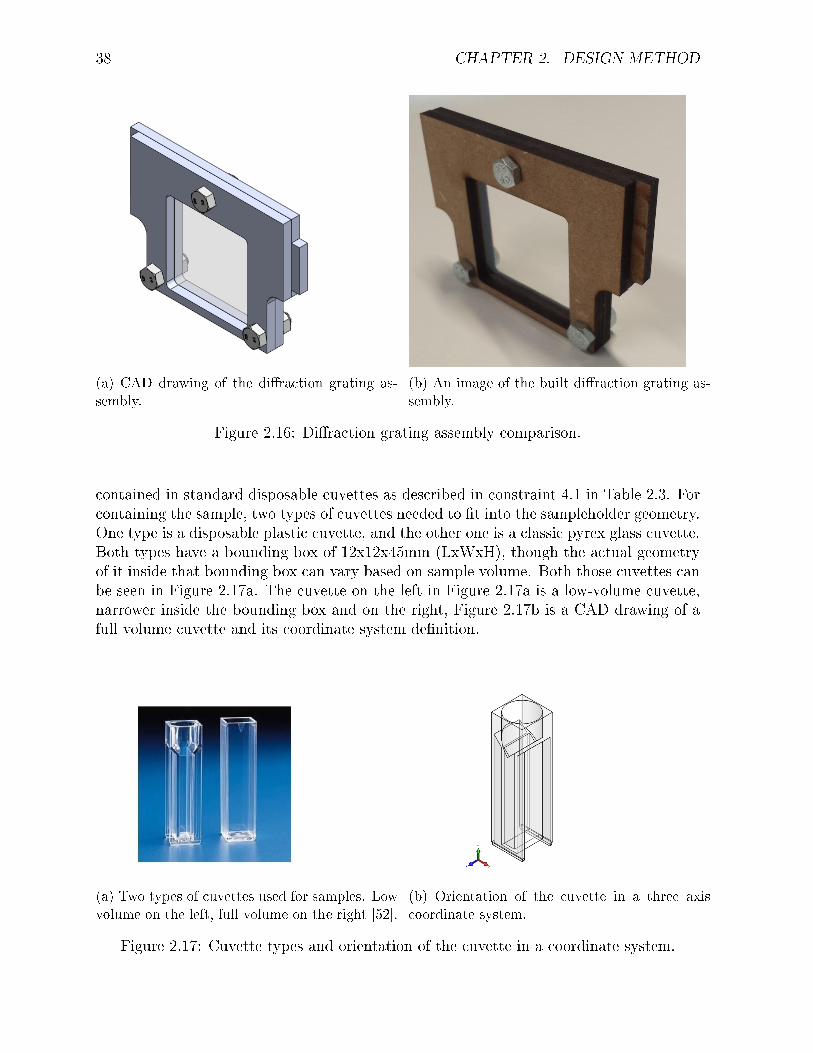
38 CHAPTER 2. DESIGN METHOD
(a) CAD drawing of the diraction grating as-sembly.
(b) An image of the built diraction grating as-sembly.
Figure 2.16: Diraction grating assembly comparison.
contained in standard disposable cuvettes as described in constraint 4.1 in Table 2.3. Forcontaining the sample, two types of cuvettes needed to t into the sampleholder geometry.One type is a disposable plastic cuvette, and the other one is a classic pyrex glass cuvette.Both types have a bounding box of 12x12x45mm (LxWxH), though the actual geometryof it inside that bounding box can vary based on sample volume. Both those cuvettes canbe seen in Figure 2.17a. The cuvette on the left in Figure 2.17a is a low-volume cuvette,narrower inside the bounding box and on the right, Figure 2.17b is a CAD drawing of afull volume cuvette and its coordinate system denition.
(a) Two types of cuvettes used for samples. Lowvolume on the left, full volume on the right [52].
(b) Orientation of the cuvette in a three axiscoordinate system.
Figure 2.17: Cuvette types and orientation of the cuvette in a coordinate system.

2.3. DESIGN FOR IMPROVED PERFORMANCE 39
CG
1
2y
z x
Cuvette
Light path
Figure 2.18: Side view of the design of the contact points of the sampleholder in relationwith the cuvette.
For maximum repeatability, the center of mass of the cuvette was compared to the de-sired alignment translation axes (~x, ~y, ~z) and rotational angles around those axes (θx, θy, θz).For an alignment reference, ~y is normal to gravity and ~z is the path of travel for the light.Critical movement directions are θy, θx, ~y and ~x. θy and θx result in elongation of the lightpath through the sample, see Figure 2.19, while the other movements move the cuvetteout of the path of light inside the device.
Traditional holding mechanisms use spring loaded coil spring or exure nger mecha-nisms; a sample is inserted into an aperture to interface with the exures. Some spectrom-eter models require the additional step of locking the sample in place to increase preload.The commercial units used for comparison (see Section 3.2) had a plastic cassette for thecuvette that slid into a chamber with a stamped-metal exure. Here a similar design wasused, but the xture design was reduced to a minimum number of mechanical elementsthat would be easily manufactured in the Fab Lab.
Figure 2.18 shows the design concept of the sample holder. One spring-loaded shaftand four static shafts align the cuvette along the optically-at sides. These contact areasensure repeatable positioning of the sample focusing on eliminating movement in thesamples critical movement directions. Constraining only these four degrees of freedomonly needs ve shafts thus keeping the information content of the design to a minimumas per Axiom 2: adding more restraints would only add unnecessary complexity. A CADrendering of the physical implementation of the concept in Figure 2.18 can be seen inFigure 2.20a. Other directions are limited by laser-cut MDF features because they do notsignicantly aect the light path.
It should be noted that it is unrealistic to assumes that the cuvette is or will becompletely parallel to the lightsource in praxis. What is to be done is to ensure it to be asparallel as possible inside the nancial constraints, and have make sure the cuvette goesinto the holder in a repeatable manner. Errors in the pathlength are manageable as longas they stay consistently o and repeatable. This holds true for other parts of the designas well.
Completed CAD of the xture can be seen in Figure 2.20a.

40 CHAPTER 2. DESIGN METHOD
(a) Cuvette rotated around θy. (b) Cuvette rotated around θx
Figure 2.19: Two possible rotational deviations of the cuvette in the sample holder.
Figure 2.18 shows the cuvette in the sampleholder, the location of the axles retainingit, the center of gravity and its rotational points. As can be seen, on the left side it iscontained by two axles in contact. A axle at the bottom ensures that the cuvette is insidethe beam in the ~y. Lastly, on the right side of the cuvette is an axle that is springloaded.This axle is located between the two rotational points of the cuvette with the center ofmass in between them, therefore making it stable and keeping it steady in the holder. Itis placed as high as possible to not block the path of light through the sample. These fouraxles are enough to retain the sample in the most critical directions when the sampleholderis locked and loaded. A side eect of the two axles on the front is that the sample is at axed distance from the light source at all times when inside the holder, and the lowest axleensures that the height is correct. Those last two are non-critical movements as previouslymentioned in the text, but they come as free extras due to the geometric design of theholder. Movement in the ~(x) is very loosely constrained by the springs acting on thespringloaded axle, enough to always keep the sample inside the light beam, more thanenough to full all functional requirements without any additional information content.
2.3.8.6 Movement stage
The movement stage is comprised of two wheels. One machined PEHD wheel is directlyattached to the output shaft of the stepper motor connected to another bigger wheel thatis lasercut from MDF. A light sensor is mounted to the bigger wheel using an enclosurealso made from lasercut MDF. Connection between the wheels is through a nylon shingstring under tension, as a means of eliminating backlash when rotational directions arechanged. A sketch of the setup can be seen in Figure 2.10b.
For the Spectra to be measured in focus, the light sensor must be positioned one focallength, 7.5 mm, away from the double lens, therefore putting some constraints on thephysical size of the bigger wheel. In the case of the smaller wheel, the size of it is whatdecides the movement in each step that the stepper motor takes. As the name implies, astepper motor moves in steps. This particular one has 200 steps per revolution, and hasan output shaft with a diameter of 5 mm. As mentioned, this part of the movement stagedecides the distance of movement in each step of the motor, so this has to be matched
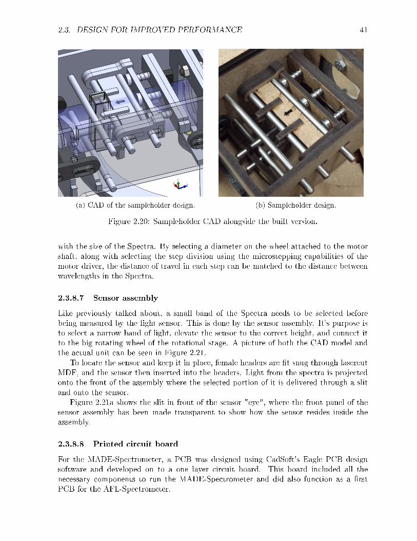
2.3. DESIGN FOR IMPROVED PERFORMANCE 41
(a) CAD of the sampleholder design. (b) Sampleholder design.
Figure 2.20: Sampleholder CAD alongside the built version.
with the size of the Spectra. By selecting a diameter on the wheel attached to the motorshaft, along with selecting the step division using the microstepping capabilities of themotor driver, the distance of travel in each step can be matched to the distance betweenwavelengths in the Spectra.
2.3.8.7 Sensor assembly
Like previously talked about, a small band of the Spectra needs to be selected beforebeing measured by the light sensor. This is done by the sensor assembly. It's purpose isto select a narrow band of light, elevate the sensor to the correct height, and connect itto the big rotating wheel of the rotational stage. A picture of both the CAD model andthe actual unit can be seen in Figure 2.21.
To locate the sensor and keep it in place, female headers are t snug through lasercutMDF, and the sensor then inserted into the headers. Light from the spectra is projectedonto the front of the assembly where the selected portion of it is delivered through a slitand onto the sensor.
Figure 2.21a shows the slit in front of the sensor "eye", where the front panel of thesensor assembly has been made transparent to show how the sensor resides inside theassembly.
2.3.8.8 Printed circuit board
For the MADE-Spectrometer, a PCB was designed using CadSoft's Eagle PCB designsoftware and developed on to a one layer circuit board. This board included all thenecessary components to run the MADE-Spectrometer and did also function as a rstPCB for the AFL-Spectrometer.

42 CHAPTER 2. DESIGN METHOD
(a) CAD of the sensor assembly. (b) Built sampleholder.
Figure 2.21: Sampleholder CAD alongside the built version.
It was designed as a shield for Arduino Uno, with male headers connecting to thefemale headers of the Uno board. A barrel jack, rotary encoder and a LCD are alsoconnected directly to the PCB, so all electronic components are included in the assembly.A picture of the MADE-Spectrometer PCB can be seen in Figure 2.22.
2.3.8.9 Software
Software or code used in the AFL-Spectrometer was the same code that had been devel-oped for the MADE-Spectrometer. Since the goal of the project was to focus on axiomaticdesign principles and mechanical design the software part of the device was left for oth-ers to explore in greater detail. All of the code was developed using the Arduino IDEdevelopment environment. The software used in the project is available upon request.
2.3.9 Realizations and modications in the design phase
Even though axiomatic design is aimed at minimizing the iteration and wasted eort inthe design phase, it is hard to design mechanical objects and get all decisions correcton the rst go. Concepts and things that seemed fairly intuitive beforehand can alsobe debunked, and some discontinuity can exist between the theoretical world and thepractical application of it. Here some of the iterations, problems and re-designs of thedesign will be discussed.
2.3.9.1 Movement stage iterations
In the rst version of the movement stage, the wheel carrying the sensor was elevatedslightly from the oor or the bottom of the device. After building a prototype and ddling

2.3. DESIGN FOR IMPROVED PERFORMANCE 43
Figure 2.22: Printed circuit board used to control both spectrometers discussed.
a bit with the wheel, it became evident that not supporting the wheel by any means fromthe bottom would result in it wobbling badly, and therefore the sensor assembly would beable to move considerably as a result. To compensate for this, the wheel and the bushingwas re-designed so that the wheel would be supported by the bottom of the enclosure.This eliminated the wobbling of the sampleholder and therefore took care of the problemconcering the wobbling.
2.3.9.2 Sampleholder iterations
Since the sampleholder was the biggest impact factor on the design, much time was devotedto getting the design of it just right.
The rst iteration had four independent spring loaded pins connected to a 3D printedtriangle supporting the sample. This proved very hard to adjust and the sample was veryprone to getting stuck in the sampleholder. After seeing that four individual preloadswere probably not the way to go, the route of using axles/shafts with only one preloadwas taken. This idea was taken to the drawing board, and ended up being the solutionused.
2.3.9.3 Signal processing
Turning a signal from the sensor to a displayable intensity or value through an A/Dconverter can oftentimes be dicult, and every designer that has built a measuring deviceknows that getting it right can be tricky.
In the rst trial measurements of the device, no signal processing or ltering of anykind was applied to the signal before measuring it, resulting in a ickering readout becauseof noise. Another problem that presented itself was, that during normal measurementsthe maximum readout from the A/D converter was about 600 bits from the potential1023. What this meant is that the A/D converter wasn't being fully utilized and thusresolution was being lost. To compensate for these two things an amplication circuitwith a lter was built to amplify the signal from the sensor. By using an operational

44 CHAPTER 2. DESIGN METHOD
R1
R2 R3
Vin
Voutlm324C1
Figure 2.23: Signal amplication circuit diagram.
amplier the signal from the sensor was amplied so that maximum measurements innormal operations came closer to the maximum 1023 bits of the converter (5V in the caseof the Arduino).
Amplifying the signal above 5V could pose damage to the input port on the Arduino,as voltages over 5V would be realized when the lid on the spectrometer would be opened.To make sure this would not happen the feed voltage to the amplier was limited so thatthe maximum amplied signal could reach 5V but never exceed it.
Many well known amplifying circuits could have been chosen, but the one used wasa classic non-inverting amplifying circuit using an LM324 op-amp. Analysing the signalusing a spectroscope showed that the noise on the signal was of higher frequencies (5 −−20 kHz) so a classic low-pass RC lter was added before the op-amp to remove the noise.Values used for the lter were a resistor with a resistance of 820 Ω and a capacitor withcapacitance of 100 nF. For the non-inverting amplier circuit, various amplications weretested during by switching out the resistors in the circuit. This is discussed further inChapter 3. This improvement stabilized the readout of the signal tremendously and abetter utilization of the A/D converter was evident, since maximum readings went froma maximum of about 500 bits for the strongest signals up to around 1000 bits, thus fullyusing the potential of the converter. Instead of ickering on a span of about 10 bits thesignal went to ickering on about 3 bits, making the readout a lot easier. Circuit drawingsfor the lter and the amplication circuit used can be seen in Figure 2.23.
2.3.10 Limitations of the design
Working inside a set of constraints also means that the design will be limited in someways. Having gone the route of manufacturing the unit in a Fab Lab from MDF meansthat the unit will not withstand massive liquid spills. Spilling on it will change the shapeof the MDF and cause it to deteriorate. When working with comparable commercialunits (presented in Chapter 3.2) it became clear that liquid spills and corrosiveness isa universal problems when working with devices that measure liquid solutions. Thosecommercial units both showed wear due to the spill of chemicals on them over time.

2.3. DESIGN FOR IMPROVED PERFORMANCE 45
Another limiting factor of the device is the A/D converter of it. Choosing an ArduinoUno platform as the processing unit meant a maximum resolution of 10 bits for the A/Dconversion. With a higher resolution A/D converter more accurate measurements couldbe made on the device.
Being built from MDF, the device is not as sturdy as devices built from strongerstructural materials, but for normal use in a laboratory setting, MDF is most certainlysturdy enough for the device to serve its educational purpose.
2.3.11 Cost
Total cost of parts came in at roughly $245, with the power supply being the singlemost expensive part and the Arduino Uno coming in second. Since most of the partswere sourced from vendors located in the United States, shipping, handling and tax hasto be added to the total amount to get a correct price for the items when in Iceland,but the overall amount could be close to reality if sourcing the parts in the contiguousUSA. By selecting the parts more carefully, and spending time on sourcing them froma vendor with the lowest possible cost, the price for the entire unit could be decreasedeven further. Limitations in shipping (not shipping internationally), or sourcing partsindividually rather than grouping them together puts some limitations on a build beingdone in Iceland, since it is cheaper and easier to source as many parts as possible in eachplace to save on shipping and handling, whereas some of the companies oer free shippingdomestically.
Constraint number one, or C1 of the AFL-Spectrometer was the overall cost of theassembled unit. It was not to exceed $1000, a gure chosen as an acceptable price fora device delivering the FRs set up based on comparison with commercial units. Finalcost of materials was $245. This of course excludes the design and the assembly of thedevice, which if charged for would add substantially to that amount. A full part and pricebreakdown can be found in Appendix B.

46

Chapter 3
Results
This project should be considered from two viewpoints. First o, the problem is a me-chanical design project where the end goal is to have a mechanically functioning devicethat fulls a set of requirements inside a boundary of constraints and optimization crite-ria. On the other hand the problem can be thought o as a system as a whole that has toperform as a measuring device. Therefore, it has to be proven that the mechanical designhas been fullled in a satisfactory manner and that it is capable of performing measure-ments. The mechanical design cannot be considered a success unless the device fulls itsfunction. Design is complete when all FRs have been met as set up by the designer butthe system isn't complete until it can give measurements in the quality range dened inthe requirements.
3.1 Fulllment of the criteria
From an axiomatic standpoint, each FR has a DP that satises it. Here systematicevaluation is carried out for the FRs and their corresponding DPs. Constraints andoptimization criteria are also discussed.
Functional Requirements
FR1Supply power to components.Fullled by an electronic circuit assembly. To ensure decoupling in the design matrix,the supply of power was split up to three dierent power circuits for the threedierent sensitive areas of the device, that is the lights, the CPU and the motor.
FR1.1Supply power to lights.Power to the lights is supplied by an LED power circuit that ensures correctcurrent draw to the white LED according to its maximum current rating. Powerto the RGB LED is supplied from Arduino in order to be able to producedierent colors from the one LED.

48 CHAPTER 3. RESULTS
FR1.2Supply power to CPU.Fullled by a separate power circuit feeding 5V to Arduino voltage input.
FR1.3Supply power to motor.Fullled by having a special power circuit to drive motor.
FR2Generate electromagnetic radiation on visible spectrum.Fullled by a light source. Primary light source is a built-in superbright ultra-white LED. Another built in light source is a three color RGB that can also be usedto produce white light. An outside lightsource can be utilized by removing the endclosure/lid from the main body of the device.
FR2.1Provide white light.Fullled by a RL5-W6030 superbright ultra-white LED.
FR2.2Provide calibration peaks at three known wavelengths of the spectra.Fullled using an BL-L515RGBW RGB diode capable of giving o 3 distinctpeaks. This has to be further utilized in software.
FR2.3Allow light from an external light source.Fullled by a removable end cap on spectrometer body.
FR3Collimate light from source.Fullled using a collimating lens assembly consisting of a lensholder, a lens andfasteners.
FR3.1Collimate light.Fullled using a 38 mm biconvex lens with a focal length of 15 cm. Distance tothe light source needs to be equal to the focal length for the FR to be fullledas explained in Chapter 2.3.4.4.
FR3.2Align collimator with light path axially.Fullled by a 3D printed lensholder. Along with holes on the spectrometerbody the lensholder ensures that the biconvex lens is axially aligned with thecollimated light beam.
FR3.3Set distance between collimator and light source.Fullled by a 3D printed lensholder. Along with holes on the spectrometerbody the lensholder ensures that the biconvex lens is at a xed distance from
3.1. FULFILLMENT OF THE CRITERIA 49
the light source. Distance needs to be equal to focal length of the lens for thecriteria to be fullled. Notice that the lensholder fulls more than one FR byits physical design by dierent features.
FR4Pass light through constant sample material thickness.Fullled by a the sample holding assembly.
FR4.1Keep length of light path through sample constant.Fullled by restraining the movement of the critical degrees of freedom of thesample cuvette by its geometry (axles/rods).
FR4.2Keep sample at a xed distance from collimator lens.Fullled by location and design of sampleholder, located at a xed positioninside the spectrometer body.
FR5Split light into measurable ordered spectra.Fullled by a diraction grating assembly.
FR5.1Diract collimated light at an angle.Fullled using a plastic diraction grating sheet with 1000 slits/mm inside adiraction grating assembly frame.
FR5.2Focus rst order spectra onto a plane at a distance.Fullled by a focusing lens assembly, focal length 7.5 cm.
FR6Measure light intensity.Fullled by the sensor assembly on the rotational stage.
FR6.1Select wavelength.Fullled by the wavelength selection assembly (rotational stage and motor).Software needs to be modied for full functionality, but from a mechanicalstandpoint automatic wavelength selection can be implemented.
FR6.1.1Set desired wavelength value.Fullled by a rotary encoder and code on the Arduino.
FR6.1.2Control movement of motor.Fullled by a motor driver controlled by the Arduino.

50 CHAPTER 3. RESULTS
FR6.1.3Move center of light sensor to selected wavelength.Fullled by a stepper motor.
FR6.1.4Prohibit movement of motor outside of desired range.Fullled by an endstop sensor.
FR6.2Narrow light reaching sensor from spectra to band.Fullled by a 0, 1x3 mm slit on sensor assembly.
FR6.3Measure intensityFullled by TAOS TSL257 light sensor.
FR6.4Process dataFullled by Arduino 10Bit A/D converter.
FR7Present data.Fullled by display assembly.
FR7.1Display data.Fullled by the LCD screen of the Display assembly.
Top level constraints
C1 Price maximum $1000.Total price of components and material is approximately $250. Constraint fullled.
C2 Manufacturable in a Fab Lab (Laser cutter, 3Dprinter).All components are manufacturable in a Fab Lab or in a low-tech machine shop.Constraint fullled.
C3 Setup time less than 15 minutes.Setup requires only plugging the device into an outlet, takes less than a minute.Constraint fullled.
C4 Lifespan of minimum 5 years.All electrical components have a longer lifetime than 5 years. All components have apotential to last more than 5 years. Final verdict on lifespan or constraint fulllmentwill only be done with time. With yearly maintenance the device should last 5 years.
C5 Usable with standalone gas lamps.Removing the back lid allows use of outside lightsource. Constraint fullled.

3.1. FULFILLMENT OF THE CRITERIA 51
Second level constraints
C4.1 Sample contained in a standard disposable cuvette. Sample holder designed fordisposible cuvettes. Both full volume and low-volume cuvettes have been tested.Constraint fullled.
C6.1 Wavelength selectable in 1 and 10 nm steps. Wavelength can be selected by a rotaryencoder. It is programmed so that switching between 1 − 10 nm steps is done bypressing down on the rotating knob. Constraint fullled.
C6.2 Must handle microstepping. Microstepping is capable through the use of the steppermotor driver. Constraint fullled.
C6.3 Must handle 2A of current. Motordriver can withstand 2A. Constraint fullled
Optimization criteria
O1 Minimize drift. By selecting an LED as a light source, drift was minimized.
O2 Minimize heat. Heat generation was kept to a minimum by using an LED as a lightsource.
O3 Minimize energy use. Energy use was kept to a minimum by having an LED lightsource.
O4 Maximize repeatability. Sampleholder geometry has point contacts, only retardsmovement in critical directions for the cuvette, has preload and is made out ofcorrosion resistant materials. All those factors were selected in order to ensuremaximum repeatability.
O5 Minimize stray light reaching intensity measurements. Designing the spectrometeras an enclosed unit was directly connected to this optimization criteria. By sealingconnecting edges with opaque tape, minimal light now reaches the light sensor.
All of these requirements, constraints and criteria have been presented before in theFR-DP mapping in Chapter 2.3.3 along with the top level FR-DP pair. As has been showin this Chapter all of the requirements as set up have been met resulting in a functioningmeasuring device to measure intensity of electromagnetic radiation on a selected wave-length, or in other words the results are a functioning spectrometer. Sample measurementsfrom the device will be presented in Chapter 3.3.

52 CHAPTER 3. RESULTS
3.2 Comparison spectra
In order to be able to compare the measurements from the AFL-Spectrometer, mea-surements were made using two commercial o-the-shelf spectrometers. Both are benchtop models in the $2500 range designed to use the same square cuvettes as the AFL-Spectrometer. The devices used were a Cole/Parmer 1100 and a CamSpec M106 spec-trometers. Both of the devices had an LCD display to display either transmittance orabsorbance values (selectable), and a rotating knob to set the desired wavelength. Bothdevices are classied as UV-Vis spectrometers, and work on a wavelength range of about300−800 nm. These devices are in active use at the University of Iceland, used for teachingundergraduate students about spectroscopic principles.
Sample solutions used as reference spectra were PoweradeTM sports drinks that havevery distinct blue and red appearance. They were chosen from the Reykjavík Universitysoft drink automat late at night as a widely available coloured liquid that needed nochemistry background to prepare. The fact that one commercial spectra from anothersource had already been found for blue PoweradeTM also made it an appealing choice,since the measurements made on the AFL-Spectrometer and the two devices from theUniversity of Iceland could also be compared to measurements from a third party, tovalidate.
Blue (Berry & Tropical Flavour) and Red (Cherry Flavour) PoweradeTMwere put intofull volume plastic disposable cuvettes. A third cuvette was lled with water (the solvent)to use to reset the spectrometers to zero absorbance for each wavelength measured.
Measurements were made by putting the cuvette containing the water into the sample-holder of the spectrometers. With the water in the sampleholder, the zero absorbance wasset by pushing a button on the device. Then the PoweradeTMsports drink was put intothe sampleholder in an identical cuvette and the absorbance read from the display. Mea-surements were made at an interval of 20 nm ranging from 340 to 700 nm. This was donefour times, once for each color drink on each of the two devices. Figure 3.1 and 3.2 showthe results from the measurements and Figure 3.3 shows the comparison of all four mea-surements. Notice that the absorbance values have been normalized to a value between 0and 1 for easier comparison.
As can be seen in the graphs, maximum absorbance for Blue PoweradeTM is around630 nm for both devices, falling o very quickly thereafter. This is also in an agreementwith the spectra already shown in Figure 1.5 in Chapter 1.2.4 with the spectra startingto rise at approximately 540 nm and peaking around 630 nm. This is also intuitive, giventhe color of the solution, since it absorbs most all colors other than blue. Same holdstrue for the Red PoweradeTM, that absorbs all frequencies before 540 nm while absorbingfrequencies above 570 nm very poorly.
Figure 3.3 shows that measurements from both devices are very similar. One pointat 360 nm seems to be an outlier, probably due to error in measurement. This helpsgive condence that these measurements are accurate and can be used as reference whenoptimizing the performance of the AFL-Spectrometer.

3.2. COMPARISON SPECTRA 53
0
0,2
0,4
0,6
0,8
1
1,2
340 390 440 490 540 590 640 690 740
Ab
sorb
ance
Wavelengthd[nm]
ReddPowerade BluedPowerade
Figure 3.1: CamSpec spectra
0
0,2
0,4
0,6
0,8
1
1,2
340 390 440 490 540 590 640 690 740
Ab
sorb
ance
Wavelengthu[nm]
BlueuPowerade ReduPowerade
Figure 3.2: Cole/Parmer spectra

54 CHAPTER 3. RESULTS
0
0,2
0,4
0,6
0,8
1
1,2
340 390 440 490 540 590 640 690 740
Ab
sorb
ance
Wavelengthu[nm]
BlueuCole/Parmer ReduCole/Parmer ReduCamSpec BlueuCamSpec
Figure 3.3: Spectra from both commercial spectrometers combined
3.3 Measurements from the AFL-Spectrometer
To test the performance of the AFL-Spectrometer, comparable measurements were madeon it as had previously been done at the University of Iceland on the two commercialunits. Spectra of red and blue Powerade TM sports drinks were conducted and the ideawas to compare them to the results shown in Chapter 3.2. It is important to know that allof these measurements were conducted without the automatic wavelength selection beingimplemented. Therefore, wavelength selection was done by hand as has been previouslymentioned, thus introducing a potential source of error.
Trial measurements were rst conducted to see if output from the device made anysense and that the concept worked as the designer intended. These rst measurementswere made using non-amplied signal without ltration. Measurements are the resultsof averaging over two sets. Oscillation of the readout of the signal was in the range of10−12(from a possible 1023) on signal readings from 30−150. This was often times about25% of the total signal. Plotted in these graphs is the dierence between the readout ofthe blank sample and the actual solution. Results from these measurements can be seenin Figures 3.4 and 3.5.
These results looked promising enough, but one thing was concerning. When lookingat the raw data from the experiments1, the dierence between the signal produced bythe reference solution (water) and the actual solution being measured (Powerade TM) wasvery small. Since it was already known that the noise was in the range of around 10,
1Raw data from the experiments is available upon request.
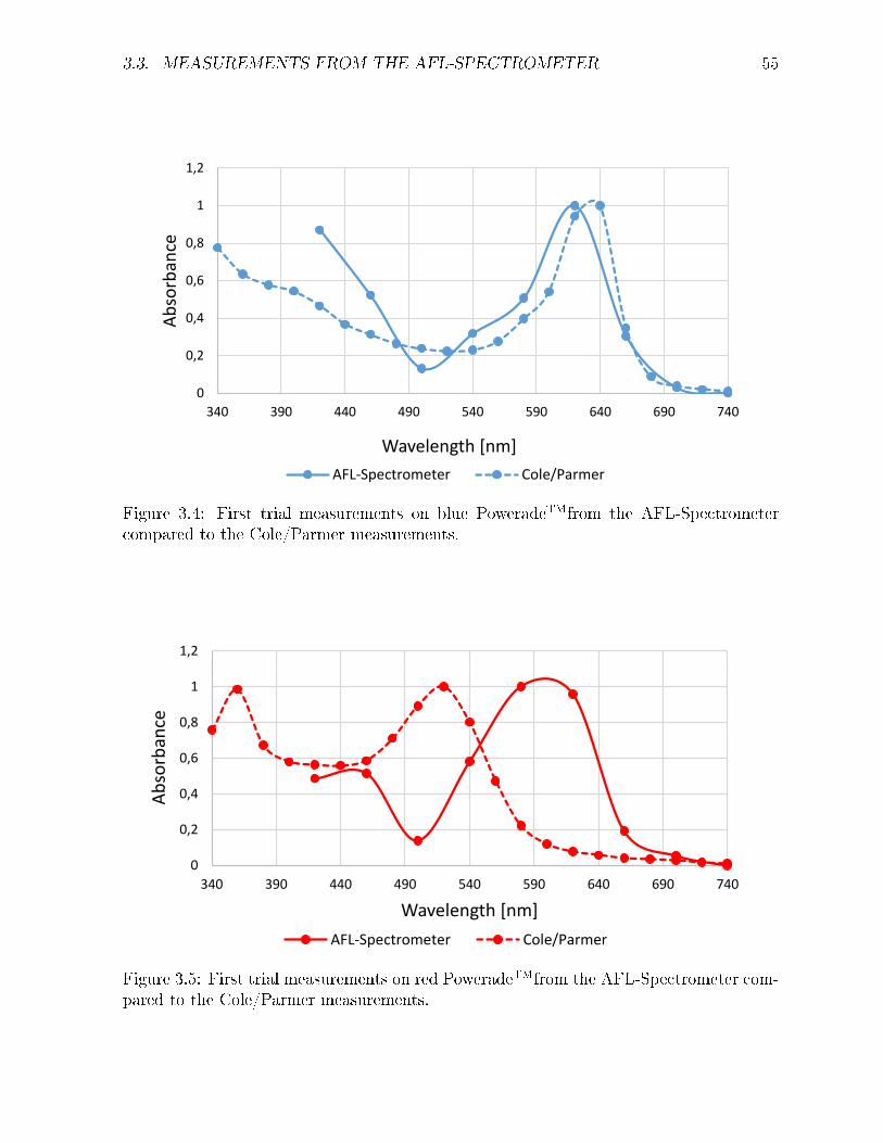
3.3. MEASUREMENTS FROM THE AFL-SPECTROMETER 55
0
0,2
0,4
0,6
0,8
1
1,2
340 390 440 490 540 590 640 690 740
Ab
sorb
ance
WavelengthL[nm]
AFL-Spectrometer Cole/Parmer
Figure 3.4: First trial measurements on blue PoweradeTMfrom the AFL-Spectrometercompared to the Cole/Parmer measurements.
0
0,2
0,4
0,6
0,8
1
1,2
340 390 440 490 540 590 640 690 740
Ab
sorb
ance
WavelengthL[nm]
AFL-Spectrometer Cole/Parmer
Figure 3.5: First trial measurements on red PoweradeTMfrom the AFL-Spectrometer com-pared to the Cole/Parmer measurements.

56 CHAPTER 3. RESULTS
0
0,2
0,4
0,6
0,8
1
1,2
340 390 440 490 540 590 640 690 740
Ab
sorp
tio
n
WavelengthF[nm]
AFL-Spectrometer Cole/Parmer
Figure 3.6: Second measurements made on the AFL-Spectrometer for bluePoweradeTM compared to the Cole/Parmer measurements. Amplied/ltered signal.
the noise was a very high percentage of the overall dierence between the signals (typicaldierence between the blank and the readout was between 5-20). The noise was thoughtto be having to big of an impact on these measurements to draw conclusions from them,but they still looked promising.
To test the device further, the signal from the TAOS sensor was amplied and lteredas has been described in the text, and second set of measurements was made. Filtrationeliminated a lot of the oscillation from the readout of the signal, moving the oscillationfrom the 10 down to ickering on about 2− 3. Amplication also helped utilize the A/Dconverter further, improving the resolution and minimizing the eect of the noise on eachreadout. Five sets of measurements were made and the average of those ve measurementswas plotted. Results can be seen in Figure 3.6 and 3.7.
Measurements plotted in Figures 3.6 and 3.7 were in an agreement with what hadalready been plotted in Figures 3.4 and 3.5 even though they were not identical, andshould thus have been reassuring. This caused concern. Flipping through the raw datafrom the measurements, it was evident that amplifying the signal did not increase thedierence between the readout of the samples and the blanks by the same factor as theamplication. Peaks of the wavelengths were also shifted to the sides, the blue peak wasshowing up on a lower wavelength than expected and the red peak was showing up at atoo high of a wavelength. Graphs were also being made by plotting the dierence betweenthe readout of the "blank" and the readout of the actual solution, and not by calculatingthe transmittance and turning it into absorption as Equations 1.2 and 1.3 describe. Eventhough this was eectively the dierence in light passing through the water and the

3.3. MEASUREMENTS FROM THE AFL-SPECTROMETER 57
0
0,2
0,4
0,6
0,8
1
1,2
340 390 440 490 540 590 640 690 740
Ab
sorp
tio
n
WavelengthF[nm]
AFL-Spectrometer Cole/Parmer
Figure 3.7: Second measurements made on the AFL-Spectrometer for redPoweradeTM compared to the Cole/Parmer measurements. Amplied/ltered signal.
sample, it did not seem quite right. To try to gure out what could be causing all of theconcerning factors just described, a third set of measurements was carried out this timeincluding a measurement for the LED without any sample being present. This had notbeen done in the previous two sets. Results from the third set of measurement can beseen in Figure 3.8
This is where the problems became evident. It was discovered that the LED beingused was not the RL5-W6030 diode that was thought to be in the device (which spectrawas introduced in Figure 2.12b). This was realized when the blank spectra was comparedto the reference. Secondly the measurements being made of the sports drinks were just aslightly less intense measurements of the blank spectra (by a very small amount) as canbe seen in the Figure. The LED that was in use was an RL5-WW7035 which spectracan be seen in Figure 3.10. This white LED spectra combined with the very nonlinearresponse of the TAOS sensor made measurements that was mistaken for noisy, slightlyshifted measurements comparable to the reference spectra made on the commercial units.This is evident when looking at Figure 3.10 and the response of the sensor side by side(the sensor response is shown in Figure 2.10a. WW7035 has two peaks, one that islocated directly between the peak of the red Powerade and the blue Powerade (580 nm vs520 nm and 630 nm), so when plotting the graphs individually it looked like these were twodistinct peaks showing up. When the measurements are examined more carefully, it getsevident that the peaks are in fact, the same peak. This became blatantly obvious whenthe "peaks" were plotted in the same graph for the rst time as is done in Figure 3.9.This peak is also located in the "sweet spot" of the sensor response curve.

58 CHAPTER 3. RESULTS
0
100
200
300
400
500
600
700
800
900
1000
380 430 480 530 580 630 680 730
A/D
BCo
nve
rter
Brea
do
ut
WavelengthB[nm]
Blank Red Blue
Figure 3.8: Measurement without a sample compared to Powerade reading.
0
0,2
0,4
0,6
0,8
1
1,2
360 410 460 510 560 610 660 710 760
Inte
nsi
ty
Wavelengthr[nm]Redrspectra Bluerspectra
Figure 3.9: Peaks of the red spectra and the blue spectra compared.

3.3. MEASUREMENTS FROM THE AFL-SPECTROMETER 59
Figure 3.10: Spectral response for the RL5-WW7035 LED [53].
Table 3.1: Readout for four concentrations of red food dye compared at 520nm.
Before grating After gratingBlank 191 191Water 190 140D1 187 85D2 184 52D3 183 11D4 179 7
What this also revealed was a aw in the concept of the device. As has been previouslydescribed, the sample was put in front of the diraction grating, as it was thought thatwavelengths would be equally absorbed in the sample independent of whether or not theyhad been broken up or not. This conclusion was wrong. To test this theory, a crudemeasurement was done using food dye to see how concentration would aect the sensoroutput, since it was known that measuring dierent concentrations at the peak wavelengthof a solution should result in a linear behaviour. A reference solution was prepared byputting a drop of food dye into water and it called dilution 1 (D1). Three other solutionswere then prepared, putting an additional drop of food dye in each one, two drops intoD2, three into D3 and four into D4 so that D4 had the darkest appearance and thereforethe highest concentration. These solutions were then measured, rst in the sampleholderof the device as it had been designed (before the diraction grating) and then immediatelyin front of the sensor (after the diraction grating) without being in a holder. Resultsfrom these measurements can be seen in Tables 3.1 to 3.4. Concentration graphs werealso plotted, as can be seen in Figures 3.11 and 3.12.
Tables 3.3 and 3.1 prove that the design concept was awed. Changes in concentrationbased on wavelength can not be performed with the sample in front of the diractiongrating. However at the peak intensity of each food dye solution the device can measurechanges in intensity just ne (peak concentrations of red and blue food dye are 520 and630 nm respectively [44]). A fairly linear relation is also realized in Figures 3.11 and 3.12supporting the claim even further.

60 CHAPTER 3. RESULTS
Table 3.2: Transmittance and Absorption for four concentrations of red food dye comparedat 520nm.
T AD1 0,52 0,65D2 0,32 1,14D3 0,07 2,70D4 0,04 3,15
Table 3.3: Readout for four concentrations of blue food dye compared at 630nm.
Before grating After gratingBlank 251 251Water 249 163D1 248 129D2 248 117D3 248 74D4 258 28
Table 3.4: Transmittance and Absorption for four concentrations of blue food dye com-pared at 630nm.
T AD1 0,79 0,23D2 0,72 0,33D3 0,45 0,79D4 0,17 1,76
0,00
0,50
1,00
1,50
2,00
2,50
3,00
3,50
0 1 2 3 4 5
Ab
sorp
tio
n
Dilution number
Figure 3.11: Concentration plot (Beer's graph) of red food dye.
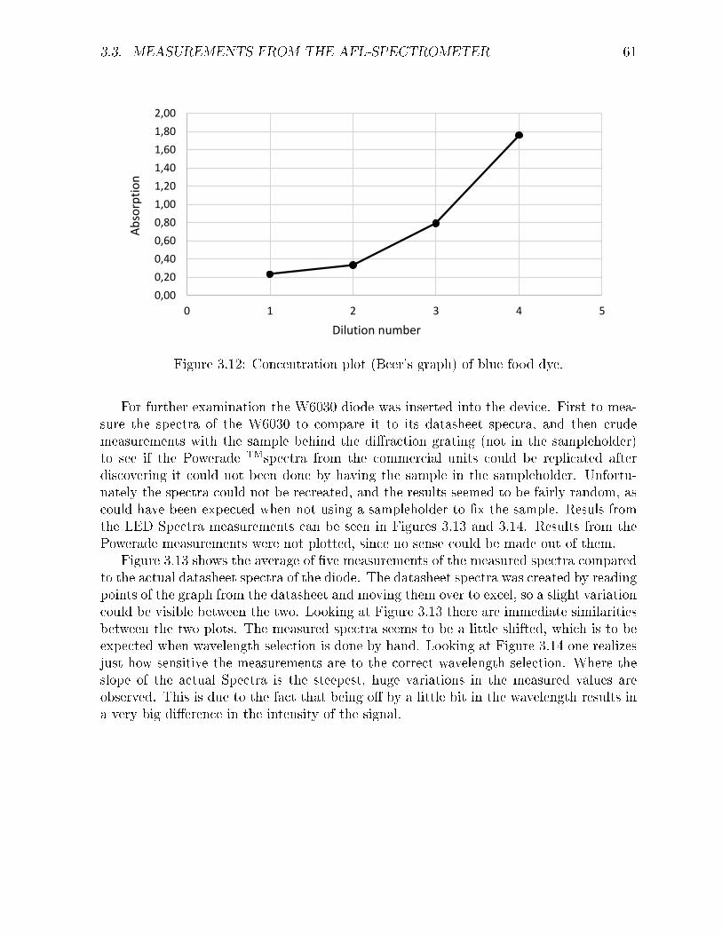
3.3. MEASUREMENTS FROM THE AFL-SPECTROMETER 61
0,00
0,20
0,40
0,60
0,80
1,00
1,20
1,40
1,60
1,80
2,00
0 1 2 3 4 5
Ab
sorp
tio
n
Dilution number
Figure 3.12: Concentration plot (Beer's graph) of blue food dye.
For further examination the W6030 diode was inserted into the device. First to mea-sure the spectra of the W6030 to compare it to its datasheet spectra, and then crudemeasurements with the sample behind the diraction grating (not in the sampleholder)to see if the Powerade TMspectra from the commercial units could be replicated afterdiscovering it could not been done by having the sample in the sampleholder. Unfortu-nately the spectra could not be recreated, and the results seemed to be fairly random, ascould have been expected when not using a sampleholder to x the sample. Resuls fromthe LED Spectra measurements can be seen in Figures 3.13 and 3.14. Results from thePowerade measurements were not plotted, since no sense could be made out of them.
Figure 3.13 shows the average of ve measurements of the measured spectra comparedto the actual datasheet spectra of the diode. The datasheet spectra was created by readingpoints of the graph from the datasheet and moving them over to excel, so a slight variationcould be visible between the two. Looking at Figure 3.13 there are immediate similaritiesbetween the two plots. The measured spectra seems to be a little shifted, which is to beexpected when wavelength selection is done by hand. Looking at Figure 3.14 one realizesjust how sensitive the measurements are to the correct wavelength selection. Where theslope of the actual Spectra is the steepest, huge variations in the measured values areobserved. This is due to the fact that being o by a little bit in the wavelength results ina very big dierence in the intensity of the signal.

62 CHAPTER 3. RESULTS
440 490 540 590 640 690 740
Average]Red
0,0
100,0
200,0
300,0
400,0
500,0
340 390 440 490 540 590
0,0
0,2
0,4
0,6
0,8
1,0
1,2
360 410 460 510 560 610 660 710 760
Inte
nsi
ty
Wavelengthm[nm]
MeasuredmLEDmspectra ActualmLEDmspectra
Figure 3.13: Measured LED Spectra compared to the datasheet Spectra.
90 740
0
200
400
600
800
1000
1200
360 410 460 510 560 610 660 710 760
Inte
nsi
ty
Wavelength [nm]
Figure 3.14: Five measurements of the LED spectra compared.

Chapter 4
Conclusion
Results from the thesis can, like mentioned before, be split up in two: reecting on thesuccess of the mechanical design on one hand, and the system as a measuring device onthe other.
It became clear that evaluation of the mechanical design would be very hard if nomeasurements had been made on the device. Measurements were made to try to replicatethe measurements made on the reference devices, which discovered a aw in the designconcept. Therefore no actual comparison could be made between the reference spectrameasured on the devices from HÍ and measurements from the AFL-Spectrometer. Thesemeasurements still served the purpose of leading to the discovery of the awed concept,and were thus very important.
Even though the mechanical design was impacted by the fact that the sampleholdershould have been on the other side of the diraction grating, the device fullled all themechanical design requirements set up in the axiomatic design framework. To every FRthere was a DP satisfying it, and therefore the design was completed in a satisfactorymanner from an axiomatic standpoint since no measurement constraints were on theproblem as it was dened. By misunderstanding the concept, the project was wronglydened in the beginning but the wrong denition was still correctly carried out in thephysical domain.
Even though full spectra of solutions cannot be measured by the device as is, it canstill serve its educational purpose. It can measure the spectra of a light source, and basedon measurements those light source spectrum could be produced very accurately withimprovements to wavelength selection. It can also be used to conduct experiments onBeer's law and thus serve students in both chemistry and physics. The only standardmeasurement it cannot produce that is the absorption spectra of a solution. Pendingconrmation, this could be xed by moving the already designed sampleholder behind thediraction grating, all three types of measurements would then be possible on the device.This would involve a redesign of the sampleholder and its position inside the device, sincethe sample would have to rotate to always be parallel to the sensor assembly.
The axiomatic design framework as a design foundation helped the designer discoveraws in the stage of zigzagging down the domains, realizing errors in the early stages of thedesign when cheap and easy to x. That being said, it did not help in discovering a aw in

64 CHAPTER 4. CONCLUSION
the concept, which conrms that a design can never be better than the understanding ofthe designer, and just as good as the functional requirements he chooses in the beginning.
What has been designed and realised can serve as a strong foundation, and with a littlemore work this could be a very rigorous, extremely aordable measuring device usable forall sorts of physics and chemistry experiments in the undergraduate laboratory setting.
4.1 Future work
Moving the AFL-Spectrometer further involves doing some work on it. First o, thesampleholder has to be moved to be behind the diraction grating in the optical pathof the device. A selection of wavelength has to be performed before the light is shonethrough the sample to be able to produce an absorption spectra for materials. Automatedwavelength selection is next in line to be implemented, to improve measurements for lightspectra and to make it possible to produce accurate absorption spectra. Finally the designmust be made freely available to interested parties, making a bundled solution from itwould also be an interesting task, since that would allow everybody in the proximity to aFab Lab to make their own UV-Vis spectrometer and start measuring.

Appendix A
Acclaro matrix
Printout from Acclaro DFSS

66 APPENDIX A. ACCLARO MATRIX
FR
6XGM
ea
sure
Gab
sorp
tion
GasGlig
htGp
asse
sGthro
ug
hGsa
mp
leGm
ate
rial
FR
NXGS
up
plyGp
ow
erGto
Gcom
po
ne
nts
FR
NDN
XGSu
pp
lyGpo
we
rGtoGlig
hts
FR
ND7
XGSu
pp
lyGpo
we
rGtoGC
PU
FR
NDE
XGSu
pp
lyGpo
we
rGtoGm
oto
rD
FR
7XGG
en
era
teGe
lectro
ma
gn
eticGra
dia
tion
Gon
Gvisible
Gspe
ctrum
FR
7DN
XGPro
vide
Gvwh
itevGlig
ht
FR
7D7
XGPro
vide
Gcalib
ratio
nGp
ea
ksGatGth
ree
Gkno
wn
Gwa
vele
ng
thsGo
fGthe
Gspe
ctra
FR
7DE
XGAcco
mp
an
yGou
tside
Gligh
tGsou
rce
FR
7DL
XGTra
nsfo
rmGlig
htGto
GaGp
oin
tGsou
rce
FR
EXGC
ollim
ate
Gligh
tGfrom
Gsou
rceD
FR
EDN
XGCo
llima
teGlig
htD
FR
ED7
XGAlig
nGco
llima
torGw
ithGlig
htGp
ath
Gaxia
lly
FR
EDE
XGSe
tGdista
nce
Gbe
twe
en
Gcollim
ato
rGan
dGlig
htGso
urce
D
FR
LXGP
assGlig
htGth
rou
gh
Gcon
stan
tGsam
ple
Gma
teria
lGthickn
ess
FR
LDN
XGKe
ep
Glen
gtGo
fGligh
tGpa
thGth
rou
gh
Gsam
ple
Gcon
stan
tGTaxia
lGcon
strain
txD
FR
LD7
XGKe
ep
Gsam
ple
GatGa
Gfixed
Gdista
nce
Gfrom
Gcollim
ato
rGlen
sGTcarte
sian
Gcon
strain
txD
FR
HXGS
plitGlig
htGin
toGm
ea
sura
ble
Gord
ere
dGsp
ectra
FR
HDN
XGDiffra
ctGcollim
ate
dGlig
htGa
tGan
Gan
gle
FR
HD7
XGFo
cusGfirstGo
rde
rGspe
ctraGo
nto
GaGp
lan
eGa
tGaGd
istan
ce
FR
BXGM
ea
sure
Gligh
tGinte
nsity
FR
BDN
XGSe
lectGw
ave
len
gth
FR
BDN
DNXGS
etGd
esire
dGw
ave
len
gtGva
lue
D
FR
BDN
D7XGC
on
trolGm
ove
me
ntGo
fGmo
tor
FR
BDN
DEXGM
ove
Gcen
terGo
fGligh
tGsen
sorGto
Gsele
cted
Gwa
vele
ng
th
FR
BDN
DLXGP
roh
ibitGm
ove
me
ntGo
fGmo
torGo
utsid
eGo
fGde
sired
Gran
ge
D
FR
BD7
XGNa
rrow
Gligth
Grea
chin
gGse
nso
rGfrom
Gspe
ctraGto
Gba
nd
FR
BDE
XGMe
asu
reGin
ten
sity
FR
BDL
XGPro
cessGd
ata
D
FR
BDL
DNXGC
on
vertGa
na
log
Gsen
sorGsig
na
lGvalu
eGto
Gdisp
laya
ble
Ginte
nsityD
FR
WXGP
rese
ntGd
ata
D
FR
WDN
XGDisp
layGd
ata
DP6XG Spectrometer
DPNXGElectonicGcircuit
DPNDNXGLEDGPowe
DPND7XGCPUGPowe
DPNDEXGMotorGpow
DP7XGLightGsource
DP7DNXGSuperbrigh
DP7D7XGThreeGcolo
DP7DEXGHoleGopen
DP7DLXGNarrowGslit
DPEXG CollimatingG lens
DPEDNXGBiconvexGle
DPED7XGLensGbrack
DPEDEXGSlitsGonGsp
DPLXG SampleG holding
DPLDNXGSampleGho
DPLD7XGMountingGh
DPHXG DiffractionG gratin
DPHDNXGDiffraction
DPHD7XG FocusingG
DPBXG LightG sensingG a
DPBDNXGWavelengt
DPBDNDNXGRotar
DPBDND7XGMotor
DPBDNDEXGStepp
DPBDNDLXGEndGs
DPBD7XGSheetGwith
DPBDEXGTAOSGTSL
DPBDLXGArduinoGUn
DPBDLDNXGArdui
DPWXG DisplayG assemb
DPWDNXGLiquidGCrys
X
XO
OO
OO
OO
OO
OO
OO
OO
OO
OO
OO
OO
OO
OO
XO
OO
OO
OO
OO
OO
OO
OO
OO
OO
OO
OO
OO
OO
OO
OX
OO
OO
OO
OO
OO
OO
OO
OO
OO
OO
OO
OO
OO
OO
OO
XO
OO
OO
OO
OO
OO
OO
OO
OO
OO
OO
OO
OO
OO
XX
OO
XO
OO
OO
OO
OO
OO
OO
OO
OO
OO
OO
O
XX
OO
XO
OO
OO
OO
OO
OO
OO
OO
OO
OO
OO
OO
OO
XX
OO
OX
OO
OO
OO
OO
OO
OO
OO
OO
OO
OO
OO
OO
OO
OO
OO
XO
OO
OO
OO
OO
OO
OO
OO
OO
OO
OO
OO
OO
OO
OO
OX
OO
OO
OO
OO
OO
OO
OO
OO
OO
OO
OO
OO
OO
OO
OO
OX
OO
OO
OO
OO
OO
OO
OO
OO
OO
OO
OO
OO
OO
OX
OO
OO
OO
OO
OO
OO
OO
OO
OO
OO
OO
OO
OO
OO
OO
XO
OO
OO
OO
OO
OO
OO
OO
OO
OO
OO
OO
OO
OO
OO
OX
OO
OO
OO
OO
OO
OO
OO
OO
OO
OO
OO
OO
OO
OO
OO
OX
OO
OO
OO
OO
OO
OO
OO
O
OO
OO
OO
OO
OO
OO
OX
OO
OO
OO
OO
OO
OO
OO
OO
OO
OO
OO
OO
OO
OO
OX
XO
OO
OO
OO
OO
OO
OO
OO
OO
OO
OO
OO
XX
XX
XO
OO
XO
OO
OO
OO
OO
OO
O
OO
OO
OO
OO
XX
XX
XO
OO
XO
OO
OO
OO
OO
OO
OO
OO
OO
OO
OO
XX
XX
XO
OO
XX
OO
OO
OO
OO
OO
OO
XO
XX
OO
OO
OO
OO
OO
OO
OO
OX
OO
XO
XX
OO
OO
XX
XX
XO
OO
XX
XX
OO
OO
OO
XO
XX
OO
OO
XX
XX
XO
OO
XX
XX
OO
OO
OO
OO
O
XO
XX
OO
OO
OO
OO
OO
OO
OO
OO
XO
OO
OO
OO
O
XO
XX
OO
OO
XX
XX
XO
OO
XX
XO
XX
OO
OO
OO
O
XO
XX
OO
OO
OO
OO
OO
OO
OO
OO
XX
XO
OO
OO
O
OO
OO
OO
OO
XX
XX
XO
OO
XX
XX
OO
OO
XO
OO
OO
OO
OO
OO
OO
OO
OO
OO
OO
OO
OO
OO
OO
OX
OO
OO
XO
XO
OO
OO
OO
OO
OO
OO
OO
OX
OO
OO
OO
XO
O
XO
XO
OO
OO
OO
OO
OO
OO
OO
OX
OO
OO
OX
XO
O
XO
XO
OO
OO
OO
OO
OO
OO
OO
OO
XO
OO
OO
OX
XX
XO
XO
OO
OO
OO
OO
OO
OO
OO
OO
XO
OO
OO
OX
XX

Appendix B
Bill of materials
Bill of materials for the nished spectrometer can be seen in Table B.1.
Table B.1: Bill of materials.
Item SupplierQuan-tity
Unit cost[$]
Total cost[$]
38mm Biconvex lens - f 150mm Ajax Scientc 3 6 18
Lens bracket Fab Lab Reykjavík 2 2 4
Arduino Uno Adafruit 1 24.95 24.95
Nema 17 Stepper motor Adafruit 1 14 14
Stepper Driver Pololu 1 5.95 5.95
MDF Local hardware store 2 6 12
Fasteners Local hardware store x x 50
LCD Adafruit 1 9.95 9.95
Rotary encoder Adafruit 1 4.5 4.5
Misc. electronic parts Adafruit 1 35 35
Diraction grating* Amazon 1 9.99 9.99
PEHD material Local hardware store 1 25 25
12V PSU 1000mA Local hardware store 1 30 30
Grand total 243.3

68

Bibliography
[1] J. E. Girard and C. T. Diamant, Instrumental analysis lecture and laboratory: asurvey, Journal of Chemical Education, vol. 77, no. 5, pp. 646648, 2000. [Online].Available: http://search.proquest.com/docview/211976097?accountid=28419.
[2] D. A. C. Czegan and D. K. Hoover, Uvvisible spectrometers: versatile instrumentsacross the chemistry curriculum, Journal of Chemical Education, vol. 89, no. 3,pp. 304309, 2012.
[3] J. R. Hamilton, J. S. White, and M. B. Nakhleh, Development of a low-cost four-color led photometer, Journal of Chemical Education, vol. 73, no. 11, p. 1052, 1996.
[4] Y. Kostov and G. Rao, Low-cost optical instrumentation for biomedical measure-ments, Review of Scientic Instruments, vol. 71, no. 12, pp. 43614374, 2000. [On-line]. Available: http://scitation.aip.org/content/aip/journal/rsi/71/12/10.1063/1.1319859.
[5] K. Knagge and D. Raftery, Construction and evaluation of a lego spectropho-tometer for student use, The Chemical Educator, vol. 7, no. 6, pp. 371375, 2002.[Online]. Available: http://dx.doi.org/10.1007/s00897020615a.
[6] D. R. Albert, M. A. Todt, and H. F. Davis, A low-cost quantitative absorptionspectrophotometer, Journal of Chemical Education, vol. 89, no. 11, pp. 14321435,2012.
[7] K. M. Cantrell and J. D. Ingle, The slim spectrometer, Analytical Chemistry, vol.75, no. 1, pp. 2735, 2003.
[8] P. C. Hauser and T. W. T. Rupasinghe, Simultaneous determination of metal ionconcentrations in binary mixtures with a multi-led photometer, Fresenius' Journalof Analytical Chemistry, vol. 357, no. 8, pp. 10561060, 1997. [Online]. Available:http://dx.doi.org/10.1007/s002160050304.
[9] Fab Foundation, What is a Fab Lab?, Cambridge, Massachusetts, USA, 2015. [On-line]. Available: http://www.fabfoundation.org/fab-labs/what-is-a-fab-lab/.
[10] P. Bernazzani and F. Paquin, Modular spectrometers in the undergraduate chem-istry laboratory, Journal of Chemical Education, vol. 78, no. 6, p. 796, 2001.
[11] A. Þór Stefánsson, E. A. Steinarsdóttir, G. H. Björnsson, M. Stefánsson, M. Ólaf-sson, and Ólöf K. Hrafnsdóttir, Spectroscope, T-865-MADE Precision Machine De-sign Final Report, 2011. [Online]. Available: http://afs.rnd.ru.is/course/T-865-MADE/2011/Projects/Spectrometer/Documentation/Report/report.pdf.

70 BIBLIOGRAPHY
[12] W. G. Schrenk, Historical development of ame excitation sources for analyticalspectroscopy, Applied Spectroscopy, 1986.
[13] J. Fraunhofer. [Online]. Available: http://www.aip.org/history/cosmology/tools/pic-spectroscopy-fraunhofer-spectrum.htm.
[14] S. I. Newton, Opticks or, a Treatise of the Reections, Refractions, Inections, andColours of Light. London : Printed for William Innys at the West-End of St. Paul's,1704.
[15] D. A. Skoog, D. M. West, F. J. Holler, and S. R. Crouch, Fundamentals of AnalyticalChemistry, 9th Edition, C. Simpson, Ed. Mary Finch, 2014.
[16] , Fundamentals of Analytical Chemistry, 9th Edition, C. Simpson, Ed. MaryFinch, 2014, pp. 651.
[17] Young and Freedman, University Physics with Modern Physics, P. Adam Black, Ed.Pearson/Addison Wesley, 2004.
[18] http://licht montage.com/. [Online]. Available: http : / / licht - montage . com/wp -content/uploads/2013/10/Visible-spectrum.png.
[19] T. Owen, Fundamentals of UV-visible spectroscopy. Primer, 2000.
[20] D. A. Skoog, D. M. West, F. J. Holler, and S. R. Crouch, Fundamentals of AnalyticalChemistry, 9th Edition, C. Simpson, Ed. Mary Finch, 2014, pp. 664.
[21] Beverage Universe. [Online]. Available: http://beverageuniverse.com/images/20oz-Mt-Blast.gif.
[22] IDS Education. [Online]. Available: http : //www. inds . co .uk/howto/ food - dye -forensics.htm.
[23] D. A. Skoog, F. J. Holler, and S. R. Crouch, Principles of Instrumental Analysis,6th Edition, S. Kiselica, Ed. David Harris, 2007.
[24] The Vietnam Open Educational Resources. [Online]. Available: https://voer.edu.vn/le/53787.
[25] Wikimedia. [Online]. Available: http://upload.wikimedia.org/wikipedia/commons/thumb/8/86/Ebohr1-IP.svg/2000px-Ebohr1-IP.svg.png.
[26] The Vietnam Open Educational Resources. [Online]. Available: http://voer.edu.vn/c/multiple-slit-diraction/0e60bfc6/665e6e55.
[27] , [Online]. Available: http://voer.edu.vn/c/multiple-slit-diraction/0e60bfc6/665e6e55.
[28] T.-S. Yeh and S.-S. Tseng, A low cost led based spectrometer, Journal of theChinese Chemical Society, vol. 53, no. 5, pp. 10671072, 2006. [Online]. Available:http://dx.doi.org/10.1002/jccs.200600142.
[29] N. P. Suh, Axiomatic Design - Advances and Applications. Oxford University Press,2001.
[30] , Axiomatic design theory for systems, Research in engineering design, vol.10, no. 4, pp. 189209, 1998.

BIBLIOGRAPHY 71
[31] , Complexity. Oxford University Press, 2005.
[32] , Designing-in of quality through axiomatic design, Reliability, IEEE Trans-actions on, vol. 44, no. 2, pp. 256264, 1995.
[33] E. M. Benavides, Advanced engineering design - An integrated approach. WoodheadPublishing, 2012.
[34] M. K. Thompson, A classication of procedural errors in the denition of functionalrequirements in axiomatic design theory, 2013.
[35] N. P. Suh, The principles of Design. Oxford University Press, 1990, pp. 26.
[36] , The principles of Design. Oxford University Press, 1990.
[37] , Axiomatic Design - Advances and Applications. Oxford University Press, 2001,pp. 116.
[38] M. S. Hundal, Systematic Mechanical Design: a cost and management perspective.New York, NY: ASME Press, 1997.
[39] M. K. Thompson, Improving the requirements process in axiomatic design theory,CIRP Annals-Manufacturing Technology, vol. 62, no. 1, pp. 115118, 2013.
[40] Wikipedia. [Online]. Available: http://en.wikipedia.org/wiki/Thin\-lens\#mediaviewer/File:Lens1.svg.
[41] M. O'Toole and D. Diamond, Absorbance based light emitting diode optical sensorsand sensing devices, Sensors, vol. 8, no. 4, pp. 24532479, 2008.
[42] P. K. Dasgupta, I.-Y. Eom, K. J. Morris, and J. Li, Light emitting diode-based de-tectors: absorbance, uorescence and spectroelectrochemical measurements in a pla-nar ow-through cell, Analytica Chimica Acta, vol. 500, pp. 337364, 2003. [Online].Available: http://www.sciencedirect.com/science/article/pii/S0003267003005750.
[43] , Light emitting diode-based detectors: absorbance, uorescence and spectro-electrochemical measurements in a planar ow-through cell, Analytica ChimicaActa, 2003. [Online]. Available: http ://www.sciencedirect . com/science/article/pii/S0003267003005750.
[44] Royal Society of Chemistry, Food dye analysis. [Online]. Available: http://www.rsc.org/learn-chemistry/resource/download/res00000941/cmp00000328/pdf.
[45] Fab Lab BCN. [Online]. Available: http :// fablabbcn.org/wp- content/uploads/2013/01/makerbot-replicator2.jpg.
[46] Epilog. [Online]. Available: http://www.epiloglaser.co.uk/assets/img/products/helix24-model.jpg.
[47] N. Narendran and Y. Gu, Life of led-based white light sources, Display Technology,Journal of, vol. 1, no. 1, pp. 167171, 2005.
[48] AMS ag. [Online]. Available: http://ams.com/eng/Products/Light-Sensors/Light-to-Voltage-Sensors/TSL257.
[49] Arduino. [Online]. Available: http://arduino.cc/en/Main/ArduinoBoardUno.

72 BIBLIOGRAPHY
[50] , [Online]. Available: http://store.arduino.cc/bmz-cache/4/4578f41d9764a5c236470019f05dd2bc.image.447x354.jpg.
[51] Amber Spyglass. [Online]. Available: http://store.amberspyglass .co.uk/images/source/Electronics/NEMA17-1.8deg-40mm-stepper-motor.jpg.
[52] Bar-Naor. [Online]. Available: http : //www.barnaor . com/ images/NewsImages/cuvettes.jpg.
[53] Superbrightleds. [Online]. Available: https://www.superbrightleds.com/moreinfo/through-hole/5mm-warm-white-led-35-degree-viewing-angle-7000-mcd/264/1191/#/tab/Specications.

Glossary
AFL-Spectrometer A spectrometer designed to be manufacturable aordable and man-ufacturable in a Fab Lab, the subject of this thesis. 15, 21, 22, 24, 28, 29, 31, 32,35, 36, 41, 42, 45, 52, 54, 63, 64
Fab Lab A Fabrication Laboratory (Fab Lab for short) is a workshop that oers studentsand other interested parties the opportunity to digitally fabricate their designs atminimum cost. xxiv, 1, 17, 3032, 44, 64
LEGO Plastic construction toys made by LEGO in Denmark. LEGO consists of plasticbricks that can be interlocked together in a relatively repeatable manner. 1
MADE-Spectrometer A spectrometer built in the graduate level course T-865-MADEunder the supervision of Joseph Foley in 2011. This device served as a model/inspi-ration for the AFL-Spectrometer. 2, 15, 16, 22, 26, 27, 34, 35, 41, 42
Spectra A rainbow of color produced when white light is shined through a prism or adiraction grating sheet. 35, 8, 15, 16, 2427, 32, 3537, 40, 41, 61
stepper motor A stepper motor is a DC motor that rotates in a stepwise manner asopposed to the normal conitinious motion of regular DC motors. stepper motorscane be precisely moved to a desired location without a feedback mechanism.. 15,34, 35, 40, 73
T-865-MADE Precision Machine Design - a graduate level course focusing on teachinghow to design and manufacture machines where precision is of big importance. T-865-MADE is the identication number used in the RU for the course.. 2

74
Acronyms
ABS Acrylonitrile butadiene styrene. 31
CAD Computer-aided Design. xxiv, 14, 15, 36, 37, 39, 41
CNs Customer Needs/Customer Attributes. 12, 17, 21, 22, 32
Cs Constraints. 17
DPs Design Parameters. 1214, 16, 17, 21, 22, 47
FRs Functional Requirements. 1214, 1618, 21, 22, 45, 47
LCD Liquid crystal display. 14, 15, 18, 42
LED Light-emitting diode. xxiv, 1, 16, 2426, 28, 3033, 36, 47, 48, 51, 57, 61
MDF Medium-density berboard. 28, 29, 31, 3537, 40, 41, 44, 45
PCB Printed circuit board. 15, 41, 42
PEHD High-density polyethylene. 35, 40
PLA Polylactic Acid. 31, 32
PMMA Plexiglas. 31
PVs Process Variables. 12, 21
RGB Red Green Blue. 16, 28, 32, 33
UV-Vis Ultraviolet-visible. 1, 8

76

ACRONYMS 77

78

School of Science and EngineeringReykjavík UniversityMenntavegur 1101 Reykjavík, IcelandTel.+354 599 6200Fax +354 599 6201www.ru.is