Embed Size (px)
Citation preview

FLORIDA STATE UNIVERSITY
FAMU–FSU COLLEGE OF ENGINEERING
LOW-COST CONCENTRATING SOLAR COLLECTOR FOR STEAM
GENERATION
By
JOHN DASCOMB
A Thesis submitted to theDepartment of Mechanical Engineering
in partial fulfillment of therequirements for the degree of
Master of Science
Degree Awarded:Spring Semester, 2009

The members of the Committee approve the Thesis of John Dascomb defended on March
26, 2009.
Anjaneyulu KrothapalliProfessor Directing Thesis
Brenton GreskaCommittee Member
Juan Carlos OrdonezCommittee Member
William S. OatesCommittee Member
The Graduate School has verified and approved the above named committee members.
ii

TABLE OF CONTENTS
List of Tables . . . . . . . . . . . . . . . . . . . . . . . . . . . . . . . . . . . . . . v
List of Figures . . . . . . . . . . . . . . . . . . . . . . . . . . . . . . . . . . . . . vi
Abstract . . . . . . . . . . . . . . . . . . . . . . . . . . . . . . . . . . . . . . . . ix
1. INTRODUCTION . . . . . . . . . . . . . . . . . . . . . . . . . . . . . . . . . 11.1 Motivation . . . . . . . . . . . . . . . . . . . . . . . . . . . . . . . . . . 11.2 Literature Review . . . . . . . . . . . . . . . . . . . . . . . . . . . . . . . 31.3 Previous Work . . . . . . . . . . . . . . . . . . . . . . . . . . . . . . . . 91.4 Project Goal . . . . . . . . . . . . . . . . . . . . . . . . . . . . . . . . . 11
2. BACKGROUND . . . . . . . . . . . . . . . . . . . . . . . . . . . . . . . . . . 132.1 Introduction to the Solar Spectrum . . . . . . . . . . . . . . . . . . . . . 132.2 Solar Geometry . . . . . . . . . . . . . . . . . . . . . . . . . . . . . . . . 142.3 Optics . . . . . . . . . . . . . . . . . . . . . . . . . . . . . . . . . . . . . 232.4 Receiver Design . . . . . . . . . . . . . . . . . . . . . . . . . . . . . . . . 282.5 Steam Boiler Design . . . . . . . . . . . . . . . . . . . . . . . . . . . . . 34
3. EXPERIMENTAL SETUP . . . . . . . . . . . . . . . . . . . . . . . . . . . . 393.1 Parabolic Dish . . . . . . . . . . . . . . . . . . . . . . . . . . . . . . . . 393.2 Reflective Surface . . . . . . . . . . . . . . . . . . . . . . . . . . . . . . . 413.3 Frame . . . . . . . . . . . . . . . . . . . . . . . . . . . . . . . . . . . . . 423.4 Receiver . . . . . . . . . . . . . . . . . . . . . . . . . . . . . . . . . . . . 443.5 Tracking . . . . . . . . . . . . . . . . . . . . . . . . . . . . . . . . . . . . 463.6 Data Acquisition and Instrumentation . . . . . . . . . . . . . . . . . . . 47
4. RESULTS AND DISCUSSION . . . . . . . . . . . . . . . . . . . . . . . . . . 504.1 Thermal Efficiency Results . . . . . . . . . . . . . . . . . . . . . . . . . . 504.2 System Characterization . . . . . . . . . . . . . . . . . . . . . . . . . . . 584.3 Optical Efficiency . . . . . . . . . . . . . . . . . . . . . . . . . . . . . . . 634.4 Boiler Efficiency . . . . . . . . . . . . . . . . . . . . . . . . . . . . . . . 634.5 Insulation Efficiency . . . . . . . . . . . . . . . . . . . . . . . . . . . . . 634.6 Error . . . . . . . . . . . . . . . . . . . . . . . . . . . . . . . . . . . . . . 644.7 Cost Analysis . . . . . . . . . . . . . . . . . . . . . . . . . . . . . . . . . 64
iii
5. CONCLUSION . . . . . . . . . . . . . . . . . . . . . . . . . . . . . . . . . . . 675.1 Future Work . . . . . . . . . . . . . . . . . . . . . . . . . . . . . . . . . 68
APPENDICES . . . . . . . . . . . . . . . . . . . . . . . . . . . . . . . . . . . . . 69
A. RECEIVER DRAWINGS . . . . . . . . . . . . . . . . . . . . . . . . . . . . . 69
B. CONNECTION ARM DRAWINGS . . . . . . . . . . . . . . . . . . . . . . . 74
C. CONCENTRATOR CONNECTION RING DRAWINGS . . . . . . . . . . . . 77
D. FOUNDATION DRAWINGS . . . . . . . . . . . . . . . . . . . . . . . . . . . 80
REFERENCES . . . . . . . . . . . . . . . . . . . . . . . . . . . . . . . . . . . . . 83
BIOGRAPHICAL SKETCH . . . . . . . . . . . . . . . . . . . . . . . . . . . . . 85
iv

LIST OF TABLES
4.1 Average Values for Testing Performed Feb 23, 2009 . . . . . . . . . . . . . . 59
4.2 Optical Efficiency . . . . . . . . . . . . . . . . . . . . . . . . . . . . . . . . . 63
4.3 Absorber Efficiency . . . . . . . . . . . . . . . . . . . . . . . . . . . . . . . . 64
4.4 Material Costs . . . . . . . . . . . . . . . . . . . . . . . . . . . . . . . . . . . 66
v

LIST OF FIGURES
1.1 World HDI vs. Electricity Consumption [1] . . . . . . . . . . . . . . . . . . . 1
1.2 Pifre’s 1878 Sun-Power Plant Driving a Printing Press [2] . . . . . . . . . . . 3
1.3 Boing/SES DECC Dish Stirling System [3] . . . . . . . . . . . . . . . . . . . 4
1.4 Process Flow and Corresponding Thermodynamic State for Shenandoah TotalEnergy Project [4] . . . . . . . . . . . . . . . . . . . . . . . . . . . . . . . . 6
1.5 Process Flow and Thermodynamic State for Johnson and Johnson SolarFacility [4] . . . . . . . . . . . . . . . . . . . . . . . . . . . . . . . . . . . . . 7
1.6 Overall View of Solar 1, at Barstow, CA [4] . . . . . . . . . . . . . . . . . . 8
1.7 Solar Configuration of INDITEP Project Seville, Spain [6] . . . . . . . . . . 8
1.8 Schematic of Solar 1 . . . . . . . . . . . . . . . . . . . . . . . . . . . . . . . 9
1.9 Concentrator Assembly for Solar 1 [8] . . . . . . . . . . . . . . . . . . . . . . 10
1.10 Receiver Assembly for Solar 1 [8] . . . . . . . . . . . . . . . . . . . . . . . . 11
2.1 Solar Spectrum at the Surface of the Earth . . . . . . . . . . . . . . . . . . . 14
2.2 Average Insolation for Tallahassee [7] . . . . . . . . . . . . . . . . . . . . . . 15
2.3 Declination Angle at Summer Solstice[8] . . . . . . . . . . . . . . . . . . . . 16
2.4 Declination Angle Versus Day of Year [9] . . . . . . . . . . . . . . . . . . . . 17
2.5 Sidereal Time Shift [5] . . . . . . . . . . . . . . . . . . . . . . . . . . . . . . 17
2.6 Shift in Solar Time . . . . . . . . . . . . . . . . . . . . . . . . . . . . . . . . 18
2.7 Analemma (Yearly Solar Shift) . . . . . . . . . . . . . . . . . . . . . . . . . 18
2.8 Horizontal Coordinate System [18] . . . . . . . . . . . . . . . . . . . . . . . . 20
2.9 Altitude Angle vs. Time of Day for Tallahassee, Florida . . . . . . . . . . . . 20
vi

2.10 Azimuth Angle vs. Time of Day for Tallahassee, Florida . . . . . . . . . . . 21
2.11 Alt-Azimuth Mount . . . . . . . . . . . . . . . . . . . . . . . . . . . . . . . . 22
2.12 Solar Concentrator with an Equatorial Mount System [2] . . . . . . . . . . . 23
2.13 Receiver Temp. vs. Concentration Ratio . . . . . . . . . . . . . . . . . . . . 24
2.14 Specular Reflectance . . . . . . . . . . . . . . . . . . . . . . . . . . . . . . . 25
2.15 Ray tracing on a parabola . . . . . . . . . . . . . . . . . . . . . . . . . . . . 26
2.16 Intercept factor vs. Aperture Diameter for Typical Dish . . . . . . . . . . . . 28
2.17 Cavity Receiver [8] . . . . . . . . . . . . . . . . . . . . . . . . . . . . . . . . 30
2.18 Radiant Flux of a Blackbody [2] . . . . . . . . . . . . . . . . . . . . . . . . . 32
2.19 Convection Loss vs. Tilt Angle for Open and Covered Cavities . . . . . . . . 35
2.20 Water Tube Boiler [11] . . . . . . . . . . . . . . . . . . . . . . . . . . . . . . 36
2.21 Typical Boiling Curve [10] . . . . . . . . . . . . . . . . . . . . . . . . . . . . 37
3.1 Bare Concentrator Wedge . . . . . . . . . . . . . . . . . . . . . . . . . . . . 40
3.2 Fully Assembled Concentrator . . . . . . . . . . . . . . . . . . . . . . . . . . 41
3.3 Mounting Frame . . . . . . . . . . . . . . . . . . . . . . . . . . . . . . . . . 42
3.4 Receiver Assembly and Connection Ring . . . . . . . . . . . . . . . . . . . . 43
3.5 Energy Absorption vs. Aperture Diameter . . . . . . . . . . . . . . . . . . . 45
3.6 Exploded View of Receiver . . . . . . . . . . . . . . . . . . . . . . . . . . . . 45
3.7 Assembled Receiver . . . . . . . . . . . . . . . . . . . . . . . . . . . . . . . . 46
3.8 Assembled Linear Actuators . . . . . . . . . . . . . . . . . . . . . . . . . . . 47
3.9 Dual Axis Tracking Sensor . . . . . . . . . . . . . . . . . . . . . . . . . . . . 48
3.10 Schematic of Test Setup . . . . . . . . . . . . . . . . . . . . . . . . . . . . . 49
3.11 Eppley Nominal Incidence Pyrheliometer . . . . . . . . . . . . . . . . . . . . 49
4.1 Testing Performed Feb 23, 2009 . . . . . . . . . . . . . . . . . . . . . . . . . 51
4.2 Testing Performed March 02, 2009 . . . . . . . . . . . . . . . . . . . . . . . . 51
4.3 Testing Performed March 04, 2009 . . . . . . . . . . . . . . . . . . . . . . . . 52
vii

4.4 Superheated Steam Production March 09, 2009 . . . . . . . . . . . . . . . . 53
4.5 Testing Performed March 02, 2009 Display of Salt Bath Phase Change . . . 54
4.6 Testing Performed Sept 04, 2008 0.7 LPM . . . . . . . . . . . . . . . . . . . 55
4.7 Testing Performed February 24, 2009 1.0 LPM . . . . . . . . . . . . . . . . . 56
4.8 Testing Performed Feb 22, 2009 1.5 LPM . . . . . . . . . . . . . . . . . . . . 57
4.9 Testing Performed Feb 19, 2009 1.3 LPM . . . . . . . . . . . . . . . . . . . . 57
4.10 Testing Performed February 26, 2009 1.1 LPM . . . . . . . . . . . . . . . . . 58
4.11 Intercept Factor for Solar 2 . . . . . . . . . . . . . . . . . . . . . . . . . . . 60
4.12 Distribution of Thermal Losses . . . . . . . . . . . . . . . . . . . . . . . . . 62
viii

ABSTRACT
Concentrating solar power (CSP) is a unique renewable energy technology. CSP
systems have the ability to provide electricity, refrigeration and water purification in one
unit. This technology will be extremely helpful in improving the quality of life for many
people around the world who lack the energy needed to live a healthy life.
An economic parabolic dish concentrating system was built at the Sustainable Energy
Science and Engineering Center (SESEC) at Florida State University in Tallahassee, Florida.
The goal of the project was to provide 6.67 kW of thermal energy. This is the amount of
energy required to produce 1 kW of electricity with a conventional micro steam turbine. The
system had a price goal of $1000 per kW and must be simple enough to be maintained by
non-technical personnel. A 14 m2 fiberglass parabolic concentrator was made at SESEC to
ensure simplicity of production and operation. The concentrator was coated with a highly
reflective polymer film. The cavity type receiver was filled with sodium nitrate to act as a
heat storage and transfer medium. The collection efficiency of the cavity was estimated at
70%. The gross thermal conversion efficiency of the system was 39%, which represented a
333% improvement over the first concentrator assembled at SESEC. At peak insolation 5.46
kW of thermal energy was produced. The material cost for the system was $3,052.
ix

CHAPTER 1
INTRODUCTION
1.1 Motivation
The world is dependent upon energy. People’s energy use directly correlates to their grade
of health care, life expectancy and education. These are important factors that determine a
person’s quality of life. One quantitative measure of life quality is the Human Development
Index (HDI). The HDI combines life expectancy, literacy, education and GDP per capita for
different countries. Figure 1.1 displays the HDI versus electricity use for different countries
and one can see the clear correlation between electricity consumption and HDI.
Electricity allows people access to refrigeration for food and medicine, energy for cooking
Figure 1.1: World HDI vs. Electricity Consumption [1]
1
and cleaning water, and allows people to read and study at night when there is little work
that can be done outside. A small amount of electricity can dramatically change the life of
a person who has had none. It is estimated that the power requirement for basic healthy
functioning in rural communities is about 0.08 kWh/day/person [12]. This is less than 1%
of an average person’s usage in the United States, yet many people can not afford or do not
have access to even this small amount.
Nearly two billion people live in rural areas without access to electrical grids. Developing
an infrastructure in these remote areas is usually not feasible due to the extreme distance
from existing electric grids. Building new power plants in these areas is not cost effective
due to the relatively low electricity consumption. Economical, small-scale, distributed energy
systems can fulfill the need and renewable energy is ideally suited for this purpose.
Many under-developed areas around the world receive large amounts of sunlight. North-
ern Africa and Central Asia receive as much as 7.5 kWh/m2/day. There is great opportunity
to use solar power to provide basic energy needs in these regions. The two most prominent
solar energy technologies are photovoltaic (PV) and concentrated solar power (CSP). PV
systems are beneficial because they can be scaled to any size, but they are costly and
solely produce electricity. CSP systems can provide electricity as well as thermal power.
This thermal power can be efficiently used for cooking, water distillation and absorption
refrigeration cycles. The drawback to these systems is that the most efficient solar thermal
systems currently have an installation cost of $10,000/kW [13]. An economic CSP system
could provide rural areas with electricity and energy needs to dramatically improve their
quality of life.
This project is a continuation of work performed at the Sustainable Energy Science and
Engineering Center (SESEC) to build an economic CSP system. The first system built at
SESEC constantly provided roughly 2.5 kW of thermal energy. 6.67 kW is the minimum
input power required for a micro-steam turbine to produce 1 kW of electrical power. The
goal of this project is to provide at least 6.67 kW of thermal power at an installation cost of
$1,000. The system must be easy enough to be constructed and maintained by non-technical
personnel.
2

1.2 Literature Review
1.2.1 Brief History of Solar Thermal Power
Concentrating solar power is a method of increasing solar power density. Using a
magnifying glass to set a piece of paper on fire demonstrates the basic principle of CSP.
Sunlight shining on the curved glass is concentrated to a small point. When all the heat
energy that was spread across the surface of the magnifying glass is focused to a single point,
the result is a dramatic rise in temperature. The paper will reach temperatures above 451
◦F and combust. CSP has been theorized and contemplated by inventors for thousands of
years. It is possible that as far back as ancient Mesopotamia, priestesses used polished golden
vessels to ignite altar fires. The first documented use of concentrated power comes from
the great Greek scientist Archimedes (287-212 B.C.). Stories of Archimedes repelling the
invading Roman fleet of Marcellus in 212 B.C. by burning their ships with concentrated solar
rays were told by Galen (A.D. 130-220) [2]. In the seventeenth century, Athanasius Kircher
(1601-1680) set fire to a woodpile at a distance in order to prove the story of Archimedes
[2]. This is considered the beginning of modern solar concentration. Solar concentrators
then began being used as furnaces in chemical and metallurgical experiments [14]. They
were preferred because of the high temperatures they could reach without the need for any
fuel. Further applications opened for concentrated power when August Mouchot pioneered
Figure 1.2: Pifre’s 1878 Sun-Power Plant Driving a Printing Press [2]
generating low-pressure steam to operate steam engines between 1864 and 1878. Abel Pifre
made one of his solar engines operate a printing press in 1878 at the Paris Exhibition [2],
3

Figure 1.3: Boing/SES DECC Dish Stirling System [3]
but after extensive testing he declared the system too expensive to be feasible. His press
is shown in Figure 1.2. Pifre’s and Mouchot’s research began a burst of growth for solar
concentrators.
The early twentieth century brought many new concentrating projects varying from solar
pumps to steam power generators to water distillation. A 50 kW solar pump made by
Shuman and Boys in 1912 was used to pump irrigation water from the Nile. Mirrored
troughs were used in a 1200 m2 collector field to provide the needed steam [15]. In 1920 J.A.
Harrington used a solar-powered steam engine to pump water up 5 m into a raised tank.
This was the first documented use of solar storage. The water was stored for continual use as
power for a turbine inside a small mine [15]. Concentrating technology had made a huge leap
from the nineteenth century but was halted by World War II and the resulting explosion of
cheap fossil fuels. The advantages of solar power lost their luster and the technology would
merely inch forward for nearly five decades.
Starting in the late seventies and early eighties, solar power came back to the forefront
of researchers’ agendas with oil and gas shortages. In 1977 in Shenandoah, GA, 114 7-meter
parabolic dishes were used to heat a silicon-based fluid for a steam Rankine cycle. The plant
also supplied waste heat to a lithium bromide absorption chiller. The plants total thermal
efficiency was 44%, making it one of the most efficient systems ever implemented [4]. More
modern systems like the Department of Energy’s Dish Engine Critical Components (DECC)
project, which was built at the National Solar Thermal Test Facility, consisted of a 89 m2
dish with a peak system electrical efficiency of 29.4% [3]. This system utilizes the high
4

efficiency of the sterling engine to convert the heat generated into electricity. This efficiency
is unmatched by any concentrator that utilizes a steam cycle, with one or two working fluids.
1.2.2 Solar Steam Generation
Solar thermal systems can utilize the Rankine cycle to produce electricity. This is done
by creating steam using solar energy and passing it through a turbine. The most common
modern technique to produce steam for electricity production or industrial needs has been
to utilize a heat transfer fluid. Usually a salt or oil is pumped through a solar field to heat
up the fluid. The hot oil is then passed through a heat exchanger with water to generate
steam. The benefit of a heat transfer fluid is that it remains liquid at high temperatures,
which increases heat transfer and ease of pumping. Oils have a liquid working range up to
400 ◦C, salts up to 600 ◦C and liquid metals can reach much higher temperatures.
The Solar Total Energy Project in Shenandoah, Georgia used a heat transfer fluid to
create electricity and process steam for a textile factory. The heat transfer fluid used was
Syltherm 800, a silicon-based fluid produced by Dow-Corning Corporation. The Syltherm
carried 2.6 MW of heat from 114 7 m diameter concentrating parabolic dishes. The fluid was
pumped to cavity receivers that were placed at the focal point of each dish. The collector
efficiency of the concentrators was 76.9%. Three heat exchangers were then utilized to
preheat, boil and superheat water before it was passed through a steam turbine. A portion
of the steam generated was used directly by the factory. The remaining hot water was used
as a heat sink for a lithium bromide absorption chiller. The electricity generation efficiency
was 11.8%. The total heat work efficiency for all of the processes was 44.6% [4]. Figure 1.4
shows the process flow and corresponding state for the system.
Even though using an oil or salt as a heat transfer fluid is the most popular choice,
water is still used in some cases. The Johnson and Johnson Solar Process Heat System
used pressurized water as the heat transfer fluid in a parabolic trough plant. The facility
had 1070 m2 of parabolic troughs which heated water pressurized at 310 psi to 200 ◦C.
The water was stored in a tank where flash steam was created 4 times a day for industrial
processes. To create steam, the pressurized water was throttled down to 125 psi where it
vaporized additional feed water. The saturated steam that was produced was sent to do
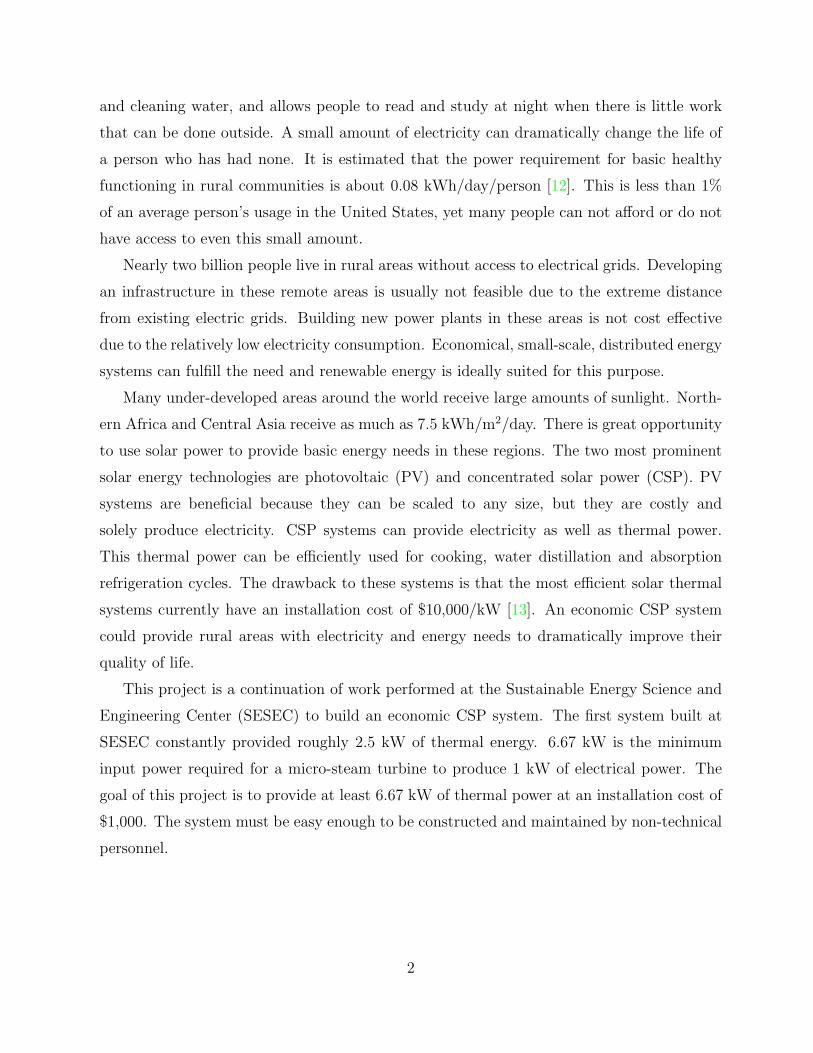
work. Thermal collection efficiency for the system was 30% [4]. Figure 1.5 shows the process
flow and corresponding thermodynamic state for this facility.
5

Figure 1.4: Process Flow and Corresponding Thermodynamic State for Shenandoah TotalEnergy Project [4]
6
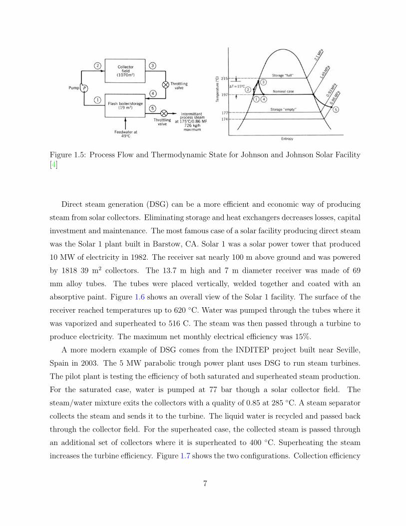
Figure 1.5: Process Flow and Thermodynamic State for Johnson and Johnson Solar Facility[4]
Direct steam generation (DSG) can be a more efficient and economic way of producing
steam from solar collectors. Eliminating storage and heat exchangers decreases losses, capital
investment and maintenance. The most famous case of a solar facility producing direct steam
was the Solar 1 plant built in Barstow, CA. Solar 1 was a solar power tower that produced
10 MW of electricity in 1982. The receiver sat nearly 100 m above ground and was powered
by 1818 39 m2 collectors. The 13.7 m high and 7 m diameter receiver was made of 69
mm alloy tubes. The tubes were placed vertically, welded together and coated with an
absorptive paint. Figure 1.6 shows an overall view of the Solar 1 facility. The surface of the
receiver reached temperatures up to 620 ◦C. Water was pumped through the tubes where it
was vaporized and superheated to 516 C. The steam was then passed through a turbine to
produce electricity. The maximum net monthly electrical efficiency was 15%.
A more modern example of DSG comes from the INDITEP project built near Seville,
Spain in 2003. The 5 MW parabolic trough power plant uses DSG to run steam turbines.
The pilot plant is testing the efficiency of both saturated and superheated steam production.
For the saturated case, water is pumped at 77 bar though a solar collector field. The
steam/water mixture exits the collectors with a quality of 0.85 at 285 ◦C. A steam separator
collects the steam and sends it to the turbine. The liquid water is recycled and passed back
through the collector field. For the superheated case, the collected steam is passed through
an additional set of collectors where it is superheated to 400 ◦C. Superheating the steam
increases the turbine efficiency. Figure 1.7 shows the two configurations. Collection efficiency
7
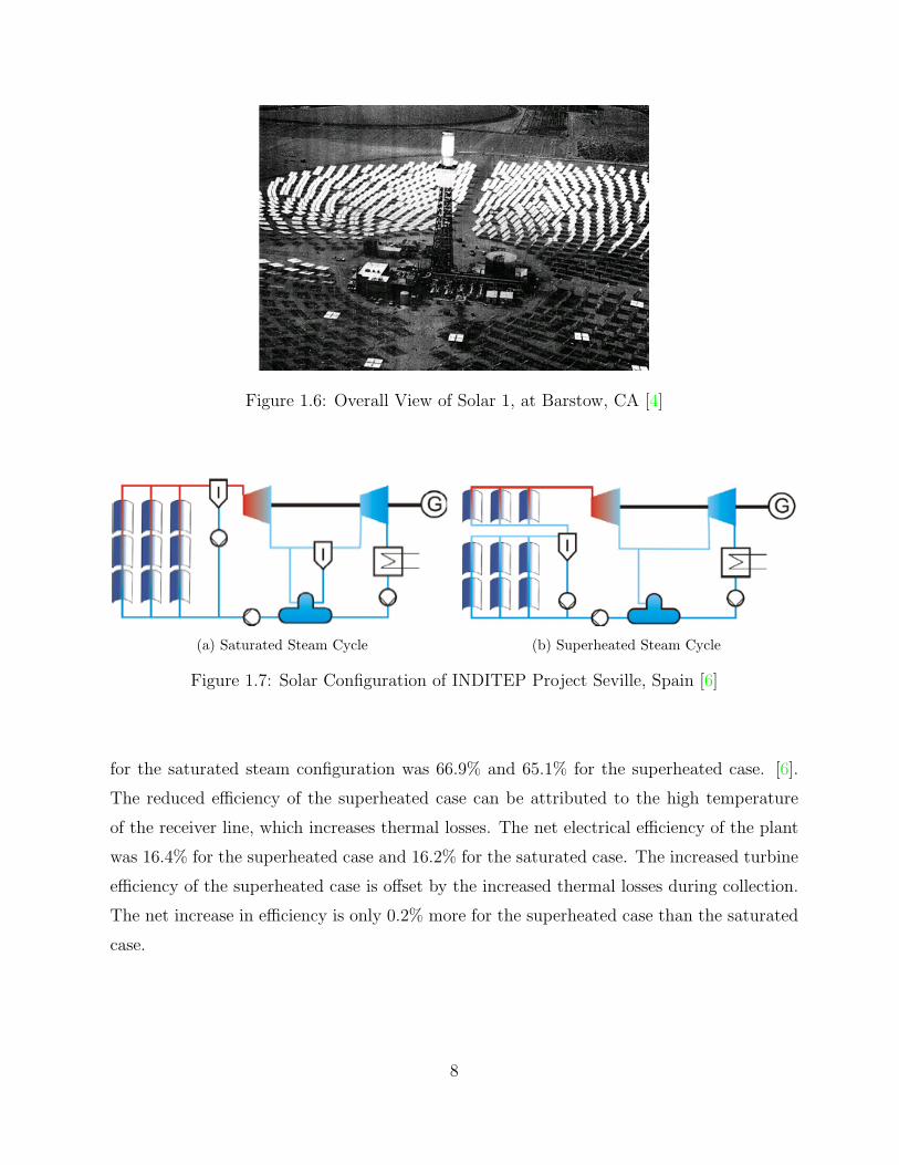
Figure 1.6: Overall View of Solar 1, at Barstow, CA [4]
(a) Saturated Steam Cycle (b) Superheated Steam Cycle
Figure 1.7: Solar Configuration of INDITEP Project Seville, Spain [6]
for the saturated steam configuration was 66.9% and 65.1% for the superheated case. [6].
The reduced efficiency of the superheated case can be attributed to the high temperature
of the receiver line, which increases thermal losses. The net electrical efficiency of the plant
was 16.4% for the superheated case and 16.2% for the saturated case. The increased turbine
efficiency of the superheated case is offset by the increased thermal losses during collection.
The net increase in efficiency is only 0.2% more for the superheated case than the saturated
case.
8

Figure 1.8: Schematic of Solar 1
1.3 Previous Work
An economic solar dish system was built in 2006 by graduate student C. Christopher
Newton. This first dish system built at SESEC , nicknamed Solar 1, attempted to complete
the same goal as the one addressed in this paper, which is to provide 1 kW of electrical
energy for an installation cost of only $1000 dollars. Figure 1.8 shows a schematic of the
the system. A parabolic concentrator reflected solar radiation to a central receiver. The
receiver produced intermittent steam that was injected into a steam turbine. The turbine
was connected to an electric generator that produced electricity.
The concentrator used was a fiberglass Channel Master satellite dish with an aperture
diameter of 3.66 m. Figure 1.9 shows the operational concentrator. Solar 1 pivoted on a
steel alt-azimuth type frame. Two independent linear actuators move the dish throughout
the day. The actuators were controlled automatically by a set of photo-sensing modules.
The modules consisted of light sensing LEDs that sent signals to the actuators when the
module was not oriented normal to incoming solar radiation. The power for the sensors and
actuators was provided by 2 small thin film photovoltaic panels, which charged two 24 V
deep cell batteries. The reflective material used to coat the fiberglass surface was aluminized
mylar, which has an optical reflectivity of 76%.
The system utilized an external type receiver that had an absorber diameter of 15 cm.
9

Figure 1.9: Concentrator Assembly for Solar 1 [8]
The absorber was coated with a high temperature black paint, which has an absorptivity
and emissivity both equal to 90%. The receiver was filled with draw salt to act as a heat
storage and heat transfer medium. Draw salt is a 1:1 molar ratio of potassium nitrate and
sodium nitrate. The melting temperature of this eutectic mixture is 223 ◦C.
The heat exchanger in the receiver consisted of an abbreviated water tube boiler, which
consisted of copper tubes coiled around the outer rim of the salt bath. They connected to a
water drum in contact with the flat absorber at the base of the receiver. The steam in the
water drum exited through copper tubes in the center of the receiver. Figure 1.10 shows the
Solar 1 receiver assembly.
The maximum steady state thermal output for the system was 1 kW. The resulting
thermal conversion efficiency was estimated at 9.03%. To produce electricity, water was
held in the receiver where it pressurized and released in intervals at a 6.67% duty cycle.
The maximum electrical conversion efficiency was estimated at 1.94%, which equated to a
turbine efficiency near 15%. The maximum gross electricity production by Solar 1 was 220
W.
The majority of the thermal losses for Solar 1 are believed to be from three major factors.
First, the concentrator efficiency was extremely poor. The reflected focal area was much
larger than the receiver. Much of the radiation was reflected onto the side of the receiver,
which was heavily insulated and thus lost. Second, the reflective material had incredibly poor
weathering abilities. In the few months before testing the surface was exposed to the elements
and pollution in the atmosphere. During final testing the mylar was visibly cloudy and
10

Figure 1.10: Receiver Assembly for Solar 1 [8]
turning yellow, clearly indicating a greatly reduced reflectivity. The last major factor hurting
system efficiency was the absorber. The flat plat absorber, although compact, was extremely
exposed and lost tons of energy to the environment through convection and radiation. This
type of receiver is extremely sensitive to wind, and the results show dramatic drops in receiver
temperature with any wind at all. These three factors are primarily responsible for the low
thermal conversion energy and must be improved in the second concentrator if it is to be
successful.
1.4 Project Goal
The first concentrator system built at SESEC, Solar 1, attempted to satisfy all of the
research objectives held by SESEC for this project. Mirror and boiler inefficiencies held
the system from producing enough steam to continuously run a micro-steam turbine. The
minimum thermal input to run a micro-steam turbine is near 5 kW, 5 times what was
produced by Solar 1. Furthermore, a micro-steam turbine with 15% thermal efficiency
requires 6.67 kW of thermal energy to produce 1 kW of electricity. For the project discussed
in this thesis, it was decided to focus only on the thermal energy generation and neglect
electrical generation. Once enough thermal energy is being produced, a micro-steam turbine
11

will then by implemented. The goal of this project is to rebuild the concentrator and receiver
assembly to produce 6.67 kW of thermal energy for an installation cost of $1000 dollars.
12
CHAPTER 2
BACKGROUND
2.1 Introduction to the Solar Spectrum
The Sun is an enormous atomic reactor, constantly fusing hydrogen nuclei together to
form helium. In the process it gives off huge amounts of energy in the form of electromagnetic
radiation. This radiated energy can travel infinite distances to nearby planets, such as Earth,
or planets millions of light years away. The Sun emits 4×1026 W of energy and only 1.7×10¹⁷
W reaches the Earth [14]. The Earth receives less than one billionth of the Sun’s power
output.
Electromagnetic (EM) radiation is a self propagating wave that carries energy through
space. EM radiation is classified into types according to the frequency of the wave. At
less than 1 pm, gamma rays encompass the smallest wavelengths of EM radiation. Radio
waves have the longest wavelengths and start at 1 mm. In between these two limits there
are classifications such as microwaves, terahertz, infrared, visible, ultraviolet and X-rays.
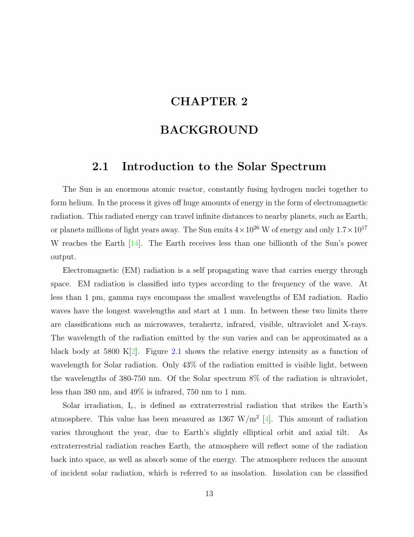
The wavelength of the radiation emitted by the sun varies and can be approximated as a
black body at 5800 K[2]. Figure 2.1 shows the relative energy intensity as a function of
wavelength for Solar radiation. Only 43% of the radiation emitted is visible light, between
the wavelengths of 380-750 nm. Of the Solar spectrum 8% of the radiation is ultraviolet,
less than 380 nm, and 49% is infrared, 750 nm to 1 mm.
Solar irradiation, Ir, is defined as extraterrestrial radiation that strikes the Earth’s
atmosphere. This value has been measured as 1367 W/m2 [4]. This amount of radiation
varies throughout the year, due to Earth’s slightly elliptical orbit and axial tilt. As
extraterrestrial radiation reaches Earth, the atmosphere will reflect some of the radiation
back into space, as well as absorb some of the energy. The atmosphere reduces the amount
of incident solar radiation, which is referred to as insolation. Insolation can be classified
13

Figure 2.1: Solar Spectrum at the Surface of the Earth
into two types: direct normal insolation and diffuse insolation. Direct normal insolation
is the radiation that travels directly through the atmosphere without interference. Diffuse
insolation is scattered by particles in the atmosphere, eventually hitting the Earth at random
angles, an effect that can be observed on a cloudy day. For reasons which will be explained
below, this project deals exclusively with direct normal insolation. The average amount
of direct normal insolation throughout the day for Tallahassee can be seen in Figure 2.2
Between 09:00 and 17:00 the average is about 450 W/m2.
2.2 Solar Geometry
The Earth is rotating about the Sun in an elliptical orbit at a rate of 1 rotation every
365 + 1/4 days. The Earth is on average 1.5 × 10¹¹meters away from the Sun [18]. The
Earth’s axis of rotation is tilted at an angle of 23.45◦ with respect to its orbital plane. This
tilt causes the angle at which sunlight hits the Earth to change throughout the year. For the
months of June through September the northern hemisphere is tilted toward the Sun and
the Sun’s rays shine normal to the surface. In the winter months, the northern hemisphere
is tilted away from the Sun and sunlight hits the surface at lesser angles. As the incident sun
angle moves away from zenith angle (θ) equal to zero(directly overhead), sunlight is spread
14

Figure 2.2: Average Insolation for Tallahassee [7]
over a larger area and is less intense. This relationship is described in units of Air Mass
(AM). An Air Mass equal to 1 is when the Sun is directly overhead shining normal to the
surface, called zenith. Equation 2.1 gives the equation for Air Mass in terms of zenith angle
(θ) [18]. The equation is applicable for angles between 0◦ and 70◦. At a zenith angle of 60◦
the Air Mass is 2, which means incident radiation is half of what it is when the Sun is at
zenith.
AM =1
cos(θ)(2.1)
The position of the Sun changes considerably throughout the year. The different types
of solar motion are described in the following sections.
2.2.1 Diurnal Rotation
The first and most basic motion of the Sun is diurnal, or daily, rotation. The sun makes
an apparent pass around Earth every 24 hours, rotating around an axis called the celestial
axis. This axis differs at times from our magnetic axis by as much as 6◦. If an observer were
standing on the celestial equator during the equinox, the sun would pass directly overhead
going from East to West. If the observer were to line up a telescope on an axis pointed
directly at celestial north, the rotation of the telescope following the Sun would be 1◦ every
4 minutes, or 360◦ every day.
15
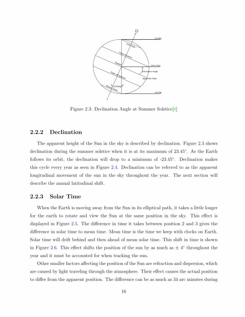
Figure 2.3: Declination Angle at Summer Solstice[8]
2.2.2 Declination
The apparent height of the Sun in the sky is described by declination. Figure 2.3 shows
declination during the summer solstice when it is at its maximum of 23.45◦. As the Earth
follows its orbit, the declination will drop to a minimum of -23.45◦. Declination makes
this cycle every year as seen in Figure 2.4. Declination can be referred to as the apparent
longitudinal movement of the sun in the sky throughout the year. The next section will
describe the annual latitudinal shift.
2.2.3 Solar Time
When the Earth is moving away from the Sun in its elliptical path, it takes a little longer
for the earth to rotate and view the Sun at the same position in the sky. This effect is
displayed in Figure 2.5. The difference in time it takes between position 2 and 3 gives the
difference in solar time to mean time. Mean time is the time we keep with clocks on Earth.
Solar time will drift behind and then ahead of mean solar time. This shift in time is shown
in Figure 2.6. This effect shifts the position of the sun by as much as ± 4◦ throughout the
year and it must be accounted for when tracking the sun.
Other smaller factors affecting the position of the Sun are refraction and dispersion, which
are caused by light traveling through the atmosphere. Their effect causes the actual position
to differ from the apparent position. The difference can be as much as 34 arc minutes during
16

Figure 2.4: Declination Angle Versus Day of Year [9]
Figure 2.5: Sidereal Time Shift [5]
sunrise and sunset, which is slightly larger than the viewed size of the sun.
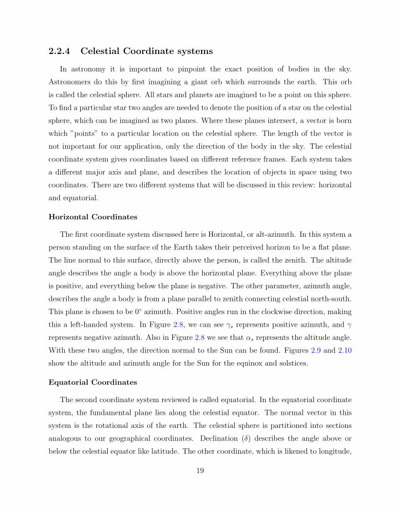
The net effect of the two major sources of solar shift can be seen in Figure 2.7. This
unsymmetrical figure 8 is referred to as an analemma. It shows the position of the Sun at
the same mean time every day of the year. There are 3 parameters that create this image.
The two greatest factors, declination and equation of time, have already been discussed. The
third parameter distorts the figure-8 from being symmetric horizontally and is caused by the
difference in angle between the apse line and the line of solstices.
17
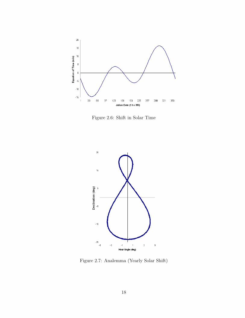
Figure 2.6: Shift in Solar Time
Figure 2.7: Analemma (Yearly Solar Shift)
18
2.2.4 Celestial Coordinate systems
In astronomy it is important to pinpoint the exact position of bodies in the sky.
Astronomers do this by first imagining a giant orb which surrounds the earth. This orb
is called the celestial sphere. All stars and planets are imagined to be a point on this sphere.
To find a particular star two angles are needed to denote the position of a star on the celestial
sphere, which can be imagined as two planes. Where these planes intersect, a vector is born
which ”points” to a particular location on the celestial sphere. The length of the vector is
not important for our application, only the direction of the body in the sky. The celestial
coordinate system gives coordinates based on different reference frames. Each system takes
a different major axis and plane, and describes the location of objects in space using two
coordinates. There are two different systems that will be discussed in this review: horizontal
and equatorial.
Horizontal Coordinates
The first coordinate system discussed here is Horizontal, or alt-azimuth. In this system a
person standing on the surface of the Earth takes their perceived horizon to be a flat plane.
The line normal to this surface, directly above the person, is called the zenith. The altitude
angle describes the angle a body is above the horizontal plane. Everything above the plane
is positive, and everything below the plane is negative. The other parameter, azimuth angle,
describes the angle a body is from a plane parallel to zenith connecting celestial north-south.
This plane is chosen to be 0◦ azimuth. Positive angles run in the clockwise direction, making
this a left-handed system. In Figure 2.8, we can see γs represents positive azimuth, and γ
represents negative azimuth. Also in Figure 2.8 we see that αs represents the altitude angle.
With these two angles, the direction normal to the Sun can be found. Figures 2.9 and 2.10
show the altitude and azimuth angle for the Sun for the equinox and solstices.
Equatorial Coordinates
The second coordinate system reviewed is called equatorial. In the equatorial coordinate
system, the fundamental plane lies along the celestial equator. The normal vector in this
system is the rotational axis of the earth. The celestial sphere is partitioned into sections
analogous to our geographical coordinates. Declination (δ) describes the angle above or
below the celestial equator like latitude. The other coordinate, which is likened to longitude,
19

Figure 2.8: Horizontal Coordinate System [18]
Figure 2.9: Altitude Angle vs. Time of Day for Tallahassee, Florida
20

Figure 2.10: Azimuth Angle vs. Time of Day for Tallahassee, Florida
is called hour angle (H). The hour angle uses units of hours, minutes, and seconds to partition
the 360◦ sphere into 24 hours. One hour angle equals 15◦ of arc. Following these coordinates
simplifies the apparent motion of the sun. The change in hour angle is constant throughout
the day at 1◦ every 4 minutes. The declination changes by no more than 4 tenths of a degree
per day.
To convert between the two coordinate systems we may use Equations 2.2 and 2.3. These
equations give altitude and azimuth angle for the sun given the observers latitude (Φ),
declination (δ) and hour angle (H) [16].
sinα = sinδ × sinΦ + cosδ × cosΦ× cosH (2.2)
cosγ × cosα = cosΦ× sinδ − sinΦ× cosδ × cosH (2.3)
Using Equations 2.2 and 2.3 we can easily plot the motion of the sun throughout the entire
year.
21
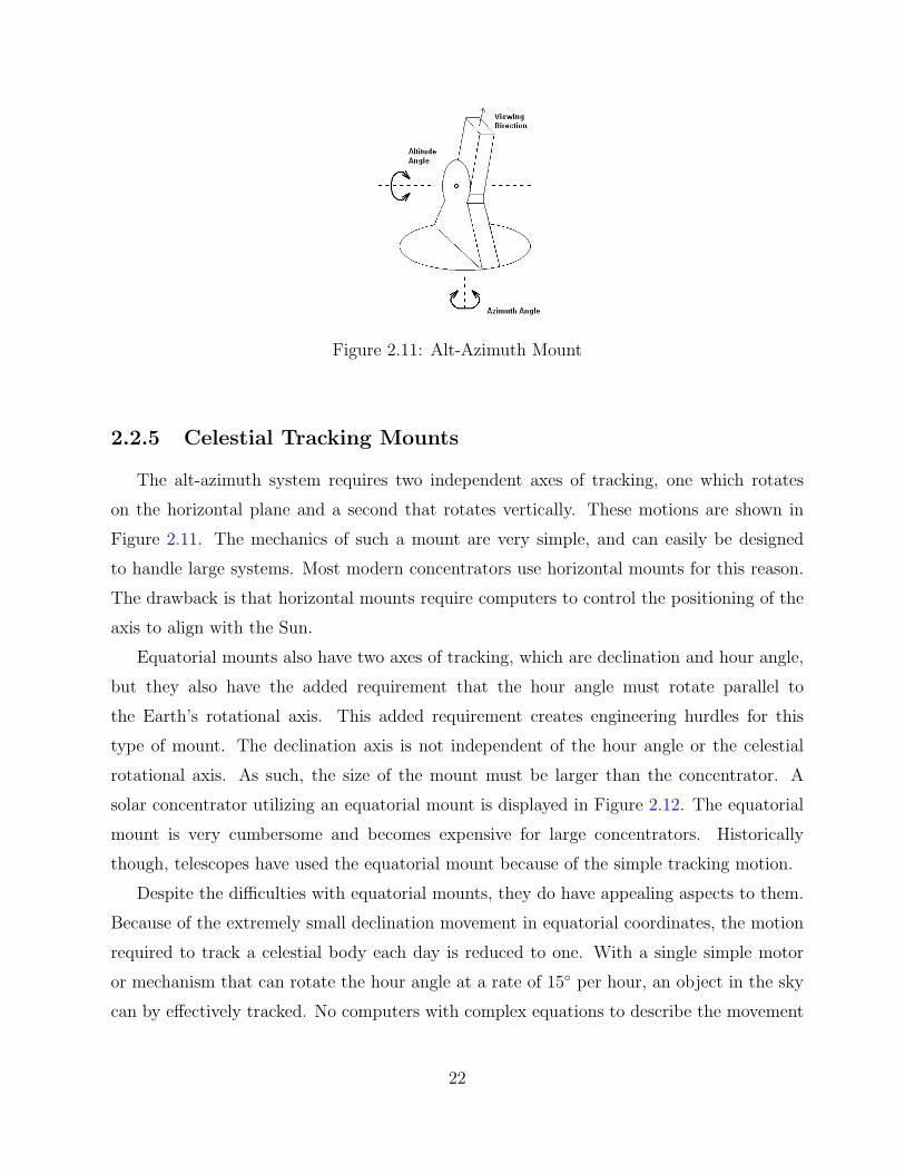
Figure 2.11: Alt-Azimuth Mount
2.2.5 Celestial Tracking Mounts
The alt-azimuth system requires two independent axes of tracking, one which rotates
on the horizontal plane and a second that rotates vertically. These motions are shown in
Figure 2.11. The mechanics of such a mount are very simple, and can easily be designed
to handle large systems. Most modern concentrators use horizontal mounts for this reason.
The drawback is that horizontal mounts require computers to control the positioning of the
axis to align with the Sun.
Equatorial mounts also have two axes of tracking, which are declination and hour angle,
but they also have the added requirement that the hour angle must rotate parallel to
the Earth’s rotational axis. This added requirement creates engineering hurdles for this
type of mount. The declination axis is not independent of the hour angle or the celestial
rotational axis. As such, the size of the mount must be larger than the concentrator. A
solar concentrator utilizing an equatorial mount is displayed in Figure 2.12. The equatorial
mount is very cumbersome and becomes expensive for large concentrators. Historically
though, telescopes have used the equatorial mount because of the simple tracking motion.
Despite the difficulties with equatorial mounts, they do have appealing aspects to them.
Because of the extremely small declination movement in equatorial coordinates, the motion
required to track a celestial body each day is reduced to one. With a single simple motor
or mechanism that can rotate the hour angle at a rate of 15◦ per hour, an object in the sky
can by effectively tracked. No computers with complex equations to describe the movement
22

Figure 2.12: Solar Concentrator with an Equatorial Mount System [2]
are necessary.
2.3 Optics
2.3.1 Concentration
The concentration ratio of a parabolic concentrator (PC) is given by Equation 2.4 [2].
Ac is the projected area of the concentrator, and Ar is the receiver area.
CR =AdAr
(2.4)
The maximum possible concentration ratio for a 3-D collector with a source half angle of θ
is given in Equation 2.5 [17].
CRmax =1
sin θ2(2.5)
For a concentrator using the Sun as its source, the half angle is approximately 1/4◦ [19].
This means the maximum concentration with a 3-D concentrator is approximately 5000.
The higher the concentration ratio, the higher the maximum temperature will be. Achieving
high temperatures is a unique characteristic to PCs. Ideally, the maximum temperature
achievable by a concentrator is the source temperature. Equation 2.6 gives the absorber
temperature Tabs for a PC neglecting conduction and convection.
Tabs = Ts[(1− η)× ηoptεabs× CR× sinθ2]1/4 (2.6)
23

Figure 2.13: Receiver Temp. vs. Concentration Ratio
given the following values:
TS = Temperature of the source (K)
η = Efficiency of transferring heat to working fluid
ηopt = Optical efficiency of concentrator system
εabs = Emissivity of absorber
The maximum temperature of a receiver versus concentration ratio is graphed in Figure 2.13
under usual concentrator conditions.
2.3.2 Reflection
The manipulation of light and other EM waves can be achieved in a number of ways; it
can reflect off of a surface, transmit through a material without effect, or be absorbed by
the surface. With absorption, the EM waves increase the energy of the impinging surface.
Equation 2.7 describes a particular surface depending upon it’s coefficient of reflectivity, ρ,
transmittance, τ , and absorptivity, γ. Each coefficient describes the relative effect the surface
has on the radiation that impinges upon it. For example a surface with τ = 1 would transmit
all radiation through the material and none would be reflected or absorbed. Coefficients of a
material change depending on radiation wavelength, surface temperature and incident angle.
24

Figure 2.14: Specular Reflectance
To simplify analysis, coefficients are averaged for regions of interest and given a single value.
ρ+ τ + γ = 1 (2.7)
There are two types of reflection; diffuse and specular. A diffuse surface reflects the light
rays in a number of different directions. Specular reflectors are “mirror” like and the angle
of incidence (θi) equals the angle of reflection (θr), as given by Snell’s law. For a specular
reflecting surface, a method called ray-tracing can accurately determine the path of reflected
EM waves. Ray tracing reduces a large field of particles traveling through a system to a
discrete number of narrow beams called rays. Solving the path of these rays accurately
predicts the movement of an entire field of particles. Figure 2.14 shows the path of light
striking a mirror for a specular reflecting surface.
A parabola is a curve generated by the intersection of a right circular cone and a plane
parallel to an element of the curve. Equation 2.8 describes a parabola that is symmetric
about the y-axis.
y = ax2 (2.8)
EM rays incoming parallel to the symmetric axis intersect at a single point called the focus
or focal point. This point is found by using Equation 2.9. Ray tracing on a parabola is
displayed in Figure 2.15. In this figure the rim angle, (φ), is defined as the incidence angle
of light striking the outer rim of the concentrator.
f =1
4a(2.9)
25

Figure 2.15: Ray tracing on a parabola
2.3.3 Optical Efficiency
An ideal concentrator focuses all light that hits its surface to a single point. In reality,
errors in the optics of the dish skew the light increasing the size of the focal beam. Total
angular error due to optics can be calculated using Equation 2.10 [7].
σtot =√
(2× σconc)2 + (σtracking)2 + (σrefl)2 + (σabs)2 + (σsun)2 (2.10)
where angular errors are due to:
σsun - suns rays not being perfectly parallel
σtracking - concentrator alignment with sun
σconc - concentrator surface irregularities
σrefl - non specular reflector
σabs - receiver alignment with focal point
By determining the total angular error in a concentrator we can accurately determine the
flux capture fraction, Γ. The flux capture fraction relates the percentage of light reflected
to a desired circular area at the focal point with diameter (d). Equation 2.11 gives the value
of the flux capture fraction.
Γ = 1− 2×Qx (2.11)
where:
Qx = fx × (b1 × t+ b2 × t2 + b3 × t3 + b4 × t4 + b5 × t5)
fx =1√
2× π× exp(−x
2
2)
26

t =1
(1 + r × x)
x = n/2
n = arctan(d× cos(φ)p
)× (2/σtot)
and:
r = .2316419
b1 = 0.379381530
b2 = −0.356563782
b3 = 1.781477937
b4 = −1.821255978
b5 = 1.330274429
d = Receiver diameter
φ = Rim angle
p = Distance from focal point to rim of the paraboloid
The standard angular error found in state of the art paraboloid concentrators, (σ), is 6.7
mrad [7]. This translates to an intercept factor of 1 at an aperture diameter of 4.8 in. This
means that 100% of the reflected radiation is focused to a circular area with a diameter of
4.8 in, centered at the focal point. As the total angular error increases it takes an increasing
aperture diameter to capture the same amount of radiation. Figure 2.16 shows the intercept
factor for differing aperture diameters.
The optical efficiency of a concentrator system (ηopt) describes a CPCs ability to reflect
and absorb solar radiation. The optical efficiency is the product of the reflection of radiation
off the reflective surface, ηrefl, and absorption of radiation to the receiver, ηabs. This efficiency
is shown in Equation 2.12.
ηopt = ηrefl × ηabs (2.12)
A perfect system would have a reflectivity coefficient for the concentrator equal to 1 and
an absorptivity coefficient for the absorber also equal to 1. Reflectors will always absorb
small amounts radiation and absorbers will reflect some radiation reducing the total system
efficiency.
27
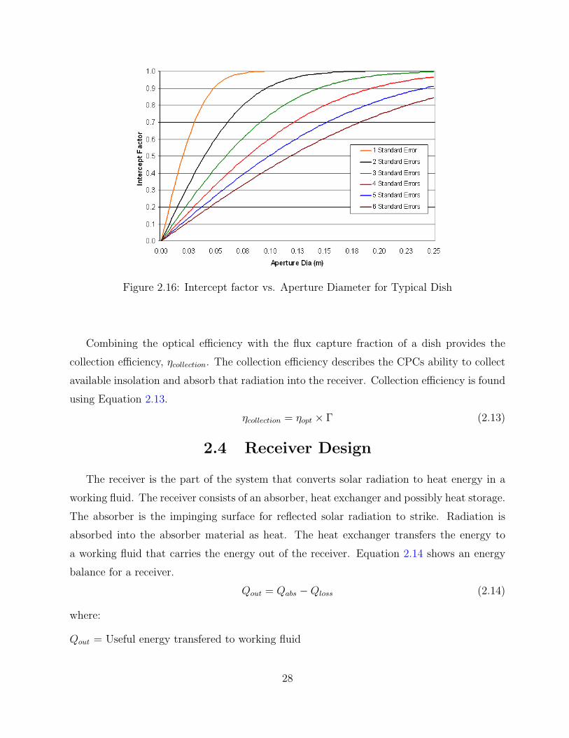
Figure 2.16: Intercept factor vs. Aperture Diameter for Typical Dish
Combining the optical efficiency with the flux capture fraction of a dish provides the
collection efficiency, ηcollection. The collection efficiency describes the CPCs ability to collect
available insolation and absorb that radiation into the receiver. Collection efficiency is found
using Equation 2.13.
ηcollection = ηopt × Γ (2.13)
2.4 Receiver Design
The receiver is the part of the system that converts solar radiation to heat energy in a
working fluid. The receiver consists of an absorber, heat exchanger and possibly heat storage.
The absorber is the impinging surface for reflected solar radiation to strike. Radiation is
absorbed into the absorber material as heat. The heat exchanger transfers the energy to
a working fluid that carries the energy out of the receiver. Equation 2.14 shows an energy
balance for a receiver.
Qout = Qabs −Qloss (2.14)
where:
Qout = Useful energy transfered to working fluid
28
Qabs = Energy collected by the absorber
Qloss = Receiver energy losses
and total receiver efficiency ηrec, is given by Equation 2.15.
ηrec =Qout
Qabs
(2.15)
2.4.1 Absorber
There are 2 types of absorbers; external and cavity. An external absorber is essentially
a flat plate. The reflected radiation impinges on the plate and heats the surface. External
absorbers are extremely simple and cheap but have many inefficiencies. External absorbers
are directly exposed to ambient air and at high temperatures convection losses can be
extreme. Temperature stratification will also occur inside the receiver. With all of the
heating being done solely on one end of the receiver, the internal temperature will vary
depending on the distance away from the absorber surface. Consequently, the heat exchanger
efficiency can be reduced. The last drawback discussed is effective absorption. For an
external absorber, if any radiation is reflected off the surface, it is reflected away from the
absorber and lost. These problems can be reduced by using a cavity absorber.
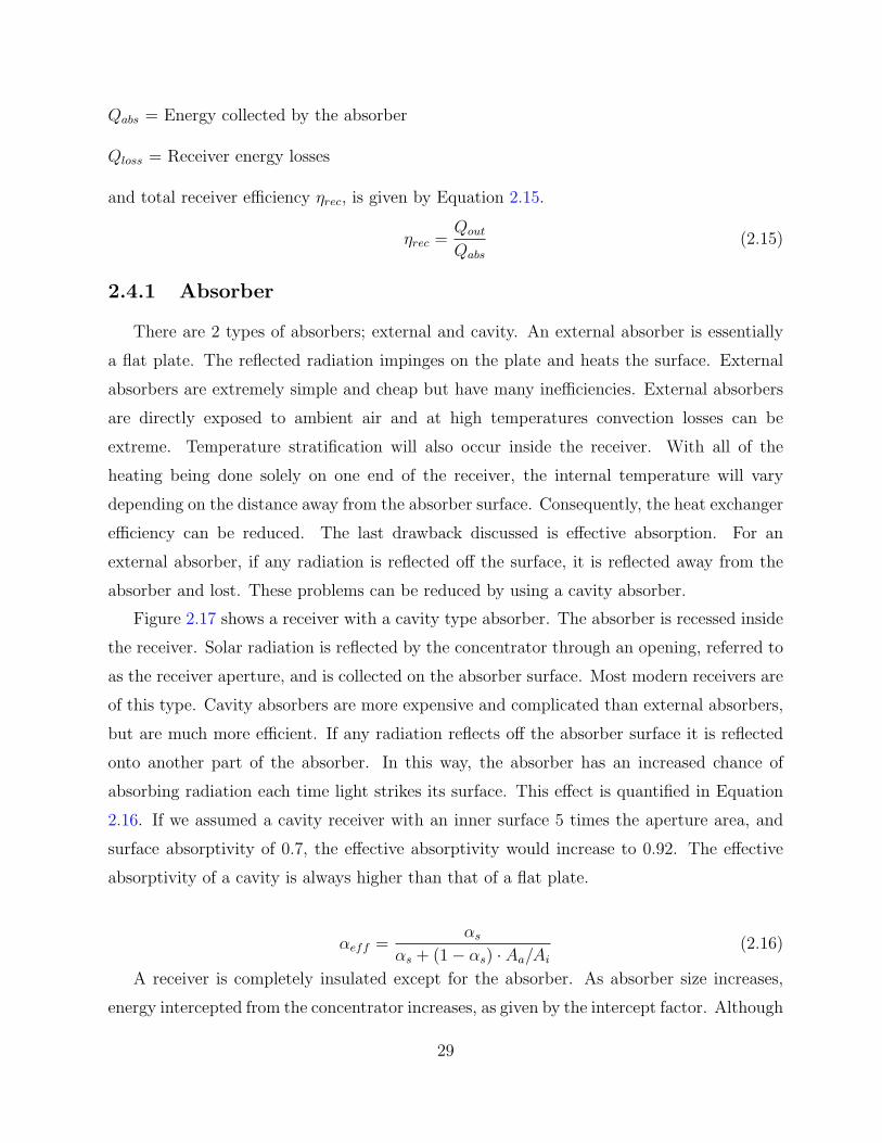
Figure 2.17 shows a receiver with a cavity type absorber. The absorber is recessed inside
the receiver. Solar radiation is reflected by the concentrator through an opening, referred to
as the receiver aperture, and is collected on the absorber surface. Most modern receivers are
of this type. Cavity absorbers are more expensive and complicated than external absorbers,
but are much more efficient. If any radiation reflects off the absorber surface it is reflected
onto another part of the absorber. In this way, the absorber has an increased chance of
absorbing radiation each time light strikes its surface. This effect is quantified in Equation
2.16. If we assumed a cavity receiver with an inner surface 5 times the aperture area, and
surface absorptivity of 0.7, the effective absorptivity would increase to 0.92. The effective
absorptivity of a cavity is always higher than that of a flat plate.
αeff =αs
αs + (1− αs) · Aa/Ai(2.16)
A receiver is completely insulated except for the absorber. As absorber size increases,
energy intercepted from the concentrator increases, as given by the intercept factor. Although
29

Figure 2.17: Cavity Receiver [8]
as this happens, thermal losses to the environment also increase. To optimize absorber
size Equation 2.17 is used. In this equation absorbed radiation (Qin) is a function of the
characteristic absorber diameter “L” and the angular error of the concentrator “Γ”. Energy
losses (Qloss) are primarily a function of absorber diameter for an ideal cavity.
Qopt = Qin(L,Γ)−Qloss(L) (2.17)
2.4.2 Heat Storage
Many applications for working fluids require a steady thermal output. Heat may be
stored in the receiver to act as a damper for heat transfer. When momentary cloud cover
blocks energy input to the system the working fluid can obtain energy from the stored heat.
If a receiver is producing steam to run a turbine and the thermal input decreased, the turbine
blades could be damaged if liquid water is injected. A system equipped with heat storage
could generate the steam after decreased solar input, decreasing the risk of outputting liquid
water.
Energy can be stored in any material by increasing its temperature. The amount of
energy stored is proportional to the mass, heat capacity and temperature increase. The
storage capacity of a mass can be made more efficient if it undergoes a phase change. This
30
effect increases thermal storage without increasing receiver temperature. The total energy
stored in a material that undergoes a phase change is given in Equation 2.18.
Qs = m[Csolid(T∗ − T1) + λ+ Cliquid(T2 − T ∗)] (2.18)
where:
Qs = Energy storage
m= Mass of material
Csolid= Heat capacity of solid phase
Cliquid= Heat capacity of liquid phase
T1= Initial material temperature
T ∗= Phase change temperature
T2=Final material temperature
2.4.3 Heat Transfer
Most heat transfer in a concentrating collector system occurs at the receiver. Energy
from insolation is reflected onto the absorber and leaves the system via the working fluid and
thermal losses. Heat is lost through all three modes of heat transfer; radiation, conduction
and convection. The thermal efficiency of a concentrator system (ηtherm) is given by Equation
2.19.
ηtherm = Qout/Qin = 1− QL
Qin
(2.19)
in this equation:
Qin = Adish · I
QL = Qrad +Qconv +Qcond
and:
Qin = Energy incident on dish
I= Direct normal insolation
Qout = Energy absorbed by working fluid
31

Figure 2.18: Radiant Flux of a Blackbody [2]
2.4.4 Radiation
All bodies emit radiation. The amount of energy a body emits depends upon the surface
temperature and emissivity, ε. Emissivity is a material property that describes the rate of
emission for a surface relative to a blackbody. A blackbody is a material that emits energy
at a rate prescribed by Planck’s law of blackbody radiation, as shown in Figure 2.18.
Equation 2.20 gives the net energy loss due to radiation for a cavity receiver[7]. Inside a
cavity some radiation will reflect back to the cavity walls. To account for this effect, a term
called effective emissivity (εeff ) is used. Equation 2.21 gives effective emissivity for a cavity
receiver [7].
Qrad = εeff · σ · Aa · (T 4s − T 4
∞) (2.20)
εeff =εcav
εcav + (1− εcav) · (Aa/Acav)(2.21)
In this equation:
εeff = Effective emissivity of cavity
εcav = Emissivity of cavity surface
σ = Stefan-Boltzmann constant
32
Aa = Surface area of aperture
Acav = Surface area inside cavity
Ts = Surface temperature of receiver
T∞ = Temperature of surroundings
2.4.5 Convection
Convection transfers energy from the absorber surface directly to the air in contact with
it. When the air is stationary it is referred to as natural convection and when it is in
motion it is referred to as forced convection. Equation 2.22 gives the heat loss due to natural
convection for a cavity [20].
Qcond = h · Acav · (Ts − Tamb) (2.22)
h =Nuf · kamb
L(2.23)
Nu = 0.088 ·Gr13 · (Ts/Tamb).18 · cos θ2.47 · (L/Dcav)
s (2.24)
in this equation:
s = 1.12− 0.98 · (L/Dcav)
Gr =g · β · (Ts − Tf ) · L3
υ2
and:
h = Average heat transfer coefficient
Acav = Cavity area
Ts = Temperature of receiver surface
Tamb= Ambient fluid temperature
Tf= Average fluid temperature
Nu= Nusselt number
Gr= Grashoff number
kf= Thermal conductivity of ambient fluid
L= Characteristic length of aperture opening (diameter)
Dcav= Diameter of cavity
33

υ = Kinematic viscosity
θ = Angle receiver makes with zenith (at θ = 0◦ the receiver is horizontal)
g= Gravity
β= Volumetric thermal expansion coefficient
At a tilt angle of θ = 90◦ (vertical), the air inside a cavity becomes trapped. The hot,
buoyant air inside the cavity cannot escape and convection losses are nearly eliminated. As
the tilt angle decreases (θ < 90◦) a dramatic increase in heat loss occurs as the lighter air
begins escaping from the cavity. In this case buoyancy works to aid in heat loss.
To reduce convective losses a translucent cover can be placed over the aperture. A cover
allows the insolation to transmit through the material while trapping gas inside. Convection
would still occur at the surface of the cover, but it would be reduced due to the reduction in
exposed surface area. Convective loss can be calculated in this case by modeling the cover as
an inclined flat plate. Using equation 2.25 gives the Nusselt number for an inclined flat plate,
which can be used with equation 2.22 to calculate convective losses. Figure 2.19 compares
the energy loss for an open and covered cavity. This example assumes an aperture diameter
of 30 cm, and cavity area ratio of 5.
Nu = 0.56(Gr · Pr · cos θ)14 (2.25)
where:
θ < 88◦; 105 < Gr · Pr · cos θ < 1011
All properties are evaluated at a reference temperature Te, except for β which is evaluated
at Tβ:
Te = Tw − 0.25(Ts − T∞)
Tβ = T∞ + 0.50(Ts − T∞)
2.5 Steam Boiler Design
A boiler is a closed vessel where water or another working fluid is heated. Most
conventional boilers burn some fuel and pass the superheated exhaust gases into a boiler
to boil a working fluid. Designs of boilers are classified by their heat transfer process.
34

Figure 2.19: Convection Loss vs. Tilt Angle for Open and Covered Cavities
Fire tube boilers look similar to conventional hot water heaters. Water is kept in a sealed
container with empty space above it to hold the steam. Hot exhaust gases are passed through
tubes inside the container, heating the water on the outside surface of the tubes. This causes
water to boil and steam to accumulate at the top of the vessel.
Water tube boilers have exactly the opposite design. Hot exhaust gases are sent into an
open vessel and the water is passed through tubes in the vessel. Water is heated on the
inside surface of the tubes, where it is converted to steam. This water/steam mixture then
flows together through the tubes. A conventional design of a water tube boiler can be seen
in Figure 2.20. The major parts of the water tube boiler are: the steam drum, mud drum,
downcomer tube and riser tube. Water flowing through the risers is heated by the flue gases.
Hot water and vapor rises into the steam drum where they are separated. The steam exits
the top of the drum and the liquid water falls due to buoyancy down the downcomer tube.
Incoming feedwater can be pumped into the steam drum or mud drum.
35

Figure 2.20: Water Tube Boiler [11]
2.5.1 Boiling
Phase change of a working fluid only occurs at a contact interface. Boiling can occur at
the solid-liquid contact, as in water in a hot pan, as well as a liquid-vapor interface. For
example, if hot gas was passed over a pool of water, boiling would occur at the surface of the
water. We will only be concerned about the first case for this application. At the solid-liquid
interface two types of boiling have been identified: nucleate and film. Nucleate boiling refers
to the formation and release of steam bubbles on the solid surface with liquid water still
wetting the contact surface. Film boiling occurs when the water flow rate in the tube in
contact with the wall is not high enough to remove steam bubbles being produced. Steam
accumulates until the tube wall is covered with a continuous film of vapor [21]. This film acts
as an insulator separating the heating surface from the working fluid. Beyond this point,
increasing the temperature of the tube surface results in a net decrease in heat transfer.
This point is marked B in Figure 2.21. This figure shows the boiling curve for heat transfer
coefficient (h) and net heat transfer (q). It can be seen that the heat transfer coefficient
decreases after point B′. This drop precedes the reduction in net heat transfer because the
film layer is still very thin. As the film layer increases, the effect on net heat transfer is
observed. An important aspect of boiler design is making sure that enough fluid is flowing
through the boiler tubes to prevent film boiling.
A well designed boiler has a steady stream of water flowing up the riser tubes constantly
36

Figure 2.21: Typical Boiling Curve [10]
feeding the steam drum. There are two ways flow can occur inside the boiler: forced and
natural circulation. Forced circulation employs pumps inside the boiler to force flow in the
desired direction. Natural circulation, which is commonly used in industrial boilers, utilizes
the natural density difference of the cold water in the downcomers and the less dense hot
water vapor mixture in the risers. The pressure difference in the two sections creates the
force needed to keep flow moving through the system.
Steam separation is also an important aspect to designing a steam drum. If the steam
does not separate from the water the steam outlet tube will contain unwanted liquid that
can damage turbine blades or adversely affect other applications that require pure steam.
An open boiler has an unobstructed interface between the liquid water and steam. If the
steam velocity leaving the water’s surface is low (less than .9 m/sec) the steam bubbles will
separate from the liquid droplets [9]. If the rate is too high, water droplets will be carried
into the steam outlet line. For a unit with a higher velocity of steam production, gravity
alone is not enough to separate the steam from the liquid. In this case steam separators
must be utilized to facilitate gravitational separation. Simple types of steam separators form
a barrier between the steam escaping the liquid and the exit tube. This forces the steam to
take a longer path giving more time for gravity to separate the steam from any liquid that
37

has been carried with the steam.
38
CHAPTER 3
EXPERIMENTAL SETUP
A 14 m2 parabolic dish solar concentrator was fabricated and tested at the SESEC
facilities at Florida State University. The concentrator is referred to as Solar 2 and it
consists of a new concentrator and receiver assembly. The original steel frame and tracking
system were kept from the first concentrator built at SESEC, Solar 1. This chapter includes
details on design and fabrication for the concentrator system.
3.1 Parabolic Dish
The parabolic dish was constructed out of fiberglass, which was chosen because of its
ability to form to any mold. The entire concentrator system was limited in size by the
parabolic dish. The largest mold that was practical to make in house was limited to a 1.2
m (4 ft) x 2.4 m (8 ft) plywood sheet. It was important to fabricate the system by hand
to ensure cost efficiency and simplicity of manufacturing and assembly. To maximize the
concentrator size, small sections were made and fitted together to form a continuous dish.
The dish was comprised of eleven identical pieces and each piece was a 32 degree wedge of
the full dish. This left 8 degrees open for the receiver arm, which will be discussed below.
The effective radius at the outer rim of the dish was 2.13 m and the greatest width of each
section was 1.1 m. Each section was handmade at SESEC using vacuum molding techniques.
To create the mold that mimicked the parabolic shape, a plug was first needed. A plug is
a piece that replicates the outer contour of the final product. The plug consisted of 0.16 cm
thick plywood sheet pressed onto verticle plywood ribs. The ribs were shaped to the profile
of the dish given in Equation 3.1.
y =1
8.53m× x2 (3.1)
39
Figure 3.1: Bare Concentrator Wedge
A thin plywood sheet was placed onto the ribs, taking the exact shape of the panels desired.
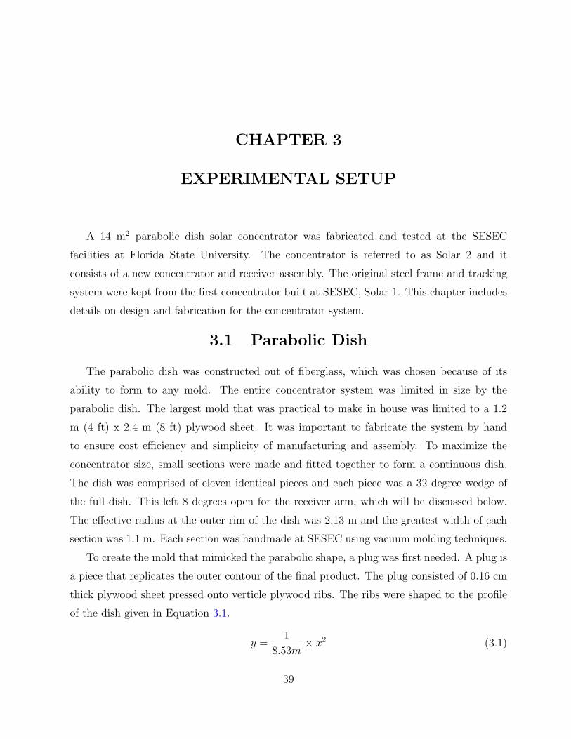
A plywood box framed the plug, sealing it tight. This held the liquid plaster that was poured
into the cavity. The plaster took the negative shape of the plug and created a mold.
To construct the fiberglass concentrator sections, a foam sheet was laid between sheets
of fiberglass cloth. The foam core strengthens the panels without greatly increasing weight
because the foam does not absorb any of the hardening resin. The fiberglass and foam were
then laid on the mold, taking the panels final shape. A plastic bag was wrapped around
both the fiberglass and mold and a vacuum was pulled on the bag. Suction from the bag
held the fiberglass tightly to the contour of the mold. Resin was then drawn into the bag,
soaking into the sheets of fiberglass. The result after hardening was a strong, lightweight and
durable panel. Each of the eleven sections weighed approximately 17 lbs. Figure 3.1 shows
a completed wedge after it had been sanded. All of the wedge pieces were bolted together,
then bolted to the steel frame discussed below.
A focal length of 2.1 m was chosen to give the dish a rim angle of 53◦. A greater
rim angle (shorter focal length) would decrease the acceptance angle of radiation into the
absorber cavity. A lesser rim angle (longer focal length) would increase strain on the receiver
arm and cause the optics to be more sensitive to error in the dish. The finished concentrator
is shown in Figure 3.2
40

Figure 3.2: Fully Assembled Concentrator
3.2 Reflective Surface
The reflective material used for this project is a silver polymer film produced by
ReflecTech. This film reflects 94% of the solar spectrum and lasts 10 years in an outdoor
environment. This particular material was chosen for its extremely high reflectivity and
flexibility of application. The film has an adhesive backing that can be applied easily to
any flat surface. One drawback of the product is that the film is very thin and extremely
susceptible to ‘print-through’. This occurs when the film contours to imperfections on the
applied surface and results in decreased optical clarity. This is a major problem when using
fiberglass as the concentrator structure. Fiberglass resin hardens to the cloth, leaving a
crisscross pattern of hardened fiberglass strands, which is a less than ideal surface for the
ReflecTech. Therefore, great care was given to surface preparation of the fiberglass. Initially,
all of the panels were covered and sanded with Bondo surface prep. This smoothed out
the print pattern of the fiberglass panels. However, the durability of the surface prep was
questioned during the painting process, and the panels were ultimately sanded down with
an industrial sander. A base paint was then sprayed directly to the sanded fiberglass. This
41

Figure 3.3: Mounting Frame
still left a small amount of ‘print-through’ on the reflective surface. The optical error due
to this effect is believed to be the same order of magnitude as the error in the curvature of
the dish surface. Because the print through error is random it did not greatly amplify the
surface error. This situation is acceptable given the advantages that the material brings. A
better surface preparation solution needs to be found if the curvature of the surface slope
was corrected.
3.3 Frame
The horizontal mount system has two axes of movement that independently track the
altitude and azimuth motion of the Sun. Figure 3.3 shows the mount system used for Solar
2. The azimuth pivot marked “D” follows the east-west movement of the sun throughout
the day. This pivot is made from 0.6 cm thick steel L-brackets that are 5.1 cm wide. The
azimuth pivot is controlled by a linear actuator which is mounted to the altitude pivot under
the point marked “C”. The altitude pivot follows the north-south movement of the Sun.
This pivot is made from 0.6 cm square tubing that is 10 cm wide, with 1.3 cm steel plates
extending up from the ends of the tubing.
The altitude pivot is mounted to the zenith pivot marked “B” in Fig 3.3. This pivot is
normally stationary and bolted tight. This section has the ability to rotate around the zenith
axis to align with celestial North. The zenith pivot is made from 0.6 cm steel plates and
42

Figure 3.4: Receiver Assembly and Connection Ring
welded to a sleeve cap which fits over a 12.7 cm nominal steel pipe. This steel pipe is bolted
by three 1.6 cm bolts to the 15.2 cm (6 in) XS nominal steel foundation pipe marked “A”.
The foundation pipe rises 1.2 m above a 10.2 cm deep concrete slab. It extends 4.3 m into
a 0.5 m diameter concrete backfilled hole. The foundation is designed to handle the forces
and moments of a 4.3 m diameter dish in winds up to 49 mps (110 mph). Full engineering
drawings for the foundation can be found in Appendix E.
Atop the mount system sits the connection ring. This 0.95 cm thick steel ring is 10.2
cm wide and 1.47 m in diameter. It is welded to the azimuth frame. Figure 3.4 shows the
connection ring, marked “F”. This ring has 0.95 cm slots machined out in which L-brackets
are bolted to. Twelve 0.95 cm L-brackets, 10.2 cm in length, bolt to the steel ring to the
flange of each panel.
The receiver is held in place by a single support arm. The arm is connected to a 7.6
cm square steel tube welded to the azimuth frame. This tubing is marked ”E” in Figure
3.4. Extending vertically at the end of this piece are two steel plates. Three 1.6 cm holes
are drilled through the plates. Between the plates, 7.6 cm aluminum tubing is inserted and
43
bolted in. Two of the bolts can be removed to allow the receiver arm to pivot around the
remaining bolt, lowering the receiver to ground level. This allows easy access for repairs and
changes to configuration during testing. The aluminum arm is marked ”G” in Figure 3.4. It
is made from two 7.6 cm pieces of aluminum square tubing. The vertical arm section is 1.92
m long and the angled section is 1.33 m long. An aluminum plate is welded at the end of
the arm. This plate has an array of bolt holes aligned vertically that allow the receiver to
be attached at differing heights. For different arrangements of aperture covers, the receiver
can be adjusted closer and further from the concentrator focal point.
3.4 Receiver
The receiver for this system acts as an absorber, boiler, and heat storage unit. A cavity
type absorber is used due to its high absorption efficiency and low heat loss. Surrounding
the absorber inside the receiver is 10 kg of sodium nitrate. This salt acts as a heat transfer
and storage media and 0.6 cm diameter copper tubing was coiled through it. The working
fluid is pumped through the tubing where heat is transfered to the fluid.
To find the optimum cavity size, heat losses and incident radiation must be estimated
based on aperture (cavity opening) diameter. Figure 3.5 shows the estimated energy absorp-
tion versus aperture diameter. Heat loss is dependent upon cavity geometry, orientation,
and surface emissivity. Calculations were made assuming negligible wind. In reality the
convective term will be greater, making the losses almost equal. The incident radiation was
estimated for a concentrator with an error 4 times that of the industrial standard. This
is one of the major drawbacks of a low budget. For perfect concentrator efficiency, the
incident radiation term in Figure 3.5 takes the shape of a step function, instantly reaching
maximum radiation of about 6150 W. The large slope in the curve shows the effect of
decreased efficiency. At the optimum diameter of 15 cm, only 80% of reflected radiation
passes through the aperture and the estimated Sun to absorbed energy efficiency is 42%.
The cavity depth was chosen such that 85% of reflected radiation strikes the cylindrical
cavity absorber wall, and 15% of radiation was absorbed by the top of the cavity. The
resulting cavity depth is 15 cm. For deeper cavities less radiation will strike the top of the
cavity, resulting in an uneven temperature distribution inside the cavity. For shorter cavities
the concentration ratio will be higher, increasing cavity temperature as well as thermal losses.
Figure 3.6 shows an exploded view of the receiver assembly.
44

Figure 3.5: Energy Absorption vs. Aperture Diameter
Figure 3.6: Exploded View of Receiver
45
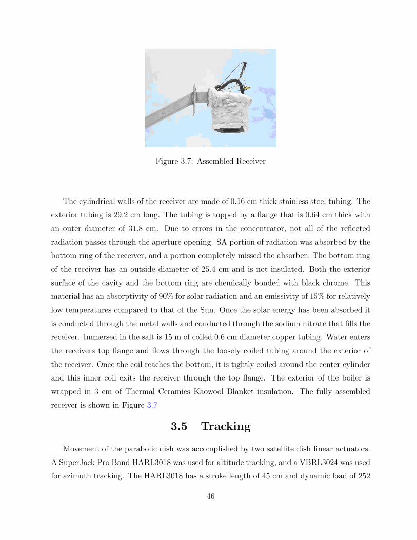
Figure 3.7: Assembled Receiver
The cylindrical walls of the receiver are made of 0.16 cm thick stainless steel tubing. The
exterior tubing is 29.2 cm long. The tubing is topped by a flange that is 0.64 cm thick with
an outer diameter of 31.8 cm. Due to errors in the concentrator, not all of the reflected
radiation passes through the aperture opening. SA portion of radiation was absorbed by the
bottom ring of the receiver, and a portion completely missed the absorber. The bottom ring
of the receiver has an outside diameter of 25.4 cm and is not insulated. Both the exterior
surface of the cavity and the bottom ring are chemically bonded with black chrome. This
material has an absorptivity of 90% for solar radiation and an emissivity of 15% for relatively
low temperatures compared to that of the Sun. Once the solar energy has been absorbed it
is conducted through the metal walls and conducted through the sodium nitrate that fills the
receiver. Immersed in the salt is 15 m of coiled 0.6 cm diameter copper tubing. Water enters
the receivers top flange and flows through the loosely coiled tubing around the exterior of
the receiver. Once the coil reaches the bottom, it is tightly coiled around the center cylinder
and this inner coil exits the receiver through the top flange. The exterior of the boiler is
wrapped in 3 cm of Thermal Ceramics Kaowool Blanket insulation. The fully assembled
receiver is shown in Figure 3.7
3.5 Tracking
Movement of the parabolic dish was accomplished by two satellite dish linear actuators.
A SuperJack Pro Band HARL3018 was used for altitude tracking, and a VBRL3024 was used
for azimuth tracking. The HARL3018 has a stroke length of 45 cm and dynamic load of 252
46

Figure 3.8: Assembled Linear Actuators
kg. The VBRL3024 has a stroke length of 61 cm and a dynamic load of 680 kg. A stronger
actuator was needed on the azimuth axis due to the extreme angles needed in tracking,
specifically when approaching horizontal. The large moment caused by the receiver at these
angles requires an extremely powerful actuator. Power for the actuators was provided by
the local electrical grid. However, this system can be powered remotely by a small PV panel
and two 24V batteries, as was done on Solar 1. Figure 3.8 shows the assembled actuators.
The tracking system was controlled by a dual axis tracking sensor shown in Figure 3.9.
The LED3X sensor was built by Red Rock Energy. It has four LEDs attached to a circuit
board. The relative intensity of radiation for each LED is measured and when there is a
disparity between two LEDs the circuit allows movement of the actuators to re-align the
system.
3.6 Data Acquisition and Instrumentation
System testing consisted of running water through the heated boiler. The temperature
rise and mass flow rate of the water was measured to calculate thermal power output. Three
thermocouples were used for data acquisition. The thermocouples were placed at the water
inlet, inside the thermal bath, and at the exit of the receiver. A schematic of the receiver
47

Figure 3.9: Dual Axis Tracking Sensor
during testing is shown in Figure 3.10. The thermocouples used were Omega K-type (CASS-
18U-6-NHX) and were connected to data acquisition hardware using K-type thermocouple
wires. A National Instruments Signal Conditioning Board (SCB-68) routed the signal to a
National Instruments data acquisition card, model DAQCard -6024e. The card had a 12 bit
resolution with sampling rate of 1 kS/s. The FSO during testing was 10 V. The DAQ card
had a corresponding absolute accuracy during testing of 2.44 mV.
Both the water and pumping power for testing was provided from the local water tap.
The average pressure at water inlet was 60 psi, and the flow rate was controlled and measured
using a ball float flow meter with control valve. The valve had a flow range of 2-25 GPH
with an accuracy of ±4%. Measurements were taken by hand and logged into the LabVIEW
software.
A pyrheliometer was used to measure direct normal insolation during testing. The
instrument used was an Eppley Model NIP. This pyrheliometer was mounted on a power-
driven equatorial mount for continuous readings. The unit has a sensitivity of approximately
8 µV/Wm−2, and holds linearity of ±0.5% from 0 to 1400 Wm−2. The unit can be seen in
Figure 3.11.
48

Figure 3.10: Schematic of Test Setup
Figure 3.11: Eppley Nominal Incidence Pyrheliometer
49

CHAPTER 4
RESULTS AND DISCUSSION
This chapter contains results and analysis for testing performed at SESEC facilities in
the Spring of 2009. Tests were performed to determine the thermal conversion efficiency
of the concentrator system. Water was pumped through the central receiver where it was
heated and the flow rate and temperature rise of the water were recorded to determine the
collected energy. To calculate solar energy input, a pyrheliometer was used to measure direct
beam insolation. With this information the thermal collection efficiency for the system was
found. The system was characterized by estimating thermal losses for each sub-component.
The chapter concludes with an economic analysis.
4.1 Thermal Efficiency Results
4.1.1 Steady State Thermal Testing
Tests were performed to determine total thermal conversion efficiency. In these tests,
water inlet water at 20 ◦C was heated by the receiver to temperatures under 100 ◦C. By not
flashing the working fluid, a steady inlet flow was achieved that allowed accurate collected
energy measurements. Results from steady state thermal conversion tests are shown in
Figures 4.1 through 4.3. The figures show outlet water temperature, salt bath temperature
and insolation during each test. The average conversion efficiency at a cavity angle of 53
degrees was 39%.
4.1.2 Superheated Steam Production
A series of tests were conducted to produce superheated steam. In these tests the receiver
was heated without water flowing through it, until it reached a temperature of 400 ◦C. Water
50

Figure 4.1: Testing Performed Feb 23, 2009
Figure 4.2: Testing Performed March 02, 2009
51
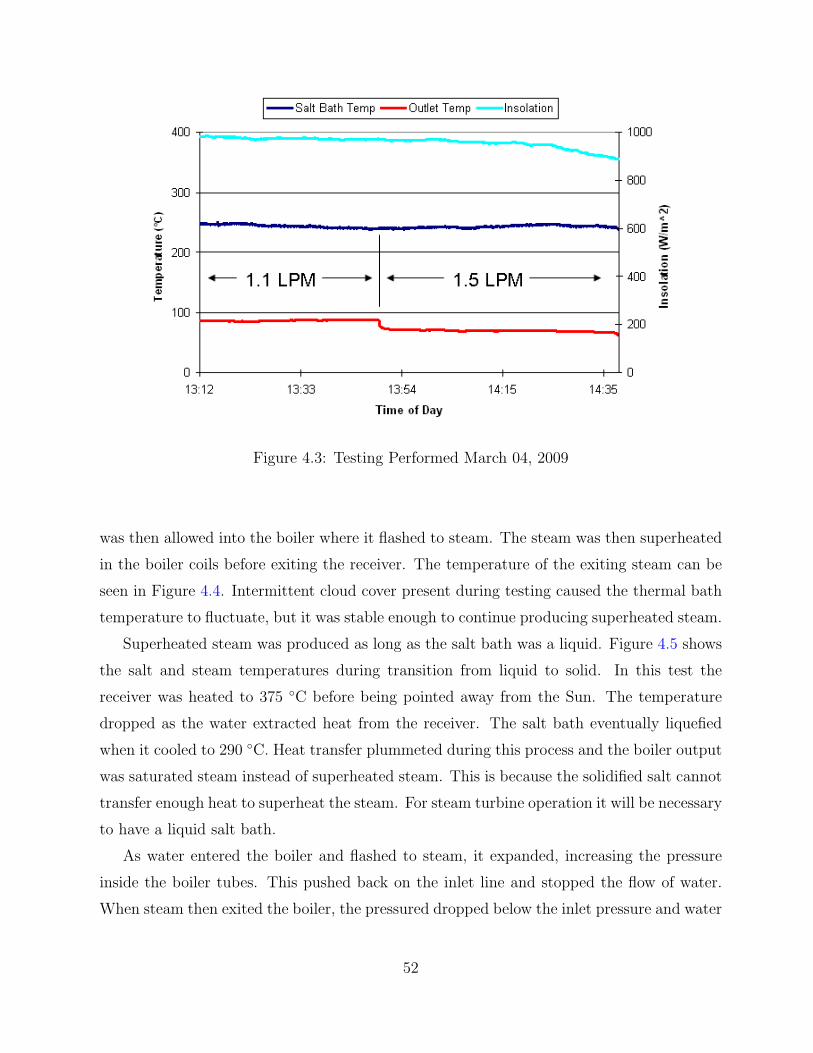
Figure 4.3: Testing Performed March 04, 2009
was then allowed into the boiler where it flashed to steam. The steam was then superheated
in the boiler coils before exiting the receiver. The temperature of the exiting steam can be
seen in Figure 4.4. Intermittent cloud cover present during testing caused the thermal bath
temperature to fluctuate, but it was stable enough to continue producing superheated steam.
Superheated steam was produced as long as the salt bath was a liquid. Figure 4.5 shows
the salt and steam temperatures during transition from liquid to solid. In this test the
receiver was heated to 375 ◦C before being pointed away from the Sun. The temperature
dropped as the water extracted heat from the receiver. The salt bath eventually liquefied
when it cooled to 290 ◦C. Heat transfer plummeted during this process and the boiler output
was saturated steam instead of superheated steam. This is because the solidified salt cannot
transfer enough heat to superheat the steam. For steam turbine operation it will be necessary
to have a liquid salt bath.
As water entered the boiler and flashed to steam, it expanded, increasing the pressure
inside the boiler tubes. This pushed back on the inlet line and stopped the flow of water.
When steam then exited the boiler, the pressured dropped below the inlet pressure and water
52

Figure 4.4: Superheated Steam Production March 09, 2009
then flowed back into the boiler. This resulted in an oscillating flow rate. The manual flow
meter used was incapable of measuring unsteady flow of this type and as result no flow rate
data is presented here. An automated data logging flow meter that can handle fluctuating
flow rates must be used to get an accurate reading. This will be required to discover the
conversion efficiency of the system while producing superheated steam.
4.1.3 Thermal Storage
Thermal storage in the receiver is intended to dampen the effects of changing insolation.
The objective is to keep the output temperature relatively steady during intermittent cloud
cover, as was demonstrated with the production of superheated steam as shown in Figure
4.4. The output temperature dropped only 54 ◦C when the Sun was blocked by clouds
for nearly 15 minutes from 13:34 to 13:50. The length of time the receiver stays heated
will depend on the duration of the blocked sunlight and the amount of energy removed by
the working fluid. The output steam remained superheated for the duration of the cloud
cover. If the output steam had been connected to a turbine, the thermal storage would have
53

Figure 4.5: Testing Performed March 02, 2009Display of Salt Bath Phase Change
ensured continuous operation. A similar effect is seen in Figure 4.6, which shows testing
with intermittent cloud cover when the salt bath was a solid. The temperature drop was
slower than in the superheated case due to the lower water flow rate.
Heat is also stored in the phase change of the bath salt. When the boiler reaches the
phase change temperature of the salt, the bath temperature is momentarily constant. This
increases the time that the boiler can produce superheated steam when cooling down. Figure
4.5 shows the output and salt bath temperature during phase change. It can be seen that
the amount of heat released during phase change is small. This is due to the fact that most
of the thermal mass in the receiver is in the stainless steel, while the salt holds only a small
fraction of the heat in the receiver. This has unintended consequences during warm up and
cool down and is discussed below.
A clear example that the salt bath holds only a portion of the thermal mass is shown in
Figure 4.7. In this figure two different salt bath heating rates can be seen; A and B. Rate A
corresponds to heating of the entire receiver, salt and steel, which occurs at 65 ◦C/hr. Rate
B corresponds to when the heat has been drawn from the salt bath by the working fluid, but
54

Figure 4.6: Testing Performed Sept 04, 2008 0.7 LPM
the steel is still hot. In this case the salt heats up at 410 ◦C/hr, over 6 times that of rate A.
This shows that when the salt bath and steel housing are at the same temperature, most of
the heat goes to heating the steel. This is detrimental because the steel does not give up its
heat quickly to the working fluid and therefore, it is wasted energy.
4.1.4 Warm-up and Cooling-down
The large thermal mass of the receiver generally hurts performance. The worst effect on
the system can be seen during warm-up of the receiver. Figure 4.8 shows the initial warm up
temperature profile. The heating rate for the salt bath was 65 ◦C/hr, which was the same
as rate ‘A’ marked in Figure 4.7. For steady state testing the salt bath reached equilibrium
at 250 ◦C. It took 3.8 hours for the receiver to heat up to equilibrium temperature when
water was flowing through the receiver from start-up. The quickest way to heat the receiver
was to do so without water flowing through it. After the receiver had reached 250 ◦C, it was
removed from the focal point and water was allowed to pass through it. Initially the water
flashed to steam and the flow rate was reduced considerably. After waiting for the salt bath
55

Figure 4.7: Testing Performed February 24, 2009 1.0 LPM
to cool so that no steam exited the receiver, it was again placed in the focal point where the
salt was heated at rate B until it reached equilibrium. This complicated warm-up procedure
could have been avoided if less steel was used in the construction of the receiver.
4.1.5 Tracking Error
The tracking sensor used for testing was not always accurate. The LED tracker was
mounted to the receiver arm. During testing the large amounts of torque placed on the arm
by the receiver caused the arm to bend. In particular, when the azimuth angle was greater
than 45◦ the receiver arm bending caused the tracker mounted to it to err. Figure 4.9 shows
the tracking error during late hours. The oscillating receiver temperatures are seen with
relation to the steady insolation. The tracking system has a difficult time correcting for
changes in both altitude and azimuth angle.
Tracking error also occurs with intermittent cloud cover. The tracking mechanism was
designed to point at the brightest spot in the sky. When clouds cover the Sun, thinner
parts of the cloud shine the brightest. The tracking system then points to this spot. After
the cloud has passed, the system is not aimed at the Sun and must correct itself. This
56

Figure 4.8: Testing Performed Feb 22, 2009 1.5 LPM
Figure 4.9: Testing Performed Feb 19, 2009 1.3 LPM
57
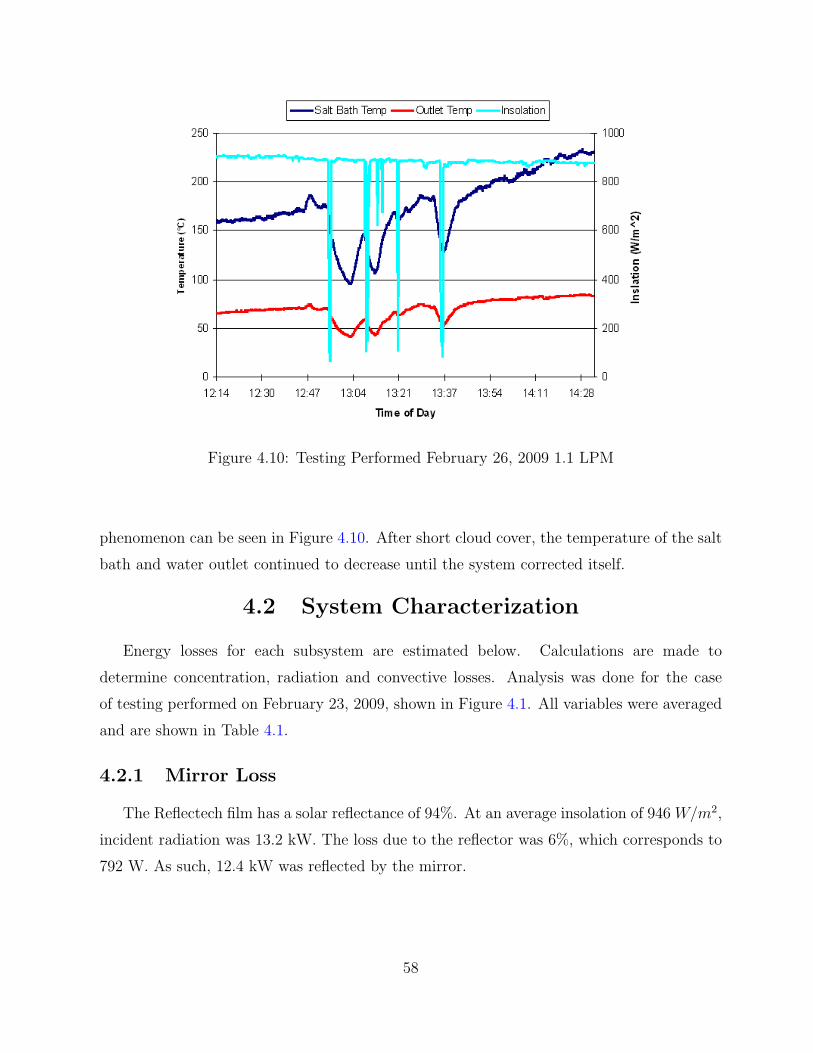
Figure 4.10: Testing Performed February 26, 2009 1.1 LPM
phenomenon can be seen in Figure 4.10. After short cloud cover, the temperature of the salt
bath and water outlet continued to decrease until the system corrected itself.
4.2 System Characterization
Energy losses for each subsystem are estimated below. Calculations are made to
determine concentration, radiation and convective losses. Analysis was done for the case
of testing performed on February 23, 2009, shown in Figure 4.1. All variables were averaged
and are shown in Table 4.1.
4.2.1 Mirror Loss
The Reflectech film has a solar reflectance of 94%. At an average insolation of 946 W/m2,
incident radiation was 13.2 kW. The loss due to the reflector was 6%, which corresponds to
792 W. As such, 12.4 kW was reflected by the mirror.
58

Table 4.1: Average Values for Testing Performed Feb 23, 2009
Cavity Angle (deg) 53Concentrator Area m2 13.98Absorber Surface Temp (◦C) 800Ambient Temp (◦C) 20Water Flow Rate (LPM) 1.5Inlet Temp (◦C) 19.5Outlet Temp (◦C) 69.2Salt Bath Temp (◦C) 243Insolation (W/m2) 946Qin (kW) 13.2Qout (kW) 5.2Thermal Efficiency (%) 39
4.2.2 Concentrator Geometry Loss
Angular error was estimated for the fiberglass dish to determine the intercept factor. The
error was estimated to the nearest integer multiple of the industrial standard error, which is
6.7 mrad. A series of boards with a center hole cut out were constructed. The center hole
was cut with the diameter equal to the 99% cutoff diameter for a particular standard error.
For the case of 5 standard errors (5*6.7 mrad angular error) the 99% cutoff diameter for a
concentrator with a focal length of 2.13 meters is 38.5 cm. This means 99% of the reflected
light should shine inside this circle. The fiberglass concentrator built corresponded closest
to an angular error 6 times the industrial standard. The concentrator angular error was 40.2
+/- 6.7 mrad. The intercept factor for this error is plotted in Figure 4.11 with respect to
aperture diameters. It can be seen that 60%, or 7.44 kW, of the radiation strikes inside the
cavity aperture and 25%, or 3.1 kW, of radiation strikes the absorber plate. The remaining
15% of reflected radiation was lost completely, which amounted to 1.86 kW.
4.2.3 Absorption Loss
When impinging radiation reflects off the absorber it is considered an absorption loss. The
absorptivity coefficient of the cavity and plate surface was 90%. As such, 10%, or 310 W, of
59

Figure 4.11: Intercept Factor for Solar 2
radiation that hit the absorber plate was lost. The cavity surface had the same absorptivity
as the plate, but it recaptured some of the reflected radiation. When light was reflected off
the surface it hit another surface, giving it a much higher chance of being absorbed. The
effective absorptivity of the cavity was 98.7%. Only 164 W was lost by reflection out of the
cavity. The total absorption losses were calculated to be 474 W.
4.2.4 Radiation Loss
Radiation losses were estimated for the cavity and plate absorber separately. Equation
2.20 gives energy lost due to radiation. For a cavity, the radiated energy is calculated using
the effective emissivity given in Equation 2.21. The emissivity of the black chrome coating
on the absorber surface is 0.15. For the absorber plate, the amount of radiated energy at
800◦C is 0.6 kW. The cavity helped to reduce radiation losses by recapturing radiated energy.
Even though the cavity surface area is nearly 4 times that of the absorber plate, the losses
were only slightly higher at 0.85 kW. The total loss from the absorber due to radiation was
calculated at 1.5 kW.
60

4.2.5 Convection Loss
Natural convection was the largest contributor to heat loss. At a cavity angle of 53◦
buoyancy forces kept air continuously moving over the absorber, taking great amounts of
heat. Using Equation 2.22 energy loss due to natural convection from a cavity can be found.
The convective heat loss from the cavity was calculated at 1.3 kW. The absorber plate was
modeled as an inclined flat plate. Equation 2.24 gives the average Nusselt number that must
be used with Equation 2.22 to find convection from an inclined plate. Natural convection
from the absorber plate was calculated at 1.1 kW. The total heat loss due to convection was
2.4 kW.
4.2.6 Remaining Thermal Loss
A simple First Law energy balance reveals that an additional 1.1 kW are lost. This is
due to a combination of many small losses. The largest being reflector wear, conduction and
imperfect insulation. The mirrored surface had a maximum reflective efficiency of 94%. In
reality the efficiency of the mirrored surface on Solar 2 was not this high. Dust and dirt
were blown onto the reflector and blocked sunlight. Discolorations formed on sections of the
mirror after water pooled on them for months. If the wear was enough to reduce reflectivity
to 90%, an additional 528 W were lost.
Conduction occurred at the joining of the receiver and the connection arm. This was
reduced as much as possible by placing insulation between the plates that are bolted together.
The insulation will conduct a small amount, but the stainless steel bolts that directly connect
the receiver to the arm are good conductors of heat.
The final major contributor is the insulation surrounding the receiver. The insulation
was not one continuous piece covering the receiver. Hot air could work its way out of the
insulation carrying heat with it. The insulation itself heated a small amount and convected
heat to the ambient air.
4.2.7 Reducing Losses
Figure 4.12 shows a breakdown of the relative losses for Solar 2. Convection, radiation and
concentrator geometry error make up 71% of all of the losses. Each of these three systems
is primarily dependent upon the angular error of the concentrator, which determines the
61
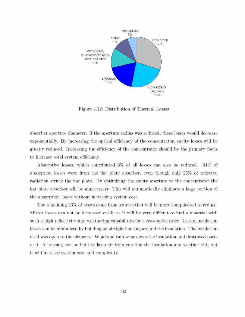
Figure 4.12: Distribution of Thermal Losses
absorber aperture diameter. If the aperture radius was reduced, these losses would decrease
exponentially. By increasing the optical efficiency of the concentrator, cavity losses will be
greatly reduced. Increasing the efficiency of the concentrator should be the primary focus
to increase total system efficiency.
Absorptive losses, which contributed 6% of all losses can also be reduced. 64% of
absorption losses were from the flat plate absorber, even though only 25% of reflected
radiation struck the flat plate. By optimizing the cavity aperture to the concentrator the
flat plate absorber will be unnecessary. This will automatically eliminate a large portion of
the absorption losses without increasing system cost.
The remaining 23% of losses came from sources that will be more complicated to reduce.
Mirror losses can not be decreased easily as it will be very difficult to find a material with
such a high reflectivity and weathering capabilities for a reasonable price. Lastly, insulation
losses can be minimized by building an airtight housing around the insulation. The insulation
used was open to the elements. Wind and rain wear down the insulation and destroyed parts
of it. A housing can be built to keep air from entering the insulation and weather out, but
it will increase system cost and complexity.
62
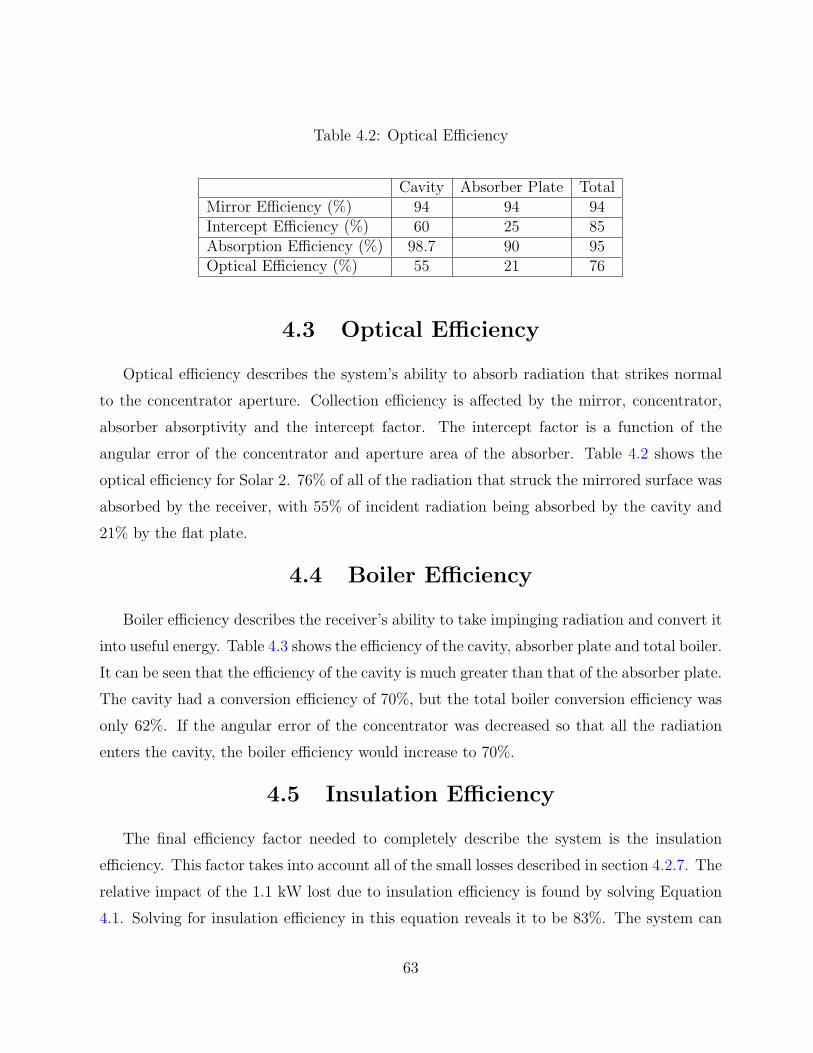
Table 4.2: Optical Efficiency
Cavity Absorber Plate TotalMirror Efficiency (%) 94 94 94Intercept Efficiency (%) 60 25 85Absorption Efficiency (%) 98.7 90 95Optical Efficiency (%) 55 21 76
4.3 Optical Efficiency
Optical efficiency describes the system’s ability to absorb radiation that strikes normal
to the concentrator aperture. Collection efficiency is affected by the mirror, concentrator,
absorber absorptivity and the intercept factor. The intercept factor is a function of the
angular error of the concentrator and aperture area of the absorber. Table 4.2 shows the
optical efficiency for Solar 2. 76% of all of the radiation that struck the mirrored surface was
absorbed by the receiver, with 55% of incident radiation being absorbed by the cavity and
21% by the flat plate.
4.4 Boiler Efficiency
Boiler efficiency describes the receiver’s ability to take impinging radiation and convert it
into useful energy. Table 4.3 shows the efficiency of the cavity, absorber plate and total boiler.
It can be seen that the efficiency of the cavity is much greater than that of the absorber plate.
The cavity had a conversion efficiency of 70%, but the total boiler conversion efficiency was
only 62%. If the angular error of the concentrator was decreased so that all the radiation
enters the cavity, the boiler efficiency would increase to 70%.
4.5 Insulation Efficiency
The final efficiency factor needed to completely describe the system is the insulation
efficiency. This factor takes into account all of the small losses described in section 4.2.7. The
relative impact of the 1.1 kW lost due to insulation efficiency is found by solving Equation
4.1. Solving for insulation efficiency in this equation reveals it to be 83%. The system can
63
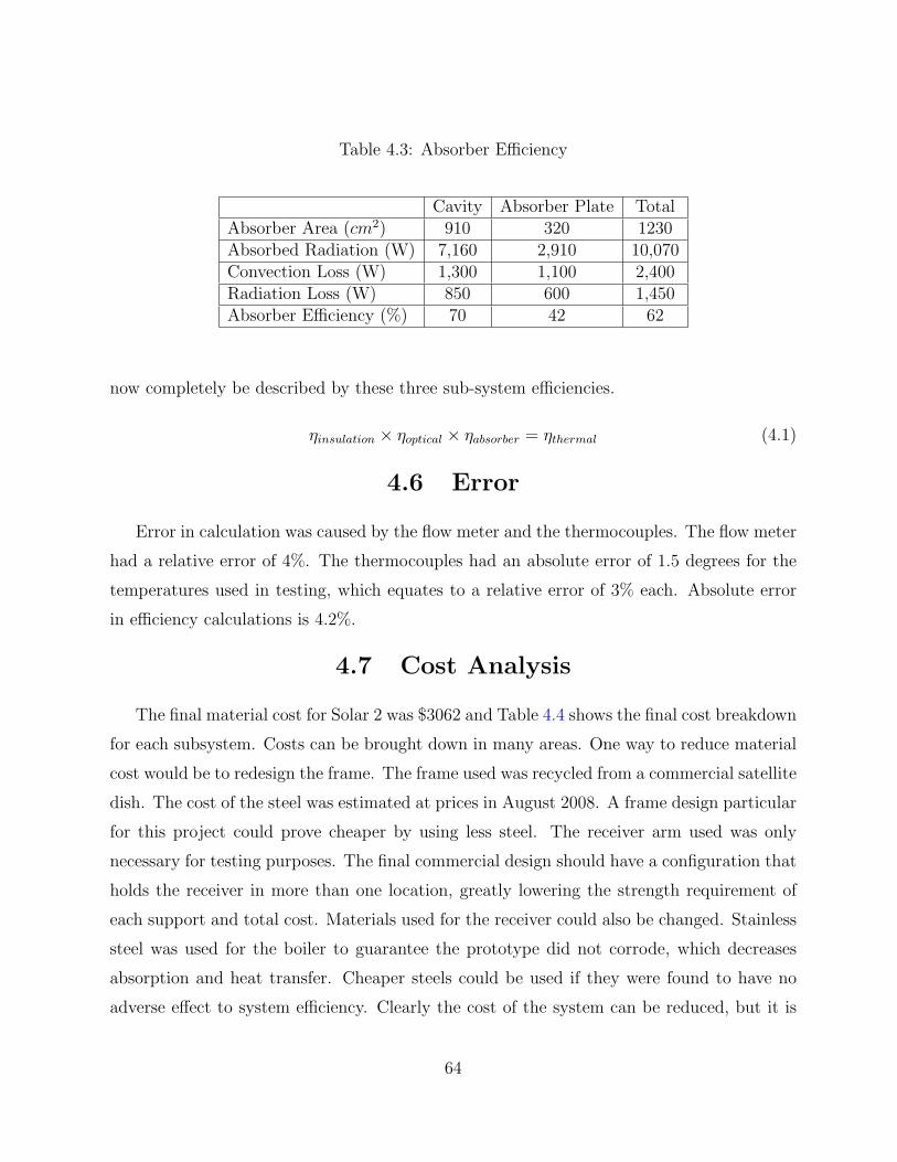
Table 4.3: Absorber Efficiency
Cavity Absorber Plate TotalAbsorber Area (cm2) 910 320 1230Absorbed Radiation (W) 7,160 2,910 10,070Convection Loss (W) 1,300 1,100 2,400Radiation Loss (W) 850 600 1,450Absorber Efficiency (%) 70 42 62
now completely be described by these three sub-system efficiencies.
ηinsulation × ηoptical × ηabsorber = ηthermal (4.1)
4.6 Error
Error in calculation was caused by the flow meter and the thermocouples. The flow meter
had a relative error of 4%. The thermocouples had an absolute error of 1.5 degrees for the
temperatures used in testing, which equates to a relative error of 3% each. Absolute error
in efficiency calculations is 4.2%.
4.7 Cost Analysis
The final material cost for Solar 2 was $3062 and Table 4.4 shows the final cost breakdown
for each subsystem. Costs can be brought down in many areas. One way to reduce material
cost would be to redesign the frame. The frame used was recycled from a commercial satellite
dish. The cost of the steel was estimated at prices in August 2008. A frame design particular
for this project could prove cheaper by using less steel. The receiver arm used was only
necessary for testing purposes. The final commercial design should have a configuration that
holds the receiver in more than one location, greatly lowering the strength requirement of
each support and total cost. Materials used for the receiver could also be changed. Stainless
steel was used for the boiler to guarantee the prototype did not corrode, which decreases
absorption and heat transfer. Cheaper steels could be used if they were found to have no
adverse effect to system efficiency. Clearly the cost of the system can be reduced, but it is
64

unsure whether it will be possible to reduce the system cost to the original goal of $1000.
The dramatic rise in the cost of materials, even in the period of fabricating this system, will
make it difficult to reach this goal.
65

Table 4.4: Material Costs
Frame and Foundation CostBase Tubing 6” SCH 80 Steel Tubing 17’ 350.00Concrete 1 sq yd bulk 100.00Connection Tubing 5” SCH 840 Steel Tubing 28’ 44.11Base Top .5” Steel Plate 6” x 4.5’ 84.62Altitude Axis 1/2” x 4” Steel Plate 13’ 146.64Azimuth Axis 2 x 2 x 1/4” Square Tube 13.5’ 88.95Connection Miscellaneous Hardware 100.00
Sub-Total $914.32
Tracking System Cost18” Actuator Pro Band HARL3018 69.9524” Actuator Pro Band HARL3024 169.95Tracking Sensor Dual Axis LED3X 114.00
Sub-Total $353.90
Concentrator CostFoam Core $1.67 per sq ft 267.20Fiberglass Cloth $0.28 per sq ft x 4 layers 177.79Resin $2.92 per lb 1:1 glass to resin weight ratio 169.36Surface Prep Feather Fill 249.80Reclectech bulk price 216.00
Cost Per Sq Ft $6.75Sub Total $1080.15
Receiver Support Structure CostAluminium Tubing 3” Square x 147” 149.94Steel Tubing 3” Square x 44” 38.72Steel Support Plates 2 x .5” 3” x 8” 24.35
Sub-Total $213.01
Receiver CostOuter Tubing 10” OD SS 147.00Cavity Tubing 6” OD SS 54.50Flanges 1/4” SS Plate 12” x 24” 88.12Copper Tubing 1/4” x 50’ 45.98Salt 10 kg Sodium Nitrate 165.24
Sub-Total $500.84Total $3062.22
66

CHAPTER 5
CONCLUSION
A 14 m2 parabolic dish concentrator, nicknamed Solar 2, was built at SESEC. The system
used a cavity type receiver with 10 kg of sodium nitrate to act as heat storage. The goal of
the system was to provide 6.67 kW of thermal energy, enough to provide 1 kW of electricity
with a micro-steam turbine. Many improvements were made from the first concentrator
system built at SESEC, which provided only 1 kW of thermal energy. The concentrator,
mirror and receiver were all redesigned to increase thermal conversion efficiency.
The gross thermal efficiency of the system at a cavity angle of 53 degrees was 39%.
This was a 333% increase from the first system assembled at SESEC, Solar 1. Efficiency was
improved in multiple areas from Solar 1. First, the mirror efficiency was increased to possibly
double that of Solar 1. The second major improvement was made to the concentrator. A
larger percentage of radiation struck the absorber of Solar 2. The last major improvement
was made to the absorber. A cavity type absorber was used instead of a flat plate. This not
only increased absorption but greatly decreased radiation and convection losses.
Thermal losses were determined for each component of Solar 2. The three largest loss
types were natural convection off the absorber, concentrator error and radiation from the
absorber. These losses can be reduced without increasing system complexity or cost. Other
losses were due to mirror efficiency, mirror wear, absorptivity, imperfect insulation and
receiver conduction to the support arm. These losses made up 29% of all losses and will
be more difficult to reduce without increasing system cost.
The correlation between the concentrator and absorber aperture area requires that any
improvements to either of the systems be made simultaneously. The concentrator must be
improved first, increasing the amount of reflected radiation that strikes inside the receiver
cavity. When this is accomplished, the absorber diameter can be optimized to maximize
67
radiation collection while minimizing radiation and convective losses. Costs will actually be
decreased here by using less materials in the receiver.
The goal of producing 6.67 kW of thermal power was not met. To achieve this, the
thermal efficiency of the system must be increased to 48%. The receiver used was optimized
for a concentrator that had an angular error of three times the industrial standard. Because
the actual concentrator had a higher error, the receiver did not maximize the use of incoming
radiation. Although the cavity absorber efficiency was 70%, the flat plate was inefficient in
absorbing radiation. By improving the concentrator, more radiation would strike inside the
cavity and it is believed that the system efficiency would increase to the intended goal.
The cost of the system exceeded the $1000 objective set for this project. The material
costs for Solar 2 was $3,062. It is believed that the cost of materials can be brought down,
but it is unclear whether reaching the goal is possible. The rising cost of materials, even in
the span of constructing the concentrator, and the addition of a steam turbine and generator
will make it difficult to reduce material costs to $1000.
5.1 Future Work
• Improve concentrator geometry. This will make the largest difference in system
efficiency.
• Decrease cavity aperture size. With an improved concentrator, the absorber radius
should be decreased to take advantage of the improved optical efficiency. This will
decrease radiation and convection.
• Eliminate the flat plate absorber. Use only the cavity absorber and insulate all other
surfaces on the receiver.
• Add a pump. A water pump will allow for steady steam production.
• Correct tracking system. Program safety procedures to keep tracking system from
moving when clouds block sunlight.
• Increase boiler support. By stiffening the receiver arm, the tracking will err less in the
morning and evening.
• Add steam turbine. The system is now ready to test with a micro steam turbine.
68

APPENDIX A
RECEIVER DRAWINGS
69
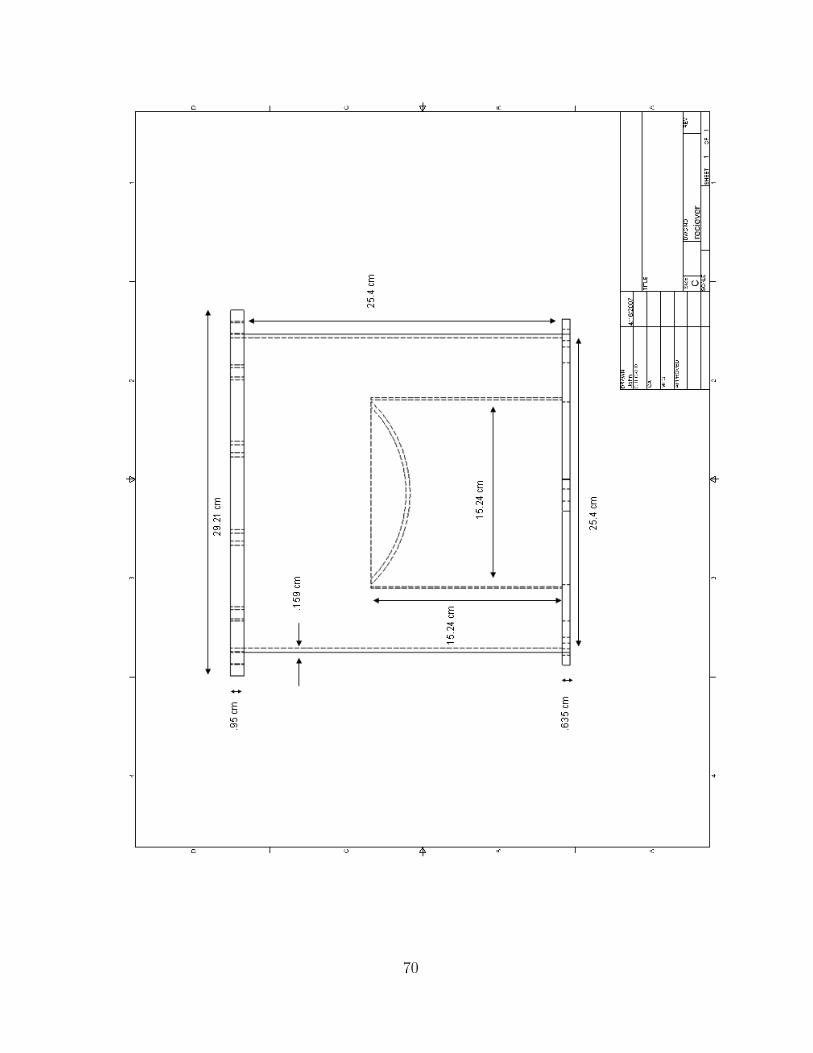
70
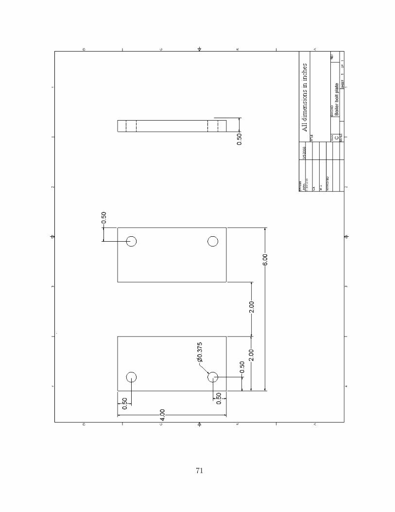
71
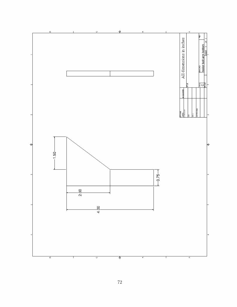
72

73

APPENDIX B
CONNECTION ARM DRAWINGS
74

75

76

APPENDIX C
CONCENTRATOR CONNECTION RING
DRAWINGS
77

78
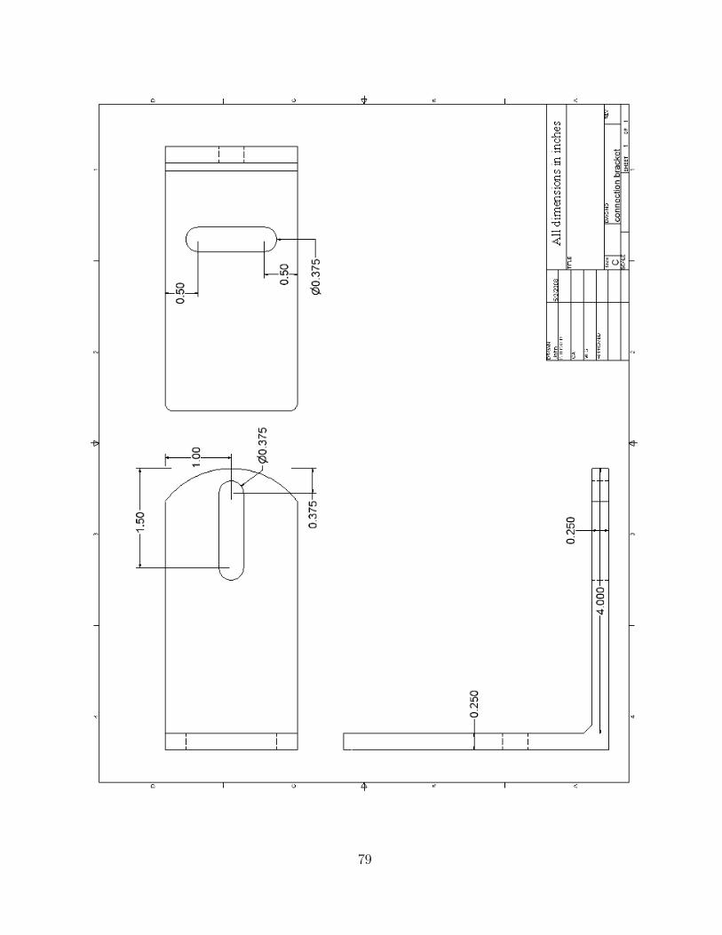
79

APPENDIX D
FOUNDATION DRAWINGS
80
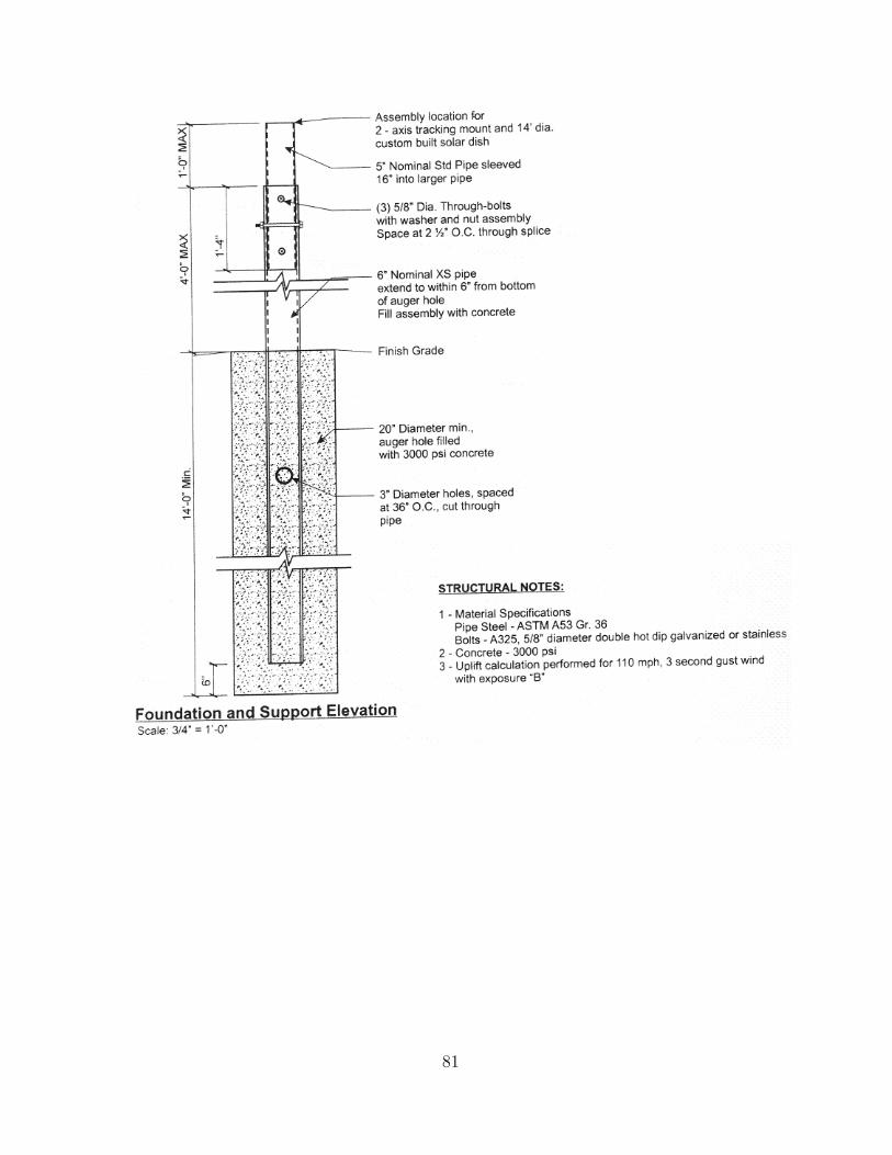
81

82
REFERENCES
[1] Dr. Anjaneyulu Krothapalli. Energy Conversion Systems. http ://sesec.fsu.edu/lectures.html, 2005. (document), 1.1
[2] Aden B Meinel and Marjorie P. Meilen. Applied Solar Energy, An Introduction. Addison-Wesley Publishing Company, Inc. Philippines, third edition edition, 1976. (document),1.2.1, 1.2, 1.2.1, 2.1, 2.12, 2.3.1, 2.18
[3] U.S. Department of Energy’s Sun∗Lab. http ://www.energylan.sandia.gov/sunlab/PDFs/boeing.pdf , August 2001. (document),1.3, 1.2.1
[4] W.B. Stine and R.W. Harrigan. Solar Energy System and Design, 1985. http ://www.powerfromthesun.net.htm. (document), 1.2.1, 1.2.2, 1.2.2, 1.4, 1.5, 1.6, 2.1
[5] The Nebraska Astronomy Applet Project. http ://astro.unl.edu/naap/motion3/siderealsynodic.html. (document), 2.5
[6] M. Eck and E. Zarza. Saturated steam process with direct steam generating parabolictroughs. Solar Energy, 80:1424–1433, 2006. (document), 1.7, 1.2.2
[7] Matt Anderson. Computer simulation of a solar dish power system for sustainable ruraldevelopment. Master’s thesis, Royal Institute of Technology, 2007. Page 42. (document),2.2, 2.3.3, 2.3.3, 2.4.4
[8] C. Christopher Newton. A concentrated solar thermal energy system. Master’s thesis,Florida State University, 2007. (document), 1.9, 1.10, 2.3, 2.17
[9] J.W. Spencer. Fourier series representation of the position of the sun. Journal of SolarEnergy, 1971. (document), 2.4
[10] Inc Wolverine Tube. Wolverine Engineering Data Book II. http ://www.wlv.com/products/databook/ch51.pdf , 2001. (document), 2.21
[11] Spirax Sarco USA. http : //www.spiraxsarco.com/resources/steam− engineering −tutorials/the− boiler − house/water − tube− boilers.asp. (document), 2.20
[12] Brenton Greska and Anjaneyulu Krothapalli. Tri-generation concentrating solar powersystem for rural applications. Technical Report ES2007-36169, Sustainable EnergyScience and Engineering Center, 2007. 1.1
83
[13] T. Mancini, P. Heller, B. Butler, B. Osborn, W. Schiel, V. Goldberg, R. Buck, R. Diver,C. Andraka, and J. Moreno. Dish-stirling systems: An overview of development andstatus. Journal of Solar Energy, 125:135–151, 2003. 1.1
[14] Richard B. Bannerot, John R. Howell, and Gary C. Vliet. Solar-Thermal EnergySystems, Analysis and Design. McGraw-Hill, Inc., 1982. 1.2.1, 2.1
[15] L.C. Spencer. A comprehensive review of small solar-powered heat engines: Part I. Ahistory of solar-powered devices up to 1950. Journal of Solar Energy, 43(4):191–196,1989. 1.2.1
[16] Robin M. Green. Spherical Astronomy. Cambridge University Press, 1985. 2.2.4
[17] Frank Kreith and Jan F. Kreider. Principles of Solar Engineering. HemispherePublishing Corporation, New York, 1978. 2.3.1
[18] John A Duffie and William A Beckman. Solar Engineering of Thermal Processes. JohnWiley & Sons, Inc., second edition, 1991. (document), 2.2, 2.8
[19] Donald Rapp. Solar Energy. Prentice-Hall, Inc. 1981. 2.3.1
[20] J. P. Holman. Heat Transfer. McGraw-Hill, ninth edition edition, 2002. 2.4.5
[21] Babcock & Wilcox Company. Steam, Its Generation and Use. Geo Mckibbin & Son,New York, 1955. 2.5.1
84

BIOGRAPHICAL SKETCH
John Dascomb
John Dascomb completed his Bachelors degree in Mechanical Engineering at Florida State
University in the Spring of 2006. Under the advisement of Prof. Anjaneyulu Krothapalli he
completed his Masters degree in the Spring of 2009.
John’s research interests include renewable energy, combustion, and heat transfer. He
will continue his studies under Dr. Krothapalli where he is currently enrolled in the doctoral
program.
85