Lossless coding for distributed streaming sources

Cheng Chang, Stark C. Draper, and Anant Sahai

October 18, 2006

Abstract

Distributed source coding is traditionally viewed in the block coding context — all the sourcesymbols are known in advance at the encoders. This paper instead considers a streaming settingin which iid source symbol pairs are revealed to the separate encoders in real time and need tobe reconstructed at the decoder with some tolerable end-to-end delay using finite rate noiselesschannels. A sequential random binning argument is used to derive a lower bound on the errorexponent with delay and show that both ML decoding and universal decoding achieve the samepositive error exponents inside the traditional Slepian-Wolf rate region. The error events aredifferent from the block-coding error events and give rise to slightly different exponents. Becausethe sequential random binning scheme is also universal over delays, the resulting code eventuallyreconstructs every source symbol correctly with probability 1.

1 Introduction

Traditionally, “lossless” coding is considered using two distinct paradigms: fixed block codingand variable-length coding1. As classically understood, both consider that the source-symbols areknown in advance at the encoder and that they must be mapped into a string of bits decoded bythe receiver. Fixed-block coding accepts a small probability of error and constrains the length ofthe bit-string, while variable-length encoding constrains only the expected length of the bit-string inexchange for keeping the probability of error at zero. In the point-to-point setting, both paradigmsapply generically. In contrast, distributed source coding, has traditionally been explored withinthe fixed block context. In [16], Slepian and Wolf even asked:

What is the theory of variable-length encodings for correlated sources?

In the classical context of source realizations known entirely in advance, the answer is simple:there is no nontrivial sense of variable-length encoding that applies generically while still beinginteresting.2 This is easiest to see by example (Illustrated in Figure 1 and revisited as Example 2 in

This material was presented in part at the IEEE Int Symp Inform Theory, Adelaide, Australia, Sept 2005.C. Chang is with the Department of Electrical Engineering and Computer Science, University of California

Berkeley, Berkeley, CA 94720 (E-mail: cchang@eecs.berkeley.edu).S. C. Draper is with Mitsubishi Electric Research Labs in Cambridge, MA. This work was performed while he was

a postdoc at Wireless Foundations in the University of California Berkeley (E-mail: sdraper@eecs.berkeley.edu).A. Sahai is with the Department of Electrical Engineering and Computer Science, University of California Berke-

ley, Berkeley, CA 94720 (E-mail: sahai@eecs.berkeley.edu).1There are actually four different traditional cases: fixed to fixed, fixed to variable, variable to fixed, and variable

to variable. However, the last three all achieve a probability of error of zero and so we consider them together.2At least at sum rates close to the joint source entropy rate. If the rates of communication are high enough, e.g.,

equaling the log of the cardinalities of the source alphabets, zero-error communication is possible.

1

Encoder y

Encoder x

Decoder3

Rx

s

Ry

-

-

-x1, x2, . . . , xN

y1, y2, . . . , yN

x1, x2, . . . , xN

y1, y2, . . . yN

(xi, yi) ∼ pxy

6

?

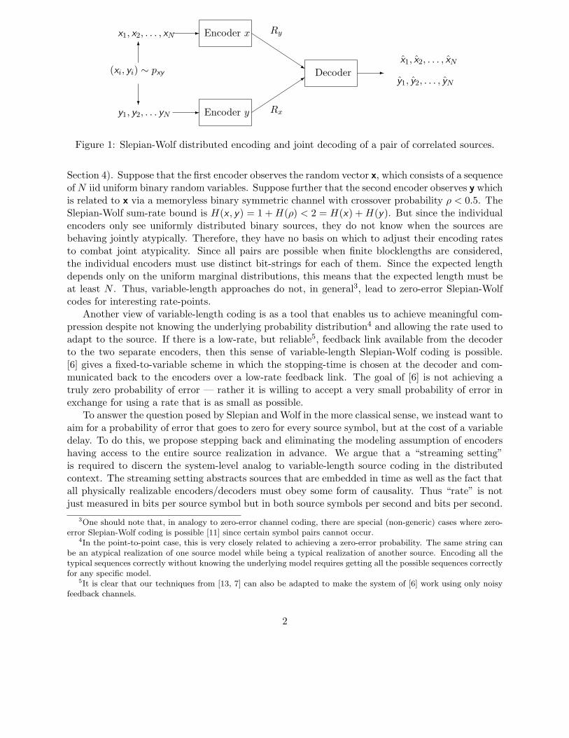
Figure 1: Slepian-Wolf distributed encoding and joint decoding of a pair of correlated sources.

Section 4). Suppose that the first encoder observes the random vector x, which consists of a sequenceof N iid uniform binary random variables. Suppose further that the second encoder observes y whichis related to x via a memoryless binary symmetric channel with crossover probability ρ < 0.5. TheSlepian-Wolf sum-rate bound is H(x , y) = 1 + H(ρ) < 2 = H(x) + H(y). But since the individualencoders only see uniformly distributed binary sources, they do not know when the sources arebehaving jointly atypically. Therefore, they have no basis on which to adjust their encoding ratesto combat joint atypicality. Since all pairs are possible when finite blocklengths are considered,the individual encoders must use distinct bit-strings for each of them. Since the expected lengthdepends only on the uniform marginal distributions, this means that the expected length must beat least N . Thus, variable-length approaches do not, in general3, lead to zero-error Slepian-Wolfcodes for interesting rate-points.

Another view of variable-length coding is as a tool that enables us to achieve meaningful com-pression despite not knowing the underlying probability distribution4 and allowing the rate used toadapt to the source. If there is a low-rate, but reliable5, feedback link available from the decoderto the two separate encoders, then this sense of variable-length Slepian-Wolf coding is possible.[6] gives a fixed-to-variable scheme in which the stopping-time is chosen at the decoder and com-municated back to the encoders over a low-rate feedback link. The goal of [6] is not achieving atruly zero probability of error — rather it is willing to accept a very small probability of error inexchange for using a rate that is as small as possible.

To answer the question posed by Slepian and Wolf in the more classical sense, we instead want toaim for a probability of error that goes to zero for every source symbol, but at the cost of a variabledelay. To do this, we propose stepping back and eliminating the modeling assumption of encodershaving access to the entire source realization in advance. We argue that a “streaming setting”is required to discern the system-level analog to variable-length source coding in the distributedcontext. The streaming setting abstracts sources that are embedded in time as well as the fact thatall physically realizable encoders/decoders must obey some form of causality. Thus “rate” is notjust measured in bits per source symbol but in both source symbols per second and bits per second.

3One should note that, in analogy to zero-error channel coding, there are special (non-generic) cases where zero-error Slepian-Wolf coding is possible [11] since certain symbol pairs cannot occur.

4In the point-to-point case, this is very closely related to achieving a zero-error probability. The same string canbe an atypical realization of one source model while being a typical realization of another source. Encoding all thetypical sequences correctly without knowing the underlying model requires getting all the possible sequences correctlyfor any specific model.

5It is clear that our techniques from [13, 7] can also be adapted to make the system of [6] work using only noisyfeedback channels.

2

The source-rate (symbols per second) is specified as a part of the problem while the bit-rate (bitsper second) is something that we get to choose. From an engineering perspective, three desirablequalities6 are:

• Using a low rate bit-pipe(s)

• Low end-to-end latency

• Low probability of error

The theory of source-coding should tell us the tradeoffs between these three desiderata. In addition,we will be interested in to what extent a streaming code can be made “universal” over a class ofprobability distributions.

In the point-to-point streaming setting, regardless of whether block or variable-length compres-sion is used, the traditional initial step is the same: group symbols into source blocks. To compressthe data blocks, either use a fixed-rate block code, or a variable-length code. The resulting en-coding is then enqueued for transmission across the bit-pipe. As long as the source entropy rateis below the data-rate, the queue will remain stable. When block coding is used for compression,there is a constant delay through the system, and atypical source blocks are received in error. Theprobability of error is fixed at the system’s design-time and so is the end-to-end delay.

In contrast, variable-length coding induces a variable system delay. The more unlikely thesource blocks, the longer the delay experienced at run-time. Thus, while asymptotically there areno errors when variable-length source codes are used (assuming an infinite buffer size), the delaytill a given symbol can be decoded depends on the random source realization. Because atypicalsource realizations are large deviation events, the probability that some source symbol cannot bereconstructed ∆ samples after it enters the encoder decays exponentially7 in ∆. The choice ofacceptable end-to-end delay is left to the receiver/application.

We show that this type of reliability can be achieved in a generic distributed coding context —the probability of error goes to zero with end-to-end delay and the choice of the acceptable delayis entirely up to the decoder. Essentially, every source symbol is recovered correctly eventuallywith probability8 1. The only difference is that unlike the point-to-point case, the decoder does notnecessarily know when the estimate for the symbol has converged to its final value. Furthermore,just as in the point-to-point setting9, both the encoding and decoding can be made universal.

In this paper, we formally define a streaming Slepian-Wolf code, and develop coding strategiesboth for situations when source statistics are known and when they are not. The new tool is asequential binning argument that parallels the tree-coding arguments used to study convolutionalcodes. We characterize the performance of the streaming schemes through an error exponentanalysis and demonstrate that the exponents are equal regardless of whether the system is informedof the source statistics (in which case we use maximum likelihood decoding) or not (in whichcase we use universal decoding). The universal decoder we design for the streaming problem is

6Of course, “implementation complexity” forms a fourth and very important consideration, but we will be ignoringthat aspect of the problem.

7In [2], we show that variable length codes used in this manner actually achieve the best possible error exponentwith delay. This is also related to the analysis of [10].

8The secret here is that we are considering a probability measure over infinite sequences. While all pairs of finitestrings may be possible, most pairs of infinite strings collectively have probability zero.

9Sliding-window Lempel-Ziv compression is one example where data is naturally encoded sequentially. It is alsouniversal over sources.

3

somewhat different from those familiar from the block coding literature, as are the nature of theerror exponents.

1.1 Potential applications and practical motivation

In addition to our core interest in answering some basic questions about Slepian-Wolf coding,our formulation is also motivated by the diverse emerging application areas for distributed sourcecoding. Media (e.g. video-conference) sources naturally have a streaming character. Consequently,we are motivated to explore what sort of streaming Slepian-Wolf technique matches naturally tosuch situations.10

1.2 Outline

Section 2 summarizes the notation used in the paper. Section 3 reviews the classical block-codingerror exponent results for Slepian-Wolf source coding and then we state the main results of thispaper: sequential error exponents for Slepian-Wolf source coding. Section 4 presents a numericstudy of two example sources. We observe that the sequential error exponent is often the same asthe block coding error exponent. Sections 5, 6 and 7 prove the theorems in Section 3. We start withsequential source coding for single sources in 5. This is the simplest case but it provides insightsto the nature of sequential source coding problem and sequential error events. We show that thesequential error exponent is the same as the random block source coding error exponent. Section 6moves on to the case with decoder side-information. Finally, Section 7 presents the proof of themain result of the paper. We derive the sequential error exponent of distributed source codingfor correlated sources. This error exponent strictly positive everywhere inside the achievable rateregion of [16]. For all these three scenarios in Sections 5, 6 and 7, both ML and universal decodingrules are studied. The appendix shows that the resulting error exponents are indeed the same.

2 Notation

We use serifed-fonts, e.g., x to indicate sample values, and sans-serif, e.g., x , to indicate randomvariables. Bolded fonts are reserved to indicate sample or random vectors, e.g., x = xn and x = x

n,respectively, where the vector length (n here) is understood from the context. Subsequences, e.g.,xl, xl+1, . . . , xn are denoted as xn

l where xji , ∅ if i < j. Distributions are indicated with lower-case

p, e.g., x is distributed according to px(x). Sets and their elements are denoted as, e.g., x ∈ X , andtheir cardinality by |X |. We use calligraphic font to denote sets, X , F , W etc, and reserve E and D todenote encoding and decoding functions, respectively. We use standard notation for types, see, e.g.,[5]. Let N(a;x) denote the number of symbols in the length-n vector x that take on value a. Then,x is of type P if P (a) = N(a;x)/n. The type-class, or set of length-n vectors of type P is denotedTP . A sequence y has conditional type V given x if N(a, b;x,y) = N(a;x)V (b|a) = P (a)V (b|a) forevery a, b. The set of sequences y having conditional type V with respect to x is called the V -shellof x and is denoted by TV (x). When considered together, the pair (x,y) is said to have joint type

10A secondary aspect in some multimedia settings is a natural multi-scale nature to the source — the high orderbits are more important than the low order bits. To the extent that the high order bits can be made “early” and thelow-order bits can be made “late”, our constructions also naturally give more protection to the early bits as comparedto the later ones. While this interpretation might eventually be important in practice, it is a bit questionable withinthe simplified model this paper considers.

4

V × P . We always use upper-case, e.g., P and V , to denote length-n types and conditional types.As we often discuss the types of subsequences we add a superscript notation to remind the readerof the length of the subsequence in question. If, for instance, the subsequence under considerationis xn

l we write xnl ∈ TP n−l . Similarly we use V n−l for the conditional type of length-(n− l +1), and

V n−l × Pn−l for the joint type. Given a joint type V × P , entropies and conditional entropies aredenoted as H(P ) and H(V |P ), respectively. The KL divergence between two distributions q and pis denoted by D(q‖p).

3 Main Results

In this section, we begin by reviewing classical results on the error exponents of distributed blockcoding. We then present the main results of the paper: error exponents for streaming Slepian-Wolfcoding and its special cases: point-to-point coding and source coding with decoder side information.We analyze both maximum likelihood and universal decoding and show that the achieved exponentsare equal. Leaving numerical examples and proofs for later sections, we here compare the form ofthe streaming exponents with their block coding counterparts.

3.1 Block source coding and error exponents

In the classic block-coding Slepian-Wolf paradigm, full length-N vectors x and y are observedby their respective encoders before communication commences. In this situation a rate-(Rx, Ry)length-N block source code consists of an encoder-decoder triplet (Ex

N , EyN ,DN ), as we will define

shortly. For the rate-region considerations, the general case of distributed encoders can be con-sidered by using time-sharing among codes that alternate between sending at rates close to themarginal entropy and those that correspond to perfectly known side-information. However, it iseasy to see that this results in a substantial loss of error-exponent even in the block-coding case.To get good exponents, something else is required:

Definition 1 A randomized length-N rate-(Rx, Ry) block encoder-decoder triplet (ExN , Ey

N ,DN ) isa set of maps

ExN : XN → {0, 1}NRx , e.g., Ex

N (xN ) = aNRx

EyN : YN → {0, 1}NRy , e.g., Ey

N (yN ) = bNRy

DN : {0, 1}NRx × {0, 1}NRy → X n × Yn, e.g., DN (aNRx , bNRy) = (xN , yN )

where common randomness, shared between the encoders and the decoder is assumed. This allowsus to randomize the mappings independently of the source sequences.

The error probability typically considered in Slepian-Wolf coding is the joint error probability,Pr[(xN , yN ) 6= (xN , yN )] = Pr[(xN , yN ) 6= DN (Ex

N (xN ), EyN (yN ))]. This probability is taken over

the random source vectors as well as the randomized mappings. An error exponent E is said to beachievable if there exists a family of rate-(Rx, Ry) encoders and decoders {(Ex

N , EyN ,DN )}, indexed

by N , such that

limN→∞

−1

Nlog Pr[(xN , yN ) 6= (xN , yN )] ≥ E. (1)

5

In this paper, we study random source vectors (x, y) that are iid across time but may havedependencies at any given time:

px ,y (x,y) =

N∏

i=1

px ,y (xi, yi).

For such iid sources, upper and lower bounds on the achievable error exponents are derivedin [9, 5]. These results are summarized by the following theorem.

Theorem 1 (Lower bound) Given a rate pair (Rx, Ry) such that Rx > H(x |y), Ry > H(y |x),Rx + Ry > H(x , y). Then, for all

E < minx ,y

D(px ,y‖pxy ) +∣

∣min[Rx + Ry − H(x , y), Rx − H(x |y), Ry − H(y |x)]∣

∣

+(2)

there exists a family of randomized encoder-decoder mappings as defined in Definition 1 such that (1)is satisfied. In (2) the function |z|+ = z if z ≥ 0 and |z|+ = 0 if z < 0.

(Upper bound) Given a rate pair (Rx, Ry) such that Rx > H(x |y), Ry > H(y |x), Rx + Ry >H(x , y). Then, for all

E > min

{

minx ,y :Rx<H(x |y)

D(px ,y‖pxy ), minx ,y :Ry<H(y |x)

D(px ,y‖pxy ), minx ,y :Rx+Ry<H(x ,y)

D(px ,y‖pxy )

}

(3)

there does not exists a randomized encoder-decoder mapping as defined in Definition 1 such that (1)is satisfied.

In both bounds (x , y) are dummy random variables with joint distribution px ,y .

Remark: As long as (Rx, Ry) is in the interior of the achievable region, i.e., Rx > H(x |y),Ry > H(y |x) and Rx +Ry > H(x , y) then the lower-bound (2) is positive. The achievable region isillustrated in Fig 2. As shown in [5], the upper and lower bounds (3) and (2) match when the ratepair (Rx, Ry) is achievable and close to the boundary of the region. This is analogous to the highrate regime in channel coding where the random coding bound (analogous to (2)) and the spherepacking bound (analogous to (3)) agree.

Theorem 1 can also be used to generate bounds on the exponent for source coding with decoderside information (i.e., y observed at the decoder), and for source coding without side information(i.e., y is a constant). These corollaries will prove useful as a basis for comparison as we build upto the complete solution for streaming Slepian-Wolf coding.

Corollary 1 (Source coding with decoder side information) Consider a Slepian-Wolf problem wherey is known by the decoder. Given a rate Rx such that Rx > H(x |y), then for all

E < minx ,y

D(px ,y‖pxy ) + |Rx − H(x |y)|+, (4)

there exists a family of randomized encoder-decoder mappings as defined in Definition 1 such that (1)is satisfied.

The proof of Corollary 1 follows from Theorem 1 by letting Ry be arbitrarily large. Similarly, byletting y be deterministic so that H(x |y) = H(x) and H(y) = 0, we get the following random-codingbound for the point-to-point case of a single source x.

6

Corollary 2 (point-to-point) Consider a Slepian-Wolf problem where y is deterministic, i.e., y =y. Given a rate Rx such that Rx > H(x), for all

E < minx

D(px‖px) + |Rx − H(x)|+ = Ex(Rx) (5)

there exists a family of randomized encoder-decoder triplet as defined in Definition 1 such that (1)is satisfied.

-

6

Ry

Rx

H(y)

H(y |x)

H(x)H(x |y)

log |Y|

log |X |

AchievableRegion

Rx + Ry = H(x , y)

�

Figure 2: Achievable region for Slepian-Wolf source coding

3.2 Sequential Distributed Source Coding

We now state our main results for streaming encoding, and contrast them with the block-codingresults of the last section. To begin, we define a streaming encoder.

Definition 2 A randomized sequential encoder-decoder triplet Ex, Ey,D is a sequence of mappings,{Ex

j }, j = 1, 2, ..., {Eyj }, j = 1, 2, ... and {Dj}, j = 1, 2, ...:

Exj : X j −→ {0, 1}Rx , e.g., Ex

j (xj) = ajRx

(j−1)Rx+1,

Eyj : Yj −→ {0, 1}Ry , e.g., Ey

j (yj) = bjRy

(j−1)Ry+1.(6)

Common randomness, shared between encoders and decoder, is assumed. This allows us to ran-domize the mappings independently of the source sequence.

In this paper, the sequential encoding maps will always work by assigning random “parity bits”in a causal manner to the observed source sequence. That is, the Rx (or Ry) bits generated at each

7

time in (6), are iid Bernoulli-(0.5).11 Since parity bits are assigned causally, if two source sequencesshare the same length-l prefix, then their first lRx parity bits must match. Subsequent parities aredrawn independently. Such a sequential coding strategy is the source-coding parallel to tree andconvolutional codes used for channel coding [8]. In fact, we call these “parity bits” as they can begenerated using an infinite constraint-length time-varying random convolutional code.

Definition 3 The decoder mapping

Dj : {0, 1}jRx × {0, 1}jRy −→ X j × Yj

Dj(ajRx , bjRy) = (xj

1(j), yj1(j))

At each time j the decoder Dj outputs estimates of all the source symbols that have entered theencoder by time j.

Remark: While we state Definition 2 only for Slepian-Wolf coding, it immediately specializesto source coding with decoder side information (dropping the Ey and revealing y

n to the decoder),and source coding without side information (dropping the Ey). We present results for both thesesituations as well.

In this paper we study two error probabilities. We define the pair of source estimates at time nas (xn, yn) = Dn(

∏nj=1 E

xj ,∏n

j=1 Eyj ), where

∏nj=1 E

xj indicates the full nRx bit stream from encoder

x up to time n. We use (xn−∆, yn−∆) to indicate the first n − ∆ symbols of each estimate, wherefor conciseness of notation both the estimate time, n, and the decoding delay, ∆, are indicated inthe superscript. With these definitions the two error probabilities we study are

Pr[xn−∆ 6= xn−∆] and Pr[yn−∆ 6= y

n−∆].

A pair of exponents Ex > 0 and Ey > 0 is said to be achievable if there exists a family of rate-(Rx, Ry) encoders and decoders {(Ex

j , Eyj ,Dj)} such that

lim∆→∞

limn→∞

−1

∆log Pr[xn−∆ 6= x

n−∆] ≥ Ex (7)

lim∆→∞

limn→∞

−1

∆log Pr[yn−∆ 6= y

n−∆] ≥ Ey (8)

Remarks: In contrast to (1) the error exponent we look at is in the delay, ∆, rather than totalobservation time, n. The order of the limits is important since the total time-period n is allowedto go to infinity faster than the delay ∆. While the definitions of (7)–(8) and of (1) are asymptoticin nature, the results hold for finite block-lengths and delays as well. Finally, we note that whilein (1) the error exponent of a joint error event on either x or y is considered, we provide a refined

11We assume that Rx and Ry are integer. To justify this assumption note that we can always group sets of αsuccessive symbols into super-symbols. These larger symbols can be encoded at an average rate αRx. Generally,if we group α symbols together, and transmit β bits per super-symbol, we can realize an average rate α/β, i.e., arational rate. If desired, non-integer average rates are easily implemented by a time-varying transmission rate. Forexample, say we want to implement an average encoding rate of 5/4 bits per source symbol. Say we generate one newparity bit per symbol for each symbol observed except for the fourth symbol, eighth symbol, etc, when we generatetwo. The average encoding rate is 5/4. As long as the decoding delay ∆ we target is long enough so that the decoderreceived an “average” number of encoded bits – δRx – before we must make an estimate (e.g., if ∆ ≫ 1/Rx), thesesmall-scale issues even out. In particular, they do not effect the exponents.

8

analysis specifying potentially different exponents on either decision. The results for joint errorsare found by taking the minimum of the individual exponents, i.e.,

lim∆→∞

limn→∞

−1

∆log Pr[(xn−∆, yn−∆) 6= (xn−∆, yn−∆)] ≥ min{Ex, Ey}.

3.3 Streaming source coding

Our first results concern streaming coding in the point-to-point setting. The first theorem we stategives random coding error exponents for maximum likelihood decoding where the source statisticsare known, and the second exponents for universal decoding, where they are not.

Theorem 2 Given a rate Rx > H(px), there exists a randomized streaming encoder and maximumlikelihood decoder pair (per Definition 2) such that for all E < EML(Rx) there is a constant K > 0such that Pr[xn−∆ 6= x

n−∆] ≤ K exp{−∆EML(Rx)} for all n, ∆ ≥ 0 where

EML(Rx) = sup0≤ρ≤1

ρRx − (1 + ρ) log

(

∑

x

px(x)1

1+ρ

)

. (9)

Theorem 3 Given a rate Rx > H(px), there exists a randomized streaming encoder and universaldecoder pair (per Definition 2) such that for all E < EUN (Rx) there is a constant K > 0 such thatPr[xn−∆ 6= x

n−∆] ≤ K exp{−∆E} for all n, ∆ ≥ 0 where

EUN (Rx) = infq

D(q‖px) + |Rx − H(q)|+, (10)

where q is an arbitrary probability distribution on X and where |z|+ = z if z ≥ 0 and |z|+ = 0 ifz < 0.

Remark: The error exponents of Theorems 2 and 3 both equal their respective random block-coding exponents for ML and universal decoders. For example, compare (10) with (5). The maindifference in the formulation is that the error probability decays with delay ∆ rather than blocklength N . Furthermore, it is known that (9) and (10) are equal — see [5] exercise 13 on page 44.Such equality is required by the formal definition of a universal scheme, i.e., for the same sourcestatistics and coding rates, the universal decoder should asymptotically achieve the same errorexponent as the maximum likelihood decoder. See [12] for a detailed discussion of universal versusmaximum likelihood decoding in the context of channel coding.

3.4 Streaming distributed source coding with decoder side information

This section summarizes our results for distributed streaming source coding when the side infor-mation is observed at the decoder, but not the encoder:

Theorem 4 Given a rate Rx > H(x |y), there exists a randomized encoder decoder pair (per Defi-nition 2) such that for all E < EML,SI(Rx) there is a constant K > 0 such that Pr[xn−∆ 6= x

n−∆] ≤K exp{−∆E} for all n, ∆ ≥ 0 where

EML,SI(Rx) = sup0≤ρ≤1

ρRx − log[

∑

y

[

∑

x

pxy (x, y)1

1+ρ

]1+ρ]

. (11)

9

Theorem 5 Given a rate Rx > H(x |y), there exists a randomized encoder decoder pair (per Def-inition 2 ) such that for all E < EUN,SI(Rx) there is a constant K > 0 such that Pr[xn−∆ 6=x

n−∆] ≤ K exp{−∆E} for all n, ∆ ≥ 0 where

EUN,SI(Rx) = infx ,y

D(px ,y‖pxy ) + |Rx − H(x |y)|+, (12)

and (x , y) are random variables with joint distribution px ,y , H(x |y) is their conditional entropy,and where |z|+ = z if z ≥ 0 and |z|+ = 0 if z < 0.

Remark: Similar to the point-to-point case, the error exponents of Theorems 4 and 5 both equaltheir respective random block-coding exponents. For example, compare (12) with (4). Similarly,(11) and (12) can be shown to be equal.

3.5 Streaming Slepian-Wolf coding

In contrast to streaming point-to-point coding and streaming source coding with decoder sideinformation, the general case of streaming Slepian-Wolf coding with two distributed encoders resultsin error exponents that differ from their block coding counterparts. In the streaming setting,fundamentally different error events dominate as compared to the block setting.

Theorem 6 Let (Rx, Ry) be a rate pair such that Rx > H(x |y), Ry > H(y |x), Rx +Ry > H(x , y).Then, there exists a randomized encoder pair and maximum likelihood decoder triplet (per Defini-tion 2) that satisfies the following three decoding criteria.

(i) For all E < EML,SW,x(Rx, Ry), there is a constant K > 0 such that Pr[xn−∆ 6= xn−∆] ≤

K exp{−∆E} for all n, ∆ ≥ 0 where

EML,SW,x(Rx, Ry) = min

{

infγ∈[0,1]

EMLx (Rx, Ry, γ), inf

γ∈[0,1]

1

1 − γEML

y (Rx, Ry, γ)

}

.

(ii) For all E < EML,SW,y(Rx, Ry) there is a constant K > 0 such that Pr[yn−∆ 6= yn−∆] ≤

K exp{−∆E} for all n, ∆ ≥ 0 where

EML,SW,y(Rx, Ry) = min

{

infγ∈[0,1]

1

1 − γEML

x (Rx, Ry, γ), infγ∈[0,1]

EMLy (Rx, Ry, γ)

}

.

(iii) For all E < EML,SW,xy(Rx, Ry) there is a constant K > 0 such that Pr[(xn−∆, yn−∆) 6=(xn−∆, yn−∆)] ≤ K exp{−∆E} for all n, ∆ ≥ 0 where

EML,SW,xy(Rx, Ry) = min

{

infγ∈[0,1]

EMLx (Rx, Ry, γ), inf

γ∈[0,1]EML

y (Rx, Ry, γ)

}

.

In definitions (i)–(iii),

EMLx (Rx, Ry, γ) = supρ∈[0,1][γEx|y(Rx, ρ) + (1 − γ)Exy(Rx, Ry, ρ)]

EMLy (Rx, Ry, γ) = supρ∈[0,1][γEy|x(Rx, ρ) + (1 − γ)Exy(Rx, Ry, ρ)]

(13)

10

and

Exy(Rx, Ry, ρ) = ρ(Rx + Ry) − log[

∑

x,y pxy (x, y)1

1+ρ

]1+ρ

Ex|y(Rx, ρ) = ρRx − log[

∑

y

[

∑

x pxy (x, y)1

1+ρ

]1+ρ]

Ey|x(Ry, ρ) = ρRy − log[

∑

x

[

∑

y pxy (x, y)1

1+ρ

]1+ρ]

(14)

Theorem 7 Let (Rx, Ry) be a rate pair such that Rx > H(x |y), Ry > H(y |x), Rx +Ry > H(x , y).Then, there exists a randomized encoder pair and universal decoder triplet (per Definition 2) thatsatisfies the following three decoding criteria.

(i) For all E < EUN,SW,x(Rx, Ry), there is a constant K > 0 such that Pr[xn−∆ 6= xn−∆] ≤

K exp{−∆E} for all n, ∆ ≥ 0 where

EUN,SW,x(Rx, Ry) = min

{

infγ∈[0,1]

EUNx (Rx, Ry, γ), inf

γ∈[0,1]

1

1 − γEUN

y (Rx, Ry, γ)

}

. (15)

(ii) For all E < EUN,SW,y(Rx, Ry), there is a constant K > 0 such that Pr[yn−∆ 6= yn−∆] ≤

K exp{−∆E} for all n, ∆ ≥ 0 where

EUN,SW,y(Rx, Ry) = min

{

infγ∈[0,1]

1

1 − γEUN

x (Rx, Ry, γ), infγ∈[0,1]

EUNy (Rx, Ry, γ)

}

. (16)

(iii) For all E < EUN,SW,xy(Rx, Ry), there is a constant K > 0 such that Pr[(xn−∆, xn−∆) 6=(xn−∆, yn−∆)] ≤ K exp{−∆E} for all n, ∆ ≥ 0 where

EUN,SW,xy(Rx, Ry) = min

{

infγ∈[0,1]

EUNx (Rx, Ry, γ), inf

γ∈[0,1]EUN

y (Rx, Ry, γ)

}

. (17)

In definitions (i)–(iii),

EUNx (Rx, Ry, γ) = inf

x ,y ,x ,yγD(px ,y‖pxy ) + (1 − γ)D(px ,y‖pxy ) + |γ[Rx − H(x |y)] + (1 − γ)[Rx + Ry − H(x , y)]|+

EUNy (Rx, Ry, γ) = inf

x ,y ,x ,yγD(px ,y‖pxy ) + (1 − γ)D(px ,y‖pxy ) + |γ[Ry − H(y |x)] + (1 − γ)[Rx + Ry − H(x , y)]|+

(18)

where the random variables (x , y) and (x , y) have joint distributions px ,y and px ,y , respectively. Thefunction |z|+ = z if z ≥ 0 and |z|+ = 0 if z < 0.

Remark: Definitions (i) and (ii) in Theorems 6 and 7 concern individual decoding error eventswhich might be useful in applications where the x and y streams are decoded jointly, but utilizedindividually. The more standard joint error event is given by (iii).

Remark: We can compare the joint error event for block and streaming Slepian-Wolf coding,c.f. (17) with (2). The streaming exponent differs by the extra parameter γ that must be minimizedover. If the minimizing γ = 1, then the block and streaming exponents are the same. Theminimization over γ results from a fundamental difference in the types of error-causing events thatcan occur in streaming Slepian-Wolf as compared to block Slepian-Wolf.

Remark: The error exponents of maximum likelihood and universal decoding in Theorems 6and 7 are the same. However, because there are new classes of error events possible in streaming,this needs proof. The equivalence is summarized in the following theorem.

11

Theorem 8 Let (Rx, Rx) be a rate pair such that Rx > H(x |y), Ry > H(y |x), and Rx + Ry >H(x , y). Then,

EML,SW,x(Rx, Ry) = EUN,SW,x(Rx, Ry), (19)

andEML,SW,x(Rx, Ry) = EUN,SW,x(Rx, Ry). (20)

Theorem 8 follows directly from the following lemma, shown in the appendix.

Lemma 1 For all γ ∈ [0, 1]

EMLx (Rx, Ry, γ) = EUN

x (Rx, Ry, γ), (21)

andEML

y (Rx, Ry, γ) = EUNy (Rx, Ry, γ). (22)

.

Remark: This theorem allows us to simplify notation. For example, we can define Ex(Rx, Ry, γ)as Ex(Rx, Ry, γ) = EML

x (Rx, Ry, γ) = EUNx (Rx, Ry, γ), and can similarly define Ey(Rx, Ry, γ). Fur-

ther, since the ML and universal exponents are the same for the whole rate region we can defineESW,x(Rx, Ry) as ESW,x(Rx, Ry) = EML,SW,x(Rx, Ry) = EUN,SW,x(Rx, Ry), and can similarly de-fine ESW,y(Rx, Ry).

4 Numerical Results

To build insight into the differences between the sequential error exponents of Theorem 2 - 8 andblock-coding error exponents, we give some examples of the exponents for binary sources.

For the point-to-point case, the error exponents of random sequential and block source codingare identical everywhere in the achievable rate region as can be seen by comparing Theorem 3 andCorollary 2. The same is true for source coding with decoder side information (cf. Theorem 5 andCorollary 1). For distributed Slepian-Wolf source coding however, the sequential and block errorexponents can be different. The reason for the discrepancy is that a new type of error event can bedominant in Slepian-Wolf source coding. This is reflected in Theorem 6 by the minimization overγ. Example 2 illustrates the impact of this γ term.

For Slepian-Wolf source coding at very high rates, where Rx > H(x), the decoder can ignoreany information from encoder y and still decode x with with a positive error exponent. However,the decoder could also choose to decode source x and y jointly. Fig 6.a and 6.b illustrate thatjoint decoding may or surprisingly may not help decoding source x. This is seen by comparing theerror exponent when the decoder ignores the side information from encoder y (the dotted curves)to the joint error exponent (the lower solid curves). It seems that when the rate for source y is low,atypical behaviors of source y can cause joint decoding errors that end up corrupting x estimates.This holds for both block and sequential coding.

12

-

6

Ry

Rx

. . . . . . . . . . . . . . . . . . . . . . . . .0.49

. . . . . . . . . . . . . . . . . . . . . . . . .0.67

AchievableRegion

Rx + Ry = H(x , y)

�

Figure 3: Rate region for the example 1 source, we focus on the error exponent on source x forfixed encoder y rates: Ry = 0.49 and Ry = 0.67

4.1 Example 1: symmetric source with uniform marginals

Consider a symmetric source where |X | = |Y| = 2, pxy (0, 0) = 0.45, pxy (0, 1) = pxy (1, 0) = 0.05and pxy (1, 1) = 0.45. This is a marginally-uniform source: x is Bernoulli(1/2), y is the outputfrom a BSC with input x , thus y is Bernoulli(1/2) as well. For this source H(x) = H(y) = log(2),H(x |y) = H(y |x) = 0.32, H(x , y) = 1.02. The achievable rate region is the triangle shown inFigure(3).

For this source, as will be shown later, the dominant sequential error event is on the diagonalline in Fig 9. This is to say that:

ESW,x(Rx, Ry) = EBLOCKSW,x (Rx, Ry) = EML

x (Rx, Ry, 0) = supρ∈[0,1]

[Exy(Rx, Ry, ρ)]. (23)

Where EBLOCKSW,x (Rx, Ry) = min{EML

x (Rx, Ry, 0), EMLx (Rx, Ry, 1)} as shown in [9].

Similarly for source y:

ESW,y(Rx, Ry) = EBLOCKSW,y (Rx, Ry) = EML

y (Rx, Ry, 0) = supρ∈[0,1]

[Exy(Rx, Ry, ρ)]. (24)

13

We first show that for this source ∀ρ ≥ 0, Ex|y(Rx, ρ) ≥ Exy(Rx, Ry, ρ). By definition:

Ex|y(Rx, ρ) − Exy(Rx, Ry, ρ) = ρRx − log[

∑

y

[

∑

x

pxy (x, y)1

1+ρ

]1+ρ]

−(

ρ(Rx + Ry) − log[

∑

x,y

pxy (x, y)1

1+ρ

]1+ρ)

= −ρRy − log[

2[

∑

x

pxy (x, 0)1

1+ρ

]1+ρ]

+ log[

2∑

x

pxy (x, 0)1

1+ρ

]1+ρ

= −ρRy − log[

2]

+ log[

2]1+ρ

= ρ(log[2] − Ry)

≥ 0

The last inequality is true because we only consider the problem when Ry ≤ log |Y|. Otherwise,y is better viewed as perfectly known side-information. Now

EMLx (Rx, Ry, γ) = sup

ρ∈[0,1][γEx|y(Rx, ρ) + (1 − γ)Exy(Rx, Ry, ρ)]

≥ supρ∈[0,1]

[Exy(Rx, Ry, ρ)]

= EMLx (Rx, Ry, 0)

Similarly EMLy (Rx, Ry, γ) ≥ EML

y (Rx, Ry, 0) = EMLx (Rx, Ry, 0). Finally,

ESW,x(Rx, Ry) = min

{

infγ∈[0,1]

Ex(Rx, Ry, γ), infγ∈[0,1]

1

1 − γEy(Rx, Ry, γ)

}

= EMLx (Rx, Ry, 0)

Particularly Ex(Rx, Ry, 1) ≥ Ex(Rx, Ry, 0), so

EBLOCKSW,x (Rx, Ry) = min{EML

x (Rx, Ry, 0), EMLx (Rx, Ry, 1)}

= EMLx (Rx, Ry, 0)

The same proof holds for source y.In Fig 4 we plot the joint sequential/block coding error exponents ESW,x(Rx, Ry) = EBLOCK

SW,x (Rx, Ry),the error exponents are positive iff Rx > H(xy) − Ry = 1.02 − Ry.

4.2 Example 2: non-symmetric source

Consider a non-symmetric source where |X | = |Y| = 2, pxy (0, 0) = 0.1, pxy (0, 1) = pxy (1, 0) =0.05 and pxy (1, 1) = 0.8. For this source H(x) = H(y) = 0.42, H(x |y) = H(y |x) = 0.29 andH(x , y) = 0.71. The achievable rate region is shown in Fig 5. In Fig 6.a, 6.b, 6.c and 6.d, wecompare the joint sequential error exponent ESW,x(Rx, Ry) the joint block coding error exponentEBLOCK

SW,x (Rx, Ry) = min{Ex(Rx, Ry, 0), Ex(Rx, Ry, 1)} as shown in [9] and the individual error

14

0 0.35 0.53 log(2)0

0.05

0.1

0.15

0.2

0.25

Err

or e

xpon

ent f

or s

ourc

e x

Rate of encoder x

R =0.67

R =0.49

y

y

Figure 4: Error exponents plot: ESW,x(Rx, Ry) plotted for Ry = 0.49 and Ry = 0.67ESW,x(Rx, Ry) = EBLOCK

SW,x (Rx, Ry) = ESW,y(Rx, Ry) = EBLOCKSW,y (Rx, Ry) and Ex(Rx) = 0

exponent for source X, Ex(Rx) as shown in Corollary 2. Notice that Ex(Rx) > 0 only if Rx > H(x).In Fig 7, we compare the sequential error exponent for source y: ESW,y(Rx, Ry) and the blockcoding error exponent for source y: EBLOCK

SW,y (Rx, Ry) = min{Ey(Rx, Ry, 0), Ey(Rx, Ry, 1)} andEy(Ry) which is a constant since we fix Ry.

For Ry = 0.35 as shown in Fig 6.a.b and 7.a.b, the difference between the block coding andsequential coding error exponents is very small for both source x and y. More interestingly, asshown in Fig 6.a, because the rate of source y is low, i.e. it is more likely to get a decoding errordue to the atypical behavior of source y. So as Rx increases, it is sometimes better to ignore sourcey and decode x individually. This is evident as the dotted curve is above the solid curves.

For Ry = 0.49 as shown in Fig 6.c.d and 7.c.d, since the rate for source y is high enough, sourcey can be decoded with a positive error exponent individually as shown in Fig 7.c. But as the rateof source x increases, joint decoding gives a better error exponent. When Rx is very high, then weobserve the saturation of the error exponent on y as if source x is known perfectly to the decoder!This is illustrated by the flat part of the solid curves in Fig 7.c.

5 Streaming point-to-point coding via sequential random binning

In this section we prove Theorems 2 and 3. While the emphasis of the paper is on distributedsource coding, the basic causal random binning ideas and analysis techniques can be more easilydeveloped in the point-to-point context.

15

-

6

Ry

Rx

. . . . . . . . . . . . . . . . . . . . . . . . .

. . . . . . . . . . . . . . . . . . . . . . . . .

0.35

0.49

AchievableRegion

Rx + Ry = H(x , y)

�

Figure 5: Rate region for the example 2 source, we focus on the error exponent on source x forfixed encoder y rates: Ry = 0.35 and Ry = 0.49

5.1 Maximum-likelihood decoding

To show Theorems 2 and 3, we first develop the common core of the proof in the context of MLdecoding. The proof strategy is as follows. A decoding error can only occur if there is somespurious source sequence xn that satisfies three conditions: (i) it must be in the same bin (sharethe same parities) as xn, i.e., xn ∈ Bx(xn), (ii) it must be more likely than the true sequence, i.e.,px(x

n) > px(xn), and (iii) xl 6= xl for some l ≤ n − ∆.

The error probability is

Pr[xn−∆ 6= xn−∆] =

∑

xn

Pr[xn−∆ 6= xn−∆|xn = xn]px(xn) (25)

=∑

xn

n−∆∑

l=1

Pr[

∃ xn ∈ Bx(xn) ∩ Fn(l, xn) s.t. px(xn) ≥ px(x

n)]

px(xn) (26)

=n−∆∑

l=1

{

∑

xn

Pr[

∃ xn ∈ Bx(xn) ∩ Fn(l, xn) s.t. px(xn) ≥ px(x

n)]

px(xn)}

=n−∆∑

l=1

pn(l). (27)

After conditioning on the realized source sequence in (25), the remaining randomness is only inthe binning. In (26) we decompose the error event into a number of mutually exclusive events (seeFig 8) by partitioning all source sequences xn into sets Fn(l, xn) defined by the time l of the firstsample in which they differ from the realized source xn,

Fn(l, xn) = {xn ∈ X n|xl−1 = xl−1, xl 6= xl}, (28)

16

0 0.36 log(2) 0

0.05

0.1

0.15

0.2

(a)

R = 0.35

0 log(2)0

0.1

0.2

0.3

0.4

0.5

(b)

0 0.29 0.42 log(2)0

0.05

0.1

0.15

0.2

(c)

0 log(2)0

0.1

0.2

0.3

0.4

0.5

(d)

R

x

R

x

R

x

R

x

y R = 0.49

y

Figure 6: Error exponents plot for source x for fixed Ry as Rx varies:Ry = 0.35:(a) Solid curve: ESW,x(Rx, Ry), dashed curve EBLOCK

SW,x (Rx, Ry) and dotted curve: Ex(Rx), notice

that ESW,x(Rx, Ry) ≤ EBLOCKSW,x (Rx, Ry) but the difference is small.

(b) 10 log10(EBLOCK

SW,x (Rx,Ry)

ESW,x(Rx,Ry) ). This shows the difference is there at high rates.

Ry = 0.49:(c) Solid curve ESW,x(Rx, Ry), dashed curve EBLOCK

SW,x (Rx, Ry) and dotted curve: Ex(Rx), again

ESW,x(Rx, Ry) ≤ EBLOCKSW,x (Rx, Ry) but the difference is extremely small.

(d) 10 log10(EBLOCK

SW,x (Rx,Ry)

ESW,x(Rx,Ry) ). This shows the difference is there at intermediate low rates.

17

0 0.36 log(2)0

0.01

0.02

0.03

0.04

0.05

0.06

(a)

R = 0.35

0 log(2)0

0.05

0.1

0.15

0.2

0.25

(b)

0 0.29 log(2)0

0.01

0.02

0.03

0.04

0.05

0.06

(c)

R = 0.49

log(2)0

0.05

0.1

0.15

0.2

0.25

R

x

R

x

R

x

R

x

infinity

y y

E (R )

ML y

E (R ) ML y

(d)

Figure 7: Error exponents plot for source y for fixed Ry as Rx varies:Ry = 0.35:(a) Solid curve: ESW,y(Rx, Ry) and dashed curve EBLOCK

SW,y (Rx, Ry), ESW,y(Rx, Ry) ≤

EBLOCKSW,y (Rx, Ry), the difference is extremely small. Ey(Ry) is 0 because Ry = 0.35 < H(y).

(b) 10 log10(EBLOCK

SW,y (Rx,Ry)

ESW,y(Rx,Ry) ). This shows the two exponents are not identical everywhere.

Ry = 0.49:(c) Solid curves: ESW,y(Rx, Ry), dashed curve EBLOCK

SW,y (Rx, Ry) and ESW,y(Rx, Ry) ≤

EBLOCKSW,y (Rx, Ry) and Ey(Ry) is constant shown in a dotted line.

(d) 10 log10(EBLOCK

SW,y (Rx,Ry)

ESW,y(Rx,Ry) ). Notice how the gap goes to infinity when we leave the Slepian-Wolf

region.

18

- l1 nn − ∆

Figure 8: Decoding error probability at n − ∆ can be union bounded by the sum of probabilitiesof first decoding error at l, 1 ≤ l ≤ n − ∆. The dominant error event pn(n − ∆) is the one in thehighlighted oval(shortest delay).

and define Fn(n + 1, xn) = {xn}. Finally, in (27) we define

pn(l) =∑

xn

Pr[

∃ xn ∈ Bx(xn) ∩ Fn(l, xn) s.t. px(xn) ≥ px(x

n)]

px(xn). (29)

We now upper bound pn(l) using a Chernoff bound argument similar to [9].

Lemma 2 pn(l) ≤ exp{−(n − l + 1)EML(Rx)}.

Proof:

pn(l) =∑

xn

Pr[

∃ xn ∈ Bx(xn) ∩ Fn(l, xn) s.t. px(xn) ≥ px(x

n)]

px(xn)

≤∑

xn

min[

1,∑

xn ∈ Fn(l, xn)s.t.px(x

n) ≤ px(xn)

Pr[xn ∈ Bx(xn)]]

px(xn) (30)

=∑

xl−1,xnl

min[

1,∑

xnl s.t.

px (xnl ) < px (x

nl )

exp{−(n − l + 1)Rx}]

px(xl−1)px(x

nl ) (31)

=∑

xnl

min[

1,∑

xnl s.t.

px (xnl ) < px (x

nl )

exp{−(n − l + 1)Rx}]

px(xnl )

=∑

xnl

min[

1,∑

xnl

1[px(xnl ) > px(x

nl )] exp{−(n − l + 1)Rx}

]

px(xnl ) (32)

≤∑

xnl

min

1,∑

xnl

min

[

1,px(x

nl )

px(xnl )

]

exp{−(n − l + 1)Rx}

px(xnl )

≤∑

xnl

∑

xnl

[

px(xnl )

px(xnl )

]1

1+ρ

exp{−(n − l + 1)Rx}

ρ

px(xnl ) (33)

=∑

xnl

px(xnl )

11+ρ

∑

xnl

[px(xnl )]

11+ρ

ρ

exp{−(n − l + 1)ρRx}

=

[

∑

x

px(x)1

1+ρ

](n−l+1) [∑

x

px(x)1

1+ρ

](n−l+1)ρ

exp{−(n − l + 1)ρRx} (34)

19

=

[

∑

x

px(x)1

1+ρ

](n−l+1)(1+ρ)

exp{−(n − l + 1)ρRx}

= exp

{

−(n − l + 1)

[

ρRx − (1 + ρ) ln

(

∑

x

px(x)1

1+ρ

)]}

. (35)

In (30) the union bound is applied. In (31) we use the fact that after the first symbol inwhich two sequences differ, the remaining parity bits are independent, and the fact that only thelikelihood of the differing suffixes matter. That is, if xl−1 = xl−1, then px(x

n) < px(xn) if and only

if px(xnl ) < px(x

nl ). In (32) 1(·) is the indicator function, taking the value one if the argument is

true, and zero if it is false. We get (33) by limiting ρ to the range 0 ≤ ρ ≤ 1 since the argumentsof the minimization are both positive and upper-bounded by one. We use the iid property of thesource, exchanging sums and products to get (34). The bound in (35) is true for all ρ in the range0 ≤ ρ ≤ 1. Maximizing (35) over ρ gives pn(l) ≤ exp{−(n − l + 1)EML(Rx)} where EML(Rx)} isdefined in Theorem 2, in particular (9). �

Using Lemma 2 in (27) gives

Pr[xn−∆ 6= xn−∆] ≤

n−∆∑

l=1

exp{−(n − l + 1)EML(Rx)} (36)

=

n−∆∑

l=1

exp{−(n − l + 1 − ∆)EML(Rx)} exp{−∆EML(Rx)}

≤K0 exp{−∆EML(Rx)} (37)

In (37) we pull out the exponent in ∆. The remaining summation is a sum over decaying exponen-tials, can thus can be bounded by some constant K0. This proves Theorem 2.

5.2 Error events and sequential decoding

To better understand the dominant error event in the sum (36), consider constructing the MLestimate in a symbol-by-symbol sequential manner. The decoder starts by first identifying ascandidates those sequences whose parities match the received bit stream up to time n. If theencoder observes the length-n sequence x = x, this is {x s.t. x ∈ Bx(x)}. The lth symbol of theestimate, xl, is defined as

xl = wl where w = arg maxx∈Bx(x) s.t. xl−1=xl−1

pxnl(xn

l ). (38)

The estimate thus produced is the maximum likelihood estimate because the decision regardingwhich pair of sequences is more likely depends only on which one’s suffix is more likely.

This is a decision-directed decoder. Semi-hard12 estimate are made sequentially for each symbol.These estimates are then fixed, and taken as true when estimating subsequent symbols. Each suchhard-decision is analogous to a classic block-coding Slepian-Wolf problem. This is because we onlyneed to decide between sequences that start to differ in the symbol we are trying to estimate—previous symbols have been fixed, and subsequent symbols are not yet in question. Thus, all

12Decisions are only “hard” for computational time. As soon as the next set of parities arrive and real-timeadvances, all the computations are done again.

20

sequences that could lead to different estimates of symbol l are binned independently for theremainder of the block. This is why the error exponent we derive in (37) equals Gallager’s blockcoding exponent [9]. Since the error exponent for each block-decoding problem is the same, thedominant error event is the hard-decision with the shortest block-length. This symbol is the lastsymbol we need to estimate. Its block-length equals the estimation delay ∆. We revisit this storyin Section 7 when we consider Slepian-Wolf coding. In that context the dominant error event hassome features that do not arise in block coding.

5.3 Universal decoding

In this section we prove Theorem 3. We use the sequential decoder introduced in Section 5.2, butwith minimum-entropy, rather than maximum-likelihood, decoding. That is,

xl = wl[l] where wn[l] = arg minxn∈Bx(xn) s.t. xl−1=xl−1

H(xnl ). (39)

We term this a minimum suffix-entropy decoder. The reason for using this decoder instead of thestandard minimum block-entropy decoder is that the block-entropy decoder has a polynomial termin n (resulting from summing over the type classes) that multiplies the exponential decay in ∆.For n large, this polynomial can dominate. Using the minimum suffix-entropy decoder results in apolynomial term in ∆.

With this decoder, errors can only occur if there is some sequence xn such that (i) xn ∈ Bx(xn),(ii) x

l−1 = xl−1, and xl 6= xl, for some l ≤ n − ∆, and (iii) the empirical suffix entropy of xn

l

is such that H(xnl ) < H(xn

l ). Building on the common core of the achievability (25)–(27) withthe substitution of universal decoding in the place of maximum likelihood results in the followingdefinition of pn(l) (cf. (40) with (29),

pn(l) =∑

xn

Pr[

∃ xn ∈ Bx(xn) ∩ Fn(l, xn) s.t. H(xnl ) ≤ H(xn

l )]

px(xn) (40)

The following lemma gives a bound on pn(l).

Lemma 3 For minimum suffix-entropy decoding, pn(l) ≤ (n− l+2)2|X | exp{−(n− l+1)EUN (Rx)}.

Proof: We define Pn−l to be the type of length-(n − l + 1) sequence xnl , and TP n−l to be the

corresponding type class so that xnl ∈ TP n−l . Analogous definitions hold for Pn−l and xn

l . We

21

rewrite the constraint H(xnl ) < H(xn

l ) as H(Pn−l) < H(Pn−l). Thus,

pn(l) =∑

xn

Pr[

∃ xn ∈ Bx(xn) ∩ Fn(l, xn) s.t. H(xnl ) ≤ H(xn

l )]

px(xn)

≤∑

xn1

min[

1,∑

xn1 ∈ Fn(l, xn) s.t.H(xn

l ) ≤ H(xnl )

Pr[xn1 ∈ Bx(xn

1 )]]

px(xn)

=∑

xl−11 ,xn

l

min[

1,∑

xnl s.t.

H(xnl ) ≤ H(xn

l )

exp{−(n − l + 1)Rx}]

px(xl−1)px(x

nl )

=∑

xnl

min[

1,∑

xnl s.t.

H(xnl ) ≤ H(xn

l )

exp{−(n − l + 1)Rx}]

px(xnl ) (41)

=∑

P n−l

∑

xnl∈T

Pn−l

min[

1,∑

P n−l s.t.

H(P n−l) ≤ H(P n−l)

∑

xnl∈T

Pn−l

exp{−(n − l + 1)Rx}]

px(xnl ) (42)

≤∑

P n−l

∑

xnl+1∈TPn−l

min[

1, (n − l + 2)|X | exp{−(n − l)[Rx − H(Pn−l)]}]

px(xnl ) (43)

≤(n − l + 2)|X |∑

P n−l

∑

xnl∈T

Pn−l

exp{−(n − l + 1)[|Rx−H(Pn−l)|+]}

exp{−(n − l + 1)[D(Pn−l‖px) + H(Pn−l)]} (44)

≤(n − l + 2)|X |∑

P n−l

exp{−(n − l + 1) infq

[D(q‖px) + |Rx − H(q)|+]} (45)

≤(n − l + 2)2|X | exp{−(n − l + 1)EUN (Rx)} (46)

In going from (42) to (43) first note that the argument of the inner-most summation (over xnl ) does

not depend on x. We then use the following relations: (i)∑

xnl∈T

Pn−l= |TP n−l | ≤ exp{(n − l +

1)H(Pn−l)}, which is a standard bound on the size of the type class, (ii) H(Pn−l) ≤ H(Pn−l) bythe minimum-suffix-entropy decoding rule, and (iii) the polynomial bound on the number of types,|{Pn−l}| ≤ (n − l + 2)|X |. In (44) we recall the function definition | · |+ , max{0, ·}. We pull thepolynomial term out of the minimization and use px(x

nl ) = exp{−(n−l+1)[D(Pn−l‖px)+H(Pn−l)]}

for all px(xnl ) ∈ TP n−l . It is also in (44) that we see why we use a minimum suffix-entropy decoding

rule instead of a minimum entropy decoding rule. If we had not marginalized out over xl−1 in(41) then we would have a polynomial term out front in terms of n rather than n − l, which forlarge n could dominate the exponential decay in n− l. As the expression in (45) no longer dependson xn

l , we simplify by using |TP n−l | ≤ exp{(n − l + 1)H(Pn−l)}. In (46) we use the definition ofthe universal error exponent EUN (Rx) from (10) of Theorem 3, and the polynomial bound on thenumber of types. �

Lemma 3 and Pr[xn−∆ 6= xn−∆] ≤

∑n−∆l=1 pn(l) imply that:

Pr[xn−∆ 6= xn−∆] ≤

n−∆∑

l=1

(n − l + 2)2|X | exp{−(n − l + 1)EUN (Rx)}

≤n−∆∑

l=1

K1 exp{−(n − l + 1)[EUN (Rx) − γ]} (47)

22

≤K2 exp{−∆[EUN (Rx) − γ]} (48)

In (47) we incorporate the polynomial into the exponent. Namely, for all a > 0, b > 0, there existsa C such that za ≤ C exp{b(z−1)} for all z ≥ 1. We then make explicit the delay-dependent term.Pulling out the exponent in ∆, the remaining summation is a sum over decaying exponentials, andcan be bounded by a constant. Together with K1, this gives the constant K2 in (48). This provesTheorem 3. Note that the γ in (48) does not enter the optimization because γ > 0 can be pickedequal to any constant. The choice of γ effects the constant K in Theorem 3.

6 Streaming source coding with side information at the decoder

If a random sequence yn, related to the source x

n through a discrete memoryless channel, is observedat the decoder, then this side information can be used to reduce the rate of the source code. In thismodel px,y(x

n, yn) =∏n

i=1 pxy (xi, yi) =∏n

i=1 px |y (xi|yi)py (yi). The source xn is observed at the

encoder, and the decoder, which observes yn and a bit stream from the encoder, wants to estimate

each source symbol xi with a probability of error that decreases exponentially in the decoding delay∆.

We can apply the analysis of Section 5 to this problem with a few minor modifications. ForML decoding, we need to pick the sequence with the maximum conditional probability given y

n.The error exponent can be derived using a similar Chernoff bounding argument as in section 5.For universal decoding, the only change is that we now use a minimum suffix conditional-entropydecoder that compares sequence pairs (xn, yn) and (¯xn, yn). In terms of the analysis, one changeenters in (25) where we must also sum over the possible side information sequences. And in (42)the entropy condition in the summation over x changes to H(xn

l+1|ynl+1) < H(xn

l+1|ynl+1) (or the

equivalent type notation). Since there is no ambiguity in the side information, since yn is observed

at the decoder, this condition is equivalent to H(xnl+1, y

nl+1) < H(xn

l+1, ynl+1).

These results are summarized in Theorems 4 and 5. We do not include the full derivation ofthese theorems as no new ideas are required.

7 Streaming Slepian-Wolf source coding

In this section we provide the proofs of Theorems 6 and 7, which consider the two-user13 Slepian-Wolf problem. As with the proofs of Theorems 2 and 3 in Sections 5.1 and 5.3, we start by developingthe common core of the proof in the context of maximum likelihood decoding. This allows us todevelop the results for universal decoding more quickly and transparently. Furthermore, as shownin Theorem 8, maximum likelihood decoding and universal decoding provide the same reliabilitywith delay.

7.1 Maximum Likelihood Decoding

In Theorems 6 and 7 three error events are considered: (i) Pr[xn−∆ 6= xn−∆], (ii) Pr[yn−∆ 6= y

n−∆],and (iii) Pr[(xn−∆, yn−∆) 6= (xn−∆, yn−∆)]. We develop the error exponent for case (i). The errorexponent for case (ii) follows from a similar derivation, and that of case (iii) from an application

13The multiuser case is essentially the same, just with a lot more notation and minimization parameters γ1, γ2, . . ..

23

of the union bound resulting in an exponent that is the minimum of the exponents of cases (i) and(ii).

To lead to the decoding error Pr[xn−∆ 6= xn−∆] there must be some spurious source pair (xn, yn)

that satisfies three conditions: (i) xn ∈ Bx(xn) and yn ∈ By(yn), (ii) it must be more likely than

the true pair px,y(xn, yn) > px,y(x

n, yn), and (iii) xl 6= xl for some l ≤ n − ∆.The error probability is

Pr[xn−∆ 6= xn−∆] =

∑

xn,yn

Pr[xn−∆ 6= xn−∆|xn = xn, yn = yn]px,y(xn, yn)

≤∑

xn,yn

px,y(xn, yn)

{

n−∆∑

l=1

n+1∑

k=1

Pr[

∃ (xn, yn) ∈ Bx(xn) × By(yn) ∩ Fn(l, k, xn, yn) s.t. px,y(x

n, yn) ≥ px,y(xn, yn)

]

}

(49)

=

n−∆∑

l=1

n+1∑

k=1

{

∑

xn,yn

px,y(xn, yn)

Pr[

∃ (xn, yn) ∈ Bx(xn) × By(yn) ∩ Fn(l, k, xn, yn) s.t. px,y(x

n, yn) ≥ px,y(xn, yn)

]

}

=

n−∆∑

l=1

n+1∑

k=1

pn(l, k). (50)

In (49) we decompose the error event into a number of mutually exclusive events by partitioningall source pairs (xn, yn) into sets Fn(l, k, xn, yn) defined by the times l and k at which xn and yn

diverge from the realized source sequences. The set Fn(l, k, xn, yn) is defined as

Fn(l, k, xn, yn) = {(xn, yn) ∈ X n × Yn s.t. xl−1 = xl−1, xl 6= xl, yk−1 = yk−1, yk 6= yk}, (51)

In contrast to streaming point-to-point or side-information coding (cf. (51) with (28)), the partitionis now doubly-indexed. To find the dominant error event, we must search over both indices. Havingtwo dimensions to search over results in an extra minimization when calculating the error exponent(and leads to the infimum over γ in Theorem 6).

Finally, to get (50) we define pn(l, k) as

pn(l, k) =∑

xn,yn

px,y(xn, yn) Pr

[

∃ (xn, yn) ∈ Bx(xn)×By(yn)∩Fn(l, k, xn, yn) s.t. px,y(x

n, yn) ≥ px,y(xn, yn)

]

.

The following lemma provides an upper bound on pn(l, k):

Lemma 4pn(l, k) ≤ exp{−(n − l + 1)Ex(Rx, Ry,

k−ln−l+1)} if l ≤ k,

pn(l, k) ≤ exp{−(n − k + 1)Ey(Rx, Ry,l−k

n−k+1)} if l ≥ k,(52)

where Ex(Rx, Ry, γ) and Ey(Rx, Ry, γ) are defined in (13) and (14) respectively. Notice thatl, k ≤ n, for l ≤ k: k−l

n−l+1 ∈ [0, 1] serves as γ in the error exponent Ex(Rx, Ry, γ). Similarly forl ≥ k.

24

Proof: The bound depends on whether l ≤ k or l ≥ k. Consider the case for l ≤ k,

pn(l, k) =∑

xn,yn

px,y(xn, yn) Pr[∃ (xn, yn) ∈ Bx(xn) × By(y

n) ∩ Fn(l, k, xn, yn) s.t. px,y(xn, yn) < px,y(x

n, yn)]

≤∑

xn,yn

min[

1,∑

(xn, yn) ∈ Fn(l, k, xn, yn)px,y(x

n, yn) < px,y(xn, yn)

Pr[xn ∈ Bx(xn), yn ∈ By(yn)]]

px,y(xn, yn) (53)

≤∑

xnl,yn

l

min[

1,∑

(xnl , yn

l ) s.t. yk−1 = yk−1

px,y(xnl , yn

l ) < px,y(xnl , yn

l )

exp{−(n − l + 1)Rx − (n − k + 1)Ry}]

px,y(xnl , yn

l ) (54)

=∑

xnl,yn

l

min[

1,∑

xnl,yn

k

exp{−(n − l + 1)Rx − (n − k + 1)Ry}

1[px,y(xk−1l , yk−1

l )px,y(xnk , yn

k ) > px,y(xnl , yn

l )]]

px,y(xnl , yn

l )

≤∑

xnl,yn

l

min

[

1,∑

xnl,yn

k

exp{−(n − l + 1)Rx − (n − k + 1)Ry}

min

[

1,px,y(x

k−1l , yk−1

l )px,y(xnk , yn

k )

px,y(xnl , yn

l )

]]

px,y(xnl , yn

l )

≤∑

xnl,yn

l

[

∑

xnl,yn

k

e−(n−l+1)Rx−(n−k+1)Ry

[

px,y(xk−1l , yk−1

l )px,y(xnk , yn

k )

px,y(xnl , yn

l )

]1

1+ρ]ρ

px,y(xnl , yn

l ) (55)

= e−(n−l+1)ρRx−(n−k+1)ρRy∑

xnl,yn

l

[

∑

xnl,yn

k

[px,y(xk−1l , yk−1

l )px,y(xnk , yn

k )]1

1+ρ

]ρ

px,y(xnl , yn

l )1

1+ρ

= e−(n−l+1)ρRx−(n−k+1)ρRy∑

yk−1l

[

∑

xk−1l

px,y(xk−1l , yk−1

l )1

1+ρ

][

∑

xk−1l

px,y(xk−1l , yk−1

l )1

1+ρ

]ρ

[

∑

xnk,yn

k

px,y(xnk , yn

k )1

1+ρ

]ρ ∑

xnk,yn

k

px,y(xnk , yn

k )1

1+ρ

= e−(n−l+1)ρRx−(n−k+1)ρRy

[

∑

yk−1l

[

∑

xk−1l

px,y(xk−1l , yk−1

l )1

1+ρ

]1+ρ]

[

∑

xnk,yn

k

px,y(xnk , yn

k )1

1+ρ

]1+ρ

= e−(n−l+1)ρRx−(n−k+1)ρRy

[

∑

y

[

∑

x

px ,y (x, y)1

1+ρ

]1+ρ]k−l

[

∑

x,y

px ,y (x, y)1

1+ρ

](1+ρ)(n−k+1)

(56)

= exp

{

−(k − l)

[

ρRx − log[

∑

y

[

∑

x

px ,y (x, y)1

1+ρ

]1+ρ]]}

exp

{

−(n − k + 1)

[

ρ(Rx + Ry) − (1 + ρ) log[

∑

x,y

px ,y (x, y)1

1+ρ

]

]}

25

= exp{

−(k − l)Ex|y(Rx, ρ) − (n − k + 1)Exy(Rx, Ry, ρ)}

(57)

= exp

{

−(n − l + 1)[ k − l

n − l + 1Ex|y(Rx, ρ) +

n − k + 1

n − l + 1Exy(Rx, Ry, ρ)

]

}

(58)

≤ exp

{

−(n − l + 1) supρ∈[0,1]

[ k − l

n − l + 1Ex|y(Rx, ρ) +

n − k + 1

n − l + 1Exy(Rx, Ry, ρ)

]

}

(59)

= exp

{

−(n − l + 1)EMLx

(

Rx, Ry,k − l

n − l + 1

)}

= exp

{

−(n − l + 1)Ex(Rx, Ry,k − l

n − l + 1)

}

.

(60)

In (53) we explicitly indicate the three conditions that a suffix pair (xnl , yn

k ) must satisfy toresult in a decoding error. In (54) we sum out over the common prefixes (xl−1, yl−1), and use thefact that the random binning is done independently at each encoder, see Definition. 2. We get (55)by limiting ρ to the interval 0 ≤ ρ ≤ 1, as in (33). Getting (56) from (55) follows by a numberof basic manipulations. In (56) we get the single letter expression by again using the memorylessproperty of the sources. In (57) we use the definitions of Ex|y and Exy from (14) of Theorem 6.Noting that the bound holds for all ρ ∈ [0, 1] optimizing over ρ results in (59). Finally, using thedefinition of (13) and the remark following Theorem 8 that the maximum-likelihood and universalexponents are equal gives (60). The bound on pn(l, k) when l > k, is developed in an analogousfashion. �

We use Lemma 4 together with (50) to bound Pr[xn−∆ 6= xn−∆] for two distinct cases. The first,

simpler case, is when infγ∈[0,1] Ey(Rx, Ry, γ) > infγ∈[0,1] Ex(Rx, Ry, γ). To bound Pr[xn−∆ 6= xn−∆]

in this case, we split the sum over the pn(l, k) into two terms, as visualized in Fig 9. There are(n + 1) × (n − ∆) such events to account for (those inside the box). The probability of the eventwithin each oval are summed together to give an upper bound on Pr[xn−∆ 6= x

n−∆]. We add extraprobabilities outside of the box but within the ovals to make the summation symmetric thus simpler.Those extra error events do not impact the error exponent because infγ∈[0,1] Ey(Rx, Ry, ρ, γ) ≥

26

infγ∈[0,1] Ex(Rx, Ry, ρ, γ). The possible dominant error events are highlighted in Figure 9 . Thus,

Pr[xn−∆ 6= xn−∆] ≤

n−∆∑

l=1

n+1∑

k=l

pn(l, k) +n−∆∑

k=1

n+1∑

l=k

pn(l, k) (61)

≤n−∆∑

l=1

n+1∑

k=l

exp{−(n − l + 1) infγ∈[0,1]

Ex(Rx, Ry, γ)} +n−∆∑

k=1

n+1∑

l=k

exp{−(n − k + 1) infγ∈[0,1]

Ey(Rx, Ry, γ)}

(62)

=n−∆∑

l=1

[

(n − l + 2) exp{−(n − l + 1) infγ∈[0,1]

Ex(Rx, Ry, γ)}

+

n−∆∑

k=1

[

(n − k + 2) exp{−(n − k + 1) infγ∈[0,1]

Ey(Rx, Ry, γ)}

≤ 2n−∆∑

l=1

[

(n − l + 2) exp{−(n − l + 1) infγ∈[0,1]

Ex(Rx, Ry, γ)} (63)

≤n−∆∑

l=1

C1 exp{−(n − l + 2)[ infγ∈[0,1]

Ex(Rx, Ry, γ) − α]} (64)

≤ C2 exp{−∆[ infγ∈[0,1]

Ex(Rx, Ry, γ) − α]} (65)

Equation (61) follows directly from (50), in the first term l ≤ k, in the second term l ≥k. In (62), we use Lemma 4. In (63) we use the assumption that infγ∈[0,1] Ey(Rx, Ry, γ) >infγ∈[0,1] Ex(Rx, Ry, γ). In (64) the α > 0 results from incorporating the polynomial into thefirst exponent, and can be chosen as small as desired. Combining terms and summing out thedecaying exponential yield the bound (65).

The second, more involved case, is when infγ∈[0,1] Ey(Rx, Ry, ρ, γ) < infγ∈[0,1] Ex(Rx, Ry, ρ, γ).

To bound Pr[xn−∆ 6= xn−∆], we could use the same bounding technique used in the first case.

This gives the error exponent infγ∈[0,1] Ey(Rx, Ry, γ) which is generally smaller than what we canget by dividing the error events in a new scheme as shown in Figure 10. In this situation wesplit (50) into three terms, as visualized in Fig 10. Just as in the first case shown in Fig 9, there are(n+1)× (n−∆) such events to account for (those inside the box). The error events are partitionedinto 3 regions. Region 2 and 3 are separated by k∗(l) using a dotted line. In region 3, we add extraprobabilities outside of the box but within the ovals to make the summation simpler. Those extraerror events do not affect the error exponent as shown in the proof. The possible dominant errorevents are highlighted shown in Fig 10. Thus,

Pr[xn−∆ 6= xn−∆] ≤

n−∆∑

l=1

n+1∑

k=l

pn(l, k) +n−∆∑

l=1

l−1∑

k=k∗(l)

pn(l, k) +n−∆∑

l=1

k∗(l)−1∑

k=1

pn(l, k) (66)

Where∑0

k=1 pk = 0. The lower boundary of Region 2 is k∗(l) ≥ 1 as a function of n and l:

k∗(l) = max

{

1, n + 1 − ⌈infγ∈[0,1] Ex(Rx, Ry, γ)

infγ∈[0,1] Ey(Rx, Ry, γ)⌉(n + 1 − l)

}

= max {1, n + 1 − G(n + 1 − l)}

(67)

27

-

6

k

l

n+

1n−

∆

Index

atw

hic

hy

nan

dy

nfirs

tdiv

erge

Index at which xn and x

n first diverge

n + 1n − ∆

Figure 9: Two dimensional plot of the error probabilities pn(l, k), corresponding to error events(l, k), contributing to Pr[xn−∆ 6= x

n−∆] in the situation where infγ∈[0,1] Ey(Rx, Ry, ρ, γ) ≥infγ∈[0,1] Ex(Rx, Ry, ρ, γ).

28

-

6

k

l

n+

1n−

∆

Index

atw

hic

hy

nan

dy

nfirs

tdiv

erge

Index at which xn and x

n first diverge

k∗(n − ∆) − 1

n + 1n − ∆

Region 1

Region 2 Region 3

k∗(l)�

Figure 10: Two dimensional plot of the error probabilities pn(l, k), corresponding to errorevents (l, k), contributing to Pr[xn−∆ 6= x

n−∆] in the situation where infγ∈[0,1] Ey(Rx, Ry, γ) <infγ∈[0,1] Ex(Rx, Ry, γ).

where we use G to denote the ceiling of the ratio of exponents. Note that when infγ∈[0,1] Ey(Rx, Ry, γ) >infγ∈[0,1] Ex(Rx, Ry, γ) then G = 1 and region two of Fig. 10 disappears. In other words, the middleterm of (66) equals zero. This is the first case considered. We now consider the cases when G ≥ 2(because of the ceiling function G is a positive integer).

The first term of (66), i.e., region one in Fig. 10 where l ≤ k, is bounded in the same way thatthe first term of (61) is, giving

n−∆∑

l=1

n+1∑

k=l

pn(l, k) ≤ C2 exp{−∆[ infγ∈[0,1]

Ex(Rx, Ry, γ) − α]}. (68)

In Fig. 10, region two is upper bounded by the 45-degree line, and lower bounded by k∗(l). The

29

second term of (66), corresponding to this region where l ≥ k,

n−∆∑

l=1

l−1∑

k=k∗(l)

pn(l, k) ≤n−∆∑

l=1

l−1∑

k=k∗(l)

exp{−(n − k + 1)Ey(Rx, Ry,l − k

n − k + 1)}

=n−∆∑

l=1

l−1∑

k=k∗(l)

exp{−(n − k + 1)n − l + 1

n − l + 1Ey(Rx, Ry,

l − k

n − k + 1)} (69)

≤n−∆∑

l=1

l−1∑

k=k∗(l)

exp{−(n − l + 1) infγ∈[0,1]

1

1 − γEy(Rx, Ry, γ)} (70)

=n−∆∑

l=1

(l − k∗(l)) exp{−(n − l + 1) infγ∈[0,1]

1

1 − γEy(Rx, Ry, γ)} (71)

In (69) we note that l ≥ k, so define l−kn−k+1 = γ as in (70). Then n−k+1

n−l+1 = 11−γ

.The third term of (66), i.e., the intersection of region three and the “box” in Fig. 10 where

l ≥ k, can be bounded as,

n−∆∑

l=1

k∗(l)−1∑

k=1

pn(l, k) ≤n+1∑

l=1

min{l,k∗(n−∆)−1}∑

k=1

pn(l, k) (72)

=

k∗(n−∆)−1∑

k=1

n+1∑

l=k

pn(l, k) (73)

≤

k∗(n−∆)−1∑

k=1

n+1∑

l=k

exp{−(n − k + 1)Ey(Rx, Ry,l − k

n − k + 1)}

≤

k∗(n−∆)−1∑

k=1

n+1∑

l=k

exp{−(n − k + 1) infγ∈[0,1]

Ey(Rx, Ry, γ)}

≤

k∗(n−∆)−1∑

k=1

(n − k + 2) exp{−(n − k + 1) infγ∈[0,1]

Ey(Rx, Ry, γ)} (74)

In (72) we note that l ≤ n − ∆ thus k∗(n − ∆) − 1 ≥ k∗(l) − 1, also l ≥ 1, so l ≥ k∗(l) − 1.This can be visualized in Fig 10 as we extend the summation from the intersection of the “box”and region 3 to the whole region under the diagonal line and the horizontal line k = k∗(n−∆)− 1.In (73) we simply switch the order of the summation.

30

Finally when G ≥ 2, we substitute (68), (71), and (74) into (66) to give

Pr[xn−∆ 6= xn−∆] ≤ C2 exp{−∆[ inf

γ∈[0,1]Ex(Rx, Ry, γ) − α]}

+n−∆∑

l=1

(l − k∗(l)) exp{−(n − l + 1) infγ∈[0,1]

1

1 − γEy(Rx, Ry, γ)} (75)

+

k∗(n−∆)−1∑

k=1

(n − k + 2) exp{−(n − k + 1) infγ∈[0,1]

Ey(Rx, Ry, γ)}

≤ C2 exp{−∆[ infγ∈[0,1]

Ex(Rx, Ry, γ) − α]}

+n−∆∑

l=1

(l − n − 1 + G(n + 1 − l)) exp{−(n − l + 1) infγ∈[0,1]

1

1 − γEy(Rx, Ry, γ)}

+

n+1−G(∆+1)∑

k=1

(n − k + 2) exp{−(n − k + 1) infγ∈[0,1]

Ey(Rx, Ry, γ)} (76)

≤ C2 exp{−∆[ infγ∈[0,1]

Ex(Rx, Ry, γ) − α]}

+ (G − 1)C3 exp{−∆[

infγ∈[0,1]

1

1 − γEy(Rx, Ry, γ) − α

]

}

+ C4 exp{−[

∆G infγ∈[0,1]

Ey(Rx, Ry, γ) − α]

}

≤ C5 exp{

− ∆[

min{

infγ∈[0,1]

Ex(Rx, Ry, γ), infγ∈[0,1]

1

1 − γEy(Rx, Ry, γ)

}

− α]}

.

(77)

To get (76), we use the fact that k∗(l) ≥ n + 1−G(n + 1− l) from the definition of k∗(l) in (67) toupper bound the second term. We exploit the definition of G to convert the exponent in the thirdterm to infγ∈[0,1] Ex(Rx, Ry, γ). Finally, to get (77) we gather the constants together, sum out overthe decaying exponentials, and are limited by the smaller of the two exponents.

Note: in the proof of Theorem 6, we regularly double count the error events or add smallerextra probabilities to make the summations simpler. But it should be clear that the error exponentis not affected.

7.2 Universal Decoding

As discussed in Section 5.3, we do not use a pairwise minimum joint-entropy decoder because ofpolynomial term in n would multiply the exponential decay in ∆. Analogous to the sequentialdecoder used there, we use a “weighted suffix entropy” decoder. The decoding starts by firstidentifying candidate sequence pairs as those that agree with the encoding bit streams up to timen, i.e., xn ∈ Bx(xn), yn ∈ By(y

n). For any one of the |Bx(xn)||By(yn)| sequence pairs in the

candidate set, i.e., (xn, yn) ∈ Bx(xn) × By(yn) we compute (n + 1) × (n + 1) weighted entropies:

31

HS(l, k, xn, yn) = H(x(n+1−l)l , y

(n+1−l)l ), l = k

HS(l, k, xn, yn) =k − l

n + 1 − lH(xk−1

l |yk−1l ) +

n + 1 − k

n + 1 − lH(xn

k , ynk ), l < k

HS(l, k, xn, yn) =l − k

n + 1 − kH(yl−1

k |xl−1k ) +

n + 1 − l

n + 1 − kH(xn

l , ynl ), l > k.

We define the score of (xn, yn) as the pair of integers ix(xn, yn), iy(xn, yn) s.t.,

ix(xn, yn) = max{i : HS(l, k, (xn, yn)) < HS(l, k, xn, yn)∀k = 1, 2, ...n + 1,∀l = 1, 2, ...i,

∀(xn, yn) ∈ Bx(xn) × By(yn) ∩ Fn(l, k, xn, yn)} (78)

iy(xn, yn) = max{i : HS(l, k, (xn, yn)) < HS(l, k, xn, yn)∀l = 1, 2, ...n + 1,∀k = 1, 2, ...i,

∀(xn, yn) ∈ Bx(xn) × By(yn) ∩ Fn(l, k, xn, yn)} (79)

While Fn(l, k, xn, yn) is the same set as defined in (51), we repeat the definition here for convenience,

Fn(l, k, xn, yn) = {(xn, yn) ∈ X n × Yn s.t. xl−1 = xl−1, xl 6= xl, yk−1 = yk−1, yk 6= yk}.

The definition of (ix(xn, yn), iy(xn, yn)) can be visualized in the following procedure. As shown

in Fig. 11, for all 1 ≤ l, k ≤ n + 1, if there exists (¯xn, ¯yn) ∈ Fn(l, k, (xn, yn)) ∩ Bx(xn) ×By(yn) s.t.

HS(l, k, xn, yn) ≥ HS(l, k, ¯xn, ¯yn) , then we mark (l, k) on the plane as shown in Fig.11. Eventuallywe pick the maximum integer which is smaller than all marked x-coordinates as ix(xn, yn) andthe maximum integer which is smaller than all marked y-coordinates as iy(x

n, yn). The score of(xn, yn) tells us the first branch(either x or y) point where a “better sequence pair” (with a smallerweighted entropy) exists.

Define the set of the winners as the sequences (not sequence pair) with the maximum score:

Wxn = {xn ∈ Bx(xn) : ∃yn ∈ By(y

n), s.t.ix(xn, yn) ≥ ix(xn, yn),∀(xn, yn) ∈ Bx(xn) × By(yn)}

Wyn = {yn ∈ By(y

n) : ∃xn ∈ Bx(xn), s.t.iy(xn, yn) ≥ iy(x

n, yn),∀(xn, yn) ∈ Bx(xn) × By(yn)}

Then arbitrarily pick one sequence from Wxn and one from Wy

n as the decision (xn, yn).We bound the probability that there exists a sequence pair in Fn(l, k, (xn, yn))∩Bx(xn)×By(y

n)with smaller weighted minimum-entropy suffix score as:

pn(l, k) =∑

xn

∑

yn

pxy (xn, yn)P (∃(xn1 , yn

1 ) ∈ Bx(xn) × By(yn) ∩ Fn(l, k, xn, yn),

s.t.HS(l, k, xn, yn) ≤ HS(l, k, (xn, yn)))

Note that the pn(l, k) here differs from the pn(l, k) defined in the ML decoding by replacingpxy (xn, yn) ≤ pxy (xn, yn) with HS(l, k, xn, yn) ≤ HS(l, k, (xn, yn)).

The following lemma, analogous to (50) for ML decoding, tells us that the “suffix weightedentropy” decoding rule is a good one.

32

-

6

k

l

n+

1

n + 11

1i y

ix

Figure 11: 2D interpretation of the score, (ix(xn, yn), iy(xn, yn)), of a sequence pair (xn, yn). If

there exists a sequence pair in Fn(l, k, xn, yn) with less or the same score, then (l, k) is marked witha solid dot. The score ix(xn, yn) is the largest integer which is smaller than all the x-coordinatesof the marked points. Similarly for iy(x

n, yn),

33

Lemma 5 Upper bound on symbol-wise decoding error Pex(k, k + d) :

Pr[xn−∆ 6= xn−∆] ≤

n−∆∑

l=1

n+1∑

k=1

pn(l, k)

Proof: According to the decoding rule, xn−∆ 6= xn−∆ implies that there exists a sequencexn ∈ Wx

n s.t.xn−∆ 6= xn−∆. This means that there exists a sequence yn ∈ By(yn), s.t. ix(xn, yn) ≥

ix(xn, yn). Suppose that (xn, yn) ∈ Fn(l, k, xn, yn), then l ≤ n − ∆ because xn−∆ 6= xn−∆. Bythe definition of ix, we know that HS(l, k, xn, yn) ≤ HS(l, k, xn, yn). And using the union boundargument we get the desired inequality. �

We only need to bound each single error probability pn(l, k) to finish the proof.

Lemma 6 Upper bound on pn(l, k), l ≤ k: ∀γ > 0, ∃K1 < ∞, s.t.

pn(l, k) ≤ exp{−(n − l + 1)[Ex(Rx, Ry, λ) − γ]}

where λ = (k − l)/(n − l + 1) ∈ [0, 1].

Proof: Here the error probability pn(l, k) can be thought as starting from (54) with the condition(k− l)H(xk−1

l |yk−1l )+(n−k+1)H(xn

k , ynk ) < (k− l)H(xk−1

l |yk−1l )+(n−k+1)H(xn

k , ynk ) substituted

for p(xnl , yn

l ) > p(xnl , yn

l ), we get

pn(l, k) =∑

P n−k,P k−l

∑

V n−k,V k−l

∑

yk−1l

∈ TP k−l ,

ynk ∈ T

P n−k

∑

xk−1l

∈ TV k−l (y

k−1l

),

xnk ∈ T

V n−k(ynk

)

min[

1,∑

V n−k, V k−l, P n−k s.t.

S(P n−k, P k−l, V n−k, V k−l) <

S(P n−k, P k−l, V n−k, V k−l)

∑

ynk∈T

Pn−k

∑

xk−1l

∈TV k−l (y

k−1l

)

∑

xnk∈T

V n−k (ynk)

exp{−(n − l + 1)Rx − (n − k + 1)Ry}]

pxy (xn, yn)

(80)

In (80) we enumerate all the source sequences in a way that allows us to focus on the types ofthe important subsequences. We enumerate the possibly misleading candidate sequences in termsof their suffixes types. We restrict the sum to those pairs (xn, yn) that could lead to mistakendecoding, defining the compact notation S(Pn−k, P k−l, V n−k, V k−l) , (k − l)H(V k−l|P k−l) + (n−k + 1)H(Pn−k × V n−k), which is the weighted suffix entropy condition rewritten in terms of types.

Note that the summations within the minimization in (80) do not depend on the argumentswithin these sums. Thus, we can bound this sum separately to get a bound on the number of

34

possibly misleading source pairs (x, y).

∑

V n−k, V k−l, P n−k s.t.

S(P n−k, P k−l, V n−k, V k−l) <

S(P n−k, P k−l, V n−k, V k−l)

∑

ynk∈T

Pn−k

∑

xk−1l

∈TV k−l (y

k−1l

)

∑

xnk∈T

V n−k (ynk)

≤∑

V n−k, V k−l, P n−k s.t.

S(P n−k, P k−l, V n−k, V k−l) <

S(P n−k, P k−l, V n−k, V k−l)

∑

ynk∈T

Pn−k

|TV k−l(yk−1

l)||TV n−k(yn

k)| (81)

≤∑

V n−k, V k−l, P n−k s.t.

S(P n−k, P k−l, V n−k, V k−l) <

S(P n−k, P k−l, V n−k, V k−l)

|TP n−k | exp{(k − l)H(V k−l|P k−l)} exp{(n − k + 1)H(V n−k|Pn−k)}

(82)

≤∑

V n−k, V k−l, P n−k s.t.

S(P n−k, P k−l, V n−k, V k−l) <

S(P n−k, P k−l, V n−k, V k−l)

exp{(k − l)H(V k−l|P k−l) + (n − k + 1)H(Pn−k × V n−k)} (83)

≤∑

V n−k,V k−l,P n−k

exp{(k − l)H(V k−l|P k−l) + (n − k + 1)H(Pn−k × V n−k)} (84)

≤ (n − l + 2)2|X ||Y| exp{(k − l)H(V k−l|P k−l) + (n − k + 1)H(Pn−k × V n−k)} (85)

In (81) we sum over all xk−1l ∈ TV k−l(y

k−1l ). In (82) we use standard bounds, e.g., |TV k−l(y

k−1l )| ≤

exp{(k − l)H(V k−l|P k−l)} since yk−1l ∈ TP k−l . We also sum over all xn

k ∈ TV n−k(ynk ) and over all

ynk ∈ TP n−k in (82). By definition of the decoding rule (x, y) can only lead to a decoding error if

(k− l)H(V k−l|P k−l)]+ (n− k +1)H(Pn−k × V n−k) < (k− l)H(V k−l|P k−l)+ (n− k +1)H(Pn−k ×V n−k). In (85) we apply the polynomial bound on the number of types.

We substitute (85) into (80) and pull out the polynomial term, giving

pn(l, k) ≤ (n − l + 2)2|X ||Y|∑

P n−k,P k−l

∑

V n−k,V k−l

∑

yk−1l

∈ TP k−l ,

ynk ∈ T

P n−k

∑

xk−1l

∈ TV k−l (y

k−1l

),

xnk ∈ T

V n−k(ynk

)

min[

1, exp{−(k − l)[Rx − H(V k−l|P k−l)] − (n − k + 1)[Rx + Ry − H(V n−k × Pn−k)]}]

pxnl

,ynl(xn

l , ynl )

≤(n − l + 2)2|X ||Y|∑

P n−k,P k−l

∑

V n−k,V k−l

exp{

max[

0,−(k − l)[Rx − H(V k−l|P k−l)] − (n − k + 1)[Rx + Ry − H(V n−k × Pn−k)]]}

exp{

−(k − l)D(V k−l × P k−l‖pxy ) − (n − k + 1)D(V n−k × Pn−k‖pxy )}

(86)

≤(n − l + 2)2|X ||Y|∑

P n−k,P k−l

∑

V n−k,V k−l

exp{

− (n − l + 1)[

λD(V k−l × P k−l‖pxy ) + λD(V n−k × Pn−k‖pxy )

+∣

∣

∣λ[Rx − H(V k−l|P k−l)] + λ[Rx + Ry − H(V n−k × Pn−k)]

∣

∣

∣

+ ]}

(87)

35

≤(n − l + 2)2|X ||Y|∑

P n−k,P k−l

∑

V n−k,V k−l

exp{

− (n − l + 1) infx ,y ,x ,y

[

λD(px ,y‖pxy ) + λD(px ,y‖pxy )

+∣

∣λ[Rx − H(x |y)] + λ[Rx + Ry − H(x , y)]∣

∣

+]}

(88)

≤(n − l + 2)4|X ||Y| exp{−(n − l + 1)Ex(Rx, Ry, λ)} ≤ K1 exp{−(n − l + 1)[Ex(Rx, Ry, λ) − γ]}(89)

(90)

In (86) we use the memoryless property of the source, and exponential bounds on the proba-bility of observing (xk−1

l , yk−1l ) and (xn

k , ynk ). In (87) we pull out (n − l + 1) from all terms,

noticing that λ = (k − l)/(n − l + 1) ∈ [0, 1] and λ , 1 − λ = (n − k + 1)/(n − l + 1).In (88) we minimize the exponent over all choices of distributions px ,y and px ,y . In (89) we definethe universal random coding exponent Ex(Rx, Ry, λ) , inf x ,y ,x ,y{λD(px ,y‖pxy ) + λD(px ,y‖pxy ) +∣

∣λ[Rx − H(x |y)] + λ[Rx + Ry − H(x , y)]∣

∣

+} where 0 ≤ λ ≤ 1 and λ = 1 − λ. We also incorporate

the number of conditional and marginal types into the polynomial bound, as well as the sum overk, and then push the polynomial into the exponent since for any polynomial F , ∀E, ǫ > 0, thereexists C > 0, s.t. F (∆)e−∆E ≤ Ce−∆(E−ǫ) . �

A similar derivation yields a bound on pn(l, k) for l ≥ k.Combining Lemmas 6 and 5, and then following the same derivation for ML decoding yields

Theorem 7.

8 Future Directions

8.1 Stationary-ergodic sources and universality

[4] extends the block-coding proofs to the Slepian-Wolf problem for stationary-ergodic sources usingAEP arguments. To have a similar extension to the streaming context, possibly additional regularityconditions will be required so that error exponents can be achieved. To achieve universality oversources, it is possible that further technical restrictions will be required. For the case of distributedMarkov sources however, it seems quite clear that all the arguments in this paper will easilygeneralize. In that case, following the approach we take in [15], the source can be “segmented” intosmall blocks and the endpoints14 of the blocks can be encoded perfectly at essentially zero rate.Conditioned on these endpoints, the blocks are then iid, with the endpoints representing a thirdstream of perfectly known side-information.

8.2 Upper bounds and demonstrating optimal delays

This paper dealt entirely with achievability of certain error exponents. Ideally, we would havecorresponding upper bounds demonstrating that no higher exponents are possible. In the block-coding case, problem 3.7.1 in [5] provides a simple upper-bound. However, the nature of the errorexponents in the streaming case might be more complicated. [2] provides an upper bound andmatching achievable scheme for point-to-point source-coding with delay and this bound extendsnaturally to the case where side-information is known at both the encoder and the decoder. [3]provides an upper bound for the case of side-information known only at the decoder, and this bound

14For a Markov source of known order k, the endpoint is just k successive symbols at the end of the block.

36

is tight for certain symmetric cases. However, both of these extended single encoder argumentsfrom [14] that do not immediately generalize to the case of multiple encoders.

8.3 Trading off error exponents for the different source terminals

For multiple terminal systems, different error exponents can be achieved for different users orsources. For channel coding, the encoders can choose different distributions while generating therandomized code book to achieve an error exponent trade-off among different users. In [17], theerror exponent region is studied for the Gaussian multiple access channel and the broadcast channelwithin the block-coding paradigm. It is unclear whether similar tradeoffs are possible within thestreaming Slepian Wolf problems considered here since there is nothing immediately comparableto the flexibility we have in choosing the “input distribution” for channel coding problems.

8.4 Adaptation and limited feedback

An interesting extension is to adaptive universal streaming Slepian Wolf encoders. The decoderswe use in this paper are based on empirical statistics. Therefore they can be used even if sourcestatistics are unknown. The current proposal will work regardless of source and side informationstatistics as long as the conditional entropy H(x |y) is less than the encoding rate. Even if there isuncertainty in statistics, the anytime nature of the coding system should enable the system to adapton-line to the unknown entropy rate if some feedback channel is available. The feedback channelwould be used to order increases (or decreases) in the binning rate. An increase (or decrease)could be triggered by examining the difference between two quantities: the minimal empirical jointentropy between the decoded sequence and observation, and the empirical joint entropy betweenthe particular sequence and observation yielding the second-lowest joint entropy. If there is a largedifference between these two entropies, we are using rate excessively, and the rate of communicationcan be reduced. If the difference is negligible, then it’s likely we are not decoding correctly. Ourtarget should be to keep this difference at roughly ǫ. In the current context, this is analogous tothe rate margin by which we choose to exceed the known conditional entropy.

Acknowledgments

The authors wish to acknowledge a desire expressed by Zixiang Xiong and subsequent hallwaydiscussions during ITW 2004 that helped precipitate the current line of research. This work wassupported in part by NSF ITR Grant No. CNS-0326503.

A Proof of Theorem 8

In this section we show that the maximum likelihood (ML) error exponent equals the universalerror exponent. We show that for all γ,

EMLx (Rx, Ry, γ) = EUN

x (Rx, Ry, γ)

37

Where the ML error exponent:

EMLx (Rx, Ry, γ) = sup

ρ∈[0,1]{γEx|y(Rx, ρ) + (1 − γ)Exy(Rx, Ry, ρ)}

= supρ∈[0,1]

{ρR(γ) − γ log(∑

y

(∑

x

pxy (x, y)1

1+ρ )1+ρ) − (1 − γ)(1 + ρ) log(∑

y

∑

x

pxy (x, y)1

1+ρ )}

= supρ∈[0,1]

{EMLx (Rx, Ry, γ, ρ)}

Write the function inside the sup argument as EMLx (Rx, Ry, γ, ρ). The universal error exponent:

EUNx (Rx, Ry, γ) = inf

qxy ,oxy

{γD(qxy||pxy ) + (1 − γ)D(oxy||pxy )

+ max{0, γ(Rx − H(qx|y)) + (1 − γ)(Rx + Ry − H(oxy))}}

= infqxy ,oxy

{γD(qxy||pxy ) + (1 − γ)D(oxy||pxy ) + max{0, R(γ) − γH(qx|y) − (1 − γ)H(oxy)}}

Here we define R(γ) = γRx+(1−γ)(Rx+Ry) > γH(px |y )+(1−γ)H(pxy ). For notational simplicity,we write qxy and oxy as two arbitrary joint distributions on X ×Y instead of px y and p¯x ¯y . We stillwrite pxy as the distribution of the source.

Before the proof, we define a pair of distributions that we will need.

Definition 4 Tilted distribution of pxy : pρxy , for all ρ ∈ [−1,∞)

pρxy

(x, y) =pxy (x, y)

11+ρ

∑

t

∑

s pxy (s, t)1

1+ρ

The entropy of the tilted distribution is written as H(pρxy ). Obviously p0

xy= pxy .

Definition 5 x − y tilted distribution of pxy : pρxy , for all ρ ∈ [−1, +∞)

pρxy

(x, y) =[∑

s pxy (s, y)1

1+ρ ]1+ρ

∑

t[∑

s pxy (s, t)1

1+ρ ]1+ρ×

pxy (x, y)1

1+ρ

∑

s pxy (s, y)1

1+ρ

=A(y, ρ)

B(ρ)×

C(x, y, ρ)

D(y, ρ)

Where

A(y, ρ) = [∑

s

pxy (s, y)1

1+ρ ]1+ρ = D(y, ρ)1+ρ

B(ρ) =∑

s

[∑

t

pxy (s, t)1

1+ρ ]1+ρ =∑

y

A(y, ρ)

C(x, y, ρ) = pxy (x, y)1

1+ρ

D(y, ρ) =∑

s

pxy (s, y)1

1+ρ =∑

x

C(x, y, ρ)

38

The marginal distribution for y is A(y,ρ)B(ρ) . Obviously p0

xy= pxy . Write the conditional distribution

of x given y under distribution pρxy as pρ

x |y , where pρ

x |y (x, y) = C(x,y,ρ)D(y,ρ) , and the conditional entropy

of x given y under distribution pρxy as H(pρ

x |y ). Obviously H(p0x |y ) = H(px |y ).

The conditional entropy of x given y for the x − y tilted distribution is

H(pρ

x |y=y) = −

∑

x

C(x, y, ρ)

D(y, ρ)log(

C(x, y, ρ)

D(y, ρ))

We introduce A(y, ρ), B(ρ), C(x, y, ρ), D(y, ρ) to simplify the notations. Some of their proper-ties are shown in Lemma 10.

While tilted distributions are common optimal distributions in large deviation theory, it isuseful to contemplate why we need to introduce these two tilted distributions. In the proof ofTheorem 8, through a Lagrange multiplier argument, we will show that {pρ

xy : ρ ∈ [−1, +∞)} is thefamily of distributions that minimize the Kullback−Leibler distance to pxy with fixed entropy and{pρ

xy : ρ ∈ [−1, +∞)} is the family of distributions that minimize the Kullback−Leibler distanceto pxy with fixed conditional entropy. Using a Lagrange multiplier argument, we parametrize theuniversal error exponent EUN

x (Rx, Ry, γ) in terms of ρ and show the equivalence of the universaland maximum likelihood error exponents.

Now we are ready to prove Theorem 8: EMLx (Rx, Ry, γ) = EUN

x (Rx, Ry, γ).Proof:

A.1 case 1: γH(px |y) + (1 − γ)H(pxy) < R(γ) < γH(p1x |y) + (1 − γ)H(p1

xy).

First, from Lemma 16 and Lemma 17:

∂EMLx (Rx, Ry, γ, ρ)

∂ρ= R(γ) − γH(pρ

x |y ) − (1 − γ)H(pρxy

)

Then, using Lemma 7 and Lemma 11, we have:

∂2EMLx (Rx, Ry, γ, ρ)

∂ρ≤ 0

.So ρ maximize EML

x (Rx, Ry, γ, ρ), if and only if:

0 =∂EML

x (Rx, Ry, γ, ρ)

∂ρ= R(γ) − γH(pρ

x |y ) − (1 − γ)H(pρxy

) (91)

Because R(γ) is in the interval [γH(px |y ) + (1 − γ)H(pxy ), γH(p1x |y ) + (1 − γ)H(p1

xy)] and the

entropy functions monotonically-increase over ρ, we can find ρ∗ ∈ (0, 1), s.t.

γH(pρ∗

x |y ) + (1 − γ)H(pρ∗

xy) = R(γ)

Using Lemma 14 and Lemma 15 we get:

EMLx (Rx, Ry, γ) = γD(pρ∗

xy‖pxy ) + (1 − γ)D(pρ∗

xy‖pxy ) (92)

39

Where γH(pρ∗

x |y ) + (1− γ)H(pρ∗

xy ) = R(γ) , ρ∗ is generally unique because both H(pρ

x |y ) and H(pρxy )

are strictly increasing with ρ.

Secondly

EUNx (Rx, Ry, γ)

= infqxy ,oxy

{γD(qxy||pxy ) + (1 − γ)D(oxy||pxy ) + max{0, R(γ) − γH(qx|y) − (1 − γ)H(oxy)}}

= infb{ inf

qxy ,oxy :γH(qx|y)+(1−γ)H(oxy)=b{γD(qxy||pxy ) + (1 − γ)D(oxy||pxy ) + max(0, R(γ) − b)}}

= infb≥γH(px|y )+(1−γ)H(pxy )

{ infqxy ,oxy :γH(qx|y)+(1−γ)H(oxy)=b

{γD(qxy||pxy ) + (1 − γ)D(oxy||pxy )

+ max(0, R(γ) − b)}} (93)

The last equality is true because, for b < γH(px |y ) + (1 − γ)H(pxy ) < R(γ),

infqxy ,oxy :γH(qx|y)+(1−γ)H(oxy)=b

{γD(qxy||pxy ) + (1 − γ)D(oxy||pxy ) + max(0, R(γ) − b)}}

≥ 0 + R(γ) − b

= infqxy ,oxy :H(qx|y)=H(px|y ),H(oxy)=H(pxy )

{γD(qxy||pxy ) + (1 − γ)D(oxy||pxy ) + max(0, R(γ) − b)}}

≥ infqxy ,oxy :H(qx|y)=H(px|y ),H(oxy)=H(pxy )

{γD(qxy||pxy ) + (1 − γ)D(oxy||pxy )

+ max(0, R(γ) − γH(px |y ) + (1 − γ)H(pxy ))}}

≥ infqxy ,oxy :γH(qx|y)+(1−γ)H(oxy)=γH(px|y )+(1−γ)H(pxy )

{γD(qxy||pxy ) + (1 − γ)D(oxy||pxy )

+ max(0, R(γ) − γH(px |y ) + (1 − γ)H(pxy ))}}

Fixing b ≥ γH(px |y )+(1−γ)H(pxy ), the inner infimum in (93) is an optimization problem on qxy, oxy

with equality constraints∑

x

∑

y qxy(x, y) = 1,∑

x

∑

y oxy(x, y) = 1 and γH(qx|y)+(1−γ)H(oxy) =b and the obvious inequality constraints 0 ≤ qxy(x, y) ≤ 1, 0 ≤ oxy(x, y) ≤ 1,∀x, y. In the followingformulation of the optimization problem, we relax one equality constraint to an inequality constraintγH(qx|y) + (1 − γ)H(oxy) ≥ b to make the optimization problem convex. It turns out later thatthe optimal solution to the relaxed problem is also the optimal solution to the original problembecause b ≥ γH(px |y ) + (1 − γ)H(pxy ). The resulting optimization problem is:

infqxy ,oxy

{γD(qxy||pxy ) + (1 − γ)D(oxy||pxy )}

s.t.∑

x

∑

y

qxy(x, y) = 1

∑

x

∑

y

oxy(x, y) = 1

b − γH(qx|y) − (1 − γ)H(oxy) ≤ 0

0 ≤ qxy(x, y) ≤ 1, ∀(x, y) ∈ X × Y

0 ≤ oxy(x, y) ≤ 1, ∀(x, y) ∈ X × Y (94)

40

The above optimization problem is convex because the objective function and the inequality con-straint functions are convex and the equality constraint functions are affine[1]. The Lagrangemultiplier function for this convex optimization problem is:

L(qxy, oxy, ρ, µ1, µ2, ν1, ν2, ν3, ν4)

= γD(qxy||pxy ) + (1 − γ)D(oxy||pxy )

+µ1(∑

x

∑

y

qxy(x, y) − 1) + µ2(∑

x

∑

y

oxy(x, y) − 1)

+ρ(b − γH(qx|y) − (1 − γ)H(oxy))

+∑

x

∑

y

{

ν1(x, y)(−qxy(x, y)) + ν2(x, y)(1 − qxy(x, y)) + ν3(x, y)(−oxy(x, y)) + ν4(x, y)(1 − oxy(x, y))}

(95)

Where ρ, µ1, µ2 are real numbers and νi ∈ R|X ||Y|, i = 1, 2, 3, 4.According to the KKT conditions for convex optimization[1], qxy, oxy minimize the convex

optimization problem in (94) if and only if the following conditions are simultaneously satisfied forsome qxy, oxy, µ1, µ2, ν1, ν2, ν3, ν4 and ρ:

0 =∂L(qxy, oxy, ρ, µ1, µ2, ν1, ν2, ν3, ν4)

∂qxy(x, y)

= γ[− log(pxy (x, y)) + (1 + ρ)(1 + log(qxy(x, y))) + ρ log(∑

s

qxy(s, y))] + µ1 − ν1(x, y) − ν2(x, y)

0 =∂L(qxy, oxy, ρ, µ1, µ2, ν1, ν2, ν3, ν4)

∂oxy(x, y)

= (1 − γ)[− log(pxy (x, y)) + (1 + ρ)(1 + log(oxy(x, y)))] + µ2 − ν3(x, y) − ν4(x, y) (96)

For all x, y and

∑

x

∑

y

qxy(x, y) = 1

∑

x

∑

y

oxy(x, y) = 1

ρ(γH(qx|y) + (1 − γ)H(oxy) − b) = 0

ρ ≥ 0

ν1(x, y)(−qxy(x, y)) = 0, ν2(x, y)(1 − qxy(x, y)) = 0 ∀x, y

ν3(x, y)(−oxy(x, y)) = 0, ν4(x, y)(1 − oxy(x, y)) = 0 ∀x, y

νi(x, y) ≥ 0, ∀x, y, i = 1, 2, 3, 4 (97)

Solving the above standard Lagrange multiplier equations (96) and (97), we have:

41

qxy(x, y) =[∑

s pxy (s, y)1

1+ρb ]1+ρb

∑

t[∑

s pxy (s, t)1

1+ρb ]1+ρb

pxy (x, y)1

1+ρb

∑

s pxy (s, y)1

1+ρb

= pρbxy

(x, y)

oxy(x, y) =pxy (x, y)

11+ρb

∑

t

∑

s pxy (s, t)1

1+ρb

= pρbxy

(x, y)

νi(x, y) = 0 ∀x, y, i = 1, 2, 3, 4

ρ = ρb (98)

Where ρb satisfies the following condition

γH(pρb

x |y ) + (1 − γ)H(pρbxy

) = b ≥ γH(px |y ) + (1 − γ)H(pxy )

and thus ρb ≥ 0 because both H(pρ

x |y ) and H(pρxy ) are monotonically increasing with ρ as shown in

Lemma 7 and Lemma 11.Notice that all the KKT conditions are simultaneously satisfied with the inequality constraint

γH(qx|y)+ (1−γ)H(oxy) ≥ b being met with equality. Thus, the relaxed optimization problem hasthe same optimal solution as the original problem as promised. The optimal qxy and oxy are thex − y tilted distribution pρb

xy and standard tilted distribution pρbxy of pxy with the same parameter

ρb ≥ 0. chosen s.t.γH(pρb

x |y ) + (1 − γ)H(pρbxy

) = b

Now we have :

EUNx (Rx, Ry, γ)

= infb≥γH(px|y )+(1−γ)H(pxy )

{ infqxy ,oxy :γH(qx|y)+(1−γ)H(oxy)=b

{γD(qxy||pxy ) + (1 − γ)D(oxy||pxy ) + max(0, R(γ) − b)}}

= infb≥γH(px|y )+(1−γ)H(pxy )

{γD(pρbxy||pxy ) + (1 − γ)D(pρb

xy||pxy ) + max(0, R(γ) − b)}

= min[ infρ≥0:R(γ)≥γH(pρ

x|y)+(1−γ)H(pρ

xy ){γD(pρ

xy||pxy ) + (1 − γ)D(pxyρ ||pxy ) + R(γ) − γH(pρ

x |y ) − (1 − γ)H(pρxy

)},

infρ≥0:R(γ)≤γH(pρ

x|y)+(1−γ)H(pρ

xy ){γD(pρ

xy||pxy ) + (1 − γ)D(pxyρ ||pxy )}] (99)

Notice that H(pρxy ), H(pρ

x |y ), D(pρxy ||pxy ) and D(pρ

xy ||pxy ) are all strictly increasing with ρ > 0 asshown in Lemma 11, Lemma 12, Lemma 7 and Lemma 8 later in this appendix. We have:

infρ≥0:R(γ)≤γH(pρ

x|y)+(1−γ)H(pρ

xy ){γD(pρ

xy||pxy ) + (1 − γ)D(pρ

xy||pxy )}

= γD(pρ∗

xy||pxy ) + (1 − γ)D(pρ∗

xy||pxy ) (100)

42

where R(γ) = γH(pρ∗

x |y ) + (1− γ)H(pρ∗

xy ). Applying the results in Lemma 13 and Lemma 9, we get:

infρ≥0:R(γ)≥γH(pρ

x|y)+(1−γ)H(pρ

xy ){γD(pρ

xy||pxy ) + (1 − γ)D(pρ

xy||pxy ) + R(γ) − γH(pρ

x |y ) − (1 − γ)H(pρxy

)}

= γD(pρxy||pxy ) + (1 − γ)D(pρ

xy||pxy ) + R(γ) − γH(pρ

x |y ) − (1 − γ)H(pρxy

)|ρ=ρ∗

= γD(pρ∗

xy||pxy ) + (1 − γ)D(pρ∗

xy||pxy ) (101)

This is true because for ρ : R(γ) ≥ γH(pρ

x |y ) + (1 − γ)H(pρxy ), we know ρ ≤ 1 because of the range

of R(γ): R(γ) < γH(p1x |y ) + (1 − γ)H(p1

xy). Substituting (100) and (101) into (99), we get

EUNx (Rx, Ry, γ) = γD(pρ∗

xy||pxy ) + (1 − γ)D(pρ∗

xy||pxy )

where R(γ) = γH(pρ∗

x |y ) + (1 − γ)H(pρ∗

xy) (102)

So for γH(px |y ) + (1− γ)H(pxy ) ≤ R(γ) ≤ γH(p1x |y ) + (1− γ)H(p1

xy), from (92) we have the desired

property:EML

x (Rx, Ry, γ) = EUNx (Rx, Ry, γ)

A.2 case 2: R(γ) ≥ γH(p1x |y) + (1 − γ)H(p1

xy).

In this case, for all 0 ≤ ρ ≤ 1

∂EMLx (Rx, Ry, γ, ρ)

∂ρ= R(γ) − γH(pρ

x |y ) − (1 − γ)H(pρxy

) ≥ R(γ) − γH(p1x |y ) − (1 − γ)H(p1

xy) ≥ 0

So ρ takes value 1 to maximize the error exponent EMLx (Rx, Ry, γ, ρ), thus

EMLx (Rx, Ry, γ) = R(γ) − γ log(

∑

y

(∑

x

pxy (x, y)12 )2) − 2(1 − γ) log(

∑

y

∑

x

pxy (x, y)12 ) (103)

Using the same convex optimization techniques as case A.1, we notice the fact that ρ∗ ≥ 1 forR(γ) = γH(pρ∗

x |y ) + (1 − γ)H(pρ∗

xy ). Then applying Lemma 13 and Lemma 9, we have:

infρ≥0:R(γ)≥γH(pρ

x|y)+(1−γ)H(pρ

xy ){γD(pρ

xy||pxy ) + (1 − γ)D(pρ

xy||pxy ) + R(γ) − γH(pρ

x |y ) − (1 − γ)H(pxyρ)},

= γD(p1xy||pxy ) + (1 − γ)D(p1

xy||pxy ) + R(γ) − γH(p1

x |y ) − (1 − γ)H(p1xy

)

And

infρ≥0:R(γ)≤γH(pρ

x|y)+(1−γ)H(pρ

xy ){γD(pρ

xy||pxy ) + (1 − γ)D(pρ

xy||pxy )}]

= γD(pρ∗

xy||pxy ) + (1 − γ)D(pρ∗

xy||pxy )

= γD(pρ∗

xy||pxy ) + (1 − γ)D(pρ∗

xy||pxy ) + R(γ) − γH(pρ∗

x |y ) − (1 − γ)H(pρ∗

xy)

≤ γD(p1xy||pxy ) + (1 − γ)D(p1

xy||pxy ) + R(γ) − γH(p1

x |y ) − (1 − γ)H(p1xy

)

43

Finally:

EUNx (Rx, Ry, γ)

= infb≥γH(px|y )+(1−γ)H(pxy )

{ infqxy ,oxy :γH(qx|y)+(1−γ)H(oxy)=b

{γD(qxy||pxy ) + (1 − γ)D(oxy||pxy ) + max(0, R(γ) − b)}}

= infb≥γH(px|y )+(1−γ)H(pxy )

{γD(pρbxy||pxy ) + (1 − γ)D(pρb

xy||pxy ) + max(0, R(γ) − b)}

= min[ infρ≥0:R(γ)≥γH(pρ

x|y)+(1−γ)H(pρ

xy ){γD(pρ

xy||pxy ) + (1 − γ)D(pρ

xy||pxy ) + R(γ) − γH(pρ

x |y ) − (1 − γ)H(pρxy

)},

infρ≥0:R(γ)≤γH(pρ

x|y)+(1−γ)H(pρ

xy ){γD(pρ

xy||pxy ) + (1 − γ)D(pρ

xy||pxy )}]

= γD(p1xy||pxy ) + (1 − γ)D(p1

xy||pxy ) + R(γ) − γH(p1

x |y ) − (1 − γ)H(p1xy

)

= R(γ) − γ log(∑

y

(∑

x

pxy (x, y)12 )2) − 2(1 − γ) log(

∑

y

∑

x

pxy (x, y)12 ) (104)

The last equality is true by setting ρ = 1 in Lemma 14 and Lemma 15.Again, EML

x (Rx, Ry, γ) = EUNx (Rx, Ry, γ), thus we finish the proof. �

A.3 Technical Lemmas

Some technical lemmas we used in the above proof of Theorem 8 are now discussed:

Lemma 7∂H(pρ

xy )∂ρ

≥ 0

Proof: From the definition of the tilted distribution we have the following observation:

log(pρxy (x1, y1)) − log(pρ

xy (x2, y2)) = log(pxy (x1, y1)1

1+ρ ) − log(pxy (x2, y2)1

1+ρ )Using the above equality, we first derive the derivative of the tilted distribution, for all x, y

∂pρxy (x, y)

∂ρ=

−1

(1 + ρ)2pxy (x, y)

11+ρ log(pxy (x, y))(

∑

t

∑

s pxy (s, t)1

1+ρ )

(∑

t

∑

s pxy (s, t)1

1+ρ )2

−−1

(1 + ρ)2pxy (x, y)

11+ρ (

∑

t

∑

s pxy (s, t)1

1+ρ log(pxy (s, t)))

(∑

t

∑

s pxy (s, t)1

1+ρ )2

=−1

1 + ρpρxy

(x, y)[log(pxy (x, y)1

1+ρ ) −∑

t

∑

s

pρxy

(s, t) log(pxy (s, t)1

1+ρ )]

=−1

1 + ρpρxy

(x, y)[log(pρxy

(x, y)) −∑

t

∑

s

pρxy

(s, t) log(pρxy

(s, t))]

= −pρxy (x, y)

1 + ρ[log(pρ

xy(x, y)) + H(pρ

xy)] (105)

Then:

44

∂H(pρxy )

∂ρ= −

∂∑

x,y pρxy (x, y) log(pρ

xy (x, y))

∂ρ

= −∑

x,y

(1 + log(pρxy

(x, y)))∂pρ

xy (x, y)

∂ρ

=∑

x,y

(1 + log(pρxy

(x, y)))pρxy (x, y)

1 + ρ(log(pρ

xy(x, y)) + H(pρ

xy))

=1

1 + ρ

∑

x,y

pρxy

(x, y) log(pρxy

(x, y))(log(pρxy

(x, y)) + H(pρxy

))

=1

1 + ρ[∑

x,y

pρxy

(x, y)(log(pρxy

(x, y)))2 − H(pρxy

)2]

=1

1 + ρ[∑

x,y

pρxy

(x, y)(log(pρxy

(x, y)))2∑

x,y

pρxy

(x, y) − H(pρxy

)2]

≥(a)1

1 + ρ[(∑

x,y

pρxy

(x, y) log(pρxy

(x, y)))2 − H(pρxy

)2]

= 0 (106)

where (a) is true by the Cauchy-Schwartz inequality. �

Lemma 8∂D(pρ

xy‖P )∂ρ

= ρ∂H(pρ

xy )∂ρ

Proof: As shown in Lemma 14 and Lemma 16 respectively:

D(pρxy‖pxy ) = ρH(pρ

xy) − (1 + ρ) log(

∑

x,y

pxy (x, y)1

1+ρ )

H(pρxy

) =∂(1 + ρ) log(

∑

y

∑

x pxy (x, y)1

1+ρ )

∂ρ

We have:

∂D(pρxy‖pxy )

∂ρ= H(pρ

xy) + ρ

∂H(pρxy )

∂ρ−

∂(1 + ρ) log(∑

y

∑

x pxy (x, y)1

1+ρ )

∂ρ

= H(pρxy

) + ρ∂H(pρ

xy )

∂ρ− H(pρ

xy)

= ρ∂H(pρ

xy )

∂ρ(107)

�

Lemma 9 sign∂[D(pρ

xy‖pxy )−H(pρxy )]

∂ρ= sign(ρ − 1).

45

Proof: Combining the results of the previous two lemmas, we have:

∂D(pρxy‖pxy ) − H(pρ

xy )

∂ρ= (ρ − 1)

∂H(pρxy )

∂ρ= sign(ρ − 1)

�

Lemma 10 Properties of ∂A(y,ρ)∂ρ

, ∂B(ρ)∂ρ

, ∂C(x,y,ρ)∂ρ

, ∂D(y,ρ)∂ρ

and∂H(pρ

x|y=y)

∂ρ

First,

∂C(x, y, ρ)

∂ρ=

∂pxy (x, y)1

1+ρ

∂ρ= −

1

1 + ρpxy (x, y)

11+ρ log(pxy (x, y)

11+ρ )

= −C(x, y, ρ)

1 + ρlog(C(x, y, ρ))

∂D(y, ρ)

∂ρ=

∂∑

s pxy (s, y)1

1+ρ

∂ρ= −

1

1 + ρ

∑

s

pxy (s, y)1

1+ρ log(pxy (s, y)1

1+ρ )

= −

∑

x C(x, y, ρ) log(C(x, y, ρ))

1 + ρ(108)

For a differentiable function f(ρ),

∂f(ρ)1+ρ

∂ρ= f(ρ)1+ρ log(f(ρ)) + (1 + ρ)f(ρ)ρ ∂f(ρ)

∂ρ

So

∂A(y, ρ)

∂ρ=

∂D(y, ρ)1+ρ

∂ρ= D(y, ρ)1+ρ log(D(y, ρ)) + (1 + ρ)D(y, ρ)ρ ∂D(y, ρ)

∂ρ

= D(y, ρ)1+ρ(log(D(y, ρ)) −∑

x

C(x, y, ρ)

D(y, ρ)log(C(x, y, ρ)))

= D(y, ρ)1+ρ(−∑

x

C(x, y, ρ)

D(y, ρ)log(

C(x, y, ρ)

D(y, ρ))))

= A(y, ρ)H(pρ

x |y=y)

∂B(ρ)

∂ρ=

∑

y

∂A(y, ρ)

∂ρ=∑

y

A(y, ρ)H(pρ

x |y=y) = B(ρ)

∑

y

A(y, ρ)

B(ρ)H(pρ

x |y=y) = B(ρ)H(pρ

x |y )

And last:

46

∂H(pρ

x |y=y)

∂ρ

= −∑

x

[

∂C(x,y,ρ)∂ρ

D(y, ρ)−

C(x, y, ρ)∂D(y,ρ)∂ρ

D(y, ρ)2][1 + log(

C(x, y, ρ)

D(y, ρ))]

= −∑

x

[−C(x,y,ρ)

1+ρlog(C(x, y, ρ))

D(y, ρ)+

C(x, y, ρ)P

s C(s,y,ρ) log(C(s,y,ρ))1+ρ

D(y, ρ)2][1 + log(

C(x, y, ρ)

D(y, ρ))]

=1

1 + ρ

∑

x

[pρ

x |y (x, y) log(C(x, y, ρ)) − pρ

x |y (x, y)∑

s

pρ

x |y (s, y) log(C(s, y, ρ))][1 + log(pρ

x |y (x, y))]

=1

1 + ρ

∑

x

pρ

x |y (x, y)[log(pρ

x |y (x, y)) −∑

s

pρ

x |y (s, y) log(pρ

x |y (s, y))][1 + log(pρ

x |y (x, y))]

=1

1 + ρ

∑

x

pρ

x |y (x, y) log(pρ

x |y (x, y))[log(pρ

x |y (x, y)) −∑

s

pρ

x |y (s, y) log(pρ

x |y (s, y))]

=1

1 + ρ

∑

x

pρ

x |y (x, y) log(pρ

x |y (x, y)) log(pρ

x |y (x, y)) −1

1 + ρ[∑

x

pρ

x |y (x, y) log(pρ

x |y (x, y))]2

≥ 0 (109)

The inequality is true by the Cauchy-Schwartz inequality and by noticing that∑

x pρ

x |y (x, y) = 1.�

These properties will again be used in the proofs in the following lemmas.

Lemma 11∂H(pρ

x|y)

∂ρ≥ 0

Proof:

∂ A(y,ρ)B(ρ)

∂ρ=

1

B(ρ)2(∂A(y, ρ)

∂ρB(ρ) −

∂B(ρ)

∂ρA(y, ρ))

=1

B(ρ)2(A(y, ρ)H(pρ

x |y=y)B(ρ) − H(pρ

x |y )B(ρ)A(y, ρ))

=A(y, ρ)

B(ρ)(H(pρ

x |y=y) − H(pρ

x |y ))

Now,

47

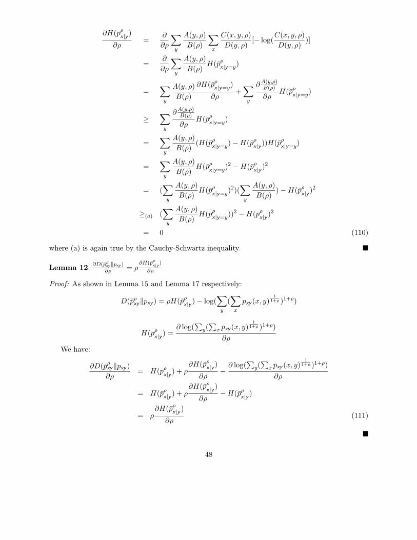
∂H(pρ

x |y )

∂ρ=

∂

∂ρ

∑

y

A(y, ρ)

B(ρ)

∑

x

C(x, y, ρ)

D(y, ρ)[− log(

C(x, y, ρ)

D(y, ρ))]

=∂

∂ρ

∑

y

A(y, ρ)

B(ρ)H(pρ

x |y=y)

=∑

y

A(y, ρ)

B(ρ)

∂H(pρ

x |y=y)

∂ρ+∑

y

∂ A(y,ρ)B(ρ)

∂ρH(pρ

x |y=y)

≥∑

y

∂ A(y,ρ)B(ρ)

∂ρH(pρ

x |y=y)

=∑

y

A(y, ρ)

B(ρ)(H(pρ

x |y=y) − H(pρ

x |y ))H(pρ

x |y=y)

=∑

y

A(y, ρ)

B(ρ)H(pρ

x |y=y)2 − H(pρ

x |y )2

= (∑

y

A(y, ρ)

B(ρ)H(pρ

x |y=y)2)(

∑

y

A(y, ρ)

B(ρ)) − H(pρ

x |y )2

≥(a) (∑

y

A(y, ρ)

B(ρ)H(pρ

x |y=y))2 − H(pρ

x |y )2

= 0 (110)

where (a) is again true by the Cauchy-Schwartz inequality. �

Lemma 12∂D(pρ

xy‖pxy )∂ρ

= ρ∂H(pρ

x|y)

∂ρ

Proof: As shown in Lemma 15 and Lemma 17 respectively:

D(pρxy‖pxy ) = ρH(pρ

x |y ) − log(∑

y

(∑

x

pxy (x, y)1

1+ρ )1+ρ)

H(pρ

x |y ) =∂ log(

∑

y(∑

x pxy (x, y)1

1+ρ )1+ρ)

∂ρ

We have:

∂D(pρxy‖pxy )

∂ρ= H(pρ

x |y ) + ρ∂H(pρ

x |y )

∂ρ−

∂ log(∑

y(∑

x pxy (x, y)1

1+ρ )1+ρ)

∂ρ

= H(pρ

x |y ) + ρ∂H(pρ

x |y )

∂ρ− H(pρ

x |y )

= ρ∂H(pρ

x |y )

∂ρ(111)

�

48

Lemma 13 sign∂[D(pρ

xy‖pxy )−H(pρ

x|y)]

∂ρ= sign(ρ − 1).

Proof: Using the previous lemma, we get:

∂D(pρxy‖pxy ) − H(pρ

x |y )

∂ρ= (ρ − 1)

∂H(pρ

x |y )

∂ρ

Then by Lemma 11, we get the conclusion. �

Lemma 14

ρH(pρxy

) − (1 + ρ) log(∑

y

∑

x

pxy (x, y)1

1+ρ ) = D(pρxy‖pxy )

Proof: By noticing that log(pxy (x, y)) = (1 + ρ)[log(pρxy (x, y)) + log(

∑

s,t pxy (s, t)1

1+ρ )]. We have:

D(pρxy‖pxy ) = −H(pρ

xy) −

∑

x,y

pρxy

(x, y) log(pxy (x, y))

= −H(pρxy

) −∑

x,y

pρxy

(x, y)(1 + ρ)[log(pρxy

(x, y)) + log(∑

s,t

pxy (s, t)1

1+ρ )]

= −H(pρxy

) + (1 + ρ)H(pρxy

) − (1 + ρ)∑

x,y

pρxy

(x, y) log(∑

s,t

pxy (s, t)1

1+ρ )

= ρH(pρxy

) − (1 + ρ) log(∑

s,t

pxy (s, t)1

1+ρ ) (112)

�

Lemma 15

ρH(pρ

x |y ) − log(∑

y

(∑

x

pxy (x, y)1

1+ρ )1+ρ) = D(pρxy‖pxy )

Proof:

D(pρxy‖pxy ) =

∑

y

∑

x

A(y, ρ)

B(ρ)

C(x, y, ρ)

D(y, ρ)log(

A(y,ρ)B(ρ)

C(x,y,ρ)D(y,ρ)

pxy (x, y))

=∑

y

∑

x

A(y, ρ)

B(ρ)

C(x, y, ρ)

D(y, ρ)[log(

A(y, ρ)

B(ρ)) + log(

C(x, y, ρ)

D(y, ρ)) − log(pxy (x, y))]

= − log(B(ρ)) − H(pρ

x |y ) +∑

y

∑

x

A(y, ρ)

B(ρ)

C(x, y, ρ)

D(y, ρ)[log(D(y, ρ)1+ρ) − log(C(x, y, ρ)1+ρ)]

= − log(B(ρ)) − H(pρ

x |y ) + (1 + ρ)H(pρ

x |y )

= − log(∑

y

(∑

x

pxy (x, y)1

1+ρ )1+ρ) + ρH(pρ

x |y )

�

49

Lemma 16

H(pρxy

) =∂(1 + ρ) log(

∑

y

∑

x pxy (x, y)1

1+ρ )

∂ρ

Proof:

∂(1 + ρ) log(∑

y

∑

x pxy (x, y)1

1+ρ )

∂ρ

= log(∑

t

∑

s

pxy (s, t)1

1+ρ ) −∑

y

∑

x

pxy (x, y)1

1+ρ

∑

t

∑

s pxy (s, t)1

1+ρ

log(pxy (x, y)1

1+ρ )

= −∑

y

∑

x

pxy (x, y)1

1+ρ

∑

t

∑

s pxy (s, t)1

1+ρ

log(pxy (x, y)

11+ρ

∑

t

∑

s pxy (s, t)1

1+ρ

)

= H(pρxy

) (113)

�

Lemma 17

H(pρ

x |y ) =∂ log(

∑

y(∑

x pxy (x, y)1

1+ρ )1+ρ)

∂ρ

Proof: Notice that B(ρ) =∑

y(∑

x pxy (x, y)1

1+ρ )1+ρ, and ∂B(ρ)∂ρ

= B(ρ)H(pρ

x |y ) as shown in Lemma 10.It is clear that:

∂ log(∑

y(∑

x pxy (x, y)1

1+ρ )1+ρ)

∂ρ=

∂ log(B(ρ))

∂ρ

=1

B(ρ)

∂B(ρ)

∂ρ

= H(pρ

x |y ) (114)

�

References

[1] Stephen Boyd and Lieven Vandenberghe. Convex Optimization. Cambridge University Press,2004.

[2] C. Chang and A. Sahai. The error exponent with delay for lossless source coding. IEEEInformation Theory Workshop, March 2006.

[3] C. Chang and A. Sahai. Upper bound on error exponents with delay for lossless source codingwith side-information. Proc. Int. Symp. Inform. Theory, July 2006.

50

[4] T. M. Cover. A proof of the data compression theorem of Slepian and Wolf for ergodic sources.IEEE Trans. Inform. Theory, 21:226–228, March 1975.

[5] I. Csiszar and J. Korner. Information Theory, Coding Theorems for Discrete MemorylessSystems. Akademiai Kiado, 1981.

[6] S. C. Draper. Universal incremental slepian-wolf coding. In Proc. 42nd Allerton Conf. onCommunication, Control and Computing, October 2004.

[7] S. C. Draper and A. Sahai. Noisy feedback improves communication reliability. In Proc. Int.Symp. Inform. Theory, 2006.

[8] G. Forney. Convolutional codes iii. sequential decoding. Information and Control, 25(3):267–297, 1974.

[9] R. G. Gallager. Source coding with side information and universal coding. Technical ReportLIDS-P-937, Mass. Instit. Tech., 1976.

[10] F. Jelinek. Buffer overflow in variable length coding of fixed rate sources. IEEE Trans. Inform.Theory, 14:490–501, May 1968.

[11] P. Koulgi, E. Tuncel, S. Regunathan, and K. Rose. On zero-error coding of correlated sources.IEEE Trans. Inform. Theory, 49:2856–2873, November 2003.

[12] A. Lapidoth and P. Narayan. Reliable communication under channel uncertainty. IEEE Trans.Inform. Theory, 44:2148–2177, October 1998.

[13] A. Sahai and T. Simsek. On the variable-delay reliability function of discrete memorylesschannels with access to noisy feedback. In IEEE Information Theory Workshop, San Antonio,Texas, 2004.

[14] Anant Sahai. Why block length and delay are not the same thing. Submitted to IEEE Trans.Inform. Theory, 2006.

[15] Anant Sahai and Sanjoy Mitter. Source coding and channel requirements for unstable pro-cesses. Submitted to IEEE Trans. Inform. Theory, 2006.

[16] D. Slepian and J. K. Wolf. Noiseless coding of correlated information sources. IEEE Trans.Inform. Theory, 19:471–480, July 1973.

[17] L. Weng, S. Pradhan, and A. Anastasopoulos. Error exponent regions for gaussian broadcastand mulitple access channels. submitted to Transactions on Information Theory, 2005.

51