LossCalcTM: Moody’s Model for Predicting Loss Given ... · This report describes and documents LossCalc, Moody's model for predicting loss given default ... bonds, and preferred

LossCalc

: Moody’s

Model fo

r Pre

dic

ting Lo

ss G

iven D

efa

ult (LG

D)

February 2002

Contact PhoneAndré Salaam 1.212.553.1653David Bren

AuthorsGreg M. GuptonRoger M. Stein

LossCalcTM: Moody’s Model forPredicting Loss Given Default (LGD)

Special Comment

continued on page 3

Specia

l Com

ment

This report describes and documents LossCalc, Moody's model for predicting loss given default(LGD): the equivalent of (1 - recovery rate). LGD is of natural interest to investors and lenderswishing to estimate future credit losses. LossCalc is a robust and validated model of UnitedStates LGD for bonds, loans, and preferred stock. It produces estimates of LGD for defaultsoccurring immediately and for defaults occurring in one year. These two point-in-time esti-mates can be used to predict LGD over holding periods.

LossCalc is a statistical model that incorporates information on instrument, firm, industry,and economy to predict LGD. It improves upon traditional reliance on historical recovery aver-ages. The model is based on over 1,800 observations of U.S. recovery values of defaulted loans,bonds, and preferred stock covering the last two decades. This dataset includes over 900defaulted public and private firms in all industries.

We believe LossCalc is a meaningful addition to the practice of credit risk management anda step forward in answering the call for rigor that the BIS has outlined in their recently proposedBasel Capital Accord.

Figure 1 Recovery Experience and Forecasts for Senior Unsecured Bonds over TimeThis figure shows the predicted average recoveries over time of LossCalc (thick red line) versus the long-term average as it evolvesover time (thin line). The bars show the actual recovery for each year. Dark colored bars indicate years with smaller sample size.

Senior Unsecured Bond Recoveries over Time

$20

$30

$40

$50

$60

$70

'85 '86 '87 '88 '89 '90 '91 '92 '93 '94 '95 '96 '97 '98 '99 '00 '01

Reco

very

Val

ue

Year's Actual Recoveries LossCalc Historical Average

2 Moody’s Rating Methodology

© Copyright 2002 by Moody’s Investors Service, Inc., 99 Church Street, New York, New York 10007. All rights reserved. ALL INFORMATION CONTAINED HEREIN ISCOPYRIGHTED IN THE NAME OF MOODY’S INVESTORS SERVICE, INC. (“MOODY’S”), AND NONE OF SUCH INFORMATION MAY BE COPIED OR OTHERWISEREPRODUCED, REPACKAGED, FURTHER TRANSMITTED, TRANSFERRED, DISSEMINATED, REDISTRIBUTED OR RESOLD, OR STORED FOR SUBSEQUENT USE FORANY SUCH PURPOSE, IN WHOLE OR IN PART, IN ANY FORM OR MANNER OR BY ANY MEANS WHATSOEVER, BY ANY PERSON WITHOUT MOODY’S PRIORWRITTEN CONSENT. All information contained herein is obtained by MOODY’S from sources believed by it to be accurate and reliable. Because of the possibility ofhuman or mechanical error as well as other factors, however, such information is provided “as is” without warranty of any kind and MOODY’S, in particular, makes norepresentation or warranty, express or implied, as to the accuracy, timeliness, completeness, merchantability or fitness for any particular purpose of any such information.Under no circumstances shall MOODY’S have any liability to any person or entity for (a) any loss or damage in whole or in part caused by, resulting from, or relating to,any error (negligent or otherwise) or other circumstance or contingency within or outside the control of MOODY’S or any of its directors, officers, employees or agents inconnection with the procurement, collection, compilation, analysis, interpretation, communication, publication or delivery of any such information, or (b) any direct,indirect, special, consequential, compensatory or incidental damages whatsoever (including without limitation, lost profits), even if MOODY’S is advised in advance of thepossibility of such damages, resulting from the use of or inability to use, any such information. The credit ratings, if any, constituting part of the information containedherein are, and must be construed solely as, statements of opinion and not statements of fact or recommendations to purchase, sell or hold any securities. NOWARRANTY, EXPRESS OR IMPLIED, AS TO THE ACCURACY, TIMELINESS, COMPLETENESS, MERCHANTABILITY OR FITNESS FOR ANY PARTICULAR PURPOSE OFANY SUCH RATING OR OTHER OPINION OR INFORMATION IS GIVEN OR MADE BY MOODY’S IN ANY FORM OR MANNER WHATSOEVER. Each rating or otheropinion must be weighed solely as one factor in any investment decision made by or on behalf of any user of the information contained herein, and each such user mustaccordingly make its own study and evaluation of each security and of each issuer and guarantor of, and each provider of credit support for, each security that it mayconsider purchasing, holding or selling. Pursuant to Section 17(b) of the Securities Act of 1933, MOODY’S hereby discloses that most issuers of debt securities (includingcorporate and municipal bonds, debentures, notes and commercial paper) and preferred stock rated by MOODY’S have, prior to assignment of any rating, agreed to pay toMOODY’S for appraisal and rating services rendered by it fees ranging from $1,000 to $1,500,000. PRINTED IN U.S.A.

Authors

Greg M. GuptonRoger M. Stein

Production Associate

Marisela Guzmán

Moody’s Rating Methodology 3

We have organized the remainder of this report as follows:

Section 1, Loss Given Default: discusses the importance and difficulty of estimating loss given default(LGD), which is of natural interest to investors and lenders. Its estimation is as important as the prob-ability of default in predicating credit losses.

Section 2, The LossCalc Model: describes the LossCalc LGD model and summarizes the factors ofthe model, the modeling framework, model validation results, and the dataset. We discuss each ofthese topics in more detail in subsequent sections.

Section 3, Factors: describes the nine predictive factors that drive the estimate of LGD in theLossCalc model.

Section 4, Framework: describes the modeling approach we used to develop LossCalc.

Section 5, Validation and Testing: documents the performance of the model in out-of-sample, out-of-time testing, which we find to be superior to traditional LGD estimation methods.

Section 6, The Dataset: describes the data used to develop the model and gives details of the datasetwhich contains over 1,800 observations of U.S. recovery values of defaulted loans, bonds, and pre-ferred stock covering the last two decades.

Highlights

1. We describe Moody's LossCalc™, a predictive statistical model of loss given default (LGD), the fac-tors in the model, the modeling approach, and the accuracy of the model.

2. We find that LossCalc performs better at predicting LGD than traditional historical average methods.LossCalc:

• exhibits lower prediction error and higher correlation with actual losses;• is more powerful at predicting low recoveries; and• produces narrower confidence bounds.

3. LossCalc produces estimates of LGD for defaults occurring immediately and for defaults occurringin one year.

4. Moody's has based LossCalc on over 1,800 observations of U.S. recovery values of defaulted loans,bonds, and preferred stock covering the last two decades. This dataset includes over 900 defaultedpublic and private firms in all industries.

AcknowledgementsThe authors would like to thank the numerous individuals who contributed to the ideas, modeling, valida-tion, testing and ultimately writing of this document. Eduardo Ibarra provided significant research sup-port for this project. We also thank the following people for their comments: Richard Cantor, Lea V.Carty, Jerome Fons, Daniel Gates, and Douglas Lucas, all of Moody's; Dr. Philipp J. Schönbucher, ofBonn University; and Prof. Jeffrey S. Simonoff, of New York University; and Phil Escott, of Oliver,Wyman & Company.

We also received invaluable feedback from Moody's Academic Advisory and Research Committeeduring the presentation of this model and in discussions afterwards, particularly Darrell Duffie, ofStanford University; William Perraudin, of Birkbeck College; and John Hull, of the University ofToronto. Moody's Quantitative Tools Standing Committee also provided helpful suggestions that greatlyimproved the model.


Table of ContentsACKNOWLEDGEMENTS .................................................................................................................. 4

TABLE OF CONTENTS ...................................................................................................................... 5

1. LOSS GIVEN DEFAULT .............................................................................................................. 6

2. THE LOSSCALC LGD MODEL ................................................................................................ 72.1 OVERVIEW............................................................................................................................................................ 72.2 TIME HORIZON .................................................................................................................................................. 72.3 FACTORS .............................................................................................................................................................. 82.4 FRAMEWORK ...................................................................................................................................................... 82.5 VALIDATION........................................................................................................................................................ 82.6 THE DATASET .................................................................................................................................................... 9

3. FACTORS ........................................................................................................................................ 93.1 DEFINITION OF LOSS GIVEN DEFAULT .............................................................. 93.2 FACTOR DESCRIPTIONS ............................................................................................ 10

3.2.1 Debt Type and Seniority ........................................................................................ 11a 3.2.2 Firm Specific Capital Structure: Leverage ............................................................ 12

3.2.3 Industry.................................................................................................................... 123.2.4 Macro Economic .................................................................................................... 13

4. FRAMEWORK ................................................................................................................................ 144.1 ESTABLISHING A DEPENDENT VARIABLE .......................................................... 144.2 TRANSFORMATION AND MINI-MODELING ...................................................... 16

4.2.1 The Index of Macro Changes ................................................................................ 164.2.2 Factor Inclusion by Seniority Class and Sector .................................................... 16

4.3 MODELING AND MAPPING:EXPLANATION TO PREDICTION .................... 164.4 CONFIDENCE INTERVAL ESTIMATION .............................................................. 16

5. VALIDATION AND TESTING .................................................................................................. 175.1 ALTERNATIVE RECOVERY MODELS USED AS BENCHMARKS .................... 17

5.1.1 Table of Historical Averages .................................................................................. 175.1.2 The Historical Mean Recovery Rate...................................................................... 18

5.2 THE LOSSCALC VALIDATION TESTS .................................................................... 185.2.1 Prediction error rates .............................................................................................. 185.2.2 Correlation with actual recoveries.......................................................................... 205.2.3 Relative performance for specific debt types.......................................................... 215.2.4 Prediction of larger than expected losses .............................................................. 225.2.5 Reliability and Width of Confidence Intervals ...................................................... 23

6. THE DATASET .............................................................................................................................. 256.1 HISTORICAL TIME PERIOD ANALYZED................................................................ 256.2 SCOPE OF GEOGRAPHIC COVERAGE AND LEGAL DOMAIN ........................ 266.3 SCOPE OF FIRM TYPES AND INSTRUMENT CATEGORIES ............................ 26

7. CONCLUSION .............................................................................................................................. 27APPENDIX A: BETA TRANSFORMATION TO NORMALIZE LOSS DATA ...................... 28APPENDIX B: AN OVERVIEW OF THE VALIDATION APPROACH .................................. 29

B.1.CONTROLLING FOR "OVER FITTING" RISK: WALK-FORWARD TESTING 29B.2.RESAMPLING .................................................................................................................... 30

GLOSSARY OF TERMS ........................................................................................................................ 31BIBLIOGRAPHY...................................................................................................................................... 32


1. Loss Given DefaultLoss Given Default, the equivalent of (1 - recovery rate) is of natural interest to investors and lenders whowish to estimate potential credit losses. However, it is inherently difficult to predict what the value or cashflows of an obligation might be if it became defaulted. When a loan is made or a security purchased, theholder does not normally think it likely that the obligor will default. Yet, to predict LGD, the creditormust imagine the circumstances that would cause default and the condition of the obligor after such default.

The practicalities of the U.S. bankruptcy process make it difficult to predict how the value of a bank-rupt firm will be apportioned among its creditors. In U.S. bankruptcy legislation, the guiding principalfor allocating a firm's liquidation value amongst its creditors is the seniority hierarchy or "classes" ofclaims applied using the Absolute Priority Rule. In its strictest interpretation, each class has a relative rank-ing. Funds available for distributions are paid first to the highest-ranking class until the firm's obligationsto it are fully satisfied. Only then would the next highest-ranking class start to be paid.

This strict interpretation of priority is almost never fully adhered to (see for example Longhofer &Carlstrom [1995]). Indeed, bankruptcy procedures include the drafting of a "plan" that can only proceedspeedily upon the approval of multiple levels of claimants. Thus, to gain control of the company quickly,and stop any further deterioration of asset values from occurring, there is incentive for senior claimants tomake concessions to junior claimants. In the end, recovery rates have a lot to do with not only the assetsof the bankrupt firm and the seniority of a petitioner's claim, but also the relative strength of negotiatingpositions.

LGD is as important as the probability of default in estimating potential credit losses. We can see thisimmediately by considering the formula for credit loss:

Potential Credit Loss = Probability of Default x Loss Given Default

A proportional error in either the probability of default or LGD affects potential credit losses identically.Yet, much more resource and effort is employed to estimate probability of default. Many different model-ing techniques are applied to default probability; from statistical methods based on accounting data tostructural (Merton) models to hybrids such as Moody's RiskCalc™.

In sharp contrast, LGD is typically estimated by appealing to historical averages, usually segregated bydebt type (loans, bonds and preferred stock) and seniority (secured, senior unsecured, subordinate, etc.).Figure 2 displays detailed historical information on recoveries.

Figure 2 Default Recovery by Debt Type and Seniority, 1981-2000This figure is adapted from Moody's 2001 annual default study; see Exhibit #20 in Hamilton, Gupton & Berthault [2001]. It highlights the widevariability of recoveries even within individual seniority classes. The shaded boxes cover the inter-quartile range with the median marked as awhite horizontal line. Squared brackets cover the data range except for outliers that are marked as horizontal lines.


Secured Unsecured Senior Senior Senior Subordinated Junior Preferred Secured Unsecured Subordinated Subordinated

Bank Loans Bonds Stocks

110

90

70

50

30

10

Pric

e/Pe

rform

ance

Per

US$

100

Par

The extreme range of the historical data should make one wonder about its use. For example, supposeone used the median (32%) to estimate recovery on a senior subordinated bond. The median absoluteerror of that estimate (out of sample) is over 22%. Compared to the 32% median, the range of the erroris almost 70% (=22/32) of the estimate. The same percentage absolute error in default probabilities for asenior subordinated bond with a senior implied rating of Baa and a 10-year maturity would imply a histor-ical default rate somewhere in the very wide range of Aa-to-almost-Ba!1

Recently, regulatory bodies have focused more closely on LGD analysis. The proposed New BaselCapital Accord (Basel, 2001) addresses the issue explicitly:

Where there is no explicit maturity dimension in the foundation approach, corporate exposures will receive a risk weight that depends on the probability of default (PD)

and loss given default (LGD). (Basel, § 173)

Banks would have the option of using conservative pre-defined LGD measures under the so-calledfoundation approach, but if they wish to qualify for the advanced approach:

…A bank must estimate an LGD for each of its internal LGD grades…Each estimate of LGD must be grounded in historical experience and empirical evidence. At the same time, these estimates must be forward looking…LGD estimates that are based purely on subjective or

judgmental consideration and not grounded in historical experience and data will be rejected by supervisors. (Basel, § 336 & 337)

We believe that LossCalc is a meaningful addition to the practice of credit risk management and a step for-ward in answering the call for rigor that the BIS has outlined in their recently proposed Basel Capital Accord.

2. The LossCalc LGD Model

2.1 OVERVIEWLossCalc is a robust and validated model of United States LGD for bonds, loans, and preferred stock. Itproduces estimates of LGD for defaults occurring immediately and for defaults occurring in one year.

The issue of prediction horizon has received little attention in previous recovery research, perhaps due tothe static nature of a typical table of long-term historical averages. Applications of historical average tablestypically use the same estimate of recovery irrespective of the horizon over which default might occur. Thismeans that important considerations are ignored such as the point in the credit cycle or the sensitivity of aborrower to the economic environment. It is the nature of historical average LGD methods to be updatedinfrequently. In addition, new data will have a relatively small impact on longer-term averages.

In contrast, LossCalc is dynamic and able to give a more exact specification of LGD horizon that incor-porates cyclic and firm specific effects. LossCalc's immediate and one-year horizon forecasts would natu-rally fit different investor and risk management applications.

LossCalc incorporates information on instrument, firm, industry, and economy to predict LGD. Itimproves upon traditional reliance on historical recovery averages. We have developed the model on over1,800 observations of U.S. recovery values of defaulted loans, bonds, and preferred stock covering the lasttwo decades. This dataset includes over 900 defaulted public and private firms in all industries.

2.2 TIME HORIZONThe time horizon of LGD projections is an important aspect of credit risk that has unfortunately beenabsent from risk management practices. The valuation of a defaulted debt is far from static and shouldchange with different forecast horizons. This is true for the valuation of any asset. Investors and lendersshould match the tenor of the LGD projection to their exposure horizon.

1 The 10-year default rate on a Baa is just under 8% (here we round from the historical 7.92% rate). Using the mean absolutedeviation as a measure of error, we observed about a 22/32 » 70% error rate on the LGD estimate. The equivalent 70% difference indefault probability would imply:

a lower bound of: 8% - 0.7*8% = 2.4%; andan upper bound of: 8% + 0.7*8% =13.6%.

The Aa 10-year default rate is 3.1%, which is still higher than our lower bound, so the upper bound would be equivalent to at least aAa-rating. The upper bound is below the 10-year Baa default rate of 7.92% and above the 10-year Ba default rate of 19.05%. Referto Exhibits #30 and #31 in Keenan, Hamilton & Berthault [2000] for the default rates. This is a stylized example.


Nevertheless, the prevailing practice is to treat LGD as static over the holding period. LossCalc pro-jects LGD for two points in time: immediate and at one year. Assuming no knowledge of the individualobligor, the average time of a possible default would be about half way into the exposure period. Thismeans that LossCalc's immediate prediction of LGD should be applied to exposures maturing in less thanone year and with an average time to default of less than six-months. The immediate version can also beused for debts that are already in default, particularly if market prices are not available.

The one-year version of LossCalc projects LGD for default in one year. Therefore, it is ideal for two-year exposures that have an average time to default of one year. The one-year LossCalc LGD is also thebest prediction for exposures one year and greater. The user should note changes in exposure amountwhen determining which LGD projection to use.

2.3 FACTORSAs a proxy for the ultimate recovery on a defaulted instrument, we use the market value of defaulted debtone-month after default.

LossCalc uses nine explanatory factors to predict LGD. We have summarized these nine factors intofour broad groups as shown below:

• debt-type (i.e., loan, bond, and preferred stock) and seniority grade (e.g., secured, senior unse-cured, subordinate, etc.);

• firm specific capital structure: leverage and seniority standing;• industry: moving average of industry recoveries; banking industry indicator;• macroeconomic: one-year median RiscCalc default probability; Moody's Bankrupt Bond Index;

trailing 12-month speculative grade default rate; changes in the index of Leading EconomicIndicators.

These factors have little intercorrelation, each is statistically significant, and together they make amore accurate prediction of LGD.

2.4 FRAMEWORKWe have based LossCalc on a methodological framework similar to that used in Moody's RiskCalc proba-bility of default models. The broad steps in this framework are transformation, modeling, and mapping.

Transformation: We transform raw data into "mini-models." For example, we have found it useful totransform certain macro-economic variables into composite indices, rather than use the pure levels. Asanother example, we find it useful to use average historical LGD by debt type and seniority.

Modeling: Once we have transformed individual factors and converted them into mini-models, weaggregate these using regression techniques.

Mapping: We statistically map the model output to historical LGD.

Each of the three steps to this process relies on the application of standard statistical techniques. Weoutline the details of these in Section 4.

2.5 VALIDATIONWe find that LossCalc is a better predictor of LGD than the traditional methodologies of historical aver-ages segmented by debt type and seniority. By "better," we mean that:

• LossCalc estimates have significantly lower error.• LossCalc makes far fewer large errors. A reduction in very large errors is the principal driver of the

overall reduction in error. For example, LossCalc has about 50% fewer errors larger than 30% ofpar value.

• LossCalc estimates have significantly more correlation with actual outcomes. This means they havebetter tracking of high and low recoveries.


• LossCalc provides better discrimination between instruments of the same type. For example, the model pro-vides a much better ordering (best to worst recoveries) of bank loans than historical averages.

• Over 10% of the time, the reduction in error rate is greater than 12% of original par value.• LossCalc, on average, has tighter confidence bounds than other approaches so there is more certainty of

recovery prediction.

2.6 THE DATASETWe developed the model on over 1,800 observations of U.S. LGD of defaulted loans, bonds, and pre-ferred stock covering the last two decades. This dataset includes over 900 defaulted public and privatefirms in all industries. The issue sizes range from $680 thousand to $2.0 billion, with a median size ofabout $100 million. The median firm size (assets at annual report before default) was $660 million, butranged from $5.0 million to $37.7 billion. Neither debt size nor firm size appears significantly predictiveof recovery rate in this dataset.

3. FactorsIn this section, we describe the LGD variable and the explanatory factors of the immediate and one-yearLossCalc models. The modeling framework is a statistical modeling approach. The central goal is toincrease predictive power through the inclusion of multiple factors, each designed to capture specificaspects of LGD determination.

3.1 DEFINITION OF LOSS GIVEN DEFAULTWe define recovery on a defaulted instrument as its market value approximately one-month after default.2Importantly, we use security-specific bid-side market quotes.3 These prices are not "matrix" prices, whichare broker-created tables specified across maturity, credit grade, and instrument type, without considera-tion of the specific issuer.

Moody's chose to use price observations one month after default for three reasons:

• it gives the market sufficient time to assimilate new post-default corporate information;• it is not so long after default that market quotes become too thin for reliance;• the period best aligns with the goal of many investors to trade out of newly defaulted debt.

This definition of recovery value avoids the practical difficulties associated with determining the post-default cash flows of a defaulted debt or the value of instruments provided in replacement of the defaulteddebt. The very long resolution times in a typical bankruptcy proceeding compounds these problems.

Figure 3 shows the timing of price observation of recovery estimates and the ultimate resolution of theclaims. Broker quotes on defaulted debt provide a far more timely recovery valuation relative to waitingto observe the completion of court ordered resolution payments. Market quotes are commonly availablein the period 15-to-60 days after default. However, if no pricing was available or if we felt that a price wasnot reliably stated, then it did not enter our dataset.

2 This date is not always well defined. As an example, bank loan covenants are commonly written with terms that are more sensitive tocredit distress than those of bond debentures. Thus, different debt obligations of a single defaulted firm may officially default ondifferent dates. The vast majority of securities in our dataset are quoted within the range of 15-to-60 days of the date assigned to initialdefault of the firm's public debt. Our study found no distinction in the quality or explicability of default prices across this 45-day range.

3 Contributed by Goldman Sachs, Citibank, BDS Securities, Loan Pricing Corporation, Merrill Lynch, and Lehman Brothers.


Figure 3 Timeline of Default Recovery EstimationThis diagram illustrates the timing of the observation of recovery estimates, as represented by the prices of defaulted securities and the ultimateresolution of the claims. Broker quotes on defaulted debt provide a far more timely recovery valuation relative to waiting to observe the comple-tion of court ordered resolution payments. Market quotes are commonly available 15-to-60 days post-default. Final resolution takes 1¾ years atleast half the time.

Although it is beyond the scope of this report, there have been several studies of the market's ability toprice defaulted debt efficiently.4 These studies do not always show statistically significant results, but theyconsistently support the market's efficient pricing of ultimate recoveries. At different times, Moody's hasstudied recovery estimates derived from both bid-side market quotes and discounted estimates of resolu-tion value. Both methods have their advantages and disadvantages. We find, consistent with outside aca-demic research, that these two tend to be unbiased estimates of each other.

3.2 FACTOR DESCRIPTIONSOver the course of model development, we considered the inclusion of a number of predictive variables.We included factors only if they have both a strong economic rationale and statistical significance.5

In all, the LossCalc models use nine factors to predict immediate LGD and a subset of eight factors topredict one-year LGD. We grouped the factors into four categories as shown in Table 1 below. Thetable highlights the four broad categories of predictive information: debt type and seniority, firm specificcapital structure, industry, and macro economic. These factors have little intercorrelation and togethermake a significant and more accurate prediction of LGD. All factors enter both LossCalc forecast hori-zons (i.e., immediate and one-year) with the single exception of the U.S. speculative-grade default rate.We chose to have this indicator enter only the immediate model.

4 See Eberhart & Sweeney [1992], Wagner [1996] and Ward & Griepentrog [1993].

5 Note that we also considered factors that were not included in the model due to either lower power than competing alternatives ordata sufficiency issues. They are not discussed here in detail. Some of these were: yields and spreads (e.g., BBB - AAA, Govt1,2...10y, etc.), other macro factors (e.g., CPI, etc.), other financial ratios (e.g., EBIT / Sales, Current Liabilities / Current Assets, etc.),other instrument specific information (e.g., coupon, spread, etc.), and so forth.


"Technical" Defaults

Company Default + 15

Days+ 60 Days

Market Pricing (BidSide Quotes)

Final Resolution1¾ Years Median

Accounting of Resolution(Often with unknown values)

Table 1 Explanatory Factors in the LossCalc ModelsThis is a summary of the factors applied in Moody's LossCalc model to predict LGD. The table highlights the four broad categories of predictiveinformation: instrument, firm, industry, and broad economic environment. These factors have little intercorrelation and together make a signifi-cant and more accurate prediction of LGD.

Although we do not publicly disclose the exact coefficients (weights) of our models, all of the factors inthe model are individually highly statistically significant and in all cases the signs were in the expecteddirection. Figure 4 below shows the contributions of each broad factor category to the prediction of one-year LGD.

Figure 4 Relative Influence of Different Factor Groups in Predicting LGDThis figure shows the normalized marginal effects (relative influence) of each broad factor when we hold all other factors at their average values.

3.2.1 Debt Type and SeniorityHistorical average recovery rates, broken-out by debt type (loan, bond, preferred stock) and seniority(secured, senior unsecured, subordinate, etc.) are the starting points for LossCalc. Although historicalaverages are important, they account for less than half of the influence in predicting levels of recoveries inLossCalc, as shown in Figure 4.


Debt Type and SeniorityHistorical average LGD by debt-type (loan, bond, and preferred stock) Historical Averagesand seniority (secured, senior unsecured, subordinate, etc.).

Firm-Specific Capital StructureSeniority standing of debt in the firm's overall capital structure; this is the Seniority Standingrelative seniority of a claim. Note that this is different from the absoluteseniority stated in Debt Type and Seniority above. The most senior obligation of a firm might be, for example, a subordinate note.

Firm leverage (Total Assets / Total Liabilities) Leverage

IndustryMoving average of normalized industry recoveries. We have here controlled Industry Experiencefor seniority class.

Banking industry indicator Banking Indicator

Macro EconomicOne-year median RiskCalc default probability across time. RiskCalcMoody's Bankrupt Bond Index, an index of prices of bankrupt bonds MBBITrailing 12-month speculative grade average default rate Speculative-Grade Default RateChanges in index of Leading Economic Indicators LEAD

Relative Influence of Factors

0% 10% 20% 30% 40%

Firm SpecificCapital Structure

Industry

Macro EconomicEnvironment

Debt Type

& Seniority

Inclusion of historical averages does two things. First, it addresses the effects of the Absolute PriorityRule of default resolution. Second, it helps ensure that, on average, LossCalc will perform no worse thanthe prevailing practice of referring to long-term historical averages.

The relative seniority of debt (i.e., the debt's rank within the capital structure of the firm) can beimportant to predicting LGD. For example, preferred stock is the lowest seniority class in a typical capitalstructure, but it might hold the highest seniority rank within a particular firm that has no funding fromloans or bonds in its capital structure. In addition, in cases where a firm issues debt sequentially in orderof seniority, it may happen that senior debt matures earlier leaving junior debt outstanding.

We designed LossCalc to consider a debt's seniority in absolute terms, via historical averages, and inrelative terms, when such data are available, within a particular firm. Both are predictive of LGD and arereasonably uncorrelated with one another. The relationship is well documented and straightforward.Each seniority class must compete with other classes for available funds.

It is reasonable to ask why we did not use a predictor such as "the dollar amount of debt that standsmore senior" or "the proportion of total liabilities that is more senior?" While these seem intuitivelymore appealing, there are two main reasons we chose the simpler indicator:

Resolution Procedure: In bankruptcy proceedings, a junior claimant's ability to extract concessions frommore senior claimants is not directly proportional to his claim size. Junior claimants can force the full dueprocess of a court hearing and so have a practical veto power on the speediness of an agreed settlement.6

Availability of Data: Claim amounts at the time of default are not the same as original issuance/borrow-ing amounts. In many cases, obligations are paid down in part before the full maturity of the debt.Sinking funds (for bonds) and amortization schedules (for loans) are examples of this. Determiningthe exposure at default for many obligations can be challenging, particularly for firms that pursue mul-tiple funding channels. In many cases, this data is unavailable. Requiring such an extensive detailingof claims before being able to make any LGD forecast would be onerous from both a modeling andusage perspective.

3.2.2 Firm Specific Capital Structure: LeverageIntuitively, the capital structure of a firm is relevant to the funds available (in default) for the satisfactionof creditor claims. Said another way, the assets to liabilities ratio acts like a coverage ratio of the fundsavailable versus the claims to be paid. A higher ratio of assets to liabilities is better.

However, leverage does not contribute to the prediction of LGD for secured credits. Such claimswould look first to the value of their specific security and only secondarily seek satisfaction from the gen-eral funds of the defaulted firm.

3.2.3 IndustryResearchers frequently propose industry level segregation of recovery levels as being useful in recoverymodeling.7 The idea is that an industry might consistently enjoy high recoveries or perhaps suffer recov-eries that are consistently low across time. Our test of this was to compile average industry recovery levelsacross time and test the statistical significance in the average's deviation from the overall average recovery.

We found this to work well for recoveries of bank defaults, which are consistently low across time. Therationale for modeling the banking industry by an indicator variable is as follows:

Seniority of Deposits over Public Debt: Deposits are commonly the majority of obligations of a bank andthey enjoy a "super-seniority" position relative to public debt in bankruptcy.

Liquidity of Banks: Unlike the plant and equipment found in other industries, the financial assets andliabilities of a bank are typically very short in duration and liquid. In response to this short-termnature (and to help stem systemic liquidity crisis), the Federal Reserve offers access to liquidity via theFed's Discount Window. Thus, it is difficult for creditors to "force" liquidity default on a bank thatstill has many good quality assets available to pay off its liabilities. Consequently, by the time banksdefault it is sometimes too late, when most of the good assets are insufficient.

6 We tested this on a sub-population selected to have fully populated claim amount records. The best predictor of recoveries, bothunivariately and in combination with a core set of LossCalc regressors was a simple flag of standing the highest. As alternatives, wetested dollars (and log of dollars) of superior claims and proportion of superior claims.

7 See Altman & Kishmore [1996] and Ivorski [1997] for broad recovery findings by industry and Borenstein & Rose [1995] for a singleindustry (airlines) case study.


Fed Forbearance: Historically, bank regulators have allowed insolvent banks to remain open. Duringthe time that regulators allow insolvent banks to remain open, banks use up their assets to pay offshort-term liabilities and the available asset coverage for long-term creditors falls proportionately.

However, we also found strong evidence of industry specific ebbs and flows in the recovery rates thatdiffered in time between industries. We found that some industries would enjoy periods of prolongedsuperior recoveries, but fall well below average recoveries at other times. A simple industry bump-up ornotch-down, held constant over time, does not capture this behavior. To address this, we grouped firmsinto twelve broad industries and created moving averages of recoveries.8

3.2.4 Macro EconomicThe intuition behind the inclusion of macro economic variables is that defaulted debt prices tend to riseand fall together as a population rather than being fully independent of one other. Another way of sayingthis is that recoveries have positive and significant intercorrelation within bands of time. This type of cor-relation has potentially material implications for portfolio calculations of Credit Value-at-Risk. The lead-ing vendor models of Cr-VaR implicitly set this correlation to zero and would thus understate Cr-VaR inthis regard.

3.2.4.1 One-Year RiskCalc Probability of DefaultMoody's RiskCalc for Public companies can measure changes in the credit quality of corporate obligorswith publicly traded equity. RiskCalc is a hybrid model that combines two credit risk modeling approach-es: (a) a structural model based on Merton's options-theoretic view of firms; and (b) a statistical modeldetermined through empirical analysis of historical accounting data. LossCalc uses time series of medianRiskCalc PDs.

3.2.4.2 Moody's Bankrupt Bond IndexLossCalc uses Moody's Bankrupt Bond Index (MBBI), a monthly price index measuring the return of abroad cross-section of long-term public debt issues of corporations that are currently in bankruptcy. Thebonds of defaulted or distressed companies that have not yet filed for bankruptcy are not included in theindex. MBBI includes both Moody's-rated and non-rated debt from U.S. and non-U.S. obligors, denomi-nated in U.S. dollars.9

3.2.4.3 Trailing 12-month Speculative Grade Average Default RatesWhile RiskCalc provides a measure of the outlook for default rates, we also found it useful to include ameasure of historical default rate behavior. We capture this through the inclusion of the trailing 12-month speculative grade default rate for Moody's rated firms. This factor did not exhibit strong predic-tive power for the one-year model and is thus included only in the immediate model where it was stronglysignificant.

3.2.4.4 Changes in Index of Leading Economic IndicatorsWe found that the change in Gross Domestic Product computed over the upcoming duration of default res-olution was strongly predictive of recoveries. Of course, this future information could never be availablefor prediction. Nonetheless, this relationship indicates something of the process underlying recoveries.

As a proxy, we chose a readily accessible series that seeks to address this same information, the Index ofLeading Economic Indicators.10 While its correlation with recoveries, as shown in Figure 5, is far fromperfect, it is reasonable and carries significant predictive power. There is visible correlation between itand a time-series of aggregated recovery experience.

8 Industry categories: Banking, Consumer Products, Energy, Financial (Non-Bank), Hotel/Gaming/Leisure, Industrial, Media,Miscellaneous, Retail, Technology, Transportation and Utilities.

9 The MBBI historical series was revised in January 2000. Refer to "The Investment Performance of Bankrupt Corporate DebtObligations", February 2000, Moody's Special Comment for details on this revision and about the construction of the MBBI.

10 The Conference Board, Inc. produces the Leading Economic Indicators. See their site at http://www.globalindicators.org, for details.


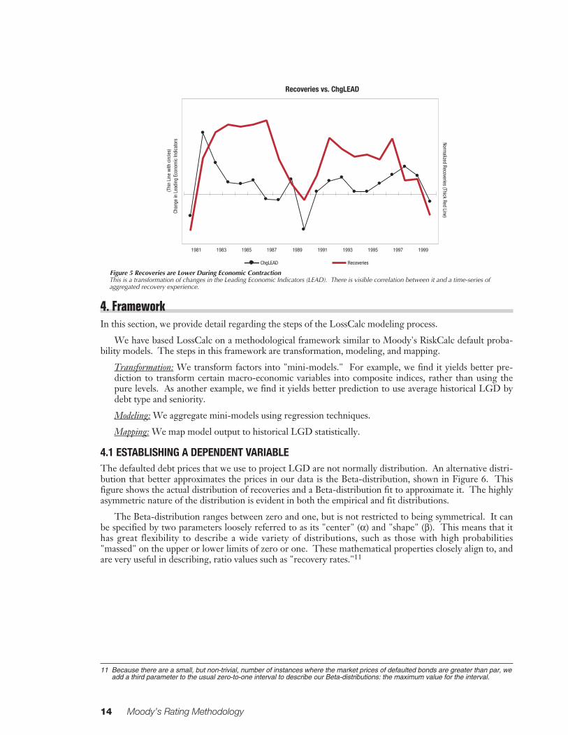
Figure 5 Recoveries are Lower During Economic ContractionThis is a transformation of changes in the Leading Economic Indicators (LEAD). There is visible correlation between it and a time-series ofaggregated recovery experience.

4. FrameworkIn this section, we provide detail regarding the steps of the LossCalc modeling process.

We have based LossCalc on a methodological framework similar to Moody's RiskCalc default proba-bility models. The steps in this framework are transformation, modeling, and mapping.

Transformation: We transform factors into "mini-models." For example, we find it yields better pre-diction to transform certain macro-economic variables into composite indices, rather than using thepure levels. As another example, we find it yields better prediction to use average historical LGD bydebt type and seniority.

Modeling: We aggregate mini-models using regression techniques.

Mapping: We map model output to historical LGD statistically.

4.1 ESTABLISHING A DEPENDENT VARIABLEThe defaulted debt prices that we use to project LGD are not normally distribution. An alternative distri-bution that better approximates the prices in our data is the Beta-distribution, shown in Figure 6. Thisfigure shows the actual distribution of recoveries and a Beta-distribution fit to approximate it. The highlyasymmetric nature of the distribution is evident in both the empirical and fit distributions.

The Beta-distribution ranges between zero and one, but is not restricted to being symmetrical. It canbe specified by two parameters loosely referred to as its "center" (α) and "shape" (β). This means that ithas great flexibility to describe a wide variety of distributions, such as those with high probabilities"massed" on the upper or lower limits of zero or one. These mathematical properties closely align to, andare very useful in describing, ratio values such as "recovery rates."11

11 Because there are a small, but non-trivial, number of instances where the market prices of defaulted bonds are greater than par, weadd a third parameter to the usual zero-to-one interval to describe our Beta-distributions: the maximum value for the interval.


Recoveries vs. ChgLEAD

1981 1983 1985 1987 1989 1991 1993 1995 1997 1999

Chan

ge in

Lea

ding

Eco

nom

ic In

dica

tors

(Thi

n Li

ne w

ith c

ircle

s)

Normalized Recoveries (Thick Red Line)

ChgLEAD Recoveries

Figure 6 Beta-distribution Fit to RecoveriesThis figure shows the actual distribution of recoveries and a Beta-distribution fit to approximate it. The highly asymmetric nature of the distribu-tion is evident in both the empirical and fit distributions.

In our dataset, the distribution of bond recoveries shows a characteristic left-side peak and right-sideskew. Figure 7, below, compares a Beta-distribution with the corresponding Gaussian (Normal) for thesame mean and SD. It is often more convenient to work with symmetrical distributions, such as theNormal, than with bounded and skewed ones, such as the Beta. Fortunately, the mathematical transfor-mation between the two is straightforward.

Figure 7 Recoveries are not Normally Distributed: Beta vs. Gaussian DistributionsThese probability density functions underscore the dramatic difference in shape between a Beta-distribution and the Normal distribution. TheBeta-distribution is bounded on both sides and this means that a probability "mass" can accumulate on one of its edges (see the peak above). Inaddition, it has no requirement that it be symmetrical about its mean. We selected this particular Beta curve to illustrate these behaviors.

We first group obligations according to debt-type (i.e., loans, bonds, and preferred stock) since thesebroad categories exhibit markedly different average recovery distributions. We then transform the vari-ables from Beta to Normal space. Conveniently, this only requires a) the mean, µ, and the standard devia-tion, σ, of the observed recoveries12 and b) the bounding values. Appendix A gives details of this parame-terization and transformation. The result is a normally distributed variable with the same probability asthe equivalent raw recovery had in Beta-space.

12 We expect that the particular values that we find for each debt-type's m and s (and so the parameter values that we assign to the a'sand b's) will change from time to time as we update LossCalc with additional data.


Market Bid Pricing 1-month post default

Rel

ativ

e Fr

eque

ncy

Observed Frequency

Beta-distribution Fit

-0.5 -0.4 -0.3 -0.2 -0.1 0.0 0.1 0.2 0.3 0.4 0.5 0.6 0.7 0.8 0.9 1.0

Normal Density Function Beta Density Function

St. Dev.=0.25%For both curves

Average = 40.1%For both curves

4.2 TRANSFORMATION AND MINI-MODELINGWe gained a great deal of insight by assessing predictive factors on a stand-alone (univariate) basis. Wetransform some of the input factors to make them better stand-alone predictors before assembling an"overall" model. If these transformations create a truly significant factor, then we typically rename itstransformation a "mini-model."

In LossCalc for example, both the Seniority-Class variable and the Industry LGD variable are "mini-models." Each is indicative on a stand-alone basis as a measure of recovery values. Other instances ofmini-modeling were less dramatic, such as a leverage ratio, logs, or changes versus levels in a time-series,etc. Two other model components are useful to note.

4.2.1 The Index of Macro ChangesLossCalc uses an index calculated by statistically weighting the changes in levels of various macro economicindicators into a composite index, which is in effect an estimate of the average recovery that would beimplied by these macro changes only.13 We do this weighing as we step forward in time each month. Thisboth maximizes its overall predictive power and minimizes month-to-month changes in the weighting.

4.2.2 Factor Inclusion by Seniority Class and IndustryThe model drops certain factors in certain cases. For example, although leverage is one of the nine predic-tive factors in the LossCalc model, it is not included in the case of financial institutions. These are typi-cally highly leveraged with lending and investment portfolios having very different implications than anindustrial firm's plant and equipment.

Similarly, we do not consider leverage when assessing secured debt. The recovery value of a secured obliga-tion depends primarily on the value of its collateral rather than the netted value of general corporate assets.

4.3 MODELING AND MAPPING: EXPLANATION TO PREDICTIONThe modeling phase of the LossCalc methodology involves statistically determining the appropriateweights to use in combining the transformed variables and mini-models described in the previous section.The combination of all the above predictive factors is a linear weighted sum, derived using regressiontechniques. The model takes the additive form:

Where the xi are the transformed values and mini-models described above, the βi, are the weights and is the normalized recovery. Note that at this point is stated in "normalized space" and still needs to

be transformed back into "dollar space." So the final step is to apply the inverse of the Beta-distributiontransformation (discussed above) to the three cases of loans, bonds, and preferred stock. See Appendix Afor more details.

4.4 CONFIDENCE INTERVAL ESTIMATIONLossCalc also provides an estimate of the confidence interval (i.e., upper and lower bounds) on the recov-ery prediction. Confidence intervals (CI) provide a range around the prediction within which we antici-pate the actual value to fall a specified percentage of the time. The width of a confidence interval providesinformation about the precision of the estimate. For example, we do not typically find that the actualvalue exactly matches the prediction every time. How far off might it be?

13 Note that this is similar in some ways to the creation of univariate default curves used in the RiskCalc models. In this case, thetransformation involves a multivariate representation. (See, for example, Falkenstein & Boral [2000]).


kk xxxxr ββββα +++++= ...ˆ 332211

r̂r̂

An 80% confidence interval around that predicted value is the range (bounded by an upper bound andlower bound) in which we are confident the true value will fall 80% of the time. Therefore, we would onlyexpect the actual future value to be below the lower bound or above the upper bound, 20% of the time.

Confidence intervals have received surprisingly little attention in the recovery literature. Manyinvestors are surprised to learn of the relatively high variability around the estimates of recovery rates pro-duced by tables, illustrated in Figure 2.

Although regression models produce a natural estimate of the (in-sample) confidence intervals, wefound these relatively wide. We developed, estimated, and validated a conditional CI prediction approachthat produced narrower ranges of confidence. In effect, a multi-dimensional lookup table results in nar-rower confidence intervals. The table has dimensions for debt type and seniority as well as others such asmacro economic factors, etc. Each cell in the table contains information on the distribution of predictionerrors for LossCalc. By using this table, we can calculate empirical upper and lower bounds of a confi-dence interval. This methodology was tested out of sample and produced robust results, as discussed inSection 5.

5. Validation and TestingThe primary goals of validation and testing are to:

• determine how well a model performs;• ensure that a model has not been overfit and that its performance is reliable and well understood;• confirm that the modeling approach, not just an individual model, is robust through time and credit cycles.

To validate the performance of LossCalc, we have used the approach adopted and refined by Moody'sand used to validate RiskCalc, Moody's default prediction models. The methodology we use, termed walkforward validation, involves fitting a model on one set of data from one time period and testing it on a sub-sequent period. We then repeat this process, moving through time until we have tested the model on allperiods up to the present. Thus, we never use data to test the model that we used to fit its parameters andso we avoid over-fitting. We can also assess the behavior of the modeling approach over various economiccycles. Walk forward testing is a robust methodology that accomplishes the three goals set out above.

Model validation is an essential step to credit model development. We must take care to perform testsin a rigorous and robust manner while also guarding against unintended errors. For example, it is impor-tant to compare all models on the same data. We have found that the same model may get different per-formance results on different datasets, even when there is no specific selection bias in choosing the data.To facilitate comparison, and avoid misleading results, we use the same dataset to evaluate LossCalc andcompeting models.

Sobehart, Keenan, & Stein [2000] describe the walk-forward methodology more fully. Appendix B ofthis document gives a brief overview of the approach.

5.1 ALTERNATIVE RECOVERY MODELS USED AS BENCHMARKSThe standard practice in the market is to estimate LGD by some historical average. There are many vari-ations in the details of how these averages are constructed: long-term versus moving window, by seniorityclass versus overall, dollar weighted versus simple (event) weighted. We chose two of these methodologiesas being both representative and broadly applied. We then use these traditional approaches as bench-marks against which to measure the performance of the LossCalc models.

5.1.1 Table of Historical AveragesAs noted, the dominant paradigm for LGD estimation is historical averages. It is important to realize thatthe published research on recovery (e.g., Moody's annual default studied) typically presents statistics foran aggregated period. Thus, these type of reports cannot be used for walk forward testing since theyinclude information that is often only available after a particular instrument defaulted. For example,Moody's studies, completed in 1996, 1998, 1999, and 2000 would contain future information for much ofthe testing period.


We wanted to emulate the prevailing use of these tables - updating them, as one would step one yearforward in time each year. Said another way, analysts understanding of the long-term historical recoveryaverage evolves with each year's new information. We tabulated these averages, for each debt-type,seniority grade, and year in our sample. This procedure replicates the common practice of LGD estima-tion and, with Moody's sizable dataset, it represents a high quality implementation of this "classic lookup"approach.

5.1.2 The Historical Mean Recovery RateWe have also observed that many market participants use a simple historical average recovery rate as arecovery estimate. To emulate this measure, we recalculate the average historical recovery rate each yearas well.

5.2 THE LOSSCALC VALIDATION TESTSValidation testing for LossCalc is somewhat different from the testing procedure implemented forRiskCalc. This is because LossCalc produces an estimate of an amount (of recoveries) rather than somelikelihood (of default). Therefore, LossCalc seeks to fit a continuous variable as opposed to predicting thebinary outcome of default/no default. Thus, the diagnostics we use to evaluate its performance reflect this.

There are two important measures of the model. The first is accuracy: how well does the model predictactual losses experienced by an investor or lender? The second is efficiency: how wide are the confidenceintervals on predictions? In general, these are related. Narrower confidence intervals typically (notalways) arise from better prediction. Narrower confidence intervals allow better estimation of expectedlosses, Value-at-Risk, and (potentially lower) economic capital requirements.

In the next several sub-sections, we present measures of the LossCalc model performance in both theimmediate and one-year cases. We compare LossCalc against both historical average approaches.

Since 1991 was the first year that we had enough data to build a sufficiently reliable model, unless oth-erwise stated, we used 1992 as the first out-of-sample year for which to predict. Following the walk-for-ward procedure, we constructed a validation result set containing over 850 observations, representing over500 different firms from Moody's extensive database in the years 1992 - 2001. This result dataset was justunder half of the total observations in the full dataset. It was a representative sampling of rated and unrat-ed public and private firms in all industries.

5.2.1 Prediction Error RatesAs a first measure of performance, we examined the error rate of the model. By convention, this is mea-sured with an estimate of the mean squared error (MSE) of each model. The MSE is calculated as:

where ri and i are the actual and estimated recoveries, respectively, on security i. The variable, n, is thenumber of securities in the sample.

Models with lower MSE have smaller differences between the actual and predicted values and thus predictmore closely the acutal recovery.

We note that there is approximately the same improvement in performanace (reduction in MSE) as onemoves from the table of historical averages to LossCalc as there is when one moves from a simple histori-cal average to a table.


( )1

ˆ 2

−−

= ∑n

rrMSE ii

r̂

Figure 8 Mean Squared Error (MSE) of LossCalc Models and Other AlternativesThis figure shows the out-of-sample MSE for LossCalc, the Table of Averages, and the Historical Average. It is clear that in both the immediateand one-year prediction, LossCalc has smaller error in comparison with the two alternatives. Note that there is approximately the same improve-ment in performance (reduction in MSE) as one moves from a table of historical averages to LossCalc as there is when one moves from the com-bined historical average to a table of historical averages.

Table 2 Mean Squared Error (MSE) Of LGD Prediction Accuracy across Models and HorizonHere we list the specific values illustrated in Figure 8 above.

In all cases the bootstrap standard errors were on the order of 4% of the total error (See Appendix Bfor a discussion of resampling standard errors).

The difference in error rates is not driven by a reduction in small errors but by the reduction in largeerrors. The median difference in error rates is relatively small (although significant). However, LossCalchas about 50% fewer errors larger than 30% of par value: the table of historical averages produces about270 versus 185 for LossCalc in the test set (Table/LC ≈ 147%).14 Thus, in general, LossCalc, when itproduces an error, tends not to produce as many very large ones.

It is sometimes useful to think in terms of the difference in error rates between two models as a type of"savings." For example, over 10% of the time, the "savings" in absolute15 error rate is greater than 12%of par value. The median "savings" in error rate from using LossCalc is more modest, slightly under 3%of par value. This means that in half of the cases, the reduction in error was better than about 3%. Forexample, a table estimate of 30% loss might be more accurately described using LossCalc as having only a27% loss, which would make approximately a 10% difference in the LGD estimate.

Importantly, there are some individual cases where LossCalc does not perform as well as a table of his-torical averages. However, the sum of these LossCalc errors is much lower than the sum of LossCalc'ssavings when LossCalc outperforms the traditional table. In other words, for almost any cut-off, the ben-efit of using LossCalc outweighs the risks since the potential savings are greater than the potential cost.For example, less than one quarter of the time, in only the worst 25% of all cases, the table beats LossCalcby more than about 3%. In contrast, in the best 25% of cases LossCalc outperforms the table by savingover 7% or more. The ratio of error savings/cost at each point is in the range of 1.5 times to about 2times more savings than cost. Thus, LossCalc gives about 1.5 to 2 times more "savings" relative to errorrate "cost."

14 This is for the immediate model. The one-year model performed almost as well with 196 large errors to 270 for the table, or 37%fewer large errors.

15 Measured as (|Table Error| - |LossCalc Error|)


600 700 800 900

MSE

LossCalc

Table of Averages

Historical Average

Mod

el

Mean Squared Errors: Immediate LGD Models

600 700 800 900

MSE

LossCalc

Table of Averages

Historical Average

Mod

el

Mean Squared Errors: One Year LGD Models

Out-of-Sample: Immediate One year

MSE Bootstrap-SE MSE Bootstrap-SEHistorical Average 933.2 33.7 933.3 34.6Table of Averages 767.3 34.7 767.3 33.2LossCalc 639.1 30.4 643.0 28.7

5.2.2 Correlation with Actual RecoveriesNext we examined the correlation of the various models' predictions with the acutal loss experience. Inthis case, models with higher correlation exhibit preditions that are high when actual recoveries are highand low when actual recoveries are low more often than those that have lower correlation with the actuallosses observed for defaulted securities.

Figure 9, below, shows the correlation of predicted versus actual for the candidate models, also shownin tabular form in Table 3. Here we note the interesting finding that the historical average, out of sample,exhibits a negative correlation with actual expereince. In other words, in general for years with higher thanaverage recoveries, it predicts lower than average recoveries and vice versa. This may partially be a resultof the relative lack of variability of the historical average (it changes value only once a year and is constantfor all securities in that year). However the negative correlation here may simply be a result of the way amoving average is constructed as the economy moves through the business cycles. A moving average maybe moving up due to last year's economic boom just when it would do better to move down due to thisyear's economic bust.

Figure 9 Correlation of LossCalc Models and Alternatives with Actual RecoveriesThis figure shows the out-of-sample Correlation for LossCalc, the Table of Averages and the Historical Average. It is clear that over both theimmediate and one year horizons, LossCalc has better correlation in comparison with the two alternatives.

Table 3 Correlation of LGD Prediction Accuracy Across Models and HorizonListed here are the specific values illustrated in Figure 9 above.

In all cases, the bootstrap standard errors were on the order of 3 points of correlation, as shown in Table 3.


-0.20-0.14

-0.080.30

0.360.42

0.480.54

0.60

Correlation

LossCalc

Table of Averages

Historical Averages

Mod

el

Correlation with Actual Losses: One Year LGD Models

-0.20-0.14

-0.080.30

0.360.42

0.480.54

0.60

Correlation

LossCalc

Table of Averages

Historical Averages

Mod

el

Correlation with Actual Losses: Immediate LGD Models

Out-of-Sample: Immediate One year

Correlation Bootstrap-SE Correlation Bootstrap-SEHistorical Average -0.13 0.024 -0.13 0.024Table of Averages 0.42 0.029 0.42 0.028LossCalc 0.55 0.024 0.54 0.024

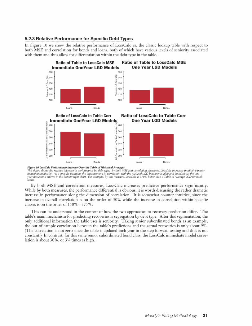
5.2.3 Relative Performance for Specific Debt TypesIn Figure 10 we show the relative performance of LossCalc vs. the classic lookup table with respect toboth MSE and correlation for bonds and loans, both of which have various levels of seniority associatedwith them and thus allow for differentiation within the debt type in the table.

Figure 10 LossCalc Performance Increase Over the Table of Historical AveragesThis figure shows the relative increase in performance by debt type. By both MSE and correlation measures, LossCalc increases predictive perfor-mance dramatically. As a specific example, the improvement in correlation with the realized LGD between a table and LossCalc (at the one-year horizon) is shown in the bottom right chart. For example, by this measure, LossCalc is 370% better than a Table of Average LGD for bankloans.

By both MSE and correlation measures, LossCalc increases predictive performance significantly.While by both measures, the performance differential is obvious; it is worth discussing the rather dramaticincrease in performance along the dimension of correlation. It is somewhat counter intuitive, since theincrease in overall correlation is on the order of 50% while the increase in correlation within specificclasses is on the order of 150% - 375%.

This can be understood in the context of how the two approaches to recovery prediction differ. Thetable's main mechanism for predicting recoveries is segregation by debt type. After this segmentation, theonly additional information the table uses is seniority. Taking senior subordinated bonds as an example,the out-of-sample correlation between the table's predictions and the actual recoveries is only about 9%.(The correlation is not zero since the table is updated each year in the step forward testing and thus is notconstant.) In contrast, for this same senior subordinated bond class, the LossCalc immediate model corre-lation is about 30%, or 3¼ times as high.


100

110

120

130

140

150

Ratio of Table to LossCalc MSE Immediate OneYear LGD Models

Tab

le v

s. L

C E

rror

(%)

Loans Bonds Loans Bonds

Loans BondsLoans Bonds

100

110

120

130

140

150

Ratio of Table to LossCalc MSE One Year LGD Models

Tab

le v

s. L

C E

rror

(%)

300

320

340

360

380

400

Ratio of LossCalc to Table Corr Immediate OneYear LGD Models

LC C

orre

latio

n vs

Tab

le C

orre

latio

n (%

)

300

320

340

360

380

400

Ratio of LossCalc to Table Corr One Year LGD Models

LC C

orre

latio

n vs

Tab

le C

orre

latio

n (%

)

Thus, the historical table focuses primarily on the between-group (debt type and seniority) variabilityrather than the within group instrument and firm specific variability in recoveries. In contrast, LossCalc'suse of additional information beyond two-way conditioning allows it to incorporate both within- andbetween-group variability more completely. Thus, the improvement in correlation is a reflection of thetypically very low correlation of the table once we narrow the analysis down to the individual rows or cellsin an historical table.

5.2.4 Prediction of Larger Than Expected LossesBy both the MSE and correlation measures, LossCalc out-performs the alternative approaches. However,in addition to concerns about accuracy, many investors and lendors are downside averse: they are mostconcerned about model error when losses are more severe than estimated. The final test of model predic-tive performance that we report here was motivated by this observation.

The test was designed to evaluate each model's ability to predict cases in which actual losses weregreater than historical expectations.

The test proceded as follows:

1. Using the most recent information available up to the time of a default, we first labeled each recordwith repsect to whether the actual loss experienced was greater or less than the historical mean lossfor all instruments to date.

2. We then ordered all out-of-sample predictions for each model from largest predicted loss to small-est predicted loss.

3. Finally, we calculated the percentage of larger than average losses each model captured in its order-ing using standard power tests.

This approach allowed us to convert the model performance to a binary measure which in turn allowedus to use familiar metrics and diagnostis such as power curves and power statistics to measure performance.

All things being equal, if a model was powerful at predicting larger than average losses, we wouldexpect the largest loss predictions to be associated with the actual above average losses and the lowest losspredictions to be associated with below average losses. (On a power curve, this would result in the curvefor a good model being bowed out towards the Northwestern corner of the chart. The random modelwould be a 45° line showing no difference in association between high and low ranked obligations.)While, this metric coarsens somewhat the acutal model output, we have found that it provides a valuableperspective in evaluating recovery model performance.

The results of this analysis are shown in the pannels of Figure 11. The figure shows both theCumulative Accuracy Profile (CAP)16 at left and the area under the curves at right. The larger this area,the more accurate the model. In this case, for a perfect model, this area would be 1.0.

The figure shows that both the table and LossCalc models perform considerably better than randomat differentiating high- and low-loss events, but that the LossCalc models outperform the table by a con-siderable margin.17 This relationship persists over both the immediate and one year horizons. The com-parison of areas under the curves confirms this observation.

16 As a technical note, the power curves shown here differ from the CAP plots we typically use to evaluate default models in that onlythe "goods" are shown on the x-axes. This is done to facilitate analysis since there are a large number of "bad" (below average)events. CAP plots and power curves measure the same quantities but present them in different ways. For a detailed discussion ofCAP plots, refer to Sobehart, Keenan, & Stein [2000].

17 Note that tie breaking was not done in this case, so plateaus are still evident in the figures. A plateau indicates two (or more)instruments with the same model score. In principle, if one was a "bad" and the other was not, the ordering of these becomesimportant. These plateaus could be smoothed too so that the estimation was more accurate, although visual inspection suggeststhat the differences would not change the overall conclusions.


Figure 11 Power at Predicting Higher than Average Loss EventsThis figure shows the predictive power of LossCalc relative to the Table of Averages. It is clear that over both the immediate and one year hori-zons, LossCalc has greater power by a significant margin (i.e., its CAP line is further in the upper left corner and its area under the curve isgreater).

5.2.5 Reliability and Width of Confidence IntervalsTo test the reliability of the confidence intervals produced by the models, we examined them along

two dimensions: width and reliability. The average width of a confidence interval provides informationabout the precision and efficiency of the estimate. To the extent that confidence intervals of one modelare narrower than confidence intervals for another model, then this implies that the former predictionsare more reliable. From an economic perspective, it implies more certainty regarding the capital thatmight be required to protect against losses.

However, a CI can be made arbitrarily narrow if one ignores that the counter-balancing constraint isthe reliability of a model's CI at actually predicting the true interval. Said otherwise, if a given model pro-duces an a% confidence interval, then in practice out-of-sample, we would expect to observe actual real-ized losses outside the interval about 1-a% of the time. To the extent that the model experienced anundue number of actual losses outside its "narrow" CI, this would provide evidence that the "narrow" CIwere, in fact, too narrow.

To examine these two dimensions of the CI, we first generated CIs for each model and calibratedthem to in-sample data. We report the average widths of these CI in the first (left) section of Figure 12.We then tested out-of-sample and out-of-time the number of cases in which the actual observed lossesexceeded the predicted interval.

As we discuss below, we examined several methods for CI prediction. Some of these required the use ofactual prediction errors from previous periods. Thus, this type of testing requires more data than accuracytesting. Therefore, we were more limited in the amount of data available for this validation. Nonetheless,we had a large number of recovery observations on which to draw. We chose the period prior to 1998 forestimating the CI and the subsequent period for out-of-sample-out-of-time testing. This resulted in about500 observations for tests at the one-year horizon and close to 600 for the immediate tests.


Model Score% R

ecov

erie

s Lo

wer

than

His

toric

Avg

.

0.0

0.2

0.4

0.6

0.8

1.0

Immediate LGD Models

0.65 0.70 0.75 0.80 0.85

Area under curve

Table of Averages

Table of Averages

LossCalc

Model Score% R

ecov

erie

s Lo

wer

than

His

toric

Avg

.

0.0

0.2

0.4

0.6

0.8

1.0

One Year LGD Models

0.65 0.70 0.75 0.80 0.85Area under curve

LossCalc

Figure 12 The Width and Reliability of Model Confidence IntervalsOf the four charts in this figure, the left two show "width" and the right two show "reliability" of the confidence intervals. In addition, the top twocharts show the Immediate prediction of LGD and the bottom two charts show the One Year prediction. LossCalc has the narrowest averageinterval width (shortest columns) while also maintaining good reliability (horizontal bars that are closest to 20% target.

Figure 12, shows that LossCalc's CIs are more precise (narrower) than both the parametric (standarddeviation) and quantile estimates from the table. However, uneven coverage percentages add some uncer-tainty to the analysis.

For example, for the immediate horizon version of LossCalc, the actual out-of-sample coverage of thehistorical table was higher than LossCalc signalling not only a more precise estimation, but also a moreefficient one. However, the 1-year version shows a slightly higher out-of-sample coverage than the his-torical table indicating that the width of the CI could probably have been made tighter. Similarly, thewidth of the parametric CI for the table are likely optimistically narrow, due to the higher than expectednumber of cases outside the CI. Unfortuately, there is no way to anticipate such variances from theexpected CI a priori.

We can, however, ask the following question: What would the width of the CIs have been if all calcu-lation approaches had the same out-of-sample coverage? This would give some insight into the relativewidth of these confidence bounds after controlling for coverage.

To address this, we adjusted the parameters of the confidence estimates to ensure that coverage of allmethods on the out-of-sample data would be consistent with the LossCalc coverage. This then restrictedthe analysis to the evaluation of the comparative widths of the CI. We stress here that this adjustment wouldnot be possible in practice since it relies on knowledge of the future for calibration of the parameters. We perform ithere only to provide descriptive analysis of the the relative performance of the LossCalc CI. The resultsof this analysis are given in Figure 13. It is clear from the figures that the LossCalc estimates are narrowerthan other alternatives.


60

65

70

75

80

85

90

Mea

n %

CI w

idth

: Ins

tant

aneo

us

Table (pctile) Table (SD) LC (cond)

0 5 10 15 20 25

% losses greater than 80% CI: Immediate LGD Models

60

65

70

75

80

85

90

Mea

n %

con

fiden

ce in

terv

al w

idth

:One

yea

rTable (pctile) Table (SD) LC (cond)

Table (pctile)

Table (SD)

LC (cond)

Table (pctile)

Table (SD)

LC (cond)

0 5 10 15 20 25

% losses greater than 80% CI: One Year LGD Models

Confidence Interval Performance: 80% CI

Figure 13 The Width of Model Confidence Intervals when Coverage is Held ConstantThis figure shows the width of the confidence intervals for the LGD models. LossCalc has the narrowest average interval width even while hold-ing constant the coverage percentage.

6. The DatasetThe primary dataset for LossCalc is Moody's proprietary default and recovery database. This is the samedefault database that Moody's uses in its annual default study. In addition, this information was supple-mented with other types of data such as financial statements and credit indices that allow for a morerefined analysis.

We focus here on the secondary market pricing of defaulted debt as quoted one month after the dateof default. Importantly, we use debt-issue specific market quotes. These prices are not "matrix" prices,which are broad broker-created tables keyed off maturity, credit grade, and instrument type with no par-ticular consideration of the specific issuer.

6.1 HISTORICAL TIME PERIOD ANALYZEDIt is not clear that going back to the extreme limits of the historical record would produce the most usefulmodel. This is because, as with any predictive model, experience that is more recent is likely to be closerin nature and of greater predictive power for the future.

Conversely, we have fewer recovery observations relative to Moody's datasets used for RiskCalc toestimate the probability of default.18 Furthermore, we did not want the model to be overly influenced byany single default event, or even clusters of closely related defaults. This would argue that we should useas much data as possible, which would mean going back far in time.

Two considerations framed our selection of the historical period. First, we felt that the full specifica-tion and validation of our model could only be achieved satisfactorily if one or more (in the case ofLossCalc, two) full economic cycles are included in the dataset. This criterion was motivated by our earlystudies, which found that the credit cycle was a strong determiner of recoveries. Second, our research alsoindicated that firm-level capital structure was also predictive of recovery levels. To tailor our recoveryestimates to the details of specific firms, we deemed it highly desirable to have access to financial state-ment information.

For both of these reasons, the period we used was Jan-1981 to the present. This period covers two fullcredit cycles.

18 By definition, at the obligor level, the number of recovery observations is less than (or equal to) the number of default observations.There cannot be a recovery unless there has been a default observation. By comparison, RiskCalc has far more observations thanLossCalc. However, a single default can also produce several instrument-level recovery observations if the obligor has multipleclasses of debt outstanding.


65

70

75

80

85

Mea

n %

con

fiden

ce in

terv

al w

idth

Table (pctile) Table (SD) LC (cond)Immediate LGD Models

65

70

75

80

85

Mea

n %

con

fiden

ce in

terv

al w

idth

Table (pctile) Table (SD) LC (cond)One Year LGD Models

Confidence Interval Performance: CI Adjusted for Constant Coverage

6.2 SCOPE OF GEOGRAPHIC COVERAGE AND LEGAL DOMAINClearly, bankruptcy laws vary markedly across legal domains. UK law strongly seeks to protect creditors.French law does not recognize the priority of claims of specifically identified security. Some domainsallow creditors to file a petition for insolvency. And this is just a sampling of the diversity of liquidationrules.19 Therefore, for this version of LossCalc, we have chosen to restrict the scope of the model to U.S.debt obligations only.

Having said this, as we move foreword and fit future versions of LossCalc to other domains, we antici-pate that many of our findings will hold.

6.3 SCOPE OF FIRM TYPES AND INSTRUMENT CATEGORIESSeniority standing is especially important to this version of LossCalc because we are focusing exclusivelyon U.S. recoveries. American bankruptcy law applies the concept of the Absolute Priority Rule, which statesthat more senior claimants must be fully satisfied before more junior claimants can start to receive any ofthe defaulted firm's liquidation/reorganization value. In practice, the actions in bankruptcy proceedingare more complicated,20 but this guiding principal makes debt's seniority standing a leading component ofrecovery rate estimation.

Our dataset includes three broad debt instrument types: a) bank loans, b) public bonds, and c) pre-ferred stock. Within loans, there are two seniority grades: "senior secured," which are the more numer-ous, and "senior unsecured." Public bonds subdivide into more seniority classes:

• senior secured;• senior unsecured;• senior subordinated;• subordinated; and• junior subordinated.

In addition to these five broad classes, we break out two specialized classes: corporate mortgages whichare a kind of senior secured bond plus industrial revenue bonds (IRBs), which are a kind of senior unse-cured bond.

Parenthetically, we make no distinction between the different types of preferred stock. In normaltimes, various factors make a real difference in the traded valuations of preferred stock. These include:

• fixed/floating rate payments;• cumulative versus non-cumulative dividends; and• convertibility.

None of these factors above is explicitly mentioned in the bankruptcy code. However, cumulative div-idends may be a strong analogy with accrued interest for bonds, which are included in defaulted debtclaims. As part of our continuing LGD research, we hope to assess whether bankruptcy courts act on this.

As a final detail, we note that in the case of medium term note programs (MTNs), which are charac-terized by a large number of small issues, we consolidate the many individual issues into a single recoveryobservation per default event. The recovery rate realized for this proxy observation is the simple averageof all the individual issuances. It happens that there was never large variability in the recovery estimatesacross issues within a single MTN program.

19 See West & de Bodard [2000a,b,c] and Bartlett [1999].

20 See Mann [1997] for a discussion of the common use and legal treatment of differing seniority classes and Stumpp, et. al. [1977]for a detailing of bank loan structure and collateral.


7. ConclusionIn this report, we described the research done to develop LossCalc, Moody's loss given default (LGD)model. LossCalc is a multi-factor statistical model developed using a database of over 1800 defaultedinstruments. It produces LGD estimates for bonds, syndicated loans, and preferred stock. LossCalcassesses information on four levels of analysis, including the characteristics of the instrument, the capitalstructure of the firm, and macro factors at both the economy and industry level.

The issue of prediction horizon for LGD is one that has not received much attention due to the largelystatic nature of the dominant historical average approach. This implicitly ignores the effects of the creditcycle and other time-varying environmental factors. LossCalc, by its dynamic nature, allows for a muchmore exact specification of LGD horizon and produces estimates on an immediate and one-year horizon.

We conducted extensive out-of-sample out-of-time validation of this model to determine how well itperformed at predicting LGD compared to alternative approaches. The results of this benchmarking showthat the model performs better than common alternatives such as an overall historical average of LGD or atable of average LGDs. LossCalc's performance is superior in terms of both out-of-sample out-of-timeprediction error and correlation of the predictions with actual recovery experience. The model was alsobetter at identifying low recoveries than historical average methods and had fewer large errors.

Since risk management applications place particular demand upon the estimation of parameter uncer-tainty, we have developed a conditional confidence interval prediction approach that results in narrowerconfidence intervals than alternative approaches. In validation testing, these intervals also more accuratelyrepresented the true variability of actual recoveries.

Combining the results of Moody's two models, RiskCalc for default probabilities and LossCalc forrecovery rates, is natural. With this combination, a risk manager can estimate the expected credit losses ofan instrument, given knowledge of the exposure amount. This is a much more complete portrayal ofcredit risk than probability of default alone.

Estimation of the average (mean expected) losses due to credit is commonly used to:

1. set reserve requirements for doubtful accounts;

2. establish minimum pricing levels at which new credit exposures to an obligor may be undertaken;

3. price credit risky instruments such as corporate bonds or credit default swaps; and

4. calculate risk-adjusted performance measures such as RAROC.

LossCalc's estimate of the downside confidence bound of LGD (an 80% two-tailed confidence inter-val) gives greater meaning, consistency, and guidance to stressing recovery rate estimates and for provi-sioning.

LossCalc represents a robust and validated model of United States LGD for the debt types it covers.We believe that this is a productive step forward in answering the call for rigor that the BIS has outlinedin the recently proposed Basel Capital Accord.


Appendix A: Beta Transformation to Normalize Loss DataTo create an approximately normally distributed dependent variable from the raw observations of recov-ery, we first confirmed that defaulted debt valuations were approximately Beta distributed. There is notheoretical reason that this is the "correct" shape of the defaulted debt prices, but previous studies haveconcluded that its characteristics make the Beta a reasonable description of the empirical shape.

Beta-distributions are described in this case by an upper and lower bound and by two shape parame-ters, α and β. Most commonly, it is naturally bounded between zero and one; its mean can be any valuestrictly within its range. The conversion of the Beta distributed recovery values to a more normally distri-bution dependent variable is explicitly defined as follows:

The sub-notation "d" is only used to emphasize that LossCalc fits each debt-type to its own distribution.

Thus, much of the distributions of our three disparate separate asset classes can be captured by specify-ing only two shape parameter values: the α and the β of each Beta-distribution. It is also possible, throughalgebraic manipulation, to specify the Beta-distribution that simply matches the mean and standard devia-tion, which are functions of the shape and boundary parameters.

Mathematically, a Beta-distribution is a function of Gamma distributions. With the lower bound setto zero, the distribution can be described as follows:

The shape parameters can be derived in a variety of ways. For example, the following give them interms of population mean and standard deviation.

Conversely, given Beta-distribution parameters, it is straightforward to calculate the mean and standard deviation.


( )[ ]

( )

{ }stock preferred bonds, loans,

1.0isotherwisebutbonds,for1.1toSet

casesallforzerotoSet

parameter son'DistributiBetaThe

parameter son'DistributiBeta The

valuesmallsomeraterecoveryobserved,min

,,,,1

=====

=−=

== −

d

Max

Min

shape

center

MaxRecovRt

where

MaxMinRecovRtBetadistNYVariableDependant

d

d

d

dddii

βα

εε

βα

−

ΓΓ+Γ==

−−

MaxMax

x

Max

xMaxMinxBeta

11

)()(

)(),0,,,(

11 βα

βαβαβα

( )

−⋅=

−

⋅−⋅⋅= 11

max 2 µαβ

σµµµα Max

andMax

Max

( ) ( ) MaxandMax ⋅++++

⋅=⋅+

=βαβα

βασβα

αµ12

Appendix B: An Overview of the Validation ApproachTo validate the performance of LossCalc, we have used the approach adopted and refined by Moody's andused to validate Moody's quantitative default prediction models (RiskCalc). The approach, termed walkforward validation, is a robust means for ensuring that:

• models have not been "over-fit" to the data;• future performance can be well understood; and• the modeling approach, as well as any individual model produced by it, is robust through time and

credit cycles.

We give only a brief overview of the methodology here; a fuller description is detailed in Sobehart,Keenan, & Stein [2000].21

B.1. CONTROLLING FOR "OVER FITTING" RISK: WALK-FORWARD TESTINGIn order to avoid embedding unwanted sample dependency, we have found it useful to develop and vali-date models using some type of out-of-sample, out-of-universe and out-of-time testing approach on panelor cross-sectional datasets.22 However, such an approach can generate false impressions about reliabilityof a model if done incorrectly. "Hold out" testing can sometimes miss important model problems, partic-ularly when processes vary over time, as credit risk does.23 Dhar & Stein [1997] suggest a framework forframing these issues as well as providing a more detailed discussion and some examples from finance.

Our testing approach is designed to test models in a realistic setting, emulating closely the manner inwhich the models would be used in practice. The procedure we describe is often referred to in the tradingmodel literature as "walk-forward" testing.

The walk-forward procedure works as follows:

1. Select a year, for example, 1991.

2. Fit the model using all the data available on or before the selected year.

3. Once the model's form and parameters are established for the selected period, generate the modeloutputs for all of the firms available during the following year (in this example 1992). Note thatthese are out-of-time and generally out-of-sample.

4. Save the prediction as part of a result set.

5. Now move the window up one year (e.g.: to 1992) so that all the data through that year can be usedfor fitting and the data for the following year can be used for testing.

6. Repeat steps (2) to (5) adding the new predictions to the result set.

Collecting all the out-of-sample and out-of-time model predictions produces a set of model perfor-mances. This validation result set can then be used to analyze the performance of the model in more detail.

Note that this approach simulates, as closely as possible given the limitations of the data, the processby which the model will actually be used in practice. Each year, the model is refit and used to predictrecoveries one year hence. The walk-forward validation process is outlined in Figure 14.

21 Much of what follows was adapted from Sobehart, Keenan, & Stein [2000].

22 A panel dataset contains observations over time on many individuals. A cross sectional dataset contains one observation on many individuals.

23 See, for example, Mensah [1984].


Figure 14 Validation Methodology: End-to-EndWe fit a model using a sample of historical data on recoveries and test the model using data on new recoveries one-year later (upper portion ofexhibit). Dark circles represent data for fitting the model and white circles represent validation data. We perform "walk-forward testing" (bottomleft) by fitting the parameters of a model using data through a particular year, and testing on data from the following year, and then inching thewhole process forward one year. The results of the testing for each validation year are aggregated and then resampled (lower left) to calculateparticular statistics of interest.

Note that this approach has two significant benefits. First, it allows us to get a realistic view of how aparticular model would perform over time. Second, it allows us to leverage to a higher degree the avail-ability of data for validating models. However, before turning to model performance evaluation, it isimportant to note that the result set is itself a sub-sample of the population. Therefore, it might possiblyyield spurious model performance differences based solely on data anomalies. A common approach toaddressing this issue, and one used extensively in our research, is to use one of a variety of resampling tech-niques to leverage the available data and reduce the dependency on the particular sample at hand.24

Unless otherwise noted, all results presented in this study are from out-of-sample-out-of-time walk-forward testing.

B.2. RESAMPLINGIt is important to consider that because of the sparseness of defaults (and thus recoveries) in most creditdata; accuracy statistics may sometimes yield spurious model performance differences based only on dataanomalies. To understand these problems we combine the above performance measures with resamplingtechniques to leverage the available data and reduce the dependency on the particular sample at hand. Atypical resampling technique proceeds as follows. From the result set, a sub-sample is selected at random.The performance measure of interest (e.g., mean squared error of the predictions) is calculated for thissub-sample and recorded. Another sub-sample is then drawn, and the process is repeated. This continuesfor many repetitions until a distribution of the performance measure is established. The distribution ofthese results is then used to calculate the variability of the reported performance measure.

Resampling approaches provide an estimate of the variability around the actual reported model perfor-mance. An example is the standard error. This estimate can then be used to assess the significance ofobserved differences in model performance.

24 For data bootstrap, see Efron & Tibshirani [1993], for randomization tests and cross-validation, see Sprent [1998].


1989 1990 1991 1992 1993 1994 1995 1996 1997 1998 1999

llllll

Training set of firms taken at t0

Validation set of new firms not in training sample and taken at t1

-2 -1 0 1

0.0

0.2

0.4

0.6

Error

-3 -2 -1 0 1 2 3

0.0

0.05

0.10

0.15

0.20

0.25

0.30

Error

-3 -2 -1 0 1 2 3

0.0

0.1

0.2

0.3

0.4

Error

-3 -2 -1 0 1 2 3

0.0

0.1

0.2

0.3

0.4

0.5

Error

Resampling

llllll

Resu

lt Se

t

A

B

A

B

A

B

A

B

A

B

Glossary of TermsAbsolute Priority Rule:

Strictly interpreted, a junior class or creditor cannot receive any value in bankruptcy resolution if themore senior classes have not yet been fully satisfied. This rule guides allocations among creditor class-es concerning a plan of reorganization, but is rarely strictly applied. Commonly, the bankruptcy courtwill give some amount of consideration to lower class creditors and/or to preferred and commonstockholders in order to circumvent objections, delays, and other litigation.

Debt-type or Instrument Type:The form of the credit obligation, (e.g., bank loan, public bond, preferred stock).

Expected Recovery Given Default (ERGD):Recovery, in this context, is the compliment of loss. See, "Recovery Rate."

Loss Given Default (LGD):Typically stated as a percent of the debt's par value, it is one minus the recovery rate. This is the ter-minology used by the BIS. See "Recovery Rate."

Loss in the Event of Default (LIED): See "Loss Given Default."

Normalization:Variables can be characterized by their central tendency (average), volatility (standard deviation),skewness (tendency to bunch up towards one end of its range), etc. These measures help describe thevariable's shape or distribution. For many observations in nature, variables have a bell-shaped (a.k.a.,Normal or Gaussian) distribution. If a variable is not normally distributed, a transformation can typi-cally be devised that will convert it to be Normal. An inverse of this transformation would reverse theeffect. This sort of transformation is termed Normalization.

Priority of Claims:A plan must classify claims into "substantially similar" groups known as "classes." Classification ofclaims reflects differences in the rights of creditors that call for a difference in treatment. Not allclaims that are "substantially similar" need be placed in the same class, but those that are placed in thesame class must be alike. Unsecured creditors are frequently classified together, whereas each securedclaim is generally classified separately. Claims within each class must be treated equally, and a planmust not unfairly discriminate between creditors (whether or not classified together) of equal priority.

Recovery Rate:The value that a creditor would receive in satisfaction of the claims on a defaulted credit. LossCalcstates this as a percentage of the debt's par value, which is the most common practice. An alternativedefinition, which is common in the reduced form models,25 is to state recovery as a percentage of mar-ket value. This definition is more tractable, but is not well aligned with creditor's true claims in default.

Seniority Class: We use this term to include seniority grades across all debt-types. In a bankruptcy proceeding, all creditobligations of a firm are assigned to a seniority class and the classes are ranked by their seniority standing.In an idealized example, all claims in the highest seniority class would be satisfied before claims belowthem. Applying the Absolute Priority Rule in a kind of "stair-step" or "water fall" does this.

Seniority Grade:Within an instrument type (e.g., public bonds) there is often distinction in seniority such as betweensecured vs. unsecured or senior vs. subordinated.

25 See Gurdip, Madan & Zhang [2001], Jarrow [2001] and Unal, Madan & Guntay [2000].


Bibliography1. Altman, E. I. (1998). "Market Dynamics and Investment Performance of Distressed and Defaulted Debt

Securities." New York University Salomon Center. (http://www.stern.nyu.edu/clb/papers.html#MARKET)

2. Altman, E. I. and A. C. Eberhart (1994). "Do Seniority Provisions Protect Bondholders' Investments?"Journal of Portfolio Management. Summer: 67-75.

3. Altman, E. I. and V. M. Kishmore (1996). "Almost Everything you Wanted to Know about Recoverieson Defaulted Bonds." Financial Analysis Journal. November/December: 56-62.

4. Andrade, G. and S. Kaplan (1998). "How Costly is Financial (Not Economic) Distress? Evidence fromHighly Leveraged Transactions that Became Distressed." Journal of Finance. Vol. LIII. 4: 1443-1494.

5. Asarnow, E. and D. Edwards (1995). "Measuring Loss on Defaulted Bank Loans: A 24-Year Study."Journal of Commercial Lending. March. Vol. 77.7: 11-23.

6. Asquith, P., R. Gertner and D. Scharfstein (1994). "Anatomy of Financial Distress: An Examination ofJunk-Bond Issuers." Quarterly Journal of Economics. August: 625-657.

7. Bakshi, G., D. Madan and F. Zhang (2001). "Recovery in Default Risk Modeling: TheoreticalFoundations and Empirical Applications." University of Maryland and the Federal Reserve Board.

8. Barclay, M. J. and C. W. Smith (1995). "The Priority Structure of Corporate Liabilities." Journal ofFinance. Vol. L. 3: 899-917.

9. Bartlett, F. (1999). "Regimes, Recoveries and Loan Ratings: the importance of insolvency legislation."Fitch/IBCA - Loan Products. (http://www.defaultrisk.com/pp_recov_12.htm)

10. Basel Committee on Banking Supervision (2001). "The New Basel Capital Accord." Bank forInternational Settlements. (http://www.bis.org/publ/bcbsca.htm)

11. Bester, H. (1994). "The Role of Collateral in a Model of Debt Renegotiation." Journal of Money, Creditand Banking. Vol. 26. 1: 72-86.

12. Borenstein, S. and N. L. Rose (1995). "Do Airlines in Chapter 11 Harm Their Rivals?: Bankruptcyand Pricing Behavior in U.S. Airline Markets." National Bureau of Economic Research.

13. Carty, L., D. Lieberman and J. S. Fons (1995). "Corporate Bond Defaults and Default Rates 1970-1994." Moody's Investors Service. (http://riskcalc.moodysrms.com/us/research/defrate.asp)

14. Carty, L. V. (1998). "Bankrupt Bank Loan Recoveries." Moody's Investors Service.(http://riskcalc.moodysrms.com/us/research/lied.asp)

15. Carty, L. V. and D. Lieberman (1996). "Defaulted Bank Loan Recoveries." Moody's Investors Service.(http://riskcalc.moodysrms.com/us/research/lied.asp)

16. Chatterjee, S., U. S. Dhillon and G. G. Ramirez (1996). "Resolution of Financial Distress: DebtRestructurings via Chapter 11, Prepackaged Bankruptcies, and Workouts." Financial Management.Vol. 25. 1: 5-18.

17. Dhar, V. and R. Stein (1998). "Finding Robust and Usable Models with Data Mining: Examples fromFinance." PCAI.

18. Eales, R. and E. Bosworth (1998). "Severity of Loss in the Event of Default in Small Business andLarger Consumer Loans." The Journal of Lending and Credit Risk Management. May: 58-65.

19. Eberhart, A. C., E.I. Altman and R. Aggarwal (1999). "The Equity Performance of Firms Emergingfrom Bankruptcy." Journal of Finance. Vol. LIV. 5: 1855-1868.

20. Eberhart, A. C. and R. J. Sweeney (1992). "Does the Bond Market Predict Bankruptcy Settlements?"Journal of Finance. Vol. XLVII. 3: 943-980.

21. Efron, B. and R. J. Tibshirani (1993). An Introduction to the Bootstrap (Monographs on Statistics andApplied Probability, No. 57). Chapman and Hall/CRC Press.

22. Falkenstein, E., A. Boral and L. V. Carty (2000). "RiskCalc For Private Companies: Moody's DefaultModel." Moody's Risk Management. (http://riskcalc.moodysrms.com/us/research/crm.asp)

23. Fridson, M. S. (2000). "Recovery Trends: Any Usefulness Whatsoever?" Merrill Lynch - GlobalSecurities Research and Economics Group. (http://www.defaultrisk.com/pp_recov_13.htm)


24. Fridson, M. S., M. C. Garman and K. Okashima (2000). "Recovery Rates: The Search for Meaning."Merrill Lynch - Global Securities Research and Economics Group.

25. Frye, J. (2000). "Depressing Recoveries." Federal Reserve Bank of Chicago.(http://www.chicagofed.org/publications/publicpolicystudies/emergingissues/authorF.cfm)

26. Gilson, S. C., E. S. Hotchkiss and R. S. Ruback (2000). "Valuation of Bankrupt Firms." HarvardBusiness School and Boston College. (http://www2.bc.edu/~hotchkis/)

27. Gupton, G. M., C. C. Finger and M. Bhatia (1997). "CreditMetrics—Technical Document." J.P.Morgan. (http://www.creditmetrics.com)

28. Gupton, G. M., D. Gates and L. V. Carty (2000). "Bank Loan Loss Given Default." Moody's RiskManagement. (http://riskcalc.moodysrms.com/us/research/lied.asp)

29. Gupton, G. M. and R.M. Stein (2001). "A Matter of Perspective." Credit. Vol 2.9: 22-23. (http://www.creditmag.com)

30. Hamilton, D. T. (1999). "Monthly Default Report." Moody's Investors Service.(http://www.moodysqra.com/research/mdr.asp)

31. Hamilton, D. T. and A. Berthault (2000). "The Investment Performance of Bankrupt Corporate DebtObligations: Moody's Bankrupt Bond Index 2000." Moody's Investors Service.(http://riskcalc.moodysrms.com/us/research/mbbi.asp)

32. Hamilton, D. T. and L. V. Carty (1999). "Debt Recoveries for Corporate Bankruptcies." Moody'sRisk Management. (http://riskcalc.moodysrms.com/us/research/lied.asp)

33. Hamilton, D. T., G. M. Gupton and A. Berhault (2001). "Default and Recovery Rates of CorporateBond Issuers: 2000." Moody's Risk Management.(http://riskcalc.moodysrms.com/us/research/defrate.asp)

34. Hege, U. and P. Mella-Barral (1999). "Collateral, Renegotiation and the Value of Diffusely HeldDebt." Tilburg University. (http://econpapers.hhs.se/paper/dgrkubcen/199994.htm)

35. Helwege, J. (1999). "How Long Do Junk Bonds Spend in Default?" Journal of Finance. Vol. LIV. 1:341-457.

36. Indro, D. C., R. T. Leach and W. Y. Lee (1999). "Sources of Gains to Shareholders from BankruptcyResolution." Journal of Banking and Finance. Vol. 23. 1: 21-47.(http://www.elsevier.nl/homepage/sae/econbase/jbf/)

37. Izvorski, I. (1997). "Recovery Ratios and Survival Times for Corporate Bonds." InternationalMonetary Fund.

38. James, C. (1991). "The Losses Realized in Bank Failures." Journal of Finance. Vol. XLVI. 4: 1223-1242.

39. Jarrow, R. (2001). "Default Parameter Estimation Using Market Prices." Financial Analysts Journal.Vol. 57. 5: 75-92.

40. Jokivuolle, E. and S. Peura (2000). "A Model for Estimating Recovery Rates and Collateral Haircutsfor Bank Loans." Bank of Finland and Leonia plc. (http://www.iue.it/FinConsEU/literature.htm)

41. Keenan, S. C., D. T. Hamilton and A. Berthault (2000). "Historical Default Rates of Corporate BondIssuers, 1920-1999." Moody's Risk Management.(http://riskcalc.moodysrms.com/us/research/defrate.asp)

42. Longhofer, S. D. (1997). "Absolute Priority Rule Violations, Credit Rationing, and Efficiency."Journal of Financial Intermediation. Vol. 6. 3: 249-267. (http://webs.twsu.edu/longhofer)

43. Longhofer, S. D. and C. T. Carlstrom (1995). "Absolute Priority Rule Violations in Bankruptcy."Economic Review: 21-30. (http://webs.twsu.edu/longhofer)

44. Longhofer, S. D. and J. A. C. Santos (2000). "The Importance of Bank Seniority for RelationshipLending." Journal of Financial Intermediation. Vol. 9. 1: 57-89. (http://webs.twsu.edu/longhofer)

45. Longhofer, S. D. and J. A. C. Santos (2001). "The Paradox of Priority." Wichita State University.(http://webs.twsu.edu/longhofer)

46. Mann, R. J. (1997). "Explaining the Patterns of Secured Credit." Harvard Law Review. Vol. 110. 3: 625-683.


47. Mella-Barral, P. (1999). "The Dynamics of Default and Debt Reorganization." The Review of FinancialStudies. Vol. 12. 3: 535-578. (http://rfs.oupjournals.org/)

48. Mensah, Y. M. (1984). "An Examination of the Stationarity of Multivariate Bankruptcy PredictionModels: A Methodological Study." Journal of Accounting Research. Vol. 22. 1: 380-395.

49. Merrick Jr., J. J. (2001). "Crisis Dynamics of Implied Default Recovery Ratios: Evidence from Russiaand Argentina." New York University. (http://www.udesa.edu.ar/lames2001/Program1.htm)

50. Noe, T. H. and M. J. Rebello (1996). "Feasting on a Corporate Carcass: Bluffing, Bondmail, andReputation in the Market for Distressed-Firm Debt." Tulane University and Georgia StateUniversity. (http://freeman.sob.tulane.edu/freeman/faculty/tnoe.htm)

51. Pulvino, T. C. (1999). "Effects of Bankruptcy Court Protection on Asset Sales." Journal of FinancialEconomics. Vol. 52. 2: 151-186.

52. RiskMetrics (1996). "RiskMetrics—Technical Document." J.P. Morgan.(http://www.riskmetrics.com)

53. Simonoff, J. S. (1996). Smoothing Methods in Statistics. Springer Verlag.

54. Sobehart, J., S. Keenan and R. Stein (2000). "Validation methodologies for default risk models."Credit: 51-56. (http://riskcalc.moodysrms.com/us/research/papers.asp

55. Sobehart, J. R., S. C. Keenan and R. M. Stein (2000). "Benchmarking Quantitative Default RiskModels: A Validation Methodology." Moody's Risk Management.(http://riskcalc.moodysrms.com/us/research/crm.asp)

56. Sobehart, J. R. and R. M. Stein (2000). "Moody's Public Firm Risk Model: A Hybrid Approach ToModeling Short Term Default Risk." Moody's Risk Management.(http://riskcalc.moodysrms.com/us/research/crm.asp)

57. Sprent, P. (1998). Data Driven Statistical Methods. Chapman-Hall/CRC Press.

58. Stumpp, P., T. Marshela, M. Mulvaney, et al. (1997). "A Sense of Security: Moody's Approach toEvaluating Bank Loan Structure and Collateral." Moody's Investors Service.(http://www.moodys.com)

59. Swank, T. A. and T. H. Root (1995). "Bonds in Default: Is Patience a Virtue?" Journal of Fixed Income.June: 26-31.

60. Thorburn, K. S. (1999). "Bankruptcy Auctions: Costs, Debt Recovery, and Firm Survival." Derivedfrom Doctoral Thesis Dartmouth College. (http://www.defaultrisk.com/pp_recov_09.htm)

61. Unal, H., D. Madan and L. Guntay (2001). "A Simple Approach to Estimate Recovery Rates withAPR Violation from Debt Spreads." University of Maryland.(http://www.mbs.umd.edu/Finance/hunal/papers.html)

62. Wagner III, H. S. (1996). "The Pricing of Bonds in Bankruptcy and Financial Restructuring." TheJournal of Fixed Income. June: 40-47.

63. Ward, D. J. and G. L. Griepentrog (1993). "Risk and Return in Defaulted Bonds." Financial AnalystsJournal. May/June : 61-65.

64. Welch, I. (1997). "Why is Bank Debt Senior? A Theory of Asymmetry and Claim Priority Based onInfluence Costs." The Review of Financial Studies. Vol. 10. 4: 1203-1236. (http://rfs.oupjournals.org/)

65. West, M. and E. de Bodard (2000). "Bankruptcy and Ratings: A Leveraged Finance Approach forEurope." Moody's Investors Service. (http://www.moodys.com)

66. West, M. and E. de Bodard (2000). "Bankruptcy and Ratings: A Leveraged Finance Approach forEurope - Part II: France." Moody's Investors Service. (http://www.moodys.com)

67. West, M. and E. de Bodard (2000). "Bankruptcy and Ratings: A Leveraged Finance Approach forEurope - Part III: Germany." Moody's Investors Service. (http://www.moodys.com)


LossCalc

: M

oody’s

Model fo

r Pre

dic

ting L

oss G

iven D

efa

ult

(LG

D)

To order reprints of this report (100 copies minimum), please call 1.212.553.1658.Report Number: 73568

Specia

l Com

ment

Documents

LossCalcTM: Moody’s Model for Predicting Loss Given ... · This report describes and documents LossCalc, Moody's model for predicting loss given default ... bonds, and preferred