LAURO MOSCARDINI!DIP. FISICA E ASTRONOMIA, UNIBO!LAURO.MOSCARDINI@UNIBO.IT!

Looking for Baryon Acoustic Oscillations of

Galaxy Clusters

Hot spots in the XMM sky, Mykonos, 15th-18th June 2016

In collaboration with A. Veropalumbo, F. Marulli, M. Moresco & A. Cimatti see Veropalumbo et al. 2014, MNRAS, 442, 3275 and Veropalumbo et al., 2016, MNRAS, 458, 1909

The era of !high-precision Cosmology

Different cosmological probes are converging towards the so-call concordance model: the flat ΛCDM model

•  a flat Universe: Ωk=1-ΩM-ΩΛ=0 •  a small baryonic component: Ωb≈5%

•  a dominant dark energy component in the form of a cosmological constant Λ Planck Collaboration

The era of !high-precision Cosmology

The concordance cosmological model received a strong support from the recent analysis of Cosmic Microwave Background data by Planck.

Constraining !the cosmological parameters

H z( ) = H0 ΩM 1+ z( )3 +ΩDE 1+ z( )3 1+w( ) +Ωk 1+ z( )2⎡⎣

⎤⎦1/2≡ H0E z( )

We measure the main cosmological parameters through their effects on the expansion of the Universe: from the Friedmann equations we can derive how the Hubble parameter H(z) varies with redshift:

An example for flat cosmologies

Constraining !the cosmological parameters

Different approaches are now available: •  standard candles - measurements of dL (an integral of H(z)-1): SNIa, GRB, … •  standard rulers - measurements of dA (an integral of H(z)-1): BAOs •  standard shapes - deformations from perfect circles: Alcock-Paczynski test •  standard clocks - measurement of the age of the Universe t(z) (integral of H(z)-1):

cosmic chronometers, like massive and passive galaxies •  growth of fluctuations - in GR it depends on an integral of a (different) function of

H(z). Crucial for testing modified gravity: CMB, clustering of cosmic structures, weak lensing, cluster counts and clustering, redshift-space distortions, etc.

Standard cosmic rulers The idea is based on the assumption that there is an object whose physical length is known as a function of redshift. By measuring the angle (Δθ) subtended by this ruler (Δχ) as a function of redshift we map out the angular diameter distance dA:

Δθ =ΔχdA z( )

dA z( ) =dL z( )1+ z( )2

∝d ʹzH ʹz( )0

z

∫

By measuring the redshift interval (Δz) associated with this distance we can derive the Hubble parameter H(z):

cΔz = H z( )Δχ

Standard cosmic rulers

What are the properties of !an ideal standard cosmic ruler?

We must be able •  to calibrate it accurately over most of the age of the universe •  to measure it over much of the volume of the universe •  to measure it in a very precise way è  there are not cosmic objects having these properties, because

of their non-linear (complex) evolution è  look for something coming from well-known physical

processes happened in the early universe and observable in the distribution of cosmic objects on very large scale (because easier to be modeled)

è  the baryon acoustic oscillations of the Cosmic Microwave Background

Sound waves in the early Universe •  At early times the universe was hot, dense and ionized. Photons and matter were

tightly coupled by Thomson scattering (fluid approximation). •  Initial fluctuations in density and gravitational potential drive acoustic waves in

the baryon-photon fluid with sound speed cs: compressions and rarefactions. •  These show up as temperature fluctuations in the CMB. •  There is also a component due to the velocity of the fluid: the Doppler effect. •  A sudden “recombination” decouples the radiation and matter, giving us a

snapshot of the fluid at “last scattering”.

•  These fluctuations are then projected on the sky with λ~rlsθ or l~krls.

Our cosmic ruler: the CMB BAOs! First “compression”, at kcstls=π. Max. density, null velocity

Max. velocity

First “rarefaction” peak at kcstls=2π

Acoustic scale is set by the sound horizon at last scattering rs(zls): Planck measured it accurately!

rs zls( ) =cs z( )H z( )zls

∞

∫ dz =147.34± 0.65Mpc

•  It can be calibrated accurately over most of the age of the universe.

•  It can be measured over much of the volume of the universe in a very precise way.

•  It is due to well-known physical processes happened in the early universe and observable in the distribution of cosmic objects on very large scale (because easier to be modeled)

Our cosmic ruler: the CMB BAOs! First “compression”, at kcstls=π. Max. density, null velocity

Max. velocity

First “rarefaction” peak at kcstls=2π

Acoustic scale is set by the sound horizon at last scattering rs(zls): Planck measured it accurately!

rs zls( ) =cs z( )H z( )zls

∞

∫ dz =147.34± 0.65Mpc

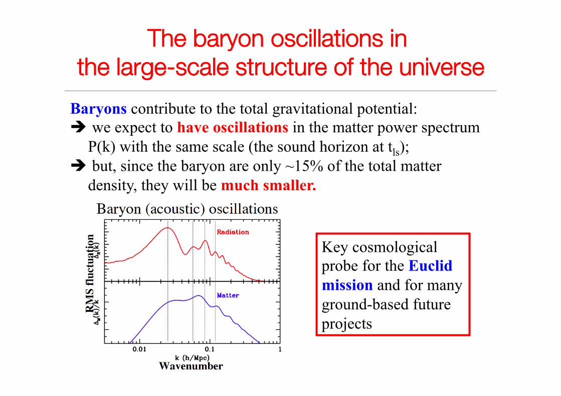
The baryon oscillations in !the large-scale structure of the universe

Baryons contribute to the total gravitational potential: è  we expect to have oscillations in the matter power spectrum

P(k) with the same scale (the sound horizon at tls); è  but, since the baryon are only ~15% of the total matter

density, they will be much smaller.

Key cosmological probe for the Euclid mission and for many ground-based future projects

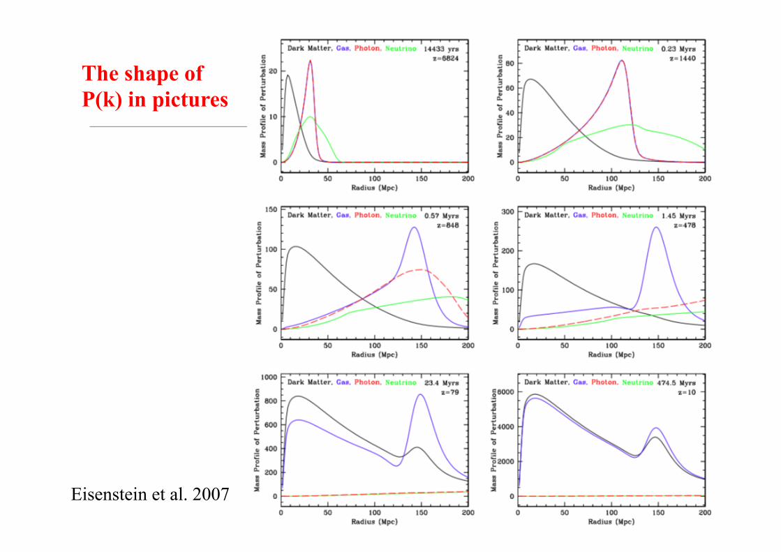
The shape of P(k) in pictures

Eisenstein et al. 2007

The BAO signatures !in the clustering signals

A damped, almost harmonic sequence of small “wiggles” (<10%) in the matter power spectrum

An acoustic feature (ξ≈0.02) at ~100 Mpc/h with width ~10 Mpc/h in the two-point correlation function

An example of application: !BAOs in the SDSS BOSS DR11

Shape and position of the BAO peak is influenced by non linear growth of structures: reconstruction of the density field improves the distance constraint.

The BAO signatures in the clustering signals:!an example in the SDSS BOSS

Shape and position of the BAO peak is influenced by non linear growth of structures: reconstruction of the density field improves the distance constraint.

A damped, almost harmonic sequence of small “wiggles” (<10%) in the matter power spectrum.

An acoustic feature (ξ≈0.02) at ~100 Mpc/h with width ~10 Mpc/h in the two-point correlation function.

A summary of the BAO results

Aubourg et al. 2014

Cosmological constraints! from BAOs

Aubourg et al. 2014

Cosmology with Galaxy Clusters Galaxy clusters are an extremely powerful cosmological probe: •  Mass function è cosmological parameters, dark energy models

(ΩΛ,w0,wa), neutrino mass, modified gravity, … •  Baryon fraction è Ωb •  Matter density profiles è constraints on modified gravity and

dark matter properties •  Mass-concentration relation è cosmological constraints •  X-ray-SZ-lensing observations è constraints using DA(z) •  Clustering properties è growth of structures, cosmological

parameters, tests of GR, …

Why using Galaxy Clusters !for BAO studies?

Galaxy Clusters represent the highest peaks in the matter density field

•  They are more clustered than galaxies:

è Higher clustering signal

•  They are less affected by non-linear dynamics: è No Fingers of God

•  They are sparser than other tracers:

è Larger error bars in the correlation function

PROs CONs

The catalogues of galaxy clusters •  Sample of ~130000 galaxy clusters (Wen, Han, Liu 2012) identified applying FoF on the

photometric sample of SDSS DR8 •  Area of 15000 deg2, covering 0.1< z < 0.6 •  Cluster center è BCG angular coordinates + mean members photometric redshift •  Mcl≥ 6 1013 M¤ (from weak lensing scaling relation)

The catalogues of galaxy clusters •  Sample of ~130000 galaxy clusters (Wen, Han, Liu 2012) identified applying FoF on the

photometric sample of SDSS DR8 •  Area of 15000 deg2, covering 0.1< z < 0.6 •  Cluster center è BCG angular coordinates + mean members photometric redshift •  Mcl≥ 6 1013 M¤ (from weak lensing scaling relation) •  Spectroscopic redshift from SDSS DR12, assigned to a cluster if observed for the BCG

The galaxy cluster samples

Measuring !the two-point correlation function We use the Landy & Szalay (1993) estimator:

ξ̂ r( ) =1+ NRR

NDD

DD r( )RR r( )

− 2 NRR

NDR

DR r( )RR r( )

The covariance matrix has been estimated using mock data or internal subsampling techniques (jackknife and/or bootstrap).

CosmoBolognaLib

CosmoBolognaLib!(Marulli, Moresco, Veropalumbo 2016, arXiv:1511.00012)

C++, Python libraries aimed at defining a common numerical environment for cosmological investigations of the large-scale structure of the Universe. Fully documented and publicly available: •  GitHub depository: https://github.com/federicomarulli/CosmoBolognaLib •  Tar file and documentation: http://apps.difa.unibo.it/files/people/federico.marulli3/CosmoBolognaLib/

Measuring !the two-point correlation function

CosmoBolognaLib!(Marulli, Moresco, Veropalumbo 2016,

arXiv:1511.00012) C++, Python libraries aimed at defining a common numerical environment for cosmological investigations of the large-scale structure of the Universe. Fully documented and publicly available: •  GitHub depository: https://github.com/federicomarulli/CosmoBolognaLib

Landy & Szalay (1993) estimator: ξ̂ r( ) =1+ NRR

NDD

DD r( )RR r( )

− 2 NRR

NDR

DR r( )RR r( )

Measuring !the two-point correlation function Problem: two kinds of distortions affect the measurement: •  Geometrical distortions: consequence of assuming a fiducial

cosmology to transform angular coordinates and redshift in physical cartesian coordinates:

dV = 1+ z( )2 DA2 z( ) cz

H z( )dΩdz ≡ DV

3dΩdz

Correcting for !the geometrical distortions

s→ ys ≡s

DVfid z( )

Sanchez et al. 2012

DV is called isotropic volume distance

Measuring !the two-point correlation function Problem: two kinds of distortions affect the measurement: •  Geometrical distortions: consequence of assuming a fiducial

cosmology to transform angular coordinates and redshift in physical cartesian coordinates:

•  Dynamical distortions: the line-of-sight component of the peculiar velocity perturbs the cosmological redshift of the cosmic object:

dV = 1+ z( )2 DA2 z( ) cz

H z( )dΩdz ≡ DV

3dΩdz

zobs = zc +v||c1+ zc( )

Dynamical distortions

2dFGRS (Peacock et al. 2001); galaxies @ z≤0.2

VIPERS (de la Torre et al. 2013); galaxies @ z~0.8

The redshift-space two-point correlation function of galaxy clusters

60 80 100 120 140 160 180s [Mpc h�1]

�0.01

0.00

0.01

0.02

0.03

0.04

x(s

)

Main GCSN = 12910z = 0.2

60 80 100 120 140 160 180s [Mpc h�1]

0.00

0.01

0.02

0.03

0.04

0.05

0.06

0.07

x(s

)

LOWZ GCSN = 42115z = 0.3

60 80 100 120 140 160 180s [Mpc h�1]

0.00

0.02

0.04

0.06

0.08

x(s

)

CMASS GCSN = 11816z = 0.5

bias=2.00±0.05 bias=2.42±0.02 bias=3.05±0.07

Error bars from lognormal mocks; shaded area represents 68% posterior uncertainties provided by the MCMC analysis

Covariance matrix Crucial ingredient for clustering analysis: necessary for the Gaussian likelihood in the Monte Carlo Markov Chain technique. Computed with 3 different approaches: two internal (jackknife and bootstrap, one external (lognormal mocks).

Ci, j =1

Nreal. −1ξik − ξ̂i( )

k=1

Nreal .

∑ ξ jk − ξ̂ j( )

Modelling the !two-point correlation function

ξ s( ) = b2ξDM αs( )+ A0r2+A1r+ A2

The cluster redshift-space correlation function is assumed to follow the model proposed by Anderson et al. (2012):

Modelling the !two-point correlation function

ξ s( ) = b2ξDM αs( )+ A0r2+A1r+ A2

The cluster redshift-space correlation function is assumed to follow the model proposed by Anderson et al. (2012):

b ç bias parameter between clusters and DM (including the effect of redshift distortions) α ç parameter entirely containing the distance information, then used to put constraints on the cosmological parameters A0,A1,A2 ç parameters of an additive polynomial used to marginalise over signals caused by systematics not fully accounted for

Modelling the !two-point correlation function

PDM k( ) = Plin k( )−Pnw k( )⎡⎣ ⎤⎦exp −k2ΣNL2 / 2( )+Pnw k( )

The DM power spectrum is modeled using the de-wiggled template (Einsenstein et al. 2007)

Plin ç linear power spectrum (from CAMB) Pnw ç power spectrum without the BAO features (Eisenstein & Hu 1998) ΣNL ç parametrizes the non-linear broadening of the BAO peak The DM correlation function is simply the Fourier Transform of the DM power spectrum:

ξDM r( ) = 12π 2 k2∫ PDM k( )

sin kr( )kr

dk

Modelling the !two-point correlation function

PDM k( ) = Plin k( )−Pnw k( )⎡⎣ ⎤⎦exp −k2ΣNL2 / 2( )+Pnw k( )

The DM power spectrum is modeled using the de-wiggled template (Einsenstein et al. 2007)

Plin ç linear power spectrum (from CAMB) Pnw ç power spectrum without the BAO features (Eisenstein & Hu 1998) ΣNL ç parametrizes the non-linear broadening of the BAO peak

Wiggled/De-wiggled !Power Spectrum

BAO distance constraint The distance constraint is entirely contained in α. It is necessary to correct for the geometric distortions introduced by the assumption of a fiducial cosmology to compute the two-point correlation:

DV z( ) ≡ 1+ z( )2 DA2 z( ) cz

H z( )

⎡

⎣⎢⎢

⎤

⎦⎥⎥

1/3

=αDV

fid

rsfid ⋅ rs

Two possible methods: •  Calibrated, when one assumes that the true value of the

sound horizon is known from CMB (i.e. Planck) •  Uncalibrated, when one prefer to use Dv(z)/rs

Significance of !the BAO detection

0 20 40 60 80 100SNL [Mpc · h�1]

0

2

4

6

8

10

12

Dc

2

1s

2s

3s

Main-GCS

LogNormalJackknifeBootstrap

0 20 40 60 80 100SNL [Mpc · h�1]

0

2

4

6

8

10

12

Dc

2

LOWZ-GCS

0 20 40 60 80 100SNL [Mpc · h�1]

0

2

4

6

8

10

12

Dc

2

CMASS-GCS

α

DV z( ) ≡ 1+ z( )2 DA2 z( ) cz

H z( )

⎡

⎣⎢⎢

⎤

⎦⎥⎥

1/3

=αDV

fid

rsfid ⋅ rs

0.1 0.2 0.3 0.4 0.5 0.6 0.7

z

500

1000

1500

2000

DV(z

)(rfi

ds

/rs)

Mpc

/h

Planck cosmologyWM = 1, WL = 0WM = 0, WL = 1

Main-GCSLOWZ-GCSCMASS-GCS6dFGSMGSLOWZWIGGLEzCMASS

Distance constraints

Cosmological constraints: ΛCDM model

Flat universe: Ωk =1- ΩM-ΩΛ=0 Dark energy with eq. of state parameter w=-1 è cosmological constant Λ

H 2 z( ) = H02 ΩM 1+ z( )3 +ΩΛ⎡⎣

⎤⎦

H0 = 64−8+17 kms ⋅Mpc

ΩM = 0.33−0.16+0.24

Cosmological constraints: oΛCDM models

H 2 z( ) = H02 ΩM 1+ z( )3 +ΩΛ +Ωk 1+ z( )2⎡⎣

⎤⎦

Non-flat universe: Ωk =1- ΩM-ΩΛ≠0 Dark energy with eq. of state parameter w=-1 è cosmological constant Λ

H0 = Ν 67,20( ) kms ⋅Mpc

Ωk = −0.01−0.33+0.34

The Planck cosmology is compatible with the cluster BAO results

BAO: Galaxies vs. Clusters

BGCs at the centre of galaxy clusters are a (small) subsample of the whole BOSS galaxy catalogue. What are the differences in their clustering properties and in the strength of the BAO signal?

BAO: Galaxies vs. Clusters

•  Clear difference in the bias è galaxy cluster centre (BCGs) are not a random subsample of the whole galaxy population

•  BAO peak very clear in the cluster correlation function despite of the largest measurement errors

BAO: Galaxies vs. Clusters

The peculiar velocity term in the observed redshift generates the Fingers of God. These distortions have influences on the BAO scale too.

zobs = zc +v||c1+ zc( )

Conclusions •  We computed the two-point correlation function for

galaxy clusters at three different redshifts. •  We showed that BAO distance constraints from galaxy

cluster clustering are possible! •  They have a competitive precision w.r.t. galaxy

clustering BAO constraints. •  Cluster clustering shows differences in bias, FoG, NL

w.r.t. galaxy clustering •  We derive cosmological constraints from distance

redshift relation for a set of different cosmological scenarios.

•  The results for cluster BAO can be used in combination with other cluster probes (like the mass function)

Cosmological constraints: wCDM models

Flat universe: Ωk =1- ΩM-ΩDE=0 Dark energy with generic eq. of state parameter w

H 2 z( ) = H02 ΩM 1+ z( )3 +ΩDE 1+ z( )3 1+w( )⎡⎣

⎤⎦

H0 = Ν 67,20( ) kms ⋅Mpc

ΩM = 0.38−0.14+0.21

w = −1.06−0.52+0.49

Cosmological constraints: owCDM models

Non-flat universe: Ωk =1- ΩM-ΩDE≠0 Dark energy with generic eq. of state parameter w

H 2 z( ) = H02 ΩM 1+ z( )3 +ΩDE 1+ z( )3 1+w( ) +Ωk 1+ z( )2⎡⎣

⎤⎦

H0 = Ν 67,2( ) kms ⋅Mpc

ΩM = N 0.31, 0.02( )ΩDE = 0.68−0.25

+0.44

w = −0.88−0.37+0.24

Comparing !galaxy and cluster BAOs

Results are consistent! Constraints from clusters slightly better than the ones from WiggleZ, despite of the paucity of the samples, while broader w.r.t. BOSS results.

BAO: Galaxies vs. Clusters

Significance of the BAO detection is similar between the two samples. BAO feature is sharper for galaxy clusters (ΣNL=0 Mpc/h) w.r.t. galaxies (best fit ΣNL=8 Mpc/h).