Looking behind mortgage delinquencies

Sauro Mocetti and Eliana Viviano ♣

June 2015

Abstract

Delinquency rates for mortgages originated before and after the financial crisis are examined using a novel and large panel obtained by merging data from tax records and credit registers. First, we estimate the selection into the mortgage using an exogenous index of local credit supply as exclusion restriction. Second, controlling for selection we estimate the impact of income shocks on the delinquency rate. We find that since 2008 the selection process has led to the halving of the delinquency rate. Conditional on mortgage origination, job losses nearly double the delinquency risk; estimates uncorrected for selection are severely downward biased.

Keywords: mortgage delinquency, income, selection, lending policies.

JEL classification: D12, E51, G01, G21.

♣ We wish to thank David Card, Francesco Manaresi, Paolo Sestito, seminar participants at the University of California, Berkeley and at the Bank of Italy, participants at the Rimini Conference on Economics and Finance and the AIEL conference and two anonymous referees for very useful suggestions. Paolo Acciari and Elisabetta Manzoli provided excellent help in the construction of the dataset, making this research project possible. Sauro Mocetti is grateful to UC Berkeley’s Center for Labor Economics for their generous hospitality during the research on this project. The views expressed in this paper are those of the authors alone and do not necessarily reflect those of the Bank of Italy. Email: sauro.mocetti@bancaditalia.it and eliana.viviano@bancaditalia.it.

1

1. Introduction As the U.S. subprime crisis has showed, even a small number of indebted

households can produce a considerable turmoil if the sustainability of their debt is in question (Mayer et al., 2009). Thus, understanding and quantifying the determinants of financial difficulties is crucial not only at the microeconomic level, but also for the stability of the financial system.1

In spite of the relevance of the issue, the empirical evidence on the determinants of debt delinquencies is surprisingly scant and disproportionately focused on the housing equity (i.e. the difference between the market value of the house and the outstanding mortgage debt). The relevance of the housing equity channel, however, is lower in those countries (other than the US), where the institutional setting is less favorable to the strategic behavior of borrowers.2 Indeed, many commentators put emphasis on the deterioration of the quality of the pool of the borrowers as one of the main drivers of the increase in the delinquency rate in the 2000s. Moreover, the large income fluctuations as the ones recorded after the Global Financial Crisis of 2008 are plausibly another important driver of the household financial difficulties.

In this regard we address the two following questions: how much do lending policies affect the household delinquency rate? And how much, given selection, do labor shocks impact on the individual financial health? To the best of our knowledge, this is the first paper that tries to address the roles of both selection into indebtedness and of income shocks in a unified framework, by exploiting individual heterogeneity; therefore, this is also the first paper to quantify the impacts of selection and of income shocks (corrected for selection) on the delinquency rate.

Our analysis relies on a novel and large dataset obtained by merging data from the Italian tax records (TR) with information on individual financial situation drawn from the credit register managed by the Bank of Italy (CR). The final merged dataset contains roughly 1 million individuals representing a random sample of the population born between 1950 and 1986 (around 1/30 of the Italian population in the same cohort). These individuals are followed yearly from 2005 to 2011. Thus, we are able to map out – from TR – the evolution of the individual economic conditions and to observe – from CR – those who originated a mortgage and their subsequent repayment behavior (the

1 The microeconomic consequences include credit costs (since delinquent households will suffer worsened credit ratings and larger credit constraints in the future) and non-monetary costs associated with the stigma of default. From a macroeconomic point of view, troubles in the mortgage portfolio of a large bank may lead to a reduction in the domestic credit supply and propagate internationally through the funding markets (Aiyar, 2012). 2 Strategic behavior is commonly referred to the households’ propensity to default on mortgages – even if they can afford to pay them – when the value of the mortgage exceeds the value of the house. See Duygan-Bump and Grant (2009) for a discussion on the importance of institutions in affecting household repayment behaviors.

2

possible anomalies being past due, substandard loans and bad loans, which are interpretable in terms of increasing degrees of financial bad health).

From the empirical point of view we analyze, for different cohorts of mortgages, the determinants of the household delinquencies after two years from origination using a Heckman probit approach. We believe that this estimation strategy has two advantages. First, it allows us to examine the relationship between income changes and debt delinquencies while controlling for unobserved variables that are systematically related to the likelihood of originating a loan and to the subsequent repayment behavior. Second, the replication of the analysis for different cohorts of mortgages allows us directly assessing whether and to what extent selection matters and, more importantly, whether its role has changed across years.

To model selection we first derive a quantitative measure of the credit supply at the local level, following an approach which is in spirit very similar to the one proposed by Greenstone et al. (2014). Specifically, we estimate a bank-year fixed effect – interpreted as an indicator of the bank’s lending policy in a given year – in a regression where overall household debt at the province-bank-year level is the dependent variable and province-year fixed effects are among the controls. The bank-year indicator of the credit supply is, by construction, nationwide and unrelated to local economic conditions. This indicator has been translated at the local level using the number of branches of each bank in each local credit market as weights. In the selection-corrected main equation we estimate the probability that an individual records a deterioration of her/his financial health as a function of the changes in labor income after the mortgage origination.

We find that the probability of originating a mortgage is significantly correlated with the bank lending policies that were characterized, from 2008 onwards, by a remarkable tightening of the standards applied to the approval decision. This led to a weakening of the supply-driven effect in mortgage origination and a strengthening of the (positive) selection of borrowers, thus reducing the probability of delinquencies for more recent cohorts of mortgages. According to our estimates, because of the positive selection, the delinquency rate of the new borrowers has been roughly 50 per cent lower with respect to the rest of the population (i.e. 3.5 points lower with respect to a predicted probability slightly above 6 percent). Before the crisis, on the contrary, the selection effect was not statistically significant from zero and negligible from an economic point of view. Conditional on selection, the exposure of individual financial health to the labor market shocks is sizeable: a 10 percent drop in earnings is associated to about 5 percent increase in the delinquency rate; in case of job loss the delinquency rate nearly doubles. The correction for sample selection leads to larger negative effects, suggesting that the selection-uncorrected estimates suffer from a severe attenuation bias (roughly one third of the true parameter).

All in all, our findings highlight the importance of a labor market perspective in examining mortgage origination and debt repayment behavior. Moreover, they provide

3

some insights about the role of institutions and policy design. First, the selection mechanism underlying the mortgage origination strongly affects the quality of the pool of borrowers. Thus, the regulatory framework might play a key role in avoiding an improper attenuation of the screening policies. Second, the household financial difficulties are significantly and strongly related to adverse shocks in the labor market. On this respect, institutions – from unemployment insurance to credit market legislation – might mitigate the negative consequences of these shocks and have much wider effects (e.g. financial stability) than those traditionally thought.

Most of the existing empirical evidence – based on loans data – refers to the US mortgage market (e.g. Deng et al., 2000; Foote et al., 2008; Haughwout et al., 2008; Demyanyk and Van Hemert, 2011; Bajari et al., 2013) and focuses on the evolution of the housing equity. A general finding is that housing equity explains a large part of default behavior and that the sharp reversal in house price dynamics observed in the second half of the 2000s was a critical factor in the recent increase of default rates. The drawbacks of these studies are that they refer to a selected sample of the population (those who have a loan) and they have almost no information on the borrower (i.e. if any, they are collected only at the time of mortgage origination).3

A second group of studies – based on surveys – includes Boheim and Taylor (2000), Fay et al. (2002), Diaz-Serrano (2005), Duygan-Bump and Grant (2009), Gathergood (2009), Gerardi et al. (2013) and Guiso et al. (2013). These studies exploit the availability of a richer set of information compared to loan data and (in some cases) explore also the consequences of “trigger events” inside households (such as episodes of unemployment or long-term sickness).4 These studies also document that proxies of employment status at the aggregate level (e.g. state or MSA) can lead to a severe attenuation bias that substantially understates the role of unemployment (Gerardi et al., 2013). However, surveys suffer for some limitations. First, the estimation of low-probability events (like household delinquencies) requires sufficiently large sample that indeed are not available.5 Second, surveys do not collect data on repayment difficulties or mortgage arrears on a regular basis. Third, like any survey, the willingness of

3 Some other papers address the repayment behavior for other types of loans like personal loans and credit cards (Domowitz and Sartain, 1999; Gross and Souleles, 2002; Adams et al., 2009), focusing on the role of borrowers’ financial conditions, adverse selection and default costs. 4 Fay et al. (2002) use the Panel Study of Income Dynamics (PSID) and find evidence of the strategic behavior of the households (i.e. households are more likely to file for bankruptcy when their financial benefit is higher). Guiso et al. (2013) find that the strategic behavior is affected also by the social stigma associated with the default. Diaz-Serrano (2005), using the European Household Community Panel (ECHP), finds that income volatility is associated to a higher mortgage delinquency risk. Duygan-Bump and Grant (2009) present a descriptive analysis based again on the ECHP and find that household repayment behavior differs across European countries and that this is related to differences in institutions. Gathergood (2009) relies on the British Household Panel Survey (BHPS) and finds that unemployment, long-term sickness and relationship breakdown predict repayment difficulties. Gerardi et al. (2013) use the PSID and find that individual unemployment is a strong predictor of default. 5 As Fay et al. (2002) and Duygan-Bump and Grant (2009) acknowledge, an important limitation of their studies is that they are based on a small number of bankruptcy filings and arrears, respectively.

4

household to participate and/or to accurately answer to the questions may vary significantly with income and the financial situation itself, thus inducing potential severe biases in the estimates.6 Finally, the panel dimension of the survey is typically small, thus exacerbating some of the limitations discussed above. Beyond these drawbacks, none of the existing studies have directly addressed the selection issue. A notable exception is Mian and Sufi (2009) who find more mortgages defaults in areas with a larger share of subprime borrowers, thus highlighting the role of the quality of the pool of borrowers. However, they look at aggregate data while we focus on individual heterogeneity.

Our paper is also related, though to a lesser extent, to the studies that address the strength of credit scoring models in predicting the individual default risk (Boyes et al., 1989; Jacobson and Roszbach, 2003). Indeed, our results, which explicitly deal with selection, suggest that credit scoring models based on parameters’ estimates on the pool of accepted applicants can be severely biased (i.e. their ability to predict the exposure to income risk can be overrated).

The remainder of the paper is organized as follows. In section 2 we describe the data. In section 3 we present the empirical strategy. Results and robustness checks are discussed in section 4. Section 5 briefly concludes.

2. Data and descriptive evidence We built a large and representative panel of Italian population of tax payers,

merging confidential data from TR and CR. The dataset contains information for roughly 1 million individuals, randomly selected among those born between 1950 and 1986 and who filled tax record at least once from 2005 to 2011. Therefore, our sample includes all the employed people in this very large cohort, almost all the unemployed people (i.e. those who experience a transition from employment to unemployment and vice versa) and a fraction of inactive people – for instance, non-labor-income earners (e.g. pensions or rents) and youngsters before they enter the labor market. The sample is followed on a yearly base.

From TR we draw information on after-tax income by income sources and main demographic characteristics (age, gender, country of birth, city of residence, etc.). Income items reported on personal tax returns include salaries and pensions, self-employment and unincorporated business income, real estate income, and other smaller income items. Tax declaration covers capital income incompletely and excludes most capital gains.

6 One reason is that households tend to guard their financial privacy jealously. In Fay et al. (2002) the fraction of households that filed for bankruptcy in the PSID is less than half the national rate. Duygan-Bump and Grant (2009) recognize that in the ECHP arrears are self-reported and, likely, under-reported; the definition of arrears itself is vague, including a wide range of borrowers’ behaviors, from bankruptcy to being only a few weeks behind on their payments. Acciari et al. (2014) find evidence of under-reporting in the delinquency rate in the Survey of Household Income and Wealth (SHIW) in Italy.

5

The CR is managed by the Bank of Italy and collects data on the (residual) debt and debt repayment behavior from all banks and financial intermediaries operating in Italy. More precisely, CR records all debts of individuals, firms, and public entities above 75,000 Euros until December 2008 and above 30,000 afterwards. We focus only on households and, for comparability, on debts larger than 75,000 Euros that are mainly (but not necessarily) borrowed to buy a house and this is why we refer, for simplicity, to the mortgage market.7 The banks assign the credit “health status” to their clients and each other bank can access to individual data in order to evaluate individual credit risk. Banks have to report changes in debt and health status each month. Credit status, assigned according to official guidelines, can take the following values: “performing loan”; “past due”, “substandard loan” or “bad loan”. Bad loans (sofferenze) are loans which are deemed to be uncollectable on the basis of relevant circumstances; substandard loans (incagli) are loans with a well-defined weakness and the paying capacity of the borrower is not assured; finally, past due (crediti scaduti) are loans whose payments are past due by three months or more.8 The consequences of being registered as bad borrowers are severe, as individuals incur in the substantial risk of being excluded from the credit market. In this paper we observe the credit status at the end of each year.

Our dataset has also some drawbacks. First, we do not observe households but individuals. Therefore, our estimates of the relationship between income changes and delinquency do not take into account the fact that the negative consequences of income losses for individuals might be compensated through intra-household redistribution of resources. This means that, if any, we underestimate the effects of income shocks. Second, from TR we do observe income, while we do not have information on wealth. However, in Italy real assets account for nearly two thirds of total wealth and from TR we observe the real estate incomes, thus we are implicitly able to (partially) control for individual wealth. Third, we do not observe the value of the house and we proxy it – as commonly done – with the average house price at the municipality level.9

Main descriptive statistics are reported in Table 1. On average, about 80 percent of the sampled individuals fill the tax record with a positive income. Among those, three out of four are in paid employment (i.e. their main source of income comes from dependent employment), 11 and 5 percent are mainly self-employed and rentiers, respectively. The average after-tax income from labor (paid employment and self-employment income) is about 17,300 Euros and the ratio between the interquartile range (the difference between the upper and the lower quartile) and the median is nearly 80

7 In Italy mortgages represent a sizeable part of the credit market, around two thirds of the total loans to the households. 8 See Acciari et al. (2014) for more details on the data and for a descriptive analysis on the mortgage market in Italy. 9 Other than house prices, the dataset has been enriched with other variables capturing local socio-economic conditions, such as the population density in the municipality where the individual resides, and the employment rate in the local labor market (LLM) where the individual lives and work.

6

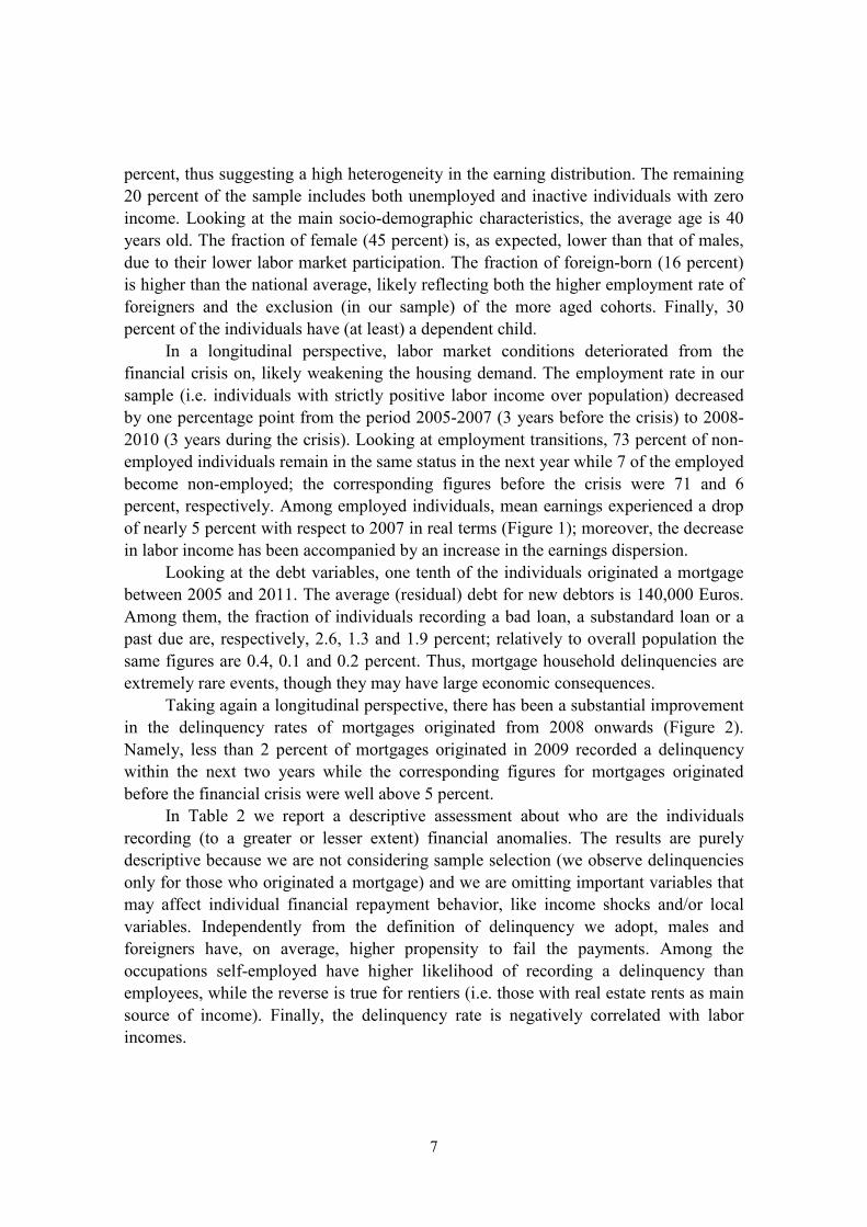
percent, thus suggesting a high heterogeneity in the earning distribution. The remaining 20 percent of the sample includes both unemployed and inactive individuals with zero income. Looking at the main socio-demographic characteristics, the average age is 40 years old. The fraction of female (45 percent) is, as expected, lower than that of males, due to their lower labor market participation. The fraction of foreign-born (16 percent) is higher than the national average, likely reflecting both the higher employment rate of foreigners and the exclusion (in our sample) of the more aged cohorts. Finally, 30 percent of the individuals have (at least) a dependent child.

In a longitudinal perspective, labor market conditions deteriorated from the financial crisis on, likely weakening the housing demand. The employment rate in our sample (i.e. individuals with strictly positive labor income over population) decreased by one percentage point from the period 2005-2007 (3 years before the crisis) to 2008-2010 (3 years during the crisis). Looking at employment transitions, 73 percent of non-employed individuals remain in the same status in the next year while 7 of the employed become non-employed; the corresponding figures before the crisis were 71 and 6 percent, respectively. Among employed individuals, mean earnings experienced a drop of nearly 5 percent with respect to 2007 in real terms (Figure 1); moreover, the decrease in labor income has been accompanied by an increase in the earnings dispersion.

Looking at the debt variables, one tenth of the individuals originated a mortgage between 2005 and 2011. The average (residual) debt for new debtors is 140,000 Euros. Among them, the fraction of individuals recording a bad loan, a substandard loan or a past due are, respectively, 2.6, 1.3 and 1.9 percent; relatively to overall population the same figures are 0.4, 0.1 and 0.2 percent. Thus, mortgage household delinquencies are extremely rare events, though they may have large economic consequences.

Taking again a longitudinal perspective, there has been a substantial improvement in the delinquency rates of mortgages originated from 2008 onwards (Figure 2). Namely, less than 2 percent of mortgages originated in 2009 recorded a delinquency within the next two years while the corresponding figures for mortgages originated before the financial crisis were well above 5 percent.

In Table 2 we report a descriptive assessment about who are the individuals recording (to a greater or lesser extent) financial anomalies. The results are purely descriptive because we are not considering sample selection (we observe delinquencies only for those who originated a mortgage) and we are omitting important variables that may affect individual financial repayment behavior, like income shocks and/or local variables. Independently from the definition of delinquency we adopt, males and foreigners have, on average, higher propensity to fail the payments. Among the occupations self-employed have higher likelihood of recording a delinquency than employees, while the reverse is true for rentiers (i.e. those with real estate rents as main source of income). Finally, the delinquency rate is negatively correlated with labor incomes.

7

The pool of borrowers has changed over the years both in quantity – as can be concluded by looking at the ratio between the number of new borrowers and the reference population – and in quality, as suggested by the predicted probability of recording a delinquency (based on the regression presented in Table 2). According to our data, new borrowers in the mortgage market were about 2 percent of the reference population between 2005 and 2007 and sharply decreased to around 1.5 percent in the subsequent three years (Figure 3a). As far the quality of new borrowers is concerned, they have, on average, a lower predicted probability of delinquency (Figure 3b), suggesting that debtors are positively selected with respect to the remainder of the population (e.g. they disproportionately belong to higher income classes). However, the relative quality of new borrowers changed over the years. Namely, after the 2008 crisis the predicted probability of delinquency for the whole population increased, while the same figure for the group of new borrowers progressively decreased.

In Figure 4 we examine the change in the selection of borrowers looking at the main socioeconomic characteristics. Borrowers’ labor income is higher compared to the rest of the population; however, this earning-gap increased from around 8,500 Euros in the period 2005-2007 to nearly 10,000 Euros in the period 2008-2010 (Figure 4a). Moreover, compared to the rest of the population, after the crisis new borrowers were older (Figure 4b) and with a slight prevalence of females (Figure 4c). Finally, the fraction of foreign-born among new borrowers decreased from 14.4 percent to 9.0 percent, widening the gap with respect to the corresponding figure in the rest of population (Figure 4d).

Many other variables, that are unobservable for the econometrician and observable for the local bank manager managing the loan approval process, may have affected selection. They may include additional sources of income not recorded in the tax declarations, the type of the job contract, the strength of the family ties (representing a source of monetary and non-monetary support to the borrower), the market value of the house and other soft information related to the borrower creditworthiness. In the next section we discuss how to address these issues with a more rigorous empirical framework.

3. The estimation strategy We examine how mortgage delinquencies react to income changes, conditional on

selection of individuals into indebtedness. To this end we rely on a standard Heckman approach that has been repeated for different cohorts of mortgages, thus directly assessing the time-varying selection.

3.1 Heckman selection models

Let 𝑖𝑖 be an individual who must choose on mortgage origination (𝑚𝑚) at time 𝑡𝑡 and, eventually, on subsequent delinquent behavior (𝑑𝑑) between time 𝑡𝑡 and time 𝑡𝑡 + 𝑘𝑘.

8

The propensity to originate a mortgage and to be delinquent (conditional on having originated a mortgage) can be represented by two latent variables:

𝑦𝑦𝑚𝑚,𝑖𝑖,𝑡𝑡∗ = 𝑥𝑥𝑖𝑖,𝑡𝑡𝛿𝛿 + 𝜀𝜀𝑚𝑚,𝑖𝑖,𝑡𝑡 (1)

𝑦𝑦𝑑𝑑,𝑖𝑖,𝑡𝑡+𝑘𝑘∗ = 𝑧𝑧𝑖𝑖,𝑡𝑡+𝑘𝑘𝛾𝛾 + 𝜀𝜀𝑑𝑑,𝑖𝑖,𝑡𝑡+𝑘𝑘 (2)

They are both expressed as the sum of an observed component (𝑥𝑥𝑖𝑖,𝑡𝑡 and 𝑧𝑧𝑖𝑖,𝑡𝑡+𝑘𝑘, respectively) and an unobserved random component (𝜀𝜀𝑚𝑚,𝑖𝑖,𝑡𝑡 and 𝜀𝜀𝑑𝑑,𝑖𝑖,𝑡𝑡+𝑘𝑘, respectively). Of course, individual propensities are unobservables. However, the origination of the mortgage is observable and can be defined as a binary outcome:

𝑦𝑦𝑚𝑚,𝑖𝑖,𝑡𝑡 = �10 𝑖𝑖𝑖𝑖 𝜀𝜀𝑚𝑚,𝑖𝑖,𝑡𝑡 > −𝑥𝑥𝑖𝑖,𝑡𝑡𝛿𝛿

𝑜𝑜𝑡𝑡ℎ𝑒𝑒𝑒𝑒𝑒𝑒𝑖𝑖𝑒𝑒𝑒𝑒 (3)

Subsequently, conditional on having got a mortgage, the repayment behavior can be defined as:

𝑦𝑦𝑑𝑑,𝑖𝑖,𝑡𝑡+𝑘𝑘 = �10 𝑖𝑖𝑖𝑖 𝜀𝜀𝑑𝑑,𝑖𝑖,𝑡𝑡+𝑘𝑘 > −𝑧𝑧𝑖𝑖,𝑡𝑡+𝑘𝑘𝛾𝛾

𝑜𝑜𝑡𝑡ℎ𝑒𝑒𝑒𝑒𝑒𝑒𝑖𝑖𝑒𝑒𝑒𝑒 (4)

Namely, 𝑦𝑦𝑑𝑑,𝑖𝑖,𝑡𝑡+𝑘𝑘 is observed only when 𝑦𝑦𝑚𝑚,𝑖𝑖,𝑡𝑡 = 1, i.e. for a non-random sample of the population. Moreover, we let 𝑦𝑦𝑑𝑑,𝑖𝑖,𝑡𝑡+𝑘𝑘 be equal to 1 if the credit status of individual 𝑖𝑖 records a deterioration within 2 years after mortgage origination and 0 otherwise. Deterioration means the switch from a status of performing loan to a delinquency (bad or substandard loans or past due). We also assume that the error components 𝜀𝜀𝑚𝑚,𝑖𝑖 and 𝜀𝜀𝑑𝑑,𝑖𝑖 are correlated across individuals and are drawn from a bivariate normal distribution with a correlation coefficient 𝜌𝜌.

Since different types of repayment delinquencies can be interpreted in terms of increasing degree of financial bad health, we also rely on an ordered probit with sample selection. The latter can be thought as an extension of the Heckman probit. Equation (4) is thus re-written as:

𝑦𝑦𝑑𝑑,𝑖𝑖,𝑡𝑡+𝑘𝑘 = 𝑗𝑗 𝑖𝑖𝑖𝑖 𝑐𝑐𝑗𝑗−1 < 𝑦𝑦𝑑𝑑,𝑖𝑖,𝑡𝑡+𝑘𝑘∗ < 𝑐𝑐𝑗𝑗 (5)

In words, the latent variable 𝑦𝑦𝑑𝑑,𝑖𝑖,𝑡𝑡+𝑘𝑘∗ is related to the outcome 𝑦𝑦𝑑𝑑,𝑖𝑖,𝑡𝑡+𝑘𝑘 through the

observational rule (5), where 𝑗𝑗 represents the hierarchically ordered alternative (i.e. performing loan, past due, substandard loan and bad loans) and 𝑐𝑐 is a set of strictly increasing thresholds that partition 𝑦𝑦𝑑𝑑,𝑖𝑖,𝑡𝑡+𝑘𝑘

∗ into 𝑗𝑗 exhaustive and mutually exclusive intervals. Selectivity effects are allowed to operate again through the correlation between the latent regression errors.

The set of variables 𝑧𝑧𝑖𝑖 includes controls for initial conditions (i.e. variables observed at the time of mortgage origination) and controls for changes in individual variables after mortgage origination. The set of variables 𝑥𝑥𝑖𝑖 includes the same variables observed at the time of mortgage origination included in 𝑧𝑧𝑖𝑖, and an exclusion restriction.

9

The latter is a variable affecting the probability to get a mortgage but which is unrelated to household repayment behavior in the subsequent years and it is necessary to identify the model.

Among the initial conditions observed at time t (i.e. variables that may affect both the probability of originating a mortgage at time t and the ability to repay it later) we include the log of after-tax labor income, the log of income from rents (a proxy also for individual wealth), dummies for the occupational status (identified with the main source of income), age and age squared, dummies for gender, country of birth (i.e. natives and foreign-born) and the presence of dependent children. The set of initial conditions includes also local level variables, such as the log of house price in the city where the individual resides, the employment rate and the population density at the time of mortgage origination. Finally, dummies for geographical areas capture other unobserved local variables.

In the main equation, i.e. the probability of being delinquent within two years, we also include variables capturing changes occurred after mortgage origination such house price change (that may affect the propensity to repay the debt) and labor income changes (that may affect the capability to repay the debt). Specifically, the labor income change is measured as (𝑦𝑦𝑡𝑡+2 − 𝑦𝑦𝑡𝑡) (0.5 ∙ 𝑦𝑦𝑡𝑡+2 + 0.5 ∙ 𝑦𝑦𝑡𝑡)⁄ . The variable varies within the interval [−2; 2] and captures changes occurred with respect to the mortgage origination year; extreme values −2 and 2 capture transitions from employment to non-employment status occurred within this time interval and vice versa (i.e. a change from positive/zero labor income to zero/positive labor income).10

3.2 The exclusion restriction

Our exclusion restriction is a quantitative index of credit supply at the local level, aimed at capturing the orientation of bank lending policies in the local credit market where the individual lives. In order to identify the credit supply orientation at the local level, we proceed in two steps.

First we run the regression:

𝑚𝑚𝑏𝑏,𝑝𝑝,𝑡𝑡 = 𝜋𝜋𝑝𝑝×𝑡𝑡 + 𝜋𝜋𝑏𝑏×𝑡𝑡 + 𝜇𝜇𝑏𝑏,𝑝𝑝,𝑡𝑡 (6)

where the dependent variable is the log of mortgages by bank 𝑏𝑏 in province 𝑝𝑝 at time 𝑡𝑡. The set of dummies 𝜋𝜋𝑝𝑝×𝑡𝑡 is defined for each province-year and captures any variable varying at the province-year level (e.g. local economic cycle). The variable 𝜋𝜋𝑏𝑏×𝑡𝑡 is a set of dummies for bank-year measuring the time-varying bank lending policy. This is a pure supply factor since the aggregate mortgage demand is controlled with the province-

10 A virtue of this measure is that it facilitates an integrated treatment of transitions from employment to unemployment and changes in income for those who continue to be employed. Moreover, this variable is related to the conventional income growth rate measure (the two measures are approximately equal for small growth rates), while delivering a variable with a much smoother distribution.

10

year fixed effects. Last, 𝜇𝜇𝑏𝑏,𝑝𝑝,𝑡𝑡 is the error term. Regression (6) has been run on a different dataset, drawn from the Bank of Italy, and referring to the universe of bank loans to the household sector.11 The identification of 𝜋𝜋𝑏𝑏×𝑡𝑡 is guaranteed by the presence of multiple banks in each province (i.e. multiple banks exposed to the same local demand) and the presence of each bank in multiple provinces (i.e. multiple provinces exposed to the same bank’s supply condition).

The bank-year 𝜋𝜋𝑏𝑏×𝑡𝑡 variable is the main input for the construction of the credit supply index used as exclusion restriction. To check the goodness of our bank-year indicator we have first examined its correlation with the “diffusion index” provided by the Bank Lending Survey of ECB (BLS), which collects qualitative information on Euro area main credit supply, by the mean of a questionnaire to the largest banks, and it is used to construct various indexes of banks’ lending policies.12 The correlation between the latter and 𝜋𝜋𝑏𝑏×𝑡𝑡 for the largest Italian banks estimated through equation (6) is reported in Figure 5. As expected the two lines mirror each other. Indeed, positive values of the diffusion index suggest a tightening of credit standards applied to loan approval decisions and lower values of 𝜋𝜋𝑏𝑏×𝑡𝑡 indicate less expansive lending policy of the banks.

In Table 3 we perform a statistical test for the predictive power of our bank-year credit supply indicator. Namely, we consider the period 2005-2010 and we regress the log of loans of each bank to the household sector on 𝜋𝜋𝑏𝑏×𝑡𝑡; the specification also includes bank fixed effects, to capture time-invariant factors that characterize each bank, and year dummies, to capture trend common to all banks. The credit supply indicator enters with the positive sign, as expected, and is highly significant. The impact is also substantial from an economic point of view since one standard deviation in the bank-year indicator leads to an increase of nearly half the standard deviation in the log of loans.

Second, since our aim is to get an index of credit supply at the local level, under the assumption that the individual probability to get a mortgage is affected by the credit policy of banks located in the place he/she lives, the bank-year dummies 𝜋𝜋𝑏𝑏×𝑡𝑡 are aggregated at the local level using, as weights, the number of branches of each bank in the local labor market (LLM, since, differently from data on loans we have data on branches with this higher level of detail13) at time 𝑡𝑡 − 1. Formally:

11 More precisely, the data are drawn from the Bank of Italy Supervisory Report database, collecting data on the balance sheets (including loans) of all banks operating in Italy. 12 The diffusion index is the (weighted) difference between the share of banks reporting that credit standards have been tightened and the share of banks reporting that they have been eased. See e.g. http://www.ecb.europa.eu/stats/money/surveys/lend/html/index.en.html 13 LLM is a geographic unit represented by cluster of municipalities and built on the basis of intra-municipality daily commuting patterns. LLMs in Italy are more numerous than provinces and they are arguably closer to the definition of local credit market. However, since we do not have data on loans by LLM we cannot estimate equation 3 at the level of LLM.

11

𝐶𝐶𝐶𝐶𝑙𝑙,𝑡𝑡 = �𝑏𝑏𝑒𝑒𝑏𝑏𝑏𝑏𝑐𝑐ℎ𝑒𝑒𝑒𝑒𝑏𝑏,𝑙𝑙,𝑡𝑡−1

𝑏𝑏𝑒𝑒𝑏𝑏𝑏𝑏𝑐𝑐ℎ𝑒𝑒𝑒𝑒𝑙𝑙,𝑡𝑡−1𝑏𝑏∙ 𝜋𝜋𝑏𝑏×𝑡𝑡 (7)

where 𝐶𝐶𝐶𝐶𝑙𝑙,𝑡𝑡 captures the orientation of the credit supply in the local credit market 𝑙𝑙 at time 𝑡𝑡 and it is expected to be positively related to the likelihood of originating a mortgage in the same local credit market at the same year (i.e. intention to treat). The sources of variability are the substantial heterogeneity in lending policies across banks and the variation of banks’ market share at the local level.

An implicit assumption of the exclusion restriction is that the banks’ nationwide lending policies (𝜋𝜋𝑏𝑏×𝑡𝑡) are unaffected by unobserved factors at the local level. This assumption might be violated when some province markets are relevant for banks’ lending policies. This may happen both when the province is large with respect to the national credit market or when the bank’s credit market is very concentrated in a given territory (e.g. in the case of small banks). Moreover, some banks might systematically sort into specific provinces anticipating local future prospects. These violations of our assumption would undermine the validity of the research design. In order to address these issues and to reinforce the exogeneity of the indicator, the bank fixed effects used to build the aggregate indicator for the LLM l belonging to province p are estimated on a regression sample including all provinces but p. This strategy allows avoiding that unobservable shocks in province p affect the lending policies of banks operating in that province.

Figure 6 reports the distribution of credit supply index across LLMs and over time. There is a remarkable heterogeneity of the index at the local level: the ratio between the interquartile range and the median is about 70 percent. Moreover, from the financial crisis onwards there was a shift towards left of the distribution of the index, suggesting a tightening of the credit supply conditions at the local level. Unsurprisingly, the local credit supply explains a significant fraction of the reduction in the entry into the mortgage market between the years before and after the financial crisis. Table 4 displays the Oaxaca-Blinder decomposition of this difference. According to our estimates, individual variables explain about 20 percent of the reduction in the entry rate (column I). The explained fraction of the gap increases only marginally when adding local variables (column II) and significantly when adding 𝐶𝐶𝐶𝐶𝑙𝑙,𝑡𝑡 (column III). Local lending policies, as captured by our proxy, account for roughly one third of the explained gap. Since this index is unrelated by construction to current local conditions, it provides an exogenous source of variation for the probability to get a mortgage, randomizing selection into indebtedness.

12

4. Results

4.1 Main findings

We consider different cohorts of mortgages. For each cohort, we first model the selection process driving the decision to become indebted, including standard personal characteristics and the credit-supply index described in Section 3. Second, we focus on income changes, i.e. changes occurred after the mortgage origination, and their association with the probability of default. The two steps are estimated simultaneously by maximum likelihood using a standard Heckman probit model. However, for sake of clarity, we comment the two steps separately.

In Table 5 we report the marginal effects of the probit in the selection equation. We consider cohorts of mortgages from 2005 to 2009 because, as our dataset is limited to 2011, these are the only ones we re-observe after two years from mortgage origination. Income is positively correlated with the probability of becoming indebted, suggesting that, on-average, indebted people are richer than the rest of the population. The credit supply indicator 𝐶𝐶𝐶𝐶𝑙𝑙,𝑡𝑡 enters, as expected, with a positive effect and it is highly significant in all years, even if in 2008 and 2009 its marginal impact declined, probably due to the banks’ lower propensity towards lending.

In Tables 6 we report the marginal effects of the main equation, where the dependent variable is a wide definition of financial bad health, which includes bad loans, substandard loans and past due.14 Moreover, the table reports two different estimates for each cohort, the first being from a simple probit on the selected sample of borrowers and the second from the Heckman probit, thus taking into account the selection process into the mortgage market.

Consider first the coefficient of the selectivity term 𝜆𝜆, which is always negative, but it is significantly different from zero only for the two more recent cohorts (2008 and 2009). Moreover, also the absolute value of the coefficient increases, reaching its peak, again, for more recent cohorts of mortgages. The sign and the magnitude of the impact of 𝜆𝜆 depend on the parameter 𝜌𝜌 that captures the correlation between 𝜀𝜀𝑖𝑖 and 𝜇𝜇𝑖𝑖. Therefore there are unobserved (to the econometrician) factors positively affecting mortgage origination and negatively correlated with the probability of observing financial difficulties (or vice versa). This evidence, as expected, signals positive selection of the borrowers on unobservables. Moreover, the relevance of those factors was negligible (both economically and statistically) before the financial crisis and

14 The wide definition is our preferred indicator. Indeed, the latter indicates with certainty the existence of a financial difficulty, while the same is not true for substandard and bad loans that are affected, to some extent, by a subjective evaluation of the lender. For instance, the transition from past due to bad loan can be delayed by internal organizational procedures or because the lender voluntarily allowing the lengthening of the delinquency period. In other words, while the existence of an anomaly unambiguously identifies a financial difficulty, the degrees of anomaly depend also on some external factors that may have little to do with it.

13

sizeable after the crisis. According to our estimates (i.e. multiplying the average Inverse Mill’s ratio by its marginal effect at the average), the selection process in mortgage origination reduced the probability of default by around 50 percent in the period 2008-2009, which corresponds to a 3.5 points decrease in the delinquency rate. Before the crisis the corresponding figures, though not statistically significant, were much lower in magnitudes (less than 10 per cent and 0.3 points, respectively).

As far as labor income changes are concerned, the parameter of interest varies between 0.2 and 0.3. Therefore, a 10 percent negative income change leads to an increase between 0.2 and 0.3 percentage points in the probability of delinquency, which roughly corresponds to a 5 percent increase in the observed delinquency rate. In case of job loss (which, according to our variable, corresponds to a -200 percent decrease in earnings) the delinquency rate nearly doubles. Also initial conditions matter. Having an income 10 percent higher at the mortgage origination reduces the delinquency rate by around 0.1-0.2 percentage points.

The correction for sample selection, with respect to the simple probit model, leads to larger negative effect for both income variation and income at origination. The size of the bias for the two more recent cohorts is between 30 and 40 percent of the true parameter. Therefore, unobserved factors are positively related to income and their omission may severely bias the estimates.

4.2 Robustness

To check the robustness of our findings we enrich the previous specifications along several directions.

In Table 7, we use the same set of variables in both the selection and the main equation (with the exception of the exclusion restriction). Indeed, income and/or house price changes after mortgage origination can be partly anticipated (at the time of mortgage origination) and, therefore, they may affect selection into indebtedness. According to our findings, income changes are positively correlated with the probability of originating a mortgage. However, and more importantly, the key findings on the role of selection and on the sensitivity of the delinquency rate to income shock are unchanged.

In Table 8, we enrich the specification with further controls. Namely, we add two individual-level variables: the log of the debt and a dummy for debts that are jointly held by at least two individuals. Both variables are observed, by definition, only for individuals with a debt and, therefore, may be included only in the main equation. They are plausibly correlated with individual riskiness and, therefore, may capture factors affecting both the probability of recording a delinquency and the probability to get a mortgage. Moreover, we add a variable capturing changes in the delinquency rate at the bank level. Indeed one may argue that easier credit conditions at time t may affect future banks’ propensity to report and address household financial difficulties and, consequently, the individual probability of default. Finally, we add local-level variables

14

that are aimed at capturing unobserved features of the local financial development. The first is the density of bank branches (i.e. branches per square meter), used as a proxy for the accessibility of the banking system. The second is the Herfindahl index, which proxies the degree of banking competition at the local level. Both variables may be correlated to both the probability of originating a mortgage and of recording a delinquency and are included in both the selection and the main equation. We find that higher debts increase financial vulnerability while joints debts reduce it; among the other variables, higher bank concentration and lower branch density reduce the probability of mortgage origination though they are substantially unrelated to individual delinquency rate. As far our key variables, the selectivity term continues to be significant (and with the expected sign) only for the more recent cohorts and the coefficients of explanatory variables in the main equation are qualitatively similar to those of our baseline specification.

Our main estimates, as already mentioned, refer to all loans larger than 75,000 Euros, independently from the motivation of the loan. They may also include loans of self-employed people to finance their activities. Moreover, income from self-employment is severely underreported in tax records (Marino and Zizza, 2011). To control for this sources of heterogeneity and mis-measurement, which could affect the analysis of both the selection process and the repayment behavior, in Table 9 we replicate our estimates in a sub-sample which excludes self-employed. The sign and the size of the estimated coefficients are again qualitatively similar.

Finally, in Table 10 we adopt a different empirical strategy, relying to an ordered probit with selection correction. We exploit the fact that the performing status of loans can be hierarchically ordered, going from the status of (1) performing loan to, in increasing order of financial bad health, (2) past due, (3) substandard loan and (4) bad loan (see also equation 5). The results should be interpreted with caution since the attribution to a certain financial status partly depends on idiosyncratic bank features. However, our key findings are qualitatively similar to those discussed above.

5. Conclusions Why some indebt individuals stop repaying debt? In institutional settings where

there is limited room for strategic behavior and the consequences of being registered as delinquent are severe, other factors may play a relevant role.

On this respect, our paper sheds light on two important and almost neglected issues: selection into the mortgage market and income changes after mortgage origination. According to our findings, the impact of labor market income changes is sizeable, as an episode of unemployment more than doubles the individual delinquency rate. Second, the tightening of the selection process from the Global Financial Crisis on largely explains the trend in delinquency rates of the most recent cohorts of mortgages. Neglecting selection mechanisms may severely bias the estimates of individuals’ credit risk.

15

The huge impact of selection and job loss we found in a country like Italy, traditionally characterized by prudent lending policies and strong employment protection for permanent workers calls for further scrutiny of these channels also in other countries, where both employment protection and lending policies are less tight. Our results also suggest that instruments designed to absorb the consequences of income shocks, like for instance the unemployment benefit, tax cuts and in general any policy which relaxes household financial constraints, may have positive effects not only on household consumption, but also on financial stability as they reduce the probability of default. Finally, our results suggest that credit risk models as those typically used by lenders, may systematically underestimate the relationship between income and the probability of default: this may lead to loan mispricing and sub-optimal risk composition of the borrowers.

16

References Acciari, P., E. Manzoli, S. Mocetti and E. Viviano (2014), La vulnerabilità

finanziaria: un’analisi per classi di reddito, Moneta e Credito, 67: 401-428. Aiyar, S. (2012), From financial crisis to Great Recession: the role of globalized

banks, American Economic Review: Papers & Proceedings, 102: 225-230. Adams, W., L. Einav and J. Levin (2009), Liquidity constraints and imperfect

information in subprime lending, American Economic Review 99: 49-84. Bajari, P., S. Chu, D. Nekipelov and M. Park (2013), A dynamic model of

subprime mortgage default: estimation and policy implications, NBER working paper 18850.

Boheim, R. and M.P. Taylor (2000), My home was my castle: evictions and repossessions in Britain, Journal of Housing Economics, 9: 287-319.

Boyes, W.J., D.L. Hoffman and S.A. Low (1989), An econometric analysis of the bank credit scoring problem, Journal of Econometrics, 40: 3-14.

Deng, Y., J.M. Quigley and R. van Order (2000), Mortgage terminations, heterogeneity, and the exercise of mortgage options, Econometrica, 68: 275-307.

Demyanyk, Y. and O. van Hemert (2011), Understanding the subprime mortgage crisis, Review of Financial Studies, 24: 1847-1880.

Diaz-Serrano, L. (2005), Income volatility and residential mortgage delinquency across the EU, Journal of Housing Economics, 14: 153-177.

Domowitz I. and R.L. Sartain (1999), Determinants of the consumer bankruptcy decision, Journal of Finance, 44:403-420.

Duygan-Bump, B. and C. Grant (2009), Household debt repayment behavior: what role do institutions play? Economic Policy, 24: 107-140.

Fay, S., E. Hurst and M.J. White (2002), The household bankruptcy decision, American Economic Review, 92: 706-718.

Foote, C., K. Gerardi and P. Willen (2008), Negative equity and foreclosure: theory and evidence, Journal of Urban Economics, 64: 234-245.

Gathergood, J. (2009), Income shocks, mortgage repayment risk and financial distress among UK households, working paper.

Gerardi, K., K.F. Herkenhoff, L.E. Ohanian and P.S. Willen (2013), Unemployment, negative equity, and strategic default, working paper.

Greenstone, M., A. Mas and H.L. Nguyen (2014), Do credit market shocks affect the real economy? Quasi-experimental evidence from the Great Recession and ‘normal’ economic times, NBER working paper 20714.

17

Gross, D.B. and N.S. Souleles (2002), An empirical analysis of personal bankruptcy and delinquency, Review of Financial Studies, 15: 319-347.

Guiso, L., P. Sapienza and L. Zingales (2013), The determinants of attitudes towards strategic default on mortgages, Journal of Finance, 68: 1473-1515.

Haughwout, A., R. Peach and J. Tracy (2008), Juvenile delinquent mortgages: Bad credit or bad economy? Journal of Urban Economics, 64: 246-257.

Jacobson, T. and K. Roszbach (2003), Bank lending policy, credit scoring and value-at-risk, Journal of Banking and Finance, 27: 615-633.

Marino, M.R. and R. Zizza (2011), The personal income tax evasion in Italy: an estimate by taxpayer’s type, in M. Pickhardt and A. Prinz (eds.), Tax evasion and the shadow economy, Edward Elgar Publishing.

Mayer, C., K. Pence and S.M. Sherlund (2009), The rise in mortgage defaults, Journal of Economic Perspectives, 23: 27-50.

Mian, A. and A. Sufi (2009), The consequences of mortgage credit expansion: evidence from the U.S. mortgage default crisis, Quarterly Journal of Economics, 124: 1449-1496.

18

Figures

Figure 1. Income trend

We consider only individual with strictly positive labor income and in the age-bracket 25-54. Source: authors’ elaborations on data from TR and CR.

Figure 2. Mortgage delinquency rate

Delinquency rates for different cohorts of mortgages (years in the x-axis refer to origination). Source: authors’ elaboration on data from CR.

0

1

2

3

4

5

6

2005 2006 2007 2008 2009

% bad or substandard loans or past due(2 years after origination)

19

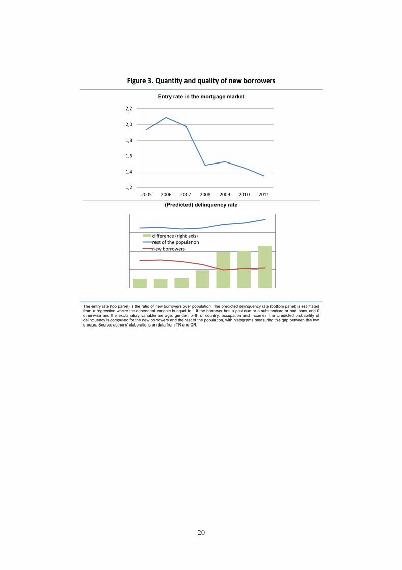
Figure 3. Quantity and quality of new borrowers

Entry rate in the mortgage market

(Predicted) delinquency rate

The entry rate (top panel) is the ratio of new borrowers over population. The predicted delinquency rate (bottom panel) is estimated from a regression where the dependent variable is equal to 1 if the borrower has a past due or a substandard or bad loans and 0 otherwise and the explanatory variable are age, gender, birth of country, occupation and incomes; the predicted probability of delinquency is computed for the new borrowers and the rest of the population, with histograms measuring the gap between the two groups. Source: authors’ elaborations on data from TR and CR.

1,2

1,4

1,6

1,8

2,0

2,2

2005 2006 2007 2008 2009 2010 2011

20

Figure 4. Positive selection of new borrowers before and after the crisis

The histograms represent the difference in the observables between the new borrowers and the rest of the population; for each observable differences are computed for the years before and after the crisis.

Figure 5. BLS and the credit supply index

The blue line represents credit supply conditions as measured by the BLS (yearly values from Figure 4); positive (negative) values indicate a tightening (easing) of credit conditions. The red line is the credit supply index for the largest Italian banks as estimated from equation (6); higher (lower) values indicate more (less) expansive lending policies. Source: authors’ elaboration on data drawn from Bank of Italy.

7000

8000

9000

10000

2005-2007 2008-2010

differences in earningsnew borrowers vs. rest of the population

-3,0

-2,0

-1,0

0,0

2005-2007 2008-2010

differences in agenew borrowers vs. rest of the population

-2,0

-1,0

0,0

1,0

2,0

2005-2007 2008-2010

differences in the fraction of femalesnew borrowers vs. rest of the population

-8,0

-6,0

-4,0

-2,0

0,0

2005-2007 2008-2010

differences in the fraction of foreign-bornnew borrowers vs. rest of the population

1,90

2,00

2,10

2,20

2,30

-0,10

0,00

0,10

0,20

0,30

2005 2006 2007 2008 2009

BLS (left axis)

CS (right axis)

21

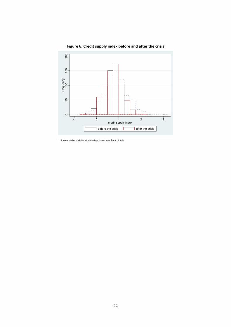
Figure 6. Credit supply index before and after the crisis

Source: authors’ elaboration on data drawn from Bank of Italy.

22

Tables

Table 1. Descriptive statistics Mean St. dev. 25° 75°

Individual variables:

% of individual with positive income 80.0 40.0 1 1 Income (thousands of Euros) 17.3 23.4 9.2 21.5 % of employees 75.1 43.2 1 1

Age 40.0 10.2 32 48 % female 44.7 49.7 0 1 % foreign-born 16.3 36.9 0 1 % dependent children 31.6 46.5 0 1 % of individuals who originate a mortgage 10.6 30.8 0 0

Debt (thousands of Euros) 140.5 120.7 95.8 156.7 % bad loans (new mortgages) 2.6 15.9 0 0 % substandard loans (new mortgages) 1.3 11.3 0 0 % past dues (new mortgages) 1.8 13.3 0 0

Local variables:

Credit supply 0.9 0.4 0.7 1.2 House price (Euros per sq. m.) 1,683 976 1,019 1,976 Employment rate 45.7 7.3 39.4 51.5 Population density 1.3 1.9 0.2 1.7 Source: Individual variables are drawn from TR and CR; local variables are drawn from Bank of Italy (the credit supply indicator), OMI (house prices) and Istat (employment rate and population density).

Table 2. Individual correlates of mortgage delinquency Dependent variable: Delinquency Female -0.285*** (0.006) Age 0.012*** (0.004) Age squared 0.014*** (0.005) Dependent children 0.019*** (0.006) Foreign-born 0.367*** (0.007) Log of labor income -0.188*** (0.005) Log of income from rents -0.083*** (0.001) Main source of incomes: Pensions -1.225*** (0.058) Self-employment 0.104*** (0.008) Rents -1.200*** (0.050) Observations 611,121 The table reports the marginal effects of a cross-section where the dependent variable is the existence of a debt delinquency; the sample includes individuals who originate a debt, independently from when it was originated; robust standard errors in parentheses; *, **, *** mean significantly different from zero at the 10, 5 and 1 percent level, respectively.

23

Table 3. Credit and supply conditions Dependent variable: Log of loans to the households Credit supply index 0.843*** (0.010) Year FE YES Bank FE YES Observations 3,372 R-squared 0.813 The table reports the estimates of a panel where the dependent variable is the log of the loans to the household sector of bank b in the year t (period 2005-2010) and the key explanatory variable is 𝜋𝜋𝑏𝑏×𝑡𝑡 estimated in equation (6); robust standard errors in parentheses; *, **, *** mean significantly different from zero at the 10, 5 and 1 percent level, respectively.

Table 4. Entry rate before and after the crisis

Specification: I II III Individual controls YES YES YES Local controls - YES YES 𝐶𝐶𝐶𝐶𝑙𝑙,𝑡𝑡 - - YES Entry rate in the period 2005-2007 1,830 1,830 1,830 Entry rate in the period 2008-2010 1,380 1,380 1,380 Difference (a) 0,450 0,450 0,450 Explained by covariates (b) 0,071 0,076 0,118 % explained by covariates (b)/(a) 15.8 16.9 26.2 The table reports the Oaxaca-Blinder decomposition of the difference in the entry rate between the periods before and after the financial crisis; individual controls include age, gender, dependent children, country of birth, log of incomes and occupational dummies, local controls include log of house prices, employment rate, population density and geographical dummies.

24

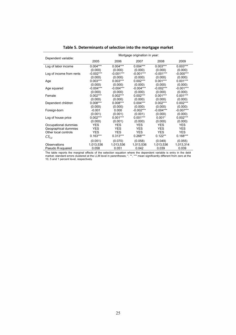
Table 5. Determinants of selection into the mortgage market

Dependent variable: Mortgage origination in year:

2005 2006 2007 2008 2009 Log of labor income 0.004*** 0.004*** 0.004*** 0.003*** 0.003*** (0.000) (0.000) (0.000) (0.000) (0.000) Log of income from rents -0.002*** -0.001*** -0.001*** -0.001*** -0.000*** (0.000) (0.000) (0.000) (0.000) (0.000) Age 0.003*** 0.003*** 0.002*** 0.001*** 0.001*** (0.000) (0.000) (0.000) (0.000) (0.000) Age squared -0.004*** -0.004*** -0.004*** -0.002*** -0.001*** (0.000) (0.000) (0.000) (0.000) (0.000) Female 0.002*** 0.002*** 0.002*** 0.001*** 0.001*** (0.000) (0.000) (0.000) (0.000) (0.000) Dependent children 0.008*** 0.008*** 0.004*** 0.002*** 0.002*** (0.000) (0.000) (0.000) (0.000) (0.000) Foreign-born -0.001 0.000 -0.002*** -0.004*** -0.007*** (0.001) (0.001) (0.001) (0.000) (0.000) Log of house price 0.002*** 0.001*** 0.001*** 0.001* 0.002*** (0.000) (0.001) (0.000) (0.000) (0.000) Occupational dummies YES YES YES YES YES Geographical dummies YES YES YES YES YES Other local controls YES YES YES YES YES 𝐶𝐶𝐶𝐶𝑙𝑙,𝑡𝑡 0.163*** 0.313*** 0.268*** 0.122** 0.168*** (0.051) (0.070) (0.058) (0.049) (0.055) Observations 1,013,536 1,013,536 1,013,536 1,013,536 1,013,314 Pseudo R-squared 0.058 0.051 0.042 0.039 0.039 The table reports the marginal effects of the selection equation where the dependent variable is entry in the debt market; standard errors clustered at the LLM level in parentheses; *, **, *** mean significantly different from zero at the 10, 5 and 1 percent level, respectively.

25

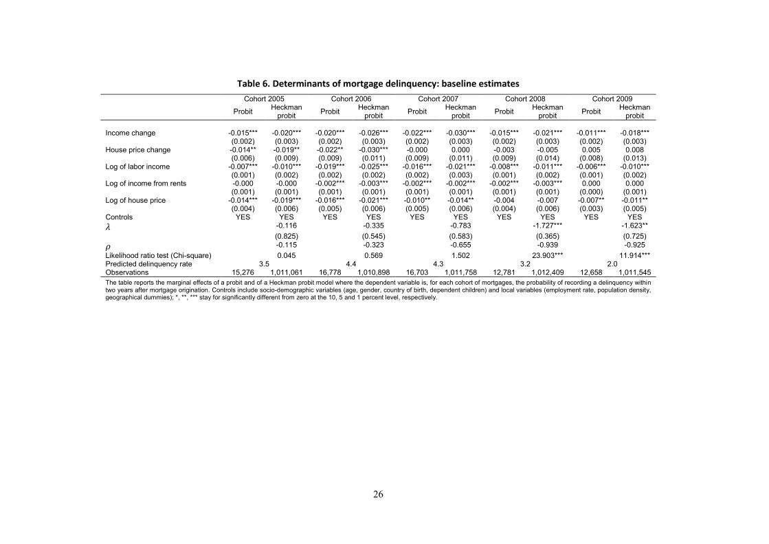
Table 6. Determinants of mortgage delinquency: baseline estimates Cohort 2005 Cohort 2006 Cohort 2007 Cohort 2008 Cohort 2009 Probit Heckman

probit Probit Heckman probit Probit Heckman

probit Probit Heckman probit Probit Heckman

probit Income change -0.015*** -0.020*** -0.020*** -0.026*** -0.022*** -0.030*** -0.015*** -0.021*** -0.011*** -0.018*** (0.002) (0.003) (0.002) (0.003) (0.002) (0.003) (0.002) (0.003) (0.002) (0.003) House price change -0.014** -0.019** -0.022** -0.030*** -0.000 0.000 -0.003 -0.005 0.005 0.008 (0.006) (0.009) (0.009) (0.011) (0.009) (0.011) (0.009) (0.014) (0.008) (0.013) Log of labor income -0.007*** -0.010*** -0.019*** -0.025*** -0.016*** -0.021*** -0.008*** -0.011*** -0.006*** -0.010*** (0.001) (0.002) (0.002) (0.002) (0.002) (0.003) (0.001) (0.002) (0.001) (0.002) Log of income from rents -0.000 -0.000 -0.002*** -0.003*** -0.002*** -0.002*** -0.002*** -0.003*** 0.000 0.000 (0.001) (0.001) (0.001) (0.001) (0.001) (0.001) (0.001) (0.001) (0.000) (0.001) Log of house price -0.014*** -0.019*** -0.016*** -0.021*** -0.010** -0.014** -0.004 -0.007 -0.007** -0.011** (0.004) (0.006) (0.005) (0.006) (0.005) (0.006) (0.004) (0.006) (0.003) (0.005) Controls YES YES YES YES YES YES YES YES YES YES 𝜆𝜆 -0.116 -0.335 -0.783 -1.727*** -1.623** (0.825) (0.545) (0.583) (0.365) (0.725) 𝜌𝜌 -0.115 -0.323 -0.655 -0.939 -0.925 Likelihood ratio test (Chi-square) 0.045 0.569 1.502 23.903*** 11.914*** Predicted delinquency rate 3.5 4.4 4.3 3.2 2.0 Observations 15,276 1,011,061 16,778 1,010,898 16,703 1,011,758 12,781 1,012,409 12,658 1,011,545 The table reports the marginal effects of a probit and of a Heckman probit model where the dependent variable is, for each cohort of mortgages, the probability of recording a delinquency within two years after mortgage origination. Controls include socio-demographic variables (age, gender, country of birth, dependent children) and local variables (employment rate, population density, geographical dummies); *, **, *** stay for significantly different from zero at the 10, 5 and 1 percent level, respectively.

26

Table 7. Determinants of mortgage delinquency: balanced equations Cohort 2005 Cohort 2006 Cohort 2007 Cohort 2008 Cohort 2009 Heckman

probit Heckman

probit Heckman

probit Heckman

probit Heckman

probit Income change -0.020*** -0.026*** -0.030*** -0.021*** -0.018*** (0.003) (0.003) (0.003) (0.003) (0.003) House price change -0.019** -0.030*** -0.000 -0.005 0.008 (0.009) (0.011) (0.011) (0.014) (0.013) Log of labor income -0.010*** -0.025*** -0.021*** -0.011*** -0.010*** (0.002) (0.002) (0.003) (0.002) (0.002) Log of income from rents -0.000 -0.003*** -0.002*** -0.003*** 0.000 (0.001) (0.001) (0.001) (0.001) (0.001) Log of house price -0.019*** -0.021*** -0.014** -0.007 -0.012** (0.006) (0.006) (0.006) (0.006) (0.005) Controls YES YES YES YES YES 𝜆𝜆 -0.214 -0.350 -0.816 -1.763** -1.637** (0.830) (0.540) (0.550) (0.787) (0.688) 𝜌𝜌 -0.211 -0.337 -0.673 -0.943 -0.927 Observations 1,011,061 1,010,898 1,011,758 1,012,409 1,011,545 The table reports the marginal effects of a Heckman probit model where the dependent variable is, for each cohort of mortgages, the probability of recording a delinquency within two years after mortgage origination. Controls include socio-demographic variables (age, gender, country of birth, dependent children) and local variables (employment rate, population density, geographical dummies); *, **, *** stay for significantly different from zero at the 10, 5 and 1 percent level, respectively.

Table 8. Determinants of mortgage delinquency: adding controls Cohort 2005 Cohort 2006 Cohort 2007 Cohort 2008 Cohort 2009 Heckman

probit Heckman

probit Heckman

probit Heckman

probit Heckman

probit Income change -0.015*** -0.019*** -0.020*** -0.018*** -0.018*** (0.002) (0.002) (0.002) (0.003) (0.003) House price change -0.017*** -0.026*** -0.003 -0.007 0.001 (0.006) (0.008) (0.008) (0.012) (0.012) Log of labor income -0.008*** -0.021*** -0.016*** -0.010*** -0.011*** (0.002) (0.002) (0.002) (0.002) (0.002) Log of income from rents -0.001 -0.003*** -0.002*** -0.003*** 0.000 (0.001) (0.001) (0.001) (0.001) (0.001) Log of house price -0.018*** -0.020*** -0.016*** -0.008 -0.013** (0.004) (0.005) (0.004) (0.005) (0.005) Log of debt 0.022*** 0.031*** 0.034*** 0.018*** 0.004 (0.003) (0.003) (0.003) (0.004) (0.004) Joint debt -0.010*** -0.025*** -0.021*** -0.021*** -0.029*** (0.003) (0.003) (0.003) (0.004) (0.004) Bank delinquency rate 0.001 0.001 0.007*** 0.001 0.002 (0.001) (0.001) (0.001) (0.002) (0.001) Bank branch density 0.001 0.000 0.002 -0.007 0.007 (0.005) (0.005) (0.005) (0.006) (0.006) Herfindahl index 0.008 -0.016 -0.011 -0.091 0.071** (0.047) (0.046) (0.044) (0.060) (0.035) Controls YES YES YES YES YES 𝜆𝜆 -0.474 -0.467 -0.620 -1.762*** -1.581*** (0.933) (0.667) (0.573) (0.659) (0.564) 𝜌𝜌 -0.441 -0.436 -0.551 -0.943 -0.919 Observations 1,011,058 1,010,898 1,011,755 1,012,407 1,011,536 The table reports the marginal effects of a Heckman probit model where the dependent variable is, for each cohort of mortgages, the probability of recording a delinquency within two years after mortgage origination. Controls include socio-demographic variables (age, gender, country of birth, dependent children) and local variables (employment rate, population density, geographical dummies); *, **, *** stay for significantly different from zero at the 10, 5 and 1 percent level, respectively.

27

Table 9. Determinants of mortgage delinquency: excluding self-employed individuals Cohort 2005 Cohort 2006 Cohort 2007 Cohort 2008 Cohort 2009 Heckman

probit Heckman

probit Heckman

probit Heckman

probit Heckman

probit Income change -0.013*** -0.016*** -0.018*** -0.016*** -0.012*** (0.002) (0.002) (0.002) (0.003) (0.003) House price change -0.017** -0.022*** -0.002 -0.008 0.009 (0.007) (0.009) (0.008) (0.012) (0.012) Log of labor income -0.008*** -0.019*** -0.016*** -0.009*** -0.009*** (0.002) (0.002) (0.002) (0.002) (0.002) Log of income from rents -0.000 -0.003*** -0.002** -0.004*** 0.000 (0.001) (0.001) (0.001) (0.001) (0.001) Log of house price -0.017*** -0.023*** -0.014*** -0.010* -0.013** (0.005) (0.005) (0.005) (0.006) (0.005) Controls YES YES YES YES YES 𝜆𝜆 -0.733 -0.206 -0.673 -1.589*** -1.595** (0.730) (0.809) (0.563) (0.537) (0.767) 𝜌𝜌 -0.625 -0.203 -0.587 -0.920 -0.921 Observations 891,012 887,008 885,788 897,251 900,696 The table reports the marginal effects of a Heckman probit model where the dependent variable is, for each cohort of mortgages, the probability of recording a delinquency within two years after mortgage origination. Controls include socio-demographic variables (age, gender, country of birth, dependent children) local variables (employment rate, population density, geographical dummies) and additional controls introduced in the previous robustness checks (log of debt, joint debt, bank delinquency rate, local branch density, herfindahl index); *, **, *** stay for significantly different from zero at the 10, 5 and 1 percent level, respectively.

Table 10. Determinants of mortgage delinquency: ordered probit

Cohort 2005 Cohort 2006 Cohort 2007 Cohort 2008 Cohort 2009 Income change -0.194*** -0.211*** -0.194*** -0.097*** -0.103** (0.058) (0.029) (0.057) (0.035) (0.043) House price change -0.181** -0.244*** 0.020 -0.014 0.064 (0.088) (0.091) (0.074) (0.061) (0.077) Log of labor income -0.125* -0.213*** -0.203*** -0.142*** -0.149*** (0.066) (0.030) (0.016) (0.017) (0.020) Log of income from rents 0.008 -0.018 0.001 0.008 0.013*** (0.047) (0.023) (0.016) (0.008) (0.004) Log of house price -0.195*** -0.169*** -0.110*** -0.051 -0.117*** (0.055) (0.050) (0.042) (0.031) (0.038) Controls YES YES YES YES YES 1° threshold -2.536 -2.494 -4.085*** -4.261*** -3.598*** (5.381) (2.526) (1.464) (0.486) (0.577) 2° threshold -2.167 -2.119 -3.860** -4.139*** -3.493*** (5.481) (2.562) (1.524) (0.517) (0.611) 3° threshold -1.937 -1.766 -3.528** -3.992*** -3.384*** (5.543) (2.596) (1.612) (0.557) (0.647) 𝜆𝜆 -0.287 -0.211 -0.697 -1.467*** -1.547*** (1.075) (0.521) (0.505) (0.425) (0.487) Observations 1,011,061 1,010,898 1,011,758 1,012,409 1,011,545 The table reports the coefficients of an ordered probit with selection correction where the dependent variable is, for each cohort of mortgages, a discrete variable capturing financial health (0 = performing loan, 1 = past due, 2 = substandard loan, 3 = bad loan) within two years after mortgage origination. Controls include socio-demographic variables (age, gender, country of birth, dependent children) and local variables (employment rate, population density, geographical dummies); *, **, *** stay for significantly different from zero at the 10, 5 and 1 percent level, respectively.

28