Longitudinal Data Analysis

Danielle Harvey, Ph.D.

July 12, 2017

This seminar is jointly supported by the following NIH-funded centers:

We are video recording this seminar so please hold questions until the end.

Thanks

Seminar Objectives

▪ Understand what statistical methods to use to analyze repeated measures data

▪ Be able to conduct simple analyses of repeated measures data using SAS

Background

▪ Prospective Studies

– Follow individuals over time

– Repeat assessments on the same individual

– Questions of interest are often about change over time and variables associated with change

– Observations from the same individual are correlated

– Linear regression and ANOVA not appropriate

Example: Alzheimer’s Disease Neuroimaging Initiative (ADNI)

▪ Longitudinal study of dementia

▪ Ongoing since 2004

▪ Enrolled older individuals with normal cognition, mild cognitive impairment (MCI) or mild dementia

▪ Seen every 6 months for ~ 2 years, then annual follow-ups

▪ Clinical eval, neuropsych testing, neuroimaging at each visit

▪ CSF samples annually

▪ http://adni.loni.usc.edu/

Spaghetti Plots of ADNI data

Standard Methods for Longitudinal Data Analysis

▪ Repeated Measures ANOVA– Extension of ANOVA to correlated data

– Extension of paired t-test to more than 2 observations per person

– Continuous outcome with categorical predictors

▪ Mixed Effects Regression– Extension of linear regression to correlated

data

– Continuous outcome with continuous or categorical predictors

Basics: Data Structure

• Wide format

▫ One row per person

▫ Multiple outcomes are given as separate variables

▫ Typical format for repeated measures ANOVA

• Long format

▫ One row per observation

▫ Multiple rows per person

▫ Need individual ID number to link observations from the same person

▫ Preferred format for most repeated longitudinal analysis techniques

Basics: Wide Format Data

RID E4 ADAS13_bl ADAS13_m06 ADAS13_m12

4 0 21.33 25.33 22

41 1 28.33 25.67 27

54 0 32.33 36.33 39

57 1 19.67 24 41

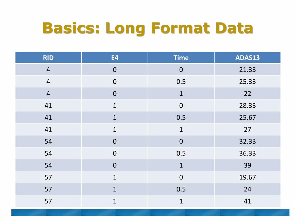
Basics: Long Format Data

RID E4 Time ADAS13

4 0 0 21.33

4 0 0.5 25.33

4 0 1 22

41 1 0 28.33

41 1 0.5 25.67

41 1 1 27

54 0 0 32.33

54 0 0.5 36.33

54 0 1 39

57 1 0 19.67

57 1 0.5 24

57 1 1 41

Basics: Terminology

▪ Between-person factors/effects

– Variables that change between people

– Example: sex, baseline age, E4 carrier status

▪ Within-person factors/effects

– Variables that change within person

– Example: time

▪ Often interested in both between- and within- person factors as well as interactions between the two

Repeated Measures ANOVA

▪ Generally assumes balanced design (no missing data)

▪ Null hypothesis: means are all equal

▪ Alternative hypothesis: at least two means are different

▪ Assumptions– Similar to ANOVA (normality of residuals,

constant variance across groups)

– Added assumption: sphericity (variances of differences between all possible pairs of within-level conditions are the same)

Repeated Measures ANOVA in SAS

proc glm data=adni_wide;

class e4;

model adas_bl--adas_m24 = e4/nouni;

repeated time 5 (0 0.5 1 1.5 2)/printe;

run;

No univariate models for each outcome (meaningless for repeated measures analysis)

5 outcome assessments Levels of time (in years)

Requests tests of sphericity

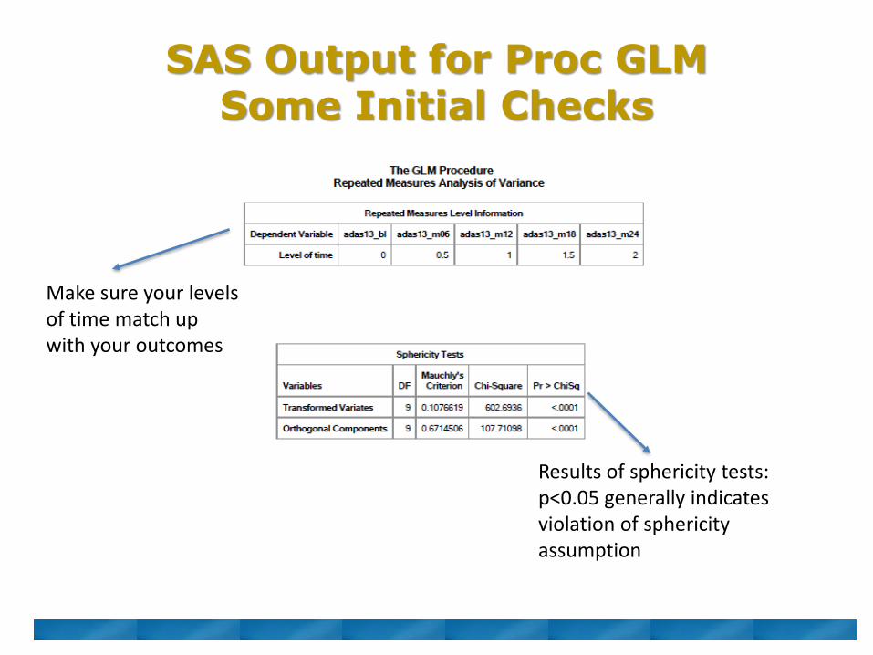
SAS Output for Proc GLM Some Initial Checks

Make sure your levels of time match up with your outcomes

Results of sphericity tests: p<0.05 generally indicates violation of sphericityassumption

SAS Output – Within person Multivariate tests

Time is significant

Time*E4 is significant

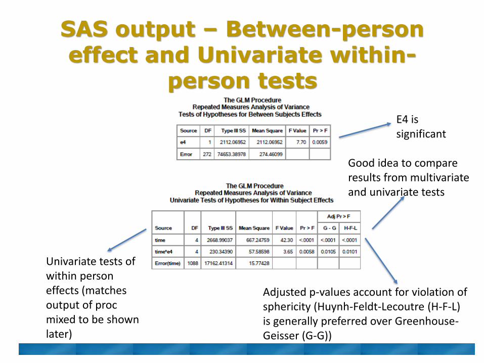
SAS output – Between-person effect and Univariate within-

person tests

E4 is significant

Univariate tests of within person effects (matches output of procmixed to be shown later)

Adjusted p-values account for violation of sphericity (Huynh-Feldt-Lecoutre (H-F-L) is generally preferred over Greenhouse-Geisser (G-G))

Good idea to compare results from multivariate and univariate tests

Mixed Effects Regression (Mixed Model): Notation

▪ Let Yij = outcome for ith person, jth

measurement

▪ Let Y be a vector of all outcomes for all subjects

▪ X is a matrix of independent variables (such as E4 carrier or time)

▪ Z is a matrix associated with random effects

Mixed Model Formulation

• Y = X + Z +

• are the “fixed effect” parameters▫ Similar to the coefficients in a regression model

▫ Coefficients tell us how variables are associated with the outcome

▫ With longitudinal data, some coefficients (of time and interactions with time) will also tell us how variables are associated with change in the outcome

• are the “random effects”, ~N(0,)

• are the errors, ~N(0,R)▫ simple example: R= 2

Random Effects

▪ Why use them?

– Not everybody responds the same way (even people with similar demographic and clinical information respond differently)

– Want to allow for random differences in baseline level and possibly rate of change that remain unexplained by the covariates

Random Effects Cont.

▪ Way to think about them– Bins with numbers in them

– Every person draws a number from each bin and carries those numbers with them

– Predicted outcome based on “fixed effects” adjusted according to a person’s random numbers

– Similar to residuals ( are residuals for each observation, while are residuals for person level data)

Random Effects Cont.

▪ Accounts for correlation in observations

▪ Correlation structures

– Compound symmetry (common within-individual correlation)

• Most common structure for repeated measures at the same visit

– Autoregressive (AR)

• Each assessment most strongly correlated with previous one

– Unstructured (most flexible)

Assumptions of Model

▪ Linearity

▪ Homoscedasticity (constant variance)

▪ Errors are normally distributed

▪ Random effects are normally distributed

▪ Typically assume Missing at Random (MAR)– Missingness is statistically unrelated to the

variable itself

– May be related to other variables in data set

Determining best covariance structure

▪ Can compare models fit with different covariance structures

▪ Compare AIC and pick model with the smallest AIC

▪ Only valid when maximum likelihood is the method of estimation (in SAS, you must change the method, since the default is something different)

▪ We’ll see more in the example

Interpretation of parameter estimates

• Main effects▫ Continuous variable: average association of one unit

change in the independent variable with the baseline level of the outcome

▫ Categorical variable: how baseline level of outcome compares to “reference” category

• Time • Average annual change in the outcome for “reference individual”

• Interactions with time▫ How change varies by one unit change in an independent

variable

• Covariance parameters▫ Measure of between-person variability (random effects)▫ Measure of within-person variability (residual variance)

Graphical Tools for Checking Assumptions

▪ Scatter plot– Plot one variable against another one (such as

random slope vs. random intercept)

– E.g. Residual plot• Scatter plot of residuals vs. fitted values or a

particular independent variable

▪ Quantile-Quantile plot (QQ plot)– Plots quantiles of the data against quantiles

from a specific distribution (normal distribution for us)

Residual Plot

Ideal Residual Plot

- “cloud” of points

- no pattern

- evenly distributed about zero

Non-linear relationship

▪ Residual plot shows a non-linear pattern (in this case, a quadratic pattern)

▪ Best to determine which independent variable has this relationship then include the square of that variable into the model

Non-constant variance

▪ Residual plot exhibits a “funnel-like” pattern

▪ Residuals are further from the zero line as you move along the fitted values

▪ Typically suggests transforming the outcome variable (ln transform is most common)

QQ-Plot

Scatter plot of random effects

Mixed Effects Models in SAS

proc mixed data=adni method=reml;

class rid e4(ref=‘0’);

model adas13=e4 time e4*time/s;

random int time/sub=rid type=un g;

repeated /sub=rid type=cs r;

run;

Options: reml (default), ml, mivque0

Requests estimates

Random intercept and slope

ID variable Specifies within-person covariance structure (compound symmetry)

Specifies between-person covariance structure (unstructured here)

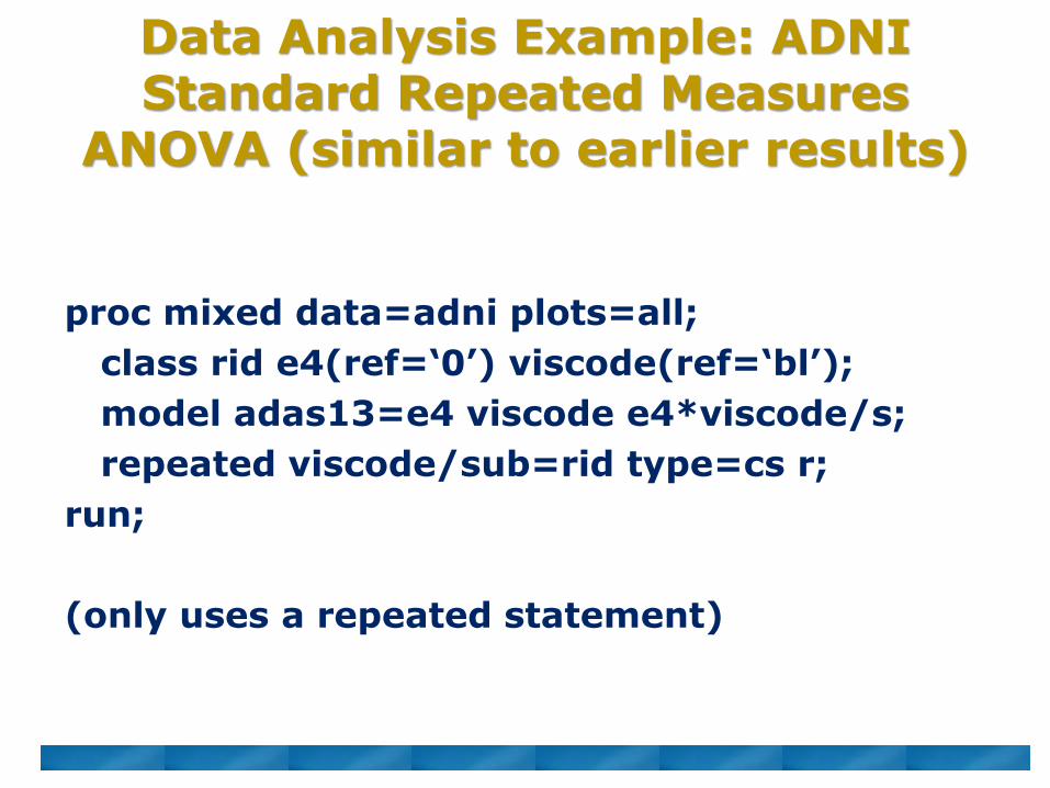
Data Analysis Example: ADNIStandard Repeated Measures

ANOVA (similar to earlier results)

proc mixed data=adni plots=all;

class rid e4(ref=‘0’) viscode(ref=‘bl’);

model adas13=e4 viscode e4*viscode/s;

repeated viscode/sub=rid type=cs r;

run;

(only uses a repeated statement)

Repeated Measures ANOVA outputproc mixed:

proc glm:

Data Analysis (Continuous time)

▪ Now want to use all available data, even if individuals are missing some visits

▪ Use time since baseline as a continuous time measure (to further account for differences in when specific visits happened)

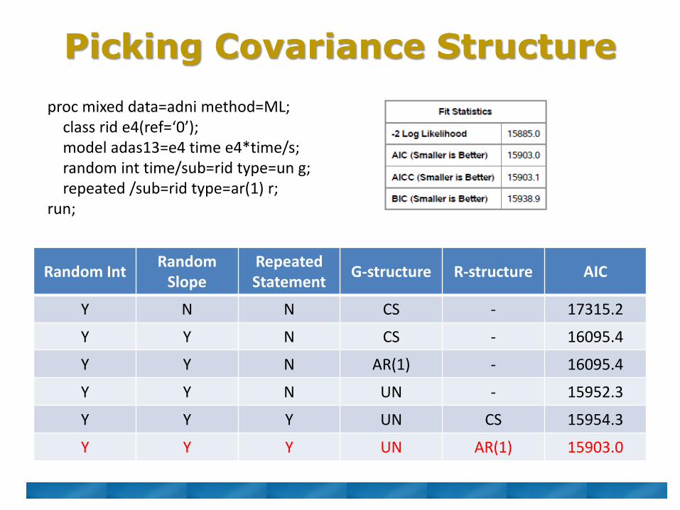
Picking Covariance Structure

Random IntRandom

SlopeRepeated Statement

G-structure R-structure AIC

Y N N CS - 17315.2

Y Y N CS - 16095.4

Y Y N AR(1) - 16095.4

Y Y N UN - 15952.3

Y Y Y UN CS 15954.3

Y Y Y UN AR(1) 15903.0

proc mixed data=adni method=ML;class rid e4(ref=‘0’);model adas13=e4 time e4*time/s;random int time/sub=rid type=un g;repeated /sub=rid type=ar(1) r;

run;

Mixed Model Output

Overall test of significance for each term in the model

At time=0 (study start), E4 non-carriers have an ADAS13 score of 16.8 on average

E4 carriers start 1.8 points higher

Non-carriers are increasing at 2.1 points per yearE4 carriers are

increasing an additional 1.5 points per year (annual increase is 2.1+1.5=3.6)

Some Diagnostics

Advanced topics

• Non-normal data▫ Generalized Estimating Equations (GEE)▫ Repeated measures models for binary, ordinal, and

count data

• Time-varying covariates• Simultaneous growth models (modeling

two types of longitudinal outcomes together)▫ Allows you to directly compare associations of

specific independent variables with the different outcomes

▫ Allows you to estimate the correlation between change in the two processes

Summary

▪ Longitudinal studies often result in repeated assessments on individuals

▪ Repeated measures ANOVA and mixed effects regression models are main strategies for analysis

▪ Mixed models can be more flexible than standard repeated measures ANOVA models

▪ SAS can fit both types of models

Help is Available

▪ CTSC Biostatistics Office Hours

– Every Tuesday from 12 – 1:30 in Sacramento

– Sign-up through the CTSC Biostatistics Website

▪ EHS Biostatistics Office Hours

– Every Monday from 2-4 in Davis

▪ Request Biostatistics Consultations

– CTSC - www.ucdmc.ucdavis.edu/ctsc/

– MIND IDDRC -www.ucdmc.ucdavis.edu/mindinstitute/centers/iddrc/cores/bbrd.html

– Cancer Center and EHS Center