Longitudinal Data Analysis for Social Science Researchers Thinking About Event Histories

Longitudinal Data Analysis for Social Science Researchers

Thinking About Event Histories

www.longitudinal.stir.ac.uk

DURATIONS

In simple form –

“Time to an EVENT”

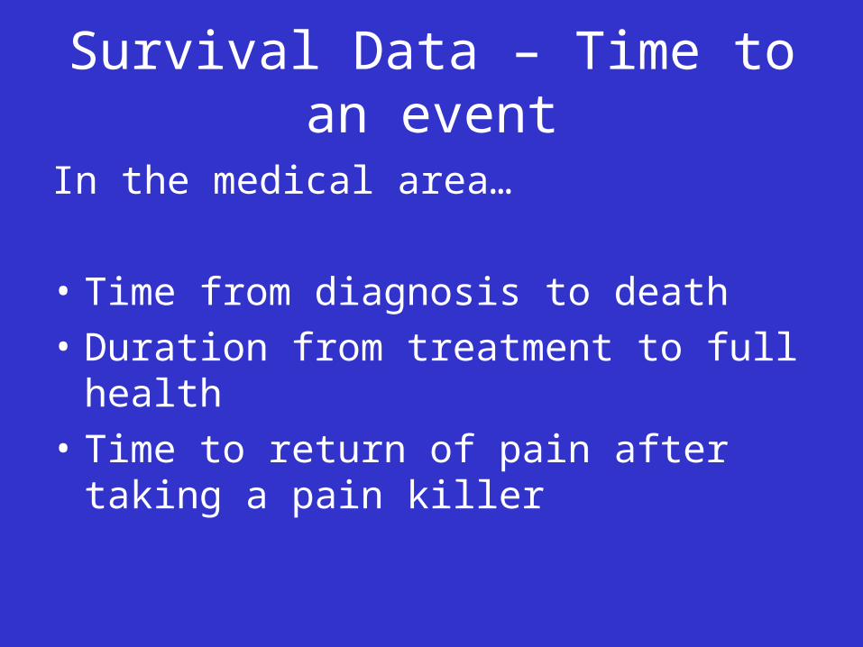
Survival Data – Time to an event

In the medical area…

• Time from diagnosis to death

• Duration from treatment to full health

• Time to return of pain after taking a pain killer

Survival Data – Time to an event

Social Sciences…

• Duration of unemployment

• Duration of housing tenure

• Duration of marriage

• Time to conception

Start of Study End of Study

0 1

0

0

1

1

t1 t2 t3

A

B

C

These durations are a continuous Y so why can’t we

use standard regression techniques?



Two examples of when we can

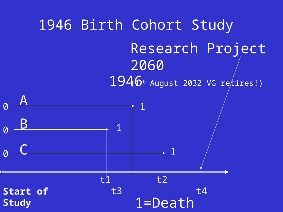
Start of Study

0 1

0

0

1

1

t1 t2 t3 t4

1946

1946 Birth Cohort Study

Research Project 2060(1st August 2032 VG retires!)

1=Death

A

C

B

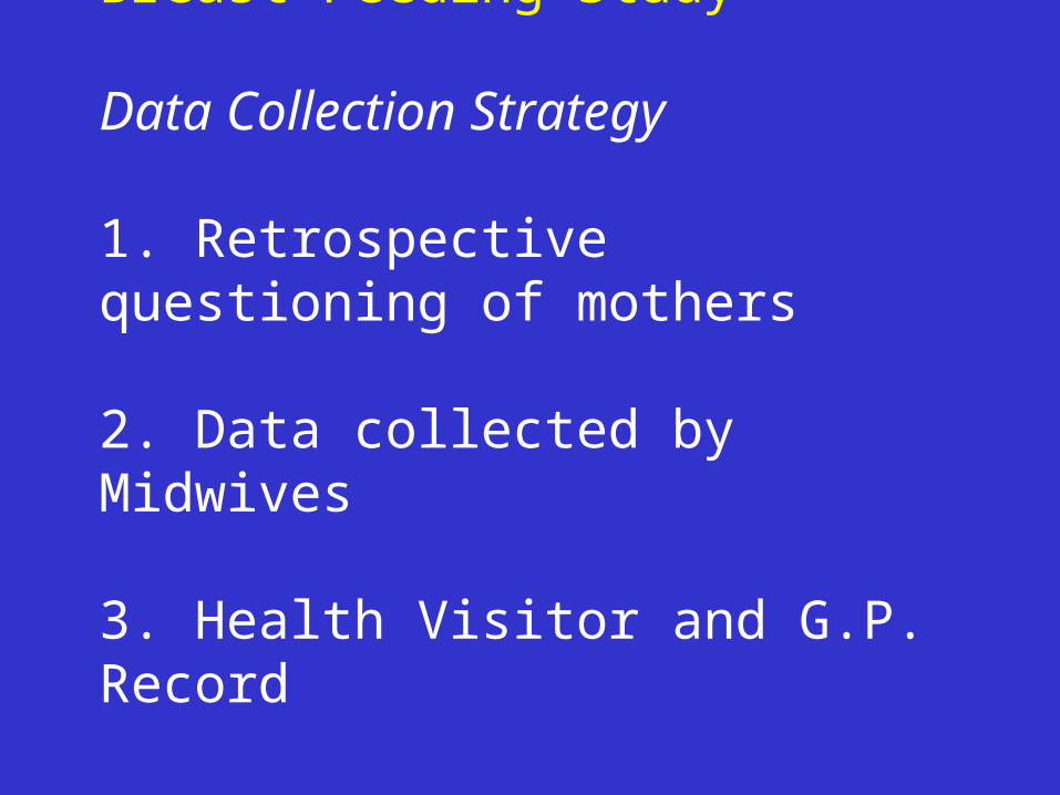
Breast Feeding Study –

Data Collection Strategy

1. Retrospective questioning of mothers

2. Data collected by Midwives

3. Health Visitor and G.P. Record

Birth

1995

Start of Study


Age 6

2001

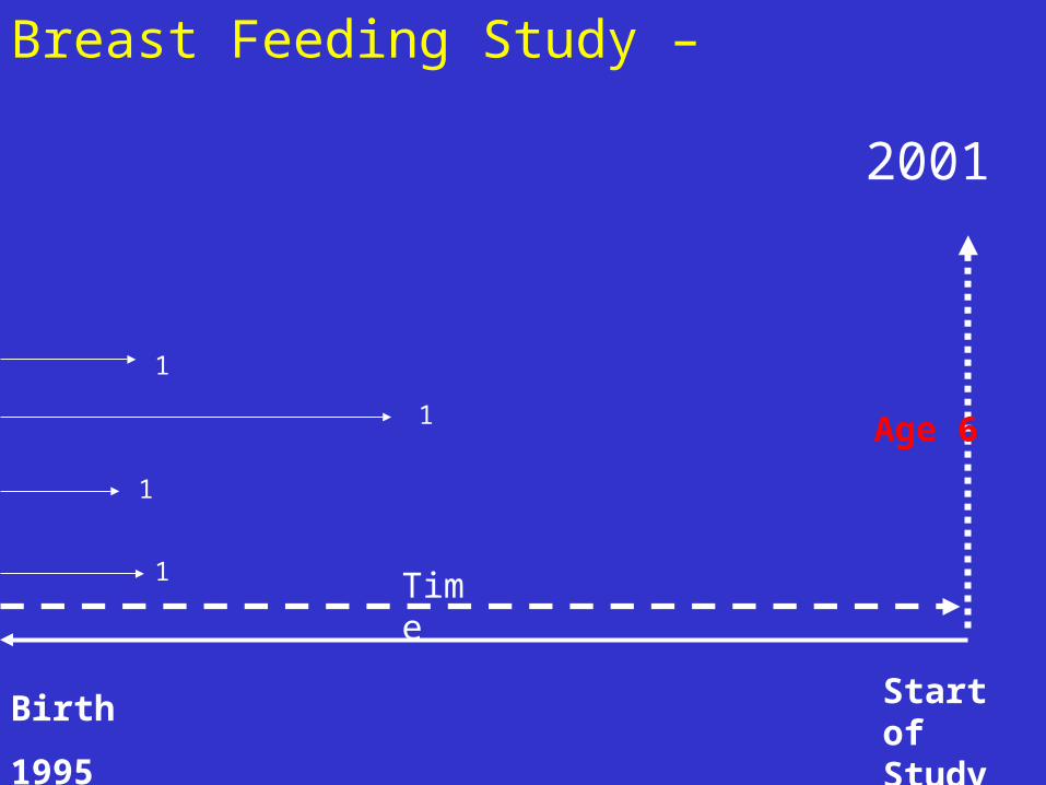
Birth

1995

Start of Study


Age 6

2001

1

1

1

1 Time



We can. It might be better to model the log of Y however. These models are sometimes known as ‘accelerated life models’.

These durations are a continuous Y so why can’t we use standard regression techniques?

Here we have censored observations. An old guideline used to be that if less than 10% of observations were censored then a standard regression approach was okay. However, you’d have trouble getting this past a good referee and there is now no excuse given that techniques are widely understood and suitable software is available.

Accelerated Life Model

Loge ti = x1i+ei

constant

explanatory variable

error termBeware this is log t

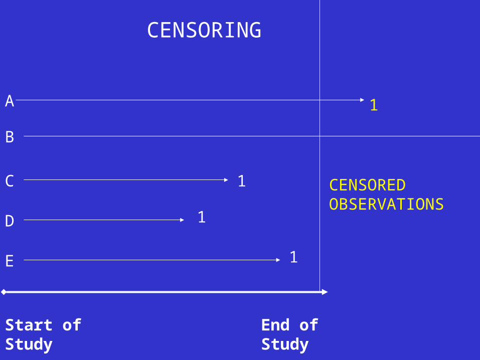
Start of Study End of Study

C 1

D

E

1

1

1

B

CENSORED OBSERVATIONS

A

CENSORING

Cox Regression(proportional hazard model)

is a method for modelling time-to-event data in the presence of censored cases

•Explanatory variables in your model (continuous and categorical)

•Estimated coefficients for each of the covariates

•Handles the censored cases correctly

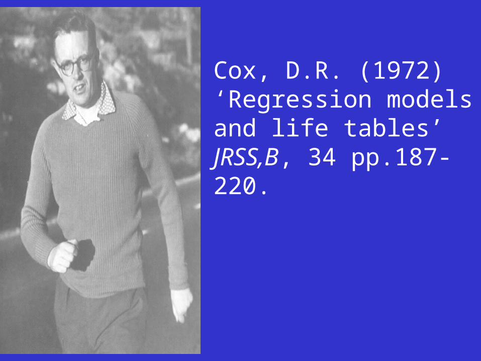
Cox, D.R. (1972) ‘Regression models and life tables’ JRSS,B, 34 pp.187-220.

Event History with Cox Model

• No longer modelling the duration

• Modelling the Hazard

• Hazard: measure of the probability that an event occurs at time t conditional on it not having occurred before t

• A more technical account follows later on!

An Example

• Duration of first job after leaving education

• Data from the BHPS

• 15,401 individual records

• 11,061 (72%) failures i.e. job spell ended

• 4,340 (28%) censored – no information on exact end of first job (e.g. still in job)

• Time in months

• Mean 78; s.d.102; min 1; max 793 (66 years)

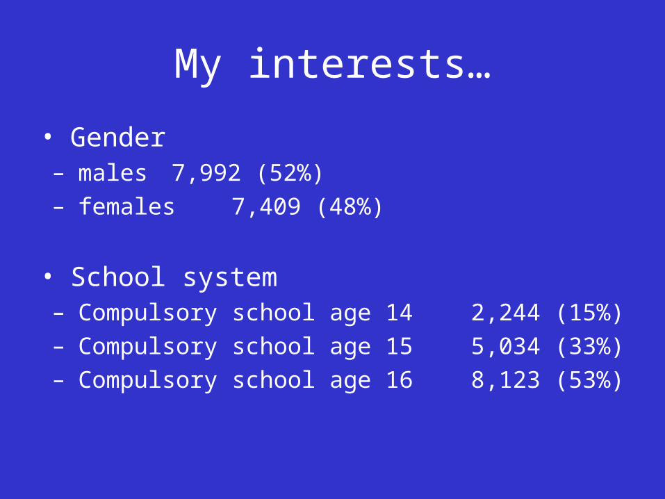
My interests…

• Gender – males 7,992 (52%) – females 7,409 (48%)

• School system– Compulsory school age 14 2,244 (15%)– Compulsory school age 15 5,034 (33%)– Compulsory school age 16 8,123 (53%)

What is the data structure?

pid start time

end time

duration gender cohort censored

The row is a person

The tricky part is often calculating the duration

Remember we need an indicator for censored cases

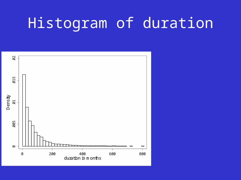
Histogram of duration0

.00

5.0

1.0

15

.02

De

nsity

0 200 400 600 800

duration in months

Descriptive Analysis DurationsMonths

• Gender Mean Median– males 89 44– females 66 39

• School system– Compulsory school age 14 146 77– Compulsory school age 15 106 71– Compulsory school age 16 42 25

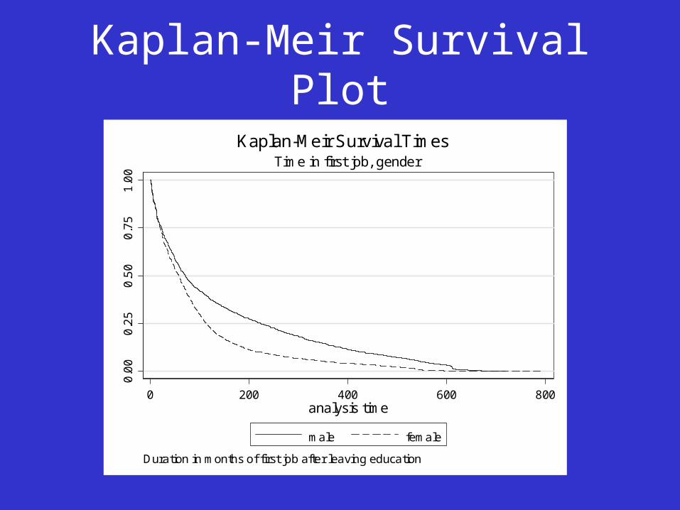
Kaplan-Meir Survival Plot0

.00

0.2

50

.50

0.7

51

.00

0 200 400 600 800

analysis time

male female

Duration in months of first job after leaving education

Time in first job, genderKaplan-Meir Survival Times

Kaplan-Meir Survival Plot

0.00

0.25

0.50

0.75

1.00

0 200 400 600 800

analysis time

age 14 leavers age 15 leavers

age 16 leavers

Duration in months of first job after leaving education

Time in first job, genderKaplan-Meir Survival Times

A Cox’s Regression –(Hazard Model)

• This is in the st suite in STATA

• You must tell STATA what is the duration variable and what is the censor variable

stset duration, failure(status)

A Cox’s Regression –(Hazard Model)

• Think of this as being similar to a logit model.

• One way of fixing this conceptually is that there is a binary response but we are interested in the time to this outcome.

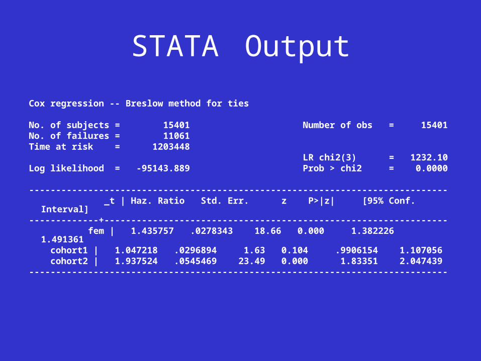
STATA Output

Cox regression -- Breslow method for ties

No. of subjects = 15401 Number of obs = 15401No. of failures = 11061Time at risk = 1203448 LR chi2(3) = 1232.10Log likelihood = -95143.889 Prob > chi2 = 0.0000

------------------------------------------------------------------------------ _t | Haz. Ratio Std. Err. z P>|z| [95% Conf. Interval]-------------+---------------------------------------------------------------- fem | 1.435757 .0278343 18.66 0.000 1.382226 1.491361 cohort1 | 1.047218 .0296894 1.63 0.104 .9906154 1.107056 cohort2 | 1.937524 .0545469 23.49 0.000 1.83351 2.047439------------------------------------------------------------------------------

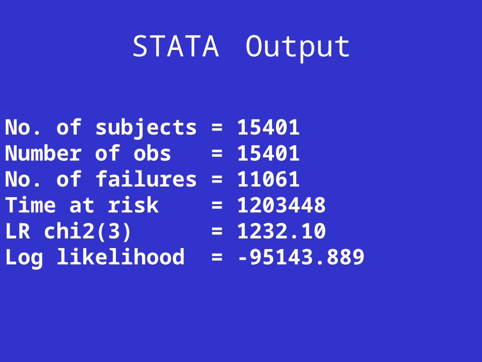
STATA Output

No. of subjects = 15401 Number of obs = 15401No. of failures = 11061Time at risk = 1203448LR chi2(3) = 1232.10Log likelihood = -95143.889

STATA Output


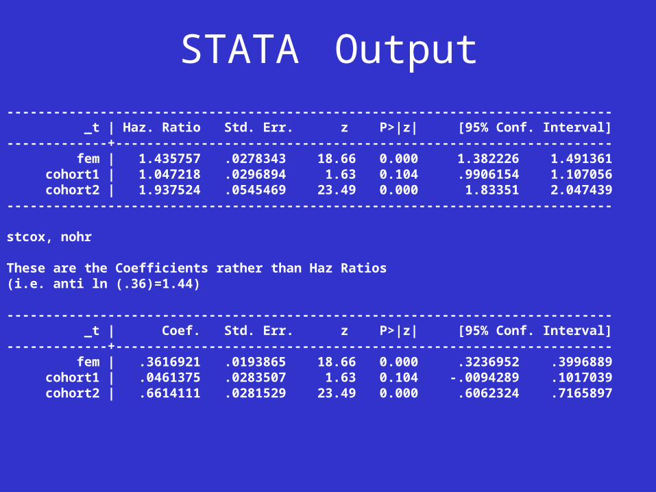
STATA Output


stcox, nohr

These are the Coefficients rather than Haz Ratios(i.e. anti ln (.36)=1.44)

------------------------------------------------------------------------------ _t | Coef. Std. Err. z P>|z| [95% Conf. Interval]-------------+---------------------------------------------------------------- fem | .3616921 .0193865 18.66 0.000 .3236952 .3996889 cohort1 | .0461375 .0283507 1.63 0.104 -.0094289 .1017039 cohort2 | .6614111 .0281529 23.49 0.000 .6062324 .7165897

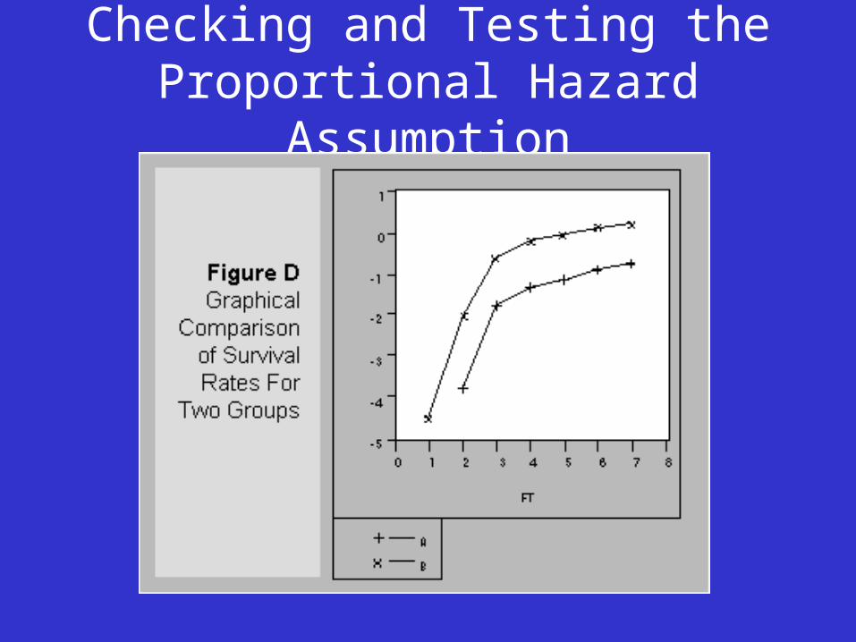
Checking and Testing the Proportional Hazard Assumption

• Key assumption is that the hazard ratio is proportional over time.

• More on this in Prof Wright’s talk.

• See also (see ST (manual) p.142 - 147 for a discussion).

• A simple visualisation might help.



.01

.02

.03

.04

Sm

oot

hed

ha

zard

fun

ctio

n

0 200 400 600 800analysis time

fem=0 fem=1

Cox proportional hazards regression


A simple example with one X var Time: Rank(t) ---------------------------------------------------------------- | rho chi2 df Prob>chi2 ------------+--------------------------------------------------- fem | 0.11224 142.09 1 0.0000 ------------+--------------------------------------------------- global test | 142.09 1 0.0000 ----------------------------------------------------------------

Ho: Fem=0 is proportional to Fem=1

Reject this null hypothesis.

See [ST] pg. 142 and more in Professor Wright’s talk!

Treatment of tied durations• If time could be measured on a true continuous scale

then no observations would be tied.

• In reality because of the resolution (or scale) that we measure time on there may be tied observations.

• The basic problem is this affects the size of the risk set - we don’t know who left first.

• There are various methods for handling this the default is Breslow; this is okay if there are not too many ties (see ST (manual) p.118 for a discussion of options).

Event history data permutations

• Single state single episode

– e.g. duration in first post-school job till end

– analogous to a logit framework

• Single episode competing risks

– e.g. duration in job until

– promotion / retire / unemp

– Analogous to a multinomial logit framework

Event history analysis software

SPSS – very limited analysis optionsSTATA – wide range of pre-prepared methodsSAS – as STATAS-Plus/R – vast capacity but non-introductoryTDA – simple but powerful freewareMLwiN; lEM; {others} – small packages

targeted at specific analysis situations

[GLIM / SABRE – some unique options]

Discrete Time

“We believe that discrete-time methods are simply more appropriate for much of the event-history data that are currently collected because, for logistical and financial reasons, observations are often made in discrete time” (Willet and Singer 1995).

Discrete Time

• In a discrete time model the dependent variable is a binary indicator

• Therefore it can be fitted in standard software

Discrete Time

We observe this woman until she experiences the event (marriage)

pid start age end age

001 16 21

She need a row for each year –

Sometimes this is called person-period format

Data Structure

Pid Y Age

001 0 16

001 0 17

001 0 18

001 0 19

001 0 20

001 1 21

Discrete Time

Discrete time approaches are often appropriate when analysing social data collected at ‘discrete’ intervals

Being able to fit standard regression models is an obvious attraction

Another event history data permutation

Another more complex situation is analysing

•Multi-state multi-episode

–e.g. adult working life histories

Paul will show an example of the state-space in his talk

Social Science Event Histories:

• Comment: Potentially powerful techniques – however in practice they are often trickier to operationalise with ‘real’ social science data. Neat examples are often used in textbooks!

• In particular: – Many research applications have concentrated on

quite simplistic state spaces (e.g. working V not in work)

– Incorporating many explanatory factors can be difficult – time constant V time-varying; and duration data V panel data.


• In particular:

– Many research applications have concentrated on quite simplistic state spaces (e.g. working V not in work)

– Incorporating many explanatory factors can be difficult – time constant V time-varying


• Is an event history analysis really what we need?

• Are we really interested in the ‘time’ to an event?

• Often a panel modelling approach may be more appropriate given our substantive interest

Documents

Longitudinal Data Analysis for Social Science Researchers Thinking About Event Histories