Embed Size (px)
Citation preview

1. Report No.
FHW NTX -03/2100-1 I 2. Government Accession No.
4. Title and Subtitle
LONG-TERM STRENGTH OF COMPACTED HIGH-PI CLAYS
7. Author(s)
Charles Aubeny and Robert Lytton 9. Perfonning Organization Name and Address
Texas Transportation Institute The Texas A&M University System College Station, Texas 77843-3135
12. Sponsoring Agency Name and Address
Texas Department of Transportation Research and Technology Implementation Office P. O. Box 5080 Austin, Texas 78763-5080
15. Supplementary Notes
Technical Report DocumentatIon PlIlle
3. Recipient's Catalog No.
5. Report Date
February 2003 6. Perfonning Organization Code
8. Perfonning Organization Report No.
Report 2100-1 10. Work Unit No. (TRAIS)
II . Contract or Grant No.
Project No. 0-2100
13. Type of Report and Period Covered
Research: September 2000-December 2002 14. Sponsoring Agency Code
Research performed in cooperation with the Texas Department of Transportation and the U.S. Department of Transportation, Federal Highway Administration. Research Project Title: Long-Term Strength Properties of High-PI Clays Used in Embankment Construction 16. Ab tracl
Moisture infiltration into earth slopes and structures constructed of high-plasticity clays will lead to a reduction in soil suction and strength that can ultimately result in stability failure. This research presents a rational analysis of this process that: establishes a relationship between soil suction and strength, and provides a framework for predicting the time rate of strength loss due to moisture infiltration into an earth mass. This research utilizes a generalized form of the Mohr-Coulomb failure criterion to characterize the effects of suction on soil strength. A diffusion equation governs changes in soil moisture and suction. This equation is in general non-linear for unsaturated soils; however, this research uses a linearized formulation through appropriate transformation of variables. This research also presents methods for estimating the necessary material parameters needed for input into the moisture diffusion model. The suction-strength relationships and moisture diffusion analyses are applied to back-analyzing a number of shallow slope failures in Texas high-PI (plasticity index) clays. The moisture diffusion analysis is also extended to typical Texas Department of Transportation earth- retaining structures to predict decreases in suction during the life of these structures. Based on these suction predictions, estimates of soil strength within an earth structure as a function of location and time are possible.
17. Key Words 18. Distribution Statement
Clays, Slopes, Moisture Diffusion, Cracking, Earth Structures
No restrictions. This document is available to the public through NTIS:
19. Security Classif.(ofthis report)
Unclassified
Form DOT F 1700.7 (8-72)
National Technical Information Service 5285 Port Royal Road Springfield, Virginia 22161
1
20. Security Classif.(ofthis page)
Unclassified
Reproduction of completed page authoriz
21. No. of Pages
100 I 22. Price


LONG-TERM STRENGTH STRENGTH OF COMPACTED HIGH-PI CLAYS
by
Charles Aubeny Assistant Professor
Texas A&M University
and
Robert Lytton Professor
Texas A&M University
Report 2100-1 Project Number 0-2100
Research Project Title: Long-Term Strength Properties of High-PI Clays U sed in Embankment Construction
Sponsored by the Texas Department of Transportation
In Cooperation with the U. S. Department of Transportation Federal Highway Administration
February 2003
TEXAS TRANSPORTATION INSTITUTE The Texas A&M University System College Station, Texas 77843-3135


DISCLAIMER
The contents of this report reflect the views of the authors, who are responsible for the
facts and the accuracy of the data presented herein. The contents do not necessarily reflect the
official view or policies of the Federal Highway Administration (FHWA) or the Texas
Department of Transportation (TxDOT). This report does not constitute a standard,
specification, or regulation. The engineer in charge was Charles Aubeny, P.E., (Texas, # 85903).
v

ACKNOWLEDGMENTS
This project was conducted in cooperation with TxDOT and FHW A. The authors would
like to express their appreciation to Project Director George Odom and Project Coordinator Mark
McClelland, from the Texas Department of Transportation, for their support and assistance
throughout this project.
VI

TABLE OF CONTENTS
Page
List of Figures ...•....................................•..........................................•......................•.•••...........•.... ix List of Tables ..•...•..........................•.....•.•..................................•...•.................•........•...............•..... x Chapter 1: Introduction ..•...........•.....•.•.................................................................•........•.........••• 1 Chapter 2: Soil Suction and Strength •......................................•................•......••......•................ 5
Matric, Total, and Osmotic Suction •............•..........•••...•........•.....•.....•..•.•..............................• 5 Units of Suction .•••.•.••...•..•............••.•..•........••..........••.................•.........•.......•...........•.........•.....• 6 Relation between Soil Suction and Strength .........•...•.....•.•...•..........•..................................... 7 Example Strength Calculations .•........•..•.•.......•..••......•.......•.....•.........•...•.•.............................. 9
Chapter 3: Moisture Diffusion through Clay .....•.........•.............•.......•............•.•...•....•.....•...... 11 Overview .•......•........................................•..•.................•••..•.........•.••....•••.•........•..............•........ 11 Mitchell's Formulation for Moisture Diffusion ..................•...•...........•................................ 11
The Diffusion Coefficient ex. ••••••••••••••••••••••••••••••••••••••••••••••••••••••••••••••••••••••••••••••••••••••••••••••••• 11 Laboratory Determination of ex. •••••••••••••••••••••••••••••• ••••••••••••••••••••••••••••••••••••••••••••••••••••••••••••••• 14
General Formulation for Diffusion ...•...................................................•............................... 16 Formulation for Steady Flow ................................................................................................ 16 Formulation for Unsteady Flow ............................................................................................ 17 Framework for Solution of Generalized Diffusion Problem ................................................ 18
Experimental Determination of Diffusion Properties ......................................................... 19 Soil Tested ............................................................................................................................ 19 Equipment and Procedures ................................................................................................... 19 Data Interpretation ................................................................................................................ 21 Results ................................................................................................................................... 23
Correlation to Index Properties .....•.•.........•...............•........•.....•.....•.....•.•.....•.•.....•....•...•..•.... 26 Evaluation of ex. from Various Sources ................................................................................. 27 Data Evaluation ..................................................................................................................... 29
Chapter 4: Analysis of Slopes ...............•....................•......•.••.•.......•..................••...................... 33 Stability" Analysis ..•.•..........•.....•...............•..••.•••••••.•••••..•..•.....•................•.....................•........•. 33
Pore-Water Pressure .............................................................................................................. 33 Soil Strength .......................................................................................................................... 35 Stability Analysis .................................................................................................................. 35 Evaporation and Infiltration .................................................................................................. 36
Case Histories in Texas High-Plasticity Clays ...•.•••.........................•...•.•.•..•....•..............•....• 36 Material Parameters .............................................................................................................. 37 Back-Analysis ....................................................................................................................... 40
Commentary on Slope Stability Analyses ...••••.•..•.....•...•...•...•...•........................................... 40 Evidence of a Flow Condition .............................................................................................. 40 Strength Degradation ............................................................................................................ 43 Wet Limit of Suction ............................................................................................................ 43 Apparent Phreatic Surface .................................................................................................... 44
Time Rate of Failure .........................................•..••.••••••.•.•......•......••....•.......•.••••.•.....••............ 44 Moisture Diffusion Predictions ............................................................................................. 45 Commentary on Moisture Diffusion Analyses ..................................................................... 50
vii

Conclusions .............................................................................................................................. 52 Chapter 5: Retaining Structures ............................................................................................... 55
Typical Designs ....................................................................................................................... 55 Boundary Conditions .............................................................................................................. 56 Initial Conditions .................................................................................................................... 58 Finite Element Model ............................................................................................................. 58 Moisture Diffusion for Typical Selected Cases ..................•..............••................................• 59 Use of Suction Prediction Analyses ...................•.......•.....•.•.............................•....•.........••.•..• 73
Chapter 6: Summary and Conclusions ..................................................................................... 77 References .................................................................................................................................... 79 Appendix: Moisture Diffusion Test Summary ........................................................................ 81
Vll1
LIST OF FIGURES
Page
Figure 1. The pF Suction Scale ...................................................................................................... 7 Figure 2. Schematic for Dry End Test. ........................................................................................ 15 Figure 3. Analytical Solution for Dry End Test. .......................................................................... 16 Figure 4. Typical Experimental Results for Dry End Test. ......................................................... 24 Figure 5. Empirical Correlations of Index Properties to Clay Permeability ................................ 27 Figure 6. Definition Sketch for Shallow Slope Stability Analysis .............................................. 34 Figure 7. Definition Sketch for Intact Slope Moisture Diffusion Mode1. .................................... 46 Figure 8. Analytical Solutions for Moisture Infiltration into a Slope .......................................... 47 Figure 9. Analytical Model for Moisture Diffusion into Cracked Slope ..................................... 49 Figure 10. Typical TxDOT Earth-Retaining Structure ................................................................ 55 Figure 11. Boundary and Initial Suctions for Moisture Diffusion Analyses ............................... 57 Figure 12. Definition Sketch for Suction Predictions .................................................................. 60 Figure 13. Suction versus Time for Structure with Aspect Ratio 4H:IV and Uo=5 ..................... 61 Figure 14. Suction versus Time for Structure with Aspect Ratio 4H: 1 V and Uo=4 ..................... 62 Figure 15. Suction versus Time for Structure with Aspect Ratio 4H:IV and Uo=3 ..................... 63 Figure 16. Suction versus Time for Structure with Aspect Ratio 4H: 1 V and Uo=2 ..................... 64 Figure 17. Suction versus Time for Structure with Aspect Ratio 4H:IV and Uo=1. .................... 65 Figure 18. Suction versus Time for Structure with Aspect Ratio 4H:IV and Uo=0.5 .................. 66 Figure 19. Suction versus Time for Structure with Aspect Ratio 8H:IV and Uo=5 ..................... 67 Figure 20. Suction versus Time for Structure with Aspect Ratio 8H: 1 V and Uo=4 ..................... 68 Figure 21. Suction versus Time for Structure with Aspect Ratio 8H:IV and Uo=3 ..................... 69 Figure 22. Suction versus Time for Structure with Aspect Ratio 8H:IV and Uo=2 ..................... 70 Figure 23. Suction versus Time for Structure with Aspect Ratio 8H: 1 V and Uo= 1 ..................... 71 Figure 24. Suction versus Time for Structure with Aspect Ratio 8H: 1 V and Uo=0.5 .................. 72
.' IX

--------------------
LIST OF TABLES
Page
Table 1. Soil Sample Index - Waco Site ..................................................................................... 20 Table 2. Summary of Moisture Diffusion Tests .......................................................................... 25 Table 3. Moisture Diffusion Coefficient a from Different Sources ............................................ 28 Table 4. Diffusion Coefficients Inferred from Paris Clay Slope Failure Data (11 ) ..................... 30 Table 5. Diffusion Coefficients Inferred from Beaumont Clay Slope Failure Data (11) ............ 31 Table 6. Site Data for Shallow Slides in Paris Clays (11) ........................................................... 38 Table 7. Site Data for Shallow Slides in Beaumont Clays (11) ................................................... 39 Table 8. Back-Analyzed Failures in Paris Clays ......................................................................... 41 Table 9. Back-Analyzed Failures in Beaumont Clays ................................................................. 42
x

CHAPTER 1: INTRODUCTION
High-plasticity clays occur in many areas of Texas and often offer the most economical
material alternative for construction of highway embankments. When constructed with proper
moisture and compaction control, embankments constructed of plastic clays can perform
adequately with regard to overall stability. However, experience shows that the outer layers of
these embankments can experience dramatic strength loss. Softening of the surficial soils can
begin soon after construction and continue for decades. The consequent sloughing and shallow
slide failures represent a significant maintenance problem for TxDOT. The problem of strength
loss in high-plasticity clay soils can also impact other structures such as retaining walls,
pavements, and riprap. This report presents the results of research that develops an approach for
estimating soil strength loss as a function of time and space for typical slopes and earth structures
used in TxDOT projects.
The soils in the slopes and earth structures described above are unsaturated.
Accordingly, soil suction contributes substantially to the shear strength of the soil, and changes
in soil strength can largely be attributed to changes in suction. The magnitude of soil suction in
clayey soils compacted at or near the optimum moisture content is typically high (on the order of
u = 4 pF) with a correspondingly high shear strength. Over time moisture can migrate into the
earthfill, with a concomitant decrease in the magnitude of suction and strength. The amount of
strength loss will depend on environmental moisture conditions, while the rate of strength loss
will be governed by the moisture diffusion properties of the soil.
A framework for predicting strength degradation over time must address the two major
issues: suction and its relationship to soil strength, and the time rate of moisture infiltration into a
soil mass. Estimating soil strength from suction requires a basic understanding of the principles
of suction, and knowledge of the constitutive laws relating suction and mechanical stress to soil
strength. Chapter 2 of this report covers these topics. Predicting the rate of moisture infiltration
into an unsaturated soil mass requires an analytical model for describing moisture flow through
an unsaturated soil, a means of obtaining the required material parameters as inputs to the model,
and solutions to the boundary value problem for moisture diffusion. Chapter 3 covers the first
two of the above topics, the analytical model and methods for estimating the necessary input
parameters. Solution of the boundary value problem depends on the geometry of the slope or
1

earth structure under consideration. In general, moisture infiltration into slopes involves
relatively simple boundary conditions for which closed form analytical solutions are possible.
Retaining wall problems typically involve a more complex problem geometry that usually
requires recourse to numerical solutions. Chapters 4 and 5 of this report, which cover slopes and
retaining walls, respectively, present analytical solutions.
Chapter 4 presents a thorough coverage of the mechanism of shallow sliding failures in
high-PI (plasticity index) clay slopes. The first portion of this chapter outlines the slope stability
analysis in detail including the pore pressure assumptions, the suction-strength relationship, and
a description of the failure condition. The stability analysis is then applied to case histories of
slope failures in high-PI Texas clays. An important product of the review of the case histories is
an estimate of the lower bound of suction that can occur on a free surface of soil exposed to
moisture. For the cases reviewed, this lower bound showed a remarkable uniformity. The lower
bound of suction is quite important, because it establishes a lower bound to which the soil
strength can degrade, and it establishes a realistic boundary condition for moisture infiltration
analyses. The final portion of Chapter 4 addresses the time-dependent aspects of shallow slope
failures. For the case histories reviewed, the time to failure was typically on the order of 10 to
30 yr. The latter portion of Chapter 4 applies the moisture diffusion analytical framework
developed in Chapter 3 to explain these times to failure.
Chapter 5 applies the moisture diffusion analysis presented in Chapter 3 to predict the
suction loss as a function of location and time in typical TxDOT earth-retaining structures.
Unlike the shallow slope slide problem, a retaining structure can fail by a number of
mechanisms, many of which are specific to a given set of design details and site conditions.
Given this complexity, this research does not attempt to predict failure times for earth-retaining
structures. Instead it provides predictions of suction as a function of location and time for a
series of retaining-structure designs and site conditions. The predicted suction provides a basis
for predicting apparent cohesion (capp) as a function of location and time. Using this apparent
cohesion and the internal friction angle of the soil as strength input parameters, the engineer can
perform the typical analyses of retaining wall stability.
The moisture diffusion analysis used in this research requires a solution of a linear
diffusion equation which, for a complex geometry, usually involves numerical techniques such
2

as the finite element method. Finite element programs for solution of a linear diffusion equation
are widely available in commercial codes.
3


CHAPTER 2: SOIL SUCTION AND STRENGTH
Changes in soil suction over time playa critical role in strength degradation in soils
during the life of a slope or earth structure. Accordingly, it is important for a designer of these
structures to understand basic concepts of suction and how suction relates to shear strength of the
soil. The following sections of this chapter present these basic concepts.
MATRIC, TOTAL, AND OSMOTIC SUCTION
Surface tension at the air-water interface in an unsaturated soil will lead to negative water
pressures in the soil referred to as matric suction. This negative pressure directly affects the
intergranular stresses between soil particles and therefore has a strong influence on soil strength.
Higher magnitudes of suction bind the soil particles more tightly together leading to higher soil
strength. While suction always represents a negative water pressure, some authors and
references adopt a sign convention in which suction is a positive number. Provided one is
consistent, such a convention can lead to correct results. However, regardless of the sign
convention used, it is important for the soils engineer to remember that under the usual field
conditions in which the air phase is at atmospheric pressure, the water pressure in a partly
saturated soil is physically a negative value.
Matric suction in a soil varies with the soil's moisture content. The soil-moisture
characteristic curve refers to the relation between matric suction and moisture. Since the soil
moisture content typically varies during the life of an earth structure, suction will also vary. As
the soil moistens matric suction and strength will decline, and vice-versa. The laws governing
the diffusion of moisture into and out of an unsaturated soil mass parallel in many ways those for
saturated soils with which most geotechnical engineers are familiar. Hence, changes in matric
suction over time in a slope or earth structure are governed by predictable processes of moisture
diffusion through soils.
Gradients of total suction drive moisture flow through unsaturated soils (1). Matric
suction is one component of total suction. However, there is another component of total suction
that will influence moisture flow: osmotic suction. Osmotic suction relates to the tendency of
water molecules to migrate from a region of low salt concentration to that of a higher
5

concentration. The total suction (ht) in a soil is the sum of osmotic suction (n) and matric suction
(hm):
ht = n + hm (Eq. 1)
When working with suction, one must, therefore, remember that moisture flow
calculations must be in terms of total suction, while soil strength and deformation calculations
must be in terms of matric suction.
UNITS OF SUCTION
Suction can be expressed in using the usual units of water pressure; e.g., pounds per
square foot (pst) or head of water (ft). An alternative widely used measure of suction is the pF
scale, which the logarithm of the head in centimeters (cm) of water:
u(PF) = 10glO [-h( cm)] (Eq.2)
Figure 1 shows several important reference points on the pF scale for total suction. Two
particularly noteworthy reference points are the wet limit for clays and the wilting point, which
are 2.5 and 4.5 pF, respectively. These points are important since they define the lower and
upper range of suction in clays that will occur in most field situations. More specific ranges
associated with climactic regions of Texas will be presented later in this report. However, the
reference points shown in Figure 1 provide a good initial guide as to what levels of suction can
occur in clay soils.
The mathematical analysis of moisture flow through unsaturated soils is considerably
simplified when suction is expressed on a logarithmic (pF) scale rather than a natural scale. For
this reason predictions of suction over time within a soil mass are presented in terms of a pF
scale in this report. For strength calculations, suction on a pF scale must be converted to units of
pressure, making use ofEq. 2.
6

pF SUCTION SCALE
7 OVEN DRY
6 Am DRY
TENSILE STRENGTH OF 5 CONFINED WATER
WILTING POINT 4
PLASTIC LIMIT FOR CLAYS u(PF) = loglO[ -h(cm)] 3
WET LIMIT FOR CLAYS 2
LIQUID LIMIT
Figure 1. The pF Suction Scale.
RELATION BETWEEN SOIL SUCTION AND STRENGTH
Assuming a condition of no excess pressure in the pore-air phase - a reasonable
assumption when considering long-term strength - the shear strength of an unsaturated soil can
be characterized by a Mohr-Coulomb relationship of the form:
'tf = capp + a' tan ~'
where: a' ~'
net mechanical stress mechanical stress internal friction angle failure shear stress
The apparent cohesion (capp) in Eq. 3a is defined by:
Capp = - hm Ie tan~'
where: ~' = mechanical stress internal friction angle e = volumetric water content (volume waterltotal volume) I = factor ranging fromf=l tof=l/e
(Eq.3a)
(Eq.3b)
Computation of strength using Eqs. 3 is most expedient in cases for which an effective
stress analysis is to be performed, typically in cases where the net mechanical stress contributes
7

substantially to the shearing resistance. In problems involving shallow soils for which the soil
shear strength is dominated by suction, it is often useful to characterize soil strength in terms of
an unconfined shear strength (Cue). If the matric suction (hm) is known or has been estimated, the
following expression characterizes the shear strength in unconfined compression:
Cue = - hm Ie sin ~'I [1 - sin ~'] (Eq.4)
where ~', e, and/are as defined in Eq. 3. Eq. 4 is valid so long as all excess pore pressures
generated during shearing have dissipated. This is generally a valid assumption when
considering the long-term stability of slopes and earth structures. However, as full saturation is
approached during wetting of a soil, strains may develop relatively rapidly due to the final stages
of softening of the soil, in which load-induced pore pressures may be generated. In this case, a
lower bound (undrained) estimate of the unconfined compressive shear strength is:
Cue = - hm Ie sin ~'I [1 - (1 - ar) sin ~'] (Eq.5)
where: ar = is the Henkel pore pressure coefficient at failure.
A typical value of Henkel's coefficient (ar) for a compacted soil wetted to saturation is
about 1.4. A significant advantage of characterizing soil strength in terms of the unconfined
compressive strength (Eq. 5) is that the effects of load-induced pore pressures (characterized by
ar) are readily incorporated into the strength estimate.
Both Eqs. 3 and 4 require an estimate of the mechanical stress friction angle. This can be
directly measured in the laboratory, typically in a consolidated-undrained triaxial shear test with
pore pressure measurements. However, the friction angle can often be satisfactorily estimated
using an empirical correlation to the plasticity index (1):
sin ~'= 0.8 - 0.22 10glO (PI) (Eq. 6)
The factor (j) in Eqs. 3 through 5 accounts for the fact that in an unsaturated soil the
water phase does not act over the entire surface of the soil particles (2). For degrees of saturation
less than 8 < 85 percent,/is essentially equal to unity. As full saturation is approached/= lie.
F or degrees of saturation intermediate between these cases, 85 percent <8< 100 percent, I can be
8

reasonably estimated by linear interpolation. This behavior can be expressed in equation form as
follows:
s = 100 percent
S ::; 85 percent
85 percent < S < 100percent
1=1/0
1=1
I = 1 + S -85 (2.. -1) I
15 0
EXAMPLE STRENGTH CALCULATIONS
(Eq.7)
A high plasticity clay is compacted to a dry density (Yd) of93 pcfwith a matric suction
(u) 4.0 pF, and a moisture content w = 22 percent. The specific gravity (Gs) and friction angle
(~') are estimated to be 2.70 and 26 degrees, respectively. Compute the unconfined compressive
strength eu (Eqs. 4 and 5) for the following conditions: as compacted with u = 4 pF, after
saturation to u = 2 pF, and at an intermediate wetting stage with u = 3 pF.
a. As-compacted strength:
The first step is to determine the degree of saturation of the as-compacted material. This
can be done by first computing the void ratio ( e) of the soil:
e = (Gs Yw / Yd) - 1 = (2.70 x 62.4 pcf 193 pct) - 1 = 0.81
The corresponding degree of saturation (S) is computed from:
S = w Gs 1 e = (0.22)(2.70) / 0.81 = 73.3 percent.
Since the degree of saturation (8) is less than 85 percent,l= 1.0.
The volumetric water content 0 is:
o = w ( Yd 1 Yw) = 0.22 x (93 pcf/62.4 pct) = 32.8 percent
A matric suction u = 4 pF corresponds to hm = -104 cm of water or -20,500 psf. ApplyingJ, 0,
hm, and ~' in Eq. 4 yields:
eu = (20,500 pst) (1.0) (0.328) sin 26°1 (1- sin 26°) = 5250 psf
b. Saturated strength
Since the saturation (8) is 100 percent,l= 110, oriS = 1. The matric suction in units of
pressure is -100 cm of water or -205 psf. Substitution in Eq. 4 results in the following apparent
cohesion assuming no generation of excess pore pressures due to loading:
eu = (205 pst) (1.0) sin 26°1 (1- sin 26°) = 160 psf
9

If excess pore pressures are assumed to develop with a Henkel pore pressure coefficient
(ar) of 1.4, from Eq. 5 the apparent cohesion becomes:
Cu = (205 pst) (1.0) sin 26°1 [1- (1 - 1.4) sin 26°] = 76 psf
c. Strength at u = 3.0 pF
To estimate strength, one must first make an estimate of the water content (w) and degree
of saturation at the suction level in question. For matric suctions in the range u=2 to 4 pF, a
reasonable assumption is that the water content varies linearly with suction on a pF scale. The
moisture content calculations are therefore as follows:
Matric suction, u
4pF
Moisture Content (w)
22 percent (given at start of problem)
2 pF Wsat = e/Gs = 30.7 percent
The moisture content at u=3.0 pF can now be estimated by interpolation:
W3.0 = 30.7+ [(22-30.7) 1(4-2)] (3.0-2.0) = 26.3 percent
The corresponding degree of saturation (S) is computed from:
S = w Gs I e = (0.263)(2.70) I 0.81 = 87.7 percent
The volumetric water content 0 is:
0= w ( ¥w I ¥d) = 0.263 x (93pcf/62.4pct) = 39.2 percent
Since the degree of saturation is between 85 and 100 percent,f must be estimated by
interpolation. Recalling that when S=85 percentf= 1 and when S = 100 percentf= 1/0, the
appropriate interpolation is:
f= 1 + [(87.7-85) I (100-85)] (1 10.392 - 1) = 1.28.
For a matric suction u = 3.0 pF = -1,000 cm water = -2050 psf, the apparent cohesive strength
can now be estimated from Eq. 4:
Cu = (2,050 pst) (1.28) (0.392) sin 26°1 (1- sin 26°) = 800 psf
Finally, one should note that the volumetric calculations above are based on a constant
void ratio (e). In actuality, changes in void ratio will occur with changes in suction. However,
the effect is small compared with other variables in the problem. In particular, one should recall
that during the wetting process the magnitude of matric suction declines from 20,500 psf to 205
psf. Given this enormous variation in the scale of suction, secondary effects associated with void
ratio changes can be reasonably neglected in the strength calculations.
10

CHAPTER 3: MOISTURE DIFFUSION THROUGH CLAY
OVERVIEW
Changes in suction will occur as moisture infiltrates into the soil mass during the life of
an earth structure. Therefore by predicting how moisture infiltrates into a soil mass over time,
one can predict changes in suction over time at various locations within a slope or earth
structure. In contrast to flow through saturated soils, the analysis of the moisture infiltration
through unsaturated soils is nonlinear due to the dependence of permeability on suction level in
the soil. While such problems can be solved numerically, the nonlinearity introduces a number
of difficulties, particularly when attempting to interpret laboratory or field measurements. By
analyzing seepage in terms of the logarithm of suction (Eq. 2), Mitchell (4) demonstrated that a
linear analysis of flow through unsaturated soils was possible. This finding greatly simplifies
interpretation of laboratory measurements and permits analytical predictions of moisture
diffusion and suction change through a soil mass to proceed in a straightforward manner.
Mitchell's original formulation uses a fairly restrictive assumption as to how permeability
varies with suction. This research generalizes his original formulation to avoid this restriction.
A critical aspect of predicting the time rate of suction and strength degradation is
estimating the input parameters for the analytical or numerical model. This chapter presents
methods of measuring or estimating these parameters.
MITCHELL'S FORMULATION FOR MOISTURE DIFFUSION
The Diffusion Coefficient a
The rate of diffusion of liquid through a partly saturated soil is governed by the soil
permeability and by the moisture-suction characteristic curve.
Permeability is defined by Darcy's law, which in one dimension is:
v = -k d<l>/dx (Eq.8)
where: v discharge velocity
k = permeability
11

<D = total potential (total head)
x = distance
In saturated soils, the permeability (k) is essentially constant. However, in partly
saturated soils, the permeability is dependent on the degree of saturation, or in a more convenient
formulation, on the total suction (h t). Note that the total suction is related to potential by:
<D = ht + z (Eq.9)
where: z = vertical coordinate.
Laliberte and Corey (5) propose the following permeability suction relationship:
where: ko
h
ho
n
reference permeability (saturated)
total suction
total suction corresponding to reference state (approx. 6.28 ft)
material constant
(Eq. 10)
Mitchell (4) proceeds to show that, if changes in elevation (z) are small relative to the
magnitude of suction, <D = h. Further, if one assumes n = 1 :
v = - ko (ho / h) (dh /dx) (Eq. 11)
Noting that dh / h = d loge h, it follows that:
v = - (ko ho /0.434) d (IOglO h ) /dx (Eq.12)
Mitchell (4) expresses this equivalently:
v=-p du /dx (Eq. 13)
where: p = permeability parameter = - ko ho /0.434
u total suction on a pF scale = 10glO h( cm of water)
12

Although Mitchell's proposed approach is an approximation, it permits linear solution of
Laplace's equation. Hence, partly saturated seepage problems can be treated using the analytical
tools that have been established for saturated flow including flow nets, closed form analytical
solutions, and linear finite difference and finite element analyses, with the solution variable
being u(PF) instead of potential (<1».
The soil-moisture characteristic curve defines the relationship between total suction and
water content. This relation establishes the moisture storage term for unsteady partly saturated
seepage problems. Mitchell (4) defines the moisture characteristic c as the slope of the
gravimetric water content versus the logarithm of total suction curve, or if total suction is
expressed on a pF scale, the slope of the water content versus suction (pF) curve:
8=-du/dw (Eq. 14)
where: 8 slope of moisture characteristic
w gravimetric water content = weight water/weight solids
u = suction on pF scale
For purposes of a simplified analysis, Mitchell (4) proposes a linearized analysis in which
8 is constant. Data presented by Mitchell indicates that this is a reasonable assumption for pF =
2.0 to 4.0. It is well known that the soil-moisture characteristic curve can exhibit considerable
hysteresis (1); i.e., the curve differs for wetting versus drying. However, in the simplified
analyses described subsequently, hysteresis will be neglected.
By invoking the conservation of mass condition in a manner that parallels the well
known formulation for saturated flow, Mitchell (4) shows the following diffusion equation:
(Eq.lS)
where: u total suction on a pF scale
t = time
ex = diffusion coefficient = -8 p ¥w / ¥d
¥d soil dry unit weight
13
Yw unit weight of water
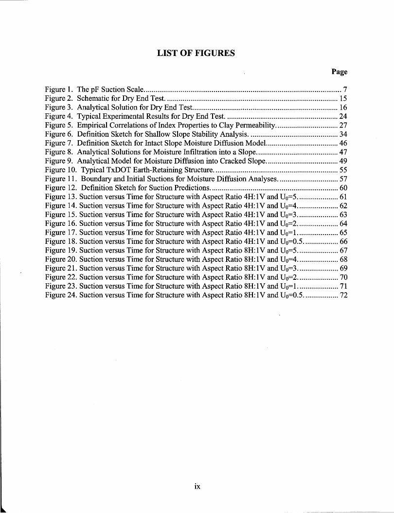
Like the coefficient of consolidation (cv) in saturated soils, the diffusion coefficient ( a) is
not a fundamental material parameter. Rather it is proportional to the ratio of two fundamental
parameters; namely, the permeability parameter (P) and the storage coefficient (1/8). As
adoption of the coefficient of consolidation (cv) is convenient in test interpretation analysis of the
consolidation of saturated soils, the coefficient (a) is likewise convenient in test interpretation
and analysis of moisture diffusion through partly saturated soils.
Laboratory Determination of a
To evaluate the diffusion coefficient (a) in the laboratory, Mitchell (4) proposed two tests
that could be performed on conventional undisturbed soil samples, such as Shelby tube samples.
Figure 2 shows the sides and one end of the sample sealed in both tests. Opening one end of the
sample permits the flow of moisture into or out of the sample. Small holes drilled into the sides
of the sample at several locations provide openings for psychrometers to measure suction. The
recent tests performed by Tang (6) at Texas A&M University (TAMU) used six thermocouple
psychrometers. By measuring suction as a function of time and location, the theory developed
above allows back-calculation of the diffusion coefficient (a).
The formulation for the drying test must consider the evaporation boundary condition at
the soil-air interface. The relevant equation proposed by Mitchell (4) is:
(Eq.l6)
14

Sealed end and sides Psychrometer measurements, u( x, t)
1 2 3 4 5 6
--.
Open end
--. Evaporation Soil sample --.
~----------------------------------.
I----·~x
~ Length,L
Figure 2. Schematic for Dry End Test.
~I Atmospheric suction, Ua
Applying Eq. 16 at the open end and a no-flow boundary condition at the closed end to
Eq. 8 leads to the following solution by Mitchell (4) for suction u(x,t) as a function of time and
coordinate in the soil sample:
(Eq.17)
where: Ua atmospheric suction
Uo initial suction in soil
a diffusion coefficient
t time
L sample length
x coordinate
he evaporation coefficient
Figure 3 shows an illustration of the general solution in terms of dimensionless variables
for a typical specimen length (L) and evaporation coefficient (he) (L = 1.31 ft, he = 16.5 ft-I).
15

Diffusion Test· Open End
0.9
i 0.8 ::::II cis $: 0.7 0 ::::II 0.6 2-C
0.5 0 :g ::::II
UJ 0.4 "tS
.~ iii 0.3 E ~
0 0.2 z
0.1
0
0 0.1 0.2 0.3 0.4 0.5 0.6 0.7 0.8 0.9
Normalized Distance, x/L
Figure 3. Analytical Solution for Dry End Test.
GENERAL FORMULATION FOR DIFFUSION
One significant restriction of Mitchell's formulation is the assumption that the coefficient
(n) in Eq. 10 must be equal to unity. A comprehensive database of exponent (n) values is
lacking, but existing data by Brooks and Corey (7) suggest that it can exceed unity for a number
of soils. A less restrictive formulation is possible by defining a function ('V) such that:
dlf/= h-n dh
If/ = loge h
If/ = h1-n
/ (l-n)
n=1
n>1
Applying Eqs. 18 to Eqs. 8 and 10 now leads to:
v = ko h; tfJ! dx
Formulation for Steady Flow
(Eq. 18a)
(Eq. 18b)
(Eq. 18c)
(Eq. 19)
The discharge velocity v is now directly proportional to the gradient of 'V; hence, the
analysis of steady seepage can proceed using linear techniques including analytical solutions,
16

flow nets, or linear numerical methods. The solution variable ('V) is readily transformed to total
suction (h) using Eqs. 18.
Formulation for Unsteady Flow
To preserve the linear form of the diffusion equation (Eq. 15), the moisture storage
relationship (Eq. 14) must satisfy certain requirements. Namely, the slope of the moisture
content-suction curve must be controlled by the same exponent (n) that governs the permeability
relationship in Eq. 10; that is:
dw -= dh
1 1 ---S h n
(Eq.20)
For the special case ofn=l, integration ofEq. 20 and solving for S leads to:
8w (Eq.21a) =--
Similar integration for the more general case of n> 1 leads to:
(Eq.21b)
This leads to the conclusion that so long as the moisture-suction relationship is governed
by the same exponent (n) as the permeability-suction relationship, the gravimetric moisture
content will be linearly related to the variable (\}l) and a linear analysis of transient seepage is
possible. A linkage between the moisture content-suction relationship and the permeability
suction relationship has long been recognized; e.g., Fredlund et al. (8). Some proposed empirical
relationships, such as Brooks and Corey (7), do not necessarily support the form ofEq. 20.
However, even if Eq. 20 is not strictly satisfied, a linearized approximation is nevertheless
possible by selecting a representative slope of the moisture-suction curve (S = 8\f' / 8w) for the
range of suction and moisture relevant to the problem at hand.
17
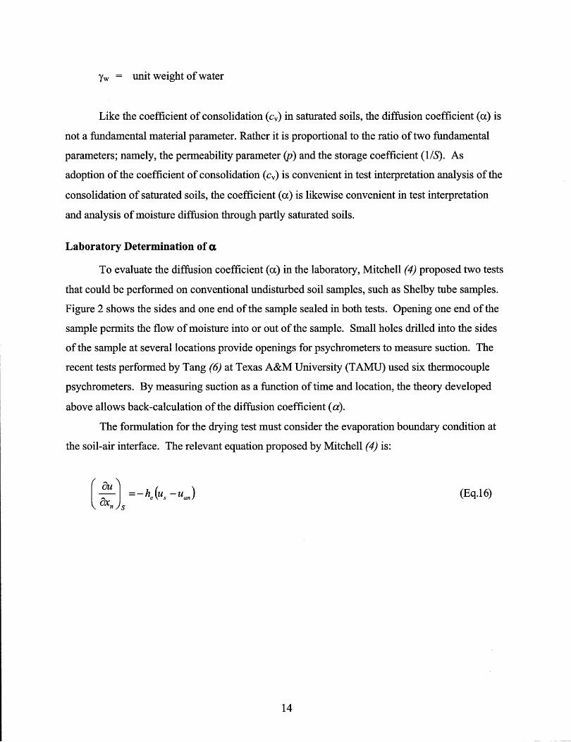
Finally, a diffusion coefficient (a) must be defined for the generalized formulation. This
can be formulated in a manner similar to the development of the original diffusion coefficient;
namely:
-8 koh;yw a = _ ......................... (Eq.22) Yd
where ko, ho, and n are defined by Eq. 10 and S is defined by Eq. 21.
The diffusion equation now becomes:
(Eq.23)
Since Eq. 23 is linear, any solutions presented previously (e.g., Eq. 17) are applicable
provided that the original solution variable (u) is replaced by the transformed variable (\}').
Framework for Solution of Generalized Diffusion Problem
With a linearized formulation for transient water flow through an unsaturated soil
established, an analysis can now proceed according to the following steps:
1. Evaluate the two relevant material parameters for the soil (a and n) using the experimental
approach that will be discussed in subsequent sections.
2. Estimate the distribution of the initial suction (hi) and the imposed boundary suction (hB) for
the problem and transform these variables to \}Ii and \}IB, respectively, using Eq. 18.
3. Solve Eq. 23 for the initial and boundary conditions prescribed in Step 2 to obtain \}I as a
function of space and time.
4. Compute the total suction h from \}I by inverting Eq. 18.
A final issue remains as to the treatment of water evaporation at an air-soil interface.
Until better data become available, the authors propose that for analytical convenience Eq. 16 be
generalized as follows:
18

(Eq.24)
The evaporation constant (he) is similar to that in Eq. 16, except that it is now defined in
terms of the generalized diffusion formulation.
The results of the test program discussed in the next section suggest that experimental
values of a are not sensitive to variations in he; hence, the investigators recommend continued
use ofEq. 24 until experimental data dictate a refinement to this approach.
EXPERIMENTAL DETERMINATION OF DIFFUSION PROPERTIES
A series of laboratory experiments performed at Texas A&M University evaluate the
validity of the analytical framework described above.
Soil Tested
Clay samples provided by the Texas Department of Transportation were utilized in the
experimental program. The soils (Table 1) had properties of a high-plasticity clay (CH): liquid
limit LL = 56-66, plasticity index = 34-44, and a fine fraction (passing the #200 sieve) ranged
from 56-92 percent. All samples were comprised of3-inch diameter tube samples obtained at
relatively shallow depths (2 to 16 ft) from compacted clay highway embankments. The length of
the specimens used in the experiments varied somewhat depending on the length of intact soil in
the tube samples; typical lengths varied from 0.6 to 0.95 ft. The samples as received from the
field had already been extruded from the sampling tubes and were wrapped in plastic wrap. The
samples were stored in a controlled humidity and temperature environment prior to testing.
Equipment and Procedures
The general approach for a "dry end" test originally proposed by Mitchell (4) was
adopted for this project. Figure 2 schematically shows the arrangement for this test. Six drilled
holes extend to approximately one-half the sample diameter at roughly equally spaced intervals
for insertion of the suction measurement probes. A double layer of aluminum foil seals all
boundaries of the specimen. Locations at which the wires leading to the suction probes
penetrated the external plastic wrap and aluminum foil required special attention, as these
19

provided possible conduits for moisture loss through the sides of the soil specimen. Silicon
sealant and electrical tape seal these locations to minimize the potential for moisture loss.
Removal of the foil from one end of the specimen starts the test. Electrical tape applied to the
foil-soil interface at the open end ensures a proper seal at this boundary. During the test, drying
near the open end of the specimen induced shrinkage in the specimen with a corresponding
tendency of the soil to pull away from the external seal. The test operator counteracted this
effect by periodically tightening the foil wrap at the open end throughout the duration of the test.
Sample Depth 1 8-10 ft
2 6-8 ft
3 12-14 ft
4 2-4 ft
5 2-4 ft
Table 1. Soil Sample Index - Waco Site. Description
Light brown fat clay with coarse to medium sand, roots, maximum particle size coarse sand (CH)
Orange-brown fat clay, with coarse sand and gravel, roots, maximum particle size gravel (CH)
Medium brown fat clay with medium sand, roots, maximum particle size coarse sand (CH)
Dark brown fat clay, with coarse sand and gravel, maximum particle size gravel (CH)
Dark brown lean clay with coarse sand and gravel, roots, maximum particle size gravel (CL)
Wire-screen thermocouple psychrometers measure suction in the soil. The
psychrometers measure total suction by measuring the relative humidity of the air phase in a soil
(1). The output signal of these psychrometers is in millivolts, which can be calibrated to suction
by inserting the probes in sealed containers containing air-water solutions with varying salt
concentrations in the water. In this case the solutions contained sodium chloride (NaCl)
concentrations corresponding to osmotic suctions ofpF 3.6,4.0, and 4.5. Psychrometers are
generally capable of obtaining measurements over a soil suction range of about pF 3.0 to 4.5,
which in general proved adequate for the soil specimens tested in this experimental program.
During this project, the reliability and repeatability of psychrometer readings proved to be a
significant problem, and the output signal and repeated readings showed erratic variations at
20

times. By repeating the readings a sufficient number of times, spurious readings could be
identified, allowing reasonably reliable calibrations to be developed.
Kelvin's equation relates the relative humidity of the air in the laboratory to atmospheric
suction (Eqs. 16 and 24) at the open boundary of the soil specimen by relating it to suction using:
ht = (pw RTf M) loge (RH)
where: Pw
M
T
R
RH
the mass density of the water (62.4 Ibm f ft3 for water)
molecular weight of water (0.03973 Ibm fmole for water)
absolute temperature, degrees Rankine
universal gas constant, 1545 ft-Ibf f Ib-mole-oR
relative humidity
(Eq.25)
A sling psychrometer measures relative humidity (RH) in the ambient air. The main
components of a sling psychrometer include a wet bulb thermometer that measures the adiabatic
saturation temperature, Twb, and a dry bulb thermometer that simply measures the air
temperature, Tdb. The two thermometers are mounted on a common swivel and are rotated to
ensure sufficient airflow around the wet bulb. Inputting the measured temperatures, TWb and Tdb,
into psychrometric charts provide an estimate of relative humidity.
The duration of a test was typically on the order of 1 week.
Data Interpretation
The suction in the specimen varies as a function of space and time, so in principle the
diffusion properties of the soil can be back-calculated from either the spatial or temporal
distribution of measured suction. However, analysis of suction measurements at a fixed location
relatively close to the open end of the soil specimen proved to be the most effective approach for
several reasons. First, the magnitude of the changes in suction are largest near the open end,
which tends to minimize the potential for the variations in suction to be smaller than the
resolution of the psychrometers. Second, drying (i.e., increases in suction) occurs relatively
rapidly near the open end; hence, meaningful measurements can be collected within a reasonable
time period, typically on the order of several days. Finally, the occasional spurious
psychrometer measurements alluded to above are relatively easy to detect, and repeat
21

measurements can be made when suction at a fixed location is plotted as a function of time
during the test.
With suction and time measurements recorded at a fixed location, estimates of the soil
diffusion parameters can be made using the following sequence of steps:
1. Assume an exponent (n) value and transform the measured suction h to the transformed
variable (\f) using Eqs. 18. Any number and range ofn values can be tried, but in this
project a range ofn = 1 to 3 was considered.
2. Make an initial estimate of the diffusion coefficient (a) and compute the theoretical value of
'¥ that would occur at a specific measurement location (Xi) and measurement time (tj) using
Mitchell's solution for a drying test, Eq. 17, with the transformed variable '¥ substituted for
suction u(PF):
z cot z =---!l..
n h L e
where: '¥ a = '¥ corresponding to atmospheric suction
'¥ 0 = '¥ corresponding to initial suction in soil
a diffusion coefficient
tj jth time measurement
L = sample length
Xi coordinate of ith measurement location
he evaporation coefficient
(Eq.26)
3. Compute the difference E between the theoretical and measured values of transformed
suction:
(Eq.27)
where '¥ ij is the transformed value of measured suction.
22

4. Sum the square of the errors for all m measurements Esum over time (tj, j= 1 to m) at the
location Xi:
(Eq.28)
5. Optimize a to minimize the Esum in Step 4.
6. Repeat Steps 1 through 5 using different exponent (n) values to achieve the optimal fit.
In principle, the calculated error (Esum) calculation in Step 4 can include time-suction
measurements for all measurement point locations (Xi). However, the approach adopted for this
test program was to estimate the diffusion coefficient (a) from suction-time measurements
independently at each psychrometer measurement location. These independent measurements of
a within a single test specimen permitted evaluations of the consistency of test measurements.
The three psychrometers located nearest to the sealed end of the specimen required inordinate
amounts of time for significant changes in suction to occur; hence, measurements at these
locations provided essentially no useable data for estimating the soil diffusion properties
(a and n).
Results
During this research, Tang (6) performed a total of nine moisture diffusion tests. Figure
4 presents typical results for finding the optimal curve fit that, in this case, corresponded to an
optimal exponent (n) equal to 1. Results for other tests are shown in the Appendix. Table 2
presents estimated diffusion properties for all samples tested. Curve fits were performed for a
range of assumed values of the evaporation coefficient he; however, back-calculated values of a
were found to be insensitive to this parameter. Therefore, all of the cases shown used the
Mitchell (4) recommendation of he = 0.54 cm- t•
23

4.7 L = 20.32 cm i
4 6 17 78 I I • X = . em ~ ...................... ~ .................... . I I I I
U = 5.74pF i i 4 5 a ~·······················I···················· . • I I
I I
uo = 3.95pF i Curve Fit i 44 , ....................... :- ................. . • I I
I I 2
4.3 he = 0.54cm-1
.i ..... ~.=:=:.~=~~~.~.~~ .. ~~i.~ .......... . ~--------~: :
I I I I I I 4.2 •••••••••••••••••••••• 1. •••••••••••••••••••••• III........... . ....... . I I I I I I I I I I I I 4.1 ..................... to······················ -1-....... .......... . : : .. I I I I I I ..................... ~ ....................... ~ .................. .
• i I
4
3.9 10 100 1000 10000
Drying Time (minutes)
Figure 4. Typical Experimental Results for Dry End Test.
Some comments on the tests are as follows:
1. The largest changes in suction predictably occurred near the open end of the
specimen; i.e., at the farthest distance from the sealed end. Larger changes in suction
generally lead to more reliable measurements, since the suction changes were large
relative to the noise in the measurements.
2. Test 8 was essentially a failed test due to equipment problems.
3. Psychrometer 6 located nearest the open end of the specimen provided data suitable
for test interpretation in all cases except for failed Test 8. Measurement points
located farther from the open end tended to be less reliable.
4. The data suggest that an n-value of 1 is appropriate in most cases. Note that the soils
tested were relatively shallow soils that may have been susceptible to cracking, which
may account for this n-value. Intact soils are likely to have n-values greater than 1.
5. Table 2 designates the measurement points considered most reliable by the
investigators. The basis for the judgment regarding reliability is largely based on
measurement point location. See also comments 1 and 3 above.
6. The most reliable moisture diffusion coefficients (a) for the clays tested are in the
range 2-4 x 10⁻⁵ cm2/sec.
24

T bI 2 S a e . ummaryo f MOt DOff; 0 T t OIS ure I uSlon es s. Test Sample Measurement
Length Location* (ft) (ft)
1 0.958 0.708
0.833
2 0.792 0.458
0.583
3 0.729 0.438
0.542
0.646
4 0.688 0.396
0.500
0.604
5 0.667 0.583
6 0.625 0.450
0.542
7 0.700 0.521
0.617
8 *** ***
9 0.750 0.667
*Measured from sealed end of specimen.
**Data points excluded from average.
***Failed Test.
Initial Suction
(pF) 3.39
4.20
3.30
3.45
2.60
3.20
3.9
3.60
3.80
3.80
3.95
3.75
4.10
3.40
3.70
***
3.25
25
Boundary Diffusion Suction Coefficient
(pF) (10-5 cm2/sec) 5.64 7.7**
5.64 3.0
5.83 4.0
5.83 5.0
5.80 4.0
5.80 1.5
5.80 2.0
5.91 2.3
5.91 2.2
5.91 3.7
5.74 1.7
6.00 3.2
6.00 1.3
5.62 4.2
5.62 4.7
*** ***
5.93 8.3**

CORRELATION TO INDEX PROPERTIES
Eq. 15 expresses the coefficient a in terms of several soil parameters as follows:
a = -SpYw/Yd
where: Yw
Yd
S
unit weight of water
dry unit weight of soil
slope of the pF - versus-gravimetric water content line
The parameter P is determined from:
p = a measure of unsaturated permeability = Ihol ko /0.4343
ko = the saturated permeability of the soil
Ihol = the suction at which the soil saturates, approximately 200 cm
The parameter S can be obtained from the soil-moisture characteristic curve, which is
commonly measured with a pressure-plate apparatus. If such data are not available, Texas
Transportation Institute (TTl) Project Report 197-28 presents the following empirical
relationship (9):
S = -20.29 + 0.155 (LL%) -0.117 (PI %) + 0.0684 (F) (Eq.29)
where: LL = liquid limit
PI = plasticity index
F percentage of particle sizes passing the #200 sieve on a dry weight basis
The above correlation is based on a database of soils for which the material parameter (n)
is equal to one. Empirical correlations for values of the n-parameter greater than 1 have not been
developed to date.
Likewise the saturated permeability (ko) can be measured directly in laboratory
permeability or consolidation tests. Empirical correlations can also provide reasonable estimates
of saturated permeability in clays. For example, Figure 5 presents estimates of saturated
26

penneability as a function of void ratio (e), plasticity index, and clay fraction (CF) (10). The
clay fraction (i.e., the percentage of particle sizes finer than 2 microns) can be measured from a
conventional hydrometer test.
1.6
1.4
1.2
1
0.8
0.6
0.4 "'9~""""""""""'~8--"""""""''''''''''''''7''''''''''''''''''''''''''''' 6 10- 10- 10- 10-
Permeability, em/sec
Figure 5. Empirical Correlations of Index Properties to Clay Permeability. Source: Tavenas et al. (10)
Evaluation of a from Various Sources
The T AMU laboratory diffusion coefficient measurements in Table 2 were evaluated
through comparison to a number of sources including: Mitchell's experience with high plasticity
Australian clays (3), the empirical relations (Eq. 15, Eq. 29, and Figure 5) presented earlier, and
back-calculation of slope failures in Paris and Beaumont clays. Table 3 summarizes the
compansons.
27

Table 3. Moisture Diffusion Coefficient a from Different Sources Source Estimated u
(cm2/sec)
T AMU Laboratory Measurement Average 3.1 x 10⁻⁵
Australian Experience (3) 3.5 x 10⁻⁵ - 4.4 X 10⁻⁵
Empirical (Eqs. 15 & 29 and Figure 5) 2.4 x 10⁻⁵
Paris Clay Failures (average 16 cases) 1.3 x 10⁻⁵*
Beaumont Clay Failures (average 18 cases) 0.47 x 10⁻⁵*
*Back-calculated from slope failures.
Some notes on these comparisons are as follows:
• The Australian data (3) were on soils identified as expansive clays, but index properties were
not reported.
• The empirical estimates are based on a liquid limit (LL) of 61, a plasticity index of 39, a fines
content of74 percent, and a clay fraction of 40 percent. For these data, Eq. 29 estimates the
slope of the suction-water content curve (S) to be -10.3. For this exercise, a typical void
ratio value of a high plasticity clay was taken as e = 0.83. Using this void ratio with the PI
and CF values estimated above, Figure 5 estimates the saturated permeability to be ko = 7.6 X
10-9 cm/sec. Finally, for S = -10.3, ko= 7.6 x 10⁻⁹ cm/sec, ho= 200 cm, and a ratio water unit
weight to soil dry unit weight ('Ywl Yd) equal to 0.68 corresponding to a soil void ratio e =
0.83, Eq. 15 predicts a diffusion coefficient u = 2.4 X 10⁻⁵ cm2/sec.
• Chapter 4 of this report will show that the time to failure (tr) for a shallow slope failure is
related to the depth of the slide mass (L) and the moisture diffusion coefficient u. For case
histories with known failure times and slide mass depths, the analysis can be inverted to
estimate the diffusion coefficient u (= 0.3L2Itr). Tables 4 and 5 summarize the data from
case histories by Kayyal and Wright (11) using this approach from 16 slope failures in Paris
clays and 18 slope failures in Beaumont clays. Interpretation of field data necessarily
requires that some assumptions regarding the field conditions during the moisture diffusion
process prior to slope failure. One of the more critical assumptions was that the surficial
cracks occurred immediately following construction, while it is more likely that the cracking
process took place over a number of years. The effect of this assumption is that moisture
28
\
diffusion times should be considered as upper bound estimates and, correspondingly, the
reported moisture diffusion coefficients considered as lower bound estimates.
Keeping in mind that the values back-calculated from slope failures are lower bound
estimates, Table 3 indicates that a reasonable estimate of the diffusion coefficient a for high
plasticity clays is in the range lxlO-5 to 5xlO-5 cm2/sec.
Data Evaluation
Regardless of whether a is estimated from empirical correlations or from laboratory
measurements, engineering judgment should be applied to evaluate whether the estimated value
is reasonable. A good guide is comparison to the saturated diffusion parameter, the coefficient
of consolidation (cy ). The parameter (cy ) provides a useful benchmark, since it can be measured
conveniently in a standard consolidation test or reliably estimated from empirical correlations
(10). Since the unsaturated soil permeability is considerably lower than the saturated value, the
moisture diffusion coefficient ( a) for unsaturated soils should likewise be less than the saturated
soil parameter (cy ). In fact, recent studies by Aubeny and Lytton (publication in progress) show
the unsaturated diffusion coefficient (a) to be one to two orders of magnitude lower than the
saturated value.
29

Table 4. Diffusion Coefficients Inferred from Paris Clay Slope Failure Data (11). Depth of Slide Mass* Time to Failure Estimated a Estimated a
(ft) (yrs) (fr/yr) (10-5 cm2/sec)
3.80 19 0.23 0.67
3.71 14 0.30 0.87
7.56 18 0.95 2.81
5.65 18 0.53 1.57
9.38 18 1.47 4.32
3.67 19 0.21 0.63
5.65 18 0.53 1.57
5.50 18 0.51 1.49
4.74 18 0.38 1.11
3.75 18 0.23 0.69
1.91 19 0.061 0.18
3.75 19 0.22 0.66
5.50 19 0.48 1.41
5.50 19 0.48 1.41
3.80 19 0.23 0.67
3.75 19 0.22 0.66
* Measured normal to slope surface.
30

Table 5. Diffusion Coefficients Inferred from Beaumont Clay Slope Failure Data (11). Depth of Slide Mass * Time to Failure Estimated a Estimated a
(ft) (yrs) (ft2/yr) (10-5 cm2 /sec)
3.25 17 0.19 0.55
4.08 31 0.16 0.47
2.28 31 0.050 0.15
3.36 31 0.11 0.32
3.73 20 0.21 0.60
2.85 20 0.12 0.36
4.62 20 0.32 0.94
2.38 20 0.085 0.25
2.71 17 0.13 0.38
1.88 19 0.056 0.16
4.69 18 0.37 1.08
4.67 25 0.26 0.77
2.85 14 0.17 0.51
3.33 14 0.24 0.70
2.32 12 0.13 0.40
1.90 18 0.060 0.177
2.77 24 0.096 0.28
3.33 22 0.151 0.45
* Measured normal to slope surface.
31


CHAPTER 4: ANALYSIS OF SLOPES
To characterize the strength and time rate aspects of shallow slide failures, this report
presents two simplified models: a stability model and a moisture diffusion model, respectively.
These models are applied to case studies of slope failures in high plasticity clays documented in
a previous study by Kayyal and Wright (11).
STABILITY ANALYSIS
Given that the slide masses under consideration have small vertical dimensions relative to
their lateral extent, one can evaluate them within the framework of a classical infinite slope
analysis such as that presented by Lambe and Whitman, (12). The following paragraphs discuss
the key considerations in the analysis with regard to the pore water pressure distribution and soil
strength.
Pore-Water Pressure
Due to moisture infiltration into the slope, a condition of full saturation is approached.
The pore water pressures in this saturated zone will, in general, be negative (suction) on the
surface of the slope and increase with depth due to hydrostatic effects. At sufficient depths, the
pore water pressures may become positive. In this case, a "phreatic surface" or line of zero pore
water pressure will exist, but this should not be construed as a regional water table as it is
associated with localized wetting of the surface of the slope.
Since all points on the surface of the slope are exposed to the same atmospheric
conditions, a uniform pore water pressure (suction) on the surface of the slope,pwo, is a
reasonable first approximation. The magnitude of this suction is unknown but will be deduced
from back-analysis of slope failures that will be presented subsequently.
Constant pressure head on the surface of the slope implies a variable total head; hence,
the water is flowing. Although various conditions of evaporation and moisture infiltration are
possible, a neutral case of no moisture entering or exiting the slope will be initially considered.
The gradient of total head in a direction parallel to the slope is, therefore, easily seen as the
cosine of the slope angle measured from horizontal, cos ~ (Figure 6). It is noted that the osmotic
33

suction (;r) also can contribute to the total head, but this will not influence the gradient of total
head (h t) for conditions of constant (;r).
Depth of slide mass,H
... ... ... ... ... ... ... ... ... ...
Soil unit weight, r Internal friction angle, ¢'
... ... ... ... ... ... .... ...
Pore water pressure on surface, PwO
... ... .... ... .... ... ...
i
Slope angle p!"""", Figure 6. Definition Sketch for Shallow Slope Stability Analysis.
A final consideration in characterizing the pore water pressures in a potential slide mass
is shear-induced pore water pressure. In the case of an existing slope that is subjected to gradual
moistening and softening of the soil mass, the shear stress ('t) on any soil element is, of course,
applied long before a failure occurs. However, the development of shear strains capable of
generating significant shear-induced pore water pressures is not necessarily a long-term, drained
process. In fact, much of the straining, together with the associated generation of shear-induced
pore water pressures, may occur a relatively short time before the failure of the slide mass.
Hence, it is not unreasonable to consider the possibility of undrained or partially drained
conditions of shear during the stage of an impending failure. Since the soil is being subjected to
conditions of simple shear, there will be no changes in mean stress during the shearing process,
and all generated excess pore pressures will be associated with pure shear. In this case, the most
appropriate expression describing the generation of excess pore pressures is the Henkel
34

a-parameter relating shear-induced pore pressures (l1ps) to octahedral shear stress (l11"oc). Holtz
and Kovacs (13) present the details of the derivation of the a-parameter.
Considering all of the conditions described above, constant suction on the slope surface,
flow parallel to the slope, and the generation of shear-induced pore-water pressures, results in the
following expression for the pore-water pressure at the base of any potential slide mass of depth
H:
Pw = Pwo + y H COS2~ + .J2/3 ay H sin~cos~
where: Pw = pore water pressure at a vertical depth Hbelow slope surface
pwo = pore-water pressure on surface of slope
¥ total unit weight of the soil
~ slope angle measured from horizontal
H vertical depth
a = Henkel shear-induced pore pressure coefficient
Soil Strength
(Eq.30)
For the artificially compacted soils considered in this project, the compaction process will
largely destroy any natural cementation; hence, effective cohesion is negligible. Hence, the
shearing resistance within the slide mass will largely be due to mechanical stress and matric
suction. A generalized Mohr-Coulomb relationship (14) for an unsaturated soil (Eq. 3) can
characterize such resistance.
Stability Analysis
Applying the pore-water pressure and strength relations in Eqs. 3 and 30 to an infinite
slope analysis leads to the following expression for the factor of safety FS against sliding:
FS = (l2.J tan <pI _ Y tan~
P tan <pI wO _ .J2/3 a tan <pI
y H sin~cos~. f
where: ¥b = the buoyant unit weight of the soil
¥ the total unit weight of the soil
35
(Eq.31)

PwO = the pore-water pressure on the surface of the slope
ar = the Henkel coefficient at the failure state
The first tenn in Eq. 31 represents the contribution of mechanical stress to the stability of
the slope, with a reduction factor for the seepage condition that will typically be on the order,
Yb/y = Y2. Noting again that PwO is negative, the second tenn represents the contribution of soil
suction to stability. The third tenn accounts for the effects of shear-induced pore pressures.
Evaporation and Infiltration
For conditions ofunifonn soil penneability, Eq. 31 can be readily modified for moisture
flowing from or into the slope due to evaporation or infiltration, respectively. Unfortunately, a
unifonn penneability in an unsaturated soil is far from realistic due to the dependence of
penneability on the level of soil suction. Nevertheless, the analysis does pennit some valuable
qualitative insights into the effects of evaporation and infiltration on slope stability. Ifmoisture
flow across the face of the slope occurs (i.e., evaporation or infiltration), Eq. 31 becomes:
FS -- (hJ tan <p' - __ p ..... wo ..... t_an_<p_' _ ,J2/3 ' (1 w J sin 8 , - af tan<p- - --tan<p 1 tan~ 1 Hsin~cos~ 1 cos~
(Eq.32)
where: () = direction of flow relative to a dip of slope (Figure 6).
Eq. 32 shows a negative () (moisture infiltration) to increase the factor of safety (FS).
Hence, while moisture infiltration into a slope will degrade its stability in the long tenn by
decreasing the suction (Pw), the favorable hydraulic gradients during infiltration will tend to
counteract the effects of this suction loss. In contrast, during an evaporation phase, the () > 0
condition degrades the stability of the slope. This implies that the most critical condition
experienced by a slope is a period of evaporation following a prolonged infiltration period; i.e.,
when the spatial extent of suction reduction is at its maximum and the direction of the hydraulic
gradient is unfavorable for stability.
CASE HISTORIES IN TEXAS HIGH-PLASTICITY CLAYS
The occurrence of shallow slope failures in high-plasticity clays is quite common in east
Texas. Kayyal and Wright (11) investigated in detail a number of shallow slides that occurred in
36

embankments constructed of high-plasticity Paris and Beaumont clays. Selected data compiled
from the Kayyal-Wright study is presented in Tables 6 and 7. The ages of the embankments at
the time of failure ranged from 14 to 19 years in the Paris clays and 12 to 31 years in the
Beaumont clays. For all slides, Paris and Beaumont, the measured vertical depths of the slides
ranged from 2 to 10ft, and the slope angles ranged from about 16 to 25 degrees from horizontal.
Material Parameters
Kayyal and Wright (11) report a liquid limit LL= 80 and a plastic limit PL=22 for the
Paris clays and a liquid limit LL= 73 and a plastic limit PL=21 for the Beaumont clays. Both
soils are classified as fat clays (CH) by the Unified Soil Classification System. Actual unit
weight data for the clays in situ at or near the time of failures are not available. However, after
reviewing compaction data on these clays by Kayyal and Wright (11) and Rogers and Wright
(19), total unit weight values ofr- 18.5kN/m3 and y= 19.5kN/m3 were assumed for the Paris and
Beaumont clays, respectively. Internal friction angles of ~'=25° were estimated for the Paris and
Beaumont clays based on a correlation between plasticity index and constant-volume friction
angles proposed by Mitchell (4).
Since the conditions of drainage and consequently the shear-induced pore pressure
response were not known, the failures were back-analyzed for a range of plausible shear-induced
pore pressures. While compacted soils can typically be expected to exhibit dilative behavior, it
must be recalled that the near-surface soils on the slopes are subjected to wetting. Kayyal and
Wright (11) performed a series of consolidated-undrained (CU) triaxial shear tests on Paris and
Beaumont clays for compacted soils subjected to subsequent wetting and specimens of the same
soils that had been normally consolidated from slurries. Their results indicated that the
compacted wetted soils behaved essentially the same as the normally consolidated sedimented
speCImens.
37

a e . I e aa or a ow I es In arls ays T bi 6 S't D t t Sh II Srd · P · CI (11) . Slope Age Slope Vertical
Case Location (years) Angle p DepthHof (degrees) Slide (ft)
1 Loop 286 @ T &P RR 19 18 4 SE Quadrant, Lamar County
2 Loop 286 @ SH 271 14 22 4 NW Quadrant, Lamar County
3 Loop 286 @ Missouri Pacific RR 18 19 8 SW Quadrant, Lamar County
4 Loop 286 @ Missouri Pacific RR 18 20 6 SW Quadrant, Lamar County
5 Loop 286 @ Missouri Pacific RR 18 20 10 NW Quadrant, Lamar County
6 Loop 286 @ FM 79 19 23 4 SW Quadrant, Lamar County
7 SH 271 North, SE of Missouri Pacific RR 18 20 6 South Embankment, Lamar County
8 Loop 286 & Still House RR Overpass 18 23 6 East Abutment, Lamar County
9 Loop 286 & Still House RR Overpass, 18 18 5 West Abutment, Lamar County
10 Loop 286 @ SH 271 18 20 4 NW Quadrant, Lamar County
11 Loop 286 & SH 71 Overpass (North) East 18 17 2 of RR, Lamar County
12 SH 271 North, SE of Missouri Pacific RR 19 20 4 North Embankment, Lamar County
13 SH 271 South, NW of Missouri Pacific 19 23 6 RR, Lamar County
14 SH 271 South, SW of Missouri Pacific 19 23 6 RR, Lamar County
15 SH 271 East, West of Missouri Pacific 19 18 4 RR, Lamar County
16 SH 271 North, NW of Missouri Pacific 19 20 4 RR, Lamar County
38

Table 7. Site Data for Shallow Slides in Beaumont Clays _(11). Slope Age Slope Vertical
Case Location (years) Angle f3 DepthHof (degrees) Slide (ft)
1 IH 610 @ Scott St., NE Quad, Harris 17 21.8 3.5 County
2 SH 225 @ SH 146, SW Quad, Harris 31 18.4 4.3 County
3 SH 225 @ SH 146, NW Quad, Harris 31 17.9 2.4 County
4 SH 225 @ SH 146, SE Quad, Harris 31 16.4 3.5 County
5 SH 225 @ Southern Pacific RR Overpass, 20 21.0 4 SE Quad, Harris County
6 SH 225 @ Southern Pacific RR Overpass, 20 17.9 3 SE Quad, Harris County
7 SH 225 @ Southern Pacific RR Overpass, 20 22.6 5 SE Quad, Harris County
8 SH 225 @ Southern Pacific RR Overpass, 20 17.9 2.5 NW Quad, Harris County
9 SH 225 @ Scarborough, 17 25.5 3 SE Quad, Harris Co~ty
10 IH 610 @ SH 225, 19 20.3 2 SE Quad, Harris CounJy
11 IH 610 @ Richmond, 18 20.3 5 SW Quad, Harris County
12 IH 10 @ Crosby-Lynchburg, 25 21.0 5 NW Quad, Harris County
13 IH 45 @ SH 146, 14 18.4 3 SE Quad, Harris County
14 IH 45 @ SH 146, 14 17.9 3.5 South Side, Harris County
15 IH 45 @ SH 146, 12 21.8 2.5 NE Quad, Harris County
16 IH 610 @ College St., 18 18.4 2 NE Quad, Harris County
17 US 59 @ FM 525, 24 22.6 3 NE Quad, Harris County
18 US 59 @ Shepard St., 22 17.9 3.5 SE Quad, Harris County
39

Further evidence that wetting a soil tends to erase the memory of previous mechanical
stress is provided by Stark and Duncan (15) who found that soaking specimens of highly over
consolidated natural clays produced specimens that acted essentially like normally consolidated
clay. Therefore, the back-calculations used an upper estimate of shear-induced excess pore
pressures, af= 1.4, which corresponds to a Skempton parameter at failure, Ar = 1, typical of a
normally consolidated soil in triaxial compression. To account for the possibility that the
shearing process is slow enough to permit drainage, a second back-analysis of the slope failures
assumed no excess shear-induced pore pressures.
Back-Analysis
Based on the material parameters and pore pressure assumptions described above, and a
known failure condition (FS=l), an apparent matric suction on the surface of the slope was back
analyzed using Eq. 31. Tables 8 and 9 tabulate apparent matric suctions at failure on a pF scale.
The back-analyzed failures indicated apparent matric suctions on the surface of the slope ranging
from uo(PF)=1.9-2.3 in the Paris clays and 1.7-2.1 in the Beaumont clays.
COMMENTARY ON SLOPE STABILITY ANALYSES
Evidence of a Flow Condition
In all cases analyzed the estimated angle of internal friction of the soil exceeded the slope
angle. Hence, in the absence of a destabilizing hydraulic gradient, the slopes should have had
factors of safety greater than unity even without the stabilizing effect of negative pore-water
pressures. Unless a plausible case can be made for friction angles in the field being lower than
laboratory measurements, this can be construed as rather compelling evidence that a
destabilizing moisture flow condition did in fact exist in these slopes, and the contribution of
mechanical stress to the factor of safety against sliding reduces the factor of safety against
sliding by the ratio yJy. It is again emphasized that a groundwater table near or at the slope
surface is not necessary to produce a condition of flow parallel to the slope. A simple condition
of constant pore-water pressure (or suction) on the slope surface can create this flow pattern
irrespective of whether the pore pressures are positive or negative.
40

T bI 8 B k A I d F "I " P " CI a e . ac - naLyze al ures In arIS ays. Back-Calculated Time Factor at Surface Suction, Failure,1j
Case (pF) a=0.4 a= 1.2
af=O af=1.4 ft2/ yr ft2/ yr
1 1.7 2.1 0.53 1.58 2 1.9 2.2 0.41 1.22 3 2.0 2.4 0.13 0.38 4 2.0 2.3 0.23 0.68 5 2.2 2.6 0.08 0.25 6 2.0 2.3 0.56 1.69 7 2.0 2.3 0.23 0.68 8 2.1 2.4 0.24 0.71 9 1.8 2.2 0.32 0.96 10 1.8 2.2 0.51 1.53 11 1.3 1.8 1.98* 5.93* 12 1.8 2.2 0.54 1.62 13 2.1 2.4 0.25 0.75 14 2.1 2.4 0.25 0.75 15 1.7 2.1 0.53 1.58 16 1.8 2.2 0.54 1.62
Average 1.9 2.3 0.36 1.07 Std. Dev. 0.2 0.2 0.17 0.50 *Excluded from average.
41

Table 9. Back-Analyzed Failures in Beaumont Clays
Case
1 2 3 4 5 6 7 8 9 10 11 12 13 14 15 16 17 18
Average Std. Dev.
Back-Calculated Time Factor at Surface Suction
(pF)
af=O
1.8 1.7 1.4 1.4 1.8 1.5 2.0 1.4 1.9 1.5 1.9 1.9 1.6 1.6 1.7 1.4 1.8 1.6 1.7 0.2
af=1.4
2.2 2.1 1.9 1.9 2.2 2.0 2.3 1.9 2.2 1.9 2.3 2.3 2.0 2.0 2.0 1.8 2.1 2.0 2.1 0.2
42
Failure,1j
u=O.4 felyr
0.64 0.74 2.38 1.10 0.57 0.98 0.38 1.41 0.93 2.16 0.33 0.46 0.69 0.50 0.89 2.00 1.25 0.79 1.05 0.64
1.93 2.23 7.13 3.30 1.72 2.94 1.13 4.24 2.78 6.48 0.98 1.38 2.07 1.51 2.67 6.00 3.75 2.38 3.15 1.93

Strength Degradation
A conceivable alternative explanation for the occurrence of slope failures on slopes flatter
than the internal friction angle of the soil is that the friction angle of the soil degrades toward a
residual value. Making this argument plausible requires that one identify a mechanism for the
development of the large cumulative shear strains needed for the development of a residual
strength condition, values that typically exceed 100 percent as reported by Kulhawy and Mayne
(16). In slopes containing pre-existing slide planes of weakness, e.g., the reactivated landslides
studied by Skempton (17, 18), a residual condition could develop at smaller displacements.
However, a history of previous sliding was not reported for the cases considered in Tables 6 and
7. Stark and Duncan (15) do in fact make a convincing argument that cyclic straining due to
reservoir operations led to the development of a residual strength condition in the foundation
clays and consequent slide in the upstream slope of San Luis Dam. However, in the case of the
shallow slides considered in this paper, no similar mechanism is envisioned for the occurrence of
cyclic strains of sufficient magnitude to lead to a residual strength condition.
Regarding the effects of wetting of soils, the laboratory studies of Kayyal and Wright
(11) and Rogers and Wright (19) indicated that wetting of compacted soils leads to a dramatic
reduction in cohesion, but effective friction angles remained consistent with the constant-volume
friction angle of the clay in its normally consolidated state. Stark and Duncan (15) appeared to
have a similar experience with natural clays where, after soaking, stiff clays experienced a
dramatic loss of cohesion, and effective friction angles remained consistent with the constant
volume friction angle of the clay in a normally consolidated state. Hence, there seems to be no
compelling evidence at this time indicating that wetting can reduce frictional resistance to
residual levels.
In view of the above discussion and the fact that the analysis summarized by Eq. 31
appears to adequately characterize the slope failures, there appears to be little reason to believe
that the strength properties of the soils in these slopes degraded to levels below that of the clays
in a normally consolidated state.
Wet Limit of Suction
While some scatter exists in the back-calculated matric suction values at the surface of
the slide mass (uo) at the time of failure, an average value seems to be on the order of u(PF)=2.
43

Much of the scatter can be attributed to uncertainties regarding the exact conditions of drainage
during shear and moisture flow in the slope at the time of failure. Nevertheless, a clear picture
emerges indicating that the suction in an intact soil on a free surface exposed to wetting degrades
to a finite non-zero value as full saturation is approached. In general, one would expect that this
lower limit of suction will depend on soil type and that it could be substantially lower in lean
clays and silts. In fact, the somewhat more plastic Paris clays (LL=80) showed a higher range of
uo(PF)= 1.9-2.3 than the Beaumont clays (LL=73), which showed a range of uo(PF)= 1.7 -2.1 The
finding of a lower limit of matric suction on the order of u(pF)=2 is consistent with the findings
of the 1997 study by Lytton (20) who, in conducting soil suction profiles at various clay sites in
Louisiana and Texas, encountered no instances of total suction measurements less than
u(pF)=2.5, even in very wet Louisiana swamp soils. Recognizing that the Lytton total suction
measurements included some component of osmotic suction, the apparent wet limit of matric
suction of u(PF)=2 back-calculated from the slope failures is consistent with Lytton's
measurements.
Apparent Phreatic Surface
A matric suction of u(PF)=2 at the surface of the slope implies (see Eq. 30) a depth to a
phreatic surface (the line of zero pore pressure) on the order of5 ft. This phreatic surface should
not be confused with a regional groundwater table, as it is associated with the localized region of
wetting near the surface of the slope.
TIME RATE OF FAILURE
The stability analyses presented above are premised on the assumption that moisture
enters the soil mass, thereby decreasing the magnitude of the suction and degrading the strength
of the soil. If this process progresses to a sufficient depth, a sliding failure occurs. Since a
substantial period of time elapses prior to failure, one to three decades (Tables 6 and 7), the
mechanism of moisture infiltration into the slope merits some attention. A particular focus of
this aspect of the study is to establish a framework for estimating the time interval required for
moisture introduced at the boundaries of a soil mass to diffuse into the interior.
44

Moisture Diffusion Predictions
The analytical framework presented in Chapter 3 of this report provides a basis for
estimating the time interval required for moisture introduced at the surface of the slope to
migrate to a depth sufficient to induce a slope failure.
The unsteady flow analyses also require estimates of initial and boundary matric suction
conditions. Due to the linearity ofEq. 23, the actual magnitudes of these values do not affect
moisture migration times. Nevertheless, realistic estimates of initial and boundary suction
conditions will be assigned to provide a realistic picture of the suction time history prior to
failure. A typical initial suction in a compacted high-plasticity clay is taken as u(PF) = 4. Based
on the discussion earlier regarding the "wet limit" of suction in a clay, boundaries of the slope
exposed to prolonged wetting are assigned a matric suction u(PF) = 2.
The analytical predictions presented below will address two slope conditions: an intact
soil mass and a soil mass in which surface cracks exist. Cracking will almost inevitably occur in
a bare slope or a slope protected by vegetative cover; hence, a cracked condition best represents
the cases listed in Tables 6 and 7. However, analysis of an intact condition provides a useful
reference point for evaluating slope performance. Further, an intact condition is actually a
realistic approximation for protected slopes; i.e., slopes covered by concrete protective slabs
referred to as "riprap"; the performance of such protected slopes is of considerable interest to
practitioners.
Intact Slopes
Removal of slabs and pavements will often show (21) that moisture eventually penetrates
through joints in the slab such that the soil directly beneath the slab becomes extremely wet.
Further, the presence of the slab tends to inhibit drying during dry climactic periods; hence, the
soil directly beneath the slab is typically in a permanently wet condition. While the slab is often
ineffective in preventing wetting of the soil, the permanently moist state does inhibit the
development of cracks. In view of this experience, a reasonable moisture diffusion model of this
condition (Figure 7) is as follows:
• An intact soil mass.
• A very wet condition, u(PF) = 2 at the top surface of the soil mass directly beneath the slab.
45

H Boundary Suction, 2 pF
, , , , , ,
, Initial Critical ./', S· 4 F Slide ~ " uctlOn, p , Plane '" , , , , , , , , , ,
p ("""""
Figure 7. Definition Sketch for Intact Slope Moisture Diffusion Model.
The question then arises as to how long it will take the moisture at the top surface of the
soil mass to migrate to a critical depth at which sliding will occur. This condition is analogous to
one-dimensional heat flow in a semi-infinite solid with a fixed temperature on the free boundary.
The solution is published in a number of sources such as Lawton and Klingenberg (22), and is
conveniently expressed in terms of the complementary error function (erfc), which if suction is
substituted for temperature:
where: Uo
T
the initial matric suction
the matric suction at the top wetted boundary
dimensionless time factor defined by Eq. 34
The dimensionless time factor (T) is defined as follows:
46
(Eq.33)

T=at/z 2 (Eq.34)
where: a = the moisture diffusion coefficient
t real time
z = any depth of interest measured normal to the slope surface
Figure 8 presents a plot ofEq. 33 from which it is evident that the suction (u) does not
decline to a level approaching that at the wetted boundary until the time (1) is well above 10.
The coordinate (z) of interest in Eq. 34 is of course the depth at which a slide can occur, which
from Tables 6 and 7 is on the order of 5 ft. Chapter 3 provides diffusion coefficient values
ranging from 0.4 to 1.2 fe/yr. Solving Eq. 34 for real time (t) using this range of diffusion
coefficients implies times to failure for protected slopes on the order of hundreds of years. This
range is of course well beyond any of the documented slope failures in Tables 6 and 7, which
tends to support the assertion stated earlier that the effects of cracking must be incorporated into
the model for moisture diffusion into unprotected (bare or vegetative cover) slopes.
,,-.... ~ S ~"
.fi fr 0 ~ ~ 0 . ~ ....., u
= rfJ.
4
3.5
3
2.5
I I I
I I I I I I
: ! ~ ................................ I··········· ...... ~ .............. . ! : Intact!
Cracked i Slope i ............ Slope······· ... ~ .... ·Surfade···· ......... .
I I I
S~face! ! I : : I I I
! ! i ................... ~ .................. I .................... : ................... .
I I I I
! . 2 ~----~------~~----~----~ 0.001 0.01 0.1 1 10
Time Factor, T=at1L2
Figure 8. Analytical Solutions for Moisture Infiltration into a Slope.
47
While slide failures do occasionally occur in "riprap" protected slopes, they are relatively
rare and tend to occur in older slopes (21). It would, therefore, be reasonable to conclude that
while the riprap protection does not preclude moisture from entering a slope, it greatly slows the
rate at which moisture penetrates to depths capable of creating stability problems by inhibiting
crack formation.
EJ.TectofSurfaceCrac~ng
As no direct observational data on surface cracking are available for the slope failures in
Tables 6 and 7, the moisture diffusion model for a cracked slope was postulated based on
empirical observations found in other studies. Field observations by Knight (23) indicate that
cracks tend to form in patterns in which the crack spacing equals the crack depth. Hence, a crack
pattern develops such as that illustrated in Figure 9, with the deepest cracks occurring at the
widest spacing and intermediate shallower cracks occurring at more frequent intervals. Noting
that cracking occurs in three dimensions, a similar pattern of cracking is assumed to occur in a
direction of the strike of the slope.
Based on the above observations on the general nature of crack patterns in clays, surface
cracking was assumed to subdivide the soil mass into a series of square columns with the column
heights equaling the crack spacing. As surface water will easily penetrate into the cracks,
moisture will diffuse into the soil mass from the crack surfaces, thereby considerably reducing
the length of the moisture migration path compared to that of an intact slope. While all of the
cracks can provide conduits for moisture infiltration, the deepest cracks will be the least affected
by drying periods and the most likely to remain permanently wet. Hence, as a first
approximation, only the deepest cracks are considered in the moisture diffusion analysis.
Neglecting the effects of the shallower cracks, the analytical model for moisture diffusion
into the soil mass reduces to two-dimensional flow into a square region. The analytical solution
for this boundary value problem can again be found in published solutions for unsteady heat
flow, such as the solutions by Powers (24). For the case of a uniform initial suction, the solution
is expressed by the following equation:
48

(Eq.35) m=l n=l
4 Amn = 2 [cos(mn) -1] [cos(nn) -1]
n mn
<l> mn = sine mn xl L )sin( nn yl L )
The dimensionless time factor (1) is as defined by Eq. 34, with the crack depth (L)
replacing the distance (z)' as the distance scale factor such that T=utIL2. As before, an initial
suction in a compacted slope is assumed as Uo (PF) = 4, and the field capacity of suction (matric)
is assumed on the crack boundaries, uo(PF) = 2. Evaluating Eq. 35 at the center of the soil mass
between the cracks, x = L12, Y = L12, produces the solution shown in Figure 8 for a cracked slope.
This solution indicates that the wet condition, u(PF) = 2, on the surface of a crack migrates to the
center of the soil mass at a time factor of about Tf= 0.3.
L=Hcosp
Crack Spacing = Crack Depth, L
Critical slide plane
Boundary Suction, 2 pF
Figure 9. Analytical Model for Moisture Diffusion into Cracked Slope.
49

As a means of determining whether the value above is reasonable, the data from Tables 6
and 7 can be applied to Eq. 35. The assumed soil block dimension (L) is H cos ~ (from Tables 6
and 7), and real time (t) is the age of the slope (also Tables 6 and 7). Taking the mean plus and
minus the standard deviation of the moisture diffusion coefficient measurements gives upper and
lower values of 0.= 0.4 to 1.2 ft2/yr, respectively. Tables 8 and 9 tabulate time factors at failure
estimated from these data. On average, the back-calculated time factors at failure in the Paris
clays (back-calculated T r= 0.36-1.1) are somewhat higher than the estimate from the theoretical
model, Tr= 0.3. In the case of the Beaumont clays, the underestimate from the theoretical model
is more severe, with average back-calculated time factors being in the range of Tr=1.0-3. 1.
Commentary on Moisture Diffusion Analyses
Back-analyzed Time Factors
Time factors at failure (Tr) back-calculated from the postulated moisture diffusion model
exceeded the theoretical prediction by factors of about 1 to 3 in the Paris clays and 3 to lOin the
Beaumont clays. Possible causes for the under-predictions could be an overestimate of the
moisture diffusion coefficient (a) or, more likely, the relatively crude estimate of the cracking
pattern and suction boundary conditions in the surface of the slope. However, noting that the
back-calculated estimates of the time to failure (Tr) systematically exceed the theoretical
prediction, a more fundamental issue is the fact that a significant time period may be required for
cracks to develop in the slopes, particularly to the greater depths associated with a slide failure.
It is noteworthy that the longer times to failure were in the Beaumont clays in the Gulf of Mexico
coastal area that, as a moist region, has less frequent and less severe dry periods capable of
inducing desiccation cracking in the soils. In contrast, the Paris clay sites are further inland in
Texas in a region subjected to more frequent and prolonged dry periods; hence, the rate of
development of desiccation cracks would be expected to be considerably higher than in the
coastal areas of Texas.
Moisture Diffusion Process
Investigators of shallow slide failures, such as Kayyal and Wright (11), have noted that
the failures are often preceded by heavy rains. This raises a possible question as to whether the
occurrence of slope failures is governed by a single climactic extreme (i.e., an unusually severe
50

rain) rather than the prolonged continuous moisture diffusion process postulated in this report.
In the view of the authors, heavy rains can trigger a slope failure, but only after a relatively long
period of crack formation and moisture diffusion has already weakened the slope. This view is
supported by the age of the embankments at failure that range from 12 to 31 years. Slopes of this
age had undoubtedly been exposed to previous extremes of moisture prior to the final event that
triggered the failure.
Significance of Cracking
Previous reference has already been made to "riprap" protected slopes and the
observation that the protection usually does not provide a watertight seal. This observation has
led some designers to question the effectiveness of such protection. However, while not an
effective barrier against moisture, the protection can prevent extremes of drying that lead to deep
desiccation cracks that can later become conduits for moisture infiltration. Hence, while not
necessarily precluding the possibility of failure, the protection can retard the development of
cracks thereby providing considerable benefit in prolonging the life of a slope.
Incidence of Failures
While slides in high-plasticity clay slopes are common, they are not inevitable. Hence,
explanations of failures must be consistent with the observed satisfactory performance of a
majority of such slopes. This report postulates that the conditions for failure (at least within a
time frame of several decades) are that cracks must form and that climactic and surface runoff
conditions must maintain the walls of the cracks in a wetted state for prolonged time periods.
Local drainage conditions may easily be such that surface water does not feed the cracks with
sufficient frequency to maintain such a condition. Hence, the proposed model is not inconsistent
with the observed satisfactory performance of many high-plasticity clay slopes.
Moisture Diffusion below Level of Cracking
Shallow slides occur near the bottom of the cracked zone, or very close to it. Therefore,
the analytical solution for suction degradation in a cracked slope (Figure 9) is the most
appropriate basis for estimating time at which a shallow slide will occur in an unprotected slope.
If an estimate of suction decline is required for the intact soil at greater depths within the
embankment, a reasonable approach is as follows:
51

• Estimate the depth of cracking in the embankment. Based on past performance of slopes, a
depth of 8 ft is a reasonable high-end estimate.
• Consider the base of this crack zone (i.e., 8 ft below the slope surface) as the boundary
condition for the intact moisture diffusion analysis. That is, apply the solution for an intact
slope surface in Figure 7 to an imaginary slope surface coinciding with the base of the crack
zone.
This procedure obviously neglects the two-dimensional effects associated with moisture
infiltrating through an irregular system of cracks into an intact soil mass. However, given the
other uncertainties in the problem - the geometry of the crack patterns, the actual amount of
surface moisture that actually enters the cracks, and the magnitude of a - this approach should
give a reasonably realistic estimate of suction loss in the intact soil region.
CONCLUSIONS
The stability and moisture diffusion analyses of 16 slope failures in Paris clays and 18
slope failures in Beaumont clays point to the following conclusions:
1. The slope failures are consistent with a condition of destabilizing hydraulic gradients.
The existence of such a condition provides the simplest plausible explanation as to
why failures would occur in slopes in which the angle of internal friction (~') of the
soil is greater than the slope angle (~).
2. Back-calculation of the apparent matric suction near the surface of the slopes at
failure indicate a fairly consistent value of about u(PF) = 2.0 for high-plasticity clays.
This "wet limit" of suction represents a lower limit to which the magnitude of the
matric suction will decline when a free surface of soil is exposed to moisture without
artificial disturbance of the soil. The magnitude of the field capacity of suction is
likely to be dependent on soil type, with higher values associated with higher
plasticity soils.
3. The observed failures are consistent with a phreatic surface located about 3 ft below
the surface of the slope. This phreatic surface is associated with a localized region of
wetting near the slope surface and is not in general associated with a regional
groundwater table.
52

4. The time-dependent aspects of the slope failures can be explained in terms of (1)
cracking on the surface of the slopes, and (2) moisture entering the cracks and
diffusing into the soil mass until the magnitude of the suction and strength decline to
a critical level.
5. The linearized moisture diffusion analyses for unsaturated soils provide useful first
order approximations to the rate of suction change and strength loss in the slope soils.
6. Estimates of the moisture diffusion coefficient (a) based on the drying test discussed
in this research appeared to be consistent with the time frame of the slope failures
when cracking of the soil mass is taken into consideration.
7. Although concrete riprap slope protection is not likely to be completely effective in
preventing moisture infiltration into a slope, it is likely to maintain the soil in a
sufficiently moist state to minimize desiccation cracking. By viewing the benefit of
riprap in terms of its ability to minimize cracking in the embankment rather than
serving as a moisture barrier, one may conclude that rock slope protection may be
equally effective as concrete.
8. If concrete riprap slope protection is used, the top of the slope should be well drained
to prevent ponded water at the top of the slope from continuously feeding moisture
into the concrete-soil interface.
53


CHAPTER 5: RETAINING STRUCTURES
This chapter presents analytical predictions for moisture diffusion into typical TxDOT
earth-retaining structures. Unless otherwise noted, the analyses were performed using the finite
element method (FEM) code ABAQUS (2000). The moisture diffusion portion of this program
uses the linearized theory for unsteady flow through an unsaturated soil presented in Chapter 3 of
this report.
TYPICAL DESIGNS
Figure 10 shows a typical TxDOT earth-retaining structure. Components of the retaining
structure relevant to the moisture diffusion analysis include the wall elements, the pavement,
drain material zones adjacent to the wall elements, and the compacted earthfill. A typical height
of such a structure is about 20 ft. For the purpose of the analyses, the width of the compacted
earthfill portion of the structure, rather than the total width of the structure, influences the
moisture infiltration. Therefore the width (W) in the analyses refers to the width of earthfill.
Moisture diffusion analyses presented later in this chapter are for structure aspect ratios (W/H) of
4:1 and 8:1.
Pavement
/
H Compacted Earthfill
.,r
W
Figure 10. Typical TxDOT Earth-Retaining Structure.
55

Due to joints and cracking, the pavements are considered to provide imperfect barriers to
moisture diffusion. Due to the random nature of cracking and moisture infiltration, the precise
mechanism of moisture infiltration through the pavement was not modeled. Instead it was
assumed a priori that wetting would occur at the interface between the pavement and the
sub grade soil, and analyses were performed assuming matric suctions at this interface ranging
from 2 pF to 3 pF. Experience with removal of existing pavements typically shows that such
wetting of soils beneath the pavement indeed occurs. Moisture can also enter the soil mass
through the highly permeable drainage zones adjacent to the walls. A reasonable simplifying
assumption in the analyses is that the suction at the drain-earthfill interface equals the suction at
the pavement-earthfill interface. Natural sub grade soils were assumed to have moisture diffusion
properties similar to the compacted clay.
BOUNDARY CONDITIONS
The amount of strength degradation due to moisture infiltration will depend on the
boundary conditions, which in tum depend on local soil and climactic conditions. Typical
boundary conditions are shown in Figure 11. To provide reasonable first-order estimates of
these conditions, this report considers the three regions of Texas with the eastern region being
the wettest and the western being the driest.
Moisture can enter a compacted earthfill through a number of sources. One source of
moisture is the natural soils comprising the foundation of the earthfill structure. Since
compacted earthfill is usually compacted at lower moisture than the underlying foundation soils,
the resulting suction differential will cause moisture to wick up from the foundation into the
compacted earthfill. If the earthfill is covered by a pavement or riprap slope protection, moisture
will usually penetrate these barriers and form a moist zone at the interface with the earthfill.
Again, due to the resulting suction differential, moisture will be drawn down from the wet
interface soils into the mass of the earthfill. The analyses require specification of the suction in
the native soils at the bottom of the moisture-active zone. A good indicator of this equilibrium
suction is the Thornthwaite Moisture Index (TMI), which is a measure of the difference between
precipitation and evapo-transpiration rates. The wet regions in east Texas have a positive TMI,
while dry regions have negative TMI values. For purposes of the analyses presented in this
56

research, east Texas has a TMI greater than 10; central Texas has a TMI between 10 and -20;
and west Texas has a TMI less than -20. Equilibrium matric suctions associated with these TMI
ranges are shown in Figure 11.
Depth of Moisture Active Zone Approx. 20 ft
Matric Suction at Soil-Pavement Interface, up
Wet-2pF Normal-3 pF
Compacted Earthfill Initial Matric Suction, Uo:
3.5-4 pF typical
Equilibrium Matric Suction below Active Zone, Ue:
East Texas - 3.2 pF Central Texas - 3.5 pF WestTexas -4pF
Figure 11. Boundary and Initial Suctions for Moisture Diffusion Analyses.
It should be noted that the moisture and suction in surface soils will vary widely,
typically between pF 2.5 to 4.5. With increasing depth, these fluctuations damp out with suction
levels remaining relatively constant over time. The active zone refers to the upper zone of
fluctuating suction. The suction values cited above for natural soils correspond to conditions in
the soils below the active zone.
The boundary conditions listed above are generally appropriate for soils in which the
water phase has relatively low salt concentrations with corresponding relatively low levels of
osmotic suction. In saline soils, elevated levels of osmotic suction can occur, and special studies
will be required to establish appropriate levels of suction.
57

INITIAL CONDITIONS
In addition to boundary conditions, moisture diffusion analyses require some estimate of
initial conditions. An initial matric suction (uo) of 3.5 to 4 pF is considered reasonable for
compacted plastic clays. This is simply a general range based on experience. More reliable
estimates of initial suction on a site-specific basis are possible using filter paper test suction
measurements on either soil samples collected from the earthfill or on laboratory-compacted
speCImens.
The analyses assume that the initial matric suction in the sub-grade soil equals the
equilibrium suction Ue at the bottom of the moisture-active zone.
FINITE ELEMENT MODEL
The relative complexity of the geometry and boundary conditions involved in retaining
wall problems typically requires a solution of moisture diffusion in space and time using
numerical methods. The researchers for this study employed a well-documented commercial
code ABAQUS (25) for the FEM analysis. The equations for heat transfer in the ABAQUS code
are identical to those for moisture diffusion (Eq. 15); the ABAQUS heat-transfer procedure is
therefore suitable for the purpose of this study. ABAQUS uses an implicit time-marching
algorithm that is unconditionally stable.
The finite element procedure discretizes a continuous system by subdividing it into an
assemblage of elements. The elements used in this study were square elements having a
dimension Ilh equal to 1120 of the wall height. Preliminary one-dimensional studies, for which
analytical solutions are available, established this element dimension as the maximum size
necessary to maintain accuracy. The minimum time step Ilt size to ensure accuracy in the time-
marching procedure is related to the element dimension by the relation Ilt ~! (M)2 ,where At 6 a
refers to time step, M is the element size in space domain, anda is the diffusion coefficient.
ABAQUS has a relatively extensive library of element types available to the user. The
researchers selected an 8-node quadratic diffusive heat transfer element for this study. The
solution requires a numerical integration for developing the system of hear transfer equations.
The researchers selected a full integration procedure; i.e., a 3 x 3 Gauss-Quadrature scheme.
58
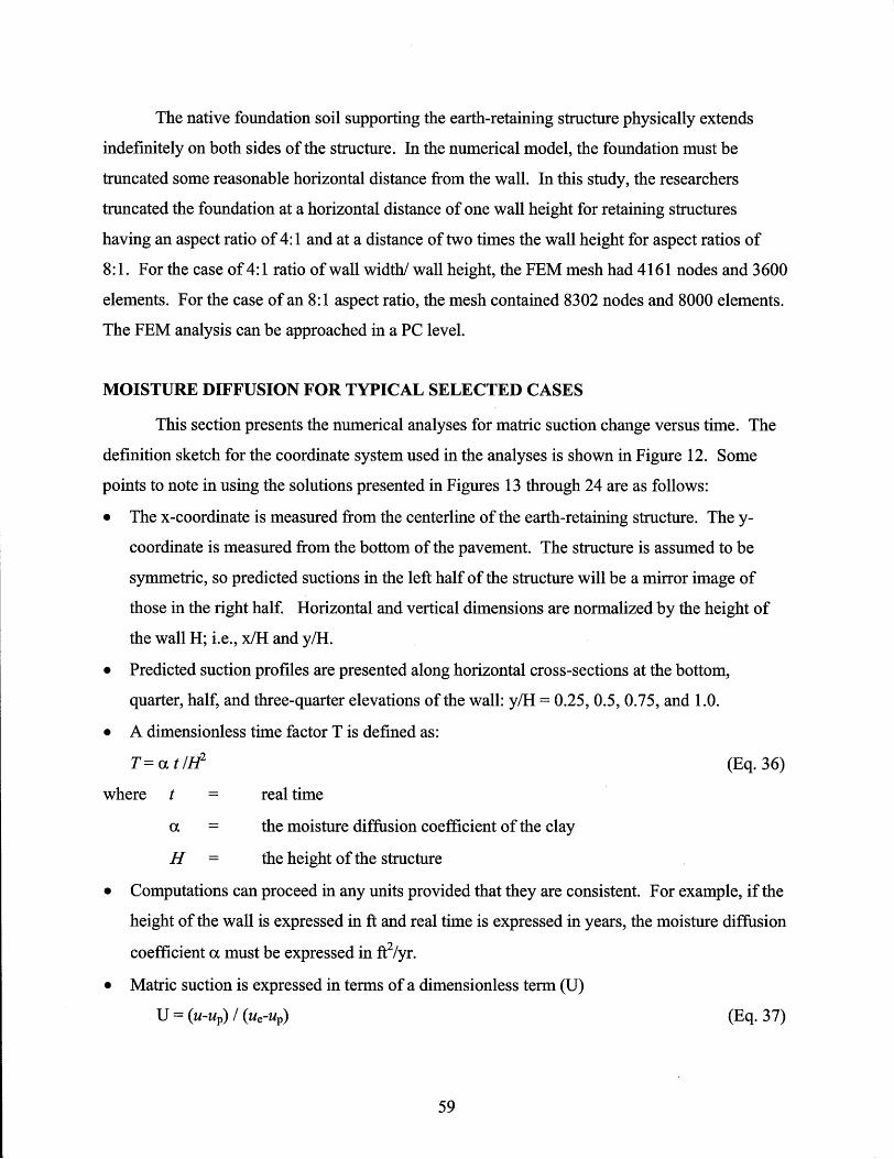
The native foundation soil supporting the earth-retaining structure physically extends
indefinitely on both sides of the structure. In the numerical model, the foundation must be
truncated some reasonable horizontal distance from the wall. In this study, the researchers
truncated the foundation at a horizontal distance of one wall height for retaining structures
having an aspect ratio of 4: 1 and at a distance of two times the wall height for aspect ratios of
8:1. For the case of 4:1 ratio of wall width! wall height, the FEM mesh had 4161 nodes and 3600
elements. For the case of an 8: 1 aspect ratio, the mesh contained 8302 nodes and 8000 elements.
The FEM analysis can be approached in a PC level.
MOISTURE DIFFUSION FOR TYPICAL SELECTED CASES
This section presents the numerical analyses for matric suction change versus time. The
definition sketch for the coordinate system used in the analyses is shown in Figure 12. Some
points to note in using the solutions presented in Figures 13 through 24 are as follows:
• The x-coordinate is measured from the centerline of the earth-retaining structure. The y
coordinate is measured from the bottom of the pavement. The structure is assumed to be
symmetric, so predicted suctions in the left half of the structure will be a mirror image of
those in the right half. Horizontal and vertical dimensions are normalized by the height of
the wall H; i.e., x/H and y/H.
• Predicted suction profiles are presented along horizontal cross-sections at the bottom,
quarter, half, and three-quarter elevations of the wall: y/H = 0.25, 0.5, 0.75, and 1.0.
• A dimensionless time factor T is defined as:
T= a t /H2
where t
a =
H =
real time
the moisture diffusion coefficient of the clay
the height of the structure
(Eq.36)
• Computations can proceed in any units provided that they are consistent. For example, if the
height of the wall is expressed in ft and real time is expressed in years, the moisture diffusion
coefficient a must be expressed in ft2/yr.
• Matric suction is expressed in terms of a dimensionless term (U)
U = (u-up) / (ue-up) (Eq.37)
59

where U = matric suction at time (t)
= the user-specified matric suction at the pavement-earthfill interface
Ue equilibrium matric suction at bottom of moisture-active zone
• The initial matric suction in the compacted earthfill is characterized by a parameter (Uo)
Uo = (uo-up) I (ue-up) (Eq. 38)
where uo is the initial matric suction in the compacted earthfill. Solutions are presented for (Uo)
values of 5,4, 3, 2, 1, and 0.5.
• Solutions are presented for retaining structure width-to-height ratios (W/H) of 4 (Figures 13
through 18) and 8 (Figures 19 through 24).
Centerline
Figure 12. Definition Sketch for Suction Predictions.
60
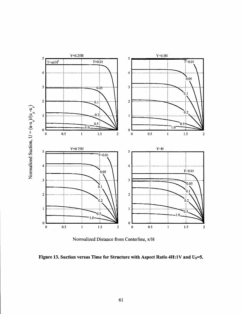
Y=0.25H 5~----~------~------~----~ T=O.Ol
: ::.:::::::::::::::I:::::::::::::::::::r·:::::::::::::::~:[::::::::.:::::
OL---~~~==~======~~ o 0.5 1.5 2
Y=0.75H
5~===+====~====~~-, T=O.Ol
4 ··················i .... ···············l .. ··········· : 1
3 ··················!··················r·········
. . . . 2
. . ··················1····················· ....... .
O~---------------------------o 0.5 1.5 2
Y=O.5H 5~ ____ ~ ____ ~ ____ -=~-----,
T=O.Ol
4 ··················[···················1················ .. ~ ............... .
! l 3 .................. i ................... J ....... ..
! : : : : : : : : : r-......... ~±: ~ ____ : I
2·············-<- .. ···· .. ·T ......... . 0.2
............ · .... j .......... ··· .. ·[· .......... :.:'1" ........... . 1.0--
OL-----L-----~~--~~~ o 0.5 1.5 2
Y=H 5~----~------~------T_----~
4 .................. ! ................... ! ............... ·····r·················· : : T=O.Ol
: : 2 ··················1················· .. 1 .... ······ t-__ ~i~_ !
. . ..... ~······ .. · .... · .... · .. 1 ........ ·-·· ........ ··· .. ·· .. ·r"·· .. ··· : :
O~--------------------------~ o 0.5 1.5 2
Normalized Distance from Centerline, xiH
Figure 13. Suction versus Time for Structure with Aspect Ratio 4H:l V and Uo=5.
61

Y=0.25H Y=O.5H 4~----~------~----~------~ 4~----~----~----~~--~ T=atlli T=O.Ol . . .
::: :::::: ::::::::::::1:::::::::::::::::::
1
:::::::::::::::::::1:::::: .. : :::::.:::
1 T=O.Ol 3.5 ................ · .. ~ ................... l ............. ······l·········· ..... .
3 . . ···················f···················]············· ...................... .
2.5
2 2
1.5 1.5
0.5 r----t-----i-__ 0.5 ~----~------~-
OL-----~----~~==~~ .. O~----~------~----~----~· o 0.5 1.5 2 o 0.5 1.5 2
Y=0.75H Y=H 4~----~------~----~-------
3.: ·:::.:: .. ·:.:::·:]· .. :::::.:.·:····.-1-·:.:··::.;:.:1 ..... : ... :::.:.::
2.5
2 .................. [" ...... . 2 .................. [" ....... .
1.5 1.5
0.5 t----i--......... ~:.:.:.:.. 0.5 ·················"1"·················T·····1.O
O~--------------------------- o o 0.5 1.5 2 o 0.5 1.5 2
Normalized Distance from Centerline, xlH
Figure 14. Suction versus Time for Structure with Aspect Ratio 4H:1V and Uo=4.
62

Y=0.25H
3~----~------~----~------~ T=O.Ql
2,: .:·:::::::::: .. :::i::: .. :: ... : .... ::.:I:::.: ... ~~~ ... :t .. ::::::: .. :::·::: 1.5
··················1····················r-············· ..
0.5 .................. j .................... :-.............. .
OL---~----~--~~==~~ o 0.5 1.5 2
Y=0.75H
3~====~====~====~---,
2.5 ···················:-··················r·········
, . 2 ' . ··················i···················1··········
~ ;
1.5 : ~
0.5 0.5 F .......... =..;.;~.:..;.;.;.;.;,;,;.;,:,;,:.:.::.:.:.::=:
1.0
T=O.Ol
O~------------~------~------o 0.5 1.5 2
Y=O.5H 3~ ____ ~ ____ ~ ____ ~~--~
2.5
2 I-----!----...;o~.
1.5
0.5
T=O.Ol
0.05 .. ····· .. · ... ,.
O~---~-----~------------~ o 0.5 1.5 2
Y=H 3r----.....,..---~--.....,.---..,
2.5 ···················!··················l·T~O~Oi"····l··· ............. .
2 .................. ; ................... :.......... 0.05! .. ···· .. ··· ..... .
: : : i
1.5
0.5 ········ .. ····· .. ·l .. ·· ...... · .... ····T·· ..
1 i O------~------~------------~ o 0.5 1.5 2
Normalized Distance from Centerline, xlH
Figure 15. Suction versus Time for Structure with Aspect Ratio 4H:IV and Uo=3.
63
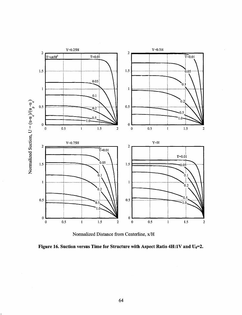
Y=O.25H Y=O.5H
2 ~----~------~------~----~ 2~ ____ ~ ____ ~ ____ ~=---~
T=O.Ol T=O.Ol
1.5 ··················i···················T ........... ~::5·1············ ... . 1.5 ··················1···················1-···················0.05······· ...
: : I
.-.., ::so.> I 0.5 ................................. 0.5 ::so..
'-' .......... .-.., 0.>
::s I
C- O 0 II 0 0.5 1.5 2 0 0.5 1.5 2 ~ d'" 0 .- Y=H ~ Y=0.75H <)
::s 2 2 r:n T=O.Ol ~
(I) T=O.Ol N .--~
S 1.5 .................................... -_ ................. 1.5
1 ~ 0 Z : i
, ,
.................. j ................... + ....... : : ! i : ! : 1
: 0.5 ' , 0.5 -_. __ ............... _- .......................... · ........ · ..... ·---.. ··· .. ·:-···.·-----··.· .. · ....... f-· .. · ..... -·
0 0 0 0.5 1.5 2 0 0.5 1.5 2
Nonnalized Distance from Centerline, xiH
Figure 16. Suction versus Time for Structure with Aspect Ratio 4H:IV and Uo=2.
64

Y=O.25H Y=O.5H
T=O.Ol T=O.Ol
::: .................. , ...... ·············r····::::::~.~~·:':::::::::::.::: .:: 0.8
0.6~ __ -..j... __
0.4 0.4
0.2
O~----~------~------~----~ O~----~------~----~------~ o 0.5 1.5 2 o 0.5 1.5 2
Y=O.75H Y=H
0.8 o 8 ..... a ....................... ~ ..... _______ • __ .... _ ..... ~. __ ...
. i .
0.6 0.6
0.4 t---...---~;,;,;.;,:,:,:= 0.4
0.2 .................. ; ................... + ................... j .... . ! i : j l ~
0.2 ··················l····················r·············· ..... j ............... .
~ 1 ~ i ~ ~ : : :
O~----~------~----~------~ O~----~------~------~----~ o 0.5 1.5 2 o 0.5 1.5 2
Normalized Distance from Centerline, x/H
Figure 17. Suction versus Time for Structure with Aspect Ratio 4H:1V and Uo=1.
65

Y=O.25H Y=O.5H 0.8 ..... --~~--......,.---....,.---.... 0.8 ..... ---...----...----...-----.
0.7 .... _ ... _ ................. --- ....................... , ..................................... -- .................. .
0.6 _ .. -.......... _ .. _ .. ---_ .................................................... - ....... ---- ..... ---- ..
0.5 T=O.OI ................. .
0.4 .................. ~ .................... ! ...... .
0.3 1---...... ---.-;..--....:..: 0.3 t----1-O';";';';';~
0.2 1---......;-........ -.;.;.:.:.:..: 0.2
0.1 0.1
o~------~----------------------~ 0 ..... ------...... ------..... ------..... ------.. o 0.5 1.5 2 o 0.5 1.5 2
Y=O.75H Y=H 0.8 0.8
0.7 0.7 , , ...................................... _ .............. _, ..... . , ,
0.6 0.6 ··················t···················t········· (i."i·f·· .............. .
0.5 0.5 , ,
0.4 0.4
0.3 0.3
: i 1.0 '
::::::.: : .. ::. : ... I ::. :.:. :.::.:::: :::r:::::::::::: ....... :: .... :::: ....... . 0.2 0.2
0.1 0.1
: : : : : :
_.- ...... __ .............. ~.- ----_ ... ---------1 .... ---- ... _ ...... -.- ... -.~- .... -........... _.
iii ··· .... ·············1-· .. · .. --------· .... ----:---·· .. ···· .. · .. · ......... ; .................. __ ...
l 1 1 : : .
0 0 0 0.5 1.5 2 0 0.5 1.5 2
Normalized Distance from Centerline, x/H
Figure 18. Suction versus Time for Structure with Aspect Ratio 4H:1V and Uo=O.5.
66

Y=O.25H Y=O.5H
i T=O.Ol
: ::::.:1:::::::. -::::.:::r:::::::I:::::::r:::~I:::::I:::.-: 4
3
2
0L-~--~~--~~~~==C3~ O~~--~--~--~--~--~--~~
o 0.5 1.5 2 2.5 3 3.5 4 o 0.5 1.5 2 2.5 3 3.5 4
Y=0.75H
4 ········t·········t······l·······r·····r··:r· 4 ·······t········l········1·········l······;t~~~·~l···· ... ")" ...... .
3
2 2
O~~--~--~--~--~--~--~-- O~~--~--~----------~----~ o 0.5 1.5 2 2.5 3 3.5 4 o 0.5 1.5 2 2.5 3 3.5 4
N onnalized Distance from Centerline, xlH
Figure 19. Suction versus Time for Structure with Aspect Ratio 8H:IV and Uo=5.
67

Y=O.25H 4~~--~--~--~--~~--~--~
i T=p.Ol i
2
1.5
0L-~ __ ~-L __ ~~-2~~~ o 0.5 1.5 2 2.5 3.5 4
Y=O.75H 4~~~==+=~~==~=r-'
i! i T=OOI i
3.5 ······~········+········i·······j······)········+:·····T··· .. .
3 ......... i .......... ~·········l········+······+········r········· ...... . 2.5
2 ········r········r·······r······r······-r·· 1.5
O~----------------~--------~ o 0.5 1.5 2 2.5 3 3.5 4
Y=O.5H 4~ .. --~--~~--~--.. ~~_,
i T=P.Ol ! 3.5 ........ ~ ...... , ... ~ .... ·····f··· ...... ; ......... ; .......... ~ ......... ~.... .
0.05 ! 3 ········_(··_·_··t······_·-t·······--l·_·····_·t-_····-t-···,_··, ..... .
2.: .: ..... l ....... ::i::::::.:.I.::.: ... :l. .... :: .. I .... : ... r:.:.: .. ' ...... :. 1.5
0.5 ........ ~ ..... , ... ~ .......... ! .......... ~ ......... ; ......... ~ ... .
O~~--~--~--~--~~--~~-o 0.5 1.5 2 2.5 3 3.5 4
Y=H 4~~--~--~--~--~--~--~~
3.: ·:::·::r .. ·:·:-r···::···].:.:::.:t:.:T:.:.:::t:.::.::::t.:.:·::. 2.5 ...... L ....... : ......... i ......... i ........ ~ .. o~t
2
1.5
······+········j·········i········+········[·········
Normalized Distance from Centerline, x/H
Figure 20. Suction versus Time for Structure with Aspect Ratio 8H:IV and Uo=4.
68

Y=0.25H 3 ~~~~--~--~--~--~--~~
i T=O.01 i
2.: :.:·:::1: ... ·.:·:,:::::::::1:: ... ::.:1::.:.:: .. 1:·::::::I~~ ... :,::·: .. --1.5
0.5
O~~--~--~--~--~--~--~~ o 0.5 1.5 2 2.5 3 3.5 4
Y=O.75H 3~~==~~==c=~==~:c-,
j T=OjOI
2.: .::: ... L:·:::r:"':':l:.::::::r .. :::T:.:.~r: "'1" ....
1.5
0.5 ········~········T·······r··
l j ~ : : :
O~------------~--~--------~ o 0.5 1.5 2 2.5 3 3.5 4
3~~ __ ~ __ ~Y_=0_.5~H __ ~ __ ~~~~
i T~.OI i !
2.5 --------r·····---l·····---l---------l---···---r-······ 2 ...... --;...---t---+--:-----_...:J
1.5 ········~·········l·········j········+······+······+· ........... .
0.5
O~~--~--~--~--~--------~ o 0.5 1.5 2 2.5 3 3.5 4
Y=H 3r-~--~--~--~--~--~--~~
2.5 ........ + ......... ~ ......... j ........ + ........ + ....... + ........ t· ...... · : : : : ! T=O.;QI i
2 QM · ...... ···· .... ···· ........ ·, .... · .... ·· .. · ...... · .... · .. o .. i .. ·
1.5
······ .. [·· .... ··T· ...... ·1' ...... ··r·· .. · • I • • I • I • •
O 5 . I I • I . · ...... ·!· .. ··· .. T .. · .. · .. r· ...... T· .. ·····! .... · .... r-[ ~ ~ ~ l ~
O~~---*------~--~--------~ o 0.5 1.5 2 2.5 3 3.5 4
Normalized Distance from Centerline, xIH
Figure 21. Suction versus Time for Structure with Aspect Ratio 8H:1 V and Uo=3.
69

2 ..... --,._....,.._.:,y_=0~.2=-5+H~"""P"""_~_.,....--. i T=O.OI
2~~ __ ~ __ y~=_0_.5_H~~ __ ~ __ ~~
i T=O.pl ! !
1.5 .. ··r···l····r······r····~.r·+· . 1.5
········:·········i·········j·········t·········!·········i·········,· ..... .
0.5 ········:·········;··········r·········,··············.Oi·········i·· ..
O~~-------------------------- O~~--~--~--~--~--~~~~ o 0.5 1.5 2 2.5 3 3.5 4 o 0.5 1.5 2 2.5 3 3.5 4
2F=~==~==y~==0=.7=5H==~==~==~-,
1.5 ··················;·········r········J···············
······i·····+······J:-········f·········:········T····.; ..... 0.5
0.5 ........ ! ......... j ......... t········.·········i·····I.O
O~~--~--~--~--~--~--~~ O~~--~--~--~--~--~--~~ o 0.5 1.5 2 2.5 3 3.5 4 o 0.5 1.5 2 2.5 3 3.5 4
Normalized Distance from Centerline, xlH
Figure 22. Suction versus Time for Structure with Aspect Ratio 8H:l V and Uo=2.
70

Y=O.25H
T=O.OI !
::: ........ l ......... r' ........ < .....•••. r ...... ~t·····i.':::::::l:::::.:'
0:1
0.4
O~~------~----------------~ o 0.5 1.5 2 2.5
Y=O.75H
0.8 ~----~---+--~--~
0.6
3 3.5
::: ::::::::':::::::::r::::::::1::::::::.:: ....... , ......... r·······,···
4
O~--------~----------------~ o 0.5 1.5 2 2.5 3 3.5 4
Y=0.5H
T=O.OI
0.8 ...• ~i ....... -i-...... . .... 7 ..• +. Q:Q5 ..... .
0.6 ........ ; ..... ····l·········j· ..... ···~··········~ ... ······f········
0.2 ........ , ......... : ......... : ......... , ......... ! .... .
O~~----------~------~--~~ o 0.5 1.5 2 2.5 3 3.5 4
Y=H
0.8
. . 0.6 ··· .... ·f···· .... ·l·· .. ·· .. ·l ...... · .. i .. ·· .. · .. ·r· ...... ·
::: ::::::::I:::::::::r::::::::+::::::·:+:::::::::I::::·::::1::·:::::·········
O~------------~------~--~~ o 0.5 1.5 2 2.5 3 3.5 4
Nonnalized Distance from Centerline, xlH
Figure 23. Suction versus Time for Structure with Aspect Ratio 8H:IV and Uo=l.
71
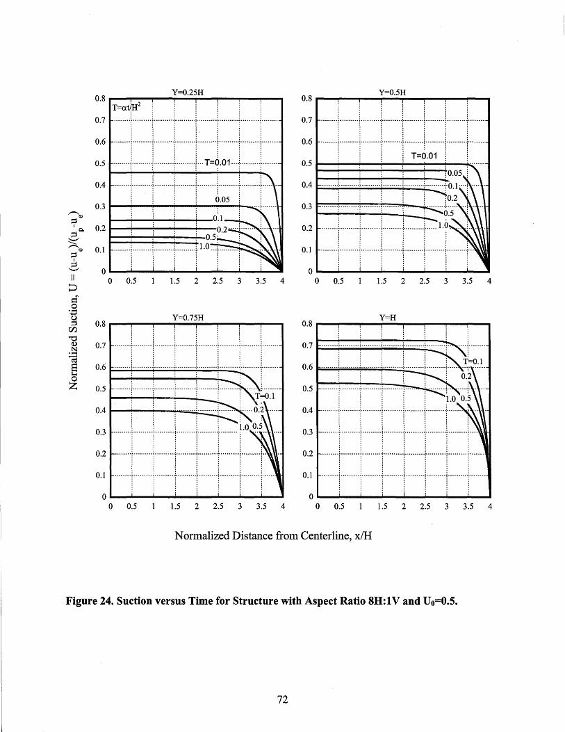
Y=0.25H 0.8 ........... - ...... -...,..-...,..-..... -.,...--,...--,.
Y=0.5H 0.8 ...... ....,-....,..-...,..-....... -,...-......,.-....,..-...
0.7
0.6 ···:····I:::::::·J·:·~~E·:·I::·:···::I::····· 0.5
0.4
;0.05
0.4 I-·-···-··-··'i-i···-··-··· .... ··i·-···-·.-... -io.~.-.. -... -... +j.-... -... -.. ~j··-···-··-.i..···1· 0 . 1 ···· r .... .
0.3 I--~.....;--;.-~-~-....;..---. 0.3
0.2 I----i---+-...... - ...... -- 0.2
0.1 0.1
O~------------~--~------------ O~--~~-~----------~~ o 0.5 1.5 2 2.5 3 3.5 4 o 0.5 1.5 2 2.5 3 3.5 4
Y=0.75H 0.8 ........... - ....... - ...... -~-....,..-...,..-...,..---.
Y=H 0.8 ........... ~ ....... - ...... - ...... -....,..-..,....-""I"'----.
....... r::.::.T::::::r:::::I····:-:-r:: ...... T::::::f:U
:
0.7
0.6
0.5
O. 7 t---'I'--i-----i~-.:-.......:. __
0.5
0.4
0.3 0.3
0.2 0.2
0.1 0.1
O~---~-~-~-~-~--~~ O~--~~-~-~-------~~ o 0.5 1.5 2 2.5 3 3.5 4 o 0.5 1.5 2 2.5 3 3.5 4
Normalized Distance from Centerline, xIH
Figure 24. Suction versus Time for Structure with Aspect Ratio 8H:IV and Uo=O.S.
72

USE OF SUCTION PREDICTION ANALYSES
This section presents an illustrative example of how the predicted suction versus time
relationships in Figures 12 through 23 may be used to compute soil strength changes over time.
The analyses will focus on computation of the shear strength in unconfined compression (Cue).
The example problem considers an earth-retaining structure 20 ft high with the width of
the compacted earthfill (see Figure 9) being 80 ft. The compacted clay has the following
properties:
~' 26 degrees
u 3xl0-5 cm2/sec
Yd 93lb/fe
w 24.2 percent
Gs 2.7
The reader is referred to Eq. 6 for empirically estimating the friction angle~' and to Eqs. 15 and
29 for estimating the diffusion coefficient u.
At a point located 30 ft from the centerline at the mid-depth of the structure, estimate the
strength of clay ( a) as-compacted, (b) after 20 years, and (c) after 40 years. Select suction
conditions typical of Central Texas, assume that the matric suction in the earthfill at the time of
placement is Uo = 3.5 pF, and assume wet conditions prevail beneath the pavement.
1. Dimensionless coordinates and times. To use the charts, coordinates and time must be
expressed in dimensionless terms. Coordinates are normalized by the height of the
structure (H). Therefore the dimensionless horizontal distance from the centerline is:
x / H = 30 ft / 20 ft = 1.5
Since the mid-depth is the point of interest, y = 0.5H.
The dimensionless time factor T is defined by Eq. 36. Since consistent units must be
used, the diffusion coefficient (u) must be converted to units offt2jyr. The conversion
will show that 3xl0-5 cm2/sec is equivalent to 1.0 ft2/yr. The dimensionless time factors
for the three times of interest are now as follows:
73

Real Time (years) Dimensionless Time, T = atlH2
0 0
20 0.05
40 0.10
2. Dimensionless Initial Suction, Vo. Predictions of suction require estimates of the suction
beneath the pavement (up), the equilibrium suction at the bottom of the moisture-active
zone in the sub-grade soil (ue), and the matric suction in the compacted soil (uo).
• Suction beneath pavement (up): The problem specified that wet conditions should be
assumed to prevail beneath the pavement. From the recommendation provided earlier in
this chapter, wet conditions would correspond to a matric suction up = 2 pF.
• Equilibrium suction (ue): From the recommendation provided earlier in this chapter, a
reasonable estimate of the equilibrium matric suction in Central Texas is Ue = 3.5 pF.
• Initial suction in earthfill (uo): The problem specified an initial matric suction in the
compacted earthfill Uo = 3.5 pF.
Based on these three suction values, the normalized suction value (Uo) for use in the
charts is:
Uo = (uo- up) I (ue- up) = (3.5 - 2) I (3.5 - 2) = 1
For a Uo value of 1.0 in a retaining structure having a 4H: 1 V aspect ratio, the appropriate
chart is found in Figure 17.
3. Suction versus Time from Charts. Entering Figure 17 for x I H = 1.5, and T = 0, 0.05, and
0.1, yields the dimensionless suction values shown in the table below. Dimensionless
suction from the chart is converted to real suction as follows:
F or use in strength calculations, the suction in pF must be converted to units of pressure.
Finally, the hydrostatic pressure due to the column of water above the point in question
should be added to the computed matric suction. This hydrostatic pressure correction
74

------------------------
should be made for any case in which the water in the soil voids is continuous; i.e., for
suction magnitudes less than 3.5 pF.
T U Suction, u Suction, hm Hydrostatic Corrected
(Figure 15) (PF) (pst) Correction Suction, hme
(pst) (pst)
0 1.0 3.5 -6470 620 -5850
0.05 0.80 3.20 -3240 620 -2620
0.10 0.57 2.86 -1480 620 -860
4. Shear Strength in Unconfined Compression from Suction. With the suctions estimated,
unconfined shear strength (Cue) calculations can proceed using Eq. 4. Chapter 2 presents
example strength calculations in great detail; therefore, all details are not repeated here.
The table below summarizes the main calculations.
Time Suction Gravimetric Saturation, Volumetric f Corrected Shear
(yrs) (PF) Moisture, w S(%) Moisture e Suction, Strength
(%) (%) hme (pst) Cue
(pst)
0 3.50 27.2 90.6 40.5 1.55 -5850 2870
20 3.20 27.9 93.0 41.6 1.75 -2620 1490
40 2.86 28.7 95.7 42.8 1.95 -860 560
75


CHAPTER 6: SUMMARY AND CONCLUSIONS
This research applies an analytical framework based on suction to characterize and
predict the performance of slopes and earth structures constructed of high-plasticity clays. A
generalized form of the Mohr-Coulomb strength criterion relates suction to strength. The
diffusion equation governs changes in suction with time and location. In general, this process is
non-linear for unsaturated soils. However, this research adopted an approach originally proposed
by Mitchell (4) by which appropriate transformation of the solution variable permits a linear
analysis. This linearization greatly simplifies the interpretation of test data to estimate the
required material parameters and simplifies the predictive framework.
The original moisture diffusion formulation required one material parameter, the
moisture diffusion coefficient (a). The original formulation was somewhat restrictive in that it
assumed a simple inverse relationship between matric suction and permeability. This research
generalized that formulation to allow the permeability to vary inversely with any power of
suction. This refinement introduces an additional material parameter, the exponent (n). The
tests performed by this research indicate that for shallow clay soils in the moisture-active zone,
Mitchell's initial assumption of the permeability exponent (n) equal to unity is reasonable.
However, for intact soils that have not been subjected to cracking, the permeability exponent (n)
may well be greater than unity. More investigations on intact soils are needed to explore this
issue. Laboratory tests performed in this research show a moisture diffusion coefficient (a) 0.8-
2.7 x 10⁻⁶ fr Imin for clays with liquid limits in the range of 56 to 66 and plasticity indices in the
range of34 to 44.
The stability and moisture diffusion analyses of 16 slope failures in Paris clays and 18
slope failures in Beaumont clays point to the following conclusions:
1. The slope failures are consistent with a condition of destabilizing hydraulic gradients. The
existence of such a condition provides the simplest plausible explanation as to why failures
would occur in slopes in which the angle of internal friction ($') of the soil is greater than the
slope angle (P).
2. Back-calculation of the apparent matric suction near the surface of the slopes at failure
indicate a fairly consistent value of about u(pF)=2.0 for high-plasticity clays. This "wet
limit" of suction represents a lower limit to which the magnitude of the matric suction will
77

decline when a free surface of soil is exposed to moisture without artificial disturbance of the
soil. The magnitude of the field capacity of suction is likely to be dependent on soil type,
with higher values associated with higher plasticity soils.
3. The observed failures are consistent with a phreatic surface located about 3 ft below the
surface of the slope. This phreatic surface is associated with a localized region of wetting
near the slope surface and is not, in general, associated with a regional groundwater table.
4. The time-dependent aspects of the slope failures can be explained in terms of (1) cracking on
the surface of the slopes, and (2) moisture entering the cracks and diffusing into the soil mass
until the magnitude of the suction and strength decline to a critical level.
5. The linearized moisture diffusion analyses for unsaturated soils provide useful first order
approximations to the rate of suction change and strength loss in the slope soils.
6. Estimates of the moisture diffusion coefficient (a) based on the drying test discussed in this
research appeared to be consistent with the time frame of the slope failures when cracking of
the soil mass is taken into consideration.
7. Although concrete riprap slope protection is not likely to be completely effective in
preventing moisture infiltration into a slope, it is likely to maintain the soil in a sufficiently
moist state to minimize desiccation cracking. By viewing the benefit of riprap in terms of its
ability to minimize cracking in the embankment rather than serving as a moisture barrier, one
may conclude that rock slope protection may be equally effective as concrete.
8. If concrete riprap slope protection is used, the top of the slope should be well drained to
prevent ponded water at the top of the slope from continuously feeding moisture into the
concrete-soil interface.
The moisture diffusion analysis framework used in this research was also extended to
typical TxDOT earth-retaining structures. Chapter 5 of this report presents a series of analyses of
changes in suction as a function of time and location. These suction predictions can provide a
basis for estimating strength degradation in earth-retaining structures over time.
78
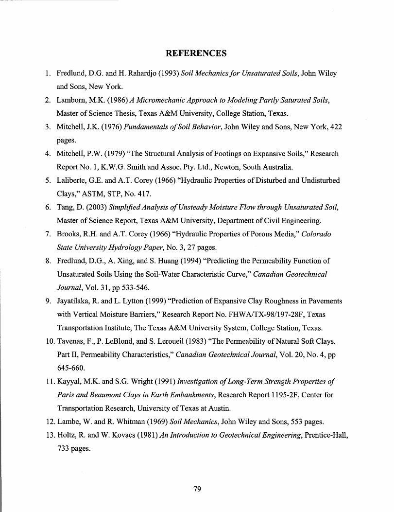
REFERENCES
1. Fredlund, D.G. and H. Rahardjo (1993) Soil Mechanicsfor Unsaturated Soils, John Wiley
and Sons, New York.
2. Lamborn, M.K. (1986) A Micromechanic Approach to Modeling Partly Saturated Soils,
Master of Science Thesis, Texas A&M University, College Station, Texas.
3. Mitchell, J.K. (1976) Fundamentals of Soil Behavior, John Wiley and Sons, New York, 422
pages.
4. Mitchell, P.W. (1979) "The Structural Analysis of Footings on Expansive Soils," Research
Report No.1, K.W.G. Smith and Assoc. Pty. Ltd., Newton, South Australia.
5. Laliberte, G.E. and A.T. Corey (1966) "Hydraulic Properties of Disturbed and Undisturbed
Clays," ASTM, STP, No. 417.
6. Tang, D. (2003) Simplified Analysis of Unsteady Moisture Flow through Unsaturated Soil,
Master of Science Report, Texas A&M University, Department of Civil Engineering.
7. Brooks, R.H. and A.T. Corey (1966) "Hydraulic Properties of Porous Media," Colorado
State University Hydrology Paper, No.3, 27 pages.
8. Fredlund, D.G., A. Xing, and S. Huang (1994) "Predicting the Permeability Function of
Unsaturated Soils Using the Soil-Water Characteristic Curve," Canadian Geotechnical
Journal, Vol. 31, pp 533-546.
9. Jayatilaka, R. and L. Lytton (1999) "Prediction of Expansive Clay Roughness in Pavements
with Vertical Moisture Barriers," Research Report No. FHW AlTX-98/197-28F, Texas
Transportation Institute, The Texas A&M University System, College Station, Texas.
10. Tavenas, F., P. LeBlond, and S. Leroueil (1983) "The Permeability of Natural Soft Clays.
Part II, Permeability Characteristics," Canadian Geotechnical Journal, Vol. 20, No.4, pp
645-660.
11. Kayyal, M.K. and S.G. Wright (1991) Investigation of Long-Term Strength Properties of
Paris and Beaumont Clays in Earth Embankments, Research Report 1195-2F, Center for
Transportation Research, University of Texas at Austin.
12. Lambe, W. and R. Whitman (1969) Soil Mechanics, John Wiley and Sons, 553 pages.
13. Holtz, R. and W. Kovacs (1981) An Introduction to Geotechnical Engineering, Prentice-Hall,
733 pages.
79
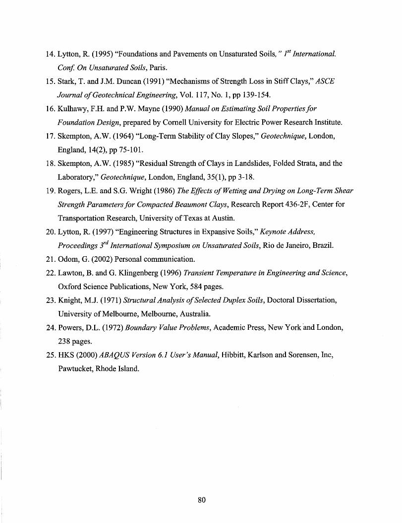
14. Lytton, R. (1995) "Foundations and Pavements on Unsaturated Soils, " 1st International.
Conf. On Unsaturated Soils, Paris.
15. Stark, T. and J.M. Duncan (1991) "Mechanisms of Strength Loss in Stiff Clays," ASCE
Journal o/Geotechnical Engineering, Vol. 117, No.1, pp 139-154.
16. Kulhawy, F.H. and P.W. Mayne (1990) Manual on Estimating Soil Properties/or
Foundation Design, prepared by Cornell University for Electric Power Research Institute.
17. Skempton, A.W. (1964) "Long-Term Stability of Clay Slopes," Geotechnique, London,
England, 14(2), pp 75-101.
18. Skempton, A.W. (1985) "Residual Strength of Clays in Landslides, Folded Strata, and the
Laboratory," Geotechnique, London, England, 35(1), pp 3-18.
19. Rogers, L.E. and S.G. Wright (1986) The Effects o/Wetting and Drying on Long-Term Shear
Strength Parameters/or Compacted Beaumont Clays, Research Report 436-2F, Center for
Transportation Research, University of Texas at Austin.
20. Lytton, R. (1997) "Engineering Structures in Expansive Soils," Keynote Address,
Proceedings 3rd International Symposium on Unsaturated Soils, Rio de Janeiro, Brazil.
21. Odom, G. (2002) Personal communication.
22. Lawton, B. and G. Klingenberg (1996) Transient Temperature in Engineering and Science,
Oxford Science Publications, New York, 584 pages.
23. Knight, M.J. (1971) Structural Analysis o/Selected Duplex Soils, Doctoral Dissertation,
University of Melbourne, Melbourne, Australia.
24. Powers, D.L. (1972) Boundary Value Problems, Academic Press, New York and London,
238 pages.
25. HKS (2000) ABAQUS Version 6.1 User's Manual, Hibbitt, Karlson and Sorensen, Inc,
Pawtucket, Rhode Island.
80

APPENDIX: MOISTURE DIFFUSION TEST SUMMARY
81


-LL 0.. ---c:: o :g ::J
en
-LL a. .......... c:: o :g ::J
en
5
4.5
4
3.5
4.8
4.7
4.6
4.5
4.4
4.3
4.2
Test 1 Psychrometer 5 Length = 29.21cm x=21.59cm uo=3.39pF
u =5.64pF a
I~--------------~: I I ••••••••••••••• J • • • • • • •• • • • • • • • • ... • • • • • • • • • • • • •• • -1- •••••••••••••••
I I I I I I I I I
I I I I
I I
I I I ............... ~ ................. ~ ................ : .. ............. .
103
a = 0.0046cm2/min
(7.7 10-5 cm2/sec)
Time (minutes)
Test 1 Psychrometer 6 Length = 29.21cm x=25.40cm uo=4.20pF
u =5.64pF a
• I
I I I I . . . . . . . .. _ .. ~ .................... . I
......•.... t·· ..... -_ ........... . ~--------------~ I
I I
I
I I ••••••••••••••••••••• ill • • • • • •• • ••••••••••••• _,8 ••••••••••••••••••••• . :. . ~--: ----------....,
I I
c.:.:' '.=,.:' ',:.:.' '.::.:.' ''='':'-._. ......~. l' ................ . a = 0.0018cm2/min
(3.0 10-5 cm2/sec) I I I I
Time (minutes)
83

4.1
4
3.9 -LL a. 3.8 .......... c 0
:t:i 3.7 (.)
:::J (j)
3.6
3.S
S
4.8
4.6
-LL a. 4.4 .......... c 0 :0 4.2 :::J (j)
4
3.8
Test 2 Psychrometer S Length = 24.13cm x=17.78cm
I I I I I · ~ ................................ . I
uo=3.4SpF
u =S.83pF a
I I . . . . . . .. . ... . .. . .. . . .. . .. .... ... .. I I I I I I I . ,. . .. . . . ... .. . . . . . . ... ... ... . ....
~--------------~, I I I I I
•••••••••••••••••••••••••••••••••• 1. • • • • • • • • ••• • ••• • • • • •• •• • •••••••
a = O.0024cm2/min I I
(4.0 10-5 cm2/sec) ······i································ : . I ••••••••••••••••••••••••••••••••• r ••••••••••• . : I
103
Time (minutes)
Test 2 Psychrometer 6 Length = 24.13cm x=21.S9cm uo=3.7SpF
u =S.83pF a
I I I I I I
... • • • • • • • •• • • •• ..81 8 •••••••••••••••
: I
I I I I I • f . . . . • . • ... . ..... : .•••.....•••.... : ~ : : .: · ~ ................ ~ .............. .
I~--------------~, I
: • ! I I
I ~ : •••••••••••••••• ~ ••••••••••••••••• 1 ................................. .
: .: : : • I I I I I I I I . . . . .. . . . . . . . .. . . . . . . . . . .. . . . . . .. . ................ : ............... . I I .: ~--~I------~ I I
I I 2 ••••...•.•..... ~ .......•......•• t ...... a = 0.0030cm Imin ~~ ____ ~' ___ I
l (S.O 10-5 cm2/sec)
103
Time (minutes)
84

G:' a. -.... c o ~ :::J (j)
-I.L. a. ---c o
:;:; () :::J
(j)
5
4.5
4
3.5
3
5
4.5
4
3.5
, , , I , , , ,
Test 3 Psychrometer 4 Length = 22.22cm x=13.34cm . ...... . . . .. .... ... . ..... ... ... . .. . uo=2.60pF
u =5.BOpF a
, , , ,
, , , , , , , a = 0.0024cm2/min .......... -i- .................. ..
,
(4.0 10-5 cm2/sec) j • . : ..................... ~ ..................... . , , , , , ,
Time (minutes)
Test 3 Psychrometer 5 Length = 22.22cm x=15.51cm
, , , I , , , , , ,
uo=3.20pF I , .," ............... , ............. .
u =5.BOpF a
I I I , I I
I~------~------~: I I I ,
···············i·················~·················:·· ............ . I , ,
a = O.00090cm2/min
(1.5 10-5 cm2/sec)
.:~-----.......... --~ I ,
103
Time (minutes)
85
I I I I I I I , I I

-u.. a. -..-c: o :g ::J en
-u.. a. -..-c: o :g ::J en
4.8
4.6
4.4
4.2
4
I I I I
Test 3 Psychrometer 6 Length = 22.22cm x=19.69cm ............. , .................... .
I
uo=3.90pF
u =5.80pF I a ..............................
a = 0.0012cm2/min
(2.0 10-5 cm2/sec) I
: . • ...•................ ~ ....................... ~ .. : I
I I
3.8 101
5
Time (minutes)
Test 4 Psychrometer 4 Length = 20.96cm x=12.07cm uo=3.60pF
I I I I I I I I
4.5 u =5.91pF ••••••••••• •• 1. • • • • • •• • • • • • • • •• • •••
4
3.5 102
a
a = 0.0014cm2/min
(2.3 10-5 cm2/sec)
• I I
: . I
Time (minutes)
86

-LL. c.. ---c 0
:;::; 0 ~
en
-LL. 0----c 0 :g ~
en
4.15
4.1
4.05
4
3.95
3.9
3.85
3.8
Test 4 Psychrometer 5 Length = 20.96cm x=15.24cm uo=3.80pF
u =5.91pF a
I I I I .: ..................................... .. I I I I I
I I I I • r • • • • • • • • • • • • • •• • • • • • •• • • • • • • • .. I I I
J----------------~: .................................. ,... . .. . . .. . . . .. .. . ... .... . .. .... ... . ...... ~------------~:
I I • a = O.0013cm2/min
(2.2 1 0.5 cm2/sec)
-:- .............. ~..... ....... . ....... .. I I I I I
.. .. .... .. .. .. .. .. ...... ...... .. .. .... .... .. .. .. .. .. .. .. .. .. .. .... .. .......... ..
3.75 102 103
5
4.8
4.6
4.4
4.2
4
Time (minutes)
Test 4 Psychrometer 6 Length = 20.96cm x=18.42cm uo=3.80pF
u =5.91 pF a
a = 0.0022cm2/min
(3.7 10.5 cm2/sec)
I I I I I •..•••.•••. • -I- ...•..•.•..•.•.••••• I
I
3 8 .~.................. I • 'I0&0&0&0...._----, •••••••••• : •••••••••••••••••••••
Time (minutes)
87
I I I I

-LL C. -c: a :n ::l
CI)
-LL C. -c: a :n ::l
CI)
4.6 Test 5 Psychrometer 6
4.5 L = 20.32 cm
I I I I I ••.••.. -I- ................... .
x = 17.78 cm I I I I I I u = 5.74pF
a
uo = 3.95pF 4.4 ........ f ............ ...... ..
4.3 h = 0.54cm-1
4.2
4.1
4
3.9 10
4.4
4.3
4.2
4.1
4
3.9
3.8
3.7
e
a = 0.0010 cm2/min
(1.7 10-5 cm2/sec) ..................... , ....................... ~ .. . ................ . .: I
100 1000 10000
Time (minutes)
Test 6 Psychrometer 5 Length = 19.05cm x=13.72cm
............ -I- .................... .
uo=3.75pF
u =6.00pF a
I I I I I I I ••••••••••••• r ••••••••••••••••••••• I I I I I
a = O.0019cm2/min
(3.2 10-5 cm2/sec) : ..
I I I I
•••••••••••••••• ':&. ••• ~ ••••••••••••••••••••••• ~ •••••••••••••••••••• ... I I
I I I I
10 100 1000 10000
Time (minutes)
88

-LL 0. ---c o ts :::J
en
-LL 0. ---c 0 ts :::J
en
4.7
4.6
4.5
4.4
4.3
4.2
4.1
4
4.1
4
3.9
3.8
3.7
3.6
3.5
3.4
3.3
Test 6 Psych rometer 6 Length = 19.05cm x=16.51cm u =4.10pF
o u =6.00pF
a
I I I ............. ,. .. . . . . . . . . . . . . . . .. .. I I I I I I ••••••••••••• t • • • • • • • •• • • • • •• • ••••
I~--------------~ I
10
10
a = 0.00076cm2/min
(1.3 1 O-~ cm2/sec) I I I I ..................... , .................... .
I I I
100 1000
Time (minutes)
10000
Test 7 Psychrometer 5 Length = 21.59cm x=15.88cm
............ ~ .................... . I I I I I I
u =3.40pF ••••••••••• • 818 • • • • • •• • • • • • • • • • • •• •
o I I I I I u =5.62pF
a ............. ~ . . . . . . . . . . .. . . . . . . . I I I I
.................... .. : ....................... ! ............. ~ .... . I I I I
a = 0.0025cm2/min
(4.2 10-5 cm2/sec) I
~--------~------~.~ ......... : ••••.....••....•••...
100
I I I
1000
Time (minutes)
89
10000

-u. c. -c 0
t5 ::J
en
---u. c. ---c o t5 ::J en
4.B
4.6
4.4
4.2
4
3.B
3.6
4.4
4.2
4
3.B
3.6
3.4
3.2
3
10
I
Test 7 Psychrometer 6 Length = 21 .S9cm x=18.Bcm
............. ~ . .. . .. ... . .. . .. . .. ..
uo=3.7pF
u =S.62pF a
I I I I I I I ............ t· ............ . I
I I •••••••••••••••••••• •• 1 ••••••••••••••••••••••• .J. • • • • • ••• • ••••••••••
I I I I
I I I I I I
a = 0.0028cm2/min
(4.7 10-5 cm2/sec) ..... .. ,.. .. -:-. .. . ............... .
I I ..................... ~ .................. .
• I I I
100 1000
Time (minutes)
10000
Test 9 Psychrometer S Length = 22.B6cm x=16.76cm
. ~ . .. . . .. . . . . . . .. . .. . .. . . . . . . . ... .
uo=3.10pF
u =S.93pF a
a = 0.00SOcm2/min
(B.3 10-5 cm2/sec)
I I
I I I I
• . ... . .. . . .. . ................... . • ••••••••••••••••••••••••••••••••• T ••
100 1000
Time (minutes)
10000
90


![Tensile Strength of Compacted Clays · 2015-09-16 · 6 0 50 100 150 200 250 300 tensile force [kp A] 0 200 400 600 800 time [sec] upper part upper sample middle and lower sample](https://img.dokumen.tips/doc/110x75/5e627554f52ec33aa75f2221/tensile-strength-of-compacted-2015-09-16-6-0-50-100-150-200-250-300-tensile-force.jpg)