Long-Term Effects of Teacher Performance Pay:

Experimental Evidence from India

Karthik Muralidharan†

10 April 2012* Abstract: We present results from a five-year long randomized evaluation of group and individual teacher performance pay programs implemented across a large representative sample of government-run rural primary schools in the Indian state of Andhra Pradesh. We find consistently positive and significant impacts of the individual teacher incentive program on student learning outcomes across all durations of program exposure. Students who completed their full five years of primary school under the program performed significantly better than those in control schools by 0.54 and 0.35 standard deviations in math and language tests respectively. These students also scored 0.52 and 0.3 standard deviations higher in science and social studies tests even though there were no incentives on these subjects. The group teacher incentive program also had positive (and mostly significant) effects on student test scores, but the effect sizes were always smaller than that of the individual incentive program, and were not significant at the end of primary school for the cohort exposed to the program for five years. These results suggest that reforming the compensation structure of public sector employees could play an important role in enhancing the capacity of governments in developing countries to provide more effective services. JEL Classification: C93, I21, M52, O15

Keywords: teacher performance pay, teacher incentives, education, education policy, field experiments, public sector labor markets, compensation, India

† UC San Diego, NBER, BREAD, and J-PAL; E-mail: kamurali@ucsd.edu * I am especially grateful to Venkatesh Sundararaman for the long-term collaboration that has enabled this paper and to the World Bank for the long-term support that has enabled the research program that this paper is based on. I thank Jim Andreoni, Prashant Bharadwaj, Julie Cullen, Jishnu Das, Gordon Dahl, and Andres Santos for comments. This paper is based on a project known as the Andhra Pradesh Randomized Evaluation Study (AP RESt), which is a partnership between the Government of Andhra Pradesh, the Azim Premji Foundation, and the World Bank. Financial assistance for the project has been provided by the Government of Andhra Pradesh, the UK Department for International Development (DFID), the Azim Premji Foundation, the Spanish Impact Evaluation Fund (SIEF), and the World Bank. We thank Dileep Ranjekar, Amit Dar, and officials of the Department of School Education in Andhra Pradesh for their continuous support and long-term vision for this research. We are especially grateful to DD Karopady, M Srinivasa Rao, Sripada Ramamurthy, and staff of the Azim Premji Foundation for their leadership and meticulous work in implementing this project. Vinayak Alladi, Jayash Paudel, and Ketki Sheth provided outstanding research assistance.

- 1 -

1. Introduction

Improving governance in developing countries requires improved policy making as well as

enhancements in the capacity of governments to effectively implement policies. This point is

reflected in a recent theoretical literature that has highlighted the centrality of investments in

state capacity in long-term growth and development (Besley and Persson 2009, 2010), as well as

a parallel empirical literature that has pointed out the extent to which developing countries find it

challenging to ensure even basic levels of service delivery such as regular attendance of teachers

and health care workers in rural communities (World Bank 2003; Chaudhury et al. 2006;

Muralidharan et al. 2012).1

Since the effort exerted by public sector employees is a key determinant of state

effectiveness, a natural set of policy options to enhance state capacity would be to consider

linking public sector worker compensation to measures of performance. However, high-

powered incentives have typically not been used for public sector workers for several reasons

including concerns of multi-tasking (Holmstrom and Milgrom 1991) and multiple principals

(Dixit 2002); concerns of implementation (Murnane and Cohen 1986); greater unionization of

public sector workers and the opposition of unions to differentiated pay schemes based on

performance (Ehrenberg and Schwarz 1986; Gregory and Borland 1999); and perhaps also

because decision-makers in public bureaucracies are typically not residual claimants of improved

productive efficiency (Bandiera, Prat, and Valletti 2009). At the same time, an increasing

fraction of private sector jobs now link some component of employee pay to performance

(Lemieux, Macleod, and Parent 2009), prompting increasing interest among policy makers in

using performance-linked pay as a way of improving public sector productivity.

This trend is particularly visible in education, where the idea of linking a component of

teacher compensation to measures of student performance or gains has received growing

attention from policy makers, and several countries as well as states in the US have attempted to

implement reforms to teacher compensation structure to do this.2 Since teachers typically

1 Indeed, the large disconnect between policy formation and implementation in countries like India has led to the coining of the term ‘flailing state’ to describe countries with a weak capacity for effective policy implementation (Pritchett 2009). 2 Countries that have attempted teacher performance pay programs include Australia, Israel, Mexico, the United Kingdom and Chile (which has a fully scaled up national teacher performance pay program called SNED). In the US, states that have implemented state-wide programs to link teacher pay to measures of student achievement and/or gains include Colorado, Florida, Michigan, Minnesota, Texas, and Tennessee. In addition, the US Federal

- 2 -

comprise one of the largest groups of public-sector workers in most countries, understanding the

impact of performance-based pay in education is especially relevant to the broader question of

the role of compensation reforms in improving public sector productivity.

In this paper, we contribute towards this understanding with results from a five-year long

randomized evaluation of group and individual teacher performance pay programs implemented

across a large representative sample of government-run rural primary schools in the Indian state

of Andhra Pradesh (AP). Results at the end of two years of this experiment were presented in

Muralidharan and Sundararaman (2011) and half of the schools originally assigned to each of the

group and individual incentive programs (50 out of 100) were chosen by lottery to continue

being eligible for the performance-linked bonuses for a total of five years. Since primary school

in AP consists of five grades (1-5), the five-year long experiment allows us to measure the

impact of these programs on a critical outcome for education in developing countries – the

learning levels for a cohort of students at the end of their entire primary school education.

There are three main results in this paper. First, the individual teacher performance pay

program had a large and significant impact on student learning outcomes over all durations of

student exposure to the program. Students who had completed their entire five years of primary

school education under the program scored 0.54 and 0.35 standard deviations (SD) higher than

those in control schools in math and language tests respectively. These are large effects

corresponding to approximately 20 and 14 percentile point improvements at the median of a

normal distribution, and are larger than the effects found in most other education interventions in

developing countries (see Dhaliwal et al. 2011).

Second, the results suggest that these test score gains represent genuine additions to human

capital as opposed to reflecting only ‘teaching to the test’. Students in individual teacher

incentive schools score significantly better on both non-repeat as well as repeat questions; on

both multiple-choice and free-response questions; and on questions designed to test conceptual

understanding as well as questions that could be answered through rote learning. Most

importantly, these students also perform significantly better on subjects for which there were no

incentives – scoring 0.52 SD and 0.30 SD higher than students in control schools on tests in

science and social studies (though the bonuses were paid only for gains in math and language).

Government has encouraged states to adopt performance-linked pay for teachers through the “Race to the Top” fund that provides states that innovate in these areas with additional funding.

- 3 -

There was also no differential attrition of students across treatment and control groups and no

evidence to suggest any adverse consequences of the programs.

Third, we find that individual teacher incentives significantly outperform group teacher

incentives over the longer time horizon though they were equally effective in the first year of the

experiment (the point estimates suggest that the individual incentive program was more effective

than the group incentive program at every time horizon in both math and language). Students in

group incentive schools score better than those in control schools over most durations of

exposure, but these are not always significant and students who complete five years of primary

school under the program do not score significantly higher than those in control schools.

We measure changes in teacher behavior and the results suggest that the main mechanism for

the improved outcomes in incentive schools is not reduced teacher absence, but increased

teaching activity conditional on presence. We also measure household responses to the program

– for the cohort that was exposed to five years of the program, at the end of five years – and find

that there is no significant difference across treatment and control groups in either household

spending on education or on time spent studying at home, suggesting that the estimated effects

are unlikely to be confounded by differential household responses across treatment and control

groups over time. Finally, our estimates suggest that the individual teacher bonus program was

15-20 times more cost effective at raising test scores than the default ‘education quality

improvement’ policy of the Government of India, which is reducing class size from 40 to 30

students per teacher (Govt. of India, 2009).

The central questions in the literature on teacher performance pay to date have been whether

teacher performance pay based on test scores can improve student achievement, and whether

there are negative consequences of teacher incentives based on student test scores? On the first

question, two recent sets of experimental studies in the US have found no impact of teacher

incentive programs on student achievement (see Fryer 2011, and Goodman and Turner 2010 for

evidence based on an experiment in New York City, and Springer et al 2010 for evidence based

on an experiment in Tennessee). However, other well-identified studies in developing countries

have found positive effects of teacher incentives on student test scores (see Lavy 2002 and 2009

in Israel; Glewwe et al. 2010 in Kenya; and Muralidharan and Sundararaman 2011 in India).

Also, Rau and Contreras (2011) conduct a non-experimental evaluation of a nationally scaled up

teacher incentive program in Chile (called SNED) and find positive effects on student learning.

- 4 -

On the second question, there is a large literature showing strategic behavior on the part of

teachers in response to features of incentive programs, which may have led to unintended (and

sometimes negative) consequences. Examples include 'teaching to the test' and neglecting

higher-order skills (Koretz 2002, 2008), manipulating performance by short-term strategies like

boosting the caloric content of meals on the day of the test (Figlio and Winicki, 2005), excluding

weak students from testing (Jacob, 2005), re-classifying more students as special needs to alter

the test-taking population (Cullen and Reback 2006), focusing only on some students in response

to "threshold effects" embodied in the structure of the incentives (Neal and Schanzenbach, 2010)

or even outright cheating (Jacob and Levitt, 2003).

The literature on both of these questions highlight the importance of not just evaluating

teacher incentive programs that are designed by administrators, but of using economic theory to

design systems of teacher performance pay that are likely to induce higher effort from teachers

towards improving human capital and less likely to be susceptible to gaming (see Neal 2011).

The program analyzed in this paper takes incentive theory seriously and the incentives are

designed to reward gains at all points in the student achievement distribution, and to penalize

attempts to strategically alter the test-taking population. The study design also allows us to test

for a wide range of possible negative outcomes, and to carefully examine whether increases in

test scores are likely to represent increases in human capital. This experiment is also the first one

that studies both group and individual teacher incentives in the same context and time period.3

Finally, to our knowledge, five years is the longest time horizon over which an experimental

evaluation of a teacher performance pay program has been carried out and this is the first paper

that is able to study the impact on a cohort of students of completing their entire primary

education under a system of teacher performance pay.

While set in the context of schools and teachers, this paper also contributes to the broader

literature on performance pay in organizations in general and public organizations in particular.4

There has been a recent increase in compensation experiments in firms (see Bandiera et al. 2011

3 There is a vast theoretical literature on optimal incentive design in teams (Holmstrom 1982 and Itoh 1992 provide a good starting point). Kandel and Lazear (1992) show how peer pressure can sustain first best effort in group incentive situations. Hamilton, Nickerson, and Owan (2003) present empirical evidence showing that group incentives for workers improved productivity relative to individual incentives (over the 2 year study period). Lavy (2002 and 2009) studies group and individual teacher incentives in Israel but over different time periods and with different non-experimental identification strategies. 4 See Lazear and Oyer (2009) for a recent review of the literature in personnel economics (which includes a detailed discussion of worker incentives), and Dixit (2002) for a discussion of these themes applied to public organizations.

- 5 -

for a review), but these are typically short-term studies (often lasting just a few months). 5 The

results in this paper are based (to our knowledge) on the longest running experimental evaluation

of group and individual-level performance pay in any sector. More broadly, in the absence of

high-powered incentives for public sector workers, the literature on determinants of governance

quality has highlighted the role of bureaucratic culture (Wilson 1989), professionalism in the

bureaucracy (Evans and Rauch 1999) and selection of workers who are motivated by the public

interest (Besley and Ghatak 2005). A parallel literature has looked at the role of compensation

levels on the characteristics of workers who join the public sector and usually finds that

improving levels of pay helps attract more educated workers, but this literature has typically not

looked at whether this leads to improved outcomes, or if across the board pay increases are cost

effective ways of doing so (Dolton 2006; Dal Bo, Finan, and Rossi 2011). Our results highlight

the potential for well-designed changes in compensation structure (as opposed to levels) to

improve public sector productivity in a cost-effective way.

The rest of this paper is organized as follows: section 2 describes the experimental design;

section 3 discusses data and attrition; section 4 presents the main results of the paper; section 5

discusses changes in teacher and household behavior in response to the programs, and section 6

concludes.

2. Experimental Design

2.1 Theoretical Considerations

Standard agency theory suggests that having employee compensation depend on measures of

output will increase the marginal return to effort and therefore increase effort and output.

However, two broad sets of concerns have been raised about introducing performance-linked pay

for teachers. First, there is the possibility that external incentives can crowd out intrinsic

motivation and reduce effort – especially in jobs such as teaching that attract intrinsically

motivated workers (Deci and Ryan 1985; Fehr and Falk 2002). The second set of concerns is

based on multi-tasking theory which cautions that rewarding agents on measurable aspects of

their efforts may divert effort away from non-measured outputs, leading to inferior outcomes

5 One limitation of short-term compensation experiments is the inter-temporal substitutability of leisure, which may cause the impact of a temporary change in wage structure to be different from the impact of a long-term change.

- 6 -

relative to a scenario with no performance-pay at all (Holmstrom and Milgrom 1991; Baker

1992).

Muralidharan and Sundararaman (2009) discuss the first concern and suggest that a

transparently administered performance-linked pay program for teachers may actually increase

intrinsic motivation in contexts (like India) where there is no differentiation of career prospects

based on effort. Muralidharan and Sundararaman (2011) discuss the second concern in detail

and show that the social costs of the potential diversion of teacher effort from ‘curricular best

practice’ to ‘maximizing test scores’ may be limited in contexts like India where (a) ‘best

practice teaching’ is typically not very different from teaching to maximize scores on high-stakes

tests (which are ubiquitous in India), and (b) norms of teacher effort in the public sector are quite

low (which is also true in India, with 25% of public school teachers being absent on any given

day – see Kremer et al. 2005).

So, it is possible that linking teacher pay to improvements in student test scores will not only

increase test scores, but also increase underlying human capital of students, especially in

contexts such as India. Whether or not this is true is an empirical question and is the focus of

our research design and empirical analysis.

2.2 Background

The details of the experimental design (sampling, randomization, incentive program design,

and data collected) are discussed in detail in Muralidharan and Sundararaman (2011) – hereafter

referred to as MS 2011, and are only summarized briefly here. The original experiment was

conducted across a representative sample of 300 government-run primary schools in the Indian

state of Andhra Pradesh (AP), with 100 schools each being randomly assigned to an “individual

teacher incentive program”, a “group teacher incentive program”, and a control group. The

study universe was spread across 5 districts, with 10 mandals (sub-districts) being randomly

sampled from each of the 5 study districts, and 6 schools being randomly sampled from each of

the 50 mandals. The randomization was stratified at the mandal level and so 2 of the 6 schools in

each mandal were assigned to each treatment and to the control group.

The bonus formula provided teachers with Rs. 500 for every percentage point of mean

improvement in test scores of their students. The teachers in group incentive (GI) schools

received the same bonus based on average school-level improvement in test scores, while the

bonus for teachers in individual incentive (II) schools was based on the average test score

- 7 -

improvement of students taught by the specific teacher. Teachers/schools with negative

improvements did not get a bonus (there was no negative bonus). The main features of the

incentive design were: (i) the bonus was based on a linear piece-rate – which provided a

continuous incentive for effort, since a larger test score gain led to a larger bonus; (ii) there were

limited threshold effects, since all students contributed to the bonus calculation; (iii) the

incentive amounts were not large, with the expected value of the bonus being around 3% of

annual teacher pay. See MS 2011 for further details of the incentive formula and the rationale

for each of the design features.

2.3 Changes in Experimental Design

The design details were unchanged for the first two years of the experiment (up to the point

reported in MS 2011), and the experiment was initially only expected to last for two years.

Renewed funding for the project allowed the experiment to continue for a third year, at which

point, a small change was made to the bonus formula. In the first two years, student gains were

calculated using their previous test score as a baseline. While this was an intuitive way of

communicating the details of the system to teachers, it had an important limitation. Since there

is substantial mean reversion in student scores, the formula unfairly penalized teachers who had

an incoming cohort of high-scoring students and rewarded those who had an incoming cohort of

low-scoring students. Once we had two years of data in control schools, we were able to

calculate a ‘predicted’ score for each student using lagged scores and use this predicted score

(predicted using only the control schools) as the ‘target’ for each student in the incentive school

to cross to be eligible for the bonus. The final bonus was calculated at the student level and then

aggregated across students for the teacher/school. The formula used to calculate the bonus at the

individual student level was:

Student level bonus = Rs. 20 × (Actual Score – Target Score).6 (1)

In cases where the actual score was below the target score, a student could contribute a

‘negative amount’ to the teachers’ bonus, but this was capped at -5% or – Rs. 100 (even if the

actual score was more than 5% below the target score). Cases of drop-outs (or non-test taking of

students who should have taken the test) were automatically assigned a score of -5% and

6 The scores are defined in terms of “% age score on the test”. A typical teacher taught around 25 students and so a bonus of Rs. 500 per percentage point improvement in average scores in the class was equivalent to a bonus of Rs. 20 per student per percentage point improvement in student-level scores. Thus, the change in formula was not meant to change the expected amount of bonuses paid, but rather to reduce the role of mean reversion in the award of bonuses.

- 8 -

contributed to a reduction of the bonus by Rs. 100. Thus, a student could never hurt a

teacher/school’s bonus more than by not taking the test, and it was therefore not possible to

increase the ‘average’ score by having weak students drop out. While it was possible for an

individual student to contribute a negative amount to a teacher’s bonus, the final bonus received

by teachers was zero and not negative in cases where the total bonus was negative after

aggregating (1) across all the students taught by the teacher/school.

At the end of the third year, uncertainty regarding funding required a reduction in the sample

size of the project. It was decided that it would be valuable to continue the experiment for at

least a subset of the original treatment group for five years, to study the impact of the programs

on a cohort of students who had completed their entire primary school education (grades 1-5)

under the teacher incentive programs. Hence, both group and individual incentive programs

were continued in 50 of the 100 schools where they started, and discontinued in the other 50.

The selection of schools to continue or discontinue was done by lottery stratified at the mandal

level and so each of the 50 mandals in the project had 1 school that continued with each

treatment for 5 years, 1 school that had each treatment for 3 years and was then discontinued

from the treatment, and 2 schools that served as control schools throughout the 5 years of the

project (see Figure 1). Since the focus of this paper is on the effects of extended exposure to the

teacher incentive treatments, most of the analysis will be based on the schools that continued

with the treatments for 5 years (when treatment effects over 3 years or more are being

considered).

2.4 Cohort and Grade Composition of Students in Estimation Sample

Primary school in AP covers grades 1 through 5 and the project lasted 5 years, which meant

that a total of 9 cohorts of students spent some portion of their primary school experience under

the teacher incentive treatments. We refer to the oldest cohort as “cohort 1” (this is the cohort

that was in grade 5 in the first year of the project and graduated from primary school after the

first year) and the youngest cohort as “cohort 9” (this is the cohort that entered grade 1 in the

fifth year of the project). Figure 2 shows the passage of various cohorts through the program and

the duration of exposure they had to the treatments, and the grades in which each cohort was

exposed. Cohort 5 is the one that spent its entire time in primary school under the incentive

treatments. Cohorts 4 and 6 spent 4 years in the project, cohorts 3 and 7 spent 3 years, cohorts 2

and 8 spent 2 years, and finally cohorts 1 and 9 spent only 1 year in the project.

- 9 -

2.5 Validity of Randomization

The validity of the initial randomization between treatment and control groups was shown in

MS 2011. Table 1 (Panel A) shows the equality on key variables between the schools that were

continued and discontinued in each of the individual and group teacher incentive programs. We

first show balance on school-level variables (infrastructure, proximity), and then show balance

on student test scores at the end of the third year (which is the time when the randomization was

done). We show this in two ways: first, we include all the students in cohorts 4, 5, 6, and 7 –

these are the cohorts in the project at the end of the third year that will be included in subsequent

analysis (see Figure 2); second, we only include students in cohort 5 since this is the only cohort

with which we can estimate the five-year treatment effects. Table 1 (Panel B) shows that the

existence of the treatments did not change the size or socio-economic characteristics composition

of new incoming cohorts of students in years 2 to 5, suggesting that cohorts 6-9 also constitute

valid cohorts for the experimental analysis of the impact of the teacher incentive programs.

3. Data, Estimating Equations, and Attrition

3.1 Data

Data on learning outcomes is generated from annual assessments administered by the Azim

Premji Foundation to all schools in the study. Students were tested on math and language

(which the incentives were based on) in all grades, and also tested on science and social studies

(for which there were never any incentives) in grades 3-5.7 The school year runs from mid-June

to mid-April, and the baseline test in the first year of the project was conducted in June-July

2005. Five subsequent rounds of tests were conducted at the end of each academic year, starting

March-April 2006 and ending in March-April 2010.8 For the rest of this paper, Year 0 (Y0)

refers to the baseline tests in June-July 2005; Year 1 (Y1) refers to the tests conducted at the end

7 Science and social studies are tested only from grade 3 onwards because they are introduced in the curriculum only in the third grade. In the first year of the project, these tests were surprise tests that the schools did not know would take place till a few days prior to the test. In the subsequent years, schools knew these tests would take place – but also knew from the official communications and previous year’s bonus calculations that these subjects were not included in the bonus calculations. 8 Each of these rounds of testing featured 2 days of testing typically 2 weeks apart. Math and language were tested on both days, and the first test (called the “lower end line” or LEL) covered competencies up to that of the previous school year, while the second test (called the “higher end line” or HEL) covered materials from the current school year's syllabus. Doing two rounds of testing at the end of each year allows for the inclusion of more materials across years of testing, reduces the impact of measurement errors specific to the day of the test, and also reduces sample attrition due to student absence on the day of the test.

- 10 -

of the first year of the program in March-April, 2006, and so on with Year 5 (Y5) referring to the

tests conducted at the end of the fifth year of the program in March-April, 2010. Scores in Y0

are normalized relative to the distribution of scores across all schools for the same test (pre-

treatment), while scores in subsequent years are normalized with respect to the score distribution

in the control schools for the same test.9

Enumerators also made several unannounced visits to all treatment and control schools in

each year of the project and collected data on teacher attendance and activity during these visits.

In addition, detailed interviews were conducted with teachers at the start of each school year to

collect data on teaching practices during the previous school year (these interviews were

conducted prior to the bonuses being announced to ensure that responses are not affected by the

actual bonus received). Finally, a set of household interviews was conducted in August 2010

(after the end of the program) across treatment and control group students in cohort 5 who had

spent the full five years in the study. Data was collected on household expenditure, student time

allocation, the use of private tuitions, and on parental perceptions of school quality.

3.2 Estimating Equations

Our main estimating equation takes the form:

ijkjkkmGIIIijkmYjnijkm ZGIIIYTYT )()( 0)( 0 (2)

The dependent variable of interest is )( nijkm YT , which is the normalized test score on the

specific subject at the end of n years of the program (i, j, k, m denote the student, grade, school,

and mandal respectively). Including the normalized baseline test score ( 0Y ) improves efficiency

due to the autocorrelation between test-scores across multiple periods.10 All regressions include

a set of mandal-level dummies (Zm) and the standard errors are clustered at the school level. II

and GI are dummy variables at the school level corresponding to “Individual Incentive” and

9 Student test scores on each round (LEL and HEL), which are conducted two weeks apart, are first normalized relative to the score distribution in the control schools on that test, and then averaged across the 2 rounds to create the normalized test score for each student at each point in time. So a student can be absent on one testing day and still be included in the analysis without bias because the included score would have been normalized relative to the distribution of all control school students on the same test that the student took. 10 Since cohorts 5-9 (those that enter the project in grade 1 in years 1 through 5 respectively) did not have a baseline test, we set the normalized baseline score to zero for the students in these cohorts. Note that the coefficient on the baseline test score is allowed to be flexible by grade, to ensure that including a normalized baseline test of zero does

not influence the estimate of the )( 0Yj for the cohorts where we have a baseline score.

- 11 -

“Group Incentive” treatments respectively, and the parameters of interest are II and GI , which

estimate the effect on test scores of being in an individual or group incentive school.

We first estimate treatment effects over durations ranging from 1 to 5 years using the cohorts

that were present in our sample from the start of the project (cohorts 1 to 5) using progressively

fewer cohorts (all 5 cohorts were exposed to the first year of the program, while only one cohort

was exposed to all 5 years – the estimation sample for the n-year treatment effect can be

visualized by considering the lower triangular matrix in Figure 2 and moving across the columns

as n increases).

We can also use the incoming cohorts after the start of the project (cohorts 6-9) to estimate

treatment effects because there is no systematic difference in these cohorts across treatment and

control schools (Table 1 – Panel B). Thus, we can estimate average treatment effects at the end

of first grade using 5 cohorts (cohorts 5-9); average treatment effects at the end of second grade

using 4 cohorts (cohorts 5-8) and so on (the estimation sample for the n-year treatment effect

starting from grade 1, can be visualized by considering the upper triangular matrix in Figure 2

and moving down the rows as n increases). These are estimated using:

ijkjkkmGIIInijkm ZGIIIYT )( (3)

with the only difference with (2) being the lack of a baseline score to control for in cohorts 5-9.

Finally, a key advantage of estimating treatment effects over 5 years and 9 cohorts of

students is that the estimated effects are more robust to fluctuations due to cohort or year effects.

We therefore also estimate n-year treatment effects by pooling all cohorts for whom an

experimental n-year effect can be estimated. Thus, we estimate 1-year effects using all 9 cohorts

(cohorts 1-5 in Y1, and cohorts 6-9 in Y2-Y5; i.e. – using the first column and first row of Figure

2); 2-year effects using 7 cohorts (cohorts 2-5 in Y2, and cohorts 6-8 in Y3-Y5); 3-year effects

using 5 cohorts (cohorts 3-5 in Y3, and cohorts 6-7 in Y4-Y5); 4-year effects using 3 cohorts

(cohorts 4-5 in Y4, and cohort 6 in Y5); and 5-year effects using 1 cohort. In other words, we

pool the samples used for (2) and (3), with cohort 5 getting removed once to avoid double

counting. This is the largest sample we can use for estimating n-year treatment effects

experimentally and we refer to it as the “full sample”.

3.3 Attrition

While randomization ensures that treatment and control groups are balanced on observables

at the start of the experiment (Table 1), the validity of the experiment can still be compromised if

- 12 -

there is differential attrition of students or teachers across the treatment and control groups. The

average student attrition rate in the control group (defined as the fraction of students in the

baseline tests who did not take a test at the end of each year) was 14.0% in Y1, 29.3% in Y2,

40.6% in Y3, and 47.4% in Y4, and 55.6% in Y5 (Table 2 – Panel A). This reflects a

combination of students dropping out of school, switching schools in the same village (including

moving to private schools), migrating away from the village over time, and being absent on the

day of the test.11 Attrition rates were slightly lower in the incentive schools, but there was no

significant difference in student attrition rates across treatment and control groups. There was

also no significant difference in the baseline test score across treatment categories among the

students who drop out from the test-taking sample (though attrition is higher among students

with lower baseline scores). Similarly, we see that while attrition rates are high among the

cohorts used to estimate (3), there is no significant difference in the attrition rates across

treatment and control groups in these cohorts as well (Table 2 – Panel B). Note that no baseline

scores exist for cohorts 5-9 and so we only show attrition rates here and not test scores.12

Finally, we estimate a model of attrition using all observable characteristics of students in our

data set (including baseline scores, household affluence, and parental education) and cannot

reject the null hypothesis that the same model predicts attrition in both treatment and control

groups over the five years.13

The other challenge to experimental validity is the fact that teachers get transferred across

schools every few years. As described in MS 2011, around a third of the teachers were

transferred in the few first months of the project, but there was no significant difference in

teacher transfers across treatment and control schools (Table 2 – Panel C – Column 1). The

annual rate of teachers being transferred was much lower in Y2, Y3, and Y4 (averaging under

5% per year, with no significant difference across treatment groups). Since the teacher transfers

11 Note that the estimation sample does not include students who transferred into the school during the 5 years of the project, since the aim is to show the treatment effects on students who have been exposed to the program for n years. The attrition numbers are presented relative to the initial set of students in the project, who are the only ones we use in our estimation of treatment effects. 12 Since the only test scores available for cohorts 5-9 are after they have spent a year in the treatment schools, it is not meaningful to compare the test scores of attritors in this sample. However, we compare the average score percentiles (based on scores after completing 1st grade) of attritors in treatment and control groups and find no difference in this either over time. 13 We estimate this model separately at the end of each year, and for group and individual incentive schools relative to the control group. We reject the null of equality only once out of ten tests (five years each for GI and II schools respectively).

- 13 -

in the first year took place within a few months of the start of the school year (and were

scheduled to take place before any news of the interventions was communicated to schools), the

teacher composition in the studied schools was quite stable between Y1 and Y4 – with less than

10% teacher attrition in this period. However, there was a substantial round of teacher transfers

in Y5, with nearly 70% of teachers being transferred out of study schools. While there was no

significant difference in transfer rates across treatment and control schools, the transfers imply

that a vast majority of teachers in treatment schools in Y5 had no prior experience of the

incentive programs. It is therefore likely that our estimates of 5-year effects are a lower bound

on the true effect, since the effects may have been higher if teachers with 4 years of experience

of the incentive program had continued in Y5 (we discuss this further in the next section).

4. Results

4.1 Impact of Incentives on Test Scores

Table 3 presents the results from estimating equation (2) for cohorts 1-5 for each year of

exposure to the treatments (panel A combines math and language, while Panels B and C show

the results separated out by subject). The table also indicates the estimation sample (cohorts,

year, and grades) corresponding to each column (common across panels) and includes tests for

equality of group and individual incentive treatments.

We find that students in individual incentive schools score significantly more than students in

control schools in math and language tests over all durations of program exposure. The cohort of

students exposed to the program for 5 years scored 0.54 SD and 0.35 SD higher in math and

language tests respectively (corresponding to approximately 20 and 14 percentile point

improvements at the median of a normal distribution). Turning to the group incentive program,

we see that students in these schools also attained higher test scores than those in control schools

and that this difference is significant in the first 4 years, though it is not so for cohort 5 at the end

of 5 years of the program. The point estimates of the impact of the individual incentive program

are always higher than those of the group incentive programs (for both subjects), and the

difference is significant at the end of Y2, Y4, and Y5 (when combined across math and language

as in Panel A). The addition of school and household controls does not significantly change the

estimated treatment effects in any of the regressions, as would be expected in an experimental

setting (results available on request).

- 14 -

Table 4 presents results from estimating equation (3) for cohorts 5-9 and shows the mean

treatment effects at the end of each grade for students who start primary school under the teacher

incentive programs (note that column 5 is identical to that in Table 3 since they are both based on

cohort 5 at the end of 5 years). Again, the impact of the individual incentive program is positive

and significant for all durations of exposure for math as well as language. However, the group

incentive program is less effective and test scores are not significantly different from those in the

control schools for either math or for language for any duration of exposure. The effects of the

individual incentive program are significantly greater for all durations of exposure greater than 1

year. The key difference between the samples used to estimate (2) and (3) is that the former is

weighted towards the early years of the project, while the latter is weighted towards the later

years (see Figure 2 and the discussion in 3.2 to see this clearly). The differences between Table

3 and 4 thus point towards declining effectiveness of the group incentive treatments over time.

Finally, table 5 presents results using all the cohorts and years of data that we can use to

construct an experimental estimate of II and GI and is based on the “full sample” as discussed

in section 3.2. Each column also indicates the cohort/year/grade of the students in the estimation

sample. The broad patterns of the results are the same as in the previous tables – the effects of

individual teacher incentives are positive and significant at all lengths of program exposure;

while the effects of the group teacher incentives are positive but not always significant, and

mostly significantly below those of the individual incentives. The rest of the paper uses the “full

sample” of data for further analysis, unless mentioned otherwise.

We check for robustness of the results to teacher transfers, and estimate the results in Tables

3-5 by restricting the sample to teachers who had remained in the project from the beginning and

find that there is no significant difference in the estimates relative to those in Tables 3-5.14 The

testing process was externally proctored at all stages and we had no reason to believe that

cheating was a problem.15

14 The point estimates of the impact of the individual incentive program on cohort 5 at the end of Y5 are larger in this restricted sample, but they are (a) not significantly different from the estimates in Table 3 (column 5), and (b) estimated with just 16% of the teachers who started the program. 15 As reported in MS 2011, there were 2 cases of cheating discovered in Y2. These schools were disqualified from receiving bonuses that year (and dropped from the 2-year analysis), but were not disqualified from the program in subsequent years

- 15 -

4.2 Test Scores Versus Broader Measures of Human Capital

A key concern in the interpretation of the above results is whether these test score gains

represent real improvements in children’s human capital or merely reflect drilling on past exams

and better test-taking skills. We probe this issue deeper below using data at the individual

question level.

First, we consider differences in student performance in incentive schools on repeat versus

non-repeat questions.16 Table 6 – Panel A shows the breakdown of scores by treatment status

and by whether the question was repeated (using raw percentage scores on the tests as opposed to

normalized scores). We see (as may be expected) that performance on repeated questions is

typically higher in the control schools. Individual incentive schools perform significantly better

on both repeat as well as non-repeat questions than control schools, whereas group incentive

schools only do better on repeat questions and don’t do better on non-repeat questions at any

point after the first year. This table also lets us see the treatment effects in raw (as opposed to

normalized) scores, and we see that at the end of 5 years, students in individual incentive schools

score 9.2 percentage points higher than control schools on non-repeat questions (on a base on

base on 27.4%) and 10.3 percentage points higher on repeat questions (on a base of 32.2%) in

math; and 7.3 and 5.4 percentage points higher on non-repeat and repeat questions in language

(on a base of 42.7% and 45.1% respectively).

Next, we look at differential performance on multiple-choice questions (MCQ) and non-

MCQ items on the test since the former are presumably more susceptible to improvements due to

test-taking skills such as not leaving items blank. These results are presented in Table 6 – Panel

B, and the results are quite similar to Panel A. Student performance is higher on MCQ’s;

students in individual incentive schools score significantly higher than those in control schools

on both MCQ’s and non-MCQ’s (though typically more so on MCQ’s); group incentive schools

are more likely to do better on MCQ’s and typically don’t do any better on non-MCQ’s than

control schools (after the first year). We adjust for these two considerations and recalculate the

treatment effects shown in Tables 3-5 using only non-repeat and non-MCQ questions, but find

that there is hardly any change in the estimated treatment effects.17

16 Around 16% of questions in math 10% of questions in language are repeated across years to enable vertical-linking of items over time 17 There are two likely reasons for this. First MCQ and repeat questions constitute a small component of the test. Second, even though the performance of incentive schools is higher on MCQ and repeat questions in percentage

- 16 -

Next, as discussed in detail in Muralidharan and Sundararaman (2009), the tests were

designed to include both ‘mechanical’ and ‘conceptual’ questions, where the former questions

resembled those in the textbook, while the latter tested the same underlying idea in unfamiliar

ways. We analyze the impact of the incentive programs by whether the questions were

‘mechanical’ or ‘conceptual’ and find that the main results of Tables 3-5 hold regardless of the

component of the test on this dimension (tables available on request).

Finally, Table 7 shows the impact of the teacher incentive programs on Science and Social

Studies, which were subjects on which there were no incentives paid to teachers in any of the

five years.18 Students in schools with the individual teacher incentive program scored

significantly higher on both science as well as social studies at all durations of program

exposure, and students in cohort 5 scored 0.52 SD higher in science and 0.30 SD higher in social

studies at the end of primary school after spending their entire schooling experience under the

program. However, while students in group incentive schools also score better on science and

social studies than students in control schools, the treatment effect is not significant for cohort 5

after five years, and is significantly lower than that of the individual incentive program.

4.3 Heterogeneity and Distribution of Treatment Effects

We conduct extensive analysis of differential impacts of the teacher incentive programs

along several school, student, and teacher characteristics. The default analysis uses a linear

functional form as follows:

ijkjkkmijkmnijkm ZCharIICharIIYTYT )()()( 3210 , (4)

where II (or GI) represent the treatment dummy, Char is a particular school or student

characteristic, and (II × Char) is an interaction term, with )(/)( 33 GIII being the term of

interest indicating whether there are differential treatment effects (for II/GI) as a function of the

characteristic. Table 8 (Panel A) shows the results of these regressions on several school and

household characteristics - the columns represent increasing durations of treatment exposure, the

rows indicate the characteristic, and the entries in the table correspond to the estimates of )(3 II

and )(3 GI - columns 1-5 show )(3 II , while columns 6-10 show )(3 GI .

point terms, the standard deviations of scores on those components of the test are also larger, which reduces the impact of removing these questions from the calculation of normalized test scores (which is the unit of analysis for Tables 3-5). 18 Since these tests were only conducted in grades 3-5, we have fewer cohorts of students to estimate treatment effects on. Table 7 clearly indicates the cohort/year/grade combination of students who are in the estimation sample.

- 17 -

Given sampling variation in these estimates, we are cautious to not claim evidence of

heterogeneous treatment effects unless the result is consistent across several time horizons.

Overall, we find limited evidence of consistently differential treatment effects by school and

student characteristics. The main heterogeneity worth highlighting is that teacher incentives

appear to be more effective in schools with larger enrolments and for students with lower levels

of parental literacy.

Since the linear functional form for heterogeneity may be restrictive, we also show non-

parametric estimates of treatment effects to better understand the distributional effects of the

teacher incentive programs. Figures 3A-3D plot the quantile treatment effects of the

performance pay program on student test scores (averaged across math and language) for cohort

5 at the end of 5 years. Figure 3A plots the test score distribution by treatment as a function of

the percentile of the test score distribution at the end of Y5, while Figures 3B-3D show the pair-

wise comparisons (II vs. control; GI vs. control; II vs. GI) with bootstrapped 95% confidence

intervals.

We see that students in II schools do better than those in control schools at almost every

percentile of the Y5 test score distribution. However, the variance of student outcomes is also

higher in these schools, with much larger treatment effects at the higher end of the Y5

distribution (in fact, while mean treatment effects are positive and significant in Table 3 –

Column 5, the non-parametric plot suggests that II schools do significantly better only above the

40th percentile of the Y5 outcome distribution). Students in GI schools do better throughout the

Y5 distribution, but these differences are typically not significant (as would be expected from

Table 3 – column 5). However, there is no noticeable increase in variance in GI schools relative

to the control schools. Finally, directly comparing GI and II schools suggests that the GI schools

may have been marginally more effective at increasing scores at the lowest end of the Y5

distribution (though not significantly so), while the II schools did much better at raising scores at

the high end of the Y5 distribution.

We also test for differential responsiveness by observable teacher characteristics (Table 8 –

Panel B). The main result we find is that the interaction of teacher training with incentives is

positive and significant (for both II and GI schools), while training by itself is not a significant

predictor of value addition, suggesting that teaching credentials by themselves may not add much

- 18 -

value under the status quo but may do so if teachers had incentives to exert more effort (see

Hanushek (2006)).

4.4 Group versus Individual Incentives

A key feature of our experimental design is the ability to compare group and individual

teacher incentives over time and the results discussed above highlight a few broad patterns.

First, II and GI schools did equally well in the first year, but the II schools typically did better

over time, with the GI schools often not doing significantly better than control schools. Second,

outcomes in GI schools appear to have lower variance than those in II schools, with II schools

being especially effective for students at the high end of the learning distribution.

The low impact of group incentives over time is quite striking given that the typical schools

has 3 teachers and peer monitoring of effort should have been relatively easy. We test whether

the effectiveness of GI declines with school size, and do not find any significant effect of either

school enrollment or number of teachers on the relative impact of GI versus II. These results

suggest that there may be (a) limited complementarity across teachers in teaching, and (b) that it

may be difficult even for teachers in the same school to effectively observe and enforce intensity

of effort.

4.5 Teacher Behavior

Our results on the impact of the programs on teacher behavior are mostly unchanged from

those reported in MS 2011. Particularly, over 5 years of measurement through unannounced

visits to schools, we find no difference in teacher attendance between control and incentive

schools (Table 9). We also find no significant difference between incentive and control schools

on any of the various indicators of classroom processes as measured by direct observation.

However, the teacher interviews, where teachers in both incentive and control schools were

asked unprompted questions about what they did differently during the school year, indicate that

teachers in incentive schools are significantly more likely to have assigned more homework and

class work, conducted extra classes beyond regular school hours, given practice tests, and paid

special attention to weaker children (Table 9).

Teachers in both GI and II schools report significantly higher levels of these activities than

teachers in control schools (Table 9 – columns 4 and 5). Teachers in II schools report higher

levels of each of these activities than those in GI schools as well, but these differences are not

always significant (column 6). While self-reported measures of teacher activity might be

- 19 -

considered less credible than observations, we find a positive (and mostly significant) correlation

between the reported activities of teachers and the performance of their students (column 7)

suggesting that these self-reports were credible (especially since less than 40% of teachers in the

incentive schools report doing any one of the activities described in Table 9). In summary, it

appears that the incentive program based on end of year test scores did not change the teachers'

cost-benefit calculations on the attendance margin during the school year, but that it probably

made them exert more effort when present.

4.6 Household Responses

A key consideration in evaluating the impact of education policy interventions over a longer

time horizon is the extent to which the effect of the intervention is attenuated or amplified by

changes in behavior of other agents (especially households) reflecting re-optimization in light of

the intervention (see Das et al. 2011 for a theoretical treatment of this issue combined with

empirical evidence from Zambia and India, and Pop-Eleches and Urquiola 2011 for an

application in Romania).

We therefore conduct household surveys at the end of Y5 of the program and collect data on

household expenditure on education, student time allocation, and household perceptions of

school quality across both treatment and control groups for students in cohort 5. We find no

significant differences on any of these measures across the II, GI, and control schools. Point

estimates suggest lower rates of household expenditure, and greater time spent on studying at

home for children in incentive schools, but none of these are significant. Overall, the results

suggest that improvements in school quality resulting from greater teacher effort do not appear to

be salient enough to parents for them to adjust their own inputs into their child’s education

(unlike say in the case of books and materials provided through the school – see Das et al. 2011).

5. Test Score Fade Out and Cost Effectiveness

5.1 Test Score Fade Out and Net vs. Gross Treatment Effects

It is well established in the education literature that test scores decay over time, and that the

test score gains obtained from education interventions typically do not persist over time – with

substantial fade out observed even over one year (see Andrabi et al. 2011; Rothstein 2010;

Jacob, Lefgren, and Sims 2010; and Deming 2009 for examples). Applying an analogy of

physical capital to human capital, the n-year ‘net’ treatment effect consists of the sum of each of

- 20 -

the previous n-1 years’ ‘gross’ treatment effects, the depreciation of these effects, and the n’th

year ‘gross’ treatment effect. The experimental estimates presented in this paper are therefore

estimates of ‘net’ treatment effects at the end of ‘n’ years that are likely to understate the impact

of the treatments relative to the counterfactual of discontinuing the programs.

The experimental discontinuation of the performance-pay treatments in half the originally

treated schools after three years allows us to see this more directly. Table 10 presents outcomes

for students who were exposed to the treatment for a full five years, as well as those who were

exposed to the program for three years but did not have the program in the last 2 years. We see

that there is no significant difference among these students at the end of three years – as would

be expected given that the schools to be discontinued were chosen by lottery (Table 10 – column

1). However, while the scores in the individual incentive schools that continued in the program

rise in years 4 and 5, the scores in the discontinued schools fall by about 40% in each of years 4

and 5 and are no longer significant at the end of five years. Thus, estimating the impact of

continuing the program by comparing the 5-year TE to the 3-year TE would considerably

understate the impact of the incentive programs in the last two years.

The small sample sizes in Table 10 mean that our estimates of the rate of decay are not very

precise (column 2 can only be estimated with cohorts 4 and 5, while column 3 can only be

estimated with cohort 5), and so we only treat these estimates as suggestive of the fact that the

estimated net TE at the end of n years may be lower than the sum of the gross TE’s at the same

point in time (note for instance that there does not appear to be any decay in the TE’s in the GI

schools where the program was discontinued, but the standard errors are large and we cannot rule

out a point estimate that would be consistent with substantial decay).

An important question to consider is whether what we care about in evaluating the long-term

impact of education interventions is the sum of the annual ‘gross’ treatment effects or the ‘net’

TE at the end of n-years. There is growing evidence to suggest that interventions that produce

test score gains lead to long-term gains in outcomes such as school completion and wages even

though the test score gains themselves may fade away shortly after the interventions are stopped

(see Deming 2009 for evidence from Head Start, and Chetty et al (forthcoming) for evidence

from the Tennessee Star program). Even more relevant is the evidence in Chetty, Friedman, and

Rockoff (2011), who find that the extent of ‘gross’ value-addition of teachers in grades 4-8 is

correlated with long-term wages of the affected students. They also find evidence of decay in

- 21 -

test scores over time and find that estimating teachers’ impact on long-term wages using

measures of net value addition (i.e. by using the extent of the value addition that persists after a

few years) would considerably underestimate their impact. Thus, it seems plausible that cost

effectiveness calculations of multi-year experimental interventions should be based on estimates

of gross treatment effects.

5.2 Estimating “Gross” Treatment Effects

The main challenge in doing this however is that the specification in (2) can be used to

consistently estimate the n-year effect of the programs, but not the ‘n’th’ year effect (with the

‘n’th’ year test scores as the dependent variable controlling for ‘n-1’th’ year scores) because the

‘n-1’th’ year scores are a post-treatment outcome that will be correlated with the treatment

dummies. The literature estimating experimental treatment effects in education therefore

typically estimates only the n-year effect. However, since most experiments in education do not

last more than two or three years, the distinction between gross and net treatment effects and the

importance of isolating the former has not been addressed before.

We propose two approaches towards estimating the gross treatment effect. The first is to

estimate a standard test score value-added model of the form:

ijkjkkmnijkmYjnijkm ZYTYTn

)()( 1)( 1

(5)

using only the control schools, and estimate )1(ˆ

nYj . We then use )1(ˆ

nYj to estimate a transformed

version of (2) where the dependent variable corresponds to an estimate of the gross value-added:

ijkjkkmGIIInijkmYjnijkm ZGIIIYTYTn

)(ˆ)( 1)( 1

(6)

using all 25 possible 1-year comparisons (i.e. – using all 25 cells in Figure 2). The main point of

this transformation is that )1( nYj is not estimated jointly with II and GI , and the estimates of II

and GI , obtained from (6) will be consistent estimates of the average annual gross treatment

effect as long as j is consistently estimated in (5).21

21 While this is a standard assumption in the literature on test-score value addition, it need not hold true in general since measurement error of test scores would bias the estimate downwards, while unobserved heterogeneity in student learning rates would bias it upwards. However, Andrabi et al (2011) show that when both sources of biases are corrected for in data from Pakistan (which is a similar South Asian context), the corrected estimate is not significantly different from the OLS estimate used in the literature, suggesting that the bias in this approach is likely to be small. There are two other assumptions necessary for (6) to consistently estimate gross treatment effects. The first is that test scores decay at a constant rate and that the level of decay only depends on the current test score (and does not vary based on the inputs that produced these scores). The second is that the rate of decay is constant at all

- 22 -

Estimating equation (6), we find that the annual gross treatment effect of the individual

incentive program was 0.164 SD in math and 0.105 SD in language (Table 11 - Panel A). The

sum of these gross treatment effects would be 0.82 SD for math and 0.53 SD for language over

the five years of primary school suggesting that not accounting for decay would considerably

understate the impact of the treatments (comparing these estimates to those in Table 3). For the

group incentive schools, we find smaller effects equal to 0.086 SD in math and 0.043 SD in

language (with the latter not being significant). However, these estimates suggest that the

presence of decay may partly be responsible for not finding a significant effect on test scores at

the end of five years for cohort 5 in the GI schools, even though impact of the GI program was

typically positive (albeit smaller than that of the II program).

Second, we estimate an average non-parametric treatment effect of the incentive programs in

each year of the program by comparing the Y(n) scores for treatment and control students who

start at the same Y(n-1) score. The average non-parametric treatment effect (ATE) is the integral

of the difference between the two plots, integrated over the density of the control school

distribution, and is implemented as follows (shown for II schools):

100

11,11 )())(()),(())(())((

100

1

ininnnn CPCYTIIYTCYTIIYTATE (7)

where )(1, CP ni is the i'th percentile of the distribution of control school scores in Y(n-1) and

))(()),((),(()),(( 11 CYTIIYTCYTIIYT nnnn are the test scores at the end of Y(n) and Y(n-1) in the

treatment (II) and control (C) schools respectively.

The intuition behind this estimate is straightforward. If test scores decay at a constant rate,

then the absolute test score decay will be higher in the treatment schools in the second year and

beyond (because test scores in these schools are higher after the first year), and calculating the

n’th year treatment effect as the difference between the n-year and (n-1) year net treatment

effects (based on equation 2) will be an under-estimate of the n’th-year treatment effect. By

matching treatment and control students on test scores at the end of Y(n-1) and measuring the

additional gains in Y(n), we eliminate the role of decay because the treatment and control

students being compared have the same Y(n-1) score, and will therefore have the same absolute

decay, and the difference in scores between these students at the end of Y(n) will be an estimate

levels of learning (as implied by the linear functional form). Both of these are assumptions are standard in the education production function and value added literature (see Todd and Wolpin 2003).

- 23 -

of the n’th year treatment effect that is not confounded by differential decay of test scores across

treatment and control schools. The treatment effects estimated at each percentile of the control

school distribution are then integrated over the density of the control distribution to compute an

average non-parametric treatment effect.22

The main advantage of this approach is that it does not require a consistent estimate of j as

required in the estimates from equation (6). A further advantage is that it does not require j to

be the same at all points in the test score distribution. The main assumption required for (7) to

yield consistent estimates of the average 1-year treatment effect (beyond the first year of the

program) is that the effect of the treatment is the same at all points on the distribution of

unobservables (since the treatment distribution is to the right of the control distribution after Y1,

students who are matched on scores will typically not be matched on unobservables). While this

assumption cannot be tested, we find limited evidence of heterogeneity of treatment effects along

several observable school and household characteristics, suggesting that there may be limited

heterogeneity in treatment effects across unobservables as well.23

Estimating equation (7), across all 25 1-year comparisons we find that the annual gross

treatment effect of the individual incentive program was 0.181 SD in math and 0.119 SD in

language, with both of them being significant (Table 11 - Panel B). The corresponding numbers

for the group incentive program are 0.065 SD and 0.032 SD and neither of them are significant at

the 5% level (95% confidence intervals are constructed by drawing a 1000 bootstrap samples and

estimating the average non-parametric treatment effect in each sample). Figures 4A – 4D show

the plots used to calculate the average non-parametric treatment effects across the 25 possible 1-

year comparisons and find remarkably constant treatment effects at every percentile of initial test

scores. We also see that the point estimates for both the II and GI programs in Panel B of Table

22 Note that the treatment distribution in Y1 and beyond will be to the right of the control distribution. Thus, integrating over the density of the control distribution adjusts for the fact that there are more students with higher Y(n-1) scores in treatment schools and that test scores of these students will decay more (in absolute terms) than those with lower scores. In other words, treatment effects are calculated at every percentile of the control distribution and then averaged across these percentiles regardless of the number of treatment students in each percentile of the control distribution at the end of Y(n-1). Also, the estimate only uses students in the common support of the distribution of Y1 scores between treatment and control schools (less than 0.1% of students are dropped as a result of this). 23 Of course, this procedure also assumes that test scores decay at a constant rate and that the level of decay only depends on the current test score (and does not vary based on the inputs that produced these scores). As discussed earlier, this is a standard assumption in the estimation of education production functions (see Todd and Wolpin 2003).

- 24 -

11 are quite similar to those estimated in Panel A and suggest again that not accounting for decay

would considerably understate the impact of the treatments (the estimates here suggest that the

cumulative 5-year impact of the II program would be 0.9 and 0.6 SD for math and language

respectively, compared to 0.54 SD and 0.35 as estimated in Table 3).

5.3 Cost Effectiveness

The recently passed Right to Education (RtE) Act in India calls for reducing class sizes by

one third, and the vast majority of the budgetary allocations for implementing the RtE is

earmarked for teacher salaries. Muralidharan and Sundararaman (2010) estimate that halving

school-level pupil-teacher ratios by hiring more regular civil service teachers will increase test

scores by 0.2 – 0.25 SD annually. The typical government-run rural school has 3 teachers who

are paid around Rs. 150,000/year for an annual salary bill of approximate Rs. 450,000/year per

school. These figures suggest that reducing class size by a third will cost Rs. 150,000/year and

increase test scores by 0.07 - 0.08 SD annually (per school). The individual incentive program

cost Rs. 10,000/year per school in bonus costs and another Rs. 5,000/year per school to

administer the program. The estimates from Table 11, suggests that the program cost Rs.

15,000/year for annual test score gains of 0.135 – 0.15 SD.

Combining these numbers suggests that scaling up the individual teacher incentive program

would be 15 to 20 times more cost effective in raising student test scores than pursuing the

default policy of reducing class size by hiring additional civil-service teachers.

6. Conclusion

We present evidence from the longest-running experimental evaluation of a teacher

performance pay program in the world, and find that students who completed their entire primary

school education under a system where their teachers received individual-level bonuses based on

the performance of their students, scored 0.54 and 0.35 standard deviations higher on math and

language tests respectively. We find no evidence to suggest that these gains represent only

narrow gains in test scores as opposed to broader gains in human capital. In particular, we find

that students in these schools also scored 0.52 and 0.30 SD higher on science and social studies

even though there were no incentives paid to teachers on the basis of performance on these

subjects.

- 25 -

An important concern among skeptics of performance-linked pay for teachers based on

student test scores is that improvements in performance on highly tested components of a

curriculum (as would be likely if a teacher were ‘teaching to the test’) do not typically translate

into improvements in less tested components of the same underlying class of skills/knowledge

(Koretz 2002, 2008). Our findings of positive effects on non-incentive subjects suggest

substantial positive spillovers between improvements in math and reading and performance on

other subjects (whose content is beyond the domain that the incentive was provided on), and help

to negate this concern in the context of Indian primary education.

The long-term results also highlight that group and individual based performance pay for

teachers may have significantly different outcomes – especially over time. The low (and often

indistinguishable from zero) impact of group incentives is quite striking given that the typical

schools has 3 teachers and peer monitoring of effort should have been relatively easy. One

possible interpretation of this result is that it is difficult for teachers even in small groups to

effectively monitor the intensity of effort of their peers. The results also suggest that it may be

challenging for group-based incentive programs with much larger groups of teachers (as are

being tried in many states in the US) to deliver increases in student learning.

While our specific findings (and point estimates of program impact) are likely to be context-

specific, many features of the Indian education system (like low average levels of learning, low

norms for teacher effort in government-run schools, and an academic and pedagogic culture that

highly values performance on high-stakes tests), are found in other developing countries as well.

Our results therefore suggest that performance pay for teachers could be an effective policy tool

in India and perhaps in other similar contexts as well.

The impact of performance pay estimated in this paper has been restricted to the gains in

student test scores attributable to greater effort from teachers currently in schools. However, in

the long run, the benefits to performance pay include not only greater teacher effort, but also

potentially attracting more effective teachers into the profession (Lazear 2000, 2003; Hoxby and

Leigh 2005). In this case, the estimates presented in this paper are likely to be a lower bound on

the long-term impact of introducing systems of individual teacher performance pay. Finally,

Muralidharan and Sundararaman (2011a) report high levels of teacher support for the idea of

performance linked pay, with 85% of teachers reporting a favorable opinion about the idea and

- 26 -

68% mentioning that the government should try to scale up programs of the sort implemented

under this project.

The main challenge to scaling up teacher performance pay programs of the type studied in

this paper is likely to be administrative capacity to maintain the integrity of the testing

procedures. However, the results reported in this paper over five years, suggest that it may be

worth investing in the administrative capacity (perhaps using technology for testing) to

implement such a program at a local scale (such as a district or comparably sized jurisdiction in

India) and learn if such implementation is feasible. Combining scale ups with credible

evaluation strategies will help answer whether teacher performance pay programs can continue

to deliver benefits when administered at scale.

- 27 -

References:

ANDRABI, T., J. DAS, A. KHWAJA, and T. ZAJONC (2011): "Do Value-Added Estimates Add Value? Accounting for Learning Dynamics," American Economic Journal: Applied Economics, 3, 29-54.

BAKER, G. (1992): "Incentive Contracts and Performance Measurement," Journal of Political Economy, 100, 598-614.

BANDIERA, O., I. BARANKAY, and I. RASUL (2011): "Field Experiments with Firms," Journal of Economic Perspectives, 25, 63-82.

BANDIERA, O., A. PRAT, and T. VALLETTI (2009): "Active and Passive Waste in Government Spending: Evidence from a Policy Experiment," American Economic Review, 99, 1278-1308.

BESLEY, T., and M. GHATAK (2005): "Competition and Incentives with Motivated Agents," American Economic Review, 95, 616-636.

CHETTY, R., J. N. FRIEDMAN, N. HILGER, E. SAEZ, D. W. SCHANZENBACH, and D. YAGAN (Forthcoming): "How Does Your Kindergarten Classroom Affect Your Earnings: Evidence from Project Star," Quarterly Journal of Economics.

CHETTY, R., J. N. FRIEDMAN, and J. E. ROCKOFF (2011): "The Long-Term Impact of Teachers: Teacher Value-Added and Student Outcomes in Adulthood," Harvard.

CULLEN, J. B., and R. REBACK (2006): "Tinkering Towards Accolades: School Gaming under a Performance Accountability System," in Advances in Applied Microeconomics, Volume 14: Elsiever, 1-34.

DAL BO, E., F. FINAN, and M. ROSSI (2011): "Strengthening State Capabilities: The Role of Financial Incentives in the Call to Public Service," UC Berkeley.

DAS, J., S. DERCON, J. HABYARIMANA, P. KRISHNAN, K. MURALIDHARAN, and V. SUNDARARAMAN (2011): "School Inputs, Household Substitution, and Test Scores," National Bureau of Economic Research Working Paper 16830.

DECI, E. L., and R. M. RYAN (1985): Intrinsic Motivation and Self-Determination in Human Behavior. New York: Plenum.

DEMING, D. (2009): "Early Childhood Intervention and Life-Cycle Skill Development: Evidence from Head Start," American Economic Journal: Applied Economics, 1, 111-34.

DHALIWAL, I., E. DUFLO, R. GLENNERSTER, and C. TULLOCH (2011): "Comparative Cost-Effectiveness Analysis to Inform Policy in Developing Countries: A General Framework with Applications for Education," MIT.

DIXIT, A. (2002): "Incentives and Organizations in the Public Sector: An Interpretative Review," Journal of Human Resources, 37, 696-727.

DOLTON, P. (2006): "Teacher Supply," in Handbook of the Economics of Education, ed. by E. Hanushek, and F. Welch: North-Holland.

EHRENBERG, R. G., and J. L. SCHWARZ (1986): "Public-Sector Labor Markets," in Handbook of Labor Economics, ed. by O. Ashenfelter, and R. Layard: Elsiever.

FEHR, E., and A. FALK (2002): "Psychological Foundations of Incentives," European Economic Review, 46, 687-724.

FIGLIO, D. N., and J. WINICKI (2005): "Food for Thought: The Effects of School Accountability Plans on School Nutrition," Journal of Public Economics, 89, 381-94.

FRYER, R. G. (2011): "Teacher Incentives and Student Achievement: Evidence from New York City Public Schools," National Bureau of Economic Research Working Paper 16850.

- 28 -

GLEWWE, P., N. ILIAS, and M. KREMER (2010): "Teacher Incentives," American Economic Journal: Applied Economics, 2, 205-227.

GOODMAN, S., and L. TURNER (2010): "Teacher Incentive Pay and Educational Outcomes: Evidence from the Nyc Bonus Program," Columbia University.

GREGORY, R. G., and J. BORLAND (1999): "Recent Developments in Public Sector Labor Markets," in Handbook of Labor Economics, Vol 3, ed. by O. Ashenfelter, and D. Card.

HAMILTON, B. H., J. A. NICKERSON, and H. OWAN (2003): "Team Incentives and Worker Heterogeneity: An Empirical Analysis of the Impact of Teams on Productivity and Participation," Journal of Political Economy 111, 465-97.

HOLMSTROM, B., and P. MILGROM (1991): "Multitask Principal-Agent Analyses: Incentive Contracts, Asset Ownership, and Job Design," Journal of Law, Economics, and Organization, 7, 24-52.

HOXBY, C. M., and A. LEIGH (2005): "Pulled Away or Pushed Out? Explaining the Decline of Teacher Aptitude in the United States," American Economic Review, 94, 236-40.

ITOH, H. (1991): "Incentives to Help in Multi-Agent Situations," Econometrica, 59, 611-36. JACOB, B., L. LEFGREN, and D. SIMS (2010): "The Persistence of Teacher-Induced Learning

Gains," Journal of Human Resources, 45, 915-943. JACOB, B. A. (2005): "Accountability, Incentives and Behavior: The Impact of High-Stakes

Testing in the Chicago Public Schools," Journal of Public Economics, 89, 761-96. JACOB, B. A., and S. D. LEVITT (2003): "Rotten Apples: An Investigation of the Prevalence and

Predictors of Teacher Cheating," Quarterly Journal of Economics 118, 843-77. KANDEL, E., and E. LAZEAR (1992): "Peer Pressure and Partnerships," Journal of Political

Economy, 100, 801-17. KORETZ, D. M. (2002): "Limitations in the Use of Achievement Tests as Measures of Educators'

Productivity," Journal of Human Resources, 37, 752-77. — (2008): Measuring Up: What Educational Testing Really Tells Us. Harvard University Press. KREMER, M., K. MURALIDHARAN, N. CHAUDHURY, F. H. ROGERS, and J. HAMMER (2005):

"Teacher Absence in India: A Snapshot," Journal of the European Economic Association, 3, 658-67.

LAVY, V. (2002): "Evaluating the Effect of Teachers' Group Performance Incentives on Pupil Achievement," Journal of Political Economy, 110, 1286-1317.

— (2009): "Performance Pay and Teachers' Effort, Productivity, and Grading Ethics," American Economic Review, 99, 1979 - 2011.

LAZEAR, E. (2000): "Performance Pay and Productivity," American Economic Review, 90, 1346-61.

— (2003): "Teacher Incentives," Swedish Economic Policy Review, 10, 179-214. LAZEAR, E., and P. OYER (2009): "Personnel Economics," Stanford University. LEMIEUX, T., W. B. MACLEOD, and D. PARENT (2009): "Performance Pay and Wage Inequality,"

Quarterly Journal of Economics, 124, 1-49. MURALIDHARAN, K., and V. SUNDARARAMAN (2009): "Teacher Performance Pay: Experimental

Evidence from India," National Bureau of Economic Research Working Paper 15323. — (2011): "Teacher Opinions on Performance Pay: Evidence from India," Economics of

Education Review, 30, 394-403. — (2011): "Teacher Performance Pay: Experimental Evidence from India," Journal of Political

Economy, 119, 39-77. — (2012): "Contract Teachers: Experimental Evidence from India," UC San Diego.

- 29 -

MURNANE, R. J., and D. K. COHEN (1986): "Merit Pay and the Evaluation Problem: Why Most Merit Pay Plans Fail and a Few Survive," Harvard Educational Review, 56, 1-17.

NEAL, D. (2011): "The Design of Performance Pay in Education," University of Chicago. NEAL, D., and D. SCHANZENBACH (2010): "Left Behind by Design: Proficiency Counts and Test-

Based Accountability," The Review of Economics and Statistics, 92, 263-283. POP-ELECHES, C., and M. URQUIOLA (2011): "Going to a Better School: Effects and Behavioral

Responses," Columbia University. RAU, T. B., and D. G. CONTRERAS (2011): "Tournaments Incentives for Teachers: The Case of

Chile," University of Chile, Department of Economics, 42. ROTHSTEIN, J. (2010): "Teacher Quality in Educational Production: Tracking, Decay, and

Student Achievement," Quarterly Journal of Economics, 125, 175-214. SPRINGER, M. G., D. BALLOU, L. HAMILTON, V.-N. LE, J. R. LOCKWOOD, D. MCCAFFREY, M.

PEPPER, and B. STECHER (2010): "Teacher Pay for Performance: Experimental Evidence from the Project on Incentives in Teaching," Nashville, TN: National Center for Performance Incentives at Vanderbilt University.

TODD, P. E., and K. I. WOLPIN (2003): "On the Specification and Estimation of the Production Function for Cognitive Achievement," Economic Journal, 113, F3-33.

WILSON, J. Q. (1989): Bureaucracy. New York: Basic Books. WORLD BANK (2003): World Development Report 2004: Making Services Work for Poor

People. Washington, DC: Oxford University Press for the World Bank.

Treatment Year 1 Year 2 Year 3 Year 4 Year 5

Control 100 100 100 100 100Individual Incentive 100 100 100 50 50Group Incentive 100 100 100 50 50Individual Incentive Discontinued 0 0 0 50 50Group Incentive Discontinued 0 0 0 50 50

Notes:

Figure 1: Experiment Design over 5 Years

1. Number of schools in the overall project indicated in each treatment/year cell2. Randomization was stratified by mandal - and so dividing each cell by 50 corresponds to the number of schools in each mandal in each treatment/year cell

Year 1 Year 2 Year 3 Year 4 Year 5

One Cohort exposed for five years : 5 Grade 1 5 6 7 8 9

Two Cohorts exposed for four years : 4 , 6 Grade 2 4 5 6 7 8

Two Cohorts exposed for three years : 3 , 7 Grade 3 3 4 5 6 7

Two Cohorts exposed for two years : 2 , 8 Grade 4 2 3 4 5 6

Two Cohorts exposed for one year : 1 , 9 Grade 5 1 2 3 4 5

Figure 2 : Nine Distinct Cohorts Exposed to the Interventions

Figure 3A

Figure 3C

Figure 3B

Figure 3D

-10

12

3Y

ear 5

End

line

Sco

re

0 .2 .4 .6 .8 1Percentile of Endline Score

Group Incentive Individual IncentiveControl

-2-1

01

2Y

ear 5

End

line

Sco

re

0 .2 .4 .6 .8 1Percentile of Endline Score

Control Group IncentiveDifference 95% Confidence Band

-10

12

3Y

ear 5

End

line

Sco

re

0 .2 .4 .6 .8 1Percentile of Endline Score

Control Individual IncentiveDifference 95% Confidence Band

-10

12

3Y

ear 5

End

line

Sco

re

0 .2 .4 .6 .8 1Percentile of Endline Score

Group Incentive Individual IncentiveDifference 95% Confidence Band

Figure 4A Figure 4B

Figure 4C Figure 4D

[1] [2] [3] [4]

II Discontinued II continuedp-value

(H0: [1] = [2])GI

DiscontinuedGI continued

p-value (H0: [3] = [4])

Infrastructure 2.780 3.000 0.68 2.720 2.640 0.88Proximity 13.920 13.694 0.93 14.500 13.680 0.73Cohorts 4-7 Maths 0.048 0.166 0.42 0.036 -0.068 0.34Cohorts 4-7 Telugu 0.039 0.120 0.53 0.051 -0.077 0.28Cohort 5 Maths -0.017 0.100 0.47 -0.063 0.051 0.40Cohort 5 Telugu 0.036 0.027 0.95 -0.070 -0.028 0.75

[1] [2] [3]

Control II GIP-value (H0: [1]

= [2] = [3]))Cohort 6 Class Enrollment 29.039 27.676 26.566 0.364

Household Affluence 3.342 3.334 3.265 0.794Parent Literacy 1.336 1.295 1.250 0.539

Cohort 7 Class Enrollment 22.763 21.868 19.719 0.433Household Affluence 3.308 3.227 3.173 0.678Parent Literacy 1.164 1.133 1.205 0.687

Cohort 8 Class Enrollment 21.119 21.075 19.118 0.604Household Affluence 3.658 3.407 3.470 0.536Parent Literacy 1.128 1.208 1.243 0.155

Cohort 9 Class Enrollment 19.659 18.979 18.356 0.804Household Affluence 3.844 3.626 3.627 0.165Parent Literacy 1.241 1.143 1.315 0.414

Notes:

Panel B : Balance of Incoming Cohorts (6-9) across treatment/control groups

1. The infrastructure index is the sum of six binary variables showing the existence of a brick building, a playground, a compound wall, a functioning source of water, a functional toilet, and functioning electricity.

2. The proximity index is the sum of 8 variables (each coded from 1-3) indicating proximity to a paved road, a bus stop, a public health clinic, a private health clinic, public telephone, bank, post office, and the mandal educational resource center.

3. The p-values for the student-level variables are computed by treating each student as one observation and clustering the standard errors at the school level. The p-values for school-level variables are computed treating each school as an observation.

Table 1 : Sample Balance Across Treatments

Panel A : Validity of Randomization for Continuation/Discontinuation of Treatments

ControlIndividual Incentive Group Incentive p-value

1 Y1/Y0 Fraction attrited 0.140 0.133 0.138 0.752 Baseline score math -0.163 -0.136 -0.138 0.963 Baseline score telugu -0.224 -0.197 -0.253 0.874 Y2/Y0 Fraction attrited 0.293 0.276 0.278 0.585 Baseline score math -0.116 -0.03 -0.108 0.616 Baseline score telugu -0.199 -0.113 -0.165 0.717 Y3/Y0 Fraction attrited 0.406 0.390 0.371 0.328 Baseline score math -0.102 -0.038 -0.065 0.839 Baseline score telugu -0.165 -0.086 -0.093 0.75

10 Y4/Y0 Fraction attrited 0.474 0.450 0.424 0.2411 Baseline score math -0.134 0.015 0.006 0.5012 Baseline score telugu -0.126 0.104 -0.004 0.2513 Y5/Y0 Fraction attrited 0.556 0.511 0.504 0.28

14 Grade 1 0.154 0.143 0.153 0.3815 Grade 2 0.36 0.32 0.323 0.1416 Grade 3 0.443 0.421 0.403 0.2317 Grade 4 0.507 0.457 0.435 0.0618 Grade 5 0.556 0.511 0.504 0.28

19 Y1/Y0 0.335 0.372 0.304 0.2120 Y2/Y0 0.349 0.375 0.321 0.4021 Y3/Y0 0.371 0.375 0.324 0.3522 Y4/Y0 0.385 0.431 0.371 0.3123 Y5/Y0 0.842 0.840 0.783 0.17

Notes: 1. Panel A shows student attrition relative to the population that started in the sample in the baseline (Y0). This is the relevant attrition table to look at in conjunction with the results in Table 3 (cohorts 1-5)

2. Panel B shows student attrition relative to initial enrollment for cohorts 5-9. The grade 1 attrition is the average attrition of all 5 cohorts by the end of grade 1; grade 2 attrition is the average attrition for cohorts 5-8 at the end of grade 2; and so on. This is the relevant attrition table to look at in conjunction with the results in Table 4 (each row here represents the attrition associated with the estimation in each column of Table 4).

3. Panel C shows teacher attrition (due to transfers) relative to the initial sample of teachers who started in the project in Y0. Teacher headcount stayed roughly constant through th 5 years, and so (1-attrition) would correspond to the number of new teachers in the schools relative to Y0.

Table 2 : Student and Teacher AttritionPanel A : Student Attrition Cohorts 1 - 5 (Corresponds to Table 3)

Panel B : Student Attrition Cohorts 5 - 9 (Corresponds to Table 4)

Panel C : Teacher Attrition

One Year Two Years Three Years Four Years Five YearsIndividual Incentive 0.156 0.273 0.203 0.448 0.444

(0.050)*** (0.058)*** (0.064)*** (0.092)*** (0.101)***Group Incentive 0.142 0.159 0.140 0.185 0.129

(0.050)*** (0.057)*** (0.057)** (0.084)** (0.085)Observations 42145 26936 16765 6915 3456R-squared 0.312 0.265 0.229 0.268 0.323Pvalue II = GI 0.78 0.10 0.35 0.02 0.00

One Year Two Years Three Years Four Years Five YearsIndividual Incentive 0.184 0.319 0.252 0.573 0.538

(0.059)*** (0.067)*** (0.075)*** (0.117)*** (0.129)***Group Incentive 0.175 0.224 0.176 0.197 0.119

(0.057)*** (0.069)*** (0.066)*** (0.098)** (0.106)Observations 20946 13385 8343 3442 1728R-squared 0.300 0.268 0.238 0.316 0.370Pvalue II = GI 0.90 0.25 0.35 0.00 0.00

One Year Two Years Three Years Four Years Five YearsIndividual Incentive 0.129 0.229 0.155 0.325 0.350

(0.045)*** (0.053)*** (0.057)*** (0.077)*** (0.087)***Group Incentive 0.108 0.095 0.106 0.173 0.139

(0.047)** (0.052)* (0.055)* (0.079)** (0.080)*Observations 21199 13551 8422 3473 1728R-squared 0.336 0.283 0.234 0.244 0.298Pvalue II = GI 0.64 0.03 0.42 0.10 0.02Estimation SampleCohort 1 2 3 4 5 2 3 4 5 3 4 5 4 5 5Year 1 2 3 4 5Grade 1 2 3 4 5 2 3 4 5 3 4 5 4 5 5

Notes:

* significant at 10%; ** significant at 5%; *** significant at 1%

2. The "Estimation Sample" of Cohort/Year/Grade should be seen in conjunction with Figure 2 to clearly see the cohorts, years, and grades used in the estimation of treatment effects

Panel A: Combined

Panel B: Maths

Panel C: Telugu

Table 3: Impact of teacher performance pay by years of exposure to program for cohorts starting in Y0 (Cohorts 1-5)

1. All regressions include mandal (sub-district) fixed effects and standard errors clustered at the school level.

One Year Two Years Three Years Four Years Five Years(1) (2) (3) (4) (5)

Individual Incentive 0.130 0.118 0.135 0.279 0.444(0.055)** (0.058)** (0.058)** (0.068)*** (0.101)***

Group Incentive 0.061 -0.066 -0.000 0.088 0.129(0.053) (0.057) (0.057) (0.070) (0.085)

Observations 36903 22197 13876 7811 3456R-squared 0.076 0.128 0.188 0.261 0.323Pvalue II = GI 0.21 0.00 0.03 0.02 0.00

One Year Two Years Three Years Four Years Five Years(1) (2) (3) (4) (5)

Individual Incentive 0.133 0.116 0.157 0.356 0.538(0.059)** (0.061)* (0.061)** (0.085)*** (0.129)***

Group Incentive 0.062 -0.064 0.013 0.099 0.119(0.055) (0.058) (0.056) (0.081) (0.106)

Observations 18345 11092 6941 3906 1728R-squared 0.078 0.132 0.194 0.290 0.370Pvalue II = GI 0.220 0.00967 0.0296 0.0106 0.00473

One Year Two Years Three Years Four Years Five Years(1) (2) (3) (4) (5)

Individual Incentive 0.126 0.121 0.114 0.203 0.350(0.056)** (0.057)** (0.060)* (0.062)*** (0.087)***

Group Incentive 0.060 -0.067 -0.014 0.077 0.139(0.056) (0.059) (0.064) (0.067) (0.080)*

Observations 18558 11105 6935 3905 1728R-squared 0.081 0.130 0.191 0.247 0.298Pvalue II = GI 0.243 0.00354 0.0552 0.0779 0.0199Estimation SampleCohort 5 6 7 8 9 5 6 7 8 5 6 7 5 6 5Year 1 2 3 4 5 2 3 4 5 3 4 5 4 5 5Grade 1 2 3 4 5

Notes:

* significant at 10%; ** significant at 5%; *** significant at 1%

2. The "Estimation Sample" of Cohort/Year/Grade should be seen in conjunction with Figure 2 to clearly see the cohorts, years, and grades used in the estimation of treatment effects

Table 4: Impact of teacher performance pay by years of exposure to program for cohorts starting in Grade 1 (Cohorts 5-9)

Panel A : Combined

Panel B : Maths

Panel C : Telugu

1. All regressions include mandal (sub-district) fixed effects and standard errors clustered at the school level.

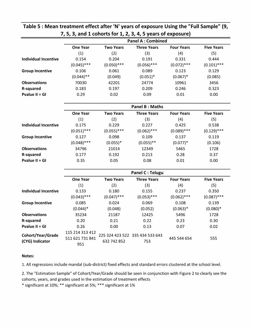
One Year Two Years Three Years Four Years Five Years(1) (2) (3) (4) (5)

Individual Incentive 0.154 0.204 0.191 0.331 0.444(0.045)*** (0.050)*** (0.056)*** (0.072)*** (0.101)***

Group Incentive 0.106 0.061 0.089 0.123 0.129(0.044)** (0.049) (0.051)* (0.067)* (0.085)

Observations 70030 42201 24774 10961 3456R-squared 0.183 0.197 0.209 0.246 0.323Pvalue II = GI 0.29 0.02 0.09 0.01 0.00

One Year Two Years Three Years Four Years Five Years(1) (2) (3) (4) (5)

Individual Incentive 0.175 0.229 0.227 0.425 0.538(0.051)*** (0.055)*** (0.062)*** (0.089)*** (0.129)***

Group Incentive 0.127 0.098 0.109 0.137 0.119(0.048)*** (0.055)* (0.055)** (0.077)* (0.106)

Observations 34796 21014 12349 5465 1728R-squared 0.177 0.192 0.213 0.28 0.37Pvalue II = GI 0.35 0.05 0.08 0.01 0.00

One Year Two Years Three Years Four Years Five Years(1) (2) (3) (4) (5)

Individual Incentive 0.133 0.180 0.155 0.237 0.350(0.043)*** (0.047)*** (0.053)*** (0.062)*** (0.087)***

Group Incentive 0.085 0.024 0.069 0.108 0.139(0.044)* (0.048) (0.052) (0.063)* (0.080)*

Observations 35234 21187 12425 5496 1728R-squared 0.20 0.21 0.22 0.23 0.30Pvalue II = GI 0.26 0.00 0.13 0.07 0.02

Cohort/Year/Grade (CYG) Indicator

115 214 313 412 511 621 731 841

951

225 324 423 522 632 742 852

335 434 533 643 753

445 544 654 555

Notes:

* significant at 10%; ** significant at 5%; *** significant at 1%

2. The "Estimation Sample" of Cohort/Year/Grade should be seen in conjunction with Figure 2 to clearly see the cohorts, years, and grades used in the estimation of treatment effects

Panel A : Combined

Panel B : Maths

Panel C : Telugu

Table 5 : Mean treatment effect after 'N' years of exposure Using the "Full Sample" (9, 7, 5, 3, and 1 cohorts for 1, 2, 3, 4, 5 years of exposure)

1. All regressions include mandal (sub-district) fixed effects and standard errors clustered at the school level.

One Year Two Years Three Years Four Years Five Years One Year Two Years Three Years Four Years Five YearsPercentage Score on Non-repeats 0.201 0.285 0.247 0.257 0.274 0.342 0.413 0.412 0.388 0.427

(0.006)*** (0.006)*** (0.006)*** (0.008)*** (0.011)*** (0.008)*** (0.007)*** (0.008)*** (0.009)*** (0.011)***Incremental Score on Repeats 0.031 0.071 -0.002 -0.011 0.048 -0.017 0.040 -0.033 -0.147 0.024

(0.004)*** (0.004)*** (0.005) (0.005)** (0.010)*** (0.005)*** (0.005)*** (0.005)*** (0.006)*** (0.012)**Incremental Score on non-repeats II schools 0.035 0.029 0.031 0.063 0.092 0.035 0.030 0.033 0.043 0.073

(0.010)*** (0.011)*** (0.010)*** (0.014)*** (0.023)*** (0.010)*** (0.011)*** (0.011)*** (0.013)*** (0.020)***Incremental Score on repeats II schools 0.047 0.046 0.049 0.089 0.103 0.060 0.048 0.038 0.058 0.054

(0.012)*** (0.013)*** (0.013)*** (0.018)*** (0.024)*** (0.012)*** (0.013)*** (0.013)*** (0.018)*** (0.021)**Incremental Score on non-repeats GI schools 0.028 0.002 0.007 0.019 0.020 0.025 -0.006 0.016 0.022 0.024

(0.009)*** (0.011) (0.010) (0.013) (0.017) (0.011)** (0.011) (0.012) (0.014) (0.017)Incremental Score on repeats GI schools 0.029 0.014 0.023 0.026 0.034 0.055 0.009 0.023 0.016 0.020

(0.012)** (0.012) (0.011)** (0.014)* (0.020)* (0.012)*** (0.013) (0.012)* (0.014) (0.020)Observations 56828 38058 22584 10178 3166 57555 34486 22747 10178 3176R-squared 0.144 0.167 0.132 0.214 0.289 0.142 0.142 0.151 0.242 0.185Fraction of Repeat Questions 15.41% 19.67% 16.37% 16.67% 12.00% 13.95% 12.84% 10.36% 6.52% 6.25%Test For Equality of Treatment Effect for Repeat and Non-repeat Questions in II Schools (F-stat p-value) 0.14 0.01 0.01 0.01 0.59 0.00 0.02 0.42 0.31 0.39Test For Equality of Treatment Effect for Repeat and Non-repeat Questions in GI Schools (F-stat p-value) 0.89 0.07 0.02 0.38 0.41 0.00 0.02 0.43 0.61 0.82

One Year Two Years Three Years Four Years Five Years One Year Two Years Three Years Four Years Five YearsPercentage Score on Non-mcq 0.201 0.292 0.233 0.241 0.295 0.308 0.371 0.348 0.325 0.424

(0.007)*** (0.007)*** (0.006)*** (0.008)*** (0.010)*** (0.007)*** (0.007)*** (0.008)*** (0.009)*** (0.012)***Incremental Score on Mcq 0.028 0.021 0.020 0.057 -0.049 0.107 0.121 0.151 0.119 0.008

(0.005)*** (0.005)*** (0.006)*** (0.008)*** (0.007)*** (0.005)*** (0.005)*** (0.007)*** (0.008)*** (0.008)Incremental Score on non-mcq II schools 0.037 0.031 0.031 0.068 0.087 0.032 0.028 0.031 0.053 0.075

(0.010)*** (0.012)*** (0.011)*** (0.016)*** (0.020)*** (0.010)*** (0.012)** (0.012)** (0.015)*** (0.018)***Incremental Score on mcq II schools 0.037 0.034 0.052 0.095 0.118 0.052 0.044 0.045 0.052 0.079

(0.011)*** (0.012)*** (0.012)*** (0.019)*** (0.023)*** (0.012)*** (0.010)*** (0.013)*** (0.016)*** (0.021)***Incremental Score on non-mcq GI schools 0.027 0.003 0.009 0.016 0.021 0.024 -0.013 0.013 0.010 0.036

(0.010)*** (0.011) (0.010) (0.013) (0.018) (0.010)** (0.012) (0.013) (0.014) (0.017)**Incremental Score on mcq GI schools 0.027 0.012 0.029 0.037 0.025 0.037 0.012 0.029 0.041 0.015

(0.010)*** (0.011) (0.010)*** (0.017)** (0.018) (0.012)*** (0.011) (0.013)** (0.016)** (0.018)Observations 63763 36110 21037 8279 3153 64686 36313 21176 8330 3168R-squared 0.137 0.141 0.165 0.270 0.338 0.192 0.232 0.269 0.260 0.256Fraction of MCQ 22.62% 24.33% 26.99% 27.08% 28% 39.20% 39.19% 37.84% 38.41% 37.50%Test For Equality of Treatment Effect for mcq and Non-mcq Questions in II Schools (F-stat p-value) 0.96 0.66 0.01 0.06 0.01 0.00 0.03 0.17 0.95 0.82Test For Equality of Treatment Effect for mcq and Non-mcq Questions in GI Schools (F-stat p-value) 0.96 0.27 0.01 0.12 0.84 0.08 0.00 0.12 0.02 0.14

Cohort/Year/Grade (CYG) Indicator115 214 313 412 511 621 731 841 951

225 324 423 522 632 742

852

335 434 533 643 753

445 544 654 555115 214 313 412 511 621 731 841 951

225 324 423 522 632 742

852

335 434 533 643 753

445 544 654 555

Notes:

* significant at 10%; ** significant at 5%; *** significant at 1%1. All regressions include mandal (sub-district) fixed effects and standard errors clustered at the school level.

Maths Telugu

Table 6A : "N" Year Impact of Performance Pay by Repeat and Non-Repeat QuestionsDependent Variable : Percentage Test Score

Dependent Variable : Percentage Test Score

Table 6B : "N" Year Impact of Performance Pay by multiple choice and Non-multiple choice questions

Maths Telugu

One year Two Year Three Year Four Year Five Year One year Two Year Three Year Four Year Five Year(1) (2) (3) (4) (5) (6) (7) (8) (9) (10)

baseline maths 0.215 0.155 0.213 0.087 0.225 0.165 0.150 0.130(0.019)*** (0.022)*** (0.031)*** (0.051)* (0.018)*** (0.023)*** (0.033)*** (0.040)***

baseline telugu 0.209 0.220 0.178 0.164 0.288 0.191 0.222 0.139(0.019)*** (0.023)*** (0.035)*** (0.055)*** (0.019)*** (0.024)*** (0.036)*** (0.049)***

Individual Incentives 0.108 0.186 0.114 0.232 0.520 0.126 0.223 0.159 0.198 0.299(0.063)* (0.057)*** (0.056)** (0.068)*** (0.125)*** (0.057)** (0.061)*** (0.057)*** (0.066)*** (0.113)***

Group Incentives 0.114 0.035 0.076 0.168 0.156 0.155 0.131 0.085 0.139 0.086(0.061)* (0.055) (0.054) (0.067)** (0.099) (0.059)*** (0.061)** (0.057) (0.065)** (0.095)

Observations 11765 9081 11133 4997 1592 11765 9081 11133 4997 1592R-squared 0.259 0.189 0.127 0.160 0.306 0.308 0.181 0.134 0.148 0.211Pvalue II = GI 0.93 0.03 0.48 0.41 0.01 0.67 0.20 0.19 0.44 0.08

Cohort/Year/Grade (CYG) Indicator

115 214 313 225 324 423335 434 533

643 753445 544 654 555 115 214 313 225 324 423

335 434 533 643 753

445 544 654 555

Notes:

* significant at 10%; ** significant at 5%; *** significant at 1%

Science Social Science

Table 7: "N" Year Impact of Performance Pay on Non-Incentive Subjects

1. All regressions include mandal (sub-district) fixed effects and standard errors clustered at the school level.

One Year Two Year Three Year Four Year Five Year One Year Two Year Three Year Four Year Five Year

Enrollment 0.197 0.100 0.120 0.095 0.266 0.120 0.059 0.063 -0.067 0.156(0.072)*** (0.075) (0.093) (0.111) (0.148)* (0.076) (0.072) (0.084) (0.101) (0.132)

Infrastructure -0.016 -0.095 -0.022 0.009 -0.032 0.041 -0.003 0.007 -0.076 -0.070(0.033) (0.037)** (0.043) (0.062) (0.097) (0.027) (0.039) (0.044) (0.052) (0.085)

Proximity 0.008 0.014 0.004 0.011 0.214 0.009 0.020 -0.016 0.003 0.156(0.013) (0.015) (0.019) (0.029) (0.030)*** (0.013) (0.015) (0.017) (0.026) (0.037)***

Household Affluence 0.023 0.004 0.032 0.013 -0.017 0.032 0.031 0.040 0.008 0.032(0.020) (0.021) (0.021) (0.031) (0.044) (0.018)* (0.020) (0.021)* (0.037) (0.049)

Parental Literacy -0.019 -0.024 0.017 -0.076 -0.108 -0.008 -0.011 -0.012 -0.035 -0.005(0.018) (0.021) (0.023) (0.038)** (0.059)* (0.019) (0.022) (0.024) (0.036) (0.054)

Male 0.006 -0.042 0.044 0.060 0.066 0.018 0.022 0.004 -0.021 -0.020(0.028) (0.032) (0.045) (0.057) (0.102) (0.028) (0.038) (0.045) (0.083) (0.120)

Baseline Test Score 0.002 0.048 0.031 0.006 0.015 -0.002 0.044 -0.063-0.032 -0.037 -0.045 -0.076 -0.03 -0.038 -0.046 -0.078

Cohort/Year/Grade (CYG) Indicator

115 214 313 412 511 621 731 841 951

225 324 423 522 632 742

852

335 434 533 643 753

445 544 654 555115 214 313 412 511 621 731 841 951

225 324 423 522 632 742

852

335 434 533 643 753

445 544 654 555

CovariatesII

GI

Covariate

II * Covariate

GI * Covariate

ObservationsR-squared

Notes:

* significant at 10%; ** significant at 5%; *** significant at 1%

Individual Incentives Group Incentives

Table 8A: "N" Year Heterogenous Treatment Effects By School and Student Characteristics ("Full Sample")

1. All regressions include mandal (sub-district) fixed effects and standard errors clustered at the school level.

Table 8B: Heterogenous Treatment Effects by Teacher CharacteristicsDependent Variable : Teacher Value Added (using all cohorts and years)

Teacher Education Teacher Training Teacher Experience Teacher Salary Teacher Absence-0.022 -0.120 0.221 0.082 0.132(0.134) (0.129) (0.113)* (0.482) (0.037)***-0.065 -0.211 0.225 0.573 0.064(0.136) (0.137) (0.093)** (0.518) (0.035)*-0.006 -0.052 -0.027 -0.036 -0.119(0.025) (0.029)* (0.020) (0.029) (0.044)***0.049 0.091 -0.035 0.005 0.019

(0.041) (0.046)** (0.044) (0.052) (0.078)0.038 0.098 -0.070 -0.056 -0.020

(0.044) (0.050)** (0.037)* (0.056) (0.066)108560 108560 106592 106674 1385940.057 0.057 0.059 0.058 0.052

Control Schools

Individual Incentive Schools

Group Incentive Schols

P-value (H0: II = Control)

P-value (H0: GI = control)

P-value (H0: II = GI)

Correlation with student test score gains

[1] [2] [3] [4] [5] [6] [7]

Based on School Observation0.28 0.27 0.28 0.15 0.55 0.47 -0.109***0.39 0.42 0.40 0.18 0.42 0.58 0.114***

Based on Teacher Interviews0.22 0.61 0.56 0.00 0.00 0.06 0.108***

0.12 0.35 0.32 0.00 0.00 0.12 0.066**0.15 0.39 0.34 0.00 0.00 0.04 0.108***0.03 0.12 0.11 0.00 0.00 0.65 0.153***0.10 0.29 0.25 0.00 0.00 0.04 0.118***0.06 0.18 0.15 0.00 0.00 0.20 -0.004

2. Teacher absence and active teaching are coded as means over the year (and then averaged across the 5 years)

Table 9: Teacher Behavior (Observation and Interviews)

Teacher Behavior

Teacher Absence (%)Actively Teaching at Point of Observation (%)

Did you do any special preparation for the end of year tests? (% Yes)

Incentive versus Control Schools (All figures in %)

What kind of preparation did you do? (UNPROMPTED) (% Mentioning)

Notes: 1. Each "teacher-year" is treated as one observation with t-tests clustered at the school level.

3. All teacher response variables from the teacher interviews are binary and column 5 reports the correlation between a teacher's stated response and the value added by the teacher that year.

* significant at 10%; ** significant at 5%; *** significant at 1%

Extra HomeworkExtra Classwork

Extra Classes/Teaching Beyond School HoursGave Practice Tests

Paid Special Attention to Weaker Children

GI * discontinued

GI * continued

II * discontinued

II * continued

ObservationsR-squaredP-value (H0: II continued = II discontinued)P-value (H0: GI continued = GI discontinued)

Estimation SampleCohortYearGrade

Combined Maths Telugu Combined Maths TeluguII 0.135 0.164 0.105 0.150 0.181 0.119

(0.031)*** (0.036)*** (0.027)***95% CI [0.074 , 0.196] [0.093 , 0.235] [0.052 , 0.158] [0.037 , 0.264] [0.051 , 0.301] [0.009 , 0.228]

GI 0.064 0.086 0.043 0.048 0.065 0.032(0.028)** (0.031)*** (0.026)

95% CI [0.009 , 0.119] [0.0252 , 0.147] [-0.008 , 0.094] [-0.058 , 0.149] [-0.047 , 0.176] [-0.083 , 0.145]

Constant -0.030 -0.029 -0.032(0.018) (0.021) (0.017)*

Observations 165300 82372 82928R-squared 0.046 0.054 0.041II = GI 0.0288 0.0364 0.0299

Notes:

* significant at 10%; ** significant at 5%; *** significant at 1%

0.01

0.89

4,53

3,4

4,54

4,5

555

0.56

0.24

97940.233

0.01

0.93

(0.095)

0.458(0.111)***

107070.196

48790.249

0.132(0.082)

0.117(0.087)

0.098(0.082)***

0.166(0.078)**

0.158(0.067)**

0.167(0.089)*

0.149(0.087)*

0.443(0.095)***

0.133(0.070)*

0.029(0.073)

0.224

Table 10 : Long-Term Impact of Teacher Incentive Programs on Continued and Discontinued Cohorts

Y3 on Y0 Y4 on Y0 Y5 on Y0

Table 11 : Average "Gross" One-Year Treatment Effect of Teacher Incentive Programs

Panel A: OLS with Estimated gammaPanel B: Average non-parametric Treatment Effect

(Based on Figure 4)

1. All regressions in Panel A include mandal (sub-district) fixed effects and standard errors clustered at the school level