Long-Range Transformers for Dynamic Spatiotemporal Forecasting

Jake Grigsby, Zhe Wang, Yanjun QiUniveristy of Virginia

{jcg6dn, zw6sg, yanjun}@virginia.edu

Abstract

Multivariate Time Series Forecasting (TSF) focuses onthe prediction of future values based on historical con-text. In these problems, dependent variables provide ad-ditional information or early warning signs of changesin future behavior. State-of-the-art forecasting modelsrely on neural attention between timesteps. This al-lows for temporal learning but fails to consider distinctspatial relationships between variables. This paper ad-dresses the problem by translating multivariate TSF intoa novel “spatiotemporal sequence” formulation whereeach input token represents the value of a single vari-able at a given timestep. Long-Range Transformers canthen learn interactions between space, time, and valueinformation jointly along this extended sequence. Ourmethod, which we call Spacetimeformer, scales tohigh dimensional forecasting problems dominated byGraph Neural Networks that rely on predefined vari-able graphs. We achieve competitive results on bench-marks from traffic forecasting to electricity demand andweather prediction while learning spatial and temporalrelationships purely from data.

1 Introduction

Multivariate forecasting attempts to predict future outcomesbased on historical context and has direct applications tomany domains, including science, policy, and business.Jointly modeling a set of variables allows us to interpretdependency relationships that provide additional context orearly warning signs for changes in future behavior. Time Se-ries Forecasting (TSF) models typically deal with a smallnumber of variables with long-term temporal dependen-cies that require historical recall and distant forecasting.This is commonly handled by encoder-decoder sequence-to-sequence (Seq2Seq) architectures (Sec 2.1). The relation-ships between input variables are usually unknown, sparse,or time-dependent. Examples include many health and fi-nance applications. In these cases, we are forced to dis-cover variable relationships from data. Current state-of-the-art TSF models substitute classic Seq2Seq architecturesfor neural-attention-based mechanisms (Zhou et al. 2021).However, these models represent the value of multiple vari-

ables per timestep as a single input token1. This only allowsthem to learn “temporal attention” amongst timesteps, andcan ignore the distinct spatial 2 relationships that exist be-tween variables.

In this paper, we propose to flatten multivariate inputs intolong sequences where each input token isolates the valueof a single variable at a given timestep. The resulting in-put allows Long-Range Transformer architectures to learnself-attention networks across both space and time jointly.This creates a “spatiotemporal attention” mechanism. Fig-ure 1 illustrates the distinction between temporal and spa-tiotemporal attention. Our method can interpret long con-text windows and forecast many timesteps into the futurewhile also discovering the spatial relationships between hun-dreds of variables. The spatial scalability of our model sug-gests applications to the kinds of forecasting problems cur-rently dominated by Graph Neural Network (GNN) meth-ods. GNNs rely on predefined graphs representing the rela-tionships between input variables. We empirically show thatspatiotemporal sequence learning with Transformers can re-cover the relationships necessary to achieve competitive per-formance on these tasks while learning spatial and tempo-ral connections purely from data. We evaluate the techniquein various domains spanning the spatiotemporal spectrumfrom traffic forecasting to electricity production and long-term weather prediction.

2 Background and Related Work2.1 Deep Learning in Time Series ForecastingTSF in practice is often focused on business/finance appli-cations and utilizes relatively simple but reliable statisti-cal methods (Box et al. 2015) (Taylor and Letham 2018).Analogous to the trend in areas like Vision and NaturalLanguage Processing (NLP), hand-crafted approaches havebegun to be replaced by Deep Learning techniques (Smyl2020). This is particularly true in multivariate forecasting,

1An input token is one element of a Transformer’s input se-quence. Multihead Self-Attention (Sec 2.2) learns representationsby sharing information between tokens.

2In most real-world forecasting tasks, variables spatially closeto one another exhibit similar patterns. We use the word “spatial”to refer to such relationships between multiple variables generally.

arX

iv:2

109.

1221

8v1

[cs

.LG

] 2

4 Se

p 20

21

where the relationships between multiple time series chal-lenge traditional models’ ability to scale (Lim and Zohren2021) (Benidis et al. 2020). Deep Learning approaches toTSF are generally based on a Seq2Seq framework in whicha context window of the recent past is mapped to a targetwindow of predictions for the future. More formally: givena sequence of time inputs {xT−c, . . . , xT } and variable(s){yT−c, . . . ,yT } up to time T , we output another sequenceof variable values {yT+1, . . . , yT+t} corresponding to ourpredictions at future timesteps {xT+1, . . . , xT+t}.

The most common class of deep TSF models are based ona combination of Recurrent Neural Networks (RNNs) andone-dimensional convolutions (Conv1Ds) (Borovykh, Bo-hte, and Oosterlee 2017) (Smyl 2020) (Salinas, Flunkert,and Gasthaus 2019) (Lai et al. 2018). More related to theproposed method is a recent line of work on attention mech-anisms that aim to overcome RNNs’ autoregressive trainingand difficulty in interpreting long-term patterns (Iwata andKumagai 2020) (Li et al. 2019) (Zerveas et al. 2020) (Wuet al. 2020a) (Oreshkin et al. 2020). Notable among theseis the Informer (Zhou et al. 2021) - a general encoder-decoder Transformer architecture for TSF. Informer en-codes time series inputs with learned temporal embeddingsand appends a start token3 to the decoder sequence of zerosthat need prediction.

2.2 Long-Range TransformersThe Transformer (Vaswani et al. 2017) is a Deep Learn-ing architecture for sequence-to-sequence prediction that iswidely used in NLP (Devlin et al. 2019). Transformers arecentered around the multi-head self-attention (MSA) mecha-nism. A sequence (x) consisting of L input tokens generatesd-dimensional query, key, and value vectors with learnedfeed-forward layers denoted WQ, WK , and WV , respec-tively. The scaled dot-product of tokens’ query and key vec-tors determines the attention given to values along the inputsequence according to Eq 1.

MSA(x) = softmax(WQ(x)WK(x)√

d

)WV (x) (1)

MSA learns weighted relationships between its inputs in or-der to pass information between tokens. This idea has ap-pealing similarity to passing messages across a weightedadjacency matrix (a graph) (Joshi 2020) (Liu et al. 2019).Because MSA matches each query to the keys of the en-tire sequence, its runtime and memory use grows quadrati-cally with the length of its input. This becomes a significantobstacle in long-input domains where self-attention mightotherwise be a promising solution, including document clas-sification (Pappagari et al. 2019), summarization (Manakuland Gales 2021), and protein sequence analysis (Lanchantinet al. 2021). As a result, the research community has racedto develop and evaluate MSA-variants for longer sequences(Tay et al. 2020). Many of these methods introduce heuris-tics to sparsify the attention matrix. For example, we can at-

3The start token is probably better described as a “start tokensequence” because unlike special-purpose start tokens in NLP it isa sequence of the final tokens of the context window.

tend primarily to adjacent input tokens (Li et al. 2019), selectglobal tokens (Guo et al. 2019), increasingly distant tokens(Ye et al. 2019) (Child et al. 2019) or a combination thereof(Zaheer et al. 2020) (Zhang et al. 2021). While these meth-ods are effective, their inductive biases about the structure ofthe trained attention matrix are not always compatible withtasks outside of NLP.

Another approach looks to approximate MSA in sub-quadratic time while retaining its flexibility (Wang et al.2020) (Zhou et al. 2021) (Xiong et al. 2021) (Zhu et al.2021). Particularly relevant to this work is the Performer(Choromanski et al. 2021). Performer approximatesMSA in linear space and time with a kernel of random or-thogonal features and enables the long-sequence approachthat is central to our work.

2.3 Spatiotemporal ForecastingMultivariate TSF involves two axes of complexity: the fore-cast sequence’s duration, L, and the number of variables Nconsidered at each timestep. As N grows, it becomes in-creasingly important to model the spatial relationships be-tween each variable explicitly. Recent TSF methods struc-ture their input as (xt,yt) concatenated vectors of multiplevariable values per timestep. Attention-based models needto connect the variable values at a given timestep to entiretimesteps in the past. However, the variables we are mod-eling may have different periodicities and relations to oneanother.

To better explain this, we introduce a TSF problem laterused in our experiments. Suppose we are forecasting the airtemperature at weather stations in the United States. Severalstations are located relatively close to each other in centralTexas. The rest are also clustered together but centered hun-dreds of miles away outside New York City. The two groupsexperience different weather patterns as a result of their ge-ographic separation. In order to predict future weather pat-terns in Texas, we may need to attend to the values of nearbystations when the current weather cycle began. However, thismay have occurred before the information that is relevant tothe stations in New York. When faced with this problem, atemporal attention model would be forced to “average” theserequirements and attend to timesteps somewhere in the mid-dle - a compromise that provides little relevant informationto either situation. The NY-TX weather problem is unreal-istic in the sense that it is unlikely that a real-world systemwould attempt to jointly model such unrelated sequences.However, this problem can appear more subtly in domainswhere the relationships between the series are unknown ordifficult to predict.

There have been a number of approaches that confrontthis problem in the context of RNN-based attention (Shih,Sun, and Lee 2019) (Gangopadhyay et al. 2021) (Qin et al.2017). These models alternate between separate spatial andtemporal layers. There are several works extending MSA tosimilar ‘spatial, then temporal’ architectures (Xu et al. 2021)(Cai et al. 2020) (Park et al. 2020) (Plizzari, Cannici, andMatteucci 2021), but they rely on the predefined variablegraphs common in the GNN literature (see Sec 3.3). Furtherdiscussion is moved to Appendix A.

T-3

T-3T-2T-3 TT-1

T-3

T-2

T-2

T-2

T-1

T-1

T-1

T

T

T

Query Token

Time Series Variables Less

AttentionMore

Attention

Query Token

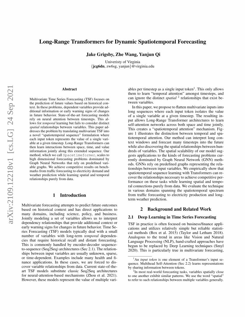
Figure 1: Temporal learning (left) versus Spatiotemporallearning (right): Splitting the variables into separate tokenscreates a spatiotemporal graph where we can attend to dif-ferent timesteps for each variable.

3 Method3.1 Spatiotemporal Forecasting with

TransformersThe temporal attention compromise discussed in Sec 2.3can be blamed on the fact that we are representing mul-tiple variables per token. It is important to note that thisdilemma is unique to applications of Transformers outsideof NLP. In the NLP setting, every token of the input se-quence represents one individual idea (e.g., a single word).However, multivariate TSF inherently models multiple dis-tinct sequences per timestep (Shih, Sun, and Lee 2019). Thesolution, then, is to recover the “one-idea-per-token” formatof NLP. We can do this by separating (xt,yt) inputs into asub-sequence of {(xt, yit), . . . , (xt, yNt )} tokens, where Nis the number of variables we are modeling. The resultingsequence is N times longer but represents each node of thespatiotemporal graph as an individual token. Assuming ourattention mechanism can scale with the additional length, itcan now learn unique relationships for every variable. Thedistinction is depicted in Figure 1.

After flattening the input variables, we need to allowTransformers to correctly interpret the variable each tokenoriginates from as well as its time and scalar value. Trans-formers are permutation invariant, meaning they cannot in-terpret the order of input tokens by default. This is fixed byadding a position embedding to the tokens - usually with afixed sinusoidal pattern (Vaswani et al. 2017). In our flat-tened representation, N tokens should have the same posi-tion. This could be solved with a modified positional em-bedding that accounts for the flattened sequence. However,a fixed positional embedding only preserves relative order.In the NLP context, relative position is all that matters, butin a time series problem, the input sequence takes place ina specific window of time that may be relevant to long-termseasonal patterns. For example, it is important to know therelative order of three weeks of temperature observations,but it is also important to know that those three weeks takeplace in late spring when temperatures are typically rising.We achieve this by learning positional embeddings basedon a Time2Vec layer (Kazemi et al. 2019). Time2Vecpasses a representation of absolute time (e.g., the calendardatetime) through sinusoidal patterns of learned offsets andwavelengths. This helps represent periodic relationships that

are relevant to accurate predictions. We also append a rel-ative order index to the time input values4. The concate-nated timeseries value and time embedding are then pro-jected to the input dimension of the Transformer model witha feed-forward layer. We refer to the resulting output as the“Value&Time Embedding.”

Now that the model can distinguish between timesteps, italso has to tell the difference between the variables at each ofthose timesteps. We add a “Variable Embedding” to each to-ken. The variable embedding indicates the time series fromwhich each token originates. This is implemented as a stan-dard embedding layer that maps the integer index of eachseries to a higher-dimensional representation as is commonfor word embeddings in NLP.

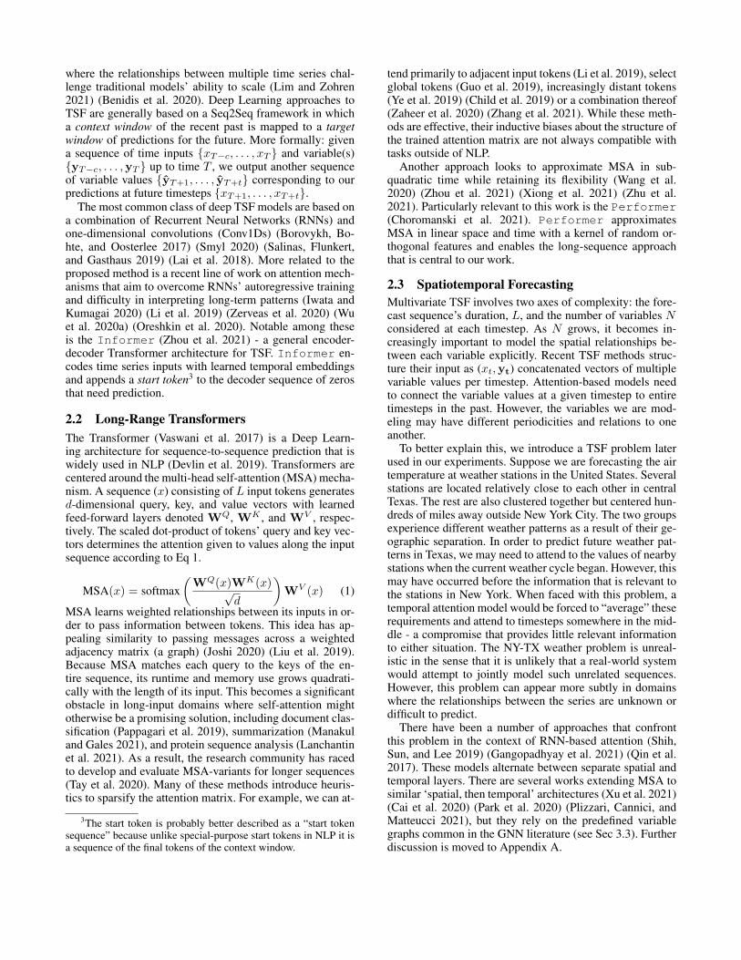
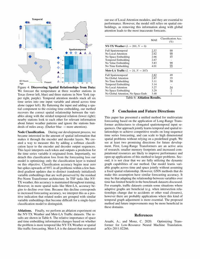
A final consideration is the representation of missingtimeseries values that the model is tasked to predict. Theencoder observes the context sequence in which all valuesare present. However, the decoder deals with missing val-ues that need prediction in addition to the start token ofthe last few timesteps of the context sequence (as in theInformer (Zhou et al. 2021) model). We pass missingvalues as a zero vector and resolve ambiguity between truecontext/start-token values of zero and missing tokens with abinary “Given embedding”5. The Value&Time, Space, andGiven embeddings sum to create the encoded sequence. Theentire pipeline is represented visually in Figure 2.

3.2 Long-Range Transformers for Real-WorldSpatiotemporal Forecasting

After the spatiotemporal embedding, the sequence is readyto be fed through a standard Transformer encoder-decoder.Our method does not assume access to predefined variablerelationships or even that those relationships remain fixedover time; the embedding represents the spatiotemporalforecasting problem in a raw format that puts full faith in thelearning power of the Transformer architecture. This mayraise questions as to why this approach has not been tried be-fore; the answer rests heavily on scale and timing. The em-bedding in Sec 3.1 converts a sequence-to-sequence problemof length L into a new one of length LN . Vanilla MSA lay-ers have a maximum sequence length of less than 1, 000 -and on hardware aside from the highest-end GPUs/TPUs weare limited to something closer to ∼ 500. The spatiotempo-ral sequence lengths considered in our experimental resultsexceed 23, 000. Clearly, additional optimization is needed tomake these problems feasible.

Scaling with Fast-Attention. However, we are fortunatethat there is a rapidly-developing field of research in long-sequence transformers (Sec 2.2). We modify open-sourceimplementations of fast-attention mechanisms in an effort

4This is helpful when the data are taken at close intervals suchthat most entries of the resulting Time2Vec output vectors areidentical. In the extreme case, it serves as a fail-safe for datasetsthat do not provide distinct timestamps for each datapoint, e.g.,when all observations occur on the same day but the hour andminute values are not recorded.

5The Given embedding is not used in Informer and is notoften relevant in practice. It resolves an edge case for datasets thatnaturally contain zero values.

1 21

5

2 3

6

Initial Sequence Time Embedding Variable Embedding0

Spatiotemporal SequenceValue & Time Embedding

“Given”Embedding 4

Figure 2: Input Encoding Pipeline: (1) The standard multivariate input format with time information included. Decoder inputshave missing (“?”) values set to zero where predictions will be made. (2) The time sequence is passed through a Time2Veclayer to generate a frequency embedding that represents periodic input patterns. (3) A binary embedding indicates whetherthis value is given as context or needs to be predicted. (4) The integer index of each time series is mapped to a “spatial”representation with a lookup-table embedding. (5) The Time2Vec embedding and variable values of each time series areprojected with a feed-forward layer. (6) Value&Time, Variable, and Given embeddings are summed and laid out s.t. MSAattends to relationships across both time and variable space at the cost of a longer input sequence.

7DUJHW�(PEHGGLQJ&RQWH[W�(PEHGGLQJ

1RUP

/RFDO�6HOI�$WWQ /RFDO�6HOI�$WWQ

1RUP

1RUP

1RUP

1RUP

1RUP

1RUP

1RUP

1RUP

1RUP

*OREDO�6HOI�$WWQ *OREDO�6HOI�$WWQ

/LQHDU

/LQHDU

/LQHDU

/RFDO�&URVV�$WWQ

*OREDO�&URVV�$WWQ

(QFRGHG�6HTXHQFH

2XWSXW�6HTXHQFH

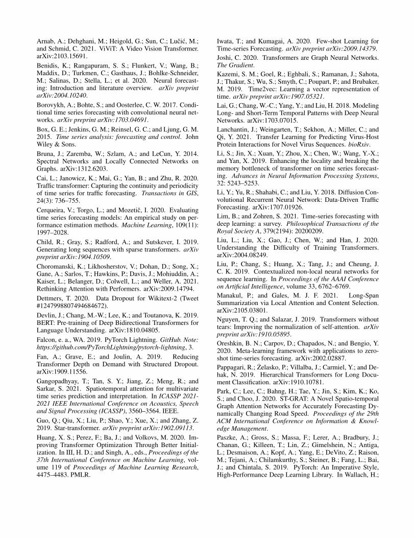
Figure 3: The Spacetimeformer architecture for jointspatiotemporal sequence learning.

to scale our model. Informer (Zhou et al. 2021) proposesProbSparse attention. While this method is faster andmore scalable than vanilla MSA, we are only able to reachsequences between 1k-2k tokens, mostly because it is onlyapplicable to self-attention modules. Instead, we opt for thePerformer FAVOR+ attention (Choromanski et al. 2021)- a linear approximation of softmax6 attention using a ran-

6In practice we find that the generalized ReLU kernel variant isslightly more memory efficient and use that as our default attentionmechanism.

dom kernel method. The experiments in this paper are per-formed on four 8− 12GB GPUs - significantly less memorythan the maximum currently available (e.g., larger clustersof V100s, TPUs). This constraint is likely to be less rele-vant as hardware development continues to shift towards in-tensive Deep Learning. However, we find that a multi-GPUPerformer setup is enough to tackle all but the longestspatiotemporal sequences.

Scaling with Initial and Intermediate Conv1Ds. In thelongest-sequence problems, we can also look for ways tolearn shorter representations of the input to save memory.This is only applicable to the context window encoder,but in practice the context window is typically the bottle-neck. We can learn to summarize the sequence with stridedone-dimensional convolutions; we use the proper stride andpadding to cut sequence length in half per Conv1D layer.“Initial” convolutions are applied to the Value&Time em-bedding while the variable embedding tokens are repeatedfor half their usual length. “Intermediate” convolutions oc-cur between MSA layers. Intermediate convolutions are akey component of the Informer (Zhou et al. 2021) archi-tecture. However, our embedding creates an undesirable em-phasis on the order of the flattened variable tokens. We ad-dress this by passing each variable’s full sequence throughthe convolution independently (halving their length) andthen recombining them into the longer spatiotemporal se-quence. We prefer to learn the full-size spatiotemporal graphwhen it fits in memory. Therefore none of the reported re-sults use intermediate convolutions; the longest dataset (ALSolar) model uses one initial convolution.

Local and Global Attention. We empirically find thatlearning an attention layer over a longer global sequence

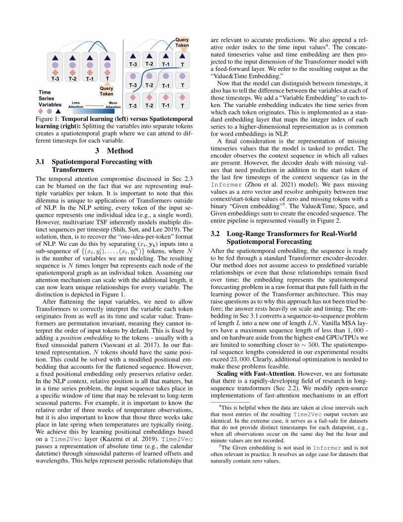
eliminates a helpful local bias that hurts performance inproblems with largeN . We address this by adding additional“local” attention modules to each encoder and decoder layer.Each variable sequence attends to itself first before attendingto global tokens. Note that this does mean we are simplifyingthe global attention layer by separating temporal and spatialattention, as is common in the methods discussed above inaddition to Video Transformers (Arnab et al. 2021) and otherlong-range NLP architectures (Zhu et al. 2021) (Zhang et al.2021). Rather, every token attends to every token in its ownsequence and then to every token in the entire spatiotempo-ral global sequence. We use a Pre-Norm architecture (Xionget al. 2020) and BatchNorm normalization rather than thestandard LayerNorm and other alternatives in the litera-ture. Additional implementation details are discussed in Ap-pendix C. A one-layer encoder-decoder architecture is de-picted in Figure 3.

Output and Loss Functions. The final feed-forwardlayer of the decoder generates a two-dimensional vector thatparameterizes the mean and standard deviation of a Normaldistribution. This sequence of distributions is folded backinto the original input format of (xt, yt), and the timestepscorresponding to predictions on the start tokens are dis-carded. We can then optimize a variety of forecasting lossfunctions, depending on the particular problem and the base-lines we are comparing against. Explanations of commonloss functions can also be found in Appendix C.

Because of all this additional engineering, we avoid di-rect comparisons to Informer although it is a key inspi-ration and closely related work. Instead, our most directbaseline is a version of our model that follows a “temporal-only” embedding scheme similar to Informer’s. The se-quence is never flattened into distinct spatial tokens; theValue&Time embedding input includes all the time seriesvalues concatenated together as normal, and there is no spa-tial embedding. There is no concept of “local vs. global” inthis setup, so we skip the local attention modules. We typi-cally compensate for parameter count differences with addi-tional encoder/decoder layers. We nickname our model theSpacetimeformer for clarity in experimental results.

3.3 Connecting to Spatial Forecasting and GNNsAs N approaches and then exceeds L, e.g., in traffic fore-casting, we begin to enter the territory of Graph Neural Net-works (Wu et al. 2021a). In this context, GNNs are multi-variate forecasting models where the relationship betweenthe time series can be provided in advance (e.g., a mapof connected roads) (Liu et al. 2019) (Li et al. 2018). Atypical forecasting GNN involves iterative applications ofgraph message passing between nodes (e.g., Graph Convo-lutional Network layers (Bruna et al. 2014)) followed by anRNN/Conv1D for temporal learning amongst the timestepsof each node individually. For a representative example andthorough explanation see DCRNN (Li et al. 2018).

This paper approaches multivariate prediction with Trans-formers from a TSF perspective where spatial relationshipsshould be explicitly modeled, but their relationships are un-known and must be learned during training. We proposea novel input embedding and architecture for Transform-

Variables(N )

Length(L)

Size(Timesteps)

NY-TX Weather 6 800 569,443Toy Dataset 20 160 2,000AL Solar 137 192 52,560Metr-LA Traffic 207 24 34,272Pems-Bay Traffic 325 24 52,116

Table 1: Dataset Summary.

ers that jointly learn spatial and temporal attention alongan extended spatiotemporal sequence. In this way, we blurthe distinction between TSF and GNN models. MTGNN (Wuet al. 2020b) is a related work in this hybrid category thatlearns an adjacency matrix from data before applying GNN-style spatial/temporal convolutions. However, it still sepa-rates spatial and temporal learning and is not as capable as atemporal forecaster because its one-shot convolutional pre-diction module does not scale with L like a TSF method.Our method retains the temporal forecasting ability of a TSFmodel while recovering the spatial relationships of a GNNmodel and avoiding the assumption of a predefined graph.

4 ExperimentsWe evaluate our method in five datasets, including traf-fic forecasting, weather prediction, solar energy production,and a simple toy example. Descriptions of each task canbe found in Appendix B, and a summary of key informa-tion is provided in Table 1. We compare against represen-tative methods from the TSF and GNN literature in addi-tion to ablations of our model. These include the previ-ously mentioned MTGNN model and Temporal ablation,as well as a basic autoregressive linear model (LinearAR), a standard encoder-decoder LSTM without attention,and a CNN/Conv1D-based LSTNet (Lai et al. 2018). SeeAppendix C.2 for details. Hyperparameter information forSpacetimeformer models can be found in AppendixC.1. All results average at least three random seeds, withadditional runs collected when variance is non-negligible.All models use the same training loop, dataset code, andevaluation process to ensure a fair comparison. We also addTime2Vec information to baseline inputs when applicablebecause it has been shown to improve the performance of avariety of sequence models (Kazemi et al. 2019).

Toy Dataset. We begin with a toy dataset inspired by(Shih, Sun, and Lee 2019) consisting of a multivariate sine-wave sequence with strong inter-variable dependence. Moredetails can be found in Appendix B. Several ablations ofour method are considered. Temporal modifies the spa-tiotemporal embedding as discussed at the end of Sec 3.2.ST Local skips the global attention layers but includesspatial information in the embedding. The “Deeper” vari-ants attempt to compensate for the additional parameters ofthe local+global attention architecture of our full method.All models use a small Transformer model and optimizefor MSE. The final quarter of the time series is held outas a test set; a similar test split is used in all experiments(Cerqueira, Torgo, and Mozetic 2020). The results are shown

Temporal Temporal(Deeper)

Temporal(Deeper &Full Attn)

ST Local ST Local(Deeper) Spacetimeformer

MSE 0.006 0.010 0.005 0.021 0.014 0.003MAE 0.056 0.070 0.056 0.104 0.090 0.042RRSE 0.093 0.129 0.094 0.180 0.153 0.070

Table 2: Toy Dataset Results. We indicate the loss functionmetric (here, MSE) with italics in subsequent tables.

in Table 2. The Temporal embedding is forced to compro-mise its attention over timesteps in a way that reduces pre-dictive power over variables with such distinct frequencies.Standard (“Full”) attention fits in memory with the Tempo-ral embedding but is well approximated by Performer.Our method learns an uncompromising spatiotemporal re-lationship among all tokens to generate the most accuratepredictions by all three metrics.

NY-TX Weather. We evaluate each model on a customdataset of temperature values collected from the ASOSWeather Network. As described in our Sec 2.3 example, weuse three stations in central Texas and three in eastern NewYork. Temperature values are taken at one-hour intervals,and we investigate the impact of sequence length by predict-ing 40, 80, and 160 hour target sequences. The results areshown in Table 3. Our spatiotemporal embedding schemeprovides the most accurate forecasts, and its improvementover the Temporal method appears to increase over longersequences where the temporal attention compromise may bemore relevant. LSTM is the most competitive baseline. Thisis not surprising given that this problem lies towards theTSF end of the spatiotemporal spectrum, where LSTMs area common default. The success of MTGNN is more surprisingbecause we are using it at sequence lengths far longer thanconsidered in the original paper (Wu et al. 2020b). However,its convolution-only output mechanism begins to struggle atthe 80 and 160 hour lengths.

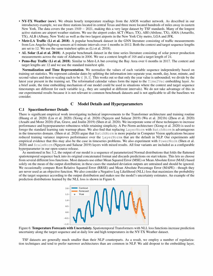
We use the NY-TX weather dataset to experiment witha Negative Log Likelihood (NLL) loss that maximizes theprobability of the target sequence and makes use of our out-put distributions’ uncertainty estimates. The model learns anintuitive prediction strategy that generally increases uncer-tainty along the target sequence. It also adds uncertainty toinflection points where temperatures are reaching daily lowsor highs. An example prediction plot for one of the stationsis shown in Appendix C.1 Figure 6.

Linear AR LSTM MTGNN Temporal Spacetimeformer

40 hoursMSE 18.84 14.29 13.32 13.29 12.49MAE 3.24 2.84 2.67 2.67 2.57RRSE 0.40 0.355 0.34 0.34 0.33

80 hoursMSE 23.99 18.75 19.27 19.99 17.9MAE 3.72 3.29 3.31 3.37 3.19RRSE 0.45 0.40 0.41 0.41 0.40

160 hoursMSE 28.84 22.11 24.28 24.16 21.35MAE 4.13 3.63 3.78 3.77 3.51RRSE 0.50 0.44 0.46 0.46 0.44

Table 3: NY-TX Weather Results.

AL Solar. We turn our focus to problems on the GNN endof the spatiotemporal spectrum where N > L. The AL So-lar dataset is a middle ground that is still studied in the TSFliterature (Lai et al. 2018) and consists of solar power pro-duction measurements taken at 10-minute intervals from 137locations. We predict 4-hour sequences and the results areshown in Table 4. Our method is significantly more accu-rate than the TSF baselines. We speculate that this is dueto an increased ability to forecast unusual changes in powerproduction due to weather or other localized effects. MTGNNlearns similar spatial relationships, but its temporal predic-tions are not as accurate.

Linear AR LSTNet LSTM MTGNN Temporal Spacetimeformer

MSE 14.3 15.09 14.35 11.40 14.3 8.96MAE 2.29 2.08 2.02 1.76 1.85 1.43

Table 4: AL Solar Results.

Traffic Prediction. Next, we experiment on two datasetscommon in GNN research. The Metr-LA and Pems-Baydatasets consist of traffic speed readings at 5 minute inter-vals. We forecast the conditions for the next hour. In additionto the baselines in our research code, we include scores fromthe original DCRNN GNN model for context. Our methodclearly separates itself from TSF models and enters the per-formance band of dedicated GNN methods - even those thatrely on predefined road graphs.

Time Series Models GNN Models

Linear AR LSTM LSTNet Temporal DCRNN MTGNN Spacetimeformer

Metr-LAMAE 4.28 3.34 3.36 3.14 3.03 2.92 2.82MSE 91.57 48.19 44.23 41.88 37.88 39 36.21MAPE 11.11 9.89 9.53 8.9 8.27 8.46 7.71

Pems-BayMAE 2.24 2.41 2.03 2.37 1.59 1.75 1.73MSE 27.62 25.49 19.17 23.52 12.81 15.23 14.37MAPE 4.98 5.81 4.68 5.52 3.61 4.08 3.85

Table 5: Traffic Forecasting Results.

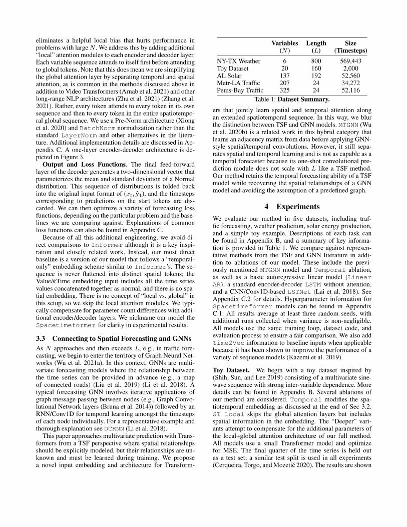
Spatiotemporal Attention Patterns. Our method relieson approximate attention mechanisms that never explicitlycompute the attention matrix. However, we use a trick de-scribed in the Performer appendix (Choromanski et al.2021) to visualize attention patterns. Standard TemporalTransformers learn sliding patterns that resemble convolu-tions. These wave-like patterns are the result of Time2Vecinformation in the input. Our method learns distinct connec-tions between variables - this leads to attention diagrams thattend to be structured in “variable blocks” due to the way weflatten our input sequence. Figure 4 provides an annotatedexample for the NY-TX weather dataset. If viewing a digitalcopy of this paper, the reader may be able to zoom in andsee the wave-like temporal patterns that exist within each“block” of variable attention. Our method learns spatial at-tention over blocks of variable inputs and convolution-styletemporal attention over the timesteps within each variable.Some attention heads convincingly recover the ground-truthrelationship between input variables in the NY-TX weatherdataset. GNN-level performance in highly spatial tasks liketraffic forecasting supports a similar conclusion for morecomplex graphs.

���+RXUV�$JR 3UHVHQW

«������

«������

7HPSRUDO

6SDWLRWHPSRUDO

Figure 4: Discovering Spatial Relationships from Data:We forecast the temperature at three weather stations inTexas (lower left, blue) and three stations in New York (up-per right, purple). Temporal attention models stack all sixtime series into one input variable and attend across timealone (upper left). By flattening the input and adding a spa-tial component to the existing time embedding, our methodrecovers the correct spatial relationship between the vari-ables along with the strided temporal relation (lower right);nearby stations look to each other for relevant informationabout future weather patterns and ignore the stations hun-dreds of miles away. (Darker blue→ more attention).

Node Classification. During our development process, webecame interested in the amount of spatial information thatmakes it through the encoder and decoder layers. We cre-ated a way to measure this by adding a softmax classifi-cation layer to the encoder and decoder output sequences.This layer interprets each token and outputs a prediction forthe time series variable it originated from. Importantly, wedetach this classification loss from the forecasting loss ourmodel is optimizing; only the classification layer is trainedon this objective. Classification accuracy begins near zerobut spikes upwards of 99% in all problems within a few hun-dred gradient updates due to distinct (randomly initialized)variable embeddings that are well-preserved by the residualPre-Norm Transformer architecture. In TSF tasks like NY-TX weather, this accuracy is maintained throughout training.However, in more spatial tasks like Metr-LA, accuracy be-gins to decline over time. Because this decline correspondsto increased forecasting accuracy, we interpret this as a pos-itive indication that related nodes are grouped with similarvariable embeddings that become difficult for a single-layerclassification model to distinguish.

Ablations. Finally, we perform an ablation experiment onthe NY-TX Weather and Metr-LA Traffic datasets. The re-sults are shown in Table 6. The relative importance of spaceand time embedding information changes based on whetherthe problem is more temporal like NY-TX Weather or spatiallike traffic forecasting. Metr-LA is the dataset that motivated

our use of Local Attention modules, and they are essential toperformance. However, the model still relies on spatial em-beddings, as removing this information along with globalattention leads to the most inaccurate forecasts.

MAE Classification Acc.(%)

NY-TX Weather (L = 200, N = 6)Full Spatiotemporal 2.57 99No Local Attention 2.62 99No Space Embedding 2.66 45Temporal Embedding 2.67 -No Value Embedding 3.83 99No Time Embedding 4.01 99

Metr-LA Traffic (L = 24, N = 207)Full Spatiotemporal 2.82 49No Global Attention 2.87 35No Time Embedding 3.11 50Temporal Embedding 3.14 -No Local Attention 3.27 54No Space Embedding 3.29 2No Global Attention, No Space Emb. 3.48 1

Table 6: Ablation Results.

5 Conclusion and Future DirectionsThis paper has presented a unified method for multivariateforecasting based on the application of Long-Range Trans-former architectures to elongated spatiotemporal input se-quences. Our approach jointly learns temporal and spatial re-lationships to achieve competitive results on long-sequencetime series forecasting, and can scale to high dimensionalspatial problems without relying on a predefined graph. Wesee at least two promising directions for future develop-ment. First, Long-Range Transformers are an active areaof research; smaller memory footprints and increased com-putational resources are likely to improve performance andopen up applications of this method to larger problems. Sec-ond, it is not clear that we are fully utilizing the dynamicgraph capabilities of our method. Our model learns vari-able graphs across time and space jointly without assuminga fixed spatial relationship. However, GNN methods that domake this assumption have similar forecasting accuracy. Itmay be that adapting the relationship between variables overtime has limited benefit in the benchmark datasets discussed.For example, traffic datasets contain some situations whereadaptive graphs are beneficial (e.g. when intersection rela-tionships change due to accidents or other road closures),however there are probably applications where this kind oftemporal graph adjustment is more essential. The proposedmethod and future improvements may be more beneficial inthese domains.

ReferencesAraabi, A.; and Monz, C. 2020. Optimizing Trans-former for Low-Resource Neural Machine Translation.arXiv:2011.02266.

Arnab, A.; Dehghani, M.; Heigold, G.; Sun, C.; Lucic, M.;and Schmid, C. 2021. ViViT: A Video Vision Transformer.arXiv:2103.15691.Benidis, K.; Rangapuram, S. S.; Flunkert, V.; Wang, B.;Maddix, D.; Turkmen, C.; Gasthaus, J.; Bohlke-Schneider,M.; Salinas, D.; Stella, L.; et al. 2020. Neural forecast-ing: Introduction and literature overview. arXiv preprintarXiv:2004.10240.Borovykh, A.; Bohte, S.; and Oosterlee, C. W. 2017. Condi-tional time series forecasting with convolutional neural net-works. arXiv preprint arXiv:1703.04691.Box, G. E.; Jenkins, G. M.; Reinsel, G. C.; and Ljung, G. M.2015. Time series analysis: forecasting and control. JohnWiley & Sons.Bruna, J.; Zaremba, W.; Szlam, A.; and LeCun, Y. 2014.Spectral Networks and Locally Connected Networks onGraphs. arXiv:1312.6203.Cai, L.; Janowicz, K.; Mai, G.; Yan, B.; and Zhu, R. 2020.Traffic transformer: Capturing the continuity and periodicityof time series for traffic forecasting. Transactions in GIS,24(3): 736–755.Cerqueira, V.; Torgo, L.; and Mozetic, I. 2020. Evaluatingtime series forecasting models: An empirical study on per-formance estimation methods. Machine Learning, 109(11):1997–2028.Child, R.; Gray, S.; Radford, A.; and Sutskever, I. 2019.Generating long sequences with sparse transformers. arXivpreprint arXiv:1904.10509.Choromanski, K.; Likhosherstov, V.; Dohan, D.; Song, X.;Gane, A.; Sarlos, T.; Hawkins, P.; Davis, J.; Mohiuddin, A.;Kaiser, L.; Belanger, D.; Colwell, L.; and Weller, A. 2021.Rethinking Attention with Performers. arXiv:2009.14794.Dettmers, T. 2020. Data Dropout for Wikitext-2 (Tweet#1247998807494684672).Devlin, J.; Chang, M.-W.; Lee, K.; and Toutanova, K. 2019.BERT: Pre-training of Deep Bidirectional Transformers forLanguage Understanding. arXiv:1810.04805.Falcon, e. a., WA. 2019. PyTorch Lightning. GitHub. Note:https://github.com/PyTorchLightning/pytorch-lightning, 3.Fan, A.; Grave, E.; and Joulin, A. 2019. ReducingTransformer Depth on Demand with Structured Dropout.arXiv:1909.11556.Gangopadhyay, T.; Tan, S. Y.; Jiang, Z.; Meng, R.; andSarkar, S. 2021. Spatiotemporal attention for multivariatetime series prediction and interpretation. In ICASSP 2021-2021 IEEE International Conference on Acoustics, Speechand Signal Processing (ICASSP), 3560–3564. IEEE.Guo, Q.; Qiu, X.; Liu, P.; Shao, Y.; Xue, X.; and Zhang, Z.2019. Star-transformer. arXiv preprint arXiv:1902.09113.Huang, X. S.; Perez, F.; Ba, J.; and Volkovs, M. 2020. Im-proving Transformer Optimization Through Better Initial-ization. In III, H. D.; and Singh, A., eds., Proceedings of the37th International Conference on Machine Learning, vol-ume 119 of Proceedings of Machine Learning Research,4475–4483. PMLR.

Iwata, T.; and Kumagai, A. 2020. Few-shot Learning forTime-series Forecasting. arXiv preprint arXiv:2009.14379.Joshi, C. 2020. Transformers are Graph Neural Networks.The Gradient.Kazemi, S. M.; Goel, R.; Eghbali, S.; Ramanan, J.; Sahota,J.; Thakur, S.; Wu, S.; Smyth, C.; Poupart, P.; and Brubaker,M. 2019. Time2vec: Learning a vector representation oftime. arXiv preprint arXiv:1907.05321.Lai, G.; Chang, W.-C.; Yang, Y.; and Liu, H. 2018. ModelingLong- and Short-Term Temporal Patterns with Deep NeuralNetworks. arXiv:1703.07015.Lanchantin, J.; Weingarten, T.; Sekhon, A.; Miller, C.; andQi, Y. 2021. Transfer Learning for Predicting Virus-HostProtein Interactions for Novel Virus Sequences. bioRxiv.Li, S.; Jin, X.; Xuan, Y.; Zhou, X.; Chen, W.; Wang, Y.-X.;and Yan, X. 2019. Enhancing the locality and breaking thememory bottleneck of transformer on time series forecast-ing. Advances in Neural Information Processing Systems,32: 5243–5253.Li, Y.; Yu, R.; Shahabi, C.; and Liu, Y. 2018. Diffusion Con-volutional Recurrent Neural Network: Data-Driven TrafficForecasting. arXiv:1707.01926.Lim, B.; and Zohren, S. 2021. Time-series forecasting withdeep learning: a survey. Philosophical Transactions of theRoyal Society A, 379(2194): 20200209.Liu, L.; Liu, X.; Gao, J.; Chen, W.; and Han, J. 2020.Understanding the Difficulty of Training Transformers.arXiv:2004.08249.Liu, P.; Chang, S.; Huang, X.; Tang, J.; and Cheung, J.C. K. 2019. Contextualized non-local neural networks forsequence learning. In Proceedings of the AAAI Conferenceon Artificial Intelligence, volume 33, 6762–6769.Manakul, P.; and Gales, M. J. F. 2021. Long-SpanSummarization via Local Attention and Content Selection.arXiv:2105.03801.Nguyen, T. Q.; and Salazar, J. 2019. Transformers withouttears: Improving the normalization of self-attention. arXivpreprint arXiv:1910.05895.Oreshkin, B. N.; Carpov, D.; Chapados, N.; and Bengio, Y.2020. Meta-learning framework with applications to zero-shot time-series forecasting. arXiv:2002.02887.Pappagari, R.; Zelasko, P.; Villalba, J.; Carmiel, Y.; and De-hak, N. 2019. Hierarchical Transformers for Long Docu-ment Classification. arXiv:1910.10781.Park, C.; Lee, C.; Bahng, H.; Tae, Y.; Jin, S.; Kim, K.; Ko,S.; and Choo, J. 2020. ST-GRAT: A Novel Spatio-temporalGraph Attention Networks for Accurately Forecasting Dy-namically Changing Road Speed. Proceedings of the 29thACM International Conference on Information & Knowl-edge Management.Paszke, A.; Gross, S.; Massa, F.; Lerer, A.; Bradbury, J.;Chanan, G.; Killeen, T.; Lin, Z.; Gimelshein, N.; Antiga,L.; Desmaison, A.; Kopf, A.; Yang, E.; DeVito, Z.; Raison,M.; Tejani, A.; Chilamkurthy, S.; Steiner, B.; Fang, L.; Bai,J.; and Chintala, S. 2019. PyTorch: An Imperative Style,High-Performance Deep Learning Library. In Wallach, H.;

Larochelle, H.; Beygelzimer, A.; d'Alche-Buc, F.; Fox, E.;and Garnett, R., eds., Advances in Neural Information Pro-cessing Systems 32, 8024–8035. Curran Associates, Inc.Plizzari, C.; Cannici, M.; and Matteucci, M. 2021. Skeleton-based action recognition via spatial and temporal trans-former networks. Computer Vision and Image Understand-ing, 208-209: 103219.Qin, Y.; Song, D.; Chen, H.; Cheng, W.; Jiang, G.;and Cottrell, G. 2017. A Dual-Stage Attention-BasedRecurrent Neural Network for Time Series Prediction.arXiv:1704.02971.Salinas, D.; Flunkert, V.; and Gasthaus, J. 2019. DeepAR:Probabilistic Forecasting with Autoregressive RecurrentNetworks. arXiv:1704.04110.Shen, S.; Yao, Z.; Gholami, A.; Mahoney, M. W.; andKeutzer, K. 2020. PowerNorm: Rethinking Batch Normal-ization in Transformers. arXiv:2003.07845.Shih, S.-Y.; Sun, F.-K.; and Lee, H.-y. 2019. Temporal pat-tern attention for multivariate time series forecasting. Ma-chine Learning, 108(8): 1421–1441.Smyl, S. 2020. A hybrid method of exponential smoothingand recurrent neural networks for time series forecasting. In-ternational Journal of Forecasting, 36(1): 75–85.Tay, Y.; Dehghani, M.; Abnar, S.; Shen, Y.; Bahri, D.; Pham,P.; Rao, J.; Yang, L.; Ruder, S.; and Metzler, D. 2020.Long Range Arena: A Benchmark for Efficient Transform-ers. arXiv:2011.04006.Taylor, S. J.; and Letham, B. 2018. Forecasting at scale. TheAmerican Statistician, 72(1): 37–45.Vaswani, A.; Shazeer, N.; Parmar, N.; Uszkoreit, J.; Jones,L.; Gomez, A. N.; Kaiser, Ł.; and Polosukhin, I. 2017. At-tention is all you need. In Advances in neural informationprocessing systems, 5998–6008.Wang, S.; Li, B. Z.; Khabsa, M.; Fang, H.; and Ma, H.2020. Linformer: Self-Attention with Linear Complexity.arXiv:2006.04768.Wu, S.; Xiao, X.; Ding, Q.; Zhao, P.; Ying, W.; and Huang,J. 2020a. Adversarial Sparse Transformer for Time SeriesForecasting.Wu, Z.; Pan, S.; Chen, F.; Long, G.; Zhang, C.; and Yu,P. S. 2021a. A Comprehensive Survey on Graph Neural Net-works. IEEE Transactions on Neural Networks and Learn-ing Systems, 32(1): 4–24.Wu, Z.; Pan, S.; Long, G.; Jiang, J.; Chang, X.; andZhang, C. 2020b. Connecting the Dots: MultivariateTime Series Forecasting with Graph Neural Networks.arXiv:2005.11650.Wu, Z.; Wu, L.; Meng, Q.; Xia, Y.; Xie, S.; Qin, T.; Dai,X.; and Liu, T.-Y. 2021b. UniDrop: A Simple yet Effec-tive Technique to Improve Transformer without Extra Cost.arXiv:2104.04946.Xiong, R.; Yang, Y.; He, D.; Zheng, K.; Zheng, S.; Xing,C.; Zhang, H.; Lan, Y.; Wang, L.; and Liu, T.-Y. 2020.On Layer Normalization in the Transformer Architecture.arXiv:2002.04745.

Xiong, Y.; Zeng, Z.; Chakraborty, R.; Tan, M.; Fung,G.; Li, Y.; and Singh, V. 2021. Nystromformer:A Nystrom-Based Algorithm for Approximating Self-Attention. arXiv:2102.03902.Xu, M.; Dai, W.; Liu, C.; Gao, X.; Lin, W.; Qi, G.-J.; andXiong, H. 2021. Spatial-Temporal Transformer Networksfor Traffic Flow Forecasting. arXiv:2001.02908.Ye, Z.; Guo, Q.; Gan, Q.; Qiu, X.; and Zhang, Z. 2019. Bp-transformer: Modelling long-range context via binary parti-tioning. arXiv preprint arXiv:1911.04070.Zaheer, M.; Guruganesh, G.; Dubey, K. A.; Ainslie, J.; Al-berti, C.; Ontanon, S.; Pham, P.; Ravula, A.; Wang, Q.; Yang,L.; et al. 2020. Big Bird: Transformers for Longer Se-quences. In NeurIPS.Zerveas, G.; Jayaraman, S.; Patel, D.; Bhamidipaty, A.; andEickhoff, C. 2020. A Transformer-based Framework forMultivariate Time Series Representation Learning. arXivpreprint arXiv:2010.02803.Zhang, H.; Gong, Y.; Shen, Y.; Li, W.; Lv, J.; Duan, N.; andChen, W. 2021. Poolingformer: Long Document Modelingwith Pooling Attention. arXiv:2105.04371.Zhou, H.; Zhang, S.; Peng, J.; Zhang, S.; Li, J.; Xiong, H.;and Zhang, W. 2021. Informer: Beyond efficient transformerfor long sequence time-series forecasting. In Proceedings ofAAAI.Zhou, W.; Ge, T.; Xu, K.; Wei, F.; and Zhou, M. 2020.Scheduled DropHead: A Regularization Method for Trans-former Models. arXiv:2004.13342.Zhu, C.; Ping, W.; Xiao, C.; Shoeybi, M.; Goldstein, T.;Anandkumar, A.; and Catanzaro, B. 2021. Long-ShortTransformer: Efficient Transformers for Language and Vi-sion. arXiv:2107.02192.

A Additional Related Work in Spatial/Temporal TransformersAs mentioned in Sec 2.3, there are several Transformer-based methods that include spatial attention layers. Despite heavyoverlap in technical jargon (“spatial attention”, “temopral attention”), these are not TSF methods like our model but are insteadGNN-style models that use MSA as a temporal learning mechanism. STTN (Xu et al. 2021), Traffic Transformer (Caiet al. 2020), ST-GRAT (Park et al. 2020), and ST-TR (Plizzari, Cannici, and Matteucci 2021) all rely on predefined adjacencymatrices that represent the spatial connection between input variables. In most cases this is used in a fixed Graph ConvolutionalLayer, though STTN also uses the provided graph to initialize spatial and positional embeddings. In contrast, we learn thespatial relationships between variables during training and initialize embeddings randomly based on their index order. Mostmethods do not utilize a global concept of time; Traffic Transformer is an exception that primarily compares varioustime embeddings but does not consider Time2Vec and instead uses feed-forward projections of hand-engineered time features.All of these works focus on a specific domain (namely traffic forecasting with the exception of ST-TR’s skeleton classification).This paper experiments on problems ranging from traffic forecasting to more traditional long-sequence time series problems.These methods also divide spatial and temporal attention into separate learning subroutines - likely because this is both the normin recent GNN literature and because hyper-efficient attention mechanisms capable of scaling to our superlong spatiotemporalsequences are a recent innovation. Combining spatial and temporal learning into a single attention mechanism is a simplersolution and may add the benefit of allowing earlier attention between distant temporal tokens. The one-shot approach explicitlyallows for spatial relationships that change dynamically over time; some of these works are motivated by this goal but are forcedto rely on their positional embeddings to achieve it (which do not include global time information). Finally, architectures likeSTTN do not contain target sequence self attention or cross attention with the encoded context sequence. They generate theentire sequence of target predictions with convolutional output layers. This makes it more difficult to stay consistent acrosslong-term predictions, which is supported by our MTGNN baselines that use a similar output mechanism.

Although they are related works, we do not compare against these methods due to the requirement of a predefined graph thatis not available in all experiments. Even in cases where ground-truth graphs are readily available, we find it more interesting tosee if these relationships can be learned from scratch and still match state-of-the-art performance. To be fair, our method has noclear way of utilizing these graphs when they do exist, which could be considered a shortcoming in data-limited contexts.

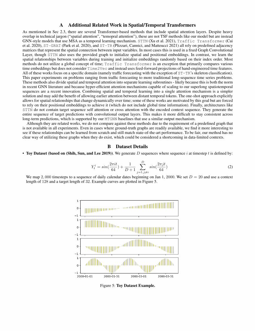
B Dataset Details• Toy Dataset (based on (Shih, Sun, and Lee 2019)). We generate D sequences where sequence i at timestep t is defined by:

Y it = sin(

2πit

64) +

1

D + 1

D∑j=1,j 6=i

sin(2πjt

64) (2)

We map 2, 000 timesteps to a sequence of daily calendar dates beginning on Jan 1, 2000. We set D = 20 and use a contextlength of 128 and a target length of 32. Example curves are plotted in Figure 5.

Figure 5: Toy Dataset Example.

• NY-TX Weather (new). We obtain hourly temperature readings from the ASOS weather network. As described in ourintroductory example, we use three stations located in central Texas and three more located hundreds of miles away in easternNew York. The data covers the years 1949 − 2021, making this a very large dataset by TSF standards. Many of the longestactive stations are airport weather stations. We use the airport codes ACT (Waco, TX), ABI (Abilene, TX), AMA (Amarillo,TX), ALB (Albany, New York) as well as the two largest airports in the New York City metro, LGA and JFK.

• Metr-LA Traffic (Li et al. 2018). A popular benchmark dataset in the GNN literature consisting of traffic measurementsfrom Los Angeles highway sensors at 6-minute intervals over 4 months in 2012. Both the context and target sequence lengthsare set to 12. We use the same train/test splits as (Li et al. 2018).

• AL Solar (Lai et al. 2018). A popular benchmark dataset in the time series literature consisting of solar power productionmeasurements across the state of Alabama in 2006. We use a context length of 168 and a target length of 24.

• Pems-Bay Traffic (Li et al. 2018). Similar to Metr-LA but covering the Bay Area over 6 months in 2017. The context andtarget lengths are 12 and we use the standard train/test split.Normalization and Time Representation. We normalize the values of each variable sequence independently based on

training set statistics. We represent calendar dates by splitting the information into separate year, month, day, hour, minute, andsecond values and then re-scaling each to be ∈ [0, 1]. This works out so that only the year value is unbounded; we divide by thelatest year present in the training set. The reformatted calendar values form the input to the Time2Vec embedding layer. Asa brief aside, the time embedding mechanism of our model could be used in situations where the context and target sequencetimestamps are different for each variable (e.g., they are sampled at different intervals). We do not take advantage of this inour experimental results because it is not relevant to common benchmark datasets and is not applicable to all the baselines weconsider.

C Model Details and HyperparametersC.1 Spacetimeformer DetailsThere is significant empirical work investigating technical improvements to the Transformer architecture and training routine(Huang et al. 2020) (Liu et al. 2020) (Xiong et al. 2020) (Nguyen and Salazar 2019) (Wu et al. 2021b) (Zhou et al. 2020)(Araabi and Monz 2020) (Fan, Grave, and Joulin 2019) (Shen et al. 2020). We incorporate some of these techniques to increaseperformance and hyperparameter robustness while retaining simplicity. A Pre-Norm architecture (Xiong et al. 2020) is used toforego the standard learning rate warmup phase. We also find that replacing LayerNorm with BatchNorm is advantageousin the timeseries domain. (Shen et al. 2020) argue that BatchNorm is more popular in Computer Vision applications becausereduced training variance improves performance over the LayerNorms that are the default in NLP. Our experiments addempirical evidence that this may also be the case in timeseries problems. We also experiment with PowerNorm (Shen et al.2020) and ScaleNorm (Nguyen and Salazar 2019) layers with mixed results. All four variants are included as a configurablehyperparameter in our open-source release.

As mentioned in Sec 3.2, the output of our model is a sequence of parameterized Normal distributions that folds the flattenedspatiotemporal sequence back into its original concatenated format and discards predictions on start tokens. This lets us choosefrom several different loss functions. Most datasets use either Mean Squared Error (MSE) or Mean Absolute Error (MAE) basedsolely on the mean of the output distribution; in these cases the standard deviation outputs are untrained and should be ignored.We occasionally compare Root Relative Squared Error (RRSE) and Mean Absolute Percentage Error (MAPE) - though theyare never used as an objective function. We also consider a Negative Log Likelihood (NLL) loss that maximizes the probabilityof the target sequence according to the output distribution and makes use the model’s uncertainty estimates. An example of theprediction distributions learned by the NLL loss is shown in Figure 6.

Figure 6: Temperature Forecasts with Uncertainty. Spatiotemporal Transformers with NLL loss functions increase predictionuncertainty along the target sequence and at daily low and high temperatures in the NY-TX Weather dataset.

TSF datasets are generally much smaller than their NLP counterparts. As a result, we employ a number of regulariza-tion techniques and tend to prefer narrower architectures than are common in NLP. We add dropout to the embedding layer,

query/key/value layers, feed-forward layers and attention outputs. Inspired by discussion on Transformer training on smallNLP datasets (Dettmers 2020), we also experiment with full token dropout in which entire input tokens are zeroed after theembedding phase - with little success.

Our architecture consists of four types of attention (Fig 3). “Global Self Attention” and “Global Cross Attention” attendto the entire spatiotemporal sequence, while “Local Self Attention” and “Local Cross Attention” attend to the timesteps of asingle variable in isolation. Many Long-Range Transformer architectures include a concept of “local” vs “global” attention.For example, BigBird (Zaheer et al. 2020), Star-Transformer (Guo et al. 2019) and BP-Transformer (Ye et al.2019) connect each token to local tokens in addition to global tokens. In these methods, “local” tokens are adjacent in terms ofsequence order. This aligns well with the assumption that NLP sequences have meaningful order. Our flattened spatiotemporalsequence complicates that assumption because tokens can be adjacent while originating from different variables at vastly dif-ferent timesteps. Regardless, we use the term “local” in a spatial sense where it refers to all timesteps within a single variable.Our local attention is straightforwardly implemented on top of any open-source MSA variant by splitting the spatiotemporalsequence into its separate variables, folding this extra dimension into the batch dimension, performing attention as normal andthen reversing the transformation. The attention mechanism used in all four types is configurable, and our open-source releaseincludes ProbSparse Self Attention (Zhou et al. 2021), Nystromformer Self Attention (Xiong et al. 2021), PerformerSelf/Cross Attention in addition to the standard Self/Cross Full Attention. In practice, the sequence lengths considered in thispaper require Performer Global Attention. The Local Attention modules are much more flexible; we default to Performer forsimplicity.

Table 7 provides an overview of the hyperparameters used in our experiments. The values were determined by a brief sweepbased on validation loss. It is worth reiterating that these models are quite small relative to Informer and tiny in comparison tostandard NLP architectures (Vaswani et al. 2017). The architectures listed in Table 7 consist of 1−3M parameters. The memoryrequirements of our model are a central engineering challenge in this work, but Transformers do scale well with sequence lengthin terms of total parameter count. In contrast, methods like MTGNN grow larger with L and can become significantly larger thanour model in datasets like NY-TX Weather or AL Solar. Temporal-only ablations add an extra encoder and decoder layer tohelp even out the difference in parameter count that comes with skipping local attention modules.

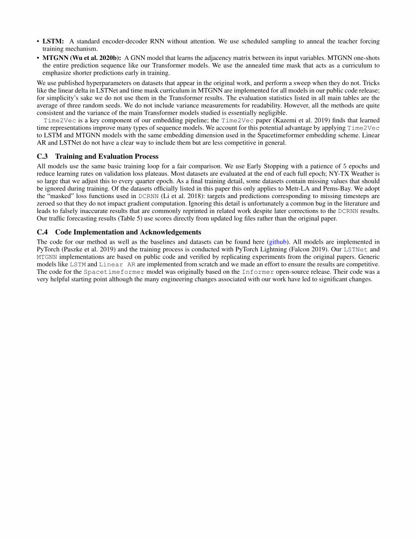
NY-TXWeather AL Solar Metr-LA Pems-Bay Toy

Model Dim 200 128 128 128 100FF Dim 800 512 512 512 400Attn Heads 8 8 8 8 4Enc Layers 2 3 5 4 4Dec Layers 2 3 4 4 4Initial Convs 0 1 0 0 0Inter. Convs 0 0 0 0 0

Local Self Attn performer performer performer performer performerLocal Cross Attn performer performer performer performer performerGlobal Self Attn performer performer performer performer performerGlobal Cross Attn performer performer performer performer performerNormalization batch batch batch batch batchStart Token Len (8, 16, 32) 8 3 3 4Time Emb Dim 12 12 12 12 12

Dropout FF 0.2 0.3 0.3 0.4 .3Dropout Q/K/V 0 0 0 0 0Dropout Token 0 0 0 0 0Dropout Emb 0.1 0.2 0.3 0.3 0L2 Weight 0.01 0.01 0.01 0.01 0

Table 7: Hyperparameters for Spacetimeformer main experiments.

C.2 Baseline DetailsIn addition to variants/ablations of our Transformer framework, we consider several other Deep Learning architectures for TSF:

• Linear AR: A simple autoregressive linear model that acts independently on each input variable.• LSTNet (Lai et al. 2018): A mix of RNN and Conv1D layers with skip connections that predicts the difference between

the final output and the above linear model. The fully autoregressive approach does not scale well with some of the sequencelengths considered in this paper. For this reason, we do not use LSTNet in all experiments.

• LSTM: A standard encoder-decoder RNN without attention. We use scheduled sampling to anneal the teacher forcingtraining mechanism.

• MTGNN (Wu et al. 2020b): A GNN model that learns the adjacency matrix between its input variables. MTGNN one-shotsthe entire prediction sequence like our Transformer models. We use the annealed time mask that acts as a curriculum toemphasize shorter predictions early in training.

We use published hyperparameters on datasets that appear in the original work, and perform a sweep when they do not. Trickslike the linear delta in LSTNet and time mask curriculum in MTGNN are implemented for all models in our public code release;for simplicity’s sake we do not use them in the Transformer results. The evaluation statistics listed in all main tables are theaverage of three random seeds. We do not include variance measurements for readability. However, all the methods are quiteconsistent and the variance of the main Transformer models studied is essentially negligible.Time2Vec is a key component of our embedding pipeline; the Time2Vec paper (Kazemi et al. 2019) finds that learned

time representations improve many types of sequence models. We account for this potential advantage by applying Time2Vecto LSTM and MTGNN models with the same embedding dimension used in the Spacetimeformer embedding scheme. LinearAR and LSTNet do not have a clear way to include them but are less competitive in general.

C.3 Training and Evaluation ProcessAll models use the same basic training loop for a fair comparison. We use Early Stopping with a patience of 5 epochs andreduce learning rates on validation loss plateaus. Most datasets are evaluated at the end of each full epoch; NY-TX Weather isso large that we adjust this to every quarter epoch. As a final training detail, some datasets contain missing values that shouldbe ignored during training. Of the datasets officially listed in this paper this only applies to Metr-LA and Pems-Bay. We adoptthe “masked” loss functions used in DCRNN (Li et al. 2018): targets and predictions corresponding to missing timesteps arezeroed so that they do not impact gradient computation. Ignoring this detail is unfortunately a common bug in the literature andleads to falsely inaccurate results that are commonly reprinted in related work despite later corrections to the DCRNN results.Our traffic forecasting results (Table 5) use scores directly from updated log files rather than the original paper.

C.4 Code Implementation and AcknowledgementsThe code for our method as well as the baselines and datasets can be found here (github). All models are implemented inPyTorch (Paszke et al. 2019) and the training process is conducted with PyTorch Lightning (Falcon 2019). Our LSTNet andMTGNN implementations are based on public code and verified by replicating experiments from the original papers. Genericmodels like LSTM and Linear AR are implemented from scratch and we made an effort to ensure the results are competitive.The code for the Spacetimeformer model was originally based on the Informer open-source release. Their code was avery helpful starting point although the many engineering changes associated with our work have led to significant changes.