SBAC-PAD'99 11th Symposium on Computer Architecture and High Performance Computing- Natal- Brazil 157

LogP Modelling of List Algorithms W. Amme1, P. Braun1, W. Lowe2, andE. Zehendner1

1 FakuiHit flir Mathematik und lnformatik. Friedrich-Schiller-Universitat.

07740 Jena- Germany. E-mail: amme, braunpet, nez@idec02. in f. uni- j ena. de

2 IPD, Universitat Karlsruhe. 76 128 Karlsruhe - Germany.

E-mrul: loewe@ipd.info.uni-karlsruhe.de

Abstract-We presenl lechniques for dislribuling lists for processing on dis­

lribuled and shared mcmory archilectures. The LogP cosi model is ex­lended for evalualing lhe schedules for lhe given problerns and archilec­lures. We consider bolh bounded and unbounded lists. The lheoretical results are confinncd by measurements on a KSR-1.

Keywords- Parallel Lisl Compulations, LogP Model, Runlime Pre­dictions and Measurements

I. INTRODUCTION

Most parallel algorithms operate on arrays because they are easy to distribute and redistribute, particularly, if their size is fixed, (c.f. [9]). However, arrays are not appropriate for a wide range o f problems, e.g. for algorithms on graphs. But the lack of efficient distribution techniques of the ele­ments forces programmers to use arrays instead of lists even i f the latter is a better choice from a designer's point of view. The problem is even worse for the parallelization of sequen­tial c ode, as the programmer usually does not consider parai­lei execution.

The obvious solution, which would be the list converted into an array before distribution, is too wasteful in memory. As shown below, it is also a bad choice w.r.t. the required time. Matsumoto, Han and Tsuda [8) proposed to collect only the addresses of list elements in an array and distribute this array. This saves memory if the element's size exceeds the size of an address. However, it only works for (virtual) shared memory systems. To decide whether it is more effi­cient than the former solution, we have to compare costs for local and non-local copy operations. The costs depend on the size o f the data.

In general, to compare the different strategies for distribu­tion, a cost model is required which would reftect the time for searching a list compared to the time for computation on the elements. Additionally, latency, overhead, and band­width for communication should be considered. The LogP­machine [2] is a generic machine model reftecting the com­munication costs with parameters Latency, overhead, and gap (which is actually the inverse of the bandwidth). The number o f processors are described by parameter P. The pa-

rameters have been determined for severa) parallel computers [2, 3, 6, 4]. These works confirmed ali LogP-based runtime predictions.

In a virtual shared memory machine, access to non-local objects is done by data transfer via a communication net­work. Of course, there is a Latency between initiating the access and receiving the object. Initiating and receiving may be two separa te operations that cause overhead on the proces­sors. Between both operations, computations are possible. A gap between two succeeding memory accesses must be guar­anteed due to bandwidth limitations. Hence, virtual shared memory architectures are also covered by the LogP model.

With lhe cost model, we may predict lhe quality of each distribution technique in lerms o f the required execution time on a specific target machine. This paper is restricted to ap­plications where the parallel computations on the single list elements are independent of each other, analyzed e.g. by techniques of [I). Dueto this restriction, our approach may achieve better results than a general solution, confronted with the same situation. The proposed algorithm is not intended to replace general techniques, but to complete them.

The paper is organized as follows: In section 2, we define the cost model. In section 3, we introduce the distribution algorithms. Section 4 compares the approaches w.r.t. exe­cution times within the cost model. Section 5 confirms the results by measurements. Finally, we conclude our results and show directions o f further work.

li. THE COST MODEL

The LogP cost model reftects communication costs but ig­nores computation times. However, since communication times are given in terms of machine cycles, these costs are comparable with execution times on the processors. In ad­dition to the machine dependent parameters L, o, and g, we assume two further parameters:

• e · n defines the (maximum) costs for searching the list o f size n on the processors o f our parallel machine, and

158 SBAC-PAD'99 11th Symposium on Computer Architecture and High Performance Computing- Natal- Brazi/

• k · n denote the (maximum) costs for computations on n list elements.

Note that the Jatter depends on both, the processor architec­ture and the concrete algorithm. However, ali parameters are easily computable at compile time and may therefore be used for optimization.

Sending (receiving) a message in a distributed memory system or iniliating a far access in a shared memory sys­tem costs time o (overhead) on the processor. A processor can not send (receive) two messages and simultaneously ini­tiate two far accesses, rcspectively, within time g, but may perform other operation immediately after a scnd (receive) and load or pre-fetch (store) operation, rcspcctively. In a dis­tributed memory system, the time between the end o f sending a message and the start o f receiving this message is defined as latency L. In a shared memory system, L denotes the time between the end of the initiation of a far access and the time the date is actually transfered.

If the sending processor is still busy with sending the last bytes of a message while the receiving processor is already busy with receiving, the send and the receive overhead for this message overlap. This happens on many systems, espe­cially for long messages. Modeling this effect as a negative value for the latency avoids the distinction of cases in further calculations.

The time for communication depends on the amount of transfered data. This is not covered by the original LogP­machine model but considered e.g. in [4] where L , o, g are functions of the message size instead of constants. This pa­per uses L(s) , o(s), and g(s), respectively, to denote the la­tency, overhead, and gap, respectively, for data transfers of size s. A single (indivisible) item is of size 1. L(O), o(O), and g(O) denote the cost for data of size zero. That include cost for function calls, etc. The observation from practice is that L(s), o(s), and g(s) may b~ nicely approximated by linear functions. We write max( o, g) ( s) for max( o( s) , g( s)) which is, by assumption, also a linear function.

Example 1 For parsytec's PowerXplorer we measured the values of L(s), o(s), and g(s) for a wide range of sizes s. We approximatedfollowingfunctions: g(s) = 117 + 1.43 · s, o(s) = 70 + s , and L(s) = - 0.82 · s. These approximations have been confinned by comparing predicted and measured execution times [4/.

lll. DISTRIBUTION STRATEGIES

For the parallel processing of a linear list, it is necessary to map the set of Joop iterations into the set of available processors. There are well-known scheduling methods for loops, which are exclusively based on scalar variables or ar­ray operands. Unfortunately these methods cannot be ap­plied when para\Jelizing algorithm using linear lists, as the

iteration space often must be known at compile time. Fur­ther, when using these methods we must be able to access ali neccssary dates in constant time. For linear lists these two demands are obviously not fulfilled.

Essentially, when the list length is known, distribution strategies for linear lists work in two phases:

I . The list elements must be assigned to the processors. 2. A parallel execution o f the list is then performed.

For shared memory architectures, it is sufficient to assign the addresses to the processors. The actual data transfer is au­tomatically performed i f accesses to the addresses occur. In a distributed memory system, the list elements themselves must be distributed.

As already mentioned, Matsumoto, Han and Tsuda [8] of­fer an approach for shared memory systems that-after de­termination of the list Jength-stores the address of each list element in an array. This array is scheduled vertically to the processor set and then processed in parallcl. Analogously on distributed memory systems, we may store the list e lements in an array instead of their addresses. We ca\J this method vectorization or vector method.

Vectorization takes additional memory o f size c* n, where c denotes the size of an address (for shared memory ma­chines) and the size of a list e lement (for distributed mem­ory machines), respectively. This size may be reduced to the maximum size of data transfered to a single processor. For distributed memory architectures, this is a constant part of n, and for shared memory machines, it is even reduced to P. The former reduction is easily obtained by interleaving the copy and the distribute operations. The reduction to P is achieved as follows: We collect the entry elements l; o f a list in an array l. An entry element l; is an anchor of the Jist's portion that is to compute on processor i. Clearly, lll = P. Determination of the entry elements can be performed by a simple list crossing. In a second phase, each processor i bc­gins working on the list item which corresponds to l;. The processar stops when it reaches li+t or the last element. We call this approach list method.

In comparison to the classification above, we distinguish step-by-step methods from pipeline methods. In the former case, distribution and computation are done step by step. Ob­viously, each processor should work on at most m = r f; l elements sequentially to guarantee Joad balancing. In the pipeline method, the processors may start working immedi­ately after they received their portion o f the list.

Since the distribution of the elements and addresses, re­spectively, is not completed for ali processors at the same time, uniform distribution does not guarantee load balancing. This problem is discussed in the subsections and .

SBAC-PAD'99 1 lth Symposium on·Computer Architecture and High Performance Computing - Natal- Brazil 159

Time

Fig. I. Sequential distribution of array elements

IV. A NALYZ ING THE COSTS

This scction compares the time for cxecution for the d if­ferent distribution strategies w.r.l. the cost model from sec­tion II. The first two subsections consider distributed mem­ory machincs. The ncxt subsection describes necessary mod­ifications to apply the results to shared memory machines. The final subsection discusses the results and extends them to the case where n is not known at compile time.

A. Step-by-Step Method

First we analyze the step-by-step method using vectoriza­tion. Collecting n list elements in an array takes time e · n . Thereafter, blocks of size m = f~ 1 must be distributed to the processors. Figure 1 sketches the distribution algorithm.

Lemma 1 Sequential distribution of an array of size n is (upper-) bounded by

tseq(n) = (P- 2) · max(o,g)(m) + L (m) + 2o(m).

Proof' P - 1 blocks of size m must be sent sequen­tially. The last block leaves the source processor at time (P- 2) · max(o(m) , g(m)) + o(m). Transmission requires time L(m). The last processor requires time o for receiving ~m~~- o

However, this is not always the best choice. Consider the following algorithm for distribution, a binary tree tech­nique which may outperform the sequential distribution: The source processor possesses the complete array. If a processor

Fig. 2. Tree distribution of array elements

P; possesses an array equal in size to or smaller than m , it starts computation. Otherwise, P; keeps m array elements and sends the remainder of the array to two other processors Pf and P[, neither o f which possess an array yet. P; sends half of the array to Pf and the other half to P[. Figure 2 sketches this distribution algorithm.

Lemma 2 The tree distribution of an array of size n is (upper-) bounded by

ttree(n) = llogPJ · n 1

(max(o,g)('2(1- p)) + n 1

L('2(1 - p)) + n 1

2o( 2 (1 - p) )).

Proof' We consider the longest path in the broadcast tree. Its depth is l log P J. Ignoring the m items remaining on the pro­cessors, each P; sends half of its array to the two following processors. The i -th send operation on the longest path sends s; = F data items. It requires at most

t ; = max(o, g)(s;) + L(s;) + 2o(s;)

by the same reasoning as in lemma 1 (set P = 3 to see this). By using the linearity of max(o,g)(s) , L(s) , and o(s), and iterating i from 1 to llog P J, the proof is completed. o

It is not possible to guarantee that either algorithm offers better results in ali situations. For small array sizes, the tree

160 SBAC-PAD'99 11th Symposium on Computer Architecture and High Performance Computing- Natal- Brazil

distribution outperfonns the sequential, for small numbers of processors, the opposite is true. We therefore combine both algorithms such that the sequential algorithm starts to distribute the array to p $ P - 1 processors sequentially. Each of the p processors obtains ~ array elements. Then these elements are further distributed by the tree technique to maximal numbers of llog(f P;pl + l )J processors.

Lemma 3 The combined (sequential-tree-) distribution of the datais (upper-) bounded by

n n n t comb = (p- 2) · max(o, g)(-) +L(-)+ 2o(-) +

p p p

llog(fp- pl + 1)J · p

n 1 (max(o, g)(

2P (1 - p)) +

n 1 L( 2P(l - p)) +

n 1 2o(

2p(1- p))).

Proof-Sketch: Correctness follows immediately from the Jemmas 1 and 2. o

Now we choose a value for p, such that t comb is minimal. This depends, o f course, on the LogP parameters and may be easily computed for concrete architectures.

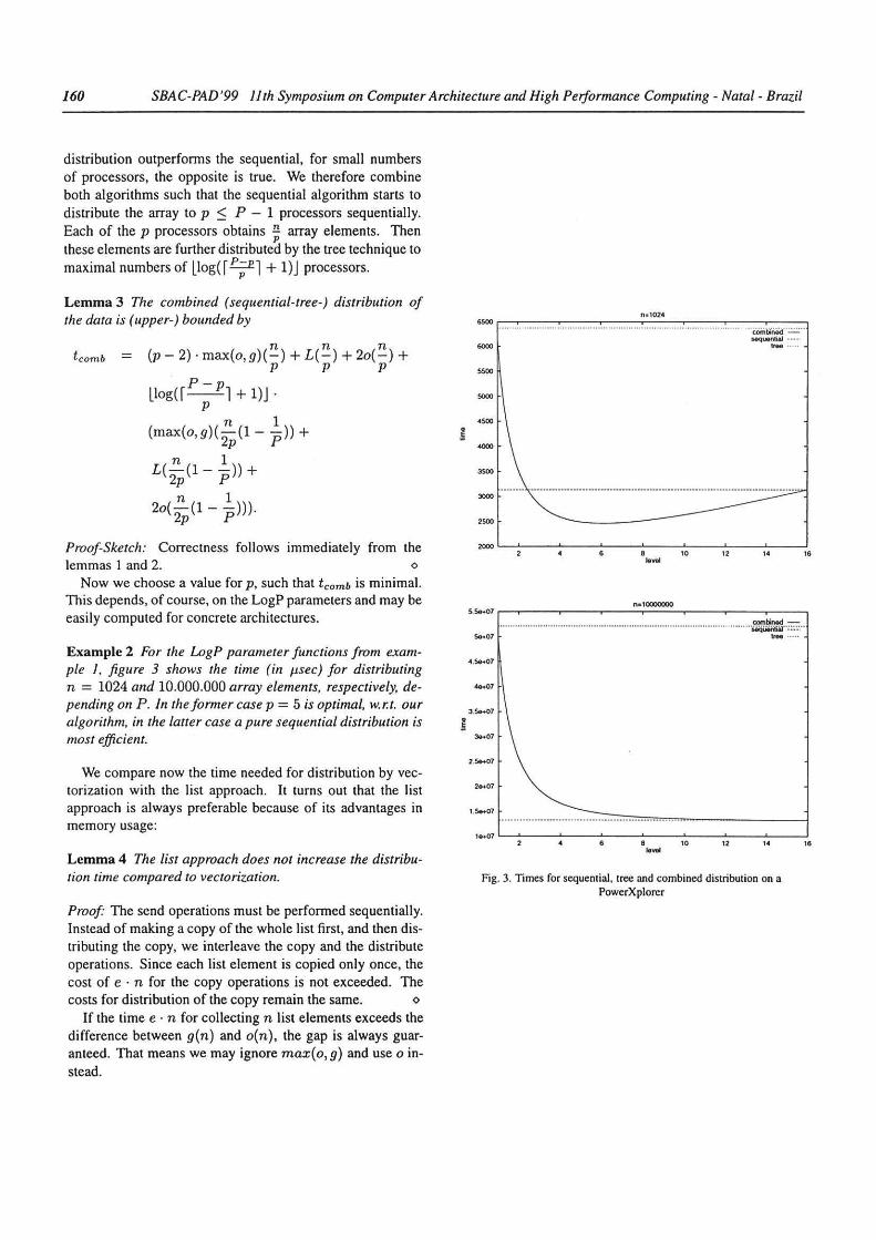
Example 2 For the LogP parameter functions from exam­ple 1. figure 3 shows the time (in Jl.Sec) for distributing n = 1024 and 10.000.000 array elements, respectively, de­pending on P. Jn the former case p = 5 is optimal, w.r.t. ou r algorithm, in the latter case apure sequellfial distribution is most efficient.

We compare now the time needed for distribution by vec­torization with the list approach. It turns out that the list approach is always preferable because of its advantages in memory usage:

Lemma 4 The list approach does not increase the distribu­tion time compared to vectorization.

Proof' The send operations must be perfonned sequentially. lnstead o f making a copy o f the whole list first, and then dis­tributing the copy, we interleave the copy and the distribute operations. Since each list element is copied only once, the cost of e · n for the copy operations is not exceeded. The costs for distribution o f the copy remain the same. o

If the time e · n for collecting n list elements exceeds the difference between g(n) and o(n), the gap is always guar­anteed. That means we may ignore max(o, g) and use o in­stead.

j

R• 1024 ·~r-~--~----~--~~--~----r----r--~

ssoo

''Ci:im~··:..:.:.:.:··

sequential . . .. lrae ·····

roooL-~--~----~--~~--~----~--~--~ 6 8 10 12 14 16

lowl

n• SOOOOOOO

"""l>nod-.................................. ..................................... ............................ ~ .. ,""" Se-+07 liM ···· ·

3.S..07

2.S..07

1.S..07 ........... . . • . . . .....•........ ::: .. ::-: .•. :::-... ::: .. ::: ... ::-:c ... ::-: .. ,., ... = .. ·=--~-- - - - ----l 1-7 L-~-~--~-~a--~,o~-~,~2 -~,~. -~,e

lowl

Fig. 3. Times for sequential, tree and combined distribution on a PowerXplorer

SBAC-PAD'99 11th Symposium on Computer Architecture and High Performance Computing- Natal- Brazil 161

Note that for some LogP parameter functions, the com­bined algorithm is always faster then the pure sequential al­gorithm even if the size of the array approaches infinityl . However, these parameter functions describe only artificial architectures since both L and o must be constants, while g must increase with the size o f the data transfer. Therefore, we assume that for existing parallel machines, the pure sequen­tial distribution is the fastest for sufficiently large array sizcs n. This means that for sufficiently large n, it is adequate to describe the costs of distribution by the (linear) function t seq instead of tcomb·

The following theorem merges the results from this sub­section:

Theorem 5 Using the step-by-step approach, parai/e/ com­putation o f a list with n elements is ( upper-) bounded by

tstep-by-step (n) n = t se9 (n)+e·n+k·(p+1),

which is a linear function in n.

Proof Becausc of lemma I and the time e · n for copying n list elements, distribution o f the list takes time tseq ( n) + e · n. Each processar works sequentially on r~ l elemcnts, which explains the term ( ~ + 1) · n as an upper boundary for computations. t 5 .,9 (n) as well as e· n and k · ( .p + 1) are linear functions. Therefore, t step- by-step(n) is linear. o

B. Pipeline Methods

We use the sequentiallist approach to distribute the list el­ements according to the pipeline method. The question is: how many list elements should each processar get to guaran­tee that no unnecessary idle times occur? Let t; be the time for collecting the list elements dedicated to processar p; plus the costs for the corresponding send operation, 1 ~ i < P . Because of the observations from the last subsection, t; is defined by the following recurrence:

t1 = o(nl) + e · n1 ,

t ; t;-1 + o(n;) +e· n; ,

(I)

(2)

where n; is the amount of data sent to processar p;. T; de­notes the time processar p; needs to complete computations. Processar pp is the source processar (the processar that pos­sesses the originallist): We set tp = tp_ 1 • The source pro­cessar may start its computations if ali messages have been sent. Obviously, it holds that

Tp = tp_ l + k · np, (3)

T; = t; + o(n;) + L(n;) + k · n;, (4)

1To see this, compute a ditferentiation of tcomb with respect to p. For some values o f the LogP parameter functions, this derivative is zero for I < p < P which is a minimum for tcomb· Maple does most ofthejob.

To avoid idle times on the processar, we solve the following linear equation system:

T; = T;+l, 1 ~ i ~ P, (5) p

n = :Ln;. (6) i= l

Let o(s) = oo+o·s and L(s) = Lo+L·s. The linearequation system may be expressed symbolically as 1 ~ i ~ P - 2 by transforming the equations above.

T; = T;+1

t; + o(n;) + L(n;) + kn; = ti+l + o(n;+I) + L(ni+d + kni+l

t; + o(n;) + L(n;) + kn; = t; + 2o(ni+I) + eni+l + L(ni+I) + kn;+l

o(n;) + L(n;) + kn;

2o(n;+I) + eni+l + L(ni+i) + kni+1 =

(o+ L+ k)n; - (2o +L+ e + k)n;+1 = oo

By similar transformations we obtain

TP-1

(o+ L+ k)nP- 1 - (o + L+ k)np

= Tp

o We sctm1 = o+L+kandm2 = -(2o+L+e+k). The general linear equation system for arbitrary LogP parameters is defined by

ffi) m2 o o o o oo o m1 m2 o o o oo o o ml m2 o o o o

ii=

o o o o m2 o o o o o o o m1 m2 o 1 1 1 1 1 1 n

where the matrix is squared with P rows and columns. The i-th row, 1 ~ i < P- 1, represents the equations o f the form T; = Ti+ 1 (note the special case for i = P - 1). The last row represents equation (6). The solution is real valued for n 1 · · · np. We must round it out such that n = "L::1 n ; still holds.

Theorem 6 Using the pipeline approach, para/lei computa­tion o f a list with n elements is ( upper-) bounded by

tpipe(n) = (o+ e)* n + (P- 1) * 0o + (k- o- e)* (np + 1),

which is a Linear function in n.

162 SBAC-PAD'99 11th Symposium on Computer Architecture and High Performance Computing- Natal- Brazil

ProofSketch: For the execution time tpipe(n) it holds that

Easy substitutions for Tp using equations (I) to (6) complete the correctness proof. To note that tpipe ( n) is linear, observe that np is a constant portion of n depending on the LogP parameters. o

C. Shared Memory Machines

For shared memory systems, the cost function for the data transfer differs slightly. For our purpose it is sufficient to consider load or pre-fetch operations to non-local data. Such an opcration takes time o on the processor. L time units !ater, the data is available locally; the next load or pre-fetch must guarantce time g. However, i f the transpor! o f data from non­local to local memory may not be divided from the load oper­ation (e.g. no pre-fctch operation exists), this differentiation is worth nothing. We have to consider far accesses as an in­divisible function. In the latter case, wc may integrate these costs into the costs k for the computations on thc list.

In the step-by-stcp method, r n · PP 11 elements must be considered for the determination of the entry elements. Af­terwards, ali processors execute r~ l elements in parallel. Ahogether, this results in costs:

tstep-by-step ( n) P-1 n

e · (n · - - + 1) + k · (- + 1) p p .

For the pipeline method, the quota o f the list for each pro­cessar can be calculated by solving a linear equation system. Ali processors should stop their work at the same time. We set m = ~ and obtain, by similar computations as in the last subsection:

-m m+1 o o o o -m 1 m+1 o o o

ii=

-m 1 1 1 1 m+1 o 1 1 1 1 1 2 n

Example 3 Table I shows the proportional distribution of the list to four processors for different cost re/ations m.

The costs for executing the whole list can be determined by n1.

tpipe (n) (n1 + 1) · (e+ k).

D. Discussion

The pipeline method is always fas ter then the step-by-step method, if P > 1 and communication is not ' free' . This is obvious as idle times between receiving the data and starting computations is saved, while load balancing is guaranteed.

TABLEI

PROPORTIONAL DISTRIBUTION OF A LINEAR .

m

I 50.00 25.00 12.50 12.50 2 39.13 26.09 17.39 17.39 3 34.78 26.09 19.57 19.57 4 32.47 25.97 20.78 20.78 5 31.03 25.86 21.55 21.55 lO 28.07 25.52 23.20 23.20 50 25.62 25.12 24.63 24.63 100 25.31 25.06 24.81 24.81 250 25.12 25.02 24.93 24.93

We assumed that n is known in advance. If only upper bounds for n are statically known, the (upper) time bounds are still guaranteed since they are monotonely increasing with n. Now we drop this assumption and claim that N is a random variable with expectation n = E[N].

Theorem 7 Let T step-by-step(n) and Tpipe(n) be random variables for the time required for computation on lists with expected length n using the step-by-step and the pipeline methods, respectively. For these expectations it holds that

tstep-by-step ( n)

tpipe(n)

= E [Tstep-by-step(n)J,and

E [Tpipe (n)J.

Proof" tstep-by-step(n) and tpipe(n) are linear in n, see the­orems 5 and 6. Because of the linearity of the expectation operator, the theorem holds. <>

When the number o f list items is unknown and its variance is too large, the list length may also be quantified by a com­plete list crossing at runtime. The calculation of the last sub­sections then occur also at runtime. This is not too expensive because the linear equation systems give a percentage of the list length n schcduled to each processor, i f n is variable. We should only count the additional costs for the list crossing. Obviously, the described methods are easily extendable to any linear cost function for communication of list elements and succeeding parallel computations.

V. MEASUREMENTS

Ali methods have been implemented on a KSR-1 system [7] with eight processors, each with eight MByte local mem­ory. The KSR-1 is a virtual-shared-memory-system, i.e., each processar has its own local memory, but there is only one global address space. Every memory cell can be ac­cessed by every processar through a communication network called ALLCACHE-engine.

SBAC-PAD '99. 11th Symposium on Computer Architecture and High Performance Computing- Natal- Brazil 163

80000

70000

60000

50000

30000

20000

10000

b t ·S1ep­ill-ppo - ­

Y«f:Of • S1ep ·O·· YedOf • pipe X

KSR-Tmaa

n

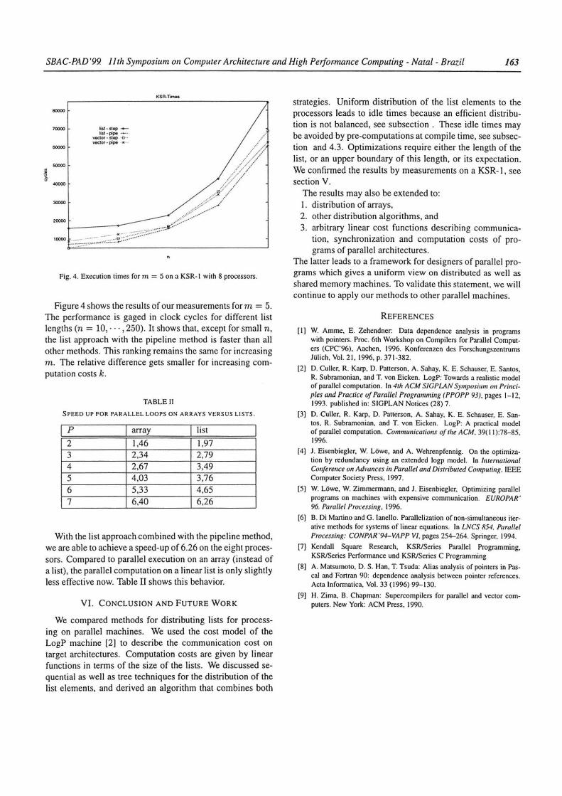
Fig. 4. Execulion times for m = 5 on a KSR- 1 w ith 8 processors.

Figure 4 shows the results o f ou r measurements for m = 5. The performance is gaged in clock cyclcs for different list lengths (n = 10, - - -, 250). It shows that, except for small n, the list approach with the pipeline method is faster than ali other methods. This ranking remains the same for increasing m. The relative difference gets smaller for increasing com­putation costs k.

TABLE 11

SPEED UP FOR PARALLEL LOOPS ON AR RAYS VERSUS LI STS.

IP I array I list

2 1,46 1,97 3 2,34 2,79 4 2,67 3,49 5 4,03 3,76

6 5,33 4,65 7 6,40 6,26

With the list approach combined with the pipeline mcthod, we are able to achieve a speed-up o f 6.26 on the eight proces­sors. Compared to parallel execution on an array (instead of a list), the parallel computation on a linear list is only slightly less effective now. Table 11 shows this behavior.

VI. CONCLUSION AND FUTURE WORK

We compared methods for distributing lists for process­ing on parallel machines. We used the cost model of the LogP machine [2] to describe the communication cost on target architectures. Computation costs are given by linear functions in terms of the size of the lists. We discussed se­quential as well as tree techniques for the distribution of the list elements, and derived an algorithm that combines both

strategies. Uniform distribution of the list elements to the processors leads to idle times because an efficient distribu­tion is not balanced, see subsection . These idle times may be avoided by pre-computations at compile time, see subsec­tion and 4.3. Optimizations require either the length of the list, or an upper boundary of this length, or its expectation. We confirmed the results by measurements on a KSR-1 , see section V.

The results may also be extended to: I. distribution of arrays, 2. other distribution algorithms, and 3. arbitrary linear cost functions describing communica­

tion, synchronization and computation costs of pro­grams of parallel architectures.

The latter leads to a framework for designers o f parallel pro­grams which gives a uniform view on distributed as well as shared memory machines. To validate this statement, we will continue to apply ou r methods to other parallel machines.

REFERENCES

[I) W. Amme, E. Zehendner: Data dependenee analysis in programs with pointers. Proc. 6th Workshop on Compilers for Parallel Comput­ers (CPC'96), Aachen, 1996. Konferenzen des Forschungszentrums Jülich. Vol. 2 1, 1996. p. 37 1-382.

[21 D. Culler, R. Karp, D. Pallerson, A. Sahay. K. E. Schauser. E. Santos, R. Subramonian. and T. von Eicken. LogP: Towards a realistic model of parallel computation. In 4th ACM SJGPU\N Symposiwn on Princi­plu cmd Practice of Parai/e/ Programming (PPOPP 93), pages 1-12. 1993. published in: S IGPLAN Nolices (28) 7.

(3) D. Culler, R. Karp, D. Pauerson. A. Sahay, K. E . Schauser. E. San­tos. R. Subramonian, and T. von Eicke n. LogP: A practical model of parallel computation. Communications of the ACM. 39( li ):78-85, 1996.

[4] J. Eisenbiegler, W. Lowe, and A. Wehrenpfennig. On the optimiza­tion by redundancy using an extended logp model. In lntem ational Conferena on Advances in Parai/e/ and Di.ttributed Compllling. IEEE Computcr Society Press, 1997.

[5] W. Lowe, W Zimmermann. and J. Eisenbicgler. Optimizing parallel programs on machines with expensive communicalion. EUROPAR' 96. Parai/e/ Processing, 1996.

[6] B. Di Martino and G. lancllo. Parallelization of non-simultaneous iter­alive methods for systems of linear cquations. In LNCS 854. Parai/e/ Processing: CONPAR'94-VAPP VI, pages 254-264. Springcr. 1994.

[7] Kendall Square Rescarch, KSR/Series Parallel Programming, KSR!Series Performance und KSR/Series C Programming

[8] A. Matsumoto, D. S. Han, T. Tsuda: Alias analysis of pointers in Pas­cal and Fon ran 90: dependence analysis between pointcr references. Acta lnformatica. Vol. 33 (1996) 99- 130.

[9] H. Zima, B. Chapman: Supercompilers for parallel and vector com­puters. New York: ACM Press, 1990.