Logistic Control In Automated Transportation Networks - Universiteit

Logistic Control In Automated Transportation Networks

Mark Ebben

2001

Ph.D. thesisUniversity of Twente

Also available in print:www.tup.utwente.nl/uk/catalogue/management/logistic-control

T w e n t e U n i v e r s i t y P r e s s

http://www.tup.utwente.nl/uk/catalogue/management/logistic-control

Logistic Control in Automated Transportation Networks

This thesis is number D-40 of the thesis series of the Beta Research School for OperationsManagement and Logistics. The Beta Research School is a joint effort of the departmentsof Technology Management, and Mathematics and Computing Science at the TechnischeUniversiteit Eindhoven and the Centre for Production, Logistics and OperationsManagement at the University of Twente. Beta is the largest research centre in theNetherlands in the field of operations management in technology-intensive environments.The mission of Beta is to carry out fundamental and applied research on the analysis,design and control of operational processes.

Dissertation committeeChairman / secretary Prof.dr. W. van RossumPromotor Prof.dr. A. van HartenAssistant Promotor Dr. M.C. van der HeijdenMembers Prof.dr.ir. W.M.P. van der Aalst (Technische Universiteit Eindhoven)

Prof.dr.ir. M.B.M. de Koster (Erasmus Universiteit Rotterdam)Prof.dr.ir. M.F.A.M. van MaarseveenProf.dr. R.A. StegweeDr.ir. A. Verbraeck (Technische Universiteit Delft)Prof.dr. W.H.M. Zijm

AcknowledgementHerewith we express our gratitude to Connekt (the Dutch knowledge centre for traffic andtransport) for their funding of the simulation study that was the basis of our research results.Connekt coordinates a project for the pre-design of an underground logistic system aroundAmsterdam Airport Schiphol, which was used as a case study in this thesis.

Publisher: Twente University PressP.O. Box 217, 7500 AE Enschede, the Netherlandswww.tup.utwente.nl

Cover design: Hana Vinduška, EnschedeEnglish correction: Lorraine van Dam, DelftPrint: Grafisch Centrum Twente, Enschede

© M.J.R. Ebben, Enschede, 2001No part of this work may be reproduced by print, photocopy or any other means without thepermission in writing from the publisher.

ISBN 9036515912

LOGISTIC CONTROL INAUTOMATED

TRANSPORTATION NETWORKS

PROEFSCHRIFT

ter verkrijging vande graad van doctor aan de Universiteit Twente,

op gezag van de rector magnificus,prof.dr. F.A. van Vught,

volgens besluit van het College voor Promotiesin het openbaar te verdedigen

op vrijdag 8 juni 2001 te 16.45 uur

door

Mark Jacobus Richard Ebbengeboren op 5 juli 1973

te Wierden

Dit proefschrift is goedgekeurd door de promotor

prof.dr. A. van Harten

en de assistent-promotor

dr. M.C. van der Heijden

i

��

This thesis is the result of several years of research. It could not have beencompleted without the help of many others. A lot of people contributed to the finalresult, by in-depth discussions, interesting ideas, mental support, jokes or coffee.Therefore, I would like to thank several people for their contribution.First of all I want to thank my supervisors Aart van Harten and Matthieu van derHeijden, both for the fruitful discussions about the research and the pleasantcooperation within the OLS-project. Furthermore, I enjoyed working together withNoud Gademann and Durk-Jouke van der Zee, discussing specific research topicsand writing papers.Speaking about the OLS-project. This project provided an environment withmultiple disciplines, in which a lot of enthusiastic people worked on the latesttechnological developments. I want to thank Connekt, one of the initiators of theOLS-project, for their funding of the simulation study that was the basis of ourresearch results. It was fun working on such an interesting project. I want to thankall participants in the OLS-project for the pleasant cooperation, in particular thesimulation group at Delft University of Technology, Alexander Verbraeck, YvoSaanen and Edwin Valentin. I would also like to thank the students, Marc Bakhuis,Marcel Brinkman and Gerben Verstegen, whose work contributed to the completionof this thesis.Besides work there are also other things. I want to thank my colleagues of theOMST department for the pleasant atmosphere and relaxing coffee breaks. In thelast period of writing it was of great help to meet PhD students in the same phase ofwriting. They understand the pressure and obstacles in these last months. EspeciallyI want to mention Frank de Bakker. We both worked many evenings on the lastdetails of our theses, but there was still time for diner or coffee to discuss also otherthings than research.Last but certainly not least, I want to thank family and friends for their interest in myresearch, and even more for the pleasant and enjoyable holidays, trips, weekends,etc.

THANKS!

Enschede, April 2001

Mark Ebben

iii

��

��

��

� ��

1.1 MOTIVATION ...............................................................................................11.1.1. Need for innovative transport and logistic concepts...........................11.1.2. Dealing with congestion .....................................................................21.1.3. Underground freight transportation ...................................................31.1.4. Research motive ..................................................................................5

1.2 RESEARCH DESIGN.......................................................................................61.2.1. Research setting ..................................................................................61.2.2. Research objectives and research questions.......................................71.2.3. Demarcation and assumptions..........................................................101.2.4. Research approach ...........................................................................11

1.3 POSITIONING THE RESEARCH PROBLEM AND OUR CONTRIBUTIONS ............131.3.1. Logistic modeling..............................................................................131.3.2. Physical system design......................................................................141.3.3. Planning and control ........................................................................16

1.4 THESIS OUTLINE ........................................................................................21

� �� !��"��#$��%�#��"��#��!��&�#��"��'

2.1 INTRODUCTION ..........................................................................................232.2 OBJECT ORIENTED ANALYSIS AND DESIGN.................................................242.3 PHYSICAL PROCESSES AND PHYSICAL OBJECTS..........................................27

2.3.1. Process description...........................................................................272.3.2. Basic objects and inheritance structure............................................292.3.3. Object hierarchy (“part of”, aggregation) .......................................332.3.4. Class diagrams..................................................................................34

2.4 CONTROL STRUCTURE ...............................................................................36

iv

2.4.1. Primary process control....................................................................372.4.2. Secondary process control ................................................................40

2.5 DESIGN OF THE CONTROL OBJECTS ............................................................402.6 INFORMATION STRUCTURE AND INFORMATION OBJECTS............................45

2.6.1. Information exchange and communication lines ..............................462.6.2. Performance information..................................................................50

2.7 SUMMARY .................................................................................................51

' ��(�#��!��)'

3.1 INTRODUCTION ..........................................................................................533.2 PROJECT STRUCTURE .................................................................................54

3.2.1. Feasibility study ................................................................................543.2.2. Definition study.................................................................................543.2.3. Pre-design phase...............................................................................55

3.3 SUB-PROJECT TRANSPORTATION AND CONTROL TECHNOLOGY..................563.3.1. System design....................................................................................563.3.2. Functional requirements ...................................................................593.3.3. Vehicles.............................................................................................603.3.4. Terminal and dock design.................................................................613.3.5. Operating and information system....................................................643.3.6. Simulation .........................................................................................653.3.7. Connekt Test Site...............................................................................67

3.4 MODEL INPUT: TRANSPORTATION FLOWS ..................................................683.5 OPTIMIZATION VERSUS SIMULATION: ESTIMATION OF THE RESOURCE

REQUIREMENTS ...........................................................................................733.5.1. An analytical model ..........................................................................733.5.2. Example: Stommeer layout ...............................................................783.5.3. Resource requirements for the 3 different layouts ............................80

3.6 CONCLUSIONS............................................................................................81

* ��#��!��$��(+�#��!��"�!��,'

4.1 INTRODUCTION ..........................................................................................834.2 MODEL AND ASSUMPTIONS........................................................................84

4.2.1. Integer linear programming formulation..........................................854.2.2. Dynamic programming formulation .................................................874.2.3. The difficulties of vehicle management and the available

information........................................................................................894.3 LITERATURE ..............................................................................................914.4 HEURISTICS FOR EMPTY VEHICLE MANAGEMENT.....................................92

4.4.1. Local coordination using dispatching rules (EVM1 and EVM2)......934.4.2. Hierarchical coordination (EVM3)...................................................95

4.5 INTEGRATED PLANNING (EVM4)...............................................................974.6 LOGISTICS QUEUING NETWORK (EVM5) ................................................101

v

4.6.1. Reformulating the ILP model..........................................................1034.6.2. Calculating the gradients................................................................1074.6.3. Calculating the upper bounds .........................................................1084.6.4. Summary of the LQN algorithm......................................................1104.6.5. Application of the LQN algorithm ..................................................1124.6.6. Modifications of the LQN algorithm...............................................1134.6.7. Drawbacks of the LQN algorithm with possible solutions..............114

4.7 NUMERICAL INVESTIGATION....................................................................1154.7.1. Experimental setting .......................................................................1154.7.2. Initial experiments ..........................................................................1164.7.3. Numerical results ............................................................................120

4.8 CONCLUSIONS..........................................................................................123

) ��-(�.�/.�$��-��)

5.1 INTRODUCTION ........................................................................................1255.2 LITERATURE REVIEW ...............................................................................128

5.2.1. Traffic literature..............................................................................1285.2.2. Queuing models ..............................................................................1295.2.3. Machine scheduling ........................................................................130

5.3 CONTROL RULE CONCEPTS.......................................................................1315.3.1. Assumptions and notation ...............................................................1315.3.2. Characterization of control rules....................................................131

5.4 PERIODIC CONTROL .................................................................................1335.4.1. Introduction and assumptions.........................................................1335.4.2. Stability conditions..........................................................................1365.4.3. Waiting times if the succession time is negligible (δ=0).................1365.4.4. Numerical results for δ = 0.............................................................1395.4.5. Waiting times in the case of strictly positive succession time

(δ > 0) .............................................................................................1405.4.6. Numerical experiments for δ > 0 ....................................................1475.4.7. Generalization to compound Poisson arrivals................................151

5.5 ADAPTIVE CONTROL RULES .....................................................................1515.5.1. Adaptive local control.....................................................................1525.5.2. Adaptive look-ahead control...........................................................1535.5.3. Dynamic programming ...................................................................155

5.6 DESIGN OF THE SIMULATION STUDY ........................................................1575.7 ANALYSIS OF SIMULATION RESULTS ........................................................158

5.7.1. Default settings ...............................................................................1585.7.2. Alternative system configurations ...................................................1595.7.3. Sensitivity for the information horizon and planning frequency.....1615.7.4. Practical use of the DP-approach ..................................................1625.7.5. AGV length and safety precautions.................................................162

5.8 A TWO-WAY TRACK IN A CLOSED SYSTEM ...............................................1635.8.1. The effects of convoys on the system ...............................................163

vi

5.8.2. Numerical results for the OLS-case ................................................1665.9 CONCLUSIONS..........................................................................................167

0 ��$��$��!��"�!��%��#��"��01

6.1 INTRODUCTION ........................................................................................1696.2 BATTERY MANAGEMENT .........................................................................170

6.2.1. Introduction ....................................................................................1706.2.2. Implications of battery constraints for the logistic control .............1716.2.3. Logistic performance in case of battery constraints .......................1776.2.4. Structure for a cost trade-off...........................................................1806.2.5. Conclusions.....................................................................................182

6.3 FAILURE MANAGEMENT...........................................................................1836.3.1. Model for failure management........................................................1846.3.2. Parameters for the OLS-case..........................................................1906.3.3. Experiments with a single controlled failure ..................................1916.3.4. Experiments with an integrated failure model ................................1946.3.5. Robustness of two-way track control with respect to failures.........1996.3.6. Conclusions and further research...................................................201

6.4 RESTRICTED STORAGE CAPACITIES OF TERMINALS ..................................2016.4.1. Adjustments in logistic control........................................................2026.4.2. The OLS-case..................................................................................2036.4.3. Effects of limited storage capacities in the OLS-case .....................2046.4.4. Conclusions.....................................................................................206

2 ��#��#��31

7.1 INTRODUCTION ........................................................................................2097.2 CONCLUSIONS..........................................................................................2107.3 FURTHER RESEARCH................................................................................214

��2

��!��+��"4��!!��$��#5��)

��!+��1

1

�6�7 ��

�

�� 89� :��

�� !� :;� :��

��

The worldwide growth of passenger and cargo flows has severe repercussions interms of traffic congestion problems, especially at and near main traffic hubs such asairports and harbors. In many urban centers, the highway system is also approachingsaturation, while the congestion costs met by business in the Netherlands have risento about 1 billion dollar a year (Ministry of Transport, Public Works and WaterManagement, 2000a). The attractiveness of top industrial areas gives rise to ongoingconcentration of activities. In combination with good facilities for transit cargo, thisleads to rapidly increasing inbound- and outbound transportation volumes. In theNetherlands the growth percentages in these volumes can easily surpass those of theGNP by a factor two, i.e. 6 to 8 percent annually (ECMT, 1995). In order toaccommodate these increasing flows, the development of new infrastructure has tokeep pace. Reliable accessibility of a main hub and its surroundings is essential andrealizing sustainable growth is a major challenge, since land is an extremely scarcecommodity around a main hub. Given this growth problem, innovative proposals forthe extension of the transportation infrastructure should have a high priority. Herepublic and private interests go hand in hand.

2

��

The Dutch Government has initiated and proposes several initiatives to deal with thecongestion problems. We distinguish several ways to handle congestion and theresulting problems with respect to reliable throughput times in the transportationsector:a) Increasing the transportation capacityb) Improving infrastructure utilization by traffic controlc) Improving infrastructure utilization by peak shavingd) Transport preventione) Prioritizing particular transportation flows

a) Increasing the transportation capacityA classical solution is to simply extend the transportation infrastructure (roads,railways, terminals, etc.). Such a capacity increase is complicated by the scarcity ofsuitable surface space and by environmental constraints. Nevertheless, one largeproject with respect to increasing the rail capacity has been initiated in theNetherlands. This project comprises the construction of the “Betuwelijn”, adedicated rail connection for freight transportation between Rotterdam and theGerman border. Once it starts operating, it should lead to a modal shift from road torail transportation. In addition to such a classical solution, it is important to studynew transportation systems that can increase the total transportation capacity andthat experience few or none of the aforementioned drawbacks. Undergroundconstruction is an option, as it does not require surface space and has lessenvironmental impact. Several cities and companies, for example AmsterdamAirport Schiphol, are interested in such underground transportation systems. Wediscuss this in more detail in Section 1.1.3.

b) Improving infrastructure utilization by traffic controlIt is difficult to increase the capacity of road and rail facilities, but it may be possibleto improve the utilization of the existing infrastructure. Many schemes to improvethe road and rail capacity have been proposed. Examples are:• The dynamic allocation of driving directions to traffic lanes (i.e. 4 lanes to the

city and 2 lanes from the city in the morning and vice versa in the earlyevening).

• Automated speed and distance control on highways. Tests with respect to thistechnology were performed in the Netherlands and several projects have beeninitiated in other countries (Ministry of Transport, Public Works and WaterManagement, 2000b).

• The idea to increase the capacity usage on the rail network by considering newcontrol mechanisms. Instead of the static block control, which is currently used,one could use a dynamic control rule, which allows a shorter headway betweentrains.

3

c) Improving infrastructure utilization by peak shavingAnother option, which is related to improving the utilization by traffic control, is toinfluence the user behavior instead of making technical adjustments. An initiative todiminish the peak usage and thereby reducing the congestion problems is roadpricing, i.e. installing a time-dependent fee, which is high during rush hours anddecreases in hours with lower traffic intensity. The aim of road pricing (congestioncharging) is to stimulate a modal shift and/or to spread the vehicles more evenlyover the day. Previous implementations in Singapore, Oslo and Trondheim showed adecrease in road usage (Ministry of Transport, Public Works and WaterManagement, 2000c).

d) Transport preventionThe goal of transport prevention is to reduce the transportation volume in terms ofton-kilometers by avoiding unnecessary cargo moves. For example, stimulatingcompanies to settle near their customers and/or suppliers reduces mileage.Information and communication technologies provide opportunities for working athome. Since most traffic in congestion hours results from commuters, working athome may considerably reduce the number of trips, as is the case with car-pooling.Another concept designed to prevent transportation is the Goods Clearing House (cf.Verduijn and Broens, 2000). Whereas traditionally, goods are moved each time theownership is transferred, the concept of a Goods Clearing House aims to postponetransportation until the ownership is transferred to the final customer. In that case,only one move from producer to the final customer is required. For example, at anauction products are normally transported to the auction and are sold to a particularcustomer, who transports the goods from the auction to the home location. In case ofa Goods Clearing House the goods are not transported to the auction but when thegoods are sold they are directly transported to the customer.

e) Prioritizing particular transportation flowsIn the current situation on the roads all users have more or less the same throughputtime. Prioritizing a specific user group, e.g. commercial transporters, may decreasethe throughput times of this user group, while increasing the throughput times ofother user groups. Target lanes can be used to separate freight and passengertransportation, which increases the safety of both, even though it may lead to lessefficient capacity usage.

��

One of the solutions to the congestion problems is underground transportation. Wefocus on freight transportation. Freight pipelines constructed underground have onlylimited environmental impact. These systems can be fully automated and do notinterfere with human movement. Pipeline systems are closed and can thus beoperated regardless of weather conditions. In itself, underground infrastructure isjust a way of increasing transportation capacity. In combination with a high level ofautomation – loading/unloading and planning and control – it facilitates high

4

infrastructure utilization (both traffic control and peak shaving) and prioritizedtransportation flows (e.g. priority for time-critical products as perishables and spareparts for emergency repair). High labor costs are also avoided by using anautomated transportation system and there is less need to find qualified personnel,which is a serious problem nowadays. In this setting a rather radical innovation withhigh potential is the use of Automated Guided Vehicles (AGVs) in undergroundtube systems. The strength of such a solution arises from the combination ofunderground construction, advanced transportation technology and logistics.

International developmentsUnderground transportation systems already exist. We distinguish capsule pipelinesystems (Liu, 2000) and systems where vehicles drive through tunnels. An existingcapsule pipeline system is the Sumitomo Capsule Liner in Japan (Liu, 2000), whichhas been in operation since 1983. This single line is used for the transportation oflimestone over a length of 3.2 kilometer. The diameter is about 1 meter and it hasbeen delivering 2 million tons of freight a year. From a logistic point of view, this isa simple system connecting two locations, not a complex network. An existingsystem with drive-through tubes is the Mail Rail system in London, which has beenin operation since 1927 (Bliss, 2000). Small trains deliver the mail through a simpletube network to different mail offices in the center of London according to a fixedschedule. Hence, its logistic control is simple and lacks flexibility. This does notcause problems, because the capacity is ample. This system is currently only usedfor mail, but one could think of a public underground transportation network, whichcan be used by different parties. The existing underground infrastructure (subwaytubes) may be used for transporting goods from outside the city to department storesin the center of London.

Other studies in this area are being performed on an underground transportationsystem in the German “Ruhrgebiet” (Stein and Schoesser, 2000) and on citydistribution in Japan (Taniguchi et al., 2000). In the Netherlands, undergroundlogistic systems are indicated by the term “OLS”, “Ondergronds Logistiek Systeem”(= Underground Logistic System). Notice that the existing systems consist of onlyone tube (Sumitomo) or are simple networks with a fixed train schedule (Mail Rail).Therefore, to date no intelligent logistic control structures for large automatedtransportation networks, possibly with hundreds of AGVs and underground tubes,exist.

City distributionSeveral Dutch cities, such as Leiden, Tilburg and Utrecht, are consideringconstructing an underground transportation system for city distribution. A largedistribution center at the city boundary would link the underground transportationsystem with other transportation modes, such as road transportation and inlandshipping. Technical and economical feasibility studies of such transportationsystems have recently been performed in the Netherlands (e.g. Dynavision, 1999and Buck et al., 1999). All studies indicate that an underground logistic system is

5

feasible if some preconditions are satisfied. A connection with a national network offreight transportation is essential. Such a connection is necessary to attract enoughtransportation flows on a local underground transportation system. Further researchin the Netherlands has focused on the feasibility of an integrated national networkfor freight transportation with underground transportation in certain areas (local citynetworks and/or industrial parks), see e.g. Iding and Van der Heijden (2000).

OLS-SchipholThe initiative that has made most progress is a planned underground logistic systemnear Amsterdam Airport Schiphol, connecting the airport with the world’s largestflower auction market in Aalsmeer and a planned rail terminal (near Hoofddorp orSchiphol Airport). The reason for such a system is to relieve the congestion on theroads around Schiphol Airport in order to provide a flexible service depending onparticular load priorities and to guarantee reliable throughput times. There areconcrete plans to realize this underground logistic system, including technical,logistical and economic aspects. The system is supported by the major businesspartners involved, these being Amsterdam Airport Schiphol and the flower auctionmarket in Aalsmeer. The OLS-project was one of the main motives for this research.Although our research focuses on general automated transportation networks, wehave used the OLS-Schiphol to test the logistic planning and control designed in thisthesis. To this end, we consider several potential layouts. For a more detaileddescription of the OLS-case, we refer to Chapter 3.

��

Automated transportation networks provide a possible solution to the congestionproblems, whether underground or not. The Dutch Government increasingly talksabout Undisturbed Transportation Systems instead of Underground TransportationSystems, which are also automated and require good logistic control. Thesenetworks ensure a reliable connection between the locations in the network, suchthat throughput times can be guaranteed. An in-depth investigation of its merits forreliable logistic service, technical feasibility, environmental benefits and costperformance is worthwhile. To ensure that the system will work properly innovativelogistic concepts will also be necessary.

Specific characteristics of the networks that we consider are:1) Both transportation and docking are automated. Automated Guided Vehicles

(AGVs) transport the loads from origin to destination.2) The automated transportation system consists of a network structure. Several

terminals are connected by a tube or track network, thus we consider largernetworks instead of a single line passing through different terminals (cf. MailRail, Bliss, 2000).

3) In contrast to traditional AGV systems, designed for internal transportation in awarehouse or production environment, we focus on external transportationsystems for physical distribution. Hence, we consider network layouts with long

6

distances between the terminals. The size of these AGV networks (and numberof vehicles) makes specific aspects of planning and control, such as pre-positioning of empty vehicles, failure management and battery management,more important than it is in existing AGV systems.

4) The terminals in the network have a given internal structure (consisting ofdocks, tracks, parking places, buffers, etc.) and limited capacities. This leads toa hierarchy in the network, which should be taken into account in the design ofa logistic control structure.

5) The transportation flows consist of a large number of jobs with strongly varyingand sometimes tight time-windows. Therefore, a flexible control structure isrequired and a fixed timetable is not very appropriate.

6) Many independently moving AGVs should efficiently share the sameinfrastructure without collision or deadlock risks.

The development of logistic planning and control structures for automatedtransportation networks is essential to the design and implementation of futureautomated transportation systems, such as the OLS. The capacity requirements andsystem performance largely depend on this logistic planning and control. Therefore,we have investigated planning and control in these automated transportationnetworks. The contributions of this thesis consist of:1) The design of a framework for logistic control on network and terminal levels.2) The development and evaluation of control rules within this framework.3) The development and evaluation of planning variants for some crucial decisions

in the planning hierarchy.

�� 68��:<�

��

In this thesis we consider a closed transportation network consisting of a fixednumber of origin/destination locations. In this context closed means that the vehiclesdo not leave the system and that no vehicles from outside enter the system. Anasymmetric road or tube network connects these locations. Automated GuidedVehicles (AGVs) transport loads from the origin to the destination. The choice fellon AGVs because of the flexibility required in the system. Advantages of the use ofAGVs are the low labor cost, 24-hour availability, and the computer integration andcontrol of the material handling function. For an overview of AGV systems refer toHollier (1987). We define an Automated Transportation Network as a fullyautomated system for transportation, loading, unloading and transshipment of goods,supported by an advanced automated planning and control system. Such a networkand the system boundaries are represented in Figure 1.1.

7

LoadingUnloading

Transshipment

LoadingUnloading

Transshipment

LoadingUnloading

Transshipment

AutomatedTransportation

Network

Warehouse

Rail Terminal Airport

Transport

Truck terminal

LoadingUnloading

Transshipment

Figure 1.1. System boundaries of an automated transportation network

There is a clear hierarchy in the system, since the terminals have an internalstructure, with tracks, docks and parking places. This internal structure of the nodesmakes the control function more complicated. For example, space at the terminals islimited and the terminals contain a restricted number of docks at which the vehiclescan load and unload. In consequence of this finite capacity a limited number ofvehicles can be in a node at a certain time so waiting times occur at docks andterminals. In the design of an automated transportation network not only should thenumber of vehicles be minimized; required capacities or space at the nodes shouldalso be minimized because of the large investments required. The logisticperformance is expressed as a service level, i.e. the percentage of all transportationjobs that is delivered at its destination on time (within a specified time window).There should be sufficient resources and a good logistic planning to achieve a highservice level.

��

In Section 1.1 we discussed why it is important to investigate automatedtransportation networks and especially the logistic control. We mentioned thepossibilities for automated transportation networks and the need for an intelligentlogistic control structure. Because of the importance of logistic control for the futureimplementation of a proposed automated transportation system, our research goal isthe

design and evaluation of a logistic control structure for automated transportationnetworks, which guarantees high logistic performance in real-time with

acceptable resource requirements.

8

We now discuss the different aspects of our research goal. In an automatedtransportation network several activities have to be performed, including planningthe vehicles and terminal operations. All these control activities should be coveredby the logistic control structure. This is a structured set of objects together with therelationships between them, which is responsible for the systematic planning,coordination and execution of the logistic activities to ensure that particularperformance targets are reached, using the relevant information available.Customers demand certain throughput times and since the cargo is transportedonward by train or plane, the cargo should reach its destination on time (within aspecified time window). Therefore, we should try to minimize the number of latejobs, thus optimizing the customer service. Logistic performance is defined as thepercentage (e.g. 98%) of transportation jobs that should be delivered at itsdestination on time. In order to be able to use the designed logistic control structurein future implementations of automated transportation networks, the control shouldbe real-time. It should not lead to delays in other processes performed within thenetwork. It should also have sufficient flexibility to react quickly to relevant eventssuch as the arrival of rush orders or equipment failure. These real-time andflexibility requirements impose restrictions on the control methods that can be used.The resource requirements, the number of vehicles and docks, should be such thatthe high logistic performance can be guaranteed. Because these resourcerequirements also influence the cost of the system one might want to minimize theserequired resources given the constraint of a sufficiently high logistic performance.

Research questionsTo be able to reach our research goal we define a number of research questions. Foreach question, we indicate the chapter(s) in which the specific question will beanswered.

1. Which logistic control activities can be distinguished in automatedtransportation networks?

First we need to define the logistic activities that have to be controlled in automatedtransportation networks. In Section 1.3 we discuss the important control aspects. Amore detailed description follows in Chapter 2.

2. Which criteria can be used to evaluate various logistic control concepts andrules?

As the purpose is to attain high logistic performance, we have to define appropriatelogistic performance measures. We discuss this question in Chapter 2.

3. Which logistic control structures are appropriate for an automatedtransportation network?

In the previous section we gave a definition of a logistic control structure. Indesigning the control structure we should keep in mind possible practical aspectsbecause of the usefulness for future implementations. We discuss this question inSection 1.3 and Chapter 2.

9

4. Which methods can be used to perform the different control activities andhow do they interact?

Given the control structure, we have to specify the methods that give a structuredway to take each decision. These control methods can be based on availableliterature and adapted to automated transportation networks. In some cases,dedicated control rules have to be developed for this special case. In Chapter 2, wepropose a preliminary set of control methods for each decision. In subsequentchapters (4 and 5), we examine a few key decision areas in depth.

5. What is the impact of disturbances, such as equipment failures, on thelogistic performance?

Fully automated transportation systems are subject to disturbances. A control ruleshould be robust to ensure that the system keeps running in the case of thesedisturbances and these disturbances should be handled properly. We discuss thistopic in Chapter 6, where we also present a few additional control rules in order todeal with equipment failure.

6. To which extent can (prior) information enhance logistic performance?Transportation jobs can be announced to the system some time before they actuallyarrive. The planning procedure can take this information into account. This may leadto performance improvements compared to planning based on no prior information,due to the rather long reaction times of AGVs (long distances). With moreinformation, the control objects can anticipate these future arrivals. Several controlactivities, such as vehicle management, dock functionality, two-way track control,and terminal management could use (prior) information on AGV or transportationjob arrivals. (Chapters 4 and 5)

7. What is the effect of the use of batteries on the logistic performance?Battery constraints can have serious consequences for the logistic control. Locationsfor battery stations have to be determined, and decisions about when and where tochange or charge a battery have to be made. Charging or changing batteries has adirect impact on the availability of the AGVs. We discuss the control methodsrequired for battery management in Chapter 6.

8. Which control methods are most appropriate with respect to our researchgoal: high logistic performance in real-time?

After comparing several alternative system designs and control activities,recommendations can be made about which control methods are most appropriate incertain situations (Chapter 7).

In Chapter 3, we describe the OLS-case and the role of simulation within the OLS-project. The simulation experiments for the OLS-case are used to answer theaforementioned research questions.

10

��

To keep the research project manageable, some choices have been made withrespect to the research focus:a) Order acceptance is part of our control framework, but specific control

procedures for order acceptance have not been developed. This can beconsidered as an additional activity that has only limited impact on the othercontrol methods. When evaluating alternative decision procedures, we assumethat all orders under consideration have already passed the acceptance phase.All transportation jobs have a release time and a due time before which theyshould be delivered at the destination terminal. Priorities can be included bysetting different due times. We focus on the automated transportation networkand do not consider subsequent logistic handling (see Figure 1.1). For example,flight or train timetables are not taken into account; these can be incorporated inthe due time of the transportation job. The transportation jobs leave the systemafter unloading at the terminal of destination, possibly after a certain time in aterminal buffer.

b) We focus on control activities at network and terminal level. This implies thatwe do not experiment with control methods for the lower level controlactivities, such as traffic control, AGV distance control and dock control. Weonly include elementary traffic control, required for preventing deadlocks in oursimulations.

c) We design several alternative control methods for vehicle management andtwo-way track control (see Section 1.3), because these two aspects can have alarge impact on system performance. Positioning the vehicles at the rightlocation in the network is important because of the long driving times and atwo-way track can be a serious bottleneck in the system.

d) We focus on the transportation of cargo. Load-bearers are taken into account inthe control framework, but not in the logistic control and the simulation model.We assume that there are sufficient load-bearers present, when needed, and thatthere is sufficient capacity to reposition load-bearers, given the imbalance intransportation flows.

e) Consolidation of cargo to unit AGV loads is a separate terminal activity outsideour scope. Given these unit loads, the transportation jobs are specified byexactly one origin and one destination. The capacity of an AGV is equal to 1unit load.

Assumptions:f) We assume that the layout structure of the system and terminals is given,

although during the design phase several of these system or terminal layouts canbe compared and the dimension (size, capacity given a layout structure) may bevaried. In this context, the dimension of a terminal refers to its geometricaldimensions as well as to its capacity in terms of the number of docks andparking places.

g) We use simplified vehicle behavior, no acceleration and deceleration and nodistance control. Differences in speed as a result of driving loaded or empty are

11

also not taken into account. Nevertheless, specific control methods take thepossible negative effects on system performance into account (see Chapter 2).

h) We assume that all AGVs are identical.

��

Several steps have to be taken to reach our research goal and to answer the researchquestions. The word design in the research goal already indicates that the research isdesign oriented. This research contains explorative elements too, such as thecomparison of different alternatives of system layouts and control methods, anddetermination of the influence of information.

The amount of information used and the level of planning coordination can affectthe logistic performance significantly. It is likely that under ideal circumstances thebest system performance can be attained if all major decisions are taken at a centrallevel, using all system information available. This implies that one centralorganizational unit should be responsible for integrated system planning and that allrelevant information should be available at this central level. In consequence offrequent data alteration, extensive and reliable data exchange is essential, whichleads to an extensive (and possibly vulnerable) information and communicationsystem. It may also be more difficult for a central authority to react quickly tounexpected events such as equipment failure and the arrival of rush orders.

Local responsibility and authority can be more flexible in this respect. A prerequisiteis that the hierarchic layers communicate in a simple, yet efficient way. In adecentralized control concept as many control decisions as possible are taken at thelocal level. Local control does not necessarily mean significant loss of performance,provided that appropriate information exchange between objects takes place. In thecase of local control, the responsible local controller bases planning decisions andcontrol activities on local information. Insofar as other information is useful tooptimize local decisions, this information can be supplied by communication withother information objects. Preferably, local controllers also communicate with acommon global controller to guarantee necessary coordination. For the sake ofrobustness as well as extendibility, we decided to focus on a local control concept,but with the possibility of central coordination. We use a fixed domain structure.Within each sub-domain a controller is responsible for the activities in that sub-domain (cf. Section 2.3.2). For example, a terminal controller is responsible for allcontrol activities within the terminal, but can receive job definitions from a higherlevel controller to ensure coordination between the sub-domains. In Chapter 4 weanalyze the effect of different levels of coordination on the logistic performance.

Once the control activities are known and a control structure has been developed,the different control methods and different levels of coordination should beevaluated. A discrete event simulation model seems well suited for this purpose,hence we mainly choose for this approach. Van der Zwaan (1995) mentions that the

12

strong point of simulation-based research is that it captures the dynamics inorganizations, as opposed to other types of research. A simulation model is the idealenvironment for experiments with different system layouts, control structures andcontrol activities. Simulation is especially popular in logistics and operationsresearch and it is often used for routing problems, facilities planning, materialshandling and operational planning. Below we mention some advantages anddisadvantages of simulation (Law and Kelton, 1991).

Advantages of simulation1. Most complex, real-world systems with stochastic elements cannot be described

accurately by a mathematical model that can be evaluated analytically.2. Alternative proposed system designs (or alternative operating policies for a

single system) can be compared via simulation to see which best meets aspecified requirement.

3. Simulation allows us to study a system with a long time frame in compressedtime, or alternatively to study the detailed workings of a system in expandedtime.

The first advantage is valid for our research problem; formulating a mathematicalmodel is not straightforward, and solving such a model would be extremely hard.Therefore, simulation is probably the only method to answer all research questions.The second advantage describes our research objective exactly; we want to comparealternative system designs and operating policies. Besides these advantages anotherpossible advantage is the visual aspect. Most simulation models have animationpotential, which can increase the understanding of the processes and highlight thedifferences between alternative solutions.

Drawbacks of simulation1. A stochastic simulation model only produces estimates of a model’s true

characteristics for a particular set of input parameters. An analytical model, ifappropriate, can produce the exact true characteristics of that model for avariety of sets of input parameters. Thus, if an analytical model can bedeveloped it will generally be preferable to a simulation model.

2. Simulation models are often expensive and time-consuming to develop.3. If a model is not a “valid” representation of a system under study, the

simulation results, no matter how impressive they appear, will provide littleuseful information about the actual system.

The first drawback mentioned is that a simulation model does not give an optimalsolution. It may be possible to formulate an analytical model for some logisticcontrol activities, but these are not suitable for real-time planning, as is the focus ofour research. Simulation models may be expensive compared with analyticalmodels, but of course they are still much cheaper than real life experimentation.Once developed, simulation models are powerful in the sense that they can beadapted and/or extended relatively easily.

13

��' ��: :��:�< 6��67��=��8�9�� :�9 :��

Several research areas are relevant in relation to automated transportation networksand the planning and control of such networks. In this section we discuss therelevant literature. First, we look at the aspect of logistic modeling and the selectionof a logistic modeling concept (1.3.1). Next, we investigate possible methods whichcan be used in the physical design of an automated transportation network (1.3.2).Finally, we look at the different control aspects in an automated transportationnetwork (1.3.3).

�� !��

The approach to logistic modeling that we are looking for should be able to model alocal control concept, as discussed in Section 1.2.4. In this distributed concept,responsibility is given to the manager of a specific control activity. This does notmean that there can be no coordination between the different controllers. It is evenpossible that a central manager coordinates all control activities. But the concept oflocal control enables comparisons of different levels of coordination and should leadto a robust control structure.

The logistic modeling framework (LMF) developed by Van der Zee (1997) providesguidelines to develop a model which is transparent from a logistic point of view. Itdistinguishes itself from many alternative approaches through its explicit notion ofcontrol structures. Often the control of physical processes is only implicitlymodeled. The logistic modeling framework is a powerful tool for the modeling andanalysis of logistic control systems. It conforms to the object-oriented paradigmbecause of the generally well-structured models and the closeness of these models toreal-life applications.

Another tool for the design of logistic systems is SERVICES (Evers, 2000). Eversintroduces the concept of service-oriented agile logistics and presents a generic toolfor the design of such systems. The logistic system is conceived as a society ofinteracting, self-responsible, intelligent service-producing actors. This modelingframework is applied to a high-performance deep-sea container terminal. Theconcept of SERVICES is rather similar to the LMF, in the sense that control isexplicitly modeled. The logistic activities are performed by a “society” ofinteracting “autonomous actors”. Another aspect these methods share is that theyboth favor distributed control.

A different approach is the use of agent technology (Jennings and Wooldridge,1998). An agent is an autonomous unit with the required capabilities to executegiven actions and with enough intelligence to assess the consequences of theseactions for reaching particular objectives (Espinasse, 1998). Agents can be used forthe different control activities. They will communicate with each other and throughnegotiations they try to reach their specific objectives.

14

Because of the explicit modeling of the control function in the LMF approach wedecided to use this approach to develop our logistic control structure. A model isconstructed from an object library, whose components can be classified as physical,control and information objects. These objects are structured in a hierarchical way.The control objects use the available information to ensure the efficient use of thephysical objects (resources). We return to this issue in the next chapter.

�� "�#�� #��

System layoutThe layout of the track network determines the distances between the differentpickup and drop-off locations, as well as possible congestion locations (crossings,junctions, etc.). In consequence, the layout can significantly affect the operationalsystem performance. Available literature on the layout of automated transportationsystems was found only on internal AGV systems as used in warehouse andmanufacturing environments. Literature on the layout of train systems may also berelevant in this respect. There are several options in designing track layouts forAGV systems (Majety and Wang, 1995), ranging from unidirectional single looplayouts to bi-directional layouts. Bi-directional layouts in AGV systems requirefewer vehicles and lead to improved system performance over unidirectionallayouts, but traffic control becomes much more difficult. Egbelu and Tanchoco(1986) describe different flow path models and investigate the potentials for bi-directional track layouts for AGV systems. In designing the terminal layouts, whichlargely determine the capacity and the travel times on the terminal, several of thesemethods may be used. The layout of terminals is not our research focus, for a studyon terminal layouts we refer to Verbraeck et al. (2000). We used terminals with aunidirectional layout, which simplifies the required traffic control. The specialaspect in this thesis with respect to system layout is the size of the automatedtransportation network. The distances between two terminals are significant,resulting in long travel times. Once AGVs are sent in the wrong direction it maytake a long time before they can be returned. Furthermore, we investigate thepossibility of using only one tube for traffic in two directions. The driving directionwithin this tube has to be alternated to be able to serve the traffic from both ends(see Chapter 5).

System dimensioningThe required resources determine a significant part of the costs in an automatedtransportation network. The required number of docks can be roughly estimated byusing the projected transportation flows, the dock time distribution and the estimatedcapacity utilization (see Chapter 3). The number of vehicles required by an AGVsystem depends on several factors, including order patterns, travel times, dockingtime, charging time, the layout of the system and the intelligence of the logisticplanning and control system. Simulation is by far the most common approach todetermine the number of vehicles required, see e.g. Wysk et al. (1987), Cheng(1987) and Tanchoco et al. (1987). However, an analytical approach might be more

15

appropriate in the initial design phase when only a rough estimate is needed. Thecomplexity of an analytical model merely lies in estimating empty rides and thewaiting times incurred at congestion locations in the system. Maxwell andMuckstadt (1982) present a time-independent mathematical model to find theminimum number of AGVs required for a unidirectional system. The total timeincludes loaded and empty travel time, where empty travel time is determined bysolving a transportation problem. This method applies to an automatedtransportation network with deterministic travel times between the terminals and nowaiting times. We can use a similar approach when the travel times in the networkare deterministic. In this thesis we present an analytical model (cf. Section 3.5)which minimizes the maximum workload over the time periods for a model withdeterministic travel times. Empty trips and loading/unloading times areincorporated. The peaks in workload are spread as much as possible over thedifferent time periods (peak shaving). Afterwards, given a fixed number of docks, amulti-server queuing model can be used to determine the expected waiting time for adock operation.

When travel times are very unpredictable, e.g. because of two-way track sections inthe system (cf. Chapter 5), such an approach is no longer applicable. Arifin andEgbelu (2000) describe a regression model to estimate the required number ofvehicles for manufacturing and assembly facilities. As independent variables theytested the number of workcenters, total vehicle routing distance, number ofintersections, maximum machine utilization, total loaded and empty travel distanceand the layout complexity. A simulation study was used to estimate the parametersin the regression model. We do not consider an internal transportation system andtherefore factors other than those tested, e.g. two-way tracks and failures, could playan important role and new parameter estimates should be obtained (by simulation).Other analytical approaches can be found in Egbelu (1987), Mahadevan andNarendran (1990, 1993) and Ilic (1994). A combination of an analytical model and asimulation approach can be found in Mahadevan and Narendran (1994) and Rajotiaet al. (1998). All of the latter approaches focus especially on flexible manufacturingsystems. Most of the models mentioned consider travel time as the main factor indetermining the vehicle requirements and some even neglect the empty travel time.Furthermore, they are sometimes only applicable to simple system layouts (e.g. aloop layout). In our model empty travel times determine a significant number of therequired vehicles and because of capacity restrictions waiting times occur at variouslocations. In this thesis simulation will be used to compare the results of thesimulation model with the analytical model for the case of deterministic travel timesand to find the resource requirements for the case of stochastic travel times. Anotherspecial aspect with respect to system dimensions is the high number of AGVs;hundreds of AGVs may be required, whereas in existing systems the number ofAGVs ranges from a few to 30-40 (cf. McHaney, 1995).

16

�� "� ��

For the discussion of the relevant literature on planning and control, we distinguishthe following control areas (cf. Chapter 2 for a more detailed specification):a) Vehicle managementb) Terminal managementc) Traffic controld) Battery managemente) Failure management

a) Vehicle managementUnbalanced transportation flows, together with long travel times and tight timewindows of transportation jobs, make it very important that AGVs are positioned orpre-positioned at the right terminals at the right time. Depending on known andexpected transportation jobs, and their priorities, the vehicle manager has to relocateempty AGVs from terminals with an excess of AGVs to terminals with an AGVshortage. We refer to this planning problem as vehicle management. Due to the longdistances and the large number of AGVs in an external transportation network,vehicle management is much more important than in traditional internal AGV-systems. Several research areas are related to this vehicle management, from vehiclerouting and scheduling, to fleet management and AGV dispatching. In Chapter 4several control rules for vehicle management, partly based on the availableliterature, are developed.

Vehicle routing and schedulingThe vehicle routing problem is to determine K vehicle routes, where a route is a tourthat begins at the depot, traverses a subset of the customers in a specified sequenceand returns to the depot. Each customer must be assigned to only one of the Kvehicle routes and the total size of deliveries assigned to each vehicle must notexceed the vehicle capacity. The routes should be chosen to minimize total travelcost. Applications of the vehicle routing problem are for example the collection ofmail from mailboxes and the pickup of children by school buses. More informationon vehicle routing can be found in Golden and Assad (1988), and Ball et al. (1995).

Without considering the internal structure and capacity restrictions of the nodes ofan automated transportation network, our research problem can be described as avehicle routing problem with homogeneous vehicles, time windows, asymmetrictravel times and unit-load vehicles. This special case is known in the literature as themultiple traveling salesman problem with time windows (Solomon and Desrosiers,1988; Desrosiers et al., 1995). Because of the unit-load vehicles the loads aretransported directly from origin to destination, without intermediate stops.Therefore, all transportation jobs can be represented by a node with a service timeequal to the travel time from origin to destination. In this case the problem isreduced to minimizing the empty travel time, which is equal to the travel timesbetween these nodes. A prerequisite for using these mathematical formulations isthat all transportation jobs (customers) are known and all vehicles are at the depot

17

(not travelling). Van der Meer (2000) compares the performance of an off-linecontrol method, in which all information is known, with on-line dispatching forinternal transport. It appears that the performance gap between these methodsdepends on the throughput, where the gap decreases with increasing throughput. Inan automated transportation network, we have a dynamic context in which thetransportation jobs become available over time and are not known up-front.Furthermore, some vehicles are in the depot while others are moving around loadedand still others are moving around empty with or without a specific job. Because ofthe real-time constraint and the fact that the internal structure of the nodes isneglected, we decided not to use this type of formulation.

Fleet managementFleet management considers the problem of managing a fleet of vehicles over timeto serve a set of loads with known origin and destination and a specified timewindow in which they must be served. Clearly the notion of time is included in thisformulation. One of the first papers in this area was by White and Bomberault(1969), who model the allocation of empty freight cars in a railroad system. For anextensive review in the area of fleet management we refer to Powell et al. (1995a).Powell et al. (1995b) introduced a new formulation of the fleet managementproblem, called a logistic queuing network. The approach reformulates a classicallinear programming formulation into a recursive dynamic program. Several paperson this topic were published by Powell et al. (1998a, 1998b), and showed promisingresults. Such an approach might be appropriate for vehicle management inautomated transportation networks, although restricted capacities of terminals arenot taken into account. In this thesis we have used the logistic queuing networkapproach to solve the vehicle management problem (Chapter 4). We added someproblem-specific modifications, tested several revenue functions and applied themethod in a rolling horizon approach.

AGV dispatchingThe flexibility of AGV systems makes the task of controlling the AGVs verydifficult. The issues of controlling AGVs may include dispatching, routing andscheduling. Dispatching involves deciding about the assignment of a particular AGVto a particular transportation job. The need for dispatching occurs when a loadarrives or when an AGV becomes idle. This operational control problemsignificantly affects the performance of the whole system. Egbelu and Tanchoco(1984) classified the vehicle dispatching rules into two categories: vehicle-initiatedand workcenter-initiated rules, and evaluate some heuristic rules. An example of avehicle-initiated rule is a shortest travel time rule, when the vehicle is idle it willpickup the next load at the nearest location. An example of a workcenter-initiatedrule is the random vehicle rule. Klein and Kim (1996) propose multi-criteriadispatching rules, and compare these with single criterion dispatching rules. Asimulation study showed that the multi-criteria dispatching rules outperform thesingle criterion ones. Hwang and Kim (1998) use a bidding concept for vehicledispatching. The information on work in progress in incoming and outgoing buffers

18

of a machine center and the travel time of an AGV are incorporated in thesefunctions. Other studies can be found in Yim and Linn (1993), Russel and Tanchoco(1984), Sabuncuoglu and Hommeltzheim (1992) and Cheng (1987). The previousrules do not take into account the precise timing of operations. Because timing isimportant in the case of limited dock capacities, a scheduling approach can be used.Ulusoy and Bilge (1993) schedule machines and AGVs simultaneously, whileAkturk and Yilmaz (1996) propose an analytical model to incorporate the AGV-system into the overall decision-making hierarchy. They develop a solutionprocedure for the AGV scheduling problem that can consider the interaction of theAGV module with the rest of the decision making hierarchy, the current loads ofAGVs and the criticality of the jobs. The method is compared with existing AGVdispatching rules and showed good results. The basic dispatching rules seem moreappropriate for local vehicle management, i.e. on a terminal, while the schedulingapproach might be more appropriate for the total vehicle management. For suchscheduling approaches one can also include methods from resource constraintproject scheduling, such as Kolisch (1996). In this thesis we use a serial schedulingmethod, as described by Kolisch (1996), to solve the vehicle management problem.This scheduling method is tested in a dynamic context and results are compared withseveral heuristics and with the logistic queuing network approach (Chapter 4).

Positioning of idle vehiclesWhen an AGV completes a delivery task and is not assigned directly to anotherpickup task, it becomes idle. The AGV should be located or positioned inanticipation of future pickup calls. Objectives for selecting a position can be(Egbelu, 1993; Kim, 1995):• Minimization of maximum vehicle response time• Minimization of mean vehicle response time• Even distribution of idle vehicles in the network

Kim and Kim (1997) propose a procedure to determine the home location of idlevehicles as a way of minimizing the mean response time for an arbitrary deliveryjob. Hu and Egbelu (2000) present a framework to determine the optimal homelocations in a unidirectional AGV system. They evaluate an exact solution approachand a heuristic algorithm. Gademann and Van de Velde (2000) show that theproblem of determining the home location of idle vehicles in a loop layout in orderto minimize maximum response time is solvable in polynomial time for any numberof AGVs. The same is true when the criterion minimum average response time isused. More on positioning idle vehicles can be found in Egbelu (1993), Kim (1995)and Co and Tanchoco (1991). The focus in these papers is on AGV systems forinternal transport in a warehouse or production facility. Usually such networks arerelatively small. However, we consider external transport between various facilities,in which case the networks are much larger. In consequence, the response time foran empty vehicle to arrive at its destination is substantial, and the system status maychange significantly in this period (high priority order arrivals, equipment failure orrecovery, etc.). Hence, here idle vehicle management differs considerably from the

19

usual idle vehicle positioning in AGV networks. The positioning of idle vehicles, asdescribed here, can be used in terminal management.

b) Terminal managementAt a terminal several control activities have to be performed. As well as localvehicle management, as discussed above, relevant decisions are the assignment ofloads to docks, the assignment of vehicles to docks and the assignment of vehicles tolocal parking places. Specific methods that can be used within the terminal aresimilar to the methods described above in relation to AGV dispatching and thepositioning of idle vehicles. The problem at a terminal is rather similar to those ofthe existing internal transportation systems. For the operational control of internaltransport refer to Van der Meer (2000). Rules such as “take the ‘nearest or fastestavailable dock’ (workstation) first” can be used here (Egbelu and Tanchoco, 1984).In order-release the priority of the different orders has to be taken into account, i.e.the time window that is available for transportation. In Chapter 2 we describe themethods that will be used in this thesis for the control activities of terminalmanagement. In Chapter 6 we present an approach which takes limited storagecapacity at a terminal into account. Since we focus on the higher level logisticcontrol, we did not investigate options for terminal management in this thesis; weimplement simple heuristics for the control activities at a terminal.

c) Traffic or infrastructure controlAGV routingRouting is the selection of the specific path taken by vehicles to reach theirdestination. The choice of routes can be based on distance or expected travel time.Shortest path algorithms (Dijkstra, 1959) can be used to determine the shortest routebetween two locations. But shortest distance does not imply shortest travel timebecause of possible congestion or disruptions on the routes. The routing of a vehiclecan be either static or dynamic (Seifert et al., 1998). With static routing, the pathtaken by an AGV between two given nodes is always the same. When routing isdynamic different paths can be taken at different times, depending on the currentexpected travel times along each route. At the time the vehicle is dispatched a routeis selected. During travel the route may be modified (Taghaboni and Tanchoco,1995). Seifert et al. (1998) compare several dynamic routing strategies using asimulation study. In the case of congestion and disruptions a dynamic strategy issuperior to a static strategy based on the shortest travel distance path. Of course,sufficient alternative paths should be present to achieve these benefits. Routingalgorithms should also reduce the possibility of deadlocks and congestion, andmaximize throughput (Soh et al., 1996). In the networks we investigated there isonly one direct link between two terminals. Probably a static routing approach withshortest paths will be sufficient. Only in the case of failures or on terminals mightone wish to deviate from the shortest path.

20

Two-way trackOne of the possible objects in an automated transportation network is a two-waytrack. A two-way track, i.e. a track that is used for traffic in two directions, naturallyresults in waiting times at both ends. The control of a two-way track is related toseveral research areas. In dynamic traffic control traffic lights are used to controltraffic in a conflict area, see e.g. Haight (1963) and Heidemann (1994). Anotherrelation can be made with machine scheduling as described in Uszoy et al. (1992,1994) and Van der Zee (1997). The two-way track control should try to minimizethe influence of the two-way tracks on system performance. The consequences ofusing two-way tracks in an automated transportation network depend on the flowsbetween the terminals and the number of AGVs in the system. High occupancyleads to long waiting times for a two-way track. In this thesis we design severalcontrol methods for two-way track control, ranging from a simple periodic rule to adynamic programming approach (see Chapter 5). Furthermore, for periodic controlwe derive theoretical approximations of the average waiting time in case of Poissonarrivals, for both the symmetric and asymmetric cases.

d) Battery constraintsBattery modeling is a commonly omitted aspect in the modeling or simulation ofAGV systems (McHaney, 1995). Of course this aspect is only relevant when AGVsuse batteries. In a warehousing environment or flexible manufacturing system, theuse of batteries may not have serious impact on the system and system availability.McHaney (1995) mentions some situations in which battery modeling can beomitted. Yet the main reason for omitting the effects of the use of batteries is that itis incorrectly believed to have minimal impact on system operation. In an automatedtransportation network travel times are long and therefore frequent battery changingor charging is required, e.g. once every two trips. When there is only little idle time,and battery changing or charging takes a significant proportion of the time, the useof batteries may make a serious impact on throughput times and the number ofAGVs required. We developed control rules to take these battery constraints intoaccount in automated transportation networks. Furthermore, we investigated theeffects on system performance of several options for battery replenishment andbattery types, and we present an approach to assess the costs of these differentalternatives. Battery management is one of the topics in Chapter 6.

e) Failure managementEquipment failures (AGVs, docks) are neglected in most literature on automatedtransportation systems. Taghaboni and Tanchoco (1995) noted that routingflexibility allows a quick recovery to breakdowns and other disruptive events, butfailures are not modeled. Failure modeling is not always necessary. Failures can beneglected in AGV systems when the occupation of AGVs is low and failures can beresolved quickly. In these cases failures have little impact on system performance.AGV failures will also be rare in a system with only a few AGVs. In an automatedexternal transportation network, failures of AGVs can have serious consequences onsystem performance due to the long travel times and the number of AGVs in the

21

system (several hundreds in the OLS-case). As a consequence, AGV failures mayoccur daily. Because of these frequent failures and the possible consequences ofthese failures, they cannot be ignored in determining the performance of a proposednetwork. We design control methods to handle AGV and dock failures. The model isused to evaluate the effects of different failure rates and to determine acceptablefailure rates, i.e. failure rates that do not significantly affect the logistic performanceand could be used as a target in the design process of docks and AGVs. Failuremanagement is one of the topics in Chapter 6.

��* �6��:��9 :��

The remainder of this thesis is structured as follows. In Chapter 2 we first discussthe principles of object-oriented design. Then we design a control structureaccording to the Logistic Modeling Framework of Van der Zee (1997) and describethe various control activities. The case study that we use to test our design, the OLS-case, is subject of Chapter 3. In this chapter we also describe the role of simulationwithin the OLS-project and present an analytical model to determine the resourcerequirements. For several control activities only one alternative is implemented, butfor others several options will be compared in subsequent chapters. Several optionsfor the primary process of vehicle management are discussed in Chapter 4. Thecontrol of a two-way track, which is a potential bottleneck in the system, is thesubject of Chapter 5. These aspects have a major impact on system performance andthe capacity requirements. The impact of secondary processes, equipment failuresand the robustness of our control structure with respect to this source of uncertainty,and battery management are discussed in Chapter 6. In the same chapter we discussa first approach to incorporating a storage capacity restriction on one of theterminals. In Chapter 7 we present the conclusions and give recommendations forfurther research.

23

�6�7 ��

�

��>�� :�� 8=�8�:�<��76?�:��7��% 6�:��<:� :�

�� 9� 9��8 6�:��=� :��@�6��<�

�� 89� :��

In Chapter 1 we described the research questions. Here we cover questions 1, 2, and3. Basic to our approach is that we use a well-structured modeling technique as atool to provide answers to the research questions. Now we can discuss in more detailwhat well-structured means. The starting point is that we decided to model anautomated transportation network according to the logistic modeling framework ofVan der Zee (1997). Basic to this framework is a systematic definition of the logisticresources and their control and the information exchange. Before we can design acontrol structure, we have to define the activities that must be managed by thelogistic control structure (research question 1). In order to distinguish the controlactivities, we have to describe the physical elements and the processes in anautomated transportation network. All entities involved are objects in an object-model and we have to design these objects. The objects are translated to buildingblocks in an object-oriented simulation library. We used the object-orientedsimulation package eM-Plant (Tecnomatix, 2000) to implement these buildingblocks. With such a simulation library we can quickly construct models foralternative layouts or control structures. The simulation library should, in order to

24

answer the remaining research questions (cf. Section 1.2.2), be suitable for thefollowing types of analyses:• Comparison of different control structures, varying with respect to the level of

coordination (local, central).• Comparison of different control rules for a control activity for some sub-

processes.• Construction and comparison of several system layouts with respect to their

logistic performance.• Investigation of the robustness of the model, i.e. the impact of input factors

(order patterns) and uncertainty (job arrivals, equipment failures) on theperformance.

In the context of modeling and simulation, flexibility is increased by the ability toquickly construct a great variety of models from a basic set of building blocks. Suchblocks are needed when studying variants of the infrastructure, terminals, docks,buffers, or tracks. Given the importance of an appropriate logistic control structure,the same sort of flexibility is required for the building blocks for the variousdecisions to be taken in the system, such as vehicle routing, traffic rules and orderrelease. Information exchange blocks are required to supply the control objects withthe information needed to optimize the control decisions. The required flexibilityand extendibility can be achieved by using a strict object-oriented approach (Booch,1994) based on a general framework for logistic and transportation agents and theircontrol, cf. Van der Zee (1997). Before we describe the physical elements andprocesses of an automated transportation network, we first highlight the benefits andelements of object-oriented analysis and design in Section 2.2. In Section 2.3 wedescribe the physical process, together with the class and object hierarchy of thephysical objects in an automated transportation network. The logistic controlstructure used to optimize the physical processes is described in Section 2.4.Because we focus on logistics, technical control objects such as the technical detailsof AGV control are outside the scope of our framework. Next, we specify thecontrol objects for which no alternative options are considered in the remainder ofthis thesis (Section 2.5, cf. research question 4). In Section 2.6, we describe theinformation structure and information-objects supporting the control structure anddelivering management information on performance.

�� >�� :�� 8��?�:��88��:<�

Object orientation requires the analyst to model the world in a natural way as a setof cooperating objects. A clear relationship should exist between an object in amodel and some real world entity. We highlight the most important aspects of theobject-model. For more theory on object-oriented analysis and design we refer toBooch (1994).

25

Booch (1994) distinguishes four major elements of the object-model: abstraction,encapsulation, modularity and hierarchy. “An abstraction denotes the essentialcharacteristics of an object that distinguish it from all other objects and thusprovides crisply defined conceptual boundaries, relative to the perspective of theviewer” (Booch, 1994). Only real-life details that are relevant for the user should beincluded in the model. An example of such an abstraction is an AGV. Relevantdetails are the speed and capacity for cargo, while color is irrelevant for our model.Furthermore, the behavior of the AGV with regard to acceleration and decelerationshould be observed, but the technical details governing this behavior are not relevantfor the user of the model focussing on logistics. Whereas abstraction focuses on theobservable behavior of an object, encapsulation focuses upon the implementationthat gives rise to this behavior. Encapsulation hides the implementation of anabstraction, and in this way allows program changes to be made with limited effort.No part of the system should depend on the internal details of another part. Theelements that do not contribute to the essential characteristics of an object are hiddenby information hiding. This entails that each class has two parts: an interface and animplementation. For example, the interface of an AGV includes the required speedand acceleration whereas the operation of the motor is hidden. Clearly encapsulationand information hiding are very important in comparing different alternatives forone control activity so a basic requirement for a flexible model is the standardizationof communication between objects. As long as the interfaces of the objects remainthe same, both the physical objects, with their behavior, and the correspondingcontrol objects, are allowed to change internally in any way, as long as the overallfunctionality of the object remains the same. This leads to a powerful object librarywith reusable objects and makes a distinction between physical, control andinformation objects very useful. “Modularity is the property of a system that hasbeen decomposed into a set of cohesive and loosely coupled modules” (Booch,1994), each being a package of abstractions. One of the reasons for introducingmodularity is to manage the complexity of the system. Another justification forpartitioning is that it creates a number of well-defined boundaries within the system.Modularity provides the means to describe systems by specifying its subsystemsinstead of having to address the whole system. For example, a terminal can be seenas a module (sub-system) in the total transportation system. Modularity is basic todecentralized modeling concepts and is represented by an object hierarchy. “Ahierarchy is a ranking or ordering of abstractions” (Booch, 1994). The two mostimportant hierarchies are the class hierarchy and the object hierarchy. A class is a setof objects that share a common structure and a common behavior. Attributes areused to describe the state of the object belonging to a class. Every object is theinstance of some class, and every class may have multiple instances. The classhierarchy (“is a” hierarchy) indicates the inheritance relationships between classes.Inheritance relationships show how classes share or re-use the structure andbehavior defined in other classes. For example, a branch is a track, but with specificproperties (several directions) and/or specific methods (send an AGV in the rightdirection). A branch shares the property length with the track. The object hierarchy(“part of” hierarchy) shows in which way objects are part of a larger whole; it

26

describes aggregation relationships. For example, docks are part of the terminal andthe terminal is part of the total system.

Booch (1994) distinguishes three benefits of the object-model:1. The use of the object-model helps us to exploit the expressive power of object-

based and object-oriented programming languages, because it appeals to theworking of human cognition.

2. The object-model encourages the reuse not only of software, but also of entiredesigns.

3. The use of the object-model produces systems that are built upon stableintermediate forms, which are more resilient to change.

In real-life, physical, information and control processes can be distinguished. Inmodeling a logistic system we could make the same classification. By distinguishingphysical, information and control objects we can change the control and informationinfrastructure without modifying the physical system and processes. It is alsopossible to change a physical object, while the control and information infrastructureremains unchanged. This classification results in a model that is closer to reality.Different implementations of a specific control activity can easily be exchanged,which may have different impacts on system performance. This is very useful, but itis not always simple to achieve. The performance of a specific control object maydepend upon the specific behavior of another control object; there are alwaysinteractions between some control objects. Because of the abstraction andencapsulation, the model will still work because of the well-defined interfaces, butthe performance can be significantly influenced. Therefore, to retain acceptablelogistic performance, it may be necessary to change the implementation of severalcontrol objects simultaneously. Object orientation is very useful, but not always asstraightforward as sometimes suggested, due to these interactions. For example,when the coordination level is increased and responsibilities shift from the terminalto the system manager, the terminal manager should be able to execute theinstructions of the system manager, such as handling the transportation jobs in thesequence specified by the system manager. Therefore, such a change inresponsibilities affects both the system and terminal manager object. But even inthese situations with mutual dependence, modularity is helpful in enforcingflexibility.

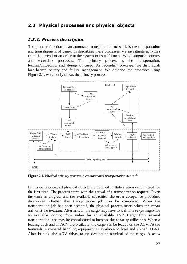
27

��' �6?�:��7��876?�:��>��

�� "��

The primary function of an automated transportation network is the transportationand transshipment of cargo. In describing these processes, we investigate activitiesfrom the arrival of an order in the system to its fulfillment. We distinguish primaryand secondary processes. The primary process is the transportation,loading/unloading, and storage of cargo. As secondary processes we distinguishload-bearer, battery and failure management. We describe the processes usingFigure 2.1, which only shows the primary process.

Loadtransported

to dock

AGVloaded

AGV sentto dock

AGV drives todestination

Empty AGVarrives atterminal

Cargotransported

to buffer

Cargo arrivesin terminal

Loaded AGVarrives atterminal

AGV sentto dock

AGVunloaded

Cargotransported

to buffer

AGV sent toparking place

Cargo leavesterminal


AGV in parking area

CARGO

AGV


Consolidation

Break upconsolidated

loads

Figure 2.1. Physical primary process in an automated transportation network

In this description, all physical objects are denoted in Italics when encountered forthe first time. The process starts with the arrival of a transportation request. Giventhe work in progress and the available capacities, the order acceptance proceduredetermines whether this transportation job can be completed. When thetransportation job has been accepted, the physical process starts when the cargoarrives at the terminal. After arrival, the cargo may have to wait in a cargo buffer foran available loading dock and/or for an available AGV. Cargo from severaltransportation jobs may be consolidated to increase the capacity utilization. When aloading dock and an AGV are available, the cargo can be loaded on the AGV. At theterminals, automated handling equipment is available to load and unload AGVs.After loading, the AGV drives to the destination terminal of the cargo. A track

28

system is required to enable vehicles to reach the destinations. Junctions, branches,two-way tracks and roundabouts may be included in this track system. A specialtype of track is the two-way track, which is a single track along which traffic in twodirections is possible (although not simultaneously). Hence, when the track isoccupied by vehicles travelling in the opposite direction vehicles have to wait,thereby causing additional delay. Once the AGV arrives at the destination terminal,it needs to unload at an unloading dock. When an unloading dock is available, theAGV drives to it, otherwise the AGV can be parked in a parking place or wait at theterminal entrance. When an unloading dock is assigned to the AGV, it drives to thatdock and the cargo is unloaded. Consolidated loads are broken up according to theoriginal transportation jobs. After spending some time in the terminal cargo buffer,the cargo eventually leaves the terminal. The empty AGV can be sent to a loadingdock, a parking place, another terminal or to a parking area. A loading and anunloading dock can be two different physical objects, but these two functions canalso be incorporated into one physical object.

Secondary processesSecondary, supporting processes may be associated with the logistics of sharedmovable resources, such as batteries and load-bearers. If the battery of an AGV isexplicitly modeled, it can follow a similar process to that of the cargo (notrepresented in Figure 2.1). In this case a battery is charged at a battery station andhas to wait in a battery buffer until it is needed by an AGV. When an AGV needs afully charged battery, it is sent to a battery station. The AGV has to be assigned to abattery dock where the battery can be changed. The battery is transported from thebattery buffer to the battery dock, where it is exchanged for the nearly empty batteryof the AGV. The nearly empty battery is sent to a charging station and whensufficiently recharged, is transported to the battery buffer and ready for reuse.Another option is to recharge the battery inside the AGV, in which case the AGV issent to a battery dock, where it is coupled to chargers. There the AGV has to waituntil the battery is sufficiently recharged.

To transport cargoes of different dimension load-bearers may be required. A load-bearer might also be required to secure the cargo. Empty load-bearers have to bemoved between the terminals to ensure that there are sufficient load-bearersavailable at every terminal to transport the transportation jobs present at thatterminal. When temporarily not needed, the load-bearer is stored in a load-bearerbuffer.

Another secondary process that interferes with the processes in Figure 2.1 is thefailure process. Equipment, such as AGVs and docks, can break down. BecauseAGVs move through the system and may block traffic in the case of failure, specialattention must be paid to AGV recovery. A failed AGV should be taken out of thesystem for repair. A special recovery vehicle must be available to tow the AGV tothe location at which it can be repaired. Note that it is not always necessary to

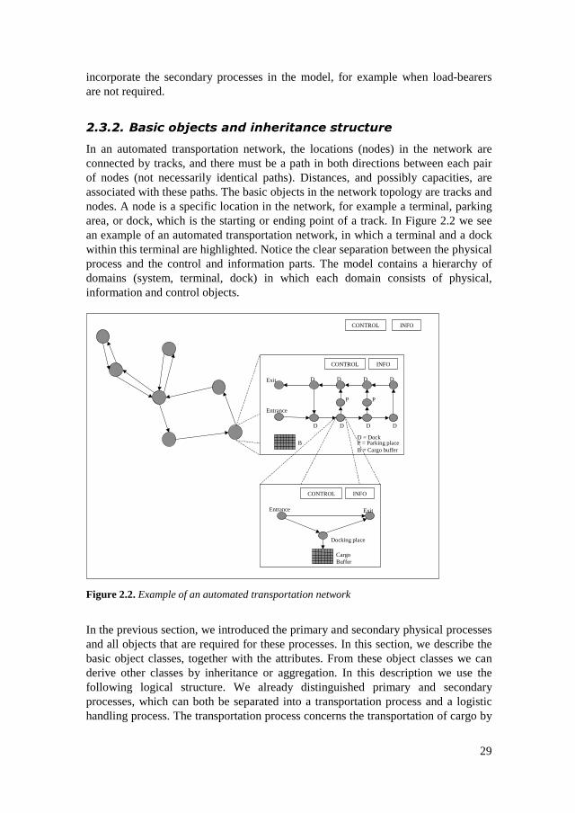
29

incorporate the secondary processes in the model, for example when load-bearersare not required.

�� $ ��

In an automated transportation network, the locations (nodes) in the network areconnected by tracks, and there must be a path in both directions between each pairof nodes (not necessarily identical paths). Distances, and possibly capacities, areassociated with these paths. The basic objects in the network topology are tracks andnodes. A node is a specific location in the network, for example a terminal, parkingarea, or dock, which is the starting or ending point of a track. In Figure 2.2 we seean example of an automated transportation network, in which a terminal and a dockwithin this terminal are highlighted. Notice the clear separation between the physicalprocess and the control and information parts. The model contains a hierarchy ofdomains (system, terminal, dock) in which each domain consists of physical,information and control objects.

CONTROL INFO

ExitEntrance

INFOCONTROL

CargoBuffer

Docking place

D

D

DD D

DD D

PP

Exit

Entrance

P = Parking placeB = Cargo buffer

D = Dock

INFOCONTROL

B

Figure 2.2. Example of an automated transportation network

In the previous section, we introduced the primary and secondary physical processesand all objects that are required for these processes. In this section, we describe thebasic object classes, together with the attributes. From these object classes we canderive other classes by inheritance or aggregation. In this description we use thefollowing logical structure. We already distinguished primary and secondaryprocesses, which can both be separated into a transportation process and a logistichandling process. The transportation process concerns the transportation of cargo by

30

the AGVs, whereas the logistic handling process deals with the loading/unloadingand storage of cargo, batteries and load-bearers. In these processes we distinguishthree elements: a flow unit, a handling unit and a storage unit. In this section theseunits (objects) will be defined for the different processes. First this will be done forbasic units, after which composite units will be considered. To avoid lengthyattribute lists, we note that as attributes, all objects have certain references to otherobjects and status indicators. There are references between objects to indicate whichobject is handled or stored by another object. For example, cargo contains areference to its position, whether this is a specific cargo buffer or an AGV. A cargobuffer has references to the cargo currently stored in the buffer. The status indicatorsare different for the three elements. The status of a handling unit is free/occupiedand up/down. A flow unit has a current location, and the status of a storage unit isits occupancy.

Primary transportation processFlow unit: vehicleWe need two different vehicles in the object-model: AGVs transport cargo andrecovery vehicles tow failed AGVs (see secondary transportation process). Theseobjects have a lot in common. Therefore, we introduce a basic object class vehicle,from which the other two object classes will be derived by inheritance (sub-class).As attributes the vehicle object has length, speed, maximum speed, driving direction(forward, backward), up/down and the destination. An additional attribute is theenergy consumption rate. The energy consumption depends on slopes, speed, weightand the acceleration and deceleration. The AGV object inherits the behavior andattributes of the vehicle object, but some additional functionality and attributes haveto be included. An AGV is used to transport cargo and therefore the AGV has acertain capacity for cargo. The attribute ‘status’ indicates whether the AGV isloaded or empty. Since we only consider unit-load AGVs, the capacity of the AGVis always equal to 1 (see Chapter 1, Section 1.2.3). For the transportation process,the AGV is a flow unit, but the AGV is also a handling unit for cargo and load-bearers.

Handling unit: trackThe AGVs are “handled” by the tracks. For example the tracks are tunnels in anunderground transportation system or roads. Vehicles cannot pass each other on atrack, but parallel tracks can be used for passing. We define a track as an object onwhich vehicles can drive. The track has a specific length, capacity, driving directionand speed limit. A track has only one predecessor and one successor. Several objectsof the track system share a common behavior and can be derived by inheritancefrom the basic track object: junctions, branches and two-way tracks. All derivedobjects share the functionality of the basic object class track, but with additionalfunctionality and/or attributes. A junction is a track with more than one predecessor,while a branch is a track with more than one successor. A two-way track is a trackthe driving direction of which can be changed; it can alternately serve traffic fromtwo directions. The two-way track has two predecessors and two successors, one for

31

each direction. An important attribute of the two-way track is the driving direction.The two-way track control object determines this driving direction (cf. Section 2.4).

Storage unit: parking placeVehicles that are temporarily not needed can be parked in a parking place. Theparking place is derived by inheritance from the track object, but has specific controlmethods and attributes to account for its storage function. A vehicle needspermission to enter a parking place and when a vehicle receives a job it will leavethe parking place and drive toward a dock or another terminal. A parking place canbe dedicated to loaded or empty vehicles, or alternatively to recovery vehicles.

Primary logistic handling process: cargo handlingFlow unit: cargoCargo is transported by AGVs and is related to a transportation job (see Section2.6). Cargo has a weight and volume. The corresponding transportation jobdetermines the origin and destination of the cargo, together with the release time anddue time.

Handling unit: loading/unloading dockCargo has to be loaded onto or unloaded from an AGV at a loading/unloading dock.Several docks were mentioned during the description of the physical process: aloading dock, an unloading dock and a battery dock. These objects have severalcharacteristics in common and therefore we define a basic dock object. We define adock as a location where a specific operation can be executed on an AGV. Anattribute of the dock is the time required for a dock operation. A dock has aloading/unloading facility, which can be used for loading, unloading or both. Anattribute of the dock is its functionality: loading, unloading or both. Other dockobjects can be derived, the functionality of which alternates between loading andunloading, with a set-up time in between.

Storage unit: cargo bufferCargo that cannot be loaded directly, because no AGV and/or dock is available, orcargo that has to wait to leave the terminal, e.g. on a plane, has to be stored. Wedefine a basic buffer object, which has a finite capacity for storing flow units, suchas cargo, batteries or load-bearers. A buffer is dedicated to a specific class ofmoveable objects. The cargo buffer can only store cargo.

Secondary transportation process: AGV failure management (optional)Flow unit: recovery vehicleA recovery vehicle is used to tow failed AGVs. The recovery vehicle is derived byinheritance from the basic vehicle object. To be able to reach failed AGVs therecovery vehicle should be able to drive in two directions (forward and backward).Unlike the AGV, the recovery vehicle cannot move cargo and load-bearers.However, it can act as a handler for AGVs.

32

Handling unit: trackThe recovery vehicles use the same infrastructure as the AGVs: the track system.We refer to the primary transportation process for more details on the track object.

Storage unit: parking placeA recovery vehicle that is temporarily not needed can be parked in a parking place.This is the same storage unit as the one used in the primary transportation process.

Secondary logistic handling process: load-bearer management (optional)Flow unit: load-bearerA load bearer can be used when cargoes of different dimensions have to betransported. A load-bearer might be required to facilitate the use of standard materialhandling equipment, such as the loading/unloading dock. AGVs can be used totransport the load-bearers

Handling unit: loading/unloading dockGiven the fact that a loading/unloading dock is designed to handle load-bearers,these load-bearers can be loaded and unloaded by the same dock.

Storage unit: load-bearer bufferWhen a load-bearer is temporarily not needed it is stored in a load-bearer buffer.

Secondary logistic handling process: battery management (optional)Flow unit: batteryA battery supplies a vehicle with energy. Attributes of the battery are its actual andmaximum charge. This information is important in determining whether an AGVcan still perform a given job or whether the battery should be changed or charged.

Handling unit: battery dock and charge stationThe battery of an AGV can be charged inside or outside the AGV. When the batteryis recharged inside the AGV, it must be possible to make the necessary connectionto recharge the battery at the dock. Otherwise the battery dock must be able tosupply a fully charged battery to replace the nearly empty battery. An additionalhandling unit is required if the battery is charged outside the AGV, so a location isneeded where the batteries can be recharged. We define a charge station object,which has a specific capacity. This capacity indicates the number of batteries thatcan be recharged at the same time.

Storage unit: battery bufferRecharged batteries, or batteries that have to wait for space in a charge station, canbe stored in a battery buffer. This object is derived from the basic buffer object,dedicated to the storage of batteries.

33

�� %�� #�&'� ��()� �� *

In the previous section we described the basic object classes and the object classesderived by inheritance. Compound objects, in which several objects from theprevious section are combined, can be defined. These compound object classes arederived from other objects based on aggregation relationships, using the concept ofmodularity (see Figure 2.5). Below we describe the compound object classes, whichcan be related to the transportation process, to the logistic handling process or toboth processes.

Transportation: roundaboutA roundabout is a combination of tracks, junctions and branches, and thereforecompletely based on aggregation relationships. The capacity of a roundabout islimited, being related to the capacity of the underlying track objects.

Transportation: track systemA track system is a combination of tracks and derived track objects: branches,junctions, two-way tracks, roundabouts and parking places. Together these objectsconstitute the infrastructure for the vehicles.

Transportation: parking areaNot all AGVs are continuously needed in the system, because transportation flowsmay fluctuate. For the AGVs that are not needed for a while, a parking area can beincluded in the model. Such a parking area consists of a track system with a numberof parking places, which determine the limited capacity of the parking area.

Logistic handling: dock stationA dock station consists of a dock, tracks and a buffer. There should be at least oneplace (a track) for an AGV and also a storage location for a flow unit (cargo, batteryor load-bearer). Extra places for AGVs or extra storage locations might be presentfor the pre-positioning of AGVs and flow units to reduce the time betweensubsequent dock operations, and to maximize dock utilization.

Transportation and logistic handling: terminalThe terminal object consists of a track system (tracks, branches and junctions) toensure that the AGVs can reach all destinations inside the terminal. Dock stationsare present for loading and unloading of AGVs, and there is a cargo buffer for cargostorage. Optional objects in a terminal are parking places and a load-bearer buffer.Parking places may be part of the track system inside the terminal to increase theflexibility of the terminal. A load-bearer buffer is necessary when the correspondingsecondary process is incorporated in the model.

Secondary logistic handing: battery stationWhen AGVs receive their energy from batteries, rather than from other sources ofelectricity (e.g. charge-rails), it is necessary to charge them in a battery station. Sucha battery station contains both a track system and battery dock stations. A battery

34

buffer and charge stations are required when the batteries are recharged outside theAGV. Parking places are optional.

SystemThe total system consists of a number of locations and a track system, whichconnects these locations (cf. Figure 2.2). Terminals must be present in the system. Aparking area and a two-way track are optional objects. When the secondaryprocesses are modeled additional objects have to be present.

�� +� ��

Now that all required objects have been defined, we can construct class diagrams. Inthese diagrams we show the relationships between the different objects. Wedistinguish three possible relationships. First the inheritance relationship, indicatingthat an object class (sub-class) is derived from another class (super-class). Thisrelationship is depicted as a directed arc, with the head pointing to the super-class.Second, an aggregation relationship, indicating that an object is part of anotherobject. This relationship is represented by a connection with a dot at the end. Thedot is connected with the sub-aggregate. Third, a using relationship, in which oneobject uses the services of another object. The using relationship is represented by aconnection with an open dot at the end, indicating the client.

Figure 2.3 shows the transportation process. The track system consists of severalobjects, some of them derived by inheritance from the super-class track, and othersbased on aggregation relationships. The vehicles use (or are handled by) the tracksystem to reach their destination, and can be stored in a parking place.

Track system

Track

Two-waytrack

Branch Junction

Roundabout Recoveryvehicle

AGV

Vehicle

Parkingplace

inheritance

aggregation

using

Figure 2.3. Class diagram of the objects that are part of the transportation process

Notice that the secondary process of AGV failure management is also included inFigure 2.3. The recovery vehicles use the same infrastructure as the AGVs. Thelogistic handling process is shown in Figure 2.4. These processes consist of ‘using’

35

relationships. The flow items (cargo, battery, load-bearer) are handled by (or use)the handling and storage objects.

Loading/unloadingdock

Load-bearerbuffer

Load-bearer BatteryCargo

Batterydock

Vehicle

Cargobuffer

Batterybuffer

Chargestation

Figure 2.4. Class diagram of the objects that are part of the logistic handling process

The using relations between cargo and load-bearer and between vehicle and batteryindicate the relationships between the primary and secondary processes in thelogistic handling. Cargo might need a load bearer for the handling at theloading/unloading dock. A vehicle might need a battery to provide its energy. In thiscase this secondary process, battery management, is included in the model.

In Figure 2.5 we see the network structure and the hierarchical decomposition. Wedistinguish three different levels for logistic control and transportation management:system level, terminal level (2) and sub-terminal level (3).

Batterystation

Terminal

Loading/unloading

dock

Batterydock

Tracksystem

System

Batterybuffer

Network structure

Parking area

Cargobuffer

Tracksystem

1

3

2

Chargestation

Load-bearerbuffer

Figure 2.5. Class diagram of the network structure and hierarchical decomposition

Notice that the track system appears at both lower levels (2 and 3). The track systemat the 2nd level connects the terminals, parking areas and battery stations, while theseobjects contain their own internal track system.

36

��* �� 9� 9��

It is not sufficient to model physical elements alone, since for an operational systema logistic planning and control structure is required. Control objects take care ofdecisions on the activities of physical objects within the area of their control.Furthermore, control objects use information available to them to ensure efficientuse of the physical objects and to achieve certain performance targets. Availableinformation includes the data stored in the control objects own accompanyinginformation object and data that can be accessed by an information request toanother information object. We return to this information issue in Section 2.6.

As explained in Chapter 1, we allow for hierarchical decomposition of the controlover several levels, for example over network and terminal levels. This allows for alocal control concept, with the possibility of central coordination and informationexchange between the controllers (managers). This means that the node managersare responsible for all control activities inside the nodes, but they can receiveperformance targets on their activities or even job definitions, such as empty vehiclejobs, from a higher level in the object hierarchy to ensure coordination between thenodes or levels. If local problems are solved locally and network problems centrally,we can construct a relatively simple and robust control structure without excessiveinformation exchange.

Local control does not necessarily mean significant loss of performance, providedthat appropriate information exchange between objects takes place. In the case oflocal control, the terminal manager bases its planning decisions and controlactivities on local terminal information only (embedded in the terminal informationobject). Insofar as other information is useful to optimize local decisions, thisinformation can be obtained by communication with other information objects. Weallow for local controllers that communicate with each other, either directly orindirectly via a common global controller. The local and global controllerscommunicate with each other in order to tune the effects of local decisions, and thusprevent negative effects of sub-optimization as much as possible. In Chapter 4 wewill analyze the effect of central versus local decision making on the logisticperformance. Now we consider the relation between the control objects and thephysical objects in more detail. Basically, each control object is uniquely associatedwith a physical object of a certain aggregation level. The control activities and theaggregation level (cf. Figure 2.5) are represented in Table 2.1, and are related to theclassification in primary/secondary processes and transportation/logistic handlingprocesses.

37

Table 2.1. Control activities and related objects

Primary process control Control activity LevelTransportation and logistics Local empty vehicle management 2

Vehicle scheduling 2

Transportation Global vehicle management 1Local vehicle control 2Two-way track control 2,3Routing control 2,3Traffic control 2,3Distance control 3

Logistics Order acceptance 1 (2)Consolidation control 2Order release 2Task allocation to docks 2Dock control 3

Secondary process controlTransportation and logistics Battery management 1,2

Load bearer control 1,2Failure management (AGVs, docks) 1,2,3

The control objects investigated in detail in the following chapters include vehiclemanagement, two-way track control, battery management and failure management.Although it is also interesting to study the other control objects, we chose to specifyonly one variant (see Section 2.5 for the corresponding definitions). In the next twosections we describe the function of the primary (Section 2.4.1) and secondaryprocess control objects (Section 2.4.2).

�� "� #��

Vehicle management can be considered at two hierarchical levels, namely atnetwork level (how to allocate empty vehicles amongst terminals and parking areas)and at terminal level (how to handle a vehicle in a terminal). At terminal level, it iseasier to react to unexpected events, such as the arrival of rush orders and the failureof docks or AGVs. All information required to make a good decision is available atthis level. At network level, we can focus on balancing vehicle flows, without takinginto account all detailed events at terminals. To this end, we distinguish betweenglobal vehicle management that covers the network level and local vehiclemanagement that covers the terminal level. From a practical point of view such anapproach is to be preferred, but it requires fine-tuning between the two hierarchicallevels.

38

Transportation and logistic handling controlLocal empty vehicle managementWhen an empty AGV becomes available, it is necessary to decide whether the AGVwill be used for an empty vehicle job (an empty trip) or for a transportation job. Anempty vehicle job is an assignment of global vehicle management to send an emptyvehicle to another terminal within a specified time window. A transportation job isan assignment to transport a load from origin to destination within a specified timewindow. If no jobs are present the AGV can be passed to local vehicle control. If theAGV can be used for a transportation job, the AGV is passed to vehicle scheduling.

Vehicle schedulingVehicle scheduling is the assignment of an AGV to a loading or unloading job. Anempty AGV can be assigned to a loading dock in combination with a transportationjob, while a loaded AGV can be assigned to an unloading dock to start an unloadingoperation. Here the transportation and logistic handling process come together. If nojob can be assigned to an AGV, the AGV receives a destination from local vehiclecontrol.

Transportation controlGlobal vehicle managementThe function of the global vehicle manager is to ensure that the AGVs are at theright network node at the right time. This is required to ensure that all transportationjobs are carried out. Global vehicle management is the topic of Chapter 4.

Local vehicle controlLocal vehicle control selects a destination for a vehicle that cannot be assigned to aspecific job, that is when there is no empty vehicle job or load job for an emptyAGV, or no unload job (no dock available) for a loaded AGV. A loaded AGV has tobe positioned somewhere in the terminal, e.g. a parking place, while an empty AGVcan also be sent to an empty dock or a parking area.

Two-way track controlThe function of two-way track control is to determine the time at which the drivingdirection of the two-way track should be switched. Two-way track control is part ofthe track system (level 2 and 3) and is considered in Chapter 5.

Routing controlGiven the location of a vehicle, and the destination of this vehicle, a travel routefrom the current location to the destination must be determined. The routing ofvehicles is a control object of the track system. At branches a vehicle must be sent inthe right direction (corresponding successor).

Traffic controlTraffic control is an object of the track system and has to prevent deadlocks andensure that traffic circulates freely. A deadlock is a situation in which vehicles are

39

blocked by other vehicles in such a way that the situation cannot be resolved.Furthermore, in order to prevent the average speed from being significantly reducedthe vehicles must not hinder each other too greatly.

Distance controlThe function of distance control is to prevent the collision of a vehicle with anotherobject. Therefore, distance control is incorporated in the vehicle object.

Logistic handling controlOrder acceptanceWhen a transportation request arrives in the system, order acceptance has to decidewhether the transportation job is accepted or declined. The order acceptanceprocedure may also be part of terminal control, but with communication between theterminals.

Consolidation controlThe function of consolidation control is to consolidate cargo into unit-loads. Such aunit-load will be translated to a transportation job for an AGV. Cargo that isconsolidated to one unit-load should have the same destination. Breaking up theseunit-loads at the destination terminal is also incorporated in this control object. Wedo not consider the case of several pick-up and delivery terminals. Consolidationtakes place at a terminal.

Order releaseBy order release we mean the assignment of transportation jobs to load docks in theterminal of origin (level 2). It is necessary to determine which order is sent to a dockand when an order is to be sent to a dock for loading.

Task allocation to docksDocks on a terminal are used for loading and unloading of AGVs. A dock canperform both loading and unloading operations at the same time. This has adisadvantage from a logistic point of view because the incoming and outgoing flowscannot be clearly separated. To separate these flows we can change the functionalityof the loading/unloading dock periodically, from loading to unloading and vice-versa. The control object under consideration determines the timing at which thefunctionality of each dock should be switched. Changing the functionality of a dockhas as an advantage over dedicated loading and unloading docks in that the dockcapacity can be fitted to the expected workload. A drawback is that setup times maybe involved.

Dock controlThe docks load and unload the vehicles or change (charge) the battery of an AGV.Dock control is responsible for the transfer of cargo (or battery) from the dock to theAGV and vice versa.

40

�� ,�� #��

Battery managementThe function of battery management is to ensure that batteries have sufficient chargeto perform the current job of the AGV they are provisioning with energy, and thatthe AGV does not stop somewhere in the system with an empty battery. Batterymanagement is required when AGVs have to change or charge their batteries at adock in a battery station. A decision should be made on the timing and location ofbattery change/recharge. Battery management is one of the topics in Chapter 6.

Load-bearer controlLoad-bearer control has to arrange that load-bearers are in the right place at the righttime. It must prevent situations arising in which transportation jobs cannot be loadedbecause there is no load-bearer available. In this thesis this aspect is not taken intoaccount; we assume that there are always sufficient load-bearers present whenneeded.

Failure managementThe resources are subject to failures, particularly AGVs and docks. Given a limitedfailure handling capacity, failure management focuses on the most efficient recoveryof equipment. Its purpose is to minimize downtime and to reduce the negativeeffects on system performance, for example by removing an AGV that is blockingtraffic as quickly as possible. The decisions involved are the assignment of recoverycapacity to failed equipment and, in the case of AGV failures, the reservation oftracks for the recovery vehicle to approach the AGV and the release of the tracks forregular traffic afterwards. Clearly, failure management requires coordinationbetween several control objects. Failure management is described in detail inChapter 6.

��) ��:<�� 6�� >��

In Section 2.4 we discussed the control structure and the functions of the controlobjects. Now we have to design the control objects. In Chapter 1 (Section 1.2.3) wedecided to design several options for vehicle management and two-way trackcontrol. These topics will be discussed in Chapters 4 and 5. The secondary processesof failure management and battery management will be discussed in Chapter 6. Herewe survey the control objects that are not discussed or varied during the analyses inthe next chapters. Different implementations of the control objects are possible,from heuristics to optimization procedures, as long as these are real-time. Wedescribe the control activities from a local control perspective. When it emerges thata local control concept cannot reach the performance targets, it is possible tointegrate several of the control activities. The integrated object should then complywith all interface requirements of the individual control objects. For example, globalvehicle management and order release could be integrated, such that the global

41

vehicle manager also determines the order release sequence in the terminals toensure that the planning of the global vehicle manager is followed as closely aspossible (see Chapter 4). We describe the basic behavior of the control objects. Thisbehavior can be overruled in the case of integrated planning, when several decisionsare taken simultaneously (coordinated).

Transportation and logistic handling controlLocal empty vehicle managementEvery time an AGV becomes idle (after unloading) or when an empty AGV arrives,the AGV can be assigned to a specific job. Depending on corresponding priorities,such as a latest departure time, the local empty vehicle manager can assign the AGVto an empty vehicle job or a transportation job. It may be possible to combine thejobs; a transportation job is selected which has the same destination as the emptyvehicle job. In this way, two jobs are fulfilled at once. When no empty vehicle jobsand transportation jobs are available, the AGV receives a destination from localvehicle control. If a transportation job is selected, the AGV is handed over to vehiclescheduling.

Vehicle schedulingA loaded AGV has to be assigned to an unloading dock. The nearest availableunloading dock for a loaded AGV is selected because in this way the AGV isunloaded as quickly as possible. When no unloading dock is available, a destinationwill be assigned to the AGV by local vehicle control.An empty AGV should be assigned to a load job. If multiple load jobs are available,the AGV is assigned to the dock with the highest priority order (see order release)that is released but not yet scheduled (no vehicle is assigned).Vehicle scheduling is also called when an unloading dock becomes available or anorder is released (new load job). Vehicle scheduling tries to select an AGV for theloading/unloading job. For both jobs the nearest AGV is selected; this matches withthe other control objects and ensures that dock utilization is maximized.

Transportation controlLocal vehicle controlAGVs that cannot be assigned to a specific job have to receive a destination. Aloaded AGV will be sent to the parking place closest to the first available unloadingdock. This maximizes dock utilization and minimizes the waiting times of theloaded AGVs. Information about start-times of the dock operations and the averageunloading time is required for this rule (cf. Section 2.6).An empty AGV can be positioned at an idle loading dock (no transportation jobpresent), or at a parking place. Again, the parking place closest to the first availableloading dock will be selected. If there are several idle loading docks, the AGV issent to the nearest loading dock. This pre-positioning minimizes waiting times whena transportation job arrives. If no new transportation jobs are expected in the nearfuture, the empty AGV might be sent to a parking area.

42

Routing controlRouting control has to assure that the vehicles arrive at their destination. Routingcan be done dynamically, in such a way that at every branch the currently fastestroute to the destination is determined. Such a routing strategy can be importantwhen there are a lot of alternative routes and the vehicles hinder each other on theroutes. We implement routing control according to a static routing algorithm. Onroutes between terminals for much of the time there are no real alternatives. Therouting of vehicles is implemented through a standard shortest path algorithm(Dijkstra, 1959). This shortest path algorithm is solved once for all origin-destination pairs. The results of these computations are stored in the layout. Allbranches have a destination list, indicating which direction should be followed,given the destination of a vehicle. Therefore, all vehicles travel along the shortestpath from origin to destination; no routing flexibility is incorporated.

Traffic controlTRACES (TRAffic Control Engineering System) is a traffic-control system whichcan handle high traffic densities and which was developed by Evers et al. (1999,2000) and modified by Verbraeck et al. (1999). TRACES fulfils the tasks ofmanaging the scarce infrastructure by providing routes to AGVs and bysafeguarding potentially unsafe parts of the infrastructure (e.g. because of collisionrisk). Analogous to the control systems at the network level, these tasks aredecentralized: the AGV executes its script that contains script statements, describingthe route to take and the locations along the route where a conflict might arise. TheAGV gets its script from the script dispatcher control object, which has a virtualmap of the terminal. When executing its script, the AGV requests access to conflictlocations, such as junctions or crossings, at local semaphores. If successful, theAGV receives a ticket, which it returns after leaving the conflict location. Thescripts, which can be assigned by the script dispatcher, are based on a wide range ofconditions, such as the traffic density in different areas, the destination of the AGV,information about failures, and the actual status of the AGVs battery. Furthermore,intelligence can be added to the scripts as well, so that the AGV can select the leastdense route dynamically. Notice that routing control is incorporated in this concept.We model traffic control rather simply. As long as there is capacity on a track avehicle can enter the track. On larger track configurations, such as roundabouts, welimit the number of vehicles: a semaphore is used to control the area. Thissemaphore is necessary to prevent deadlocks. The value of this semaphore isdetermined experimentally. Deadlocks also have to be prevented on terminals. Aterminal semaphore is also used to reduce the traffic on the terminal, therebyincreasing the average speed on the terminal by reducing the number of interactions.

Distance controlDistance control should be included to ensure that vehicles always remain at a safedistance from other vehicles. This minimum distance depends on the speed of thevehicle and the communication and reaction times. If a vehicle breaks down, theother vehicles should still be able to stop, without colliding. By using such distance

43

control, vehicles should continuously check the intermediate distance with respect toother vehicles. This introduces a lot of events. We implement a simplified distancecontrol, which is not implemented in the vehicle. It can be considered a separatecontrol object installed at the entrance of bottleneck infrastructure or the exit of acertain track object. When it appears that safety distances between AGVs haveserious impact on system performance, the model can check the intermediatedistances at certain locations, for example the exit of a terminal and the entrance of atwo-way track. If the intermediate distance is smaller than the required distance, thelast AGV will have to wait until the required distance is reached. We control theintermediate distance at the entrance of the two-way track. Assume that 60 AGVsare waiting in front of the two-way track and have to enter this two-way track. Whenan intermediate distance of 2 seconds is required between AGVs, given themaximum speed and maximum deceleration, it will take two extra minutes for allAGVs to enter the two-way track. Therefore, AGVs at the other end also have towait 2 more minutes before they can enter the two-way track. Neglecting this effectmight have a large impact on system performance. Intermediate distances could alsobe controlled at other locations in the network. We did not implement this becausethe AGVs in the simulation model seldom leave nodes less than several secondsapart.

Logistic handling controlOrder acceptanceIn our model we assume that all transportation jobs are accepted. We do not havesufficient information about the revenues of the different transportation jobs.Furthermore, we want to determine resource requirements for a future system. Thissystem should be able to handle the projected transportation demand. Wheninformation on actual revenues of transportation jobs is available one can estimatethe chance that a transportation job with higher revenues arrives in the near future(cf. Yield management, Smith et al., 1992).

Consolidation controlOn the terminal several rules can be used to consolidate cargo to unit-loads. Volumeand weight in particular are important for the physical possibility of consolidation.Furthermore, the destination and due times are important data used to determinewhether it is attractive to combine several cargo units. Here, we do not takeconsolidation into account, but rather we assume that all transportation jobs concernunit-loads.

Order releaseOrder release is the assignment of a load to a dock when a place at a dock is orbecomes available. At each dock station, one or more loads can be placed in a cargobuffer, waiting to be loaded. When a load enters a terminal of the OLS system, it isassigned to the loading dock with the shortest queue of unprocessed transportationjobs. If all cargo buffers of dock stations are occupied, the load waits in the terminalcargo buffer until a buffer position at a dock becomes available. At that time, the

44

transportation job with highest priority is released. Transportation jobs are releasedaccording to a priority rule based on minimum latest departure time. Recall that thelatest departure time is the time at which the cargo should leave the terminal oforigin to arrive with a high probability of arriving on time at its destination terminal.

Task allocation to docksTask allocation to docks is based on known and expected transportation jobs andrelated to the number of loading and unloading activities. Preferably the periodduring which the task allocation at a terminal is fixed (T) should be not too short andshould be attuned to the frequency at which the balance between load and unloadjobs changes.

Now, suppose that we have to decide on the number of dedicated loading andunloading docks for the next period with duration of T at time t0. The amount ofunload jobs is partly known from the number of loaded vehicles on the way toterminal i with expected arrival time before t0+T. Other information, for examplefrom demand forecasting, can be used to compute the total expected number ofunload jobs. Some of the load jobs in the next period are known, and information onadditional jobs can be demanded from demand forecasting. However, not all loadjobs have high priority, whereas unload jobs on transport to terminal i occupyAGVs, and should preferably be unloaded without delay. Therefore, we give ahigher priority to unload jobs than to load jobs. The procedure is as follows:1. Calculate the number of unloading docks required to process all (predicted)

unload jobs without much delay, given maximum dock utilization ρ. Themaximum utilization ρ is a control parameter that can be used to avoidexcessive waiting times at the docks.

2. Calculate the number of loading docks required for all (predicted) load jobs.3. If there are no excess docks, priority is given to unload jobs.4. If the total number of docks required for all jobs is less than the number of

docks available, allocate subsequently additional docks to the task for which theutilization is highest.

Using this rule, the maximum utilization for loading and unloading is minimizedheuristically. Because order arrivals are random, it can be expected that delay inorder processing will be reduced.

Dock controlWhen an empty AGV enters the dock station, the dock manager has to checkwhether the cargo is on the dock and the transfer can start. When cargo arrives at thedock, the dock manager also has to check whether an empty AGV is waiting to beloaded. The technical details for the transfer of the cargo, such as the informationexchange between AGV and dock, are not modeled. After unloading, the dockmanager will send the cargo to the terminal cargo buffer, and the AGV requests anew destination from the local vehicle manager.

45

Secondary process: Load-bearer controlLoad-bearers should be present when cargo has to be loaded. Therefore, relocationof load-bearers might be required to ensure that enough load-bearers are available atthe different terminals, especially if there are unbalanced transportation flows. Weassume that there are always load-bearers available, and we do not explicitly modelload-bearer control.

��0 ��=� :�� 9� 9��8:��=� :��>��

Information exchange between objects is required in a local control concept. First,we distinguish information that becomes available during the process, but cannot beinfluenced, such as transportation demand. Secondly, for the evaluation of thesystem, we need performance information as model output; this is only recorded andnot used by other processes. Thirdly, we distinguish information that can be used toimprove control decisions (see Figure 2.6). The purpose of the information structureis to ensure that the necessary information is at the right place at the right time, witha minimum of information exchange.

We distinguish two approaches to obtaining the required information from otherobjects: the pull approach and the push approach. When using the pull approach,information is requested from a specific object when it is needed. This approachprevents information exchange at moments when this information is not needed byother objects. It might not always be possible to use the pull approach. For example,when communication with AGVs is not possible at all times, the AGVs cannot beasked for the value of their attributes and the push approach should be used. In thepush approach an object communicates all its attribute changes to the objects thatrequire this information. The object that receives this information maintains theinformation in its local database. Information that requires a reaction or responseshould always be push, for example the completion of a job. A disadvantage of thisapproach might be the enormous amount of information exchange and high datastorage requirements. For example, each time an attribute of an AGV changes,communication will take place and this information has to be stored locally until it isneeded for a control decision.

Depending on the information that has to be exchanged, one can choose either thepull or push approach. In trying to minimize the information exchange in the system,we could use the following strategy. Information that is required very often, butwhich does not change frequently, can best be communicated via a push approach.Information that changes frequently, but is not required very often, might better becommunicated by using a pull approach. Between two information requests, thevalue of an attribute might change often, but the values in between two requests willnot be used. Information that changes infrequently and is also used infrequently, canbest be communicated by a pull approach. For cases of frequent change and frequent

46

use, both options can be considered and the amount of information exchange can bemeasured in a simulation study. Note that, in addition to information exchange, thetime available to make a decision is also relevant. If a decision has to be madealmost instantaneously, a pull concept could be impossible because of thecommunication time required.

��-�� .�� /��

Information objects gather information from a set of physical objects, such as allAGVs, and this information is made available to the corresponding control objects.Attributes can be seen as the information object at the lowest level. In case of a pushapproach, the information will be stored in the accompanying information object atthe same level. Now we will specify the most important communication lines (seeFigure 2.6) and the information that is exchanged on these lines. For the overview,control and information objects are only separated for the higher levels (network andterminal). The terminal control object is the aggregate of all control activities thattake place within the terminal. The same holds for the other control and informationobjects in Figure 2.6.

Orderacceptance

Terminalinfo

Systeminfo

Performance info

Battery

AGVDock

Parkinginfo

BufferParkingplace

Systemcontrol

Terminalcontrol

Trafficinfo

Parkingcontrol

Two-waytrack control

Parkingplace

Two-waytrack info

Demandforecasting

Forecasting traveland handling times

Figure 2.6. Information exchange between control and information objects

General control informationForecasting travel times and handling timesTravel times and handling times play an important role in some of the controlactivities (especially vehicle management and task allocation to docks). Fluctuationsin these times arise from fluctuations in workloads. Forecasts of travel timesbetween terminals (system level) and on a terminal can be made. Actual travel times

47

and handling times are gathered in the model. Based on actual realizations theexpected travel time and handling time can be estimated. The handling time is thetime from the arrival at a dock at the terminal of origin until the unloading isfinished at the destination terminal.

Note that the mean and standard deviations of the handling time (Hij) can beestimated using a standard exponential smoothing procedure (see e.g. Silver et al.,

1998). The mean E[Hij] is estimated by )(ˆ nijµ :

)()1()( ˆ)1(ˆˆ nij

nij

nij Hαµαµ −+= −

where )(ˆ n

ijH is the nth observation of the handling time for a transportation job from i

to j, )(ˆ nijµ is the estimate for E[Hij] after n observations and α is a smoothing factor

(e.g., α = 0.8). The standard deviation σ[Hij] is estimated by )(*25.1 nijMAD , where

)(nijMAD denotes the mean absolute deviation after n observations. This quantity is

also estimated by exponential smoothing:

)()()1()( ˆˆ*)1(* nij

nij

nij

nij HMADMAD −−+= − µαα

These expected travel times and handling times are used in the planning procedurefor the AGVs and in setting priorities for transportation jobs (cf. Chapter 4), but alsoto determine expected arrival times of AGVs at terminal entrances or two-waytracks. The latter information can be used to improve two-way track control (seeChapter 5).

From the expected travel times and handling times, the latest departure time for atransportation job is derived. The latest departure time is used as a priority rule forscheduling the transportation jobs (cf. Chapter 4). The latest departure time, tL,n, isset such that the due time for job n, tD,n, is met with high probability:

tL,n = tD,n – E[Hij]-kσ[Hij]

where k is a safety factor. The term kσ[Hij] allows for fluctuations in the handlingtime, caused by:• random loading and unloading times;• variation in travel times between locations in the network depending on local

origin/destination (dock in terminal, place in parking area);• unpredictable waiting time at the destination terminal, depending on workload.

We assume that Hij, which is the sum of the loading time, unloading time, traveltime and waiting time, is normally distributed. Hence, a reasonable value for k canbe found from the table for the standard normal distribution. For example, k=2.33

48

gives approximately a 99% probability that the transportation job will be handledbefore the due time, given that it leaves the terminal of origin at tL,n. By includingthe variation in the handling time, we set priority for an order that has higheruncertainty in handling time, for example because the distance is larger or becausethe destination terminal occasionally faces congestion.

Demand forecastingDemand forecasting predicts the transportation jobs for a specific future time period.Demand forecasting can take place at system or terminal level. Information aboutfuture orders is useful for task allocation to docks and empty vehicle management.Possibly, transportation jobs are known for a certain time horizon. The terminalmanagers might forecast transportation jobs for each destination, and a possiblepriority class within a given time horizon, which is longer than the horizon of knownjobs. Forecasts can be based on historical data using standard procedures (cf. Silveret al., 1998). We use the average transportation flows derived from historical data(see task allocation to docks).

CommunicationOrder acceptance to system info: transportation jobs (push)Key input to a model of a transportation network are transportation jobs. Atransportation job corresponds to transporting one unit-load from origin todestination with a release time (arrival time at the terminal of origin) and a due time(the time at which the cargo should be available for further transport). Once atransportation job is announced, the information is available in the systeminformation object.

System info to terminal info: transportation jobs (push)Transportation jobs should be announced to the terminal of origin of the job. Theterminal control objects can use this information, e.g. for task assignment to docksand order release. This information is needed frequently and does not change, so wechose a push approach.

Traffic info to system info: AGV location (pull)The traffic system contains sensors (induction loops), where all passages of AGVsare recorded. At the moment that an AGV passes such a sensor, the information isrecorded in the traffic information object. The sensors naturally have a pushapproach; otherwise several sensors have to be approached to locate an AGV. Uponrequest, traffic information can give the approximate location of an AGV to systeminformation (pull). This information can be used to determine the approximatelocation of an AGV and the expected arrival time of an AGV at its destination or atother places on its route.

Traffic info to two-way track info: expected arrival time of an AGV (pull)The traffic information object has information about the approximate locations ofthe AGVs. Once the destination of an AGV is known, the route is given (static

49

routing) and therefore also the two-way tracks on this route. The traffic informationobject can provide the two-way track control object with information about theexpected arrival times of AGVs at the entrance of the two-way track. Either a pushor pull approach can be used in this respect, depending on the frequency with whichthis information is used. Considering the decision frequency and the number ofinformation updates, we chose to use a pull approach in our simulation model.

Track system to system and terminal info: distances (pull)For several control activities at system and terminal levels, distances betweenlocations are required, e.g. to find the nearest terminal or dock. This information canbe obtained from the track system. Since this information does not change, thesystem information object requests this information from the track system onlyonce. From the moment that the distance matrix is known, no furthercommunication is required. The same holds for the terminal information object, butonly distances on the terminal are of interest. Another option is to use travel timesinstead of distances. Travel times can change over time, but can be requested fromtraffic information (pull).

Dock to terminal control: status and functionality (push)Terminal control objects need to know the status and functionality of the docks forseveral control activities, and also the starting time of the last dock operation and theaverage dock operation time. When this information is needed, they can obtain itfrom the dock objects. Either a push or a pull approach can be used; we chose a pushapproach. When the status of the dock changes, for example the dock becomes idle,terminal control is notified and can directly take action.

AGV to terminal control: status (pull), presence (push)The terminal control objects need information about the status of the AGVs on theterminal. This information is requested from the AGVs. When an AGV enters aterminal, the responsibility for this AGV changes from the global vehicle managerto the local vehicle manager. The terminal information object will maintain a list ofthe AGVs that are within the terminal domain.

AGV to system info: trip finished, status, destination (push)After finishing a particular trip (empty trip or a transportation job), an AGVcommunicates with system information. Realizations of travel times and handlingtimes are recorded for all origin-destination pairs. The handling time is the timefrom the start of loading the vehicle until the unloading is finished. The AGV alsocommunicates the battery charge that was required for a particular trip, usinginformation from the battery. The required battery charge for the different routes isimportant information for the secondary process of battery management.Control objects at system level, especially the global vehicle manager, needinformation about the status and destination of the AGVs. Because this informationis needed frequently, we chose a push strategy. The system information objectrecords and updates the information for all AGVs in the system.

50

Parking place to terminal and parking control: status, functionality (pull)The terminal and parking control objects might need information about the status,i.e. the number of available places, and the functionality, loaded or empty, of theparking places. This information is requested whenever necessary. Because thisinformation is not needed very frequently, and also the information does not changefrequently, we chose a pull approach.

System control to terminal and parking info: empty car jobs (push)When there is central coordination the global vehicle manager (part of systemcontrol) can send (push) empty vehicle jobs to the terminal and parking informationobject. Terminal control and parking control will take this information into accountin local vehicle management.

All information objects report to performance measurement: information forevaluation (push and pull)For all objects in the model, performance information can be recorded, for examplethe utilization of docks and AGVs or the throughput time of transportation jobs.These figures might be requested, for example every half-hour (pull), or can besubmitted after finishing a specific event, such as the fulfillment of a transportationjob (push). These figures can be aggregated over all objects in a certain class(AGVs), or for a certain object (terminal).

��-�� "��

The model should provide performance information that can be used to evaluateseveral alternatives with respect to system layout and control methods. A lot ofinformation can be extracted from the model. Examples of performance informationare shown in Table 2.2.

Table 2.2. Performance information

Objects Performance informationSystem number of orders on time, throughput time distribution

failure registration (docks and AGVs)Terminal average dock utilizationParking area occupationBattery station number of battery changes, average lost chargeTwo-way track average waiting times, convoy lengthsDock capacity utilization, failuresBuffer capacity utilization, maximum occupationVehicle driven distance (loaded and empty)Cargo on-time, throughput time

51

At system level, aggregated figures are available on the transportation jobs. Aftercompletion of a transportation job, we record whether the job was late, if late howlate it was and the throughput time, i.e. the time the job was completed minus therelease time. From these figures, the number of late orders and the throughput timedistribution can be determined per origin-destination pair, and can be aggregated forthe total system. To evaluate system performance, the most important figure from acustomer’s point of view is the service level. This level indicates the percentage oftransportation jobs that is delivered on time at its destination. From the point of viewof cost, minimizing the empty kilometers might be attractive. Other importantinformation relates to the utilization of the resources. Low utilization throughout theentire day may indicate that the number of docks or AGVs can be reduced. On theother hand, high utilization rates may indicate a shortage of resources. If failures areincluded in the model, these are recorded at system level. The number of failures,the location of the failures and the duration of the failure are recorded. Dependingon the objectives of the research, one or more of these performance measures can beused.

��2 �9==��?

In this chapter we described an object structure for automated transportationnetworks, in which we distinguished physical, control and information objects. Theprocesses in such a transportation network were divided into primary and secondaryprocesses, and subdivided into transportation and logistic handling processes. Forthe different processes we distinguished flow, handling and storage units. Based onthis classification we designed an object model for automated transportationnetworks. We described the function of the physical, information and control objectsand the relations between these objects. Furthermore, we designed the controlobjects that are not the subject of further research in this thesis, and describedperformance measures that can be used in the evaluation of several alternatives withrespect to system layout and control methods.

53

�6�7 ��

'

��8��:7 :��( 6��:=9� :��

'�� 89� :��

In June 1994, the first discussions started about the possibility of using undergroundfreight transportation between Amsterdam Airport Schiphol and the flower auctionmarket at Aalsmeer. In this chapter we describe the OLS-project, which is used as acase study in this thesis. Our aim is to discuss the position of our mainly operationsresearch and simulation based research within the project. The main goal of thesimulation group within the OLS-project was to develop and evaluate logisticcontrol rules and to determine the logistic performance of the system in relation tolayouts and capacity. We first describe the project history in Section 3.2. Next, theactivities of the transportation and control technology group within the OLS-project,as part of the pre-design phase, are described in Section 3.3. The results of thisresearch, for example terminal, dock, AGV and control system design, constituteinput for our models. In Section 3.4 we describe the relevant estimates with respectto transportation flows. As one of the project goals is system dimensioning, inSection 3.5 we show to what extent analytical models can be used for this purpose.We develop a model that provides a rough estimate of the resource requirements andapply it to one of the proposed system layouts. As we will see, analytical models areonly partially useful for the estimation of resource requirements, and therefore wealso use simulation to determine more accurate resource requirements. Simulation isapplied to all the system layouts under consideration. In Section 3.6 we summarizeour contribution to the overall project and its relation to contributions from other

54

groups. Furthermore, we summarize the figures that will be used as input for thesimulation model in subsequent chapters.

'�� >�� 9� 9��

Three phases of the project have been finished since the start of the project: afeasibility study, a definition study and the pre-design phase. Our research was partof the pre-design phase. In this section we describe some results and conclusionsfrom these three phases.

�� 0� ��#��#

In 1995, the managers of Amsterdam Airport Schiphol and the flower auctionmarket at Aalsmeer initiated a feasibility study to investigate the possibility of usingunderground freight transportation. The Ministry of Transport, Public Works andWater Management, and the Holland International Distribution Council (HIDC)supported this initiative. A feasibility study (Van de Geijn and Katgerman, 1996)was designed to determine whether an underground logistic system betweenSchiphol Airport, the flower auction market, and a rail terminal could be justified onspatial, logistical, technical, organizational and economic grounds. The undergroundlogistic system was intended to transport time-critical products, such as flowers,dairy produce, newspapers and spare-parts. Speed, reliability and timeliness are veryimportant to such a system. The conclusions of the feasibility study were positive,but further research was required to determine the system layout, the diameter ofunderground tubes, the operating costs and the preconditions to be fulfilled in orderto generate an OLS associated, high-quality rail product, which does not yet exist.

�� #

Following on the feasibility study, a definition study was performed on the initiativeof Amsterdam Airport Schiphol, the flower auction market at Aalsmeer, NS Cargo,Railned, the Ministry of Transport, Public Works and Water Management, theHolland International Distribution Council, the Air Transport AssociationNetherlands (ATAN) and the Center for Transportation Technology (CTT). Themain conclusions of this definition study were (CTT, 1997):• The OLS contributes to the accessibility of Amsterdam Airport Schiphol and

the flower auction market at Aalsmeer.• The OLS relieves the roads in the neighborhood of Schiphol and Aalsmeer, and

as a result reduces the burden on the environment.• For Schiphol and Aalsmeer, the OLS is the missing link with rail transportation.• The transition from road transportation to the OLS and rail transportation is

feasible on economic grounds, given the forecasted growth in transportationflows.

55

• More research is required to corroborate the choice between a tube diameter of3.5 or 5 meter.

• More research is needed to compare various system designs.• More research is required on the technical and logistical control of AGVs, the

design of loading/unloading equipment, and on drilling in soft soil.

�� "�1��

The results of the definition study were sufficiently positive for the pre-design of thesystem to be started. The goal of this pre-design phase was to refine the results ofthe definition study and to prepare plans for implementation. Some objectives of thisphase were (Van der Heijden et al., 2000):• to obtain adequate information for a go/no-go decision for the next phase, in

which the first part of the system will be constructed.• to deliver an optimized system design to the future owner of the infrastructure.• to deliver tested AGVs and loading/unloading technology to the system

operating company.• to design new control systems and hand these over to the operating company.• to test the prototype AGVs and loading/unloading docks, with their control

systems, at a test site.

Several research disciplines cooperated intensively to perform an integralassessment of this new transportation system, to optimize the system design, and toexplore its technological and economical viability. Among these research disciplinesare underground construction technology, AGV technology, automated docking andwarehousing technology, information and communication technology, controltechnology, logistics, simulation, and economics. An important aspect was tocontinuously involve a user-group in the definition of the research questions and theevaluation of the research results. In the pre-design phase, more than a hundredresearchers and developers at universities and research institutes, as well ascustomers and business partners were directly involved.

Three different project groups were installed. One project group focused on themanagement and exploitation of the OLS, another project group on undergroundconstruction, and still another group on the transportation and control system of theOLS. In the next section, we describe the activities of the project group ontransportation and control technology. For the results of the other two project groupsrefer to the reports from Schiphol Project Consult (2000) and Centrum OndergrondsBouwen1 (2000).

During the pre-design phase, several assumptions and specifications changed owingto additional insight obtained from the research. Examples of changes are the systemdesign, transportation flows, and AGV specifications such as speed and length, and

1 This is the Dutch name for “Center for underground construction”

56

docking times. Where relevant, we indicate which specific assumptions were usedfor which part of our research.

At present (March 2001), some details relating to questions that arose in the pre-design phase remain to be filled in. The AGVs and docks are still being tested at theTest Site to decide about a final AGV design. Furthermore, the internal processes atSchiphol Airport are being investigated to connect these processes to the OLS in thebest possible way, thereby considerably reducing the internal transportation atSchiphol Airport. Simulation studies still play an important role in this part of theproject. By the end of 2001 a decision should have been made about theimplementation of the OLS.

'�' �9�/7��>�� 7�� :��8�� 6��<?

In this section, we describe some aspects of the research done within thetransportation and control technology group. The activities regarding the design oflogistic planning and control rules and the network simulation were concentratedwithin this group. Here we give a brief summary of the main activities. In thesubsequent sections we distinguish system design, functional requirements, vehicles,terminal and dock design, operating and information system, simulation and theConnekt Test Site. For more details and results refer to Rijsenbrij et al. (2000).

�� ,#��

The OLS-system consists of three main locations: a Rail Terminal near Hoofddorpor the Zwanenburg runway (RTH or RTZ, respectively), the flower auction marketat Aalsmeer (VBA = “Verenigde Bloemenveiling Aalsmeer") and AmsterdamAirport Schiphol (AAS). One of the layouts that resulted from the definition study,and that was used for further research within the simulation group, is the Stommeerlayout (see Figure 3.1). RTH, consisting of one terminal, is located in the west,VBA, consisting of two terminals, in the southeast, and AAS, consisting of fiveterminals, in the north. The required number of terminals at each location, based oncosts and expected transportation flows (CTT, 1997) was determined in thedefinition study. AGVs that are not needed for a while, or for which there is nospace at the terminals, are dispatched to a parking area that is located just south ofSchiphol Airport, close to the central intersection. This central parking area is notshown on the map.

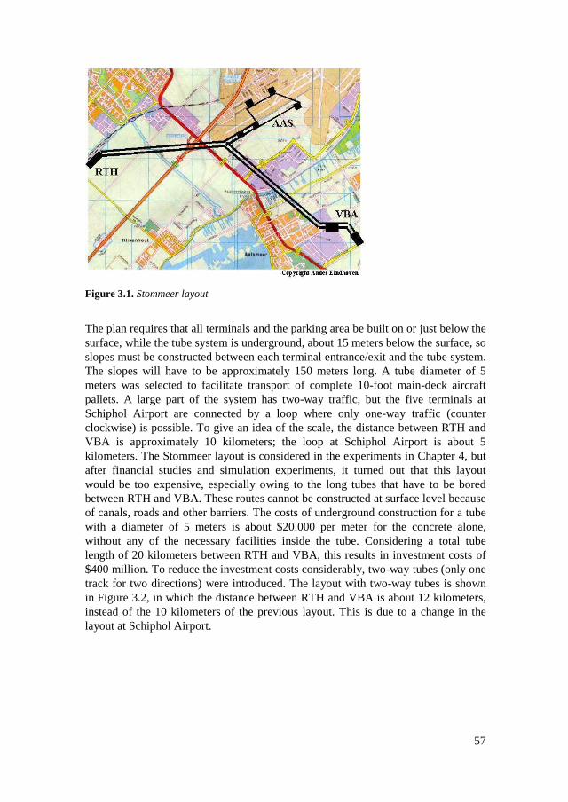
57

Figure 3.1. Stommeer layout

The plan requires that all terminals and the parking area be built on or just below thesurface, while the tube system is underground, about 15 meters below the surface, soslopes must be constructed between each terminal entrance/exit and the tube system.The slopes will have to be approximately 150 meters long. A tube diameter of 5meters was selected to facilitate transport of complete 10-foot main-deck aircraftpallets. A large part of the system has two-way traffic, but the five terminals atSchiphol Airport are connected by a loop where only one-way traffic (counterclockwise) is possible. To give an idea of the scale, the distance between RTH andVBA is approximately 10 kilometers; the loop at Schiphol Airport is about 5kilometers. The Stommeer layout is considered in the experiments in Chapter 4, butafter financial studies and simulation experiments, it turned out that this layoutwould be too expensive, especially owing to the long tubes that have to be boredbetween RTH and VBA. These routes cannot be constructed at surface level becauseof canals, roads and other barriers. The costs of underground construction for a tubewith a diameter of 5 meters is about $20.000 per meter for the concrete alone,without any of the necessary facilities inside the tube. Considering a total tubelength of 20 kilometers between RTH and VBA, this results in investment costs of$400 million. To reduce the investment costs considerably, two-way tubes (only onetrack for two directions) were introduced. The layout with two-way tubes is shownin Figure 3.2, in which the distance between RTH and VBA is about 12 kilometers,instead of the 10 kilometers of the previous layout. This is due to a change in thelayout at Schiphol Airport.

58

Figure 3.2. OLS layout with two-way tubes

Three two-way tubes are present in the layout, one between RTH and AAS (length2200 meter), one between AAS and VBA (2700m) and one at Schiphol Airport(750m). Further investment reductions were obtained by reducing the number ofterminals from 5 to 3 at AAS, and from 2 to 1 at VBA. The parking area (not on themap) is located at Schiphol Airport, near the left terminal (AAS1). The layout withtwo-way tubes is used in the experiments described in Chapter 6.

The reason for designing yet another layout was the request of Schiphol Airport toadjust the design, such that the system can also be used for internal transportation atSchiphol Airport (see Figure 3.3). The business parties at Schiphol want to reducethe number of freight trips on the airport; at present most trips at Schiphol carry lessthan a truckload. At Schiphol Airport 1st and 2nd line terminals are distinguished.The 1st line terminals are located at the loading and unloading platforms of aircraft.Terminals 5, 6, 7, 12, 14, 15 and 18 are 1st line terminals, the remaining ones are 2nd

line terminals. At present, trucks deliver to 1st line and 2nd line terminals, and thesize of their deliveries varies from 1 box to a full truckload. Once the OLS isoperational, trucks should deliver and pick-up cargo only at the 2nd line terminals. Inthe future, the OLS will take care of the transportation between 2nd line and 1st lineterminals. Possibly, some of the small 2nd line cargo handling companies will nothave their own connection to the OLS. For these companies, a cargo consolidationcenter can be constructed, where they can deliver and pick up their loads. This cargoconsolidation center will have its own OLS terminal. In this way, the truckmovements around Schiphol Airport can be reduced. Note that freight from severaldeliveries, but with the same origin and destination terminals within the OLSsystem, can be consolidated to form one transportation unit, thereby reducing thenumber of trips.

59

Figure 3.3. OLS with internal transportation system at Schiphol Airport

The number of terminals at Schiphol increases significantly in comparison with theprevious layout, from 3 to 18, but the size of the terminals decreases. The AASterminals are located on three loops at Schiphol Airport, with one isolated terminal.Terminal investment costs increase, but the costs of the tube network are decreasedby moving the rail terminal from Hoofddorp to Schiphol Airport. The two-way tubebetween the rail terminal and Schiphol Airport is removed, while the two-way tubebetween VBA and AAS remains. Notice that the distance between RTZ (renamedfrom RTH because of the location change) and VBA is almost halved, from morethan 10 to about 5 kilometers. The loops at Schiphol Airport are between 2 and 3kilometers long. The parking area is not represented in the figure, but is located onthe right loop at Schiphol (East). This layout is used in Chapters 5 and 6.

�� 0��

It is important for a successful implementation of the OLS that the system complieswith the expectations and demands of its users. The demands should be clear beforethe system is designed. These demands are related to (Rijsenbrij et al., 2000):• Transportation conditions: in particular temperature and humidity.• Reliability: with regard to throughput time requirements and service levels.• Availability: failures should have limited impact.• Accessibility: all users should be able to deliver their goods to the system.• Spatial planning: existing infrastructure should be taken into account.• The environment: the negative environmental effects should be limited.Simulation studies are playing an important role in assessing both the reliability andthe availability.

60

The OLS has to transport several cargo types: main-deck aircraft pallets, Euro-pallets, industry pallets, Danish carts and flower auction market carts. All thesecargo types have different weights and dimensions. We define a transportation unit(TU) as an amount of cargo, which is handled by the OLS as 1 unit. The loadingcapacity of an AGV can be expressed in TU. In the OLS-case a TU has the samedimensions as a 10 foot main-deck aircraft pallet: LxWxH=3.18x2.44x3.00 meter(Rijsenbrij et al., 2000). Given these dimensions, a TU can consist of:• 1 main-deck aircraft pallet• 6 industry pallets• 6 Euro pallets• 8 Danish carts• 4 flower auction market carts

The maximum weight of a TU is 3500 kilo. Special load-bearers could be requiredto make possible the standardization of the handling of these different cargo types,for example for loading and unloading of AGVs and to secure the cargo.

�� 2��

Automated Guided Vehicles (AGV) transport the cargo between the terminals of theOLS. Three prototypes were designed and built, one of which is shown in Figure3.4. The prototypes are based on different characteristics, but with some generalspecifications, which are used in the simulations (Rijsenbrij et al., 2000):• Normal speed: 6 m/s• Maximum speed on terminal: 2 m/s• Speed on slopes up: 3 m/s• Speed on slopes down: 6 m/s• Capacity of an AGV: 1 TU• Maximum weight of one TU: 3500 kilogram• Maximum acceleration/deceleration in a normal situation: 1 m/s2

• Maximum acceleration/deceleration in case of an emergency stop: 2 m/s2

• AGVs drive on rubber wheels in the terminals• AGVs are free-ranging in the terminals• AGVs are driven by an electric motor• At the terminals electricity is supplied by batteries

The three prototypes are used to test differences between two and four wheelsteering, rubber wheels and steel wheels on rails, rail guidance, electrical guidanceusing transponders or a magnetic grid, and self-guidance of the vehicles. For moreinformation on these vehicle designs refer to Rijsenbrij et al. (2000). A specialrecovery vehicle will be present to tow failed AGVs. This recovery vehicle has notyet been designed. The AGVs are controlled according to a local control principle.All AGVs control their own speed and distance with respect to other AGVs orobstacles (Verbraeck et al., 1998a).

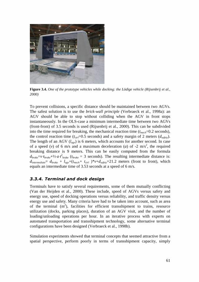
61

Figure 3.4. One of the prototype vehicles while docking: the Lödige vehicle (Rijsenbrij et al.,2000)

To prevent collisions, a specific distance should be maintained between two AGVs.The safest solution is to use the brick-wall principle (Verbraeck et al., 1998a): anAGV should be able to stop without colliding when the AGV in front stopsinstantaneously. In the OLS-case a minimum intermediate time between two AGVs(front-front) of 3.5 seconds is used (Rijsenbrij et al., 2000). This can be subdividedinto the time required for breaking, the mechanical reaction time (tmech=0.2 seconds),the control reaction time (tctrl=0.5 seconds) and a safety margin of 2 meters (dsafety).The length of an AGV (lagv) is 6 meters, which accounts for another second. In caseof a speed (v) of 6 m/s and a maximum deceleration (a) of -2 m/s2, the requiredbreaking distance is 9 meters. This can be easily computed from the formuladbrake=v⋅tbrake+½⋅a⋅t2

brake (tbrake = 3 seconds). The resulting intermediate distance is:dintermediate= dbrake + lagv+(tmech+ tctrl )*v+dsafety=21.2 meters (front to front), whichequals an intermediate time of 3.53 seconds at a speed of 6 m/s.

�� 3�� 4��

Terminals have to satisfy several requirements, some of them mutually conflicting(Van der Heijden et al., 2000). These include, speed of AGVs versus safety andenergy use, speed of docking operations versus reliability, and traffic density versusenergy use and safety. Many criteria have had to be taken into account, such as areaof the terminal (m2), facilities for efficient transshipment to trains, resourceutilization (docks, parking places), duration of an AGV visit, and the number ofloading/unloading operations per hour. In an iterative process with experts onautomated transportation and transshipment technology, some alternative terminalconfigurations have been designed (Verbraeck et al., 1998b).

Simulation experiments showed that terminal concepts that seemed attractive from aspatial perspective, perform poorly in terms of transshipment capacity, simply

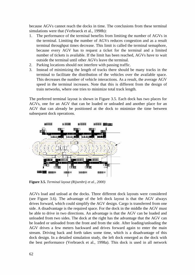
62

because AGVs cannot reach the docks in time. The conclusions from these terminalsimulations were that (Verbraeck et al., 1998b):1. The performance of the terminal benefits from limiting the number of AGVs in

the terminal. Limiting the number of AGVs reduces congestion and as a resultterminal throughput times decrease. This limit is called the terminal semaphore,because every AGV has to request a ticket for the terminal and a limitednumber of tickets is available. If the limit has been reached, AGVs have to waitoutside the terminal until other AGVs leave the terminal.

2. Parking locations should not interfere with passing traffic.3. Instead of minimizing the length of tracks there should be many tracks in the

terminal to facilitate the distribution of the vehicles over the available space.This decreases the number of vehicle interactions. As a result, the average AGVspeed in the terminal increases. Note that this is different from the design oftrain networks, where one tries to minimize total track length.

The preferred terminal layout is shown in Figure 3.5. Each dock has two places forAGVs, one for an AGV that can be loaded or unloaded and another place for anAGV that can already be positioned at the dock to minimize the time betweensubsequent dock operations.

Figure 3.5. Terminal layout (Rijsenbrij et al., 2000)

AGVs load and unload at the docks. Three different dock layouts were considered(see Figure 3.6). The advantage of the left dock layout is that the AGV alwaysdrives forward, which could simplify the AGV design. Cargo is transferred from oneside. A disadvantage is the required space. For the dock in the middle the AGV mustbe able to drive in two directions. An advantage is that the AGV can be loaded andunloaded from two sides. The dock at the right has the advantage that the AGV canbe loaded or unloaded from the front and from the side. After loading/unloading theAGV drives a few meters backward and drives forward again to enter the mainstream. Driving back and forth takes some time, which is a disadvantage of thisdock design. In a detailed simulation study, the left dock emerged as the dock withthe best performance (Verbraeck et al., 1998a). This dock is used in all network

63

simulations. In the definition phase, the loading/unloading time was assumed to be 2minutes, while this time was reduced to 1 minute during the pre-design phase. In thesimulations, we assume that the loading and unloading times are gamma distributed,with an average of 2 minutes and a standard deviation of 15 seconds (later decreasedto 1 minute and 6 seconds, respectively). The standard deviation is introducedbecause fluctuations in loading/unloading times may arise from cargoes of differenttype, size and/or weight.

Figure 3.6. Three different dock layouts (Rijsenbrij et al., 2000)

For the loading/unloading operation, a choice had to be made between rolling andlifting. An advantage of rolling conveyor technology is that it is proven technology,and no lifting device is required. Lifting requires expensive construction and isriskier in relation to possible load/vehicle damage in case of failures. An advantageof lifting technology is that no roller conveyor is required within the AGV. The finalchoice with respect to rolling or lifting has not been made yet.

At the terminal entrance there are two line-up tracks, one for loaded and one forempty vehicles (not shown in Figure 3.5). Queuing in front of the terminal entrancemay occur if an arriving vehicle cannot be assigned to a free destination in theterminal (dock, parking place), or if the maximum number of vehicles on theterminal has been reached (terminal semaphore). These line-up tracks operateaccording to the First-In, First-Out (FIFO) principle. Separate queues for loaded andempty vehicles offer flexibility to set priorities for either job type. Queuing mayhave an impact on the logistic performance, because loaded vehicles cannotovertake in the queue, whereas, given the different job priorities, this may bedesirable. Loaded and empty AGVs are parked in separate parking places, to ensurethat empty AGVs do not block loaded AGVs.

At Schiphol Airport space is limited and very expensive. Therefore, small terminalswere designed with only 1 or 2 docks, no parking places and no line-up track at theentrance. A drawback is that AGVs that wait at the entrance of a terminal block allother traffic, because all AGVs drive through the terminal. There are only twowaiting places next to the main track (see Figure 3.7), one at the dock and one placebehind the AGV at the dock. The space at the right side of the dock is required foracceleration.

64

Figure 3.7. Small terminal at Schiphol Airport (Rijsenbrij et al., 2000)

The rail terminal at Hoofddorp is shown in Figure 3.5, but the design of the railterminal near the Zwanenburg runway had to be different. The trains will bestationed in the middle of this terminal, while the docks are at the outside, with 3places for AGVs at each dock. A bridge or tunnel is required for vehicles to drive tothe other side of the terminal. Because the trains are in the middle of the terminal,there is no space for parking places or shortcuts. The terminal is very long and onetrip around the terminal is about 1 kilometer. To reduce the impact of these longdistances, the speed of vehicles on this terminal is increased to 4 m/s.

In all the system designs presented (see Section 3.3.1) there is 1 central parking areain the system. This parking area is used for AGVs that are not needed for a while,for example during the night. The parking area contains several parking lanes inwhich AGVs line-up. The capacity of the parking area should be sufficient toaccommodate all AGVs. Maintenance facilities can also be located at or near theparking area.

��5� %�� #��

Another important feature of the OLS-system is the operating and informationsystem. The most important tasks of such a system are (Rijsenbrij et al., 2000):• Order acceptance and order processing.• The planning of transportation jobs, such that the available resources are

efficiently used.• Operating the resources to ensure that these resources act at the right time at the

right place.• Supply of information on the actual state of the system, the history, the

performance characteristics and other relevant information.

Some of the planning and control rules needed for the operating and informationsystem are considered in this thesis, especially the higher levels concerned withtransportation planning in the system as a whole. These rules were evaluated byusing a simulation model, which is described in more detail in the next section. Formore information on the lower levels of, for example, AGV and dock control, referto Rijsenbrij et al. (2000).

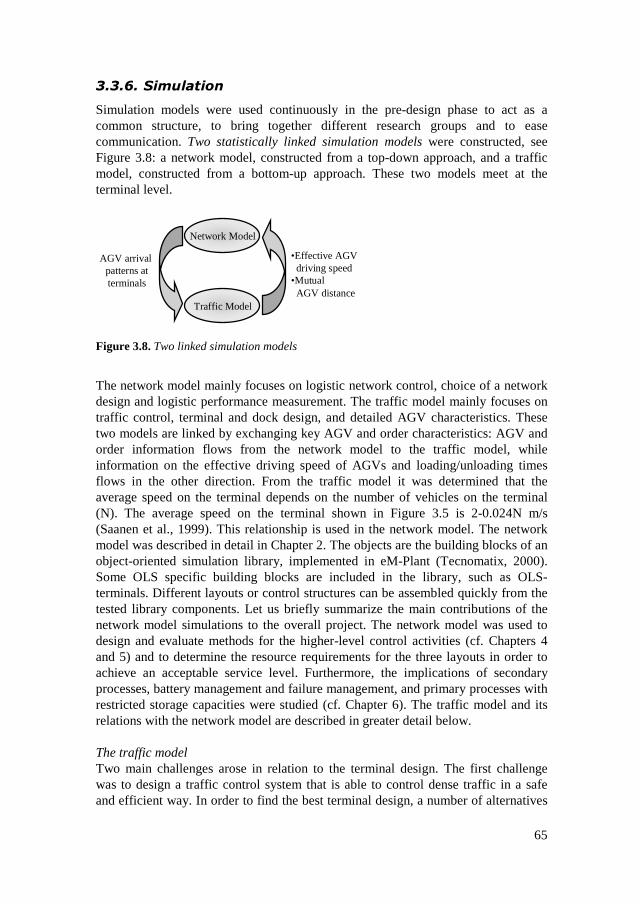
65

��-� ,��

Simulation models were used continuously in the pre-design phase to act as acommon structure, to bring together different research groups and to easecommunication. Two statistically linked simulation models were constructed, seeFigure 3.8: a network model, constructed from a top-down approach, and a trafficmodel, constructed from a bottom-up approach. These two models meet at theterminal level.

Network Model

Traffic Model

•Effective AGV driving speed•Mutual AGV distance

AGV arrival patterns atterminals

Figure 3.8. Two linked simulation models

The network model mainly focuses on logistic network control, choice of a networkdesign and logistic performance measurement. The traffic model mainly focuses ontraffic control, terminal and dock design, and detailed AGV characteristics. Thesetwo models are linked by exchanging key AGV and order characteristics: AGV andorder information flows from the network model to the traffic model, whileinformation on the effective driving speed of AGVs and loading/unloading timesflows in the other direction. From the traffic model it was determined that theaverage speed on the terminal depends on the number of vehicles on the terminal(N). The average speed on the terminal shown in Figure 3.5 is 2-0.024N m/s(Saanen et al., 1999). This relationship is used in the network model. The networkmodel was described in detail in Chapter 2. The objects are the building blocks of anobject-oriented simulation library, implemented in eM-Plant (Tecnomatix, 2000).Some OLS specific building blocks are included in the library, such as OLS-terminals. Different layouts or control structures can be assembled quickly from thetested library components. Let us briefly summarize the main contributions of thenetwork model simulations to the overall project. The network model was used todesign and evaluate methods for the higher-level control activities (cf. Chapters 4and 5) and to determine the resource requirements for the three layouts in order toachieve an acceptable service level. Furthermore, the implications of secondaryprocesses, battery management and failure management, and primary processes withrestricted storage capacities were studied (cf. Chapter 6). The traffic model and itsrelations with the network model are described in greater detail below.

The traffic modelTwo main challenges arose in relation to the terminal design. The first challengewas to design a traffic control system that is able to control dense traffic in a safeand efficient way. In order to find the best terminal design, a number of alternatives

66

was developed and evaluated by means of simulation. The second challenge was tosupport terminal design by using simulation, taking into account a number ofconflicting requirements. For instance, spacious terminals provide AGVs theopportunity to maneuver without hindering each other, which is beneficial to theattainment of short throughput times. However, the available space is very limitedbecause of existing infrastructure and the high ground prices in the region.

The existing AGV traffic control technology at container terminals is considered tobe reliable, but too conservative in its track claiming and safety processes to allowfor more flexible, higher speed traffic handling. Therefore, the TRACES-concept(TRAffic Control Engineering System) was adopted. This is an intelligent AGVtraffic control framework developed by Evers et al. (1999). TRACES fulfils thetasks of managing the scarce infrastructure by providing routes to AGVs and byguarding potentially unsafe parts of the infrastructure (e.g. because of collision risk).Analogous to the control systems at the network level, these tasks are decentralized:the AGV executes its script that contains script statements, describing the route totake and the locations along the route where a conflict might arise. The AGV gets itsscript from the script dispatcher control object, which has a virtual map of theterminal. When executing its script, the AGV requests access to conflict locations,such as junctions or crossings, at local semaphores. If successful, the AGV receivesa ticket, which it returns after leaving the conflict location. This mechanism isshown in Figure 3.9. The scripts can be assigned by the script dispatcher on thebasis of a wide range of conditions, such as the traffic density in different areas, thedestination of the AGV, information about failures, and the actual status of theAGV’s battery. Furthermore, intelligence can be added to the scripts as well, so thatthe AGV can dynamically select the route with the least dense traffic. Theimplementation of TRACES in the terminal simulations and at a test site has shownthat it provides a safe mechanism to route AGVs through a complex infrastructure.

&DSDFLW\� ��

A

B

C

nsist SemABC (1)xec ACree SemABC (1)

insist SemABC (1)exec BCfree SemABC (1)

Figure 3.9. Basic principle of TRACES (source figure: Van der Heijden et al., 2000)

The network and traffic models can also be linked to form one simulation model, forexample by exchanging information by using dynamic data exchange (DDE).Terminals modeled with the traffic model can then replace the terminals in the

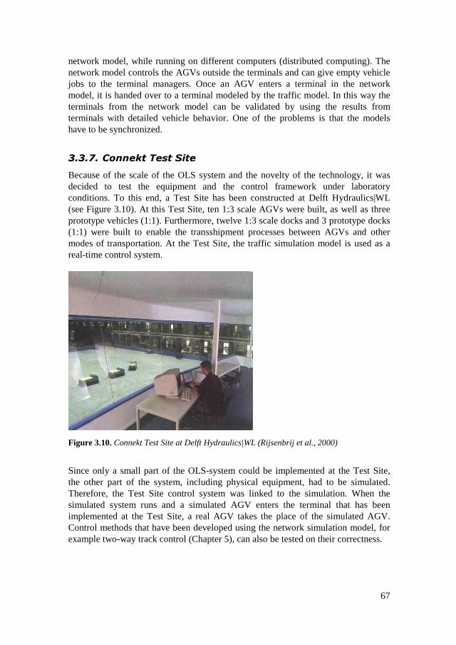
67

network model, while running on different computers (distributed computing). Thenetwork model controls the AGVs outside the terminals and can give empty vehiclejobs to the terminal managers. Once an AGV enters a terminal in the networkmodel, it is handed over to a terminal modeled by the traffic model. In this way theterminals from the network model can be validated by using the results fromterminals with detailed vehicle behavior. One of the problems is that the modelshave to be synchronized.

��6� +��4��3��,��

Because of the scale of the OLS system and the novelty of the technology, it wasdecided to test the equipment and the control framework under laboratoryconditions. To this end, a Test Site has been constructed at Delft Hydraulics|WL(see Figure 3.10). At this Test Site, ten 1:3 scale AGVs were built, as well as threeprototype vehicles (1:1). Furthermore, twelve 1:3 scale docks and 3 prototype docks(1:1) were built to enable the transshipment processes between AGVs and othermodes of transportation. At the Test Site, the traffic simulation model is used as areal-time control system.

Figure 3.10. Connekt Test Site at Delft Hydraulics|WL (Rijsenbrij et al., 2000)

Since only a small part of the OLS-system could be implemented at the Test Site,the other part of the system, including physical equipment, had to be simulated.Therefore, the Test Site control system was linked to the simulation. When thesimulated system runs and a simulated AGV enters the terminal that has beenimplemented at the Test Site, a real AGV takes the place of the simulated AGV.Control methods that have been developed using the network simulation model, forexample two-way track control (Chapter 5), can also be tested on their correctness.

68

'�* !�8�:�79 ( ��7�� :��A�

Important input for the simulation model is the estimated transportation flows. TheOLS system should be able to transport the projected transportation flows of 2020.These projections changed during the project owing to new information andchanging insights. In this section, we describe the various estimates that were usedduring the project and we discuss which data have been used for which part of theresearch.

The estimated transportation volumes for 2020 are translated to transportation units(TU) and were initially estimated by the Netherlands Economic Institute (Table 3.1,CTT 1997). We clearly see an imbalance in these transportation flows; especiallythe route from VBA to RTH is very busy. These transportation flows are used in theexperiments in Chapter 4.

Table 3.1. Estimates in 1997 of the transportation flows in the year 2020 (x1000 TU)

from ↓ to → AAS RTH VBAAAS - 130 50RTH 194 - 177VBA 10 350 -

The project team adjusted the estimates of transportation flows during the project,which resulted in the new transportation flows as shown in Table 3.2. The total flowincreased by about 9%. These transportation flows are the input for the simulationsin Section 6.2 and 6.3.

Table 3.2. Estimates in 1998 of transportation flows in the year 2020 (x1000 TU)

from ↓ to → AAS RTH VBAAAS - 122 67RTH 182 - 197VBA 10 414 -

New changes in transportation flows occurred at the moment the rail terminal wasplanned near Schiphol Airport (cf. Figure 3.3). Transportation flows between the 1st

and 2nd line terminals at Schiphol Airport had to be added. The data for these flowswere obtained from the parties involved at Schiphol Airport. The term AAS stillindicates all terminals at Schiphol Airport, both 1st line and 2nd line. Thetransportation flows were not only estimated for 2020, but also for 2005, 2010 and2015 (Table 3.3). From these flows a growth path can be computed, for example toassess the increasing resource requirements (Van Harten et al., 2000). Thesetransportation flows are input in Chapter 5 and for the evaluation of storage capacityrestrictions in Section 6.4.

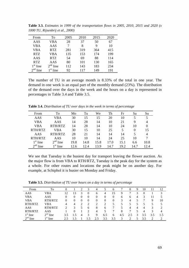
69

Table 3.3. Estimates in 1999 of the transportation flows in 2005, 2010, 2015 and 2020 (x1000 TU, Rijsenbrij et al., 2000)

From To 2005 2010 2015 2020AAS VBA 28 37 50 67VBA AAS 7 8 9 10VBA RTZ 281 319 364 415RTZ VBA 135 153 174 199AAS RTZ 54 69 88 114RTZ AAS 80 101 130 165

1st line 2nd line 112 143 183 2342nd line 1st line 92 117 149 191

The number of TU in an average month is 8.33% of the total in one year. Thedemand in one week is an equal part of the monthly demand (23%). The distributionof the demand over the days in the week and the hours on a day is represented inpercentages in Table 3.4 and Table 3.5.

Table 3.4. Distribution of TU over days in the week in terms of percentage

From To Mo Tu We Th Fr Sa SuAAS VBA 30 15 15 20 10 5 5VBA AAS 14 28 14 10 21 9 4VBA RTH/RTZ 14 28 14 10 24 10 0

RTH/RTZ VBA 30 15 10 25 5 0 15AAS RTH/RTZ 28 21 14 14 14 5 4

RTH/RTZ AAS 10 10 14 24 25 10 71st line 2nd line 19.8 14.8 15.8 17.0 15.1 6.6 10.82nd line 1st line 12.6 12.4 13.9 14.7 19.2 14.7 12.4

We see that Tuesday is the busiest day for transport leaving the flower auction. Asthe major flow is from VBA to RTH/RTZ, Tuesday is the peak day for the system asa whole. For other routes and locations the peak might be on another day. Forexample, at Schiphol it is busier on Monday and Friday.

Table 3.5. Distribution of TU over hours on a day in terms of percentage

From To 0 1 2 3 4 5 6 7 8 9 10 11 12AAS VBA 12 13 3 0 6 4 15 9 7 3 0 1 3VBA AAS 0 0 0 0 0 0 0 6 6 4 3 11 5VBA RTH/RTZ 0 0 0 0 0 0 0 3 4 5 7 9 10RTH/RTZ VBA 4 4 2 2 2 2 5 5 5 5 5 5 5AAS RTH/RTZ 2 3 5 6 8 6 7 5 4 4 4 3 2RTH/RTZ AAS 1 0 1 2 4 5 7 8 7 5 4 3 41st line 2nd line 3.5 1.5 4 3 9 6.5 6 4.5 2.5 3 3.5 3.5 1.52nd line 1st line 2.5 1.5 1 1.5 2.5 3.5 3.5 3 2 5 3.5 2 2

70

From To 13 14 15 16 17 18 19 20 21 22 23AAS VBA 4 0 1 4 0 0 0 4 10 1 0VBA AAS 16 16 5 1 0 1 16 4 6 0 0VBA RTH/RTZ 7 6 5 6 9 9 9 6 4 1 0RTH/RTZ VBA 5 5 5 5 5 4 4 4 4 4 4AAS RTH/RTZ 2 3 4 5 6 5 5 4 3 3 1RTH/RTZ AAS 3 5 3 2 3 5 7 7 6 4 41st line 2nd line 1 3 1.5 2.5 3 6 8 4 2.5 8 8.52nd line 1st line 6.5 4.5 10.5 11.5 6.5 4 2.5 2.5 9.5 4 4.5

The transportation flows are also distributed very unevenly over the day. On mostroutes it is rather quiet during the night and early morning. There are two peaks onthe busiest route, from VBA to RTH/RTZ, one around noon and another around18:00. It turns out that these peaks determine the system performance to a largeextent. All routes have their own peaks, mostly at different times of the day. Giventhe transportation flows on the different routes, the demand distribution in anaverage month or week can be easily derived from these figures.

The transportation flows are not uniformly distributed over the 1st and 2nd lineterminals. These flows have to be separated into four different flows. Thedistribution of the internal transportation flows at Schiphol over 1st and 2nd lineterminals, and the distribution of the transportation flows between Schiphol andRTZ, and Schiphol and VBA. These distributions are represented in the followingtables, and were obtained from interviews with the parties involved. When terminalsare not mentioned, the corresponding percentages are equal to 0.

Table 3.6. Distribution of internal transportation flows at Schiphol over 1st line terminals in2020 in terms of percentage

1st line Export ImportTerminal 2nd -> 1st line 1st -> 2nd line

5 0.0% 58.1%6 24.3% 0.0%7 24.3% 0.0%

12 20.9% 15.2%14 4.8% 8.0%15 25.7% 18.7%

Table 3.7. Distribution of the internal transportation flows at Schiphol over the 2nd lineterminals in 2020 in terms of percentage

2nd line Export ImportTerminal 2nd -> 1st line 1st -> 2nd line

1 2.6% 5.0%2 12.9% 19.3%3 12.9% 19.3%4 12.9% 19.3%8 20.7% 22.8%9 38.0% 14.3%

71

The internal transportation flows at Schiphol from a 1st line terminal to a 2nd lineterminal can now be computed as follows. The total volume (Table 3.3) has to bemultiplied by the percentage of the export flow at the 1st line terminal and thepercentage import at the 2nd line terminal. We assume that these distributions areindependent. The flow from 2nd line to 1st line terminals can be computed similarly.Table 3.8 shows the percentage of the flow to other locations.

Table 3.8. Distribution of transportation flows between AAS and VBA, and AAS and RTZover the AAS terminals in 2020 in terms of percentage

Terminal AAS-VBA VBA-AAS AAS-RTZ RTZ-AAS

5 0.0% 0.0% 32.0% 0.0%6 0.0% 37.5% 0.0% 18.25%7 0.0% 37.5% 0.0% 18.25%

10 0.0% 0.0% 2.2% 2.3%11 0.0% 0.0% 8.9% 6.4%12 40.0% 25.0% 23.1% 22.3%14 20.0% 0.0% 5.3% 5.1%15 40.0% 0.0% 28.5% 27.4%

Note that not all terminals at Schiphol will be used in 2020. Some of the terminalswill be used until 2010 and then replaced by other terminals that have not yet beenbuilt.

For the transportation flows we use the following arrival processes in oursimulations:• Poisson arrivals at AAS and VBA, with the average number of arrivals

depending on the time of day.• Batch arrivals at RTH/RTZ (train station), with an average number of arrivals

dependent on the time of day. At first we assume that the number of trains perhour is uniformly distributed between 2 and 4, with fixed inter-arrival times(Chapter 4 and 6). Later on we chose 6 train arrivals per hour, also with fixedinter-arrival times (in the case of a rail terminal at Schiphol Airport, Chapter 5and Section 6.4). The number of loads per train is Poisson distributed.

All transportation jobs that are generated in the system have to be executed, evenwhen they are late, because the order acceptance procedure has already been passed.The dimensioning and performance measurement will be done for a peak day in anaverage month (Tuesday). We assume that transportation jobs are known 30 minutesbefore arrival at the terminal of origin. This is a reasonable assumption for ourapplication because plane and train arrivals are known a long time before the actualtime of arrival. This information can be used in the different planning methods. Insome experiments this information horizon is an experimental factor.

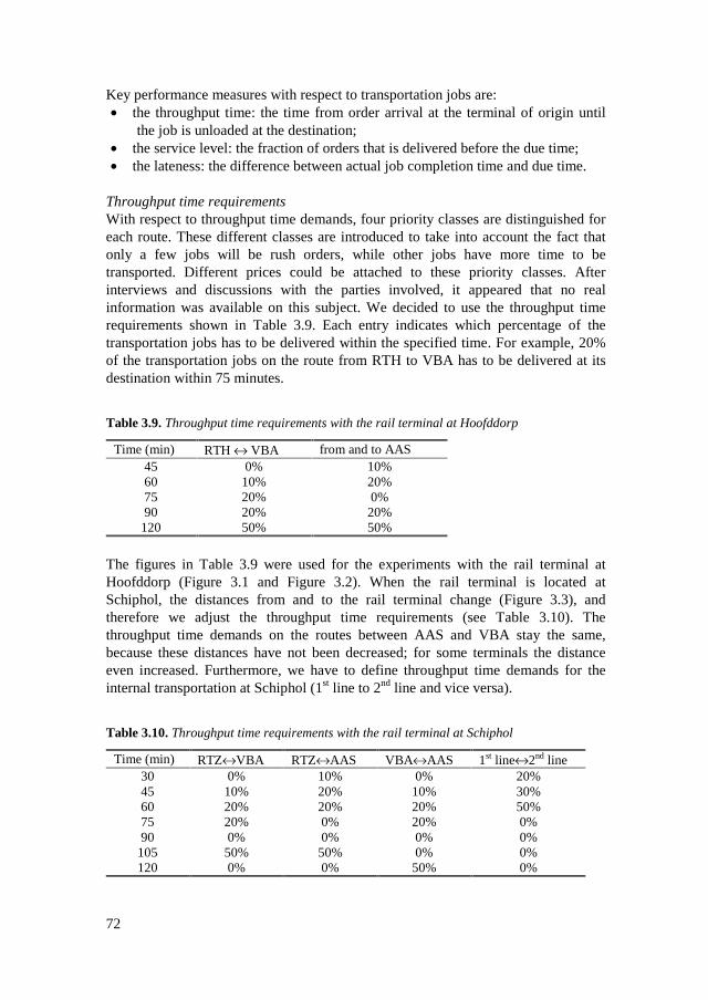
72

Key performance measures with respect to transportation jobs are:• the throughput time: the time from order arrival at the terminal of origin until

the job is unloaded at the destination;• the service level: the fraction of orders that is delivered before the due time;• the lateness: the difference between actual job completion time and due time.

Throughput time requirementsWith respect to throughput time demands, four priority classes are distinguished foreach route. These different classes are introduced to take into account the fact thatonly a few jobs will be rush orders, while other jobs have more time to betransported. Different prices could be attached to these priority classes. Afterinterviews and discussions with the parties involved, it appeared that no realinformation was available on this subject. We decided to use the throughput timerequirements shown in Table 3.9. Each entry indicates which percentage of thetransportation jobs has to be delivered within the specified time. For example, 20%of the transportation jobs on the route from RTH to VBA has to be delivered at itsdestination within 75 minutes.

Table 3.9. Throughput time requirements with the rail terminal at Hoofddorp

Time (min) RTH ↔ VBA from and to AAS45 0% 10%60 10% 20%75 20% 0%90 20% 20%

120 50% 50%

The figures in Table 3.9 were used for the experiments with the rail terminal atHoofddorp (Figure 3.1 and Figure 3.2). When the rail terminal is located atSchiphol, the distances from and to the rail terminal change (Figure 3.3), andtherefore we adjust the throughput time requirements (see Table 3.10). Thethroughput time demands on the routes between AAS and VBA stay the same,because these distances have not been decreased; for some terminals the distanceeven increased. Furthermore, we have to define throughput time demands for theinternal transportation at Schiphol (1st line to 2nd line and vice versa).

Table 3.10. Throughput time requirements with the rail terminal at Schiphol

Time (min) RTZ↔VBA RTZ↔AAS VBA↔AAS 1st line↔2nd line30 0% 10% 0% 20%45 10% 20% 10% 30%60 20% 20% 20% 50%75 20% 0% 20% 0%90 0% 0% 0% 0%

105 50% 50% 0% 0%120 0% 0% 50% 0%

73

'�) �7 :=:B� :��;��9��:=9� :��(�� :=� :�� 6��9��C9:��=��

One of the issues in the pre-design phase of the project was the estimation ofresource capacities required to handle the projected cargo within the throughput timelimits as specified in the previous section. Although the simulation model may beused, one may wonder whether it is possible to develop an analytical model for thispurpose. In this section, we show that such a model can be constructed for somecases. However, it appears that some system layouts (those including one or moretwo-way tubes) are difficult to analyze analytically. For those cases, simulation isthe only feasible alternative.

We first present an analytical model to estimate capacity requirements (AGVs,docks) for the Stommeer layout (see Figure 3.1). The ideas of Maxwell andMuckstadt (1982) are used, but in addition time is taken into account. Obviously, theopportunities for peak shaving influence capacity requirements, because theworkload fluctuates strongly over time (see Table 3.4 and Table 3.5). If the dispatchtime window for the jobs increases, the effective peak demand decreases and fewerAGVs and docks are required to handle the cargo flows. This aspect is part of ourmodel.

We compare the estimates from this model with the simulation results. For the othersystem designs we only present the resource requirements derived from thesimulation experiments. In order to be able to determine the resource requirements,we have to know the maximum transportation flows in a given time interval in amore-or-less steady state. Once these steady state flows are known, there should besufficient resources (AGVs and docks) to handle these flows.

��5�� 7�� #��

We present an analytical model for a network with deterministic travel times (cf.Section 1.3.2). In this model the transportation flows are spread over the timeintervals, termed peak shaving, to level the workload in the different time intervals.The possibilities for peak shaving are limited by the throughput time requirements.Furthermore, the empty vehicle flows, necessary to reposition the vehicles becauseof the imbalance in transportation flows, are estimated. Time is modeled in discretetime intervals, t ∈ {0,…,T}. First we assume that all transportation jobs that arestarted in time interval t will also be delivered within that same time interval, laterwe leave this assumption. To keep the model solvable, the number of time intervalsshould not be too large. A time interval of 1 hour seems reasonable for ourapplication. First, we introduce some notation:M = set of terminals, indexed by i and jτij

l = handling times, the total time required for handling one transportation job,i.e. the loading time, driving time to the exit of terminal i, driving time toterminal j, driving time from terminal entrance to a dock, and the unloadingtime (in minutes).

74

τije = empty driving time, that is the driving time to the exit of terminal i, the

driving time to terminal j, and the driving time on terminal j toward a dock(in minutes).

fijt = transportation flows, the number of TU that has to be transported fromterminal i to terminal j, with order release time at terminal i in interval t.

aijts = shift parameters, s ∈ {0,1,2,…}, the percentage of transportation jobs fromterminal i to terminal j, that arrives in time interval t at terminal i and has tobe dispatched within s time intervals after arrival. This is a cumulativepercentage, i.e. aijts ≥ aijts-1. For simplicity we assume that the aijts areindependent of t, as is the case in the OLS, see Table 3.12. For example, aij1

is the percentage of the transportation jobs that arrives in time interval t andthat has to be dispatched before the end of time interval t+1.

Decision variables:xijt = the number of transportation jobs from terminal i to terminal j started in

time interval t.yijt = the number of empty trips between terminal i and terminal j started in time

interval t.αijts = percentage of transportation jobs that arrived in time interval t, and is

dispatched in time interval t+s.

The required number of AGVs N(t) can be estimated from the total driving timebetween terminals plus the total time spend at terminals. We have to look at timeinterval t*, in which the maximum amount of AGV time is required. The requirednumber of AGVs is:

( )60

)(∑∑ ∑ ⋅+⋅+⋅

= i j i

iqi

eijijt

lijijt Wyx

tN

λττ (1)

and t* = arg max N(t). Here λi denotes the dock operations intensity at terminal i andWq

i the waiting time at terminal i for one dock operation. The time spent on aterminal is subdivided in the time for driving, the loading and unloading time andthe waiting time. The driving time on the terminal and the loading and unloadingtime are included in the handling time (τij

l) and the empty driving time (τije). Waiting

times at docks occur owing to the limited dock capacity. Once the number of dockoperations in time interval t at terminal i is known ( ∑∑ +=

j jitj ijti xxλ ), the

expected waiting time for one dock operation (Wqi) can be approximated using a

standard multi-server queuing model.

Model:In our model we ensure that the transportation flows are distributed over the timeintervals in order to minimize the maximum workload in an interval for AGV

75

driving time plus the docking time. Hence, waiting time is introduced as a correctionafterwards. The objective function is:

( )

⋅+⋅∑∑i j

eijijt

lijijt

tyxMaxMin ττ (2)

Subject to:

tjis

ijts ,,1 ∀=∑α (3)

stjiaijssk

ijtk ,,,∀≥∑≤

α (4)

tjifxtkk

ktijkktijijt ,,,0

,,, ∀⋅= ∑<≥

−−α (5)

( ) ( ) tiyxyxj

jitjitj

ijtijt ,∀+=+ ∑∑ (6)

tjixijt ,,integer,,0 ∀≥ (7)

tjiyijt ,,integer,,0 ∀≥ (8)

Constraint (3) indicates that the sum of the fractions should be equal to 1.Postponing transportation jobs to later time intervals is limited by the throughputtime requirements (4). The number of loaded trips in one time interval is equal to thetransportation jobs that are postponed from the previous time intervals plus thepercentage of transportation jobs that arrive in the current time interval and are alsodispatched in the current time interval (constraint 5). The first three constraintsspread the total workload over the different time periods (peak shaving). Constraint(6) includes the conservation of flow constraints. All flows have to be nonnegativeintegers (constraint 7 and 8). In this formulation we assign handling times to thetime interval in which the job is started. Note that this formulation does notnecessarily minimize the empty trips. The objective is to minimize the maximumworkload in a time interval. In quiet time intervals unnecessary empty trips may beplanned, without affecting the objective function. Additional constraints can beadded to also minimize empty trips outside the peak periods. However, this is notthe focus of our model.

To solve the problem the objective function is transformed to constraint (9), with anobjective function to minimize C:

( ) tCyxi j

eijijt

lijijt ∀≤⋅+⋅∑∑ ττ (9)

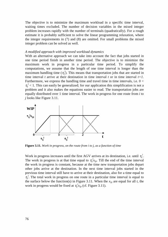
76

The objective is to minimize the maximum workload in a specific time interval,waiting times excluded. The number of decision variables in the mixed integerproblem increases rapidly with the number of terminals (quadratically). For a roughestimate it is probably sufficient to solve the linear programming relaxation, wherethe integer requirements in (7) and (8) are omitted. For small problems the mixedinteger problem can be solved as well.

A modified approach with improved workload dynamicsWith an alternative approach we can take into account the fact that jobs started inone time period finish in another time period. The objective is to minimize themaximum work in progress in a particular time period. To simplify thecomputations, we assume that the length of one time interval is longer than themaximum handling time (τij

l). This means that transportation jobs that are started intime interval t arrive at their destination in time interval t or in time interval t+1.Furthermore, we express the handling time and travel time in time intervals, i.e. 0 <τij

l < 1. This can easily be generalized; for our application this simplification is not aproblem and it also makes the equations easier to read. The transportation jobs areequally distributed over 1 time interval. The work in progress for one route from i toj looks like Figure 3.11.

t

WIP

210ij

lij

l

ijlxijt

Figure 3.11. Work in progress, on the route from i to j, as a function of time

Work in progress increases until the first AGV arrives at its destination, i.e. until τijl.

The work in progress is at that time equal to τijlxijt. Till the end of the time interval

the work in progress is constant, because at the time new transportation jobs departother jobs arrive at the destination. In the next time interval jobs started in theprevious time interval still have to arrive at their destination, also for a time equal toτij

l. The total work in progress on one route in a particular time interval is equal tothe surface below the function(s) in Figure 3.11. When the xijt are equal for all t, thework in progress would be fixed at τij

lxijt (cf. Figure 3.11).

77

The objective function is:

( ) ( ) ( ) ( ){ }

++−+−∑∑= =

−−

M

i

M

jtij

eijtij

lijijt

eij

eijijt

lij

lij

tyxyx

1 11,

2

21

1,

2

21

21

21 11maxmin ττττττ (10)

With flow conservation constraints:

( ) ( ){ } { } tiyxyxyxM

j

M

jijtijtjit

ejijit

ljijit

ejijit

lji ,11

1 1

∀+=−+−++∑ ∑= =

ττττ (11)

The other restrictions, (3)-(5), (7) and (8) still apply. Owing to these flowconservation constraints, we can no longer solve the problem as a mixed integerproblem (cf. constraint 6); we have to solve a linear programming relaxation. But inany case the model is only used to obtain a rough estimate of the required resources.Furthermore, experiments with the formulation in equations (2)-(8) show that theinteger solution is within 1 percent of the linear programming relaxation. Theformulation in equations (10) and (11) can be extended to smaller time intervals, τij

l

> 1, using a similar approach. The driving time can be longer than 1 time interval,which leads to additional terms in equation (10) and (11). Because we are onlysearching for a rough estimate, we do not discuss this extension here.

Determining the aijs

The aijs are determined using the throughput time requirements (see Section 3.4).We assume that the length of a time interval is one hour. When a specifictransportation job arrives, which has a required throughput time of 60 minutes andrequired handling time (τij

l) of 30 minutes, the time window for starting thistransportation job is 30 minutes. When the job arrives in the first half-hour, the jobhas to be transported within that same hour, while the job can be postponed to thenext hour if it arrives in the second half-hour. For example, given a total number of140 transportation jobs on a particular route, 70 jobs cannot be postponed to the nexthour and 70 jobs can be postponed: a0=0.5 and a1=1. These computations can beexecuted for all routes. In the OLS-case, the transportation jobs always have to betransported within the next two hours after the hour of arrival (s ≤ 2). The larger aij0,the less possibilities for peak shaving.

Determining the required number of docks from the maximum dock utilizationThe xijt, computed with one of the two formulations presented, can now be used in aqueuing model to determine the required number of docks at each terminal. Forthese computations, we assume that the AGVs and transportation jobs arrive atterminal i according to a Poisson distribution (simplification of the OLS-case) with

mean arrival rate }{max ∑∑ +=j jitj ijt

ii xxλ , the maximum number of dock

operations in one time interval. For simplicity, we assume that the loading andunloading times are also exponentially distributed, with µi the possible number of

78

dock operations per dock per time interval at terminal i. For such an M/M/s queue, inwhich s represents the number of docks, the utilization rate is defined as:

ii

ii s µ

λρ =

To ensure that the steady-state probabilities exist this utilization rate should besmaller than 1. Given a maximum dock utilization ρ (e.g. 0.8), we can compute theminimum required number of docks at terminal i, Nd,i.

=

ii

iidN

µρλ

, , where x denotes the smallest integer that equals or exceeds x.

Given the number of docks, si, the expected waiting time per dock operation followsimmediately. The average time an AGV waits in line at terminal i is (Winston,1991):

i

iqi

q

LW

λ=

with i

iiiq

smPL

ρρ

−≥

=1

)(,

)1(!

)()( 0

ii

sii

i s

ssmP

i

ρπρ

−=≥

∑ −== −

+=

1

0

0

)1(!

)(

!

)(

1

i

isk

kii

sii

kii

s

s

k

s

ρρρ

π

These waiting times can also be computed for time interval t*, and used in thecomputation of the required number of AGVs (equation 1). If desired the number ofdocks can be determined using the expected waiting time for a dock operation as aconstraint, see the discussion following Table 3.13.

��5�� 8/ ��9�,�� #��

We apply the model with equations (2)-(8) from the previous section to theStommeer layout (Figure 3.1), with the transportation flows from Table 3.1 andcorresponding throughput time requirements. Because the transportation flows aredefined per location (VBA, RTH and AAS), we use these locations in the analyticalmodel. The average empty travel times between the locations, given an AGV speedof 6 m/s, are shown in Table 3.11. We assume that the average dock operation timeis equal for loading and unloading and for all terminals, and equals 2 minutes. Thedriving time on the terminal is equal to 0.8 minutes for VBA, 0.4 minutes for AASand 1.2 minutes for RTH.

79

Table 3.11. Average travel time between the locations in minutes (6 m/s)

VBA RTH AASVBA 0 26.2 23.2RTH 26.2 0 20.1AAS 23.5 21.4 0

In Table 3.12 we show the shift parameters aijs, derived from the throughput timerequirements. Notice that only a small percentage concerns rush orders, which haveto be transported almost immediately.

Table 3.12. The shift parameters for the different routes (aijs)

route aij0 aij1 aij2

VBA-RTH 0.11 0.76 1RTH-VBA 0.11 0.76 1VBA-AAS 0.16 0.72 1AAS-VBA 0.16 0.72 1RTH-AAS 0.15 0.70 1AAS-RTH 0.15 0.70 1

The length of a time interval is 1 hour; T is equal to 24. We will address the peakday (Tuesday) in an average week. The model is terminated after finding the optimalsolution or when no improvements in the objective function have been found in 30seconds. The model was implemented in AIMMS (using the XA solver).

DocksThe model of equations (2)-(8) results in λ1 =180, λ2 =230, and λ3 =90. We assumethat the number of dock operations, λi, is equally distributed over the number ofterminals of location i, so a different M/M/s queue for each terminal (2 at VBA and5 at AAS). In Table 3.13 we show the mean waiting times in minutes and utilizationrates for the different locations and different number of docks (s).

Table 3.13. Expected waiting times and the dock utilization rates (between parenthesis)

s=1 s=2 s=3 s=4 s=5 s=6 s=8 s=9 s=10 s=11VBA 1.42 0.27 0.07

(0.75) (0.6) (0.5)RTH 23.6 1.41 0.39 0.15

(0.96) (0.85) (0.77) (0.7)AAS 9.12 0.45 0.05

(0.6) (0.3) (0.2)

The dock utilization rate (ρ) can be misleading when used in determining therequired number of docks. One could assume that 1 dock per AAS terminal issufficient, but the expected waiting time for a dock operation in the peak hour ismore than 9 minutes. Because we do not want the docks to be a bottleneck, wechose 2 docks per AAS terminal, 5 docks per VBA terminal and 10 docks at RTH.

80

AGVsIn determining the required number of AGVs we find λ1

* =180, λ2

* =230, and

λ3*=50, also equally distributed over the terminals at one location. Notice that in this

particular time interval the AAS terminals are not at their peak capacity. After fillingin equation (1), the required number of AGVs is 165. The second approach, usingequations (10) and (11) instead of (2) and (6), results in a required number of AGVsof 163. Recall that this is the solution of the linear programming relaxation.

It is interesting to look at the contribution of each activity to the total number ofrequired AGVs. The different contributions give an indication of the influence of thespeed of the AGV and the loading and unloading times of docks. An increase inAGV speed could reduce the number of required AGVs considerably when there arelong distances between the terminals. At a speed of 10 m/s the estimated number ofAGVs is 108, at 15 m/s the estimate is 81 AGVs. In these experiments we used thesame intermediate distance between AGVs (3.5 seconds). When the intermediatedistance increases the reduction in AGVs is smaller. The estimate for the requirednumber of AGVs is more-or-less a lower bound. In reality the transportation jobswill not be spread uniformly over the time interval and the peak shaving will alsonot be perfect. Comparison with simulation results in the next section shows thatthis leads to significant effects.

��5�� #��

Extending the analytical model to systems with two-way tracks is difficult. Thetravel times are no longer deterministic, and long waiting times occur at the two-way tracks. Especially these waiting times at the two-way tracks, and resultingwaiting times at terminals due to convoy arrivals are difficult to estimate. For thesekinds of systems simulation has proven its value. Simulation experiments candetermine the resource requirements rather easily. The sensitivity of the system toparameters such as AGV speed and docking speed might be even greater with two-way track sections. Other parameters, such as the intermediate distance betweenAGVs and the acceleration and deceleration of AGVs also influence the resourcerequirements. The results of the simulation study are shown in Table 3.14.

Table 3.14. Resource requirements from the simulation model

Layout AGVs docksRTH/RTZ

docksVBA

docks AAS

Stommeer 185 10 2x5 5x2Two-way tubes 360 8 8 3x2Internal transport Schiphol 250 8 8 18x2

The required number of docks for the Stommeer layout is equal to the estimates ofthe analytical model. The required number of AGVs in the simulation is about 12%more than estimated by the analytical method. This is not really surprising, becausethe transportation jobs are not equally distributed over a time interval due to the

81

stochasticity and batch train arrivals, and the peak shaving will not be perfect.Another reason is that the planning of the AGVs will not be optimal, partly due toincomplete information and stochasticity in the travel times. We also see that theintroduction of two-way tracks, plus some other modifications, significantlyincreases the required number of AGVs. Most of these additional AGVs are requiredbecause of the waiting times at the two-way tracks and, as a result of the convoyscreated, the waiting times at the terminals. Moving the rail terminal to Schipholclearly reduces the required number of AGVs, because of shorter distances, but thenumber of terminals at Schiphol increases considerably.

'�0 ��9�:��

From the previous section we can conclude that analytical methods are only usefulfor particular sub-problems, such as the determination of the required number ofAGVs, and then only in case of nearly deterministic travel times. As was discussedin Chapter 1, a simulation model seems the only way to incorporate all features ofthe model.

The simulation group appeared to be important in the pre-design phase of the OLS-project. The simulation group received a lot of input from the other research areas,as described in Section 3.3. The simulation model could determine the logisticalconsequences of the technological ideas from several other groups. An example isthe question of whether the use of two-way tubes is feasible from a logistic point ofview. Simulation experiments showed that two-way tubes could be used, but withserious consequences on the logistic performance and resource requirements.Furthermore, simulation results were important input for the energy study (Van derHeide, 1999) and cost analyses of the different system layouts.

In the experiments in the following chapters the AGV specifications, as described inSection 3.3.3, will be used, with a required time between two AGVs of 3.53 secondsand with the speed on the terminal equal to (2-0.024N) m/s, as was derived in thetraffic simulation model. The Stommeer layout from Figure 3.1 is used for theexperiments in Chapter 4, with terminals similar to the one shown in Figure 3.5 andan average docking time equal to 2 minutes. These experiments are based on thetransportation flows in Table 3.1. The layout with two-way tubes (Figure 3.2) isused in Chapter 6, with terminals similar to the one shown in Figure 3.5 and anaverage docking time equal to 1 minute. The transportation flows from Table 3.2 areused for these experiments. The layout with the rail terminal at Schiphol (Figure 3.3)is used in Chapter 5 and in Section 6.4, with the small Schiphol terminals as shownin Figure 3.7, the VBA terminal similar to Figure 3.5, and a rail terminal withoutshortcuts and parking places. The average docking time is 1 minute and thetransportation flows are shown in Table 3.3. This layout was also used to compute agrowth scenario for the years 2005-2020, see Van Harten et al. (2000).

83

�6�7 ��

*

�� 6�7�:=��?7��(;�6:��=��<�=��

*�� 89� :��

In this chapter we discuss various options for empty vehicle management, i.e. thepre-positioning of empty vehicles in the network to anticipate known and predicteddemand. The need for empty vehicle management is inevitable becausetransportation flows will generally be unbalanced over time; the number of vehiclesarriving in a time interval at a terminal differs from the number of vehicles to beloaded and dispatched in the same interval and from the same terminal. Emptyvehicle management is especially critical in situations where due times are tight andresource utilization (vehicles, docks) is high. The scheduling of empty AGVs isclosely related to the scheduling of transportation jobs. Transportation jobs requireempty AGVs and finished transportation jobs result in empty AGVs. Therefore wewill study the planning of both empty and loaded vehicle travel. We consider severalplanning options in which the required information and the level of coordination arevaried. We are especially interested in the following subjects:• How do look-ahead policies compare to simple myopic planning rules?• What is the value of information about future transportation jobs?• To what extent can central coordination contribute to a more efficient system

compared to decentralized planning and control?

2 This chapter is partly based on Van der Heijden et al. (2001a).

84

These issues will be discussed for general transportation networks. The OLS projectserves as a test case. We will use the model developed in Chapter 2 to test andevaluate the various options for empty vehicle management. All other controlactivities besides vehicle management, such as task allocation to docks and vehiclecontrol, will be controlled according to the descriptions in Chapter 2.

The remaining part of this chapter is organized as follows. In the next section, wediscuss an integer linear programming and a dynamic programming formulation forthe vehicle management problem. An overview of related literature is given inSection 4.3. Various options for empty vehicle management without centralcoordination are introduced in Section 4.4. In Section 4.5 we present a serialscheduling approach to solve the vehicle management problem. A large part of thischapter is devoted to a logistic queuing network approach, which is described inSection 4.6. Note that this is a queuing network as defined by Powell and Carvalho(1998a), which is not exactly the same as other queuing networks encountered in theliterature. The simulation study with numerical results based on the OLS-case, is thesubject of Section 4.7. We summarize our main conclusions in Section 4.8.

*�� !�8��8��9=7 :��

In this section we describe an integer linear programming and a dynamicprogramming formulation for the vehicle management problem. First, we present adiscrete model as proposed by Powell and Carvalho (1998a). We assume that time isdivided into a set of discrete time periods t = (1,...,T). T is the planning horizon intotal number of time periods. All time-related activities, such as travel times andloading/unloading times have to be transformed into discrete time periods. First wepresent the notation for the problem.

Network variables:• M is the set of terminals and parking areas, indexed by i and j (for simplicity we

will mainly talk about terminals in the remainder of this chapter, but parkingareas are included)

• τije is the expected empty travel time from terminal i ∈ M to terminal j ∈ M,

τiie =1, τij

e > 0; all travel times are positive• τij

l is the expected handling time from terminal i ∈ M to terminal j ∈ M, τijl > 0

(from the start of the loading operation until the end of the unloading operation,travel time included)

• N is the set of nodes (i,t) in the dynamic network, i ∈ M and t ≤ T

The expected travel times and handling times will be estimated using the methodsdescribed in Section 2.6.

85

Parameters:• rlt is the revenue generated by choosing time t to start transportation job l• cijt is the cost of repositioning one empty vehicle from terminal i to terminal j,

starting in time period t.• Tl is a discrete interval, which contains all the feasible time periods for starting

transportation job l ∈ L, otherwise known as the departure time window.• Tl

s is the first time period of the departure time window Tl of transportation jobl.

Activity variables:• L is the set of transportation jobs l available within the planning horizon T, i.e.

the release time of order l is contained in the planning horizon.• Lijt is the set of transportation jobs l ∈ L with origin i and destination j, having t

as a feasible departure time.• RVit is the net inflow (RVit > 0) or outflow (RVit < 0) of vehicles at terminal i at

time t.

Decision variables:• xlt = 1 if transportation job l is started at time t, xlt only exists for t ≥ Tl

s.• yijt is the number of empty vehicles being repositioned from terminal i to

terminal j at time t. yiit is the number of vehicles, which is kept in inventory atterminal i from time period t to time period t + 1.

�� .��

The problem can be formulated as an integer linear program (P1), for the periods t =1,…,T. Our problem consists of maximizing profit by assigning one vehicle to eachtransportation job, and enforcing conservation of flow at each node.

∑∑∑ ∑= ∈ ∈ ∈

−=

T

t Mi Mj Llijtijtltlt

ijt

ycxryxFyx 1

),(,

max (1)

Subject to:

Llxs

lTtlt ∈∀=∑

≥1 (2)

NtiRVyxyx tiMj

tijLl

tlMj

ijtLl

lt eji

jit

lji

ijt

∈∀=

+−

+ ∑ ∑∑ ∑

∈−

∈−

∈ ∈),( ,,,, ττ (3)

][1,..., }1,0{ TtLlxlt ∈∀∈∀= (4)

][1,..., , integer 0 TtMjiyijt ∈∀∈∀≥ (5)

The objective function (1) maximizes the revenues, which can be separated into thepositive revenue of a loaded move (rlt) and the negative revenue (costs) of an emptymove (cijt). We need to sum these terms over all the possible movements and all the

86

time periods. The first constraint (2) deals with the fact that all the transportationjobs have to be transported. This means that the variable xlt has to be equal to 1 onlyonce, because the start of transportation job l can only take place in one time period.To start transportation job l, it has to be available at the terminal of origin.Therefore, the time period t has to be greater than or equal to the time period of thearrival of order l at the terminal (Tl

s). Because all transportation jobs have to betransported, there is no latest starting time. Nevertheless, the revenue function canbe related to the due time of the transportation job. Constraint (3) has to deal withthe flow of AGVs in the system. Flow conservation constraints must be present.However, we can also have a flow into terminal i in time period t as a result of theinitial system state, in which AGVs are driving between terminals and arrive at aterminal during some future time period. This flow is called RVit. Since the first partof the right hand side of this equation only refers to the present planning horizon t -τij

l ≥ 1 and t - τije ≥ 1. For an arbitrary period t, we see that at terminal i, the

incoming flow is equal to the outgoing flow. The last two constraints are integralityconstraints.

The model focuses on revenue maximization, whereas we are mainly interested inminimizing lateness. The formulation of the model can easily be adjusted to anotherobjective. To this end, we use the following definitions:dl = the due time of job l (input data)alt = the lateness of job l if it is started at time tThe lateness of each job, depending on the starting time t, can be calculated as

{ }0, llijlt dtMaxa −+= τ

Hence the minimization of the total lateness can be formulated as

∑∑ ∑ ∑= ∈ ∈ ∈

=

T

t Mi Mj Llltlt

xijt

xaxF1

)(min

Alternatively, we can formulate the objective to minimize the maximum lateness as

ltltTtLlx

xaxF≤≤∈

=1,

max)(min

To obtain the optimal solution of the problem, a branch-and-bound approach can beused, possibly based on the linear programming relaxation (if the objective isrevenue maximization or total lateness minimization). What makes this problem socomplex is not only the presence of the integer variables, but also the fact that theproblem has to be solved over an extended planning horizon. Because of themagnitude of the problem, problems like this also result in an intractably largeinteger (linear) program, which takes little advantage of the dynamic structure of thesystem. Maximizing the total revenue can be equal to minimizing the total lateness

87

if all cijt are equal to 0. The revenue function should penalize lateness and could looklike rlt = R-alt, with R the revenue for delivering a transportation job on time (cf.Section 4.6.5).

�� #� ��

Besides formulating the problem as an integer linear program, we can also formulateit as a dynamic programming problem (DP). Here we give a possible formulation.The state consists of: Rk

i, el. Here i, j ∈ M refer to the terminals, k ∈ {1,…,τ},indicates a future time period that can be influenced by the decision at time t, withτ = max{τij}, an upper bound on the travel time between two terminals. Furthermore,l ∈ tL , the set of jobs that is available for transport at time t, but that has not yet

been moved. itL is the subset of tL , only including those jobs with terminal i as

origin. The interpretation of the state variables is as follows:• Rk

i = the number of empty vehicles that comes available at terminal i, k periodsahead if no further action is taken.

• el = the earliness of job l, from terminal i to terminal j, if it is executed in thecurrent time interval t: dl – (t+τij

l).

Note that R0i at decision moment t is equal to Vit defined in Section 4.6.1 and

∑ ki

ikR

,is equal to the total number of vehicles. As a shorthand notation for the state

we use {R,e}.

Decision variables at decision moment t:xlt = {0,1}, indicating whether job l, corresponding with el, is scheduled in thecurrent decision period.yijt = number of empty vehicles moved from terminal i to terminal j.

All vehicles need to be assigned to a job, possibly a job on the current terminal:yiit > 0. Thus, by definition:

iyxRj

ijtLl

lti

it

∀+= ∑∑∈

,0

The direct costs, given state {R,e} and decision {x,y}, can be separated into:1) Direct costs for lateness: ∑

∈<=

t

lLl

eIC

}0{1 , with I the indicator function.

2) Direct costs for empty moves from terminal i to terminal j, with i≠j:

∑≠

=jiji

ijtyC,,

2 . If there are non-capacitated terminals we associate no costs with

waiting empty at a terminal.3) Direct rewards from the execution of transportation jobs: ∑

∈=

tLlltxW3

88

It is possible to consider more general cost functions, for example:

∑=ji

ijtijt ycC,

2 and ∑∈

=tLl

ltlt xrW3 ,

with cijt the costs of an empty move from terminal i to terminal j at time t, with t adecision moment, and rlt the revenue of executing transportation job l at time t.These functions are comparable to the ones used in Section 4.6.1. In this formulationdirect costs are associated with lateness, which in equation (1) can be incorporatedin the revenue function rlt. If desired, other cost components can be introduced, forexample for exceeding the terminal capacity. The structure of equations (2) and (3)could also be generalized, but we consider the simple form as given.

The state transition from {R,e} at time t to }ˆ,ˆ{ eR at time t+1, given decision {x,y},

looks like:

a) ∑∑∑∑ −−++=∈==∈ j

ijtLl

ltj

jitLl

ltii yxyxRR

jteji

ljijt 1,1,

10ˆ

ττ; the vehicles that arrive due to

previous decision moments, plus the vehicles that arrive due to currentdecisions at other terminals, minus the vehicles that leave the terminal givendecision {x,y}. Recall that τij

e>0 and τiie=1.

b) ∑∑+=+=∈

+ ++=1,1,

1ˆ

kjjit

kLllt

ik

ik

jijijt

yxRRττ

, for k < τ, where we define Rτi=0.

c) In e we omit all elements from e for which xlt=1.

d) 0 with 1ˆ =∈∀−= lttll xLlee ; the jobs that were not planned get closer to

their due times (possible lateness increases).e) The set 1+tL is constructed from the jobs of set tL with xlt equal to 0, plus the

jobs that are released at the start of time interval t+1.f) For each job that is released at time t+1 we create (iteratively) a new l’, and we

define )1(ˆ ’’lijll tde τ++−= .

We define the value function Gt{R,e} as the minimum costs over [t,T], given state{R,e} at the beginning of time t. The overall DP objective is to minimize G1 giventhe initial state {R,e}. The recursion relation then looks as follows:

{ }}ˆ,ˆ{)()()(max},{ 1321,

eRGxWyCeCeRG tyx

t +++−−= (6)

Before we can solve the DP, we have to define the end values for state {R,e} at timeT. First, we consider the lateness costs. Let us introduce the notation:

}0{0 >= li exn , the number of jobs already late at terminal i at time T

}1{ −== kexn lik , the number of jobs that become late in period T+k at terminal i.

89

Then it is clear, that at least the following lateness costs are generated at terminal iat time T:

for k=0: i

def

i Sn 00 =

for k=1: ( ) i

def

iii SRnn 1010 0,max =−+

for k=m: im

def

m

p

ip

m

p

ip

i SRnn =

−+ ∑∑

−

==0,max

1

010

The lateness costs consist of the transportation jobs that are already late at time Tplus the jobs that cannot be transported in time by the number of vehicles thatarrives in future time periods. Hence, the lateness costs are at least:

∑=i

iiKSC )(1

with K(i) the minimum travel time to terminal i, from a terminal j≠i. After time K(i),new vehicles may arrive from other terminals. Next, let us consider thetransportation rewards. It is logical to use the minimum of the number oftransportation jobs and the number of available vehicles per terminal as an endvalue:

( )∑=i

iiT RLW , min3

where | · | denotes the sum of the vector entries, and Ri the sub-vector of R related toterminal i. It might be possible to define an end value for the costs of empty moves,based upon the remaining jobs in iTL and the distribution of the vehicles over the

terminals, R, but it is not directly clear how to define this end value. Altogether, thisleads us to the following end values:

321},{ WCCeRGT +−−=

The DP formulation is now complete. However, the “curse of dimensionality” hitsus. The state space is far too large. There is no other way to solve the problem thanby introducing approximations for Gt{R,e}. We do not present an approximation forGt{R,e} here, but in Section 4.6 we show an approximation of the value function ofa recursive model formulation given by Powell and Carvalho (1998a).

�� 3��

The difficulties of the vehicle management problem can be illustrated by looking atthe effect of a perturbation of the vehicle supply. The effect of increasing the supply

90

of vehicles by one unit at a node in the network is described by a flow-augmentingpath. This can be illustrated with a simple situation in which the flows do notinterfere with each other. Each node represents a terminal at a specific time interval.

TIME PERIODS

TERMINALS

i

j

t’t

+ -

+

12

3

Figure 4.1. Example of flow augmenting paths.

In Figure 4.1 we have an additional unit of capacity (AGV) at terminal i in timeperiod t. By assigning this extra AGV to a transportation job l, which was otherwiseassigned to an AGV in time period t’, we get an extra AGV at node (j,t+1). Thisresults in an increase in flow on path 1. But this also results in having one AGV lessat node (j,t’+1), which results in a decrease of the flow on path 2. Sincetransportation job l is already planned, the AGV that was used for transportation jobl at time t’ can now be used to serve another transportation job (increase of flow onpath 3). In a large network, the effect of a change in vehicle flows early in the timehorizon can result in an unpredictable impact on downstream activities. This is thereason to design heuristics because it is almost impossible to accurately estimatethese downstream impacts.

To solve the vehicle management problem, we may use the following relevantinformation:1) order information (for known and forecasted orders):

a. the origin and the destinationb. the arrival time and the due timec. the current status (in progress, waiting to be processed or still to arrive)

2) vehicle information:a. the current status (driving loaded, driving empty and assigned to an order,

empty and unassigned)b. the current (approximate) location and destinationc. the expected finishing time of the current activity

3) dock information:a. the current functionality and status (assigned loading or unloading task; free

or occupied)b. the expected finishing time of the current activity

91

*�' �: �� 9��

The issue of empty vehicle management is certainly not new in the literature. Thisproblem arises in various settings, such as empty railcar distribution, empty truckrepositioning and empty container distribution. One of the first papers in this area isby White and Bomberault (1969), who model the allocation of empty freight cars ina railroad system as a transshipment problem with deterministic demand. Since then,many model extensions and practical applications have been discussed in theliterature.

In a railroad environment, Jordan and Turnquist (1983) formulated a dynamic modelfor empty car allocation with stochastic demand and stochastic travel times. A recentcontribution has been made by Holmberg et al. (1998), who develop an optimizationmodel for a situation with deterministic supply and demand, pre-specified trainschedules, a heterogeneous fleet and limited train capacity. Spieckermann and Voss(1995) present an interesting case study, comparing a heuristic approach to anetwork flow model for a German railcar rental company.

In the field of empty truck distribution, Powell in particular has done a lot of work.Powell et al. (1988) describe the basic problem setting, where a practical solution isgiven for empty truck repositioning for a full truckload carrier in the United Statesunder uncertain demand. Amongst others, Cheung and Powell (1994), Powell (1996)and Powell and Carvalho (1998a) presented theoretical improvements and modelextensions. A different setting is described by Du and Hall (1997), who consider ahub-and-spoke network with random demand, where empty car stocks are controlledby a decentralized (S-1, S) inventory policy. However, the basic problem in theirpaper is fleet sizing.

A third related area is empty container allocation. Crainic et al. (1993) construct ahierarchic model, consisting of a strategic level (e.g. customer assignment), atactical level (e.g. empty container balancing based on known orders and forecasts)and an operational level (e.g. freight routing). However, they do not describesolution procedures for the models presented. A recent contribution has been madeby Cheung and Chen (1998), who constructed a single-commodity stochasticnetwork flow model for the distribution of empty containers under random demandand transportation capacities.

Finally, related literature includes the scheduling of AGVs in a production orwarehousing environment, see e.g. Akturk and Yilmaz (1996). De Koster and Vander Meer (1998) compare centralized and decentralized control systems for internaltransport. In a case study they show that a centralized control system can lead to asignificant reduction in the required number of vehicles. For a literature review ofearlier work in the area of empty car management, we refer to Dejax and Crainic(1987). They present an overview and classification of empty car allocation models.We can relate our model to the classification scheme of Dejax and Crainic (1987) asfollows: We have an operational model for empty car dispatching with a single

92

transportation mode and a homogeneous fleet in a dynamic setting with stochasticdemand.

If we compare our model with the available literature, we see that the modeldiscussed by Powell (1996, 1998a) shows most similarities. However, there aresome important differences:1) We face capacity restrictions at each network node, arising from a limited

number of loading and unloading docks.2) The time horizon is very short compared to applications in rail car distribution,

truck distribution or container distribution. While in existing applications theplanning horizon covers at least several days, we have to plan for at most a fewhours. Orders are known only a short period in advance and should beprocessed very rapidly. This implies that a relatively high planning frequencyand hence fast planning methods are required. From a computational point ofview, a heuristic approach seems to be more suitable in this situation than time-consuming optimization models.

3) We focus on attaining customer service levels instead of cost minimization.4) We allow an asymmetric track network, which is quite uncommon in other

applications.5) The presence of terminals requiring operational control rules for order release

and scheduling demands a proper planning decomposition.

To our knowledge, empty vehicle management in such a setting has not beendiscussed before in the literature.

*�* #�9�:� :��=7 ?+�6:��!��<�=��

In this section, we present five options for empty vehicle management (EVM). Wefocus on global empty vehicle management and explain the connection to the localempty vehicle manager per option. The variants differ with respect to the amount ofinformation used and the level of coordination; see Table 4.1 for an overview. Thenames mentioned in the table primarily refer to the operation of the global emptyvehicle manager. The first two variants are merely on-line dispatching rules thatreact to each order arrival, while the last three variants are capacity planningprocedures that rebalance vehicle flows periodically.

93

Table 4.1. Variants for Empty Vehicle Management (EVM)

Variant for EVM Central information CoordinationEVM1:FCFS, myopic

1. release time and route for• transportation jobs present

2. vehicle status, location and time ready

local

EVM2:FCFS, look-ahead

1. release time and route for• transportation jobs present• future transportation jobs known


local

EVM3:Hierarchicalcoordination

1. release time, latest departure time and route for• transportation jobs present• future transportation jobs known


hierarchical

EVM4:Integratedplanning



central

EVM5:Logistic QueuingNetwork



central

In this section we discuss the first three heuristics. The central coordinated heuristicsare discussed in later sections, the integrated planning of EVM4 in Section 4.5 andthe Logistic Queuing Network approach in Section 4.6.

�� !�� &82:�� 82:�*

The simplest variant of global empty vehicle management (EVM1) is to dispatchavailable vehicles to terminals on a First-Come First-Served (FCFS) basis. Vehiclerequests arrive at the global empty vehicle manager at times Tl

s. At any point intime, the set of available vehicles is defined as:• empty vehicles that have not yet been dispatched to a terminal, i.e. vehicles that

are waiting in or driving to a (local or central) parking location, or vehicles thatbecome empty;

• loaded vehicles that can be assigned to the next transportation job, to beprocessed when the current job is finished.

Hence, every vehicle (loaded or empty) has as attribute the terminal where the nexttransportation job should be picked up. Available vehicles are vehicles without anext pickup location. Note that a vehicle can already receive a next pickup locationwhen it starts loading at a dock. The time at which this vehicle can pickup the next

94

transportation job can be estimated from the expected handling time of the currentjob (cf. Section 2.6).

The procedure for global empty vehicle management is as follows. Each time whena load l arrives at a terminal i (at time Tl

s), the global empty vehicle managerreceives a vehicle request. If there are still vehicles available, the vehicle that isnearest to terminal i is dispatched. This is the vehicle with the earliest expectedarrival time at terminal i. Computation of this time depends on the current status andlocation of the vehicle. If no vehicle is available, the request is added to a backorderlist. This backorder list is sorted according to order arrival. As soon as a vehiclebecomes available, the first request from the backorder list is satisfied.

Local empty vehicle management handles empty vehicles within the terminal. Thefollowing two events require a decision:1) An empty vehicle arrives at the entrance of terminal i, having i as next pickup

location. In the case of a local control concept, the decision at which dock topick up a transportation job has not been taken yet. Vehicle scheduling has todecide upon the loading dock to be assigned. If all loading docks are occupiedor no unassigned load jobs are present, the empty vehicle is sent to a parkingplace by local vehicle control. If no parking place is available, the emptyvehicle waits in front of the terminal until space becomes available.

2) A vehicle becomes empty after it has unloaded at some dock in terminal i.a. If it has no next pickup location, it is directed to the nearest parking area

by local vehicle control. In periods of heavy traffic, this situation is notlikely to occur because the backorder list will not be empty and then it isimpossible for a vehicle to have no next pickup location.

b. If it has a next pickup terminal j≠i, the vehicle is dispatched to terminal j(this has already been decided by the global empty vehicle manager). If atransportation job with the same destination is available at the terminal anda loading dock is available too, the vehicle transports this order. In thisway, empty vehicle dispatch from the terminal and order processing can becombined without significant delay.

c. If it has terminal i as next pickup location, a load is assigned to it byvehicle scheduling, if possible. If the vehicle cannot be assigned to aloading dock, it is sent to a parking place by local vehicle control. If theparking places are full, the vehicle is dispatched to the nearest parking areawith notification to the global empty vehicle manager. As the vehicle wasassigned to pick up a transportation job, the global empty vehicle managerimmediately dispatches the nearest available vehicle to terminal i asreplacement. If no other vehicle is available, the request is inserted at thetop of the backorder list.

Note that a simple FCFS rule may not be as bad as it seems, because transportationjobs are released in each terminal according to their latest departure time (cf. Section

95

2.6) and because empty vehicle dispatch is combined with transportation jobswhenever possible.

Look-ahead variant (EVM2)If transportation jobs are known some time in advance (for example 30 minutes), wemay use this information to improve the planning procedure. When transportationjob l becomes known in the system, a vehicle request is sent to the global emptyvehicle manager. Similarly to the first variant (EVM1), the vehicle requests aresatisfied FCFS and if multiple vehicles are available, the vehicle m with the earliestexpected arrival time at terminal i is selected. However, if vehicle m is dispatchedimmediately, it may arrive too early on the terminal and cause congestion. Forvehicles from a parking area, the empty vehicle manager can prevent this bydelaying their departure. This is never useful for EVM1, as vehicles cannot arrivetoo early. Therefore, the global empty vehicle manager dispatches vehicle m toterminal i as follows:• if vehicle m is loaded and has no next pickup location, assign terminal i as next

pickup location;• if vehicle m is empty and waiting in or driving to a parking area, reserve the

vehicle and dispatch it at its earliest dispatch time, which guarantees that thevehicle will not arrive too early (and cause excessive queues at the terminalentrance); if dispatch is delayed, the vehicle waits in the parking area.

Note that the earliest dispatch time is introduced here, because early empty vehiclearrival is only possible in the case of prior information about transportation jobs.Under myopic planning, a load will always be present for every vehicle that arrivesat a terminal, because the transportation job for the vehicle has already beenreleased. Furthermore, note that local empty vehicle management is equivalent to theprocedure from the previous section.

�� ;� �� &82:�*

In the first two options, the global empty vehicle manager does not take into accountpriorities when dispatching vehicles to terminals and also, the vehicles cannot befully locally controlled in a terminal, because some vehicles may already have anext pickup location. In this section, we discuss improvements on both issues. Thatis, we improve coordination between terminals. We neglect finite handlingcapacities caused by a finite number of docks.

We assume that the global empty vehicle manager has full control of vehiclesoutside the terminals, i.e. the destination of each individual empty vehicle may bechanged at any point in time. Within a terminal however, the global empty vehiclemanager only controls the number of vehicles. This fits into the local controlconcept, even though complete scheduling is possible (cf. Section 4.5). A globalempty vehicle manager may make a request for empty vehicles to be sent to anotherterminal, but the local authority may decide which vehicles and when to dispatch.

96

The global empty vehicle manager sets priorities to empty vehicle requests, usingthe latest dispatch time sLm. That is, the latest time that an empty vehicle has to bedispatched from a specific terminal or parking area, in order to pick uptransportation job l at terminal j before the latest departure time tLl. Thecoordination between global and local empty vehicle management is shown inFigure 4.2.

set centralpriorities

Transportjobs(ALL,withLDT)

AGVs (ALL)status andapproximatelocation

Emptydispatch jobs(Latestdispatchtime)

Loadeddispatch jobs(Latestdeparturetime)

set localpriorities,combine orders

Terminal A Emptydispatch jobs(Latestdispatchtime)

Loadeddispatch jobs(Latestdeparturetime)

set localpriorities,combine orders

Terminal B

orderarrivals

Centralcontrol

dispatchnotifications

empty vehicledispatch orders

Figure 4.2. Vehicle management through hierarchical coordination

The global empty vehicle manager periodically plans empty vehicle redistributionbetween terminals and parking areas (e.g. every 10 minutes). Two lists are availablefor planning purposes:• a list of all known transportation jobs at all terminals (both present and

underway) that have not been loaded yet;• a list of all vehicles with status (loaded or empty) and approximate location.

The coordinated empty vehicle planning is as follows. First, the list of knowntransportation jobs is sorted in increasing order of latest departure times tLl. This listis processed sequentially. Iteratively we assign the still-available vehicle, which canstart transporting the job at the earliest point in time, to the transportation job at thetop of the list. The planning procedure continues until the transportation job list isfully assigned or all vehicles are assigned. Depending on the location of thevehicles, empty vehicle requests are issued. Assume that job l has to depart fromterminal i at time tLl and vehicle m, which is assigned to this job, is currently atterminal j. Then terminal j will receive an empty vehicle request to send a vehicle(not necessarily vehicle m) to terminal i before time sLm, which is equal to tLl minusthe expected driving time from terminal j to terminal i.

A local empty vehicle manager assigns tasks to empty vehicles within a terminal.An empty vehicle becomes available in a terminal at the following events:1) An empty vehicle enters the terminal.

97

2) A vehicle becomes empty after it has unloaded at a dock.

To assign a task to an empty vehicle that becomes available, the local empty vehiclemanager uses the following information:A. a list of requests to dispatch empty vehicles of its own terminal, sorted on latest

dispatch time sLm, m=1, 2,...B. a list of known transportation jobs at its own terminal, sorted on latest

departure time tLl, l=1, 2,...

The underlined variables refer to the respective sorted lists. If sL1<tL1, or if the listof known transportation jobs is empty, the local empty vehicle manager dispatchesthe vehicle according to the first destination on list A. If tL1 ≤ sL1, or if the list ofempty vehicles to be dispatched is empty, the local empty vehicle manager assignsthe empty vehicle to the first transportation job on list B. If both lists A and B areempty, the local vehicle control sends the vehicle to a parking place if it is needed inthe near future and if the parking place is not full. Otherwise the vehicle is sent tothe nearest parking area and notification of this is sent to the global empty vehiclemanager.

The local empty vehicle manager tries to combine jobs whenever possible. That is, ifan empty vehicle request to terminal j has highest priority (sL1 < tL1), atransportation job for the same terminal j with smallest latest departure time tLl issought. If such a transportation job is available on the list and a loading dock isavailable too, this job is scheduled (and removed from the list). Otherwise thevehicle is dispatched empty to terminal j. Vice versa, if a transportation job for someterminal j has highest priority (tL1 ≤ sL1), the list of empty vehicle requests issearched for a request with smallest latest dispatch time with the same destination j.If such a job is found, it is removed from the list and the global empty vehiclemanager is informed that the request has been fulfilled. In response, the globalempty vehicle manager may provide another empty vehicle job to the terminal, butthis job will have less priority.

This procedure has advantages over the simple rules from Section 4.4.1 in the sensethat priorities are used by both the global and the local empty vehicle manager,while the two decision layers still have responsibilities that are properly separated.

*�) �� <�� 87��:�<4�+!*5

In the previous variant, the global and local empty vehicle managers seem to be wellcoordinated. A drawback, however, is the fact that only the next assignment of eachvehicle is taken into account, without considering its impact on the distribution ofvehicles throughout the transportation system later on (cf. Figure 4.1). For example,the global empty vehicle manager may dispatch empty vehicles to terminal 1,

98

knowing that they will be used to transport cargo to terminal 2. Therefore thesevehicles can be used for transportation jobs from terminal 2 to another destinationlater on. If the global empty vehicle manager ignores this information, as in EVM3,the result can be that empty vehicles will be dispatched to terminal 2 that appear notto be needed later. This may be overcome by making an integrated planningprocedure in which all transportation jobs and empty vehicle trips are considered.This integrated planning is the main difference between EVM4 and EVM3. Arequirement for integrated planning is that all necessary information abouttransportation jobs, vehicles and docks is centrally available.

Relation between global and local empty vehicle managerBased on information about the system status and all transportation jobs, the globalempty vehicle manager optimizes a transportation schedule for all transportationjobs and trips. This means that the global empty vehicle manager virtually assigns asequence of jobs to each vehicle. When planning more jobs ahead, as in thisintegrated approach, some jobs may seem inefficient locally, but lead to a betterschedule globally. Therefore, based on the transportation schedule, the global emptyvehicle manager provides the local empty vehicle managers with a sequence oftransportation jobs for each terminal and a list of empty vehicle jobs with dispatchtimes. The local empty vehicle managers follow this schedule in the sense thattransportation jobs are handled in the prescribed sequence and empty vehicles aredispatched in the prescribed time window, or as soon as possible afterwards. Notethat the dispatch windows of empty vehicles are required to avoid a situation inwhich an available empty vehicle, waiting for a transportation job, is used foranother empty vehicle job. Recall that the global empty vehicle manager asdescribed in the previous section (EVM3) simply provides a list of empty vehicledispatch jobs with latest dispatch time to the terminals.

Given the order prescribed by the global empty vehicle manager, the assignment ofdocks, the scheduling of unload jobs and the exact timing of transportation jobs, isleft to the local vehicle scheduler. The local empty vehicle manager is alsoresponsible for the assignment of particular empty vehicles to particular jobs.Although the latter seems to be a marginal authority, this element of the controlstructure is still important. It gives the local empty vehicle managers the authority todeal with local circumstances, such as vehicle positioning related to terminal layoutand reacting to local disturbances (dock and vehicle failures). Assigning allauthority to the network level would lead to an unwieldy control system withexcessive information exchange (e.g. all local disturbances should be known atnetwork level).

The integrated approach for the global empty vehicle managerThe idea for the integrated planning approach is as follows. Periodically the globalempty vehicle manager constructs an integral schedule. This can be considered as anoff-line problem, since new transportation jobs that become known later on areneglected. New transportation jobs will only be incorporated when the global empty

99

vehicle manager makes a new plan. Therefore, for such an approach to be fruitful,the planning period for the global empty vehicle manager should not be too long,since otherwise too many new transportation jobs are missed. However it should notbe too short either since otherwise the efficiency of the global plan is not obtained.Of course, what too short and too long means may vary from case to case. We willdeal with this issue in Section 4.7.2 when we discuss the numerical experiments.

For the integrated planning by the global empty vehicle manager EVM4 we apply aserial scheduling method, which uses the priorities of jobs to sequentially build aschedule, cf. Kolisch (1996), who describes serial and parallel scheduling methodsfor resource-constrained project scheduling. The objective is to optimize due-timeperformance, i.e. to minimize the maximum lateness of the jobs. Next, given a fixedsystem status, we describe this method to optimize a schedule. As mentioned above,the information is continuously subject to changes due to the dynamics of thesystem. This can be handled by calling the serial scheduling method eitherperiodically (with a fixed time interval) or event triggered (at each order arrival). Asthe second option would lead to excessive planning time because of the high orderarrival rate, we chose scheduling with a fixed time interval.

The serial scheduling methodInput to the scheduling is the current status of the system and a list of transportationjobs. The status of the system is defined by the current time, the expected traveltimes for all origin-destination pairs in the system, the destination and the expectedarrival time of every vehicle and the status of a vehicle (loaded or empty). The list oftransportation jobs contains all transportation jobs l known to the system (tKl ≤ t0),including transportation jobs in progress. tKl is the time at which transportation job lis known in the system. Recall that a transportation job in progress may be on aloading dock waiting to be handled, being transported on a vehicle, or at a dock,being unloaded.

We use a serial scheduling method, based on deterministic information. That is, wetreat all expected handling, travel and arrival times as deterministic variables. Recallthat these times are actually random variables, so the assumption of deterministicinformation serves as an approximation. This assumption is justified by the fact thatthe variations in the on-line, time-dependent forecasts for these random variables arerelatively small. Note however, that the values of e.g. mean handling times, mayvary, depending on workload. The following steps are taken in our serial schedulingmethod:1) Initialization. From the status of the system, compute initial empty vehicle

profiles for every parking area and terminal. An initial empty vehicle profiledescribes the number of available empty vehicles for any t ≥ t0, given that nofurther jobs will be started. Furthermore, we compose a sorted list of jobs to bescheduled, containing all jobs l that still have to be started, sorted by increasinglatest departure time tLl.

100

2) Let job l be the first job on the sorted list. Evaluate all possible assignments ofempty vehicles to job l, and assign the empty vehicle that serves job l as early aspossible. The resulting assignment leads to an earliest serving moment tEl and aslack tSl = tLl – tEl for job l.

3) Determine whether any of the other jobs on the list can be combined with job l.By our definition, a job k can be combined with job l only if the destination ofjob k equals the origin of job l. If such a combination is possible, it preventsunnecessary empty vehicle movements, but it may also cause a delay comparedto the earliest serving moment tEl. Because job l has highest priority, combinedtransportation is controlled by two parameters, namely the maximum delay inserving time and the minimum slack that must remain for job l; that is the timegap between the scheduled starting time and the latest departure time of job l.To combine transportation, determine the jobs that can be combined with job l,such that the minimum slack and maximum delay are not violated. Amongst allthese jobs, accept the job k that leads to the smallest delay for job l. Note thatjob k, and afterwards job l, may use a different empty vehicle from the oneassigned to job l in step 2. In that case the empty vehicle assignment of step 2 iscancelled.

4) Remove job l and, in the case of a combined transportation, remove job k fromthe list of jobs to be scheduled. Update the empty vehicle profiles based onthese scheduled jobs.

5) Repeat steps 2 to 4 until the list of jobs to be scheduled is empty.

We notice that the transportation jobs govern the scheduling process for EVM4.That is, unlike the planning options as described in Sections 4.4.1 and 4.4.2, in theintegrated planning approach a vehicle may wait empty for a transportation job to beprocessed instead of starting with the most urgent transportation job amongst thoseorders that can start immediately.

Clearly, this sequential scheduling approach may improve the performance of emptyvehicle management in terms of due time performance. The efficiency of the methodmay depend on two parameters, maximum delay and minimum slack, so it may beworthwhile to tune it to a specific case. Note that larger values for the maximumdelay and smaller values for the minimum slack leave more room for combinedtransportation. On the other hand, a larger maximum delay may postpone more jobsand a smaller minimum slack may result in more jobs that are scheduled close totheir latest departure time. Such decisions may appear efficient for the integratedoff-line planning. However, the efficiency in a real-time, dynamic environment willdepend on the length of the planning period and the dynamics and stochasticity ofthe environment.

Note that the scheduling method neglects two finite capacities, namely the capacityof the docks and the parking capacity of the terminals. Thus it assumes that (1)every job can be handled immediately at the dock (at the assigned time) and (2) thatevery empty vehicle can stay at the terminal where it becomes available. The first

101

assumption may be critical at some moments. In the Stommeer layout of the OLS-case, the availability of the vehicles is the bottleneck rather than the capacity of thedocks. For other cases, we believe that it is possible to extend our method towardsfinite docking capacities. The second assumption is less critical if the terminal hasreasonable parking space. Besides, we assume that each terminal has queuing spacein front of the entrance (see Chapter 3). As we shall see in Section 4.7, thesimulation results suggest that these limiting assumptions are not too harmful in thecase under consideration. This could change, however, if terminals have very littleparking space. Then refinements are possible by introducing dock and parkingprofiles.

The flexibility of the serial scheduling approach is a clear advantage. Severalschedules based on different performance criteria, priority rules and parametersettings (maximum delay, minimum slack) can quickly be generated. We can alsouse a given maximum computation time as restriction of the number of schedules togenerate.

*�0 ��<:� :��D9�9:�<�� A��E4�+!)5

Powell and Carvalho (1998a) formulate the vehicle management problem as adynamic network with three types of arcs. First, revenue generating arcs thatcorrespond to vehicles moving cargo to satisfy demand. Second, emptyrepositioning arcs over which vehicles are moved from one location to the next(possibly with costs). And third, inventory arcs, which represent the vehicles that arekept at a terminal from one time period to the next. Powell and Carvalho (1998a)use a Logistic Queuing Network (LQN) to solve the vehicle management problem.Note that their logistic queuing network is not exactly the same as other queuingnetworks encountered in the literature. We will use the terminology presented byPowell and Carvalho (1998a). The objective is to maximize the revenues byassigning a vehicle to each transportation job. The LQN approach starts with aclassical linear programming formulation, based on a discrete time setting, asdescribed in Section 4.2, in which the parking area is modeled as a terminal withouttransportation jobs. This model is reformulated as a deterministic dynamicprogramming model. Next, the reward function in the dynamic programmingrecourse is approximated by a linear function, depending on the expected number ofvehicles at each node at each time, given the vehicle dispatch decisions alreadytaken. Given this linear approximation, vehicle dispatches can be determined foreach terminal and time period using a simple single sort. Hence, the LQN approachdecomposes vehicle management decisions by time and space. For details we referto Section 4.6.1.

The challenge is how to estimate the slope of the approximating reward function,representing the marginal value of an additional vehicle at a certain location in a

102

certain time period. To this end, Powell and Carvalho (1998a) propose an iterativeprocedure and suggest limiting the number of empty vehicles dispatched to eachterminal by an upper bound, that has to be estimated iteratively as well. Eachiteration of the algorithm involves a simulation of the dispatching process, afterwhich the gradients (slopes of the approximating reward function) and controlvariables (upper bounds on empty vehicle flows) are updated to improve thesolution (cf. Section 4.6.2 and 4.6.3, respectively). In this way, the LQN approach isapplied to solve fleet management problems. In their paper, Powell and Carvalho(1998a) show results that are within a few percent of the optimal solution of thelinear programming relaxation. They do not apply the algorithm in a rolling horizonenvironment.

The LQN approach has some nice features:• All transportation jobs are dealt with individually. This is very useful because

each transportation job has specific values for its release time and latestdeparture time. So different priorities can be included in the model.

• Calculation times mentioned by Powell and Carvalho (1998a) are acceptable.The time-space decomposition reduces the calculation times enormously, whichis required for a real-time approach.

• The method can handle a wide variety of operational issues that may arise inspecific applications. Due to the time-space decomposition there is a lot offlexibility.

The development of EVM5 will largely be based on Powell and Carvalho (1998a).We have to make some adjustments to cope with the specific characteristics of ourmodel. Before describing the LQN algorithm in more detail, we first discuss thesedifferences.

Powell and Carvalho (1998a) make the following assumptions:• Transportation jobs of which the latest departure time has been passed are lost

(as is the corresponding revenue) and will not be planned.• The travel time between two nodes is deterministic and fixed.

For automated transportation networks we use different assumptions. We assumethat all transportation jobs have to be transported. In consequence the revenues for aparticular transportation job always have to be positive, even when the job isdelivered late (after the due time) there still has to be some revenue left. Anotherdifference is that owing to the relatively short driving times, the loading andunloading of vehicles takes a significant amount of time. Therefore, the travel timesfor empty and loaded vehicles are different. Loaded driving times include loading,unloading and waiting times in between these activities. These differences in traveltimes may be significant. The algorithm had to be adjusted slightly, because itappeared to be sensitive to the order in which the list of terminals is processed. Thereason is that a lot of transportation jobs have the same revenues. Furthermore,

103

unlike Powell and Carvalho (1998a), we apply the model in a dynamic context(simulation).

��-�� .!"��

The main difference between the LQN approach and that of the normal solutionmethods for an integer linear programming formulation, as described in Section 4.2,is that we do not seek a global solution to the entire problem. Instead, we solve asequence of smaller sub-problems. Each sub-problem assigns AGVs totransportation jobs and empty vehicle jobs at a single terminal in a given timeperiod. The challenge of this decomposition is to make the local decision strategysmart enough to approximate the global optimum. We will now change the integerlinear programming model in such a way, that we can use the LQN approach to finda solution. The new formulation results from:1. Writing the objective function in a recursive form.2. Approximating the future value function at each time period as a linear function

of the number of vehicles available at each node.3. Constraining the unbounded decision variables (in this case the yijt). This is

necessary to prevent a terminal from being flooded with empty AGVs at aspecific point in time, because when a linear approximation is used the marginalvalue of additional AGVs does not decrease with the number of AGVsdispatched.

Before describing these steps, we first introduce some notation, in addition to thenotation defined in Section 4.2. In the equations we use the following vectornotations:xt ={xlt | l ∈ tL }, x ={xt | t ∈ [1,…,T]}

yt = {yijt | i,j ∈ M}, y ={yt | t ∈ [1,…,T]}

Activity variables:• Lit= �

MjijtL

∈, i.e. the set of all transportation jobs l ∈ L with origin i having t as

feasible departure time.• ijtL is the set of transportation jobs l with origin i and destination j, which are

available to move at time t and have not been moved at a time prior to time t ina given solution.

• itL = �Mj

ijtL∈

, i.e. the set of all transportation jobs l ∈ L with origin i, which are

available to move in time period t and have not been moved in a time periodprior to time period t, given the present values of the decision variables.

• Vit is the total number of empty vehicles at node (i,t) waiting to be assigned to atransportation job or empty move, Vt = {Vit | i ∈ M}.

• 0itL = {l ∈ Lt | t = s

lT }, i.e. the set of transportation jobs l with origin i, where t

is the time period slT , which is the beginning of the time window Tl.

104

• sitL = {l ∈ ijtL | xlt =1}, i.e. set of transportation jobs l with origin i, where t is

the time period that transportation job l is started to be transported.• tL = �

ttitL

≥ ’’ , i.e. all the transportation jobs, which are still in the system from

time period t to time period T, given the present values of the decision variables.

(i) Recursive model formulationWe start with writing the objective function F(x,y) in a recursive form.

∑∑ ∑ ∑= ∈ ∈ ∈

−=

T

t Mi Mj Llijtijtltlt

ijt

ycxryxF1

),(

( )∑ ∑= ∈

=T

t Miititttit LVyxg

1

,,, (7)

in which ( ) ∑ ∑∈ ∈

−=itLl Mj

ijtijtltltititttit ycxrLVyxg ,,,

We now define Gt as:

( ) ],...,1[,,,),( TtLVyxgLVGT

tk Miikikkkikttt ∈∀=∑∑

= ∈ (8)

Using this we can define Gt recursively as (cf. DP formulation, Section 4.2.2):

( ) ],...,1[),(,,,),( 111 TtLVGLVyxgLVG tttMi

ititttitttt ∈∀+= +++∈∑ (9)

We notice that: ),(),( 111 LVGyxF = (10)

The objective function Gt, consists of two parts. The first part contains git, which isthe contribution of the decisions taken at terminal i in time period t. The second partis Gt+1, which is the contribution of the decisions taken from time period t+1 to theend of the planning horizon.

(ii) Approximating the value functionThe value function ),( ttt LVG is intractably complex, and therefore we replace the

objective function by a linear approximation. The decision to move capacity to acertain terminal depends on the value of the revenue generated by the additionalcapacity at this terminal. We therefore have to calculate the marginal value ofadditional capacity at each location, in each time period. By approximating Gt+1 intime period t, we actually are approximating the future. This is very complex and wetherefore approximate the future by a function that can be influenced in time periodt. All loaded moves that start in time period t will arrive in time period t+τij

l and all

105

empty moves that start in time period t will arrive in time period t+τije. All moves in

time period t affect time period t+τij (τij = τije or τij

l, abbreviated for convenience).We therefore adopt the following linear approximation for the future value functionGt+1:

∑∈

+++++ ==Mj

tjtjttt VVG ττττ ξξ ,,1ˆ (11)

The value ξit is an estimate of the slope of the value function Gt, with respect to thesupply of vehicles Vit and is a measure of how desirable it is to have one additionalAGV at node (i,t). We refer to ξit as the supply difference. The vector ξt gives themarginal value of additional AGV capacity at each location in time period t. We usea linear approximation of the value function Gt+1 because it is the simplest toestimate and use. The original formulation of Powell and Carvalho (1998a) alsoincludes a task gradient, which is incorporated because the supply of vehiclesavailable at a node perturbs the queue of transportation jobs and therefore theattainable revenues in the future. Powell and Carvalho (1998a) neglect this taskgradient in the description of the algorithm. This might not be too harmful in theircase, because not all transportation jobs have to be transported and they only look atthe static problem (no rolling horizon). In our case all transportation jobs have to betransported, and therefore an estimate of the remaining transportation jobs may beimportant. Two plans with the same total revenue can have a different set ofremaining jobs, with corresponding different realizable revenues. We discuss theinclusion of a task gradient in Section 4.6.5.

Substituting 1ˆ

+tG for 1+tG into equation (9) gives tG , which is an approximation of

Gt:

∑∈

+++=Mi

ttitititttt VLVyxgLVG ττξ),,,(),(ˆ

( ) ( )∑ ∑ ∑∈ ∈ ∈

++

+−++=

Mi Mj Llijttjijtlttjlt

ijt

eij

lij

ycxr ττ ξξ,,

(12)

Assume there is an empty AGV waiting at terminal i at time t. If we send this AGVto terminal j, it will arrive in time period t+τij

e. The value of this assignment consistsof the negative revenue -cijt of the empty move from i to j and e

ijtj τξ +,, representing

the value of one additional AGV at terminal j in time period t+τije. If we assign the

same AGV to a transportation job l, going to node (j, t+τijl ), then the value of this

assignment is the net revenue from the transportation job, which is rlt, and the valueof an additional AGV at the destination of transportation job l at time t+τij

l: lijtj τξ +,

.

106

(iii) Constraining the unbounded decision variables.The approximation for the value function uncouples the decisions for the differentterminals. Each vehicle arriving at terminal j in time period t’ receives the samemarginal value ξj,t’ upon arrival, irrespective the terminal of departure. If this valueis high, we run the risk of flooding the terminal with capacity and as a result starveother terminals with a low value of ξj,t’. We therefore introduce an additionaldecision variable uijt. This upper bound has to coordinate the flow of empty vehiclesin our system, which leads to an additional constraint in the local problem.

For each terminal and specific time period we now have to solve P2:

∑ ∑∈

+∈

+

+−++

Mjijttjijt

Lllttjlt

yx

ycxr eij

ijt

lij

tt

)()(,,

,max ττ ξξ (13)

Subject to:

itlt Llx ∈∀≤ 1 (14)

ijMjuy ijtijt ≠∈∀≤ , (15)

itMj

ijtLl

lt Vyxit

=+ ∑∑∈∈

(16)

}1,0{ Llxlt ∈∀= (17)

Mjyijt ∈∀≥ integer 0 (18)

We can successively solve the local problems at time period t=1,..,T. To this end, theset of available transportation jobs and the vector of the available vehicles in thenext time period have to be determined using the information from period t. Thesetwo values are determined by using equations (19) and (20).

{ } 01,,,1, \ ++ ∪= ti

stititi LLLL (19)

∑ ∑∈

−+∈

−+++

++=

−+Mktik

Lltltiti e

ki

kitik

lki

yxRVV τττ

1,,1,1,1,

1,,

(20)

The last term of equation (20) does not include flows from before time period t = 1.These are included in the term RVi,t+1, which contains the starting inventory ofempty vehicles at terminal i in time period t+1, which is determined by using theinitial state of the system. So for the indices we have the condition that t + 1 - τki

l > 0and t + 1 - τki

e > 0. Equation (19) states that the set of transportation jobs that is stillavailable for transportation in time period t+1 at terminal i is equal to:• the set of available transportation jobs in time period t, except the transportation

jobs for which we decided to start the transportation in time period t.

107

• the transportation jobs that are available for transportation for the first time intime period 1+t .

Given the simplicity of the sub-problem, we can think of the optimal solution (xt,yt)as being a function of the control variables τξ +t (= l

ijt τξ + or eijt τξ + ) and ut. We can

now state our total problem, concerning all terminals and all time periods, as one ofoptimizing the control variables τξ +t and ut for all terminals i and all times t, as

follows,

∑∑ ∑∑= ∈ ∈

+∈

+

−

T

t Mi Mjitittitijtijt

Llitittitltlt

u

LuVycLuVxr eij

it

lij

1,

),,,(),,,(max ττξ

ξξ (21)

subject to (14)-(20). We denote this problem as P3.The restriction that all transportation jobs have to be planned, Lx

t t =∑ , is not

included in the algorithm. But when the planning horizon (T) is long enough, thenumber of iterations is not too small and the revenue of a transportation job (rlt) ispositive at all times t > Tl

s, then all transportation jobs should be transported becausethey all add revenue to the objective function.

��-�� + ��

The challenge at this point is to devise a strategy to choose ξ and u, such that thesolution of the control problem closely matches the global optimization formulation.The approximation strategy will now be explained. We want to estimate ξt, which is

the slope of Gt. Let +itv and −

itv represent, respectively, the forward and backward

differences of Gt with respect to Vit, i.e. the increase (decrease) in Gt if Vit increases

(decreases) by one unit. We approximate these values by +itv and −

itv , defined as:

),(ˆ),1(ˆˆ titttittit LVGLVGv −+=+ (22)

),1(ˆ),(ˆˆ titttittit LVGLVGv −−=− (23)

The forward difference will be used in the approximation of ξit, while bothdifferences are required for calculating the upper bounds uijt. Furthermore, we needthe following definitions:

108

),,,(),,,1( itittitltitittitltlt LuVxLuVxX lij

lij ττ ξξ ++

+ −+= (24)

),,,1(),,,( itittitltitittitltlt LuVxLuVxX lij

lij ττ ξξ ++

− −−= (25)

+ijtY and −

ijtY are defined analogously. For equations (24) and (25) we assume that l

∈ itL . The variables +ltX , −

ltX , +ijtY and −

ijtY are {0,1} variables. Note that xlt and yijt

are monotone and non-decreasing in Vit. We look at the consequences of increasingor decreasing values for Vit, which is the total number of vehicles at terminal i in

time period t, waiting to be assigned to a transportation job or moved empty. +ltX

equals 1 if transportation job l is not transported when the number of vehicles is Vit,while transportation job l would have been transported if the number of vehicles hadbeen Vit + 1.

By computing the differences of equation (12), we can produce the recursion

relations for +itv and −

itv , which are determined in the forward pass:

∑∑ ∑∈

++

∈ ∈+

++ +−++=Mj

tjijtijtMj Ll

tjltltit eij

ijt

lij

cYrXv )(ˆ)(ˆˆ,, ττ ξξ (26)

∑∑ ∑∈

+−

∈ ∈+

−− +−++=Mj

tjijtijtMj Ll

tjltltit eij

ijt

lij

cYrXv )(ˆ)(ˆˆ,, ττ ξξ (27)

The differences for all time periods t > T are assumed to be equal to zero,consequently there is no revenue for transportation jobs that could still betransported after time period T.

��-�� + ��

The upper bounds on empty vehicle trips play an important role in the algorithm.Increasing an upper bound uijt can have the effect of increasing the flow of emptiesfrom terminal i starting in time period t and arriving at terminal j in time period t+τij

e

(i≠j). We introduce +ijtη and −

ijtη , indicating the expected revenues of an increase or

decrease, respectively, of uijt, to decide if we have to increase or decrease the upperbound on the empty flows. The decision to increase the upper bound should dependon the increase in the objective function of P3. We have:

=−+−+=+

otherwise0

1)()1( if ),(ˆ)1,(ˆijtijtijtijtijttijtt

ijt

uyuyyxGyxGη (28)

where we suppress the dependency of tG and yijt on other variables for ease of

notation. We now have to determine the forward difference of tG with respect to

109

yijt. The condition 1)()1( =−+ ijtijtijtijt uyuy can be seen as the condition in which if

the upper bound is increased by 1 this indeed corresponds with an additional emptymove. In order for this to happen, the empty move has to be more valuable than thetask that would have capacity diverted to it. This can be presented as follows:

−++ >+−

, ittjijt vvc eijτ (29)

This results in the following equation:

>−+−−+−

=−+

+−+

++

otherwise0

0 if ,

, ittjijtittjijt

ijt

vvcvvc eij

eij ττη (30)

A similar derivation for −ijtη leads to

>+−+−

=+−

++−

+−

otherwise0

0 if ,

, ittjijtittjijt

ijt

vvcvvc eij

eij ττη (31)

When adjusting the upper bounds, we search for the largest increase in the objective

function, i.e. { }−+ijtijt

tjiηη ,max

,,. Depending on whether the maximum is reached for +

ijtη

or −ijtη , the upper bound uijt is increased or decreased. One can also perform several

upper bound adjustments at once, taking the adjustments that add most revenue tothe objective function.

SmoothingThe LQN algorithm is an iterative approach. In each iteration n we obtain a new set

of flows ),( nt

nt yx , new vehicle inventories n

tV , and new differences +)(ˆ nitv and

−)(ˆ nitv . As pointed out before, even a small change in an early time period can be

magnified into larger changes in later time periods. As a result, the estimates +)(ˆ nitv

and −)(ˆ nitv in iteration n might fluctuate considerably. For this reason, we smooth the

estimates by using:

+++++ −+= )()1()1( )1(ˆ nit

nit

nit vvv γγ (32)

−−+−+ −+= )()1()1( )1(ˆ nit

nit

nit vvv γγ (33)

where γ is the smoothing factor (0 ≤ γ ≤ 1), which can be chosen experimentally. If

we want to reduce the instability, a low value for γ seems most appropriate. We will

use in iteration n of the algorithm +++ = )(n

tnt v ττξ for the linear approximation in

(11).

110

��-�� ,�� #��!<��

The LQN algorithm contains the introduced variables, but they all have an extraindex for the iteration number n. The idea behind this iterative procedure is thefollowing. If we are in time period t and we need information about values of timeperiod t’, with t’ > t, we use the values determined in the previous iteration. Thebasic steps in the LQN algorithm are shown in Figure 4.3.

Initialization

Forward Pass

Solve the localproblem at all nodes

Compute Differences

Compute differences ofGt with respect to Vit

Global Update

Adjust upper bounds uCheck termination criteria

next iteration, n=n+1

Figure 4.3. Basic steps in the LQN algorithm.

STEP 1 Initialization:• Set +)0(

itv , −)0(itv and 0u = 0, so we start with ξit = 0.

• Set n = 0.STEP 2 Forward pass:• For t = 1,…,T:

- Find ),,,(1 nt

nt

nt

nt

nt LuvVx τ++ and ),,,(1 n

tnt

nt

nt

nt LuvVy τ++ by solving

P2.

- Find 11+

+n

tV and 11++

ntL given 1+n

tx and 1+nty using (19) and (20).

STEP 3 Computing differences:• For t = T, T-1,…,1:

- Find ++ )1(ntX , ++ )1(n

tY and −+ )1(ntX , −+ )1(n

tY .

- Calculate ++ )1(ˆ ntv and −+ )1(ˆ n

tv and the smoothed differences ++ )1(ntv

and −+ )1(ntv .

STEP 4 Global update:• Update the control variables 1+n

ijtu .

• Check termination criteria; if not satisfied:- n = n + 1, return to STEP2.

The forward pass

The forward pass takes as input the marginal vehicle values ntv τ+ and bounds n

ijtu on

the empty moves to calculate the decision variables ),,,(1 nt

nt

nt

nt

nt LuvVx τ++ and

),,,(1 nt

nt

nt

nt

nt LuvVy τ++ by solving P2. This is done by solving a simple sort for each

terminal i and each time period t. We rank all the options of moving loaded orempty, we call this the ranking list. We rank the available transportation jobs l ∈ itL

111

according to the values ntjlt l

ijvr τ++

, and the possible empty moves according to the

positive values ntjijt e

ijvc τ++−

,, with a maximum of n

ijtu terms. Given Vit units of

capacity (AGVs), we assign the Vit highest values in the sorted list. In the case of atie, i.e. two options with the same revenue (which was not discussed by Powell andCarvalho), we rank these options randomly. When the options are not rankedrandomly a specific terminal might be favored, for example the terminal on top ofthe terminal list.

Computing the differences

At the end of an iteration, marginal vehicle values 1++ntv τ for the next iteration have to

be computed. Powell and Carvalho (1998a) present several methods for updating themarginal values. When no task gradient is present the marginal values can be

updated by using 1ˆ ++

ntv τ computed in the current iteration and n

tv τ+ from the previous

iteration. Another option is to use the new marginal values from iteration n+1 tosolve the local problem at node (i,t) again and compare it to the current solution atnode (i,t). This has to be done in a backward pass, starting at the end of the planninghorizon and working backward. A backward calculation is required because themarginal vehicle values depend on future values at other terminals, but not on pastvalues. The marginal vehicle values for t > T are all assumed to be equal to zero. Weuse the first method for updating the marginal values, because Powell and Carvalho(1998a) show that the results for this method are better than the results for the otherapproaches.

Upper bound adjustmentDuring the global update one of the uijt has to be adjusted. The adjustment with thelargest expected positive contribution to the objective function is executed. To keepthe algorithm stable only one upper bound adjustment is performed per iteration. Ifseveral options have the same revenues, one of the options is selected randomly.When the selection is not done randomly one terminal might be favored aboveanother.

Termination criteriaAs termination criteria we can use:• the number of iterations. The algorithm terminates when the number of

iterations has reached some pre-specified maximum value.• the relative improvement in the objective function. The algorithm terminates

when the improvement in the last iteration is smaller than some small value ε.• the total improvement of the objective function in n successive iterations. When

the improvement in n successive iterations is less than some small ε’, we stop.

The objective function does not necessarily converge to a specific solution(Carvalho and Powell, 1998). Because of this disadvantage, we chose the last optionand we store the best intermediate solution found.

112

��-�5� 7�� !<��

Because we want to implement the LQN algorithm in a rolling horizon environment,we have to solve the problem repeatedly. When making a new plan we use updatedinformation about estimated arrival times of AGVs at the terminal of destination,demands and inventories. The time between two consecutive planning moments iscalled the planning interval. This planning interval obviously should not exceed Tand should also be less than the information horizon to avoid vehicles having to waitwhen jobs are available.

We need to define the revenue function rlt and the cost function cijt for our model.We have to take into account that all transportation jobs have to be handled and thatthe revenue of a job, if transported on time (before the latest departure time), isindependent of the time at which it is handled. However, once the latest departuretime (LDT) is passed, revenues should decrease. In order to ensure that all jobs areserved (even when they are late), the revenues should be strictly positive for anyrealistic lateness. One logical function is represented in Figure 4.4. We will examinevarious shapes of the revenue function in Section 4.7.2.

Tls tLDT

rlt

Figure 4.4. Revenue function for transportation job l

A cost function for empty moves can be included in the model. It is natural to relatecosts to distance and revenues to a particular job. Considering that latenessminimization is our main focus, we may as well set cijt=0 for all i, j, t. If we want tominimize empty kilometers as a secondary goal, we can specify positive costs forempty moves. The travel time of an empty trip can be used as the cost for thatparticular trip, i.e. cijt = τij

e, but the relative costs of empty trips compared to therevenue of loaded trips might be important. The most appropriate cost functioncould be determined experimentally. Relating the empty travel costs to travel timemight reduce the empty kilometers because an empty AGV will be sent from thenearest terminal with an AGV available. Nevertheless, such a cost function canmake remote areas in the network less attractive. Furthermore, empty AGVs shouldimplicitly already be drawn from the nearest terminals during peak periods, becausethe less empty kilometers, the more time for loaded kilometers and the more revenuecan be generated. However, if there is a surplus of vehicles it can be expected thatempty kilometers will not be minimized (cf. Section 4.7.3).

113

��-�-� :�� !<��

Including a task gradient (Powell and Carvalho, 1998a)The linear approximation adopted in the basic approach is a simplification. Insteadof equation (11) we could use a better approximation which includes a task gradient.

ttttt LVG µξ +=~ (34)

where µt is an estimate of the slope with respect to the number of transportation jobswaiting to be served, given by Lt. In planning transportation jobs, we should takeinto account the revenues that can be attained from the remaining jobs and theeffects of a perturbation caused by moving task l from time period t’ to time period twith t’ > t. Powell and Carvalho (1998a) give an estimate of the task gradient, whichdepends on the supply of vehicles in future time periods, because the supply ofvehicles determines when transportation jobs can be transported. An estimate of theimpact of moving transportation job l from time t’ to time t, t’ > t, is given by tl ,

~µ .

( ) ’1’

’,’’1,~

lttt

tjitlttl xvvr lij

∑+>

−+

++ +−= τµ (35)

The perturbation results in a decrease in the objective function of tl ,~µ , i.e. the

revenue of transporting load l at time t’ plus the marginal value of an additionalvehicle at terminal j at time t’+τij

l minus the marginal value of an additional vehicleat terminal i at time t’. Because transportation job l is not transported at time t’, thevehicle can be used for another transportation job. This provides a new

approximation for +itv , denoted by +

itv~ :

∑∈

++++ −=

itLltlltitit Xvv 1,

~ˆ~ µ (36)

The smoothed gradients now have to be determined in a backward pass and arecomputed as:

)()1()1( )1(~ nit

nit

nit vvv γγ −+= ++ (37)

LAMA method (Carvalho and Powell, 1998)In another paper, Carvalho and Powell (1998) mention some drawbacks of the basicmodel from Powell and Carvalho (1998a). The main problem is the instability of theobjective function; the value of the objective function usually fluctuatessignificantly between successive iterations and may even fail to converge. Thesmoothing procedure specified by equations (32) and (33) already reduces theeffects of this instability. Another option is to adjust only one vit or uijt per iteration,i.e. in all odd-numbered iterations one vit is adjusted and in all even-numbered

114

iterations only one uijt is adjusted. The method is called the LAMA (linearapproximation, multiplier adjustment) method. All adjustments are selectedaccording to the addition to the objective function. The first 50 iterations use thebasic approach to find a starting solution; afterwards the solution can be refined withthe LAMA method. In this way, we can direct the solution towards the optimum andthe changes from one iteration to the next are under better control although, as wasmentioned before, adjusting only one vit or uijt may already have a lot of impact inlater time periods. Carvalho and Powell (1998) mention improvements of onaverage 0.7 percent by using the LAMA method.

��-�6� � �� 4��!<��

During some preliminary experiments, we encountered several disadvantages of theLQN algorithm. Some of them were also indicated by Powell and Carvalho andsome are due to our specific model variant. We propose modifications to the LQNalgorithm to eliminate these disadvantages. Numerical experiments will evaluate theeffects of these modifications (see Section 4.7.2).

Taking the LDT into accountOne disadvantage of the LQN algorithm is that the latest departure time (LDT) isnot taken into account when jobs are planned before their LDT, because therevenues are the same (see Figure 4.4). As a consequence, some jobs may beplanned very close to their LDT whereas others with the same origin and destinationhave a lot of slack. In a dynamic environment, this could mean that a job with muchslack has already been started by the next planning moment, whereas a job that isplanned close to the LDT has not yet been started and thus is pushed behind in theplan by a rush order that has arrived in between. To overcome this, we can rank thetransportation jobs according to their LDT. One possibility is to rank thetransportation jobs according to the LDT in the forward pass. Another possibility isto rearrange the plan after every iteration, i.e. jobs with the same origin anddestination are sorted on LDT.

Dynamic planning horizon (T)Increasing the time horizon T, while keeping the length of a time interval constant,results in more time intervals, which increases the solution space. The same holdsfor decreasing the length of the time intervals at a constant T. The larger the solutionspace, the more difficult it is to find a good solution (cf. Powell and Carvalho,1998a). A short planning horizon is sufficient in quiet periods, while a longerplanning horizon might be required in peak periods. To take this into account we canintroduce a dynamic planning horizon. The planning horizon starts, for example, at30 minutes and is increased every n iterations until all transportation jobs have beenplanned. At the same time this approach might result in peak-shaving behavior,because as many transportation jobs as possible are planned in the first timeintervals.

115

Using an initial solutionThe continuous inflow of new transportation jobs requires frequent re-planning. Insuch a dynamic context, we can use the results of the previous planning round. Theidea is that the uijt and the vit from the previous plan are a good starting solution forthe new plan. Owing to this starting solution the computation times may decreasesignificantly. Using a starting solution might result in another outcome, because thevalue of the objective function usually fluctuates significantly between successiveiterations and may not even converge, as stated before. At present it is not clearwhether the final solution will be improved by using an initial solution.

Using expected handling times from the simulationTravel times and handling times are time-dependent, i.e. they depend on theworkload in the system, which varies considerably during the day. Improvementsmight be obtained when the actual (estimated) handling times with the standarddeviation are used in the planning process (see Chapter 2). More accurateinformation from the simulation is taken into account, possibly resulting in a planthat can be closely executed.

*�2 �9=��:��:�;�� :<� :��

The algorithms, as described in the previous sections, were implemented as separatebuilding blocks in the simulation library. For empty vehicle manager EVM4, wehave coded the serial scheduling method as an external routine in C++, which isperiodically called by the eM-Plant simulation model. The LQN approach wascoded as an external routine in Delphi and also periodically called by the eM-Plantsimulation model. In the remainder of this section, we first present the experimentalsetting (Section 4.7.1) and then we discuss some initial experiments on planningparameters (Section 4.7.2). The numerical results of our simulation experiments areconsidered in Section 4.7.3.

��6�� 8/��

For all our experiments, we used the Stommeer layout (Figure 3.1) andcorresponding input figures as described in Chapter 3. The transportation network isfurther specified by the following assumptions:1) Docks are dedicated to loading or unloading, and the functionality can be

changed periodically without set-up time.2) The time required for loading and unloading has a mean of 2 minutes and a

standard deviation of 15 seconds. In the simulation experiments, these valueswere sampled from a gamma distribution.

3) Energy provisioning and equipment failures are not taken into account.

116

In this section, we focus on the key performance characteristic, namely the servicelevel. Recall that the service level is defined as the fraction of orders that isdelivered before the due time (cf. Chapter 3). All numerical results presented in thischapter are based on simulation runs of 30 consecutive days. The CPU requirementsare in the range 1-2 hours on a Pentium II-266 MHz PC with 128 MB RAM.

As there are very few transportation jobs to be served around midnight, the statisticsgathered per day are treated as independent observations. Formally the observationsare dependent, but our experiments showed that the correlation between successivedays is negligible. Therefore, we can give an indication of the accuracy of the resultscorresponding to a run length of 30 days. We found that the confidence intervals ofthe service levels were quite small in the range that is of interest to us, a servicelevel of about 99%. Then the 0.95 confidence interval length for the service level isin the range 0.1–0.25%. When the service levels are smaller than 98%, theconfidence intervals become larger, even larger than 1%, but the required systemperformance should be around 99%.

In the numerical study we examined the following effects:1) The performance of the five options, EVM1-EVM5.2) The impact of the period for which transportation jobs are known in advance

(value of information).

Prior to the simulation study, a number of experiments was performed in order todetermine the following model parameters:a) Resource capacitiesb) The choice of the planning frequency of task allocation to docksc) Parameter settings for EVM4d) Parameter settings for EVM5e) The choice of the planning frequency when empty vehicle management is

coordinated at network level (EVM3, EVM4 and EVM5)The results are presented in the following section.

��6�� .�� /��

Resource capacitiesBefore examining the performance of the various logistic control procedures, westudied the key resource capacities. Our analysis revealed that 2 docks at each AASterminal, 5 docks at each VBA terminal and 10 docks at the RTH terminal aresufficient to handle all transportation jobs. The system should contain at least 185AGVs to handle all transportation jobs in peak hours on Tuesdays. In this situation,vehicle availability is the bottleneck rather than dock capacity. For Mondays, 120AGVs appeared to be sufficient. Because the transportation flows are betterbalanced, less empty vehicle movements are needed and hence vehicles are betterutilized. For Fridays, transportation flows are quite imbalanced, yielding a number

117

of 165 AGVs to handle the peak demand. We used these figures for our simulationexperiments.

Planning frequency of task allocation to docksFor the period during which the task allocation is fixed, we found that the effect offixing the tasks for some period of 15-30 minutes has only a slight impact on systemperformance, see Table 4.2. Once the period increases to one hour or more, theperformance may decrease significantly. As a longer period has technical andorganizational advantages, we chose 30 minutes for the rest of our numericalexperiments.

Table 4.2. Effect of fixed dock task period (applied to the network layout in Figure 3.1 andtransportation flows from Table 3.1 for a Tuesday with 185 AGVs, the EVM3 control ruleplanning every 30 minutes with orders being known 30 minutes in advance)

Fixed dock Service leveltask period AAS-

RTHAAS-VBA

RTH-AAS

RTH-VBA

VBA-AAS

VBA-RTH

Overall

15 min. 99.7 99.7 99.6 100.0 98.9 99.0 99.330 min. 99.3 99.3 99.5 100.0 97.8 98.8 99.160 min. 98.1 98.9 98.4 100.0 96.5 96.9 97.7

Parameter settings for EVM4As mentioned in Section 4.5, the empty vehicle manager EVM4 periodicallyperforms an integrated planning run. We may call the serial scheduling method oncefor each run, but we can also call it several times for different parameter settings.The best schedule that has been obtained is then selected. Possible parameters to bevaried are the maximum delay and the minimum slack, the control parameters forcombined transportation. We may also use other priority rules instead of the latestdeparture time. However, using the latest departure time as priority rule allowsEVM4 to be evaluated against other empty vehicle managers. We found that EVM4generally requires about half a second of CPU time per schedule for our application.Because we needed lengthy simulation runs to compare the various empty vehiclemanagers, to keep the run time acceptable we evaluated only four schedules perintegrated planning run. Preliminary analysis shows that the schedules are moresensitive to the minimum slack than to the maximum delay. Therefore, we decidedto use only one value for the maximum delay, namely 8 minutes. Since the sum ofthe expected loading and unloading time is 4 minutes, a maximum delay of 8minutes allows a wait for an empty vehicle or for the release time of a job of at most4 minutes. A small minimum slack generally increases the number of combinedtransportation jobs and reduces empty vehicle travel. However, this may lead to agreater maximum lateness. We found that a minimum slack of between 5 and 20minutes yields good results. A minimum slack less than 5 minutes reduces the on-line service level significantly because too many jobs are scheduled close to theirlatest departure time. On the other hand, a minimum slack longer than 20 minutes

118

usually did not result in significantly different schedules. From the four schedulesgenerated, we selected the schedule with the lowest maximum lateness. In the caseof ties, the schedule with the shortest total travel time for empty vehicles wasselected.

Parameter settings for EVM5We investigated the sensitivity of several input parameters of EVM5. Theseparameters are γ, T, the length of one time period in the discrete time model and themaximum number of iterations. The results were rather insensitive to theseparameters. Therefore, we choose the following values: γ=0.2, the length of one timeperiod is 4 minutes, T=160 minutes (40 time periods), and the maximum number ofiterations is 1000. The revenue of a transportation job is 1000 if it is transported ontime (t ≤ LDT) and 1000-t+LDT if it is transported late (t > LDT), see the leftfunction in Figure 4.5. Notice that we stopped the algorithm when no improvementsin the objective function were observed in the last 50 iterations (Section 4.6.4). Inthe basic model of EVM5, we stored the best solution and afterwards we rearrangedthis solution with respect to the latest departure times (cf. Section 4.6.7). Theexpected handling times from the simulation were used, together with the standarddeviation to compute the latest departure time (see Section 4.6.7). After determiningthe input parameters, we investigated the effect of extensions of the basic model, asdescribed in Sections 4.6.6 and 4.6.7. In Table 4.3 we show the results for the basicmodel and the several extensions. We considered the use of the results of theprevious planning operation, uijt

n-1 or vitn-1, the use of the task gradient and the

LAMA method.

Table 4.3. Service level for the basic model and several extensions

Day Basic uijtn-1 vit

n-1 task gradient LAMA rlt-variantMonday 99.0 98.8 98.8 99.3 98.6 99.5Tuesday 96.8 97.4 96.8 97.6 96.9 97.7Friday 97.6 97.8 97.3 98.4 97.6 98.8Fictitious 94.8 94.0 94.6 96.0 93.2 97.8

Besides the model extensions, we tested several revenue functions, see Figure 4.5.The left revenue function, with R=1000, was used in the basic model. The resultswere not very sensitive to the value of R, we tried R=500 and R=2000, but theresults were not significantly better or worse than the results for R=1000.Furthermore, we tried two alternative revenue functions, both with the idea thatwhen the job is late, it should be heavily penalized, but the lateness is less important.

119

Tls tLDT

rlt

R

Tls tLDT

rlt

R

Tls tLDT

rlt

R

Figure 4.5. Tested revenue functions

The other revenue functions are:

{ }0),(500max1000 LDTtrlt −−= and { }0,)(max*1001000 LDTtrlt −−=

The last function did not show significant improvements in the results, but thefunction in the middle did. The results for the function in the middle of Figure 4.5are shown in the last column of Table 4.3 (task gradient included). This revenuefunction gives slightly better results for Mondays and Tuesdays, but significantlybetter results for the fictitious day.

Based on the results for these possible extensions, we chose to use the basic modelwith the task gradient and the revenue in function in the middle of Figure 4.5 forfurther experiments with EVM5. The claim made by Powell and Carvalho (1998a)holds: the solution is within a few percent of the optimum solution. An upper boundon the optimum solution is when all jobs are delivered on time. The computationtimes of the LQN algorithm are in the range of 1-15 seconds. Using the results of theprevious planning procedure can significantly decrease the computation times to 1-2seconds. A dynamic planning horizon can decrease the computation times, but didnot improve the results.

Planning frequency for coordinated empty vehicle managementFor coordinated empty vehicle management (EVM3, EVM4 and EVM5), theplanning frequency has to be determined. As the system situation changes quickly,infrequent rescheduling may decrease the system performance. Table 4.4 showssome corresponding simulation results when transportation jobs are known 30minutes before cargo arrival at the terminal of departure. Note that a prerequisite forproper functioning of EVM4 and EVM5 is that the planning period should be lessthan or equal to the time for which transportation jobs are known in advance. Forexample, if the planning period is 40 minutes and transportation jobs are known 30minutes in advance, the jobs arriving after 30 minutes will not be scheduled until thenext EVM planning. Hence, these loads will wait until the next schedule isgenerated, even if sufficient vehicle and dock capacity is available. Obviously, thisis not a practical option. Therefore, Table 4.4 only shows the performance of EVM4and EVM5 if the planning frequency is at least once per half-hour.

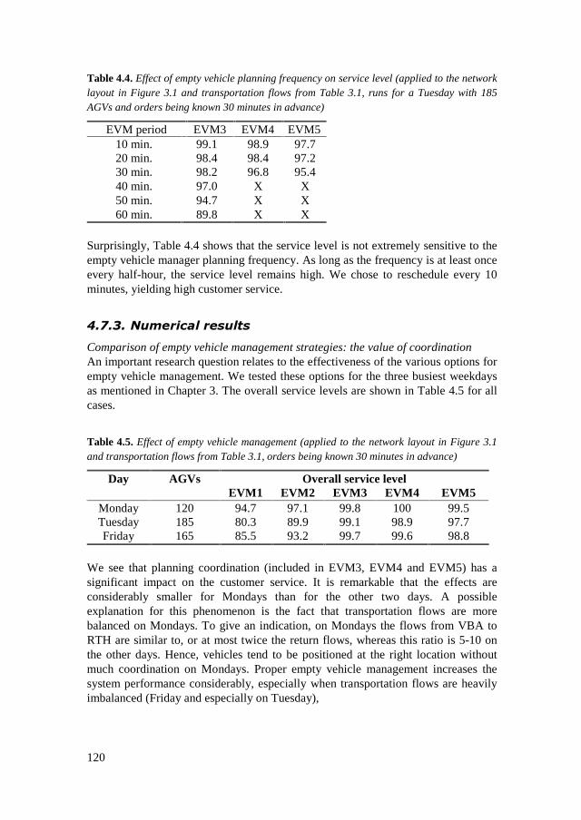
120

Table 4.4. Effect of empty vehicle planning frequency on service level (applied to the networklayout in Figure 3.1 and transportation flows from Table 3.1, runs for a Tuesday with 185AGVs and orders being known 30 minutes in advance)

EVM period EVM3 EVM4 EVM510 min. 99.1 98.9 97.720 min. 98.4 98.4 97.230 min. 98.2 96.8 95.440 min. 97.0 X X50 min. 94.7 X X60 min. 89.8 X X

Surprisingly, Table 4.4 shows that the service level is not extremely sensitive to theempty vehicle manager planning frequency. As long as the frequency is at least onceevery half-hour, the service level remains high. We chose to reschedule every 10minutes, yielding high customer service.

��6��

Comparison of empty vehicle management strategies: the value of coordinationAn important research question relates to the effectiveness of the various options forempty vehicle management. We tested these options for the three busiest weekdaysas mentioned in Chapter 3. The overall service levels are shown in Table 4.5 for allcases.

Table 4.5. Effect of empty vehicle management (applied to the network layout in Figure 3.1and transportation flows from Table 3.1, orders being known 30 minutes in advance)

Day AGVs Overall service levelEVM1 EVM2 EVM3 EVM4 EVM5

Monday 120 94.7 97.1 99.8 100 99.5Tuesday 185 80.3 89.9 99.1 98.9 97.7Friday 165 85.5 93.2 99.7 99.6 98.8

We see that planning coordination (included in EVM3, EVM4 and EVM5) has asignificant impact on the customer service. It is remarkable that the effects areconsiderably smaller for Mondays than for the other two days. A possibleexplanation for this phenomenon is the fact that transportation flows are morebalanced on Mondays. To give an indication, on Mondays the flows from VBA toRTH are similar to, or at most twice the return flows, whereas this ratio is 5-10 onthe other days. Hence, vehicles tend to be positioned at the right location withoutmuch coordination on Mondays. Proper empty vehicle management increases thesystem performance considerably, especially when transportation flows are heavilyimbalanced (Friday and especially on Tuesday),

121

For the cases mentioned in Table 4.5, EVM3 and EVM4 have more-or-less the sameoverall service level, while EVM5 shows slightly worse results. To ascertainwhether this is a general result, we constructed an additional artificial case. Thiscase was based on the same network, but with a different transportation pattern. Totest the empty vehicle managers under difficult conditions, we defined transportationpatterns with peak levels moving quickly from one route to the other. This meansthat to attain high customer service levels it is essential to anticipate heavilyfluctuating transportation demands. For this case, we found that EVM4 performssignificantly better than EVM3 (service level 98.5% versus 95%), while EVM5 alsoperforms rather well with a service level of 97.8%. In Figure 4.6, EVM5 has the bestthroughput time distribution, but there are several jobs that have a throughput timelonger than 2 hours. The throughput time distribution under EVM4 is alsosignificantly better than that of EVM3. We conclude that EVM4 is preferable in thesense that its performance is at least equal to that of EVM3, and under difficultconditions considerably better than that of EVM3. EVM4 also outperforms EVM5with regard to service level. Moreover, as stated in Section 4.7.2, we could runEVM4 with more parameter settings or priority rules to improve its performance.

0

10

20

30

40

50

60

70

80

90

100

0:00

0:10

0:20

0:30

0:40

0:50

1:00

1:10

1:20

1:30

1:40

1:50

2:00

2:10

2:20

2:30

throughput time

cum

ula

tive

per

cen

tag

e

EVM3

EVM4

EVM5

Figure 4.6. Throughput time distribution for EVM3, EVM4 and EVM5 in the case of fictitioustransportation flows with quickly moving peak levels between routes

For the three best empty vehicle managers, EVM3, EVM4 and EVM5, we comparedthe average empty travel distance per day. We found that EVM4 requires 3-10% lessempty travel than EVM3, and 15-30% less empty travel than EVM5, depending onthe day. In case of sufficient AGV capacity, EVM5 tends to send more empty AGVsto a terminal than is strictly necessary. Hence, EVM4 is also more efficient from anenvironmental point of view. Furthermore, empty travel reduction is relevant whenAGVs use batteries for energy provisioning, because the recharging frequency isreduced.

122

Impact of the information horizon: the value of informationAs mentioned before, pre-information about transportation jobs may facilitateplanning and improve the system performance. However, this requires additionalcommunication and hence more sophisticated organization and information systems.We analyze the effect of the period for which transportation jobs are known inadvance. As pre-information is only used for the empty vehicle manager options 2,3, 4 and 5, we omit option 1 (FCFS myopic). EVM2 (FCFS-look ahead) is identicalto EVM1 if pre-information is not available (horizon = 0). For EVM5 with aninformation horizon of 60 minutes we use a planning horizon (T) of 220 minutes,because more transportation jobs have to be planned. The main results are shown inTable 4.6.

Table 4.6. Effect of the period for which transportation jobs are known in advance.

Day AGVs Orders Overall service levelknown EVM2 EVM3 EVM4 EVM5

Monday 120 0 min. 94.7 99.4 99.0 98.130 min. 97.1 99.8 100 99.560 min. 90.3 99.9 100 99.3

Tuesday 185 0 min. 80.3 84.7 92.4 91.530 min. 89.9 99.1 98.9 97.760 min. 93.0 98.5 99.2 98.0

Friday 165 0 min. 85.5 90.0 94.8 93.030 min. 93.2 99.7 99.6 98.860 min. 95.6 99.9 99.6 99.1

We notice a similar phenomenon to that in the previous section, namely that theimpact of pre-information is highest if the transportation flows are heavilyimbalanced (Tuesday and Friday). Pre-information appears to have an even strongereffect on customer service than coordination. Of course, proper coordination isfacilitated by the availability of sufficient information. The marginal value ofadditional pre-information clearly decreases.

It is remarkable that for EVM2 the overall fill rate on Monday, with transportationjobs known 60 minutes in advance, is even considerably less than the rate when only30 minutes pre-information is available. This phenomenon can be explained asfollows. Vehicles are dispatched to the terminals FCFS once the transportation jobsare known. If transportation jobs are known 60 minutes in advance, AGVs arrive tooearly at the terminal and have to wait for a long time before they can be loaded,causing a significant capacity loss in a bottleneck resource (AGVs). In the OLS 30minutes to one hour of pre-information will be sufficient for practical purposes,because of the maximum travel times between the various locations in the network.

123

*�, ��9�:��

In this chapter, we developed several options for vehicle management in automatedtransportation networks. The various methods have been implemented and tested ina simulation environment for the OLS-case. We found that both information aboutfuture orders and planning coordination between terminals gives considerableadvantage in terms of customer service levels. In many cases a relatively simplemethod to balance empty vehicle flows in the system (EVM3), taking into accountsome future order information and communication with local (terminal) levels,already appears to provide considerable benefits. The advantage of EVM3 is therelatively low level of complexity and information exchange between local(terminal) and central (network) level.

A more advanced serial scheduling method (EVM4) can improve the performancefurther, especially in difficult cases when peak demand quickly moves from oneroute to another. In this case it is worthwhile to plan a sequence of orders in anintegrated way for a longer time horizon. Integrated planning also has the advantageof reducing empty travel. Moreover, the serial scheduling method offers a broadrange of possibilities for further refinements. In this respect, inclusion of finiteterminal capacities, both docking capacities and parking space, is an interestingsubject for further research (not in this thesis).

Another approach based on logistics queuing networks shows slightly worse resultsthan EVM3 and EVM4, but an advantage of the LQN approach of EVM5 is theflexibility. Due to the time-space decomposition, complicating constraints can beadded without a lot of extra computation time. Order acceptance could easily beimplemented, meaning that not all transportation jobs have to be transported.Nevertheless, we also encountered several disadvantages of the LQN algorithm. Thechoice of discrete time intervals may have some negative effects in the case of longtime intervals. The use of a linear approximation leads to an unstable objectivefunction, which does not converge to an optimal solution, as also noticed byCarvalho and Powell (1998). The LQN algorithm shows results that are within a fewpercent of the optimal solution, as was also claimed by Powell and Carvalho(1998a). However, we note that the same applies to the much simpler coordinatedlook-ahead rule (EVM3).

An advantage of the coordinated look-ahead rule (EVM3) is that because of thelocal control concept it can easily be extended to include complications such as two-way tracks. Two-way tracks are more difficult to incorporate in an integratedplanning approach, such as EVM4 or EVM5. For this reason, and because in thepractical cases with a positive information horizon the performance of EVM3 iscomparable to the performance of EVM4, we will use EVM3 in the remainder ofthis thesis.

125

�6�7 ��

)

�� :�� 9� 9�� E(

A�/A�? ��E�� '

)�� 89� :��

The realization of an underground transportation system, such as the OLS, requireshigh investments in both infrastructure and control systems. Dominant cost factorsare the total length of the tubes and their diameter. To ensure that the project isfeasible from an economic perspective, configurations are studied in whichterminals are connected by a single tube, allowing for traffic flows from one end at atime (cf. Figure 3.2). However, such options for the system layout may have asevere impact on the logistic performance, because AGVs are often forced to wait atthe tube entrances. Consequently, in order to guarantee acceptable throughput timesthere is a need for intelligent control of the driving direction.

In this chapter, we address a track/tube allowing for alternating traffic as a two-waytrack/tube. We describe the two-way track as a part of an underground automatedtransportation network, although the same setting applies to systems like bridges,tunnels or roadblocks caused by traffic accidents or road maintenance. As a startingpoint for our discussion we use Figure 5.1.

3 This chapter is partly based on Van der Heijden et al. (2001b).

126

Figure 5.1. Two-way track

The central part of Figure 5.1 is the two-way track, used for traffic in bothdirections. The AGVs arrive and depart on tracks that only allow one-way traffic.According to a control rule, AGVs arriving at the tube may either enter the tubeimmediately or queue until a signal is given that access to the single tube is allowed.Each control rule generates the system states, shown in Table 5.1, in cyclic order.

Table 5.1. Description of the system states

State Descriptiona AGVs from the right have to wait, but AGVs from the left are not yet

able to enter the track, because it still contains AGVs driving fromright to left; we use the term clearing the tube for this system state

b AGVs from the left can enter and AGVs from the right have to waitc AGVs from the left are stopped and AGVs from the right wait until the

tube is clearedd AGVs from the right can enter and AGVs from the left have to wait

The time spent in the states b and d is called the green time (since there is a green“traffic light” at the right and the left, respectively) and the time spent in states a andc is called the clearance time. The clearance time refers to the period with a redtraffic light at both ends, while vehicles still have to leave the tube. The cumulativetime spent in the four system states makes up the cycle time. The time spent in eachsystem state is variable and depends on the driving time on the two-way track, thearrival distributions at both sides and the control rule.

Left

Right

waiting driving clearing waiting

clearing waiting waiting driving

PL+PRCR PL PL+CLa dcb

Figure 5.2. System states under a periodic control rule

A main assumption in our modeling is that at each moment t it is known how manyvehicles are present on a track. Technologically, this can easily be accomplished, forexample by using induction wiring at both ends of the two-way track. Let us denotethe number of vehicles on the track driving from right to left and from left to right,as R(t) and L(t) respectively. The operation of the two-way track will always be suchthat the collision avoidance condition R(t)L(t)=0 holds true. Updating the counterR(t) is simple: in the case of an entrance at the right end of the two-way track we

127

have R(t+h)=R(t)+1, in the case of a departure at the left end we have R(t+h)=R(t)-1. For L(t) analogous updating rules with right and left interchanged hold true. Inthese rules h denotes a small time interval associated with electronic datatransmission. In addition, we assume that an end-of-clearance signal is available.The starts of the red light intervals can be considered as decision variables in theoperational control of the two-way track. As we will see shortly, there are severalways to set a decision rule for these decision variables: PL and PR.

Our study of the OLS raised the question of which rule should be used to controlaccess to the two-way track in order to minimize delay. Although central schedulingof all activities, including the two-way track, is theoretically possible for the OLSsystem, we chose to focus on local control rules fitting into the general frameworkas discussed in Chapter 2. This control rule for the isolated subsystem may take intoaccount information on the environment, such as expected AGV arrival times.

A straightforward well-known control rule in production management, which usesinformation on arrival times of vehicles, is First-Come First-Served (FCFS).However, this rule will only lead to a reasonable performance in the case of verylow traffic intensity and relatively short driving times along a two-way section (forexample crossroads). Therefore it is not applicable to the OLS, where a high trafficintensity and long tube driving times are envisaged (5-10 minutes). Another obviousoption is switching the driving direction periodically: PL and PR are constants. Thatis, the system spends a fixed time in both the system states a&b (PL) and in thestates c&d (PR), with P > T, where T is a measure of the driving time on the two-way track. So the green time depends on the preceding clearance time. Analternative simple control rule could be to fix the green time instead of the cycletime, i.e. spend a fixed time in state b and d. In this chapter we focus on the firstpossibility. An obvious drawback of these simple rules is that they do not useinformation on AGV arrivals and queues at both two-way track entrances. Hence, itis possible that AGVs have to wait at one entrance, while the two-way track is freeand no AGVs are present or approaching the other entrance. In particular when thetraffic intensities at both sides of the two-way track are different and/or fluctuate intime, a simple periodic control rule may lead to excessive waiting times. Therefore,we also developed adaptive control rules with increasing complexity andinformation usage. Information on future arrivals at the two-way track can beobtained, for example from induction wiring at a certain distance in front of theentrances of the two-way track. One can install counters for the numbers in thequeue at both ends of the two-way track. We focus on control rules that are suitablefor on-line control: they have to be efficient in terms of computation time. Thepotential of the new control rules is demonstrated by an extensive simulation studybased on independent Poisson arrivals of AGVs, as is plausible in an open system.We will also discuss the implications of embedding the two-way track in the OLS.More specifically, we will consider the effects of the convoys created at a two-waytrack on both terminal operations and on other two-way tracks in the system.

128

This chapter is structured as follows. In the next section we give an overview of theliterature, in which we relate the system studied to similar traffic, queuing andproduction systems. In Section 5.3, our model is defined in more detail. In Section5.4 we describe the periodic control rule, followed by the adaptive control rules inSection 5.5. The design of the simulation study is described in Section 5.6. InSection 5.7 we present the results of a simulation study of an isolated two-way track,while we focus on the implications of a two-way track in a closed system in Section5.8. Finally, in Section 5.9, we summarize the main conclusions.

)�� : �� 9��;:�A

The problem of controlling a two-way track appears to be at the intersection of anumber of research fields. While the link with the traffic literature, as described inSection 5.2.1, is intrinsically clear, other research is also relevant. In addition tothose mentioned in the traffic literature, we can find similar models in the queuingliterature, as described in Section 5.2.2. Furthermore, one can formulate the problemas a machine-scheduling problem, in which a planner has to decide when the nextbatch of products (product 1 is an AGV from the right, product 2 is an AGV fromthe left) should be processed (Section 5.2.3). Below we relate the two-way trackcontrol problem to these research fields.

5�� 3 ��

Linking two-way track control to what is mentioned in the dynamic traffic controlliterature seems natural as the system is intended to be an integral part of trafficsystems. Haight (1963) generalizes the problem of controlling two-way tracks andsimilar systems as the control of a road section that allows one-way traffic only.Given the arrival distributions and the allowed driving directions, either left-right orright-left, formulas are derived which specify queuing behavior. Two-way trackcontrol is also related to junction control supported by traffic signs. In the early daystraffic signals were usually scheduled according to a pre-determined scheme (cf.Bell, 1992). Such a scheme allowed traffic to be handled following a fixedsequence. A periodic control rule is a good example of such a scheme. Mung, Poonand Lam (1996) elaborated on Haight’s model and derive distributions of queuelengths at fixed time traffic signals. Heidemann (1994) derives analytical results onstatistical distributions of queue lengths and delays at traffic signals, given Poissonarrivals and a fixed-time control. The results are compared with severalapproximations (Webster, 1958; Miller, 1968). Hu et al. (1997) extend Heidemann’smodel to the multi-lane case, where multiple vehicles may enter the trafficintersection simultaneously. Nowadays, traffic signals are usually controlled byadaptive rules, which take the actual traffic situation into account. Usually trafficcontrol at intersections is vehicle dependent: the arrival of one vehicle can switch thetraffic light to green if there is no other demand for the resource. Increasingly, these

129

control rules become traffic dependent. A common objective is to minimize theaverage loss times, i.e. minimizing average waiting times. For example, Robertsonand Bretherton (1974) describe an optimal control policy for an intersection for anyknown sequence of vehicle arrivals. They compare the optimum policy with a fixedtime control policy and responsive control policies, a “saturation flow” and “no-flow” policy. The responsive control policies cannot be used for a two-way trackdue to the long clearance time of the two-way track.

In the traffic literature, it is usually assumed that the effective green period and theeffective red period are constant and known. If this assumption is valid, we couldsimply use the exact method proposed by Heidemann (1994). As appears from ourproblem statement in the introduction, this is not the case in our situation. Theclearance time is a random variable and depends on the last moment at which avehicle enters the two-way track before the traffic light is switched to red. The useof fixed effective green times would be reasonable if the passing time of the lanewas negligible. It is also a reasonable assumption if the system runs close tomaximum capacity, so that the vehicle queue has usually not yet disappeared or hasjust disappeared when the traffic light is switched to red. In the latter case, theclearance time equals the deterministic driving time along the shared lane, so theeffective green time is fixed too. Some preliminary numerical experiments applyingHeidemann’s (1994) method to our modified model, revealed that in this way thewaiting time can be overestimated by 5-10% over the entire parameter range. This isa result of the fact that the clearance time is less than or equal to the driving timealong the lane, causing a longer effective green time. Therefore, we conclude that itis useful to construct a dedicated method to calculate mean waiting times.

An essential difference between an automated transportation system and trafficsystems, as discussed here, is that the behavior of AGVs can be directly influenced.Human drivers feel a need for a “fair” handling of traffic and therefore restrictionsare set to maximum cycle times, which is roughly the maximum waiting time for acar. Moreover, quite precise information is available on expected arrival times ofAGVs at the two-way track entrance, because the driving behavior of AGVs is farmore predictable than that of passenger cars.

5�� <��

As well as in the traffic literature, we can also find similar models in the queuingliterature. To be specific, our model has similarities with polling systems (cf.Takagi, 1990), in which a single server handles two queues and switches betweenthem according to some control rule. For our model, the service time should bedeterministic and equal to the minimum distance between successive vehicles,expressed in time. Furthermore, the server attends both queues for a fixed period oftime. This aspect is not common in polling models, but can be found in STDM(Service Time Division Multiplexing, cf. Kleinrock, 1976). However, STDMmodels do not include switchover times. In our setting, the clearance time could be

130

modeled as a random set-up time, depending on the timing of the last service at theother queue. This aspect is not common in queuing systems.

Related to polling systems are queuing models with vacations (Doshi, 1990; Takagi,1991). The server leaves the queue regularly to perform other tasks. In our case, thevacation period can be modeled as some random variable that depends on theswitching interval P, the driving time along the lane, T, and the vehicle arrivalprocess. We would still need a decomposition between the queues at both sides ofthe shared lane, whereas these queuing processes are actually interrelated. InDoshi’s (1990) classification, our model is closest to the category withasynchronous vacations and general vacation rules. We did not find a model similarto ours in the literature on vacation queues.

5�� : ��

In the machine scheduling literature, problems rather similar to the two-way trackproblem are studied. Several batching strategies are developed within the context ofdeterministic scheduling. For overviews see e.g. Uzsoy et al. (1992, 1994), Websterand Baker (1995), and Potts (2000). An alternative approach is taken by anothergroup of authors (Glassey and Weng, 1991; Fowler et al., 1992; Weng andLeachman, 1993; Van der Zee et al., 1997), who study the batching problem in adynamic context, where jobs have to be scheduled realtime given the availability ofinformation on some or all near future arrivals. Many of these studies focus on thecontrol of oven systems found in semiconductor manufacturing and aircraft industry.Similarities between the two-way track system and such systems can be found in thefact that goods (AGVs) have to be “batched”, with the processing time of a batchequal to the driving time on the two-way track, and the dynamic nature of theproblem. An essential difference can be found in the fact that for the two-way tracksystem there is no fixed processing time. While for oven systems processing timesare related to static product and process characteristics, the processing time of aconvoy on a two-way track depends on the time between the first and the last AGVin a convoy. Furthermore, oven systems set restrictions on the number of products ina batch, but there is no a priori limit on the number of AGVs in a convoy.

Summarizing, the most important differences compared to the literature are:(a) Significant throughput time on the two-way track (several minutes).(b) The clearance time is variable, depending on the time at which the last AGV

entered the two-way track.(c) No maximum batch size.

131

)�' �� 9��7 �

5�� 7��

For reasons of clarity of understanding, and to keep the formulas simple, we makethe following simplifying assumptions for the system characteristics:1) All AGVs are identical.2) When driving, the AGVs travel at a constant speed.3) Queuing AGVs accelerate instantaneously to their normal speed, when

activated, and AGVs can stop instantaneously when arriving at a queue.4) AGVs waiting in queue enter the shared lane with a fixed minimum succession

time (δ), that remains constant while driving on the two-way track.5) The length of an AGV is negligible (can be included in δ).

In practice, the succession time between vehicles will be strictly positive. Anobvious reason is the length of a vehicle; two vehicles cannot enter a single lanesimultaneously. Also, safety margins can be included to take into account a finitedeceleration. These safety margins should be set such, that the collision probabilityis negligible. We use the brick wall principle (cf. Chapter 3, Section 3.3.3). Thisprinciple states that when travelling with the minimum succession interval a vehicleshould be able to stop in time if the preceding vehicle comes to a dead stop. Safetymargins for finite acceleration can be incorporated in the minimum distance. Theeffect of stochasticity in the AGV speed (for example load dependent) can be putinto a safety margin by working with a slightly lower constant speed than themaximum speed. In the OLS-case, for example, the maximum speed of an AGV is 7m/s (cf. Chapter 3), but we use an operational speed of 6 m/s. Note that we do notmake an explicit assumption about the arrival processes as far as lot-size isconcerned. Both single and batch arrivals are considered. In the remainder of thissection we characterize the rules for real-time two-way track control in terms ofinformation usage and decision structure. For a detailed description of the controlrules we refer to Sections 5.4 and 5.5.

5�� +� ��= ��

If information is available on all AGV arrivals it is possible to construct an optimalschedule (cf. the concept of deterministic machine scheduling). In a dynamicsituation however, information changes as a result of additional AGV arrivals orbetter forecasts of arrival times. We consider the case in which arrival information isknown for arrivals up to t0+H, with t0 a decision moment and H the informationhorizon. Arrivals after time t0+H are assumed to be unknown. Hence, as timeproceeds, new information may become available. This leads to a rolling horizonapproach. In consequence, rescheduling is necessary. This implies that therescheduling frequency appears as an additional parameter.

132

We consider three situations as far as information on AGV arrivals is concerned:(a) No information on AGV queues and arrivals.(b) Only local information on queue lengths at the tube entrances is available

(H=0).(c) Prior information, i.e. both on current queue lengths and on future arrivals

within a certain information horizon H > 0 is available.

Now we can classify the control rules according to the available information anddecision options, see Table 5.2.

Table 5.2. Classification of the control rules

noinformation

localinformation

priorinformation

one change adaptive localcontrol

adaptive look-ahead control

multiple changes

periodiccontrol

dynamic programming

If no information on the AGVs waiting or arriving is available, a periodic controlrule is the only realistic option. In that case, the only issue is to determine the fixedtime interval P, as introduced in the previous section. The interval chosen is basedon off-line optimization, considering the historical and/or expected traffic flows, asin off-line junction control (Bell, 1992). The periodic control rule will be discussedin Section 5.4. The advantage of a periodic control rule lies in its simplicity; itrequires no information on system status.

In the other cases a decision policy has to be constructed. A policy has to define theset of decision moments t0, and for each decision moment the allowed decisions.Policies open to the controller are either to take a single decision on the timing ofthe next direction change, or to make a schedule of multiple direction changeswithin the information horizon H, i.e. all known AGV arrivals (jobs) are included inthe schedule. We restrict the decision moments to the following list of discreteevents:(I) the end of state a, where the two-way track is cleared for traffic from the

left;(II) the arrival of a new AGV at the left or the right end of the two-way track in

state b, with a green traffic light at the left entrance;(III) the end of state c, where the two-way track is cleared for traffic from the

right;(IV) the arrival of a new AGV at the left or the right end of the two-way track in

state d, with a green traffic light at the right entrance.

At each decision moment the allowed decisions are: “let the green traffic lightremain green until the next decision moment” or “put the green light on red so that achange of direction is enforced immediately after this decision moment”. Sometimes

133

the choice of a next decision moment is modified in the sense that it is the first eventof type (I-IV) after a lower bound in time after the previous decision moment. In thisway, one can enforce that a certain batch of vehicles enters the tube. Usually, it onlymakes sense to change the two-way track direction directly after an AGV hasentered the two-way track. The additional decision moments are sketched above.Too frequent rescheduling may result in excessive computation times.

Information on the AGVs in queues and/or information on arrivals can be used toimprove system performance by developing control rules that use this information.These are adaptive control rules (see Section 5.5). The construction of such anadaptive control rule implies finding an optimization criterion to determine thedirection changes. When only local information on queue lengths is available, andthe direction is changed to right-left, then obviously the whole queue at the rightfirst passes the tube. It can easily be shown that any other option, for exampleprocessing the queue at the right in two separate batches, is inferior in terms of totalwaiting time for the vehicles in queue because of the additional clearance time incase of an additional direction change. For this reason, a dynamic programmingapproach that considers multiple changeovers naturally leads to batch processing;the entire queue present at the decision moment enters the two-way track.

We consider two decision options based on information on future arrivals (see Table5.2). First, we develop a look-ahead criterion for determining the next directionchange (Section 5.5.2). Second, a dynamic programming rule is introduced (Section5.5.3), which computes an optimal sequence of direction changes. In a rollinghorizon approach only the first change in this sequence is used, but the computationstake future direction changes into account.

The decision about changing the direction should be based on some optimizationcriterion. As our focus in the OLS is to minimize average order throughput times,we chose minimum average waiting time at the two-way track as criterion. Thewaiting time is defined as the time from the arrival of an AGV at the entrance of thetwo-way track until it enters the two-way track. The basic ideas presented in thischapter can also be applied to other criteria, such as minimum lateness.

)�* ��:�8:��

5�� .��

In Section 5.2 we have seen that similar models to the one under consideration havebeen analyzed, but also that as far as we know the combination of a fixed (periodic)service schedule, random clearance times and correlated queuing processes is new.

134

For the periodic control rule we proceed from Figure 5.2 in Section 5.1. The foursystem states constitute a cycle. The time spent in system state b (d) is called theeffective green time from the left (right). We refer to the time spent in system state a(c) as the clearance time, denoted by CL (CR). Obviously, the clearance time isvariable and depends on the moment the last vehicle enters the lane before the trafficlight is switched to red. In all cases, the clearance time varies between 0 and thedriving time on the two-way track, denoted by T.

We define a periodic control rule such that the time spent in system states a plus b isconstant and equal to PL, see Figure 5.2. Analogously, the time spent in systemstates c and d is constant and equal to PR. Hence, the total cycle length equals PR+PL

and the effective green time from the right (left) equals PR-CL (PL-CR). The keyproblem is to determine PL and PR such, that vehicle waiting times are minimized.To this end, we need to calculate the mean waiting times for vehicles arriving atboth sides of the two-way track as a function of the control parameters PL and PR. Ifthe vehicle arrival processes at both sides of the two-way track are the same, it isreasonable to take PL=PR=P. We refer to this situation as the symmetric case. In thissection, we address the symmetric and the asymmetric case (PL≠PR).

AssumptionsWe focus on the computation of the mean waiting time at a periodically switchedtwo-way track as described in the introduction. If we have an expression for themean waiting time, we can use a standard numerical search procedure to find theoptimal value of the switching period P in the symmetric case; we have to find bothPR and PL in the asymmetric case.

We make an additional assumption to the ones already mentioned in Section 5.3.1.AGVs arrive one-by-one according to a Poisson process, not necessarily identical atboth sides of the two-way track. With respect to this assumption, we note thatPoisson arrivals are theoretically conflicting with the assumption on minimumsuccession times, as Poisson arrivals allow succession times that are almost zero.Many papers use the assumption of Poisson arrivals for convenience. This does notseem to be very harmful from a practical point of few if the probability that avehicle arrives within the minimum succession time is negligible, which is satisfiedin many practical cases. Although we base our derivations on Poisson arrivals, wewill discuss the generalization to compound Poisson arrivals in Section 5.4.7.

Model input:T = the driving time of a single vehicle to pass the two-way trackA(t) = the number of vehicles arriving at one side of the two-way track during

an arbitrary time period with length t, a random variableλ = the vehicle arrival rate at one side of the two-way trackδ = the minimum time between two successive vehicles entering the two-way

track

135

Model output:C = clearance time of the two-way track, a random variableW = vehicle waiting time, a random variable

Control parameter:P = Fixed period for traffic from one side to enter the two-way track; the cycle

length equals 2P (symmetric case)

As stated before, we may give the parameters P and λ and the random variables W,C and A() a subscript R or L, denoting the respective characteristics of the right andleft side of the two-way track. In an asymmetric case with different arrival rates λL

and λR, the length of the green period at the left (right) end of the two-way trackequals PL-CR (PR-CL). Analogously, the length of the red period at the left (right) endof the two-way track equals PR+CR (PL+CL). As we consider identical vehicles, thedriving time on the two-way track, T, as well as the minimum mutual distancebetween vehicles, δ, does not depend on the driving direction. Therefore, thesubscripts R and L are omitted for these parameters. From a theoretical point ofview, it is straightforward to include non-identical values of T and δ.

As we explained in Section 5.2, this problem is related to other models encounteredin traffic management literature and has also similarities with some queuing models(polling systems, M/D/1 vacation queue). However, we did not encounter thisparticular model in the literature. Therefore, we developed approximate methods tocalculate the mean waiting time at a two-way track for several variants. We startedwith the analysis of a simple case, namely a symmetric model where the successiontime, i.e. the minimum time between successive vehicles entering the two-way track,is zero. For this special case, we can develop an exact method to calculate the meanwaiting time as well as a simple approximation. It is more realistic that minimumsuccession times are strictly positive, taking into account the vehicle length and aminimum safety distance to avoid collisions. For this more general case, we are onlyable to derive approximate expressions. Therefore, we validated our approximationmethod by comparing the outcomes to simulation results. We subsequentlyaddressed the symmetric and asymmetric cases. In all our models, we assumePoisson arrivals at both ends of the two-way track. However, extension to moregeneral arrival processes is possible, and we will briefly discuss how to accomplishthat.

The remainder of this section is structured as follows. First, we give the notation tobe used throughout this section. The simple case with zero minimum vehiclesuccession time is discussed in Section 5.4.3, and some numerical results are shownin Section 5.4.4. The analysis for strictly positive minimum succession times isgiven in Section 5.4.5, for both the symmetric and the asymmetric cases. Thecorresponding numerical results are shown in Section 5.4.6. In Section 5.4.7 wedescribe how our method can be extended to compound Poisson arrivals.

136

5�� ,� ��#��

In a periodic control rule, the setting of the time interval P is restricted by the needto clear the two-way track every time the driving direction is changed. Inconsequence, the time interval P should exceed the maximum clearance time: thedriving time T. It is straightforward to define necessary and sufficient conditions forsystem stability. We present these conditions for the symmetric as well as theasymmetric case. For the symmetric case, we can derive the stability condition byintuition. First, we note that the effective green period equals P-T in the worst case,because the clearance time C equals the driving time T if there is heavy traffic.Second, we observe that the maximum number of vehicles that can be processedduring the effective green period should exceed the total number of arrivals in acycle. Hence we find that ( ) / 2P T Pδ λ− > or, equivalently,

1 2

TP

λδ>

− (1)

This condition was formally derived by Meissl (1963) and can easily be extended tothe asymmetric case. Then it is necessary that, at both sides of the two-way track,the expected number of arrivals in a cycle with length PL+PR can be served in theexpected green time. This expected green time equals PL-T at the left and PR-T at theright side of the two-way track. Therefore, the following two stability conditionsapply:

1( ) ( ) (1 )L L R L L L L RP P P T P T Pλ λ δ λ δ

δ+ < − ⇔ − > + (2)

1( ) ( ) (1 )R L R R R R R LP P P T P T Pλ λ δ λ δ

δ+ < − ⇔ − > + (3)

These two equations define the feasible area in 2R for which the system is stable.As can be expected, conditions (2) and (3) reduce to the stability condition for thesymmetric case (1) if L Rλ λ λ= = .

5�� > ��&δ?@*

In this section, we derive expressions for the mean waiting time E[W] for thesymmetric case with minimum succession time δ=0. For ease of notation, we omitthe subscripts R and L. First, we note that, conditional on the clearance time C, thewaiting probability equals (P+C)/2P. Second, we exploit the fact that theexponential inter-arrival distribution corresponding to Poisson arrivals has the well-known memory-less property. So if a vehicle has to wait, the mean waiting timeequals (P+C)/2. This gives:

137

[ ] [ ] [ ] 22 2( )|

4 4 2 4 4 2 4

E CE CP C P C C PE W C E W

P P P

+ = = + + ⇒ = + + (4)

Therefore in order to compute E[W] it is sufficient to derive an expression for thefirst two moments of the clearing time C. We show how we can compute theprobability distribution of the clearance time C exactly, so we can compute the firsttwo moments of C exactly as well.

When P>2T, the effective green time P-C certainly exceeds T, because C≤T. In thatcase, the clearance time is fully determined by the last arrival before the drivingdirection is changed. Then we find that

( )

Pr{ 0} Pr{no arrivals in [0, ]}

Pr{0 } Pr( 1 arrivals in [0, ]} 1

T

T t

C T e

t C T T t e

λ

λ

−

− −

= = =< < < = ≥ − = −

Note that in this case the distribution is independent of P.

When T<P≤2T, the situation is more difficult. Nevertheless, we can exploit the factthat C has to satisfy a fundamental relationship. Let IR and IL denote indicatorswhether at the start of a green traffic light interval at the right and left end of thetwo-way track, respectively, vehicles are present (indicator=1) or not (indicator=0).Let Y be the length of the interval beginning when the traffic light becomes greenand ending when the last vehicle during that green traffic period enters the two-waytrack. It is clear that

1 0

0L R L R

L

C C Y T P if I and C Y T P

C else

= + + − = + + − >=

(5)

Noting that ( )Pr{ 0 } PL RI C e λ ττ − += = = , we find that

( )

( ) ( ) ( ) 2

Pr{0 } 1 max(0, )

Pr{0 } (1 ) (1 ) 1

T tL R

P P P PL R

t C T C e if t T

t C T C e e e e if T t

λ

λ τ λ τ λ τ λ

τ τ

τ τ

− −

− + − − − + −

< < < = = − − ∆ < <

< < < = = − + − = − > > + ∆

Due to the symmetry in the arrival processes, CR and CL are identically distributed.Denote their probability density as f(t) and let us introduce the shorthand notation

0

( ) Pr{0 } Pr{0 } ( )T

L Rdef

G t t C T t C T C f dτ τ τ= < < < = < < < =∫Note that f(t) has a point mass at t = 0; the integral should be interpreted as includingthis effect. It is crucial that G(t) satisfies a fundamental difference equation. Using

138

the relation with the conditional probabilities given above, we find after integrationwith respect to τ:

( ) 2

min( , ) min( , )

( ) ( ) 2

( ) (1 )(1 ( ) ) (1 ) ( )

1 ( ) ( )

T TT t P

t T t T

T t T t P

G t e f d e f d

e e e G t

λ λ

λ λ λ

τ τ τ τ− − −

+∆ +∆

− − − − −

= − − + − =

− + − + ∆

∫ ∫ (6)

where ∆ = P-T. Of course, G(t+∆) has to be interpreted as 0 if t+∆ > T. Thestructure of this equation is such that it can easily be solved recursively:first [ , ], next [ 2 , ], etc.t T T t T T∈ − ∆ ∈ − ∆ − ∆ This leads us to

( )

( ) ( ) ( ) 2

1( ) ( ) ( ) 2

1 0

1 [ , ]

( ) 1 (1 )( ) [ 2 , ]

(1 ) (1 ) ( ) [ ( 1) , ]

T t

T t T t T t P

knT t T t k T t l P

k l

e t T T

G t e e e e t T T

e e e e t T n T n

λ

λ λ λ λ

λ λ λ λ

− −

− − − − −∆ − − −

−− − − − − ∆ − − − ∆ −

= =

− ∈ − ∆

= − + − − ∈ − ∆ − ∆

− + − − ∈ − + ∆ − ∆

∑ ∏

Equation (6) can easily be proved using induction. The analysis leads us to sums ofexponential functions for G(t) and f(t) for t > 0. This computation is completed bynoticing that the clearance distribution has a point mass at t = 0, such that its totalmass equals 1. In this way, all moments of C can be computed. Note that in generalthe probability of no arrivals in a cycle will be negligible, so 2 0Pe λ− ≈ . If wesubstitute this in the equations above, we can derive a simple and accurateapproximation for the clearance time distribution:

12

( 1) ( )( ) 1 [ ( 1) , ]

n T t nG t e for t T n T n

λ− + − − ∆≈ − ∈ − + ∆ − ∆ (7)

It is easy to derive the first two moments of the clearance time from this expression.Defining the integer N as T/∆, the largest number smaller than or equal to T/∆, wefind:

1 12 2

1( 1) ( ) ( 1) ( )

00 ( 1)

[ ]T N T nN

N T t N n T t n

n T n

E C T e dt e dtλ λ

− ∆ − ∆−− + − − ∆ − + − − ∆

= − + ∆

≈ − −∑∫ ∫

After some manipulations, this equation can be reduced to

1 1 1 12 2 2 2

( 1)( ) ( 1)( 2) ( 1) ( 1)1

1

1[ ]

( 1) ( 1)

N T N N N N N n nN

n

e e e eE C T

N N n n

λ λ λ λ

λ λ λ λ

− + − ∆ − + + ∆ − + ∆ − + ∆−

=

−≈ − − + ++ +∑ (8)

139

Analogously, we can derive for the second moment

( )

( )

1 12 2

1 12 2

( 1) ( 1)( )

2 22 2

( 1) ( 1)( 2)1

2 20

[1 ( 1)( ) ][ ] 2

( 1)

[1 ( 1)( ) ] [1 ( 1)( ( 1) ) ] 2

( 1)

N N N T N

n n n nN

n

N T N e eE C T

N

n T n e n T n e

n

λ λ

λ λ

λ

λ

λ λ

λ

− + ∆ − + − ∆

− + ∆ − + + ∆−

=

− + − ∆ −≈ +

+

− + − ∆ − − + − + ∆+

+∑

(9)

The calculation of the approximate values of E[C] and E[C2] from the expressionsabove is straightforward. The most convenient way to compute the mean waitingtime is to combine the equations (4), (8) and (9).

5�� δ�?�@

We use the equations obtained in the previous section for a numerical analysiswhich gives some insight into the optimal value of P. We choose T = 7 minutes forall our numerical experiments, this being a representative value for the OLS-case.Figure 5.3 shows the average waiting time as a function of the switching period Pfor various vehicle arrival rates λ (all time units in minutes).

6.6

6.7

6.8

6.9

7

7.1

7.2

7 7.5 8 8.5 9 9.5 10

P

E[W

]

lambda=2

lambda=5

lambda=10

lambda=20

Figure 5.3. Expected waiting times for periodic control, T=7 minutes

We can see that around the optimum the average waiting time only varies by a fewpercent. As can be expected, the average waiting time increases with the trafficintensity. Another observation is that the optimum switching period P decreases(and so does the effective green time) as traffic intensity increases. This is due to theassumption that a batch of vehicles can enter the two-way track in negligible time,irrespective of the batch size. If the driving distance between vehicles is positive (δ> 0), we expect an opposite effect, which will be confirmed in Section 5.4.6.Therefore, the equations as derived in the previous section are only useful if theminimum driving distance between vehicles is negligible indeed, for example, if a

140

train of vehicles can be constructed by magnetic coupling while vehicles are waitingin front of the entrance.

5��5� > �� #��&δ�A�@*

When mutual distances between vehicles are significant, we construct anapproximation that is closely related to the case with δ = 0. We start from thefollowing assumption:The probability that a vehicle encounters more than two traffic light switches duringits waiting time is negligible.

Based on this assumption, we can use the following decomposition of the meanwaiting time:

2

0

[ ]* [ ( )] [ * | ]ss

E W E A cycle E K W S s=

= =∑ (10)

whereE[W] = waiting time per vehicle.S = the number of traffic light switches during the AGV waiting

time.Ks = the number of vehicles in a cycle for which S=s and W>0, note

that Ks and W|S=s are not independent.E[Ks*W|S=s] = the total expected waiting time of all vehicles which encounter

S=sand where [ ( )] ( )R LE A cycle P Pλ= + in case of Poisson arrivals. Note that the

assumption above is formalized as Pr{S ≥ 3} = 0.

In this section we use the following, additional notation:M = the number of AGVs remaining in queue when the traffic light is

switched to redN = the number of AGVs in queue when the traffic light is switched to greenZ(n) = the time until a queue with length n vanishes, if the traffic light is green

and not switched to red; AGVs enter the tube at rate 1/δ and additionalAGVs arrive according to the process A(t), being a Poisson process withrate λ

x = the smallest integer larger than or equal to x

x+ = max{x,0}

For the asymmetric case, the parameter S and the random variables Ks, M, N andZ(n) have a subscript R or L, referring to the side of the two-way track (right or left).We derive all equations for the asymmetric case and state which simplificationsapply to the symmetric case. The equations will be stated in terms of the waiting

141

time at the left side. Obviously, similar expressions apply for the right side of thetwo-way track, where the subscripts L and R are interchanged in all expressions.

We proceed as follows. First we derive expressions for the three components ofequation (10), [ * | ]sE K W S s= for s=0, 1 and 2. We will see that these expressions

contain the first and/or second moment of the random variables M, N, Z(n) and C.Therefore, we derive expressions for these components. At the end of this sectionwe summarize our algorithm.

Basic expression for the waiting time componentsWe first classify all vehicles arriving at the left side of the two-way track in a cyclewith length PL+PR as a member of one of the sets having SL=0, SL=1 or SL=2. In thisway, we obtain approximate expressions for the numbers KL,s (s=0,1,2).

For vehicles arriving at the left side of the two-way track, a cycle with lengthPL+PR, consists of an effective red period of length PR+CR and a subsequenteffective green period of length PL-CR. The mean number of vehicles arriving in thiscycle equals λL (PL+PR). By definition the number of vehicles in queue at the startof the cycle (start of the red period) equals ML. All vehicles arriving in a greenperiod have an even value of SL (0 or 2, ignoring higher order terms) and all vehiclesarriving in a red period have an odd value of SL (1, ignoring higher order terms). Thelatter implies that

,1 ( )L L R RK A P C≈ + (11)

The vehicles arriving during the green period that cannot be handled in the samegreen period have SL=2. This number equals the number of vehicles in queue at theend of the first green period (ML), excluding the vehicles that were already in queueat the end of the preceding red period and that could not be served in the first greenperiod. Based on our assumption, we can ignore the latter number, as SL=3 for thosevehicles. Therefore, we find

,2L LK M≈ (12)

The number of vehicles that arrives in a green period and can be handled in the samegreen period equals 1

,0 * { ( ), }L L L R LK Min Z N P C Nδ −= − − . This stochastic variable

is difficult to handle because it requires the complete distribution of ZL(NL).However, if the system is not close to its stability boundaryPr{ ( ) } 0L L R RZ N P C> − ≈ . Therefore, we use the following approximation for KL,0:

,0

( )L LL L

Z NK N

δ≈ − (13)

142

We use (11)-(13) to derive expressions for the waiting time components

,[ * | ]L s L LE K W S s= (s=0, 1, 2).

SL=1.In this case the average waiting time consists of the following two components:• the waiting time during the red period; on average 1

2 ( )R RP C+ .

• the time until the vehicle can enter the two-way track after the light hasswitched to red. The number of vehicles waiting at the start of a green periodequals

,1( )L LM K+ ; as they enter the two-way track at rate δ, the average

additional delay is 1,12 ( 1)L LM Kδ δ+ − . This formula covers the fact that all

KL,1 vehicles have to wait until the first ML vehicles enter the two-way track,and the fact that the nth vehicle enters the two-way track at time (n-1)δ after thetraffic light turns to green.

So 1,1 ,1 ,1 ,12* ( | 1) ( 1)L L L L R R L L LE K W S E K P C K K Mδ δ = = + + − + .

Noting that ML and KL,1 are independent, but KL,1 and CR are not, we can write thisequation as

{ } 21 1 1 1,1 ,1 ,1 ,12 2 2 2* ( | 1) [ ] [ ] [ ] [ ]L L L L R L R L LE K W S E K C E K P E M E Kδ δ δ = = + + − + (14)

Note that CR refers to the clearance time as part of the red period after the queuewith length ML has been created, so K1 and ML are mutually independent. Toevaluate (14), we need:

1[ ] [ ( [ ])] ( [ ])L R R L R RE K E A P E C P E Cλ≈ + = + (15)2

1[ ] [ ( )] ( [ ]) [ ]L R R L R R L RVar K Var A P C P E C Var Cλ λ≈ + = + + (16)

[ ] 21[ ] ( ) [ ( )] [ ] [ ]R R L R R L R R R L R R L RE K C E C A P C E C P C P E C E Cλ λ λ≈ + = + = + (17)

Here we used the fact that for any correlated pair of random variables X and Y thewell-known conditioning formulas apply:

{ }[ ] [ | ]E X E E X Y=

{ } { }[ ] [ | ] [ | ]Var X E Var X Y Var E X Y= + .

SL=2.The waiting time of the KL,2 ≈ ML vehicles remaining at the end of a green periodconsists of the following components:• the length of the next red period PR+CR.

143

• the average time until the vehicles enter the lane when the light is switched togreen, 1

2 ( 1)LM δ− .

• the average time that the vehicles have been waiting when the light is switchedto red, 1

2 /L LM λ .

Analogously to the derivation of (14), and using the fact that ML and CR areindependent, we can state that:

2 11 1,2 2 2* ( | 2) [ ]( [ ] ) [ ]( )L L L L R R L LE K W S E M P E C E Mδ λ δ− = ≈ + − + + (18)

SL=0.KL,0 vehicles arrive during a green period when the queue of vehicles that is presentat the start of the green period (with length NL) has not yet entered the tube. Asnoted before, this period has length ZL(NL). The corresponding waiting time consistsof the following components:• the average time until the vehicles can enter the lane, calculated from the

moment the light is switched to green, 1,02 ( 1)L LN Kδ δ+ − .

• minus the average time that the vehicles arrive after the traffic light is switchedto green; using that the vehicles arrive during the period ZL(NL), and usingequation (13), we find that this correction term equals1 1

,02 2) )( (L LL LZ KN N δ= + .

So after some algebraic procedures we find:

{ }1,0 ,0 ,02[ * ( | 0)] [ ] [ ]L L L L L LE K W S E K N E K δ= ≈ − (19)

where

0

[ ( )][ ] [ ]L L

L

E Z NE K E N

δ≈ − (20)

and

{ } 20

1[ ] ( ) [ ]L L L L LE K N E N Z N E N

δ≈ − (21)

The auxiliary random variables M, N, Z(N) and CEquations (14)-(21) together with (10) give an approximation of the mean waitingtime, but before we can solve these equations we need the following characteristicsof the random variables M, N, Z(N) and C:• the first two moments of the number of vehicles remaining in queue at the end

of a green period, ML, for equations (14) and (18);• the first two moments of the number of vehicles in queue at the start of a green

period, NL, for the equations (20) and (21);• the first two moments of the clearance time, CR, for the equations (15)-(17);• the expectation of the time taken by the queue to enter the tube from the start of

a green period, ZL(NL), for equation (20);• the expectation of the product of ZL(NL) and NL for equation (21).

144

Below we derive formulas for these characteristics.

The queue lengths ML and NL.First, we observe that the following relations exist between M, N and C:

( )L L L R RN M A P C= + + (22)

( ) ( ) / ( ) ( ) /L L L L R L R L L L R L RM N A P C P C M A P P P Cδ δ+ +

= + − − − = + + − − (23)

where the random variables ML at the right and left hand side refer to twosubsequent cycles.

Equation (23) can be solved analytically to obtain the distribution of ML, conditionalon CR. Trying to obtain the unconditional distribution in this way leads to anunattractive analysis. Therefore, we chose a simpler approach: the moment iterationmethod for the mean waiting time in the G/G/1 queue, as developed by De Kok(1989). This method works as follows:1. Initialization: assume that ML=0.2. Calculate the first two moments of the random part in the right hand side of

(23), ( ) /L L L R RX M A P P C δ= + + + ; note that this random variable has

some unknown discrete probability distribution on {0, 1, 2,...}.3. Choose a simple discrete probability distribution function that has the same first

two moments as the random variable X. For this step, we applied the proceduredeveloped by Adan et al. (1996).

4. Use these simple probability distributions to approximate the first two moments

of ( )/L RM X P δ+

= − .

5. Repeat the steps 2-4 until convergence is reached.

Note that we modified the approach of De Kok (1989). We also used a procedure tofit discrete distributions onto the first two moments of a discrete random variablerather than the continuous equivalent, as in De Kok (1989). When we havecomputed the first two moments of ML, the calculation of the first two moments ofNL is straightforward. From (22) and using (15) and (16), it is immediately clear that

[ ] [ ] [ ( )] [ ] ( )L L L R R L L R RE N E M E A P C E M P Cλ= + + = + + (24)2[ ] [ ] [ ( )] [ ] ( [ ]) [ ]L L L R R L L R R L RVar N Var M Var A P C Var M P E C Var Cλ λ= + + = + + + (25)

The iterative procedure above can be followed, but only if one knows the first twomoments of the clearance time CR.

The clearance time CR .Equations for the distribution of CR can be derived from equation (5). For the case δ> 0, this leads to an intricate analysis. In any case we have to make severalapproximations to obtain an explicit solution. Observe that the distribution of CR has

145

a point mass in T with strength Pr{CR = T} = Pr{MR > 0}, but the distribution for0 < t < T is considerably more complicated. Therefore, we select a much simplerapproach.

Note that the probability distribution of CR is simple for the limiting cases RP →∞

and ,minR RP P↓ , where PR,min represents the lower bound of PR according to (1). If

RP →∞ , the probability that the queue has vanished before the traffic light is

switched to red goes to zero. Hence, the limiting behavior of the clearance time isspecified by

R RC T B= − , where BR refers to the timing of the last arrival before the

traffic light is switched to red. So BR is exponentially distributed with mean 1/λR.Therefore, for the mean and standard deviation (σ) of the clearance time we find:

1 1lim [ ] and lim [ ]R R

R R R RP P

E C T Cλ σ λ− −

→∞ →∞= − = (26)

On the other hand, under high utilization the clearance time approached the drivingtime along the two-way track, T, so

,min ,min

lim [ ] and lim [ ] 0R R R R

R RP P P P

E C T Cσ↓ ↓

= = (27)

The idea is that we can use a simple weighted average of these limiting values for allother values of PR. As weighting factor, we chose Pr{ 0}RM = , because it is clear

that (27) is correct if MR>0 and (26) will be a rather good approximation if the queuehas vanished at the end of a green period (MR=0). So we use the approximations

1 1[ ] * Pr{ =0} and [ ] Pr{ =0}R R R R R RE C T M C Mλ σ λ− −= − = (28)

As an alternative to this approximation, we may consider using a weighted averagefor the variance instead of the standard deviation and also we may weigh thecomplete probability distributions instead of just the first and second moments. Wehave tested both alternatives numerically and found that the performance of theapproach used in equation (28) is slightly better. Therefore, we chose to use theapproximations in (28).

We can approximate Pr{ 0}RM = during the iterative procedure for the calculation

of the first two moments of MR as described above. Because this moment-iterationmethod for ML (MR) depends on the first two moments of the clearance time CR (CL),we should include the approximation of CR (CL) according to (28) in the iterativeprocedure. That is, after each iteration, we update Pr{ 0}LM = , and also [ ]RE C and

[ ]RCσ , according to (28). In the asymmetric case, we have to perform the iterative

procedure in parallel: during each iteration, we subsequently approximate ML,update CL, approximate MR and update CR.

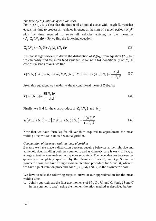
146

The time ZL(NL) until the queue vanishes.For ( )L LZ N , it is clear that the time until an initial queue with length NL vanishes

equals the time to process all vehicles in queue at the start of a green period (LN δ )

plus the time required to serve all vehicles arriving in the meantime( [ ( )]L L LA Z N δ ). So we find the following equation:

( ) [ ( )]L L L L L LZ N N A Z Nδ δ= + (29)

It is not straightforward to derive the distribution of ZL(NL) from equation (29), butwe can easily find the mean (and variance, if we wish to), conditionally on NL. Incase of Poisson arrivals, we find

[ ( ) | ] [ ( ) | ] [ ( ) | ]1

LL L L L L L L L L

L

NE Z N N N E Z N N E Z N N

δδ δλλ δ

= + ⇒ =−

(30)

From this equation, we can derive the unconditional mean of ZL(NL) as

[ ][ ( )]

1L

L LL

E NE Z N

δλ δ

=−

(31)

Finally, we find for the cross-product of ( )L LZ N and LN :

[ ] [ ]2[ ]

( ) [ ( ) |1

LL L L L L L L

L

E NE N Z N E E N Z N N

δλ δ

= =−

(32)

Now that we have formulas for all variables required to approximate the meanwaiting time, we can summarize our algorithm.

Computation of the mean waiting time: algorithmBecause we have made a distinction between queuing behavior at the right side andat the left side, handling both the symmetric and asymmetric case is easy. In fact, toa large extent we can analyze both queues separately. The dependencies between thequeues are completely specified by the clearance times CL and CR. So in thesymmetric case, we have a single moment iteration procedure for C and M, whereaswe have a joint iteration procedure for ML, CL, MR and CR in the asymmetric case.

We have to take the following steps to arrive at our approximation for the meanwaiting time:1. Jointly approximate the first two moments of ML, CL, MR and CR (only M and C

in the symmetric case), using the moment-iteration method as described before.

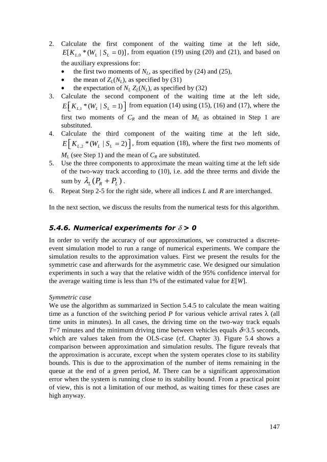
147

2. Calculate the first component of the waiting time at the left side,

,0[ * ( | 0)]L L LE K W S = , from equation (19) using (20) and (21), and based on

the auxiliary expressions for:• the first two moments of NL, as specified by (24) and (25),• the mean of ZL(NL), as specified by (31)• the expectation of NL ZL(NL), as specified by (32)

3. Calculate the second component of the waiting time at the left side,

,1 * ( | 1)L L LE K W S = from equation (14) using (15), (16) and (17), where the

first two moments of CR and the mean of ML as obtained in Step 1 aresubstituted.

4. Calculate the third component of the waiting time at the left side,

,2 * ( | 2)L L LE K W S = , from equation (18), where the first two moments of

ML (see Step 1) and the mean of CR are substituted.5. Use the three components to approximate the mean waiting time at the left side

of the two-way track according to (10), i.e. add the three terms and divide the

sum by ( )L R LP Pλ + .

6. Repeat Step 2-5 for the right side, where all indices L and R are interchanged.

In the next section, we discuss the results from the numerical tests for this algorithm.

5��-� �� /��δ�A�@

In order to verify the accuracy of our approximations, we constructed a discrete-event simulation model to run a range of numerical experiments. We compare thesimulation results to the approximation values. First we present the results for thesymmetric case and afterwards for the asymmetric case. We designed our simulationexperiments in such a way that the relative width of the 95% confidence interval forthe average waiting time is less than 1% of the estimated value for E[W].

Symmetric caseWe use the algorithm as summarized in Section 5.4.5 to calculate the mean waitingtime as a function of the switching period P for various vehicle arrival rates λ (alltime units in minutes). In all cases, the driving time on the two-way track equalsT=7 minutes and the minimum driving time between vehicles equals δ=3.5 seconds,which are values taken from the OLS-case (cf. Chapter 3). Figure 5.4 shows acomparison between approximation and simulation results. The figure reveals thatthe approximation is accurate, except when the system operates close to its stabilitybounds. This is due to the approximation of the number of items remaining in thequeue at the end of a green period, M. There can be a significant approximationerror when the system is running close to its stability bound. From a practical pointof view, this is not a limitation of our method, as waiting times for these cases arehigh anyway.

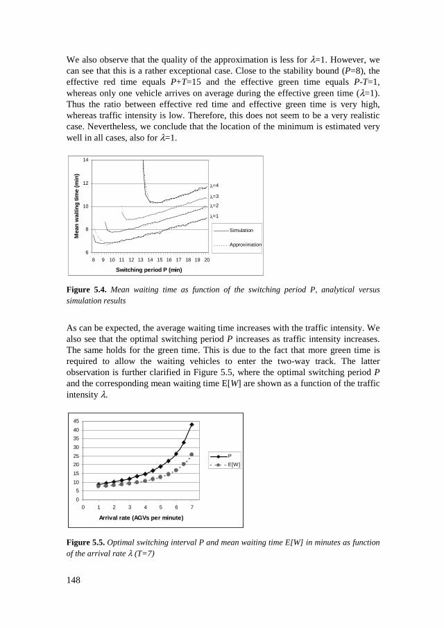
148

We also observe that the quality of the approximation is less for λ=1. However, wecan see that this is a rather exceptional case. Close to the stability bound (P=8), theeffective red time equals P+T=15 and the effective green time equals P-T=1,whereas only one vehicle arrives on average during the effective green time (λ=1).Thus the ratio between effective red time and effective green time is very high,whereas traffic intensity is low. Therefore, this does not seem to be a very realisticcase. Nevertheless, we conclude that the location of the minimum is estimated verywell in all cases, also for λ=1.

6

8

10

12

14

8 9 10 11 12 13 14 15 16 17 18 19 20

Switching period P (min)

Mea

n w

aitin

g tim

e (m

in)

Simulation

Approximation

λ=1

λ=2

λ=3

λ=4

Figure 5.4. Mean waiting time as function of the switching period P, analytical versussimulation results

As can be expected, the average waiting time increases with the traffic intensity. Wealso see that the optimal switching period P increases as traffic intensity increases.The same holds for the green time. This is due to the fact that more green time isrequired to allow the waiting vehicles to enter the two-way track. The latterobservation is further clarified in Figure 5.5, where the optimal switching period Pand the corresponding mean waiting time E[W] are shown as a function of the trafficintensity λ.

0

5

10

15

20

25

30

35

40

45

0 1 2 3 4 5 6 7

Arrival rate (AGVs per minute)

P

E[W]

Figure 5.5. Optimal switching interval P and mean waiting time E[W] in minutes as functionof the arrival rate λ (T=7)

149

Another interesting issue is the capacity of the two-way track. From equation (1), weobtain an upper bound for λ given a fixed value of P:

1 /

2

T Pλδ

−< (33)

The capacity equals 1/(2 )λ δ= vehicles per time unit for each side, but

unfortunately this level is reached if P→∞; in that case E[W] →∞. Therefore, amore realistic figure is the capacity of the two-way track given an upper bound onthe mean waiting time. Using the algorithm from Section 5.4.5, we conduct anumerical grid search over P and λ to find the maximum value of λ satisfying themean waiting time requirement. The results are shown in Figure 5.6, where thecapacity of the two-way track is expressed in λ, the number of vehicles to beprocessed per time unit at each side of the two-way track. We see that the capacityof the two-way track, given a maximum mean waiting time, seriously decreases withincreasing length, especially if only limited waiting time is accepted.

0

1

2

3

45

6

7

8

9

0 1 2 3 4 5 6 7 8 9 10

Driving time through tube T (min)

Max

. arr

ival

rat

e (A

GV

s/m

in.)

E[W]=5

E[W]=10

E[W]=15

E[W]=20

Figure 5.6. Two-way track capacity (number of vehicles per time limit per side of the two-way track), given a maximum mean waiting time

Asymmetric caseWe can also use the algorithm from Section 5.4.5 to calculate the mean waiting timeat each side of the two-way track as a function of the two switching periods, PL andPR. As an example, in Figure 5.7 we show the weighted mean waiting time

[ ] ( [ ] [ ]) /( )R R L L R LE W E W E Wλ λ λ λ= + + , based on the input data: T=7 minutes,

δ=3.5 seconds, λR = 2 per minute and λL = 3 per minute. This figure is a contourplot; it shows areas with similar values of the mean waiting time as indicated by thelegend. It is clear that the weighted mean waiting time increases faster with PR thanwith PL, given the higher arrival rate at the left side of the two-way track. Theoptimum is found around (PL, PR) = (11.75, 10.0), where the weighted mean waitingtime equals E[W]≈8.2

150

To give an indication of the accuracy of our approximation, we make a comparisonwith simulation results. The relative deviation between simulated and approximatedvalues, as function of PL and PR, is shown in Figure 5.8. The relative error is lessthan 1% for most of the cases. The error is somewhat larger close to the stabilitybounds, but as indicated before, this region is less interesting from a practical pointof view. The location of the minimum is slightly different for the simulated values:(PL, PR) = (11.25, 10.0). In our opinion, taking into account statistical fluctuationsarising from the discrete event simulation, this deviation is within reasonable limits.

7 8 9 10 11 12 13 14 15 16 17 18 19 207

8

9

10

11

12

13

14

15

P(L)

P(R)

E[W]

8-8.25 8.25-8.5 8.5-8.75 8.75-9 9-9.25 9.25-9.5 9.5-9.75

Figure 5.7. Approximation for the mean waiting time (weighted average of right and left side)as function of the switching periods PR and PL.

7 8 9 10 11 12 13 14 15 16 17 18 19 207

8

9

10

11

12

13

14

15

P(L)

P(R)

Deviation approximation vs. simulation (%)

0%-1% 1%-2% 2%-3% 3%-4%

Figure 5.8. Relative deviation between approximation and simulation results

151

5��6� B�� = ��"��

The method can be generalized to compound Poisson arrivals. In fact, the arrivalprocess has an impact only on a few characteristics to be discussed in this section. Ifwe modify these characteristics to account for other arrival processes and plug theseformulae into the expressions at the appropriate places, the algorithm still applies.We show that this can easily be accomplished for compound Poisson arrivals. Thatis, batches of vehicles arrive at the left (right) side of the two-way track according toa Poisson process with rate µL (µR), where the batch size has some discreteprobability distribution function DL (DR) with known mean and variance. Then it isstraightforward to derive that

[ ( )] [ ]( )L L R L L L RE A P P E D P Pµ+ = + (34)

[ ( )] [ ]( [ ])L R R L L L RE A P C E D P E Cµ+ = + (35)2 2 2[ ( )] [ ]( [ ]) [ ] [ ]L R R L L L R L L RVar A P C E D P E C E D Var Cµ µ+ = + + (36)

2[ ( )] [ ]( [ ] [ ])R L R R L L L R RE C A P C E D P E C E Cµ+ = + (37)

Further, we find from equation (29) that

[ ][ ( )]

1 [ ]L

L LL L

E NE Z N

E D

δµ δ

=−

(38)

2[ ][ ( )]

1 [ ]L

L L LL L

E NE N Z N

E D

δµ δ

=−

(39)

When using equations (34)-(39), we can still use our algorithm. When consideringfurther generalizations, for example to compound renewal arrivals, the expressionsbecome more complicated, because the memory-less property of the exponentialinter-arrival distribution is lost. We believe that it is still possible to generateapproximations for the expressions as mentioned above, but the quality of theapproximation has to be tested. This is a subject for further research.

)�) �8�7 :;�� 9��

In this section, we discuss the adaptive control rules in more detail. Subsequently,we address adaptive local control, adaptive look-ahead control and dynamicprogramming. For these control rules we present the case with δ=0 and δ>0. First,we introduce some notation:t0 = decision momentH = information horizon, i.e. at a decision moment t0, AGV arrivals up to

t0+H are known

152

C(t0) = the clearance time of the two-way track at t0, i.e. the time needed forthe last AGV to leave the two-way track, assuming that no additionalAGVs enter the two-way track (note that this definition is differentfrom the one used in Section 5.4)

tir; ti

l = the i-th arrival at the right (left) side of the two-way track, where tir

(til) ��0 if an AGV has already arrived

qr(t); ql(t) = the number of AGVs in queue at the right (left) at time t

5�5�� 7� ��

In this local control rule we consider the situation in which only the queue size ateither side of the two-way track is known. Without loss of generality, we assumethat the current driving direction is from left to right. In accordance with Section 5.3,we distinguish between two decision options: either the queue at the left passes thetwo-way track first or the queue at the right passes the two-way track first.

The case δ = 0A direction change, meaning that the AGVs at the right side will pass the two-waytrack first, will induce waiting time for the AGVs in queue at the left. These AGVsare forced to wait for at least a period equal to the clearance time (C(t0)) plus thedriving time (T). The waiting time caused by a direction change is:

( )TtCtqW lchange += )()( 00 (40)

When the direction is not changed immediately, but after the AGVs from the lefthave entered the two-way track, all AGVs in queue at the right have to wait longer.The waiting time per AGV equals the difference between the clearance time beforemaking a decision (C(t0)) and the new clearance time caused by AGVs entering thetwo-way track from the left. The new clearance time is equal to the driving time (T).Therefore, the cumulative additional waiting time for all vehicles in the queue at theright (qr(t0)) is:

( ))()( 00 tCTtqW rnochange −= (41)

The direction is changed immediately when Wchange < Wnochange. Otherwise, in a staticsituation the direction change is planned after all AGVs in the queue at the leftentrance have entered the two-way track. In a dynamic situation, it will be natural tomake a new decision when the next AGV arrives. Note that the waiting times for theAGVs at the right side of the two-way track caused by the clearance time areregarded as sunk costs; the waiting time already incurred at the decision moment isnot relevant.

153

The case δ > 0If δ > 0, an additional term has to be added to equations (40) and (41) to account forthe time it takes a convoy of AGVs to enter the two-way track. The first AGV inqueue can enter the two-way track directly, while all other AGVs have to remain ata distance δ from their predecessor.

{ }( )0,1)(max)()( 000 −⋅++= tqTtCtqW rlchange δ (42)

{ }( )0,1)(max)()( 000 −⋅+−= tqtCTtqW lrnochange δ (43)

When the convoy of AGVs enters the two-way track, new AGVs might arrive. Wedo not take these additional terms into account. Note that these formulas reduce to(40) and (41) when δ=0.

5�5�� 7� ��41 ��

Adaptive look-ahead control can be considered as an extension of adaptive localcontrol, taking into account future arrivals within the information horizon H. Let usconsider the cost functions associated with the decision options: changing thedirection at the decision moment or after the i-th arrival from the left.

The case δ = 0The cost function for the case where the two-way track direction is changed directlycan easily be found by a straightforward extension of formula (40):

{ }∑++≤

+−++=)(

000

00

)(,)(mintCTtt

lkchange

lk

tCTttCTtW (44)

Note that this equation reduces to (40) when tkl= t0. The formula includes the

waiting time of arrivals (tkl) at the left entrance of the two-way track up to

t0+C(t0)+T unless, given the restrictions set on the information horizon H, thisinformation is not available. Note how (44) also covers those situations in whichdecision making does not coincide with the arrival of an AGV (tk

l< t0).

The alternative is to postpone the change in direction. The direction change can bescheduled after the i-th AGV entering the two-way track. At that time qr(ti

l+T)AGVs are queuing at the right entrance. For each option costs are computed as:

( ) { }( )∑∑+<+<<

+−++−+=Ttt

rk

li

Tttt

lk

liinochange

li

rk

li

lk

li

tCttTttTtW )(,max2 002

, (45)

The first term considers the waiting times of AGVs arriving at the left side of thetwo-way track within the interval (ti

l, til + 2T), i.e., after i AGVs have entered the

two-way track and before the scheduled AGVs from the right have passed the two-way track. The second term of (45) represents waiting times for AGVs in the queue

154

and arriving at the right side of the two-way track up to a time horizon til + T.

Again, only arrivals within the information horizon H are taken into account. Thechoice of the number of options to be considered can be independent of theinformation horizon.

A straightforward comparison between the options is not possible, because wecompute waiting times for different schedules, each of which has its own planninghorizon. The moment that the last scheduled AGV leaves the two-way track isdifferent for all decision options. Thus the computed waiting time for each optioncorresponds with a different planning horizon. To facilitate comparisons we weighthe waiting times with the planning period. Weighted costs associated with eachoption are formulated as:

−+=

+=

0

,

0

2min

)(

tTt

WWC

tCT

WWC

li

inochangeinochange

changechange

(46)

The direction is changed immediately when WCchange < WCnochange. Otherwise thedirection change is planned after the i-th arrival which causes the minimumWCnochange (static situation) or may be postponed (dynamic situation). Anotherpossibility is to weigh by using the number of vehicles affected by the decision, butthen the total waiting time should be considered instead of only the additionalwaiting time.

The case δ > 0If δ > 0 additional terms have to be added which take into account the additionalwaiting time caused by the required distance between AGVs.

( ) ( ){ }( )∑

−+⋅+++≤

−+⋅++−−+⋅+++=1))(()(

0000000

0000

1))(()(,1))(()(mintCtqtCTtt

rlk

rchange

rlk

tCtqtCTttCtqtCTtWδ

δδ (47)

( )( )( )

{ }( )∑

∑

+−⋅+<

−+−⋅+⋅++−⋅+<<

+−+−⋅++

−+−⋅+⋅+−+−⋅+

=

Tittt

rk

li

TittqTitttt

li

rlk

li

inochange

li

rk

li

rli

lk

li

tCttTitt

TittqtTitt

W

)}1(,max{000

1))}1(,(max{2)}1(,max{00

,

0

00

)(,max)}1(,max{

1))}1(,(max{2)}1(,max{

δ

δδδ

δ

δδδ (48)

We assume that the number in the queue is greater than zero. Otherwise we have totake the maximum of qr(⋅)-1 and 0, as is shown in (42) and (43). The number ofoptions may increase as a result of the entrance time. The weighted costs associatedwith each option are formulated as:

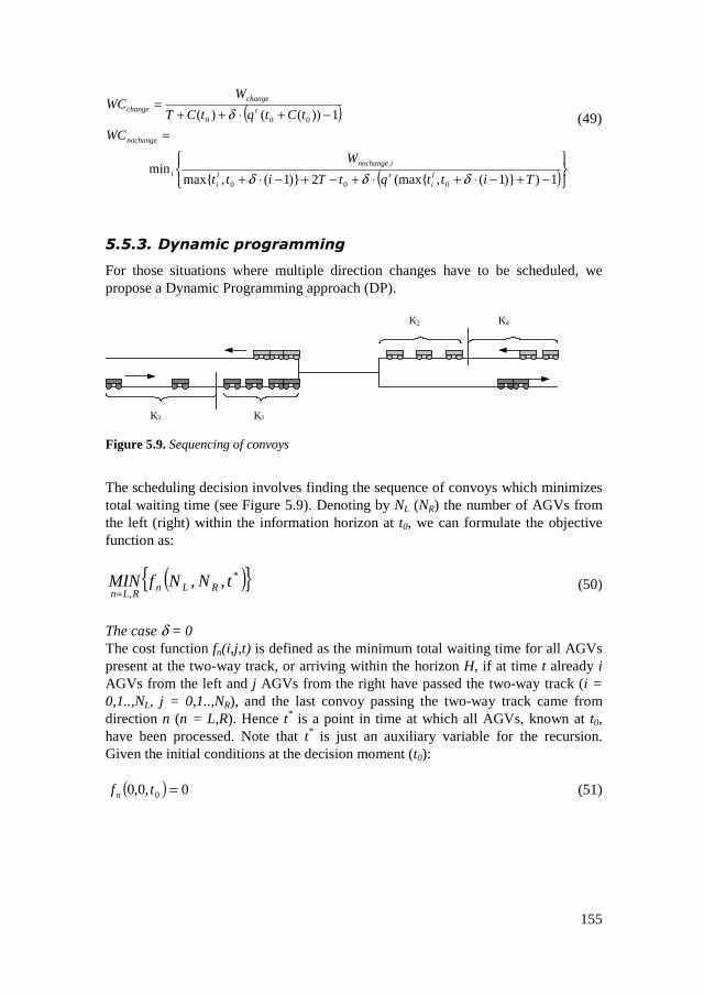
155

( )

( )

−+−⋅+⋅+−+−⋅+

=−+⋅++

=

1))}1(,(max{2)}1(,max{min

1))(()(

000

,

000

TittqtTitt

W

WC

tCtqtCT

WWC

li

rli

inochangei

nochange

r

changechange

δδδ

δ (49)

5�5�� #� ��

For those situations where multiple direction changes have to be scheduled, wepropose a Dynamic Programming approach (DP).

K1K3

K2 K4

Figure 5.9. Sequencing of convoys

The scheduling decision involves finding the sequence of convoys which minimizestotal waiting time (see Figure 5.9). Denoting by NL (NR) the number of AGVs fromthe left (right) within the information horizon at t0, we can formulate the objectivefunction as:

( ){ }*

,,, tNNfMIN RLn

RLn= (50)

The case δ = 0The cost function fn(i,j,t) is defined as the minimum total waiting time for all AGVspresent at the two-way track, or arriving within the horizon H, if at time t already iAGVs from the left and j AGVs from the right have passed the two-way track (i =0,1..,NL, j = 0,1..,NR), and the last convoy passing the two-way track came fromdirection n (n = L,R). Hence t* is a point in time at which all AGVs, known at t0,have been processed. Note that t* is just an auxiliary variable for the recursion.Given the initial conditions at the decision moment (t0):

( ) 0,0,0 0 =tf n (51)

156

The cost function fn(⋅) can be formulated, starting with the left side, as:

( ) ( ) ( )[ ] ( ){ }( ) ( ) ( )[ ] ( ){ }

( ) ( )[ ] { }

( ) ( )[ ] { }{ }{ }r

j

li

12

1221

22,..,1

21221,..,1

2

t,t’max’t’

tt,maxt’

0,’max’’,,,’,,

0,max’,,,,,

:

’,,’’,,,’,,min’’,,

,,’,,,,,min’,,

2

1

2

1

+=

+=

−=−

−=−−−

−+−=

−−+−−−=−

∑

∑=

+−=

=

+−=

=

=

T

T

tttjitkjic

tttkjitkjkic

with

tkjiftjitkjictjif

tkjkiftkjitkjkictkjif

jy

kjy

ry

iy

kiy

ly

Ljk

R

Rik

L

(52)

We assume that a convoy contains at least 1 AGV, without affecting optimality,because otherwise there is no reason to change the direction. The function c[(i-k1,j-k2,t),(i,j-k2,t’)] computes waiting times for a convoy of k1 AGVs that has entered thetwo-way track at time t and left it at time t’. This time is determined by the questionof whether the last AGV arrived during the red (ti

l≤t) or green period (til>t).

The computation times do not necessarily increase enormously with more arrivals,because not all discrete points in time have to be computed; the algorithm takes longtime steps of length T. AGVs that wait in queue when the traffic light becomesgreen will all enter the two-way track. It is not optimal to cut a queue into twoseparate convoys.

The case δ > 0In this case only the cost functions and the decision times change, the recursionremains unchanged.

( ) ( )[ ] { }

( ) ( )[ ] { }( ){ }( ){ }r

ir

li

l

122

11221

t,1)’(qt’max’t’

t,1)(qtmaxt’

0),2(’max’’,,,’,,

0),2(max’,,,,,

2

1

−⋅++=

−⋅++=

−+−⋅+−=−

−+−⋅+−=−−−

∑

∑=

+−=

=

+−=

tT

tT

kjytttjitkjic

kiytttkjitkjkic

jy

kjy

ry

iy

kiy

ly

δδ

δ

δ

(53)

Here we also neglect the fact that AGVs might arrive while the queue is entering thetwo-way track. Furthermore, we assume that arrivals at the two-way track satisfy thesame restrictions with respect to intermediate distances δ. In the implementation ofthe algorithm we assume that all AGVs that are waiting in the queue when the trafficlight switches to green enter the two-way track in one convoy. A queue is notseparated into two convoys, which might happen for a δ>0. This assumptionsignificantly reduces computation times.

157

)�0 ��:<�� 6��:=9� :�� 98?

To demonstrate the potential of the strategies for two-way track control, we set upan extensive simulation study. The design of the simulation study was based onfigures from the OLS-case (cf. Chapter 3). In this way, practical settings areguaranteed which may also serve as examples for future systems. In Table 5.3, theexperimental factors and their ranges are shown.

Table 5.3. Experimental factors

Factor Range1. Control rule PCR, ARloc, Arla, DP2. Average inter-arrival time (minutes) 0.5, 1, 1.5, 2, 43. Arrival distribution Poisson, Uniform4. Lot size 1, Uniform(3,9)5. Tube length (meters) 1000, 2000, 3000

For convenience, the control rules introduced in Sections 5.4 and 5.5 are abbreviatedas PCR (Periodic Control Rule), ARloc (Adaptive Rule with local control), ARla(Adaptive Rule with look-ahead), and DP (Dynamic Programming). Theexperimental factors concern the arrival patterns of AGVs (interval, distribution andlot size) and two-way track length. The driving speed of the AGVs is constant andequals 6 m/s. For each control rule average waiting time per AGV has beenmeasured for the default settings (marked boldly). Alternative system configurationswere chosen by changing the value of only one of the factors 2-5. For all controlrules we consider a dynamic setting where re-planning coincides with the momentone or multiple AGVs arrive at the two-way track and information changes or haschanged. The fixed time interval of the periodic control rule is determined by usingthe formulas derived in Section 5.4. We use the symmetric case (PL = PR) becausewe do not have information about arrival patterns at both ends. This results inchange-over times of 6.3, 6.8, 7.1, 7.3 and 8 minutes corresponding to average inter-arrival times of 0.5, 1, 1.5, 2 and 4 minutes.

For the adaptive look-ahead rule (ARLA), we chose to consider all options forchanging the driving direction within the interval [t0,t0+T]. Many choices arepossible here; our choice of the interval was motivated by two arguments. First,considering system characteristics, the driving time on the two-way track forms anatural horizon. Secondly, as a result of simulation experiments, we found that thechoice of the interval is an acceptable trade-off between the information requirementand the performance improvement. We assumed that the information on AGVarrivals would be available for a period equal to H = 3T, i.e., three times the drivingtime for the two-way track. This period logically follows from the above choice toconsider all possible moments for changing the two-way track direction up to oncethe driving time on the two-way track (T). Given a maximum clearance time of T,waiting times for AGVs may be influenced up to 3T. After a change of direction

158

they will not be able to enter the two-way track until the last AGV from the left andthe AGVs queuing at the right have passed the two-way track.

In addition to the experiments mentioned in Table 5.3, we studied the practical useof a DP-approach in somewhat more detail by means of a sensitivity analysis.Computation times were recorded and the effects of the planning frequency onsystem performance were studied. To get an idea of the effect of the planningfrequency, we tested the DP-rule for a smaller planning frequency. Furthermore, weconsidered the effect of the minimum distance between AGVs on systemperformance (δ > 0).

In our experiments we adopted the batch means method (cf. Law and Kelton, 1991;Hoover and Perry, 1989). Each batch equals one day. The first batch is discarded toaccount for any start-up bias. We related the number of batches to the relative width(γ = 0.01) of the confidence interval for the average waiting time, where thesignificance level α is set to 0.05. Lack of correlation of the batches was tested byusing the runs test (cf. Hoover and Perry, 1989). Given a significance level α = 0.05,this showed no significant correlation.

)�2 ��?�:��:=9� :��9 �

In this section, we analyze the outcomes of the simulation study. First, we presentresults for the default settings (Section 5.7.1). Next, we discuss how the choice ofalternative system configurations in terms of arrival distributions and two-way tracklength may influence system performance (Section 5.7.2). Sections 5.7.3-5.7.5consider the results of the sensitivity analysis concerning the length of theinformation horizon, computation times and the intermediate distance required forAGVs (δ > 0).

5�6��

In this section, outcomes of the simulation study are presented for the defaultsettings: single AGVs arriving according to a Poisson process at a 2000 meter longtwo-way track. In order to facilitate the comparison of the results, the performancefor each setting is indicated in terms of normalized average delay, i.e., the averagewaiting time at the two-way track divided by the driving time on the two-way track(T).

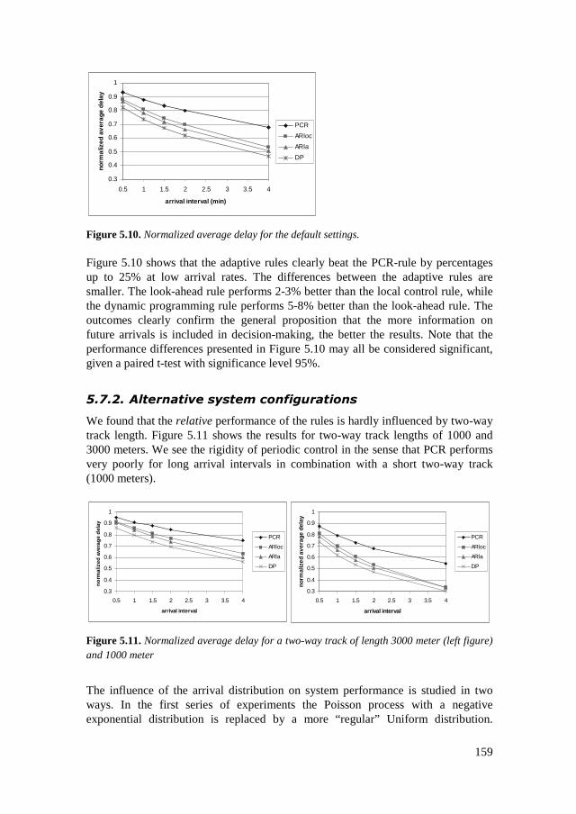
159

0.3

0.4

0.5

0.6

0.7

0.8

0.9

1

0.5 1 1.5 2 2.5 3 3.5 4

arrival interval (min)

norm

aliz

ed a

ver

age

del

ay

PCR

ARloc

ARla

DP

Figure 5.10. Normalized average delay for the default settings.

Figure 5.10 shows that the adaptive rules clearly beat the PCR-rule by percentagesup to 25% at low arrival rates. The differences between the adaptive rules aresmaller. The look-ahead rule performs 2-3% better than the local control rule, whilethe dynamic programming rule performs 5-8% better than the look-ahead rule. Theoutcomes clearly confirm the general proposition that the more information onfuture arrivals is included in decision-making, the better the results. Note that theperformance differences presented in Figure 5.10 may all be considered significant,given a paired t-test with significance level 95%.

5�6�� 7�� #��

We found that the relative performance of the rules is hardly influenced by two-waytrack length. Figure 5.11 shows the results for two-way track lengths of 1000 and3000 meters. We see the rigidity of periodic control in the sense that PCR performsvery poorly for long arrival intervals in combination with a short two-way track(1000 meters).

0.3

0.4

0.5

0.6

0.7

0.8

0.9

1

0.5 1 1.5 2 2.5 3 3.5 4

arrival interval

no

rmal

ized

ave

rag

e d

elay

PCR

ARloc

ARla

DP

0.3

0.4

0.5

0.6

0.7

0.8

0.9

1

0.5 1 1.5 2 2.5 3 3.5 4

arrival interval

norm

aliz

ed a

vera

ge d

elay

PCR

ARloc

ARla

DP

Figure 5.11. Normalized average delay for a two-way track of length 3000 meter (left figure)and 1000 meter

The influence of the arrival distribution on system performance is studied in twoways. In the first series of experiments the Poisson process with a negativeexponential distribution is replaced by a more “regular” Uniform distribution.

160

Although most results are comparable to those found for Poisson arrivals, relativeperformance differences between the control rules tend to be much smaller, usuallyless than 6% (see Figure 5.13). Secondly, we considered compound Poisson arrivals,where the lot-size of arriving AGVs is uniformly drawn from the interval [3,9]. Notethat we increased the average inter-arrival times (3, 6, 9 and 12 minutes)correspondingly. If results (Figure 5.12) are compared with those for the defaultsetting, two effects are apparent. First, a significant decrease in normalized averagedelay. Secondly, relative performance of PCR is worse. Both effects can beexplained by the fact that irregularity of arrivals is increased. In consequence of thelengthy arrival intervals on many occasions the two-way track will be idle.However, the irregularity makes on-line information more important; the two-waytrack direction should be changed when a convoy arrives. Clearly, a periodic controlrule will operate less efficiently under these circumstances.

00.10.20.30.40.50.60.70.80.9

1

3 6 9 12


no

rmal

ized

ave

rag

e d

elay

PCR

ARloc

ARla

DP

Figure 5.12. Normalized averaged delay for compound arrivals

Two conclusions can be drawn from this series of experiments:1. The greater the irregularity of the arrival pattern, the better the adaptive control

rules perform in comparison to the periodic control rule. This is due to theirresponsiveness to system state.

2. More irregular arrival patterns lead to lower normalized average delay. Morefrequently, large time gaps occur between AGVs, which are efficiently used bythe adaptive rules for changing the two-way track direction.

These conclusions are illustrated in Figure 5.13. The difference between theperformances of the periodic control rule and the dynamic programming rule ismuch smaller for Uniform arrivals, than it is for Poisson arrivals. We also see thatnormalized average delay is much smaller for Poisson arrivals, than it is for Uniformarrivals (cf. DP Poisson and DP Uniform). Similar conclusions were found byGlassey et al. (1991) in the context of dynamic machine scheduling.

161

0.4

0.5

0.6

0.7

0.8

0.9

1

0.5 1 1.5 2 2.5 3 3.5 4


no

rmal

ized

ave

rag

e d

elay

PCR Uniform

DP Uniform

PCR Poisson

DP Poisson

Figure 5.13. Periodic control and dynamic programming for Uniform and Poisson arrivals

In the previous experiments we considered the symmetrical case. However, if thearrival rates from the left and right side differ (asymmetric case), we expect that theperformance of the periodic control rule will be worse. This hypothesis wasconfirmed in an additional experiment. Given an average inter-arrival time of 0.5minutes from one side and 1 minute for the other side, the relative differencebetween the periodic control rule and the dynamic programming rule rises to 22%(compare Figure 5.10).

5�6�� ,��#�� =�� #

An interesting question from a practical perspective is how the performance of thenew control rules relates to the availability of information on future arrivals. Toanswer this question, we study the relationship between the length of theinformation horizon and system performance. In this section, we express theinformation horizon in meters rather than in time, because this naturally relates tofacilities for vehicle detection like sensors or inductive loops. The experimentincludes the DP-rule and the ARLA rule. As far as the DP rule is concerned, twoscheduling frequencies are considered: per arriving AGV (DP as considered inSection 5.7.1) and per convoy (DPconvoy). The scheduling frequency for theDPconvoy rule is related to a planned direction change, i.e. no new decision is madebefore the planned convoy has left the tube. The two-way track length is set to 2000meters, while AGVs arrive one by one according to a Poisson process with averagearrival intervals of 1 and 4 minutes. Figure 5.14 shows the numerical results, wherethe average inter-arrival time in minutes is given between parentheses. We see thatthe dynamic programming rule (DP) and the look-ahead rule (ARLA) are not verysensitive to the length of the information horizon. An information horizon of 3000meters already gives good results, while more distant information horizons do notlead to considerable improvement. The fact that performance is most influenced atlow arrival rates can easily be explained by the relative weight of information onarriving AGVs under these circumstances.

162

0.4

0.5

0.6

0.7

0.8

0.9

1

1000 2000 3000 4000 5000 6000 7000 8000

information horizon (meter)

no

rmal

ized

ave

rag

e d

elay

DPconvoy(4)

DP(4)

ARla(4)

0.4

0.5

0.6

0.7

0.8

0.9

1

1000 2000 3000 4000 5000 6000 7000 8000

information horizon (meter)

no

rmal

ized

ave

rag

e d

elay

DPconvoy(1)

DP(1)

ARla(1)

Figure 5.14. Sensitivity for the length of the information horizon and planning frequency forλ=1 (left figure) and λ=4 minutes respectively

Another effect, which is clearly shown by Figure 5.14, is the effect of the re-planning frequency in a dynamic context; compare the results for both DP rules.Clearly, a lower planning frequency can significantly reduce system performance.For longer information horizons, the effect is smaller.

5�6�� " �� "1 ��

The outcomes of the simulation study clearly point out dynamic programming as thebest performing heuristic for two-way track control. However, whether the dynamicprogramming approach is useful in practice also depends on the computationaleffort. A series of experiments indicated that even in the worst case evaluated in thesimulation study (see Section 5.6; average inter-arrival time of 0.5 minutes), thedynamic programming rule only requires a few seconds per changeover using aPentium III 500 MHz. Although computation times for the dynamic programmingrules tend to increase exponentially for higher arrival rates, this outcome still leavesa lot of room for practical application. This is especially true when one considers thefact that for high arrival rates the performance of the DP control rule is not verysensitive to the planning frequency (see Section 5.7.3).

5�6�5� 7B2�� #��

So far in the experiments we have assumed that the minimum distance between twosuccessive AGVs and the AGV length are negligible (δ=0). In this section we studythe effect of both factors on system performance. The parameter setting for theperiodic control rule is supported by the results from Section 5.4. This results inswitching periods of P = 8¼, 7½, 7, 6½, and 6¼ minutes corresponding to λ equal to0.5, 1, 1.5, 2 and 4 minutes. Figure 5.15 presents results for settings in which therequired distance between AGVs is set to 15 meters and the AGV length is 6 meters(δ = 3.5 seconds). The remaining settings correspond to the default settings. Theresults in Figure 5.15 are similar to those in Figure 5.10, although we clearly see theeffect of safety precautions in terms of longer waiting times in the case of hightraffic intensities.

163

0.4

0.5

0.6

0.7

0.8

0.9

1

1.1

1.2

0.5 1 1.5 2 2.5 3 3.5 4


no

rmal

ized

ave

rag

e d

elay

PCR

ARloc

ARla

DP

Figure 5.15. Intermediate distances and AGV length considered (δ =3.5 seconds)

)�, � A�/A�? ��E:��8�?� �=

5�C�� 3��#��#��

Until now we have studied the two-way track in isolation, as part of an open system.As a consequence, arrivals were considered independently of each other and aninfinite population was assumed. It is reasonable to assume an open system in thecase of a road network or a large transportation network. In these cases, the convoysthat are formed by the two-way track are dispersed to different destinations and thepopulation is also large compared to the traffic in the section under consideration. Ina closed system these assumptions can no longer be justified, making it necessary tostudy the effects of interaction with other elements in the network (compare theattention paid in the traffic literature to coordinating traffic signs, see e.g. Bell,1992). For example, let us consider the situation where the network at one side ofthe two-way track is a single terminal (see Figure 5.16). The convoys that leave thetwo-way track drive to the terminal, load/unload, and probably soon return to thesame two-way track. So the two-way track will face a batch arrival of AGVs, wherethe batch size is heavily influenced by a previous direction change. Decisions ontwo-way track control may therefore have serious impact on future decisions, aswell as having a significant impact on total system performance.

We consider a system in which there is a single terminal at one side of the two-waytrack (see Figure 5.16). The other side of the two-way track connects to a largetransportation network, such that arrivals at the left entrance are still independent.

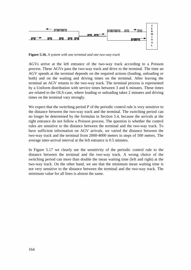
164

TERMINAL

Figure 5.16. A system with one terminal and one two-way track

AGVs arrive at the left entrance of the two-way track according to a Poissonprocess. These AGVs pass the two-way track and drive to the terminal. The time anAGV spends at the terminal depends on the required actions (loading, unloading orboth) and on the waiting and driving times on the terminal. After leaving theterminal an AGV returns to the two-way track. The terminal process is representedby a Uniform distribution with service times between 3 and 6 minutes. These timesare related to the OLS-case, where loading or unloading takes 2 minutes and drivingtimes on the terminal vary strongly.

We expect that the switching period P of the periodic control rule is very sensitive tothe distance between the two-way track and the terminal. The switching period canno longer be determined by the formulas in Section 5.4, because the arrivals at theright entrance do not follow a Poisson process. The question is whether the controlrules are sensitive to the distance between the terminal and the two-way track. Tohave sufficient information on AGV arrivals, we varied the distance between thetwo-way track and the terminal from 2000-4000 meters in steps of 500 meters. Theaverage inter-arrival interval at the left entrance is 0.5 minutes.

In Figure 5.17 we clearly see the sensitivity of the periodic control rule to thedistance between the terminal and the two-way track. A wrong choice of theswitching period can more than double the mean waiting time (left and right) at thetwo-way track. On the other hand, we see that the minimum mean waiting time isnot very sensitive to the distance between the terminal and the two-way track. Theminimum value for all lines is almost the same.

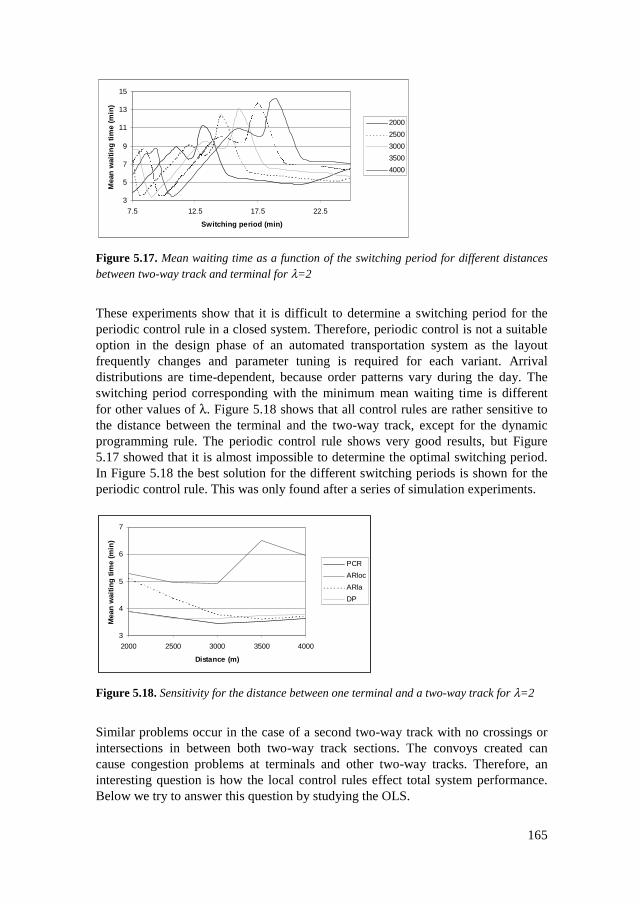
165

3

5

7

9

11

13

15

7.5 12.5 17.5 22.5

Switching period (min)

Mea

n w

aiti

ng

tim

e (m

in)

2000

2500

3000

3500

4000

Figure 5.17. Mean waiting time as a function of the switching period for different distancesbetween two-way track and terminal for λ=2

These experiments show that it is difficult to determine a switching period for theperiodic control rule in a closed system. Therefore, periodic control is not a suitableoption in the design phase of an automated transportation system as the layoutfrequently changes and parameter tuning is required for each variant. Arrivaldistributions are time-dependent, because order patterns vary during the day. Theswitching period corresponding with the minimum mean waiting time is differentfor other values of λ. Figure 5.18 shows that all control rules are rather sensitive tothe distance between the terminal and the two-way track, except for the dynamicprogramming rule. The periodic control rule shows very good results, but Figure5.17 showed that it is almost impossible to determine the optimal switching period.In Figure 5.18 the best solution for the different switching periods is shown for theperiodic control rule. This was only found after a series of simulation experiments.

3

4

5

6

7

2000 2500 3000 3500 4000

Distance (m)

Mea

n w

aiti

ng

tim

e (m

in)

PCR

ARloc

ARla

DP

Figure 5.18. Sensitivity for the distance between one terminal and a two-way track for λ=2

Similar problems occur in the case of a second two-way track with no crossings orintersections in between both two-way track sections. The convoys created cancause congestion problems at terminals and other two-way tracks. Therefore, aninteresting question is how the local control rules effect total system performance.Below we try to answer this question by studying the OLS.

166

5�C�� %!,1� ��

To check whether our conclusions for two-way track control in an open system areequally valid for a closed system, we embedded the rules in a simulation model forthe OLS (see Chapter 2). The layout that was studied contains one two-way track(cf. Figure 3.3). At one side of the two-way track there is only one terminal (VBA).At the other side the two-way track is connected to several terminals at AAS andRTZ. The two-way track has a length of 1500 meters and for both sides accurateinformation on arrivals is available by recording AGV movements 1500 metersbefore the entrance. Note that we shortened the two-way track to ensure thatsufficient arrival information is available. The required distance between two AGVsis 3.5 seconds. The control rules still aim to minimize the waiting time locally at thestart of the two-way track, but we measure the total system performance in terms ofthe service level, i.e. the percentage of transportation jobs that is handled before thedue time. Note that we take the same information horizon for both sides. This isalways possible if the minimum is taken from the information horizons. Usingdifferent horizons at each side is not a problem for PCR and ARLOC, but it mightinfluence the performance of the other two control rules. We did not investigate thiseffect.

The question is whether the local control rules that perform best in minimizing theaverage waiting time at an isolated two-way track also result in best systemperformance. For PCR after some initial experiments we chose a switching period of7 minutes. The simulation results confirm the ranking of the control rules withrespect to our performance measure, which can be seen in Table 5.4.

Table 5.4. Performance of the control rules in a closed system as in Figure 3.3

Control rule 180 AGVs 190 AGVsPCR (7 minutes) 90.2 99.7ARLOC 92.4 99.5ARLA 93.5 99.6DP 99.1 100

Note that for a closed system such as our application, we may adjust the control rule,e.g. by including information on the situation at the surrounding terminals and two-way tracks. The dock capacity of a terminal is known, together with the number ofjobs. A convoy that passes a two-way track and arrives at a terminal will incurwaiting time because of the restricted dock capacity. The length of the convoy isknown and also the number of unloading operations. With this information theexpected waiting time at the terminal can be estimated and these waiting times couldbe included in the control rules. We did not consider such a method because wefocus on local control. Furthermore, such an approach might be applicable in asituation with only one terminal at one side of the two-way track (see Figure 5.16)but is very difficult to generalize. The effects of a large convoy in a network with alot of terminals are difficult to estimate.

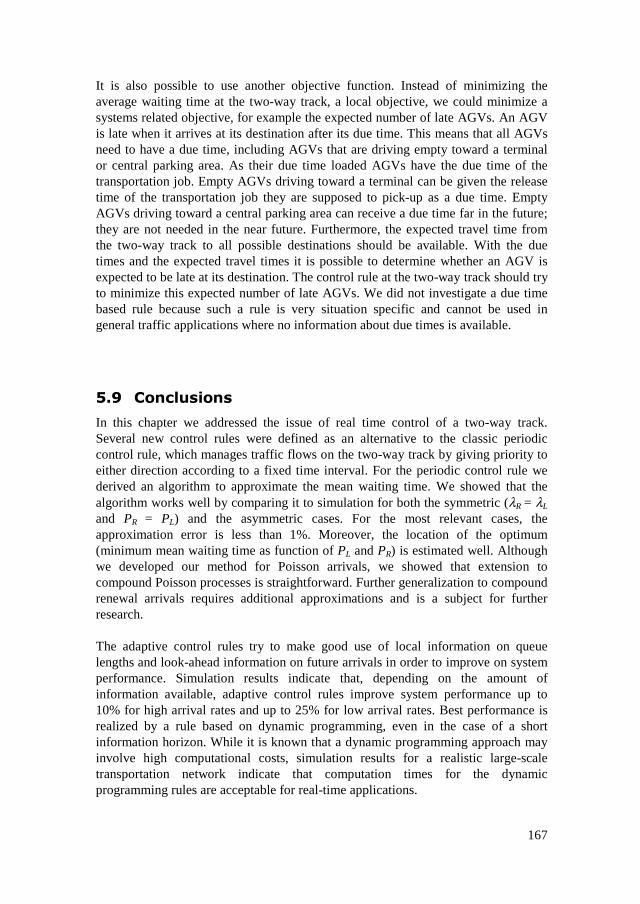
167

It is also possible to use another objective function. Instead of minimizing theaverage waiting time at the two-way track, a local objective, we could minimize asystems related objective, for example the expected number of late AGVs. An AGVis late when it arrives at its destination after its due time. This means that all AGVsneed to have a due time, including AGVs that are driving empty toward a terminalor central parking area. As their due time loaded AGVs have the due time of thetransportation job. Empty AGVs driving toward a terminal can be given the releasetime of the transportation job they are supposed to pick-up as a due time. EmptyAGVs driving toward a central parking area can receive a due time far in the future;they are not needed in the near future. Furthermore, the expected travel time fromthe two-way track to all possible destinations should be available. With the duetimes and the expected travel times it is possible to determine whether an AGV isexpected to be late at its destination. The control rule at the two-way track should tryto minimize this expected number of late AGVs. We did not investigate a due timebased rule because such a rule is very situation specific and cannot be used ingeneral traffic applications where no information about due times is available.

)�1 ��9�:��

In this chapter we addressed the issue of real time control of a two-way track.Several new control rules were defined as an alternative to the classic periodiccontrol rule, which manages traffic flows on the two-way track by giving priority toeither direction according to a fixed time interval. For the periodic control rule wederived an algorithm to approximate the mean waiting time. We showed that thealgorithm works well by comparing it to simulation for both the symmetric (λR = λL

and PR = PL) and the asymmetric cases. For the most relevant cases, theapproximation error is less than 1%. Moreover, the location of the optimum(minimum mean waiting time as function of PL and PR) is estimated well. Althoughwe developed our method for Poisson arrivals, we showed that extension tocompound Poisson processes is straightforward. Further generalization to compoundrenewal arrivals requires additional approximations and is a subject for furtherresearch.

The adaptive control rules try to make good use of local information on queuelengths and look-ahead information on future arrivals in order to improve on systemperformance. Simulation results indicate that, depending on the amount ofinformation available, adaptive control rules improve system performance up to10% for high arrival rates and up to 25% for low arrival rates. Best performance isrealized by a rule based on dynamic programming, even in the case of a shortinformation horizon. While it is known that a dynamic programming approach mayinvolve high computational costs, simulation results for a realistic large-scaletransportation network indicate that computation times for the dynamicprogramming rules are acceptable for real-time applications.

168

In general, the performance of the rules is not much influenced by the length of theinformation horizon. Only in the case of a low planning frequency (e.g. related tothe planned change-over times), is the dynamic programming rule sensitive to thelength of the information horizon. This effect is most noticeable at low trafficintensities. The introduction of safety precautions, such as the requirement that aminimum distance should be kept between AGVs to prevent collisions, does notsignificantly change the relative performance of the rules. Nevertheless, it doessignificantly change the optimum changeover time for the periodic control rule. Anexperiment that included the two-way track in a closed network, the OLS, showedthat our conclusions still hold for a closed system. We examine the robustness ofthese control rules to disturbances caused by equipment failures in Chapter 6(Section 6.3.5)

169

�6�7 ��

0

��8��?7�� ?��8��:9��=��<�=�� %��8 6�� :� �8� ��<�

��7��: :��

0�� 89� :��

In this chapter, we describe explorative research on some of the secondary processesin automated transportation networks that were introduced in Chapter 2 includingbattery management and failure management, and the management of the primaryprocess with restricted storage capacities. We describe only one possible way to takethese aspects into account in the control of the network and do not compare severalcontrol strategies. We want to show that the framework described in Chapter 2 isflexible enough to take these processes into account. Furthermore, we want toinvestigate the effects of constraints imposed by the secondary processes on thebehavior of the model, and the implications of these in the OLS-case. The inclusionof battery constraints is discussed in Section 6.2. We discuss how the results fromthis section can be used to choose a way of energy provisioning for the OLS-case. InSection 6.3, we describe the implications of failures of AGVs and docks. The effectsof restricted storage capacities, i.e. an additional bottleneck resource in the primaryprocess, are discussed in Section 6.4. Optimization of such control activities withinthe OLS-project strongly depends on technological choices still to be made.Therefore, the goal is to indicate the general effects and to highlight importantaspects that should be taken into account in answering some of the technological

170

questions. In this chapter we answer research questions 5 and 7 as stated in Chapter1 (Section 1.2.2). For all experiments in this chapter we use EVM3 (look-ahead rulewith hierarchical coordination, cf. Chapter 4, Section 4.4) for vehicle management.This control rule did not require adjustments when used in a system with two-waytubes. Two-way tubes themselves are controlled according to an adaptive rulewithout look-ahead, as discussed in Chapter 5, Section 5.4. This choice was madebecause the two-way tracks are close to the terminals; thus, there is little arrivalinformation available.

0�� ?=��<�=��

-�� .��

AGV battery replenishment or recharge is neglected in most studies on AGVsystems. Omitting battery constraints does not always have serious consequences(McHaney, 1995), particularly in internal AGV systems (production, warehousing)with short distances and with sufficient idle time to replenish or swap batteries.Nevertheless, in the case of high AGV utilization and long distances, these batteryconstraints cannot be neglected. McHaney (1995) also shows some examples inwhich the required number of AGVs significantly increased after the inclusion ofbattery constraints, and in some cases even doubled. In this section, we focus on theimplications of battery constraints for the logistic control. Furthermore, we presentseveral options for battery replenishment and show results for different strategiesand battery types.

We assume that the vehicles are driven by an electric motor (cf. Chapter 3). Adecision has to be made concerning the battery type: lead-acid or nickel-cadmium.Furthermore, there are several technical options with respect to batteryreplenishment:• a battery swap• recharging the battery inside the AGV• charge-rails

A battery swap strategy has limited influence on the operational time of the AGVs.The batteries are recharged outside the AGV. A disadvantage is the requirement ofspecial battery stations to execute the swap operation. Recharging the battery insidethe AGV means that an AGV is not available for several hours. In the OLS-case, therecharging time of a battery is longer than the possible driving time on a full battery,for a lead-acid battery recharging takes 8 hours, while the maximum driving time ona fully recharged battery is 6.4 hours (Van Harten et al., 1999). We do not considerthis option in this chapter, because it would more than double the required numberof AGVs. The same holds for recharging a nickel-cadmium battery inside the AGV.

171

The last option is charge-rails, where the AGVs are coupled to a charge-rail in partof the track network. The battery is recharged to such a level that the AGVs candrive freely in the other parts of the network (e.g. on the terminals). The option ofcharge-rails does not influence system performance because batteries arereplenished while AGVs are moving. An additional advantage of charge-rails,compared to swapping and recharging batteries, is that only as many batteries asAGVs are required, whereas additional batteries are required for the other twooptions. A drawback is the additional investment in charge-rails. In order to make aproper trade-off the results of our simulation studies can be coupled to a costanalysis. In Section 6.2.4, we give a hypothetical example of the way in which sucha trade-off can be made.

Logistic choices have to be made, depending on the chosen technical solution. Thequestions we want to answer with respect to battery management are:1. What are the implications of the technical solutions on the logistic control?2. What are the effects of the different technical solutions and battery types on the

logistic performance?3. Where should the battery stations be located?4. What are the required resources for the different options?5. What are rough indications for the costs of the different options?6. What is the most attractive solution with respect to costs and logistic

performance?These questions will be answered in the following sections.

-�� .�� #��

The introduction of battery constraints has implications for the logistic control. Wediscuss these implications for two options: a battery swap and charge-rails. Thebattery type and the option of charge-rails do not influence the logistic control. Inthe case of charge-rails, the only prerequisite is that the replenishment by charge-rails is sufficient to permit the AGV to drive freely in those parts of the networkwithout charge-rails. For the OLS-case, this condition is satisfied if charge-rails areconstructed in the tubes and AGVs only have to drive freely on the terminals. Nobattery stations are needed, but investments are required for the infrastructure on thetracks. In case of a battery swap, the AGV has to be sent to a battery station wherethe battery will be changed. Two questions have to be answered by the logisticcontrol. It is necessary to determine when and where the battery of an AGV shouldbe changed.

When?Three principles regarding the replacement of batteries can be considered. The firstoption is to replace a battery when its charge is not sufficient to perform the nextjob. An AGV receives a job from vehicle scheduling and checks whether its batterycharge is sufficient to complete the job. If the battery charge is not sufficient,

172

vehicle scheduling is notified. Vehicle scheduling has to determine whether anotherAGV should be used for the job, if not the selected AGV has to go to a batterystation while executing the job.

A second option is to change the batteries of all AGVs before a peak period. Such apreventive replacement of batteries is attractive from the point of availability when afully charged battery is sufficient for this peak. Unfortunately, this is not the case inthe OLS-system; batteries have to be changed at least once during the peak due tothe length of the peak period, therefore, we do not take this strategy into furtherconsideration.

Another option is to change the battery when an opportunity arises, i.e. a possibilityto change the battery when an AGV has to wait for some reason. Using suchopportunities could reduce the operational AGV time lost by battery changes but itdoes increase the number of battery swaps and so the battery swap stations shouldhave higher capacity. Opportunities arise when:• An empty AGV is temporarily parked at a terminal waiting for a new load job.

When an AGV is sent to a parking place, the battery manager is notified and,based on the charge information supplied by the AGV, can determine whether itis possible and useful, to change the battery of the AGV. It supposes that thereis a battery station at or near the terminal in question.

• An AGV has to wait at the entrance of a two-way track or terminal, due to thelimited capacity of such resources. When an AGV passes a sensor close to atwo-way track or terminal, it supplies information about its battery charge to thebattery manager. The battery manager can determine whether the battery can bechanged within the expected waiting time at the entrance of the terminal or two-way track, or by loosing only a fraction of the time normally required for abattery swap. This opportunity can only be used if there is a battery stationclose to the two-way track or terminal.

• An AGV that is on its way to or is at a central parking area. When an AGV issent to a parking area it is apparently not needed directly, so this is anopportunity to change the battery without seriously affecting the logisticperformance. In fact, this is a rather safe opportunity, as there are apparentlysufficient resources if an AGV is sent to a central parking area. However, theseopportunities do not occur during peak periods. Logically, a central parkingarea is an attractive location for a battery station.

• An AGV that is loading or unloading at a dock. If batteries can be replaced at adock while an AGV is being loaded or unloaded, the logistic performance is notinfluenced by this activity. Such a solution sounds attractive, but from atechnical point of view it is probably more difficult. Given the uncertainty aboutwhether it is technically possible, we do not consider this option in thisresearch.

173

Where?This decision covers the choice of locations for battery stations and, given that anAGV has to change its battery, the selection of one of the available battery stationsfor a battery change. In choosing locations for battery stations, the opportunitiesshould be taken into account (terminal, parking area, dock, and two-way track).Locations with high traffic intensity might be attractive as well. Besides logisticalreasons, costs and the available space are also important factors in determining thepossible locations for battery stations.

Given that an AGV has to change its battery, one of the battery stations has to beselected. Several heuristic rules are possible:• Nearest battery station• Farthest reachable battery station on the current route• First battery station encountered on the current route• Battery station that leads to minimum delay

The choice of where to change the battery depends on which battery stations canstill be reached. It must always be possible to reach the nearest battery station;otherwise, the battery should have been swapped during or before the previous job.In addition to the nearest battery station, other battery stations might also bereachable. One battery station should be selected from the set of reachable batterystations. It seems attractive to select a battery station on the route of the AGV. Whenthere are several battery stations on the current route one might want to minimizethe remaining charge of the batteries. In this case, battery management shouldchoose the farthest accessible battery station on the current route. When no batterystations are present on the current route, battery management can choose the batterystation that results in minimum delay for the job in question. Besides driving times,also the expected waiting time at a battery station could be taken into account.Somewhat different aspects play a role in case of an opportunity swap. In case of anopportunity at a terminal, where a battery has to be swapped within limited waitingtime, it is logical to use the nearest battery station to perform this battery swap. If anAGV is on its way to the central parking area, the choice of a battery station is lessimportant. However, when a battery station is located at the central parking area it islogical to use that one, if it can still be reached.

The OLS-caseFor the OLS-case, we first have to choose the locations of the battery stations. Thelayout with battery stations is shown in Figure 6.1, which was the preferred systemlayout at the time of research on battery constraints (Van Harten et al., 1999). Indetermining the possible locations of the battery stations, several criteria wereimportant. Based on opportunities, available space, traffic intensities, dispersionover the network and costs, three locations were selected. Because of the high trafficintensity between VBA and RTH and the location of these terminals at the networkboundaries, these locations seem logical. A central location near AAS seems a goodoption as well. As most waiting times (and hence opportunities) arise at the two-way

174

= battery station

= central parking

= terminal

tube, the location between the western terminal at AAS and the two-way tubebetween AAS and RTH seems preferable to a different location at Schiphol.Moreover, the central parking area is also planned at that same location. The threelocations indicated in Figure 6.1 might not be cost and space optimal for the batterystations, but no detailed information about costs and available space was available.The number of docks at a battery station is limited, but the recharging capacity, i.e.the capacity to recharge the batteries outside the AGVs, is unlimited.

Figure 6.1. Layout with two-way tracks and battery stations

The battery stations are located as follows: one battery station near the rail terminal,one battery station near the flower auction market, and one battery station close tothe central parking area at Schiphol Airport. With these locations, opportunities for abattery swap at the terminals RTH and VBA can be used, and the AGVs drivingtoward the parking area can also change their batteries. A terminal cannot handle anentire convoy (created by the two-way track) directly, and therefore waiting timesoccur at the entrances of the terminals. While waiting at the entrance, the batterycould be changed if a battery station was nearby. The effects of the number ofbattery stations are determined by a simulation study. We compare the case with 3battery stations with that where there is only 1 battery station at the central parkingarea.

Battery management is implemented as follows. When an AGV receives a new job,the AGV does not have to swap its battery if the remaining charge is sufficient todrive to its new destination and from this destination to the nearest battery station.When the remaining charge is not sufficient, the AGV is sent to the nearest batterystation to swap its battery. From this battery station, the AGV can carry on to itsdestination. We assume that both loaded and empty AGVs can swap the battery.Usually, the future destination of an AGV is not known. This means that an AGVthat is driving to a terminal will receive a new job (empty or loaded) at the terminal,

175

so whether the remaining battery charge is sufficient for this future job is also notknown. We choose to use a swap opportunity when the charge of a battery is notsufficient to drive from the current location to the farthest possible destination in thenetwork and from there to the nearest battery station, since this is rather robust interms of transport planning. AGVs will swap batteries more often than strictlynecessary, but the battery swaps can take place without real loss of time. An AGVthat drives to the central parking area changes its battery when the charge would notbe sufficient to drive from the parking area to the farthest possible destination andfrom there to the nearest battery station. The criterion of farthest possible destinationmight not always be appropriate. If one location is situated far from all otherterminals, this criterion might lead to unnecessary battery changes. A possiblesolution is to swap the battery if the charge is not sufficient for X% (e.g. 70%) of thejobs at that specific terminal.

Notice that these control rules for swapping batteries need estimates of the energyconsumption on all routes. These estimates have to be accurate, because an emptybattery, and as a result a stationary vehicle, has serious effects on the logisticperformance of the network in terms of throughput times and service levels (cf.Section 6.3 on failure management). The actual energy consumption on the routescan be recorded and average energy consumption is computed using an exponentialsmoothing technique (cf. Section 2.6). A safety factor is added to this average tominimize the chance that the AGV will fail to reach its destination. If in spite of thisthe AGV has to stop because of insufficient battery charge, it can be considered as afailed AGV, and therefore it has to be treated in the way as described in Section 6.3.

ExperimentsWith the simulation model, we investigated the effects of different options on thelogistic performance and resource requirements. We investigated different optionsfor battery replenishment, charge-rails or battery swap, and different variants withrespect to battery type (lead-acid, nickel-cadmium), number of battery stations andthe battery swap time (see Table 6.1).

Table 6.1. Experimental factors

Parameter OptionsBattery option Swap, charge-railsSwap time (min.) 1, 5Battery type Lead-acid, Nickel-cadmiumNumber of battery stations 1, 3

The swap time of 1 or 5 minutes was chosen after discussions with experts withinthe OLS-project in the field of automated docking and charging technology. If onlyone battery station is included, it is logical to choose the most central location: thebattery station near the parking area. Only one battery station reduces thepossibilities to use waiting times or AGV idle time for a battery swap. For theexperiments, we used the transportation flows from Table 3.2 in Chapter 3, together

176

with the general assumptions made in Chapter 3 with respect to speed, length of anAGV, etc.

Two options with respect to battery type were investigated, lead-acid batteries andnickel-cadmium batteries. For the nickel-cadmium battery we also consider a quick-charge option, which means that the battery is recharged up to 80% of its capacity,which can be done in 20% of the time for a complete recharge (see Table 6.2). Anadvantage of the nickel-cadmium quick-charge option is that fewer batteries areneeded in the system because of the short charge time. A big disadvantage is thatvehicles have to swap these batteries more often. In consequence, more batteryswapping capacity is required at the battery stations, order throughput times mayincrease and probably more vehicles are required to make up for this lost time. Thebattery charge capacity and required charging times of the battery types are shownin Table 6.2.

Table 6.2. Battery characteristics

Battery Capacity (kWh) Charge time (hour)Lead-acid 26.9 8Nickel-cadmium 17.9 5Nickel-cadmium quick-charge 13.1 1

We assumed that the recharging capacity of the battery charge stations, is not abottleneck, i.e. there are always fully charged batteries available when a vehiclewants to swap its battery. Nevertheless, the number of batteries recharging ismeasured in the simulation model to facilitate the cost computations. The rechargingtime of a single battery is proportional to the amount of charge that has to bereplenished.

The energy consumption of the batteries is not the same in all parts of the systemsince it depends on speed, status (loaded or empty), and also on possible slopes.Different figures are available for these cases, see Table 6.3 (Van der Heide, 1999).The energy consumption is independent of battery type, but driving in a two-waytube requires more energy than in a one-way tube, due to the convoys created in thetwo-way tube. Clearly driving up a slope requires a lot of energy.

177

Table 6.3. Battery consumption while driving

Status vehicle Consumption per hour (kWh)Empty in one-way tube (6m/s) 4.2Loaded in one-way tube (6m/s) 6.5Empty in two-way tube (6m/s) 6.8Loaded in two-way tube (6m/s) 9.0Empty on terminal (2m/s) 1.0Loaded on terminal (2m/s) 1.8Empty up-ramp (3m/s) 17.0Loaded up-ramp (3m/s) 31.0Empty down-ramp (6m/s) 0.9Loaded down-ramp (6m/s) 0.9

Moreover, we took the energy consumption for certain specific events into account.Acceleration requires additional energy, and at locations where AGVs alwaysaccelerate, for example at the exit of a terminal, or after a slope, this energyconsumption was taken into account (see Table 6.4). We did not take into accountthe energy used as a result of acceleration on a terminal.

Table 6.4. Energy consumption for acceleration

Event Consumption per event (kWh)empty accel. 2 -> 6 m/s 0.0177full accel. 2 -> 6 m/s 0.0322empty accel. 3 -> 6 m/s 0.0165full accel. 3 -> 6 m/s 0.0283empty accel. 0 -> 6 m/s 0.0194full accel. 0 -> 6 m/s 0.0356

-�� !�� #��

In this section, we show the results of the experiments defined in the previoussection. First, we determine the system dimensions with regard to the requirednumber of vehicles, number of battery stations and the number of docks in thesebattery stations. The results of this system without battery replenishment are equal tothe option of charge-rails. Using charge-rails means that batteries do not have to bechanged. The resource requirements are 8 docks at RTH and VBA, 2 docks perterminal at AAS and 360 AGVs (cf. Table 3.14); the loading and unloading time is 1minute. The number of docks in the terminals is kept constant because theintroduction of battery constraints has no real effect on these required capacities.Some preliminary experiments confirmed this statement. In Table 6.5, we show themost important results for the different options of battery replenishment. Thenumber of battery swaps influences the required docking capacity at the batterystations.

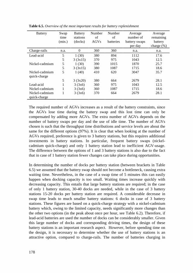
178

Table 6.5. Overview of the most important results for battery replenishment

Battery Swaptime

(min.)

Batterystations(docks)

Numberof

AGVs

Numberof

batteries

Averagenumber of

battery swapsper day

Averageremaining

batterycharge (%)

Charge-rails n.a. 0 360 360 n.a. n.a.Lead-acid 5 1 (30) 380 894 1112 17.6

5 3 (3x15) 370 975 1043 12.5Nickel-cadmium 5 1 (30) 390 1015 1870 25.7

5 3 (3x15) 380 1087 1715 18.6Nickel-cadmiumquick-charge

5 1 (40) 410 620 3047 35.7

5 3 (3x20) 380 664 2679 28.1Lead-acid 1 3 (3x6) 360 975 1043 12.5Nickel-cadmium 1 3 (3x6) 360 1087 1715 18.6Nickel-cadmiumquick-charge

1 3 (3x6) 370 664 2679 28.1

The required number of AGVs increases as a result of the battery constraints, sincethe AGVs lose time during the battery swap and this lost time can only becompensated by adding more AGVs. The extra number of AGVs depends on thenumber of battery swaps per day and the use of idle time. The number of AGVschosen is such that the throughput time distributions and service levels are about thesame for the different options (97%). It is clear that when looking at the number ofAGVs required, preference is given to 3 battery stations, but this requires additionalinvestments in battery stations. In particular, frequent battery swaps (nickel-cadmium quick-charge) and only 1 battery station lead to inefficient AGV-usage.The difference between the options of 1 and 3 battery stations is also due to the factthat in case of 1 battery station fewer changes can take place during opportunities.

In determining the number of docks per battery station (between brackets in Table6.5) we assumed that the battery swap should not become a bottleneck, causing extrawaiting time. Nevertheless, in the case of a swap time of 5 minutes this can easilyhappen when docking capacity is too small. Waiting times increase quickly withdecreasing capacity. This entails that large battery stations are required; in the caseof only 1 battery station, 30-40 docks are needed, while in the case of 3 batterystations 15-20 docks per battery station are required. A considerable decrease inswap time leads to much smaller battery stations: 6 docks in case of 3 batterystations. These figures are based on a quick-charge strategy with a nickel-cadmiumbattery which, owing to the limited capacity, needs significantly more changes thanthe other two options (in the peak about once per hour, see Table 6.2). Therefore, iflead-acid batteries are used the number of docks can be considerably smaller. Giventhis large number of docks and corresponding driving times, the design of thesebattery stations is an important research aspect. However, before spending time onthe design, it is necessary to determine whether the use of battery stations is anattractive option, compared to charge-rails. The number of batteries charging in

179

battery stations varies during the day, and is related to the transportation flows.From the number of batteries recharging at a battery station over 5 days, see Figure6.2, the necessary charging capacity of the battery stations can be computed. Thisgives an indication of the required number of locations at which batteries can berecharged outside the AGV. According to Figure 6.2, the required number of chargestations is about 500.

0

50

100

150

200

250300

350

400

450

500

550

600

1/0/00 12:00 AM 8/7/61 12:00 AMTime (5 subsequent days)

Nu

mb

er o

f b

atte

ries

Figure 6.2. Number of batteries recharging (lead-acid, 1 battery station)

The required number of batteries strongly depends on the chosen battery type. Quickcharging a nickel-cadmium battery can significantly reduce the required number ofbatteries (by 300-400). The effect of the number of battery stations on the requirednumber of batteries is a reduction of less than 10%. The positive effect of onebattery station is reduced by an increase in the required number of AGVs, alsobecause in this case less idle time can be used. The average remaining charge of abattery in absolute figures is not really different for the three battery types. This isnot the case when we look at percentages, because there is a big difference betweenthe capacities of the batteries. Part of the lost charge is caused by the chosen logisticcontrol rules. Battery changes are performed as much as possible in idle time, forexample when AGVs are waiting in front of a terminal. This leads to more frequentchanges, with on average more remaining charge, but less influence on systemperformance. A large part of the lost charge is caused by the long distances betweenthe terminals.

The number of battery changes largely depends on the net capacity of the batteryand less on the number of battery stations. If there are three battery stations,differences in the number of battery changes per station can be explained by theunbalanced transportation flows. Since most AGVs travel between RTH and VBA,many changes take place at these two locations. Most changing occurs at VBA, andthis can be explained by the fact that most AGVs travel loaded from VBA to RTH,and empty from RTH to VBA. Loaded trips require more battery charge, andtherefore more often a battery has to be changed before a loaded trip.

180

Decreasing the battery swap time has big positive effects. A battery swap time ofonly 1 minute diminishes the performance loss, but the battery swap still has seriousimpact on system performance. Shorter swap times make the option of quickcharging nickel-cadmium batteries competitive, because only a few extra AGVs arerequired to reach the demanded system performance. The result is that the requirednumber of batteries is substantially less than for the other options (see Table 6.5).Notice that with a swap time of 1 minute, combining the battery swap with theloading/unloading operations at a dock could be considered. This might betechnically complicated, but it would have positive effects on the logisticperformance. The performance is comparable with the option of charge-rails, and nobattery stations are required.

We conclude that all options have strengths and weaknesses from the logistic andfinancial points of view. In order to make a choice between the various options forenergy provisioning, in the next section we present an approach for the preparationof a cost analysis. Because of the lack of sufficiently accurate cost data, thecalculations are hypothetical.

-�� ,�� 1��

The choice of one of the technical options, (a battery swap or charge-rails), for oneof the battery types, lead-acid or nickel-cadmium, and the number of batterystations, cannot be based solely on logistical arguments. We present a way to assessthe costs of the different alternatives, based on artificial cost figures. More researchis required to estimate real costs, for example those of construction, vehicles andbatteries.

Table 6.6. Indicative costs for an automated transportation network

Costs (indicative) Description Unit Price/unit(x1000)

Battery Lead-acid piece 21.5

Nickel-cadmium piece 41.8AGV piece 150Terminal Loading/unloading dock piece 75Charging Charging location battery piece 12

Charge-rail in tube m 0.75

Battery station Battery station (space) m3 0.3Battery change dock piece 75

Maintenance Charge-rails, battery stations, charge locations, etc. P.M.

The costs of batteries, additional AGVs, battery stations, and charge-rails areincluded. The costs of battery stations include those of docks, space for storing andcharging batteries, and charge stations.

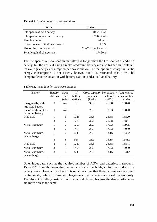
181

Table 6.7. Input data for cost computations

Data Value

Life span lead-acid battery 40320 kWh

Life span nickel-cadmium battery 57360 kWhPlanning period 20 yearInterest rate on initial investments 4.0 %Size of the battery stations 2 m3/charge location

Total length of charge-rails 17460 m

The life span of a nickel-cadmium battery is longer than the life span of a lead-acidbattery, but the costs of using a nickel-cadmium battery are also higher. In Table 6.8the average energy consumption per day is shown. For the option of charge-rails, theenergy consumption is not exactly known, but it is estimated that it will becomparable to the situation with battery stations and a lead-acid battery.

Table 6.8. Input data for costs computations

Battery Batterystations

Swaptime(min)

m3

batterystations

Gross capacitybatteries(kWh)

Net capacitybatteries(kWh)

Avg. energyconsumption

per dayCharge-rails, withlead-acid battery

0 n.a. 0 33.6 26.88 15820

Charge-rails, nickel-cadmium battery

0 n.a. 0 23.9 17.93 15820

Lead-acid 1 5 1028 33.6 26.88 158203 5 1210 33.6 26.88 15841

Nickel-cadmium 1 5 1250 23.9 17.93 159353 5 1414 23.9 17.93 16050

Nickel-cadmium,quick-charge

1 5 420 23.9 13.15 16452

3 5 568 23.9 13.15 16412Lead-acid 3 1 1230 33.6 26.88 15841Nickel-cadmium 3 1 1454 23.9 17.93 16050Nickel-cadmium,quick-charge

3 1 588 23.9 13.15 16412

Other input data, such as the required number of AGVs and batteries, is shown inTable 6.5. It might seem that battery costs are much higher for the option of abattery swap. However, we have to take into account that these batteries are not usedcontinuously, while in case of charge-rails the batteries are used continuously.Therefore, the battery costs will not be very different, because the driven kilometersare more or less the same.

182

0.00

1.00

2.00

3.00

4.00

5.00

6.00

7.00

8.00

9.00

10.00

11.00

Ch

arg

e ra

ils, l

ead

-ac

id b

atte

ry

Ch

arg

e ra

ils, n

icke

lca

dmiu

m b

atte

ry

Le

ad-a

cid

, 1 b

atte

ryst

atio

n, 5

m s

wap

tim

e

Lea

d-a

cid

, 3 b

atte

ryst

atio

ns,

5m

sw

aptim

e

Nic

kel c

ad

miu

m, 1

batte

ry s

tatio

n, 5

msw

ap ti

me

Nic

kel c

adm

ium

, 3ba

ttery

sta

tion

s, 5

msw

ap

time

Nic

kel c

adm

ium

qui

ck-c

ha

rge

, 1ba

ttery

sta

tion

, 5m

swap

tim

e

Nic

kel c

ad

miu

mq

uic

k-ch

arg

e, 3

batte

ry s

tatio

ns,

5m

swa

p tim

e

Lea

d-a

cid

, 3 b

atte

ryst

atio

ns,

1m

sw

aptim

e

Nic

kel c

adm

ium

, 3ba

ttery

sta

tion

s, 1

msw

ap

time

Nic

kel c

ad

miu

mq

uic

k-ch

arg

e, 3

batte

ry s

tatio

ns,

1m

swa

p tim

e

Co

sts

(mil

lion

gui

lder

s)

additional AGVs batteries battery stations charge rails

Figure 6.3. Cost comparison of the different alternatives

In Figure 6.3 we see the estimated costs for the different alternatives. The batteriesare responsible for the largest part of the costs, followed by charge-rails, batterystations and additional AGVs. The costs for the nickel-cadmium options are higherbecause this battery is assumed to be more expensive than a lead-acid battery. Thedifference in cost between charge-rails or a battery swap is not very great for thelead-acid battery. In this indicative example, the difference between 1 and 3 batterystations is small. The extra costs of 2 battery stations are comparable with the costsof additional AGVs in the case of only 1 battery station. From a cost point of view,quick-charging a nickel-cadmium battery seems to be more attractive than a normalcharging procedure. Overall, the charge-rails option is best, from both the logisticaland cost points of view, but a lead-acid battery swap follows closely.

-��5� +��

The main conclusions with respect to battery management are that:• Battery constraints in automated transportation networks should be considered,

because they can have a serious impact on the logistic performance and systemcosts, depending on the chosen option.

• The logistic control can be adapted to take battery constraints into account. Thelogistic control might be further optimized when some technical choices aremade.

• In the case of a battery swap strategy, these battery swaps should take place asmuch as possible during idle time or waiting time.

In making a choice between the replenishment options, the logistical implicationsshould be taken into account although of course, financial aspects should also beconsidered when choosing one of the replenishment options or battery types. Given

183

the results in the previous section and the fact that a lot of technical choices have yetto be made, in the rest of this chapter we assume that charge-rails are incorporated inthe system.

For the OLS-case, we conclude that:1. Given the relation between charging time and the driving time of a battery,

replenishing the batteries inside the AGV at battery stations is not a real option,.In the best case, the required number of AGVs increases with about 50%.

2. The best logistic performance can be obtained by using charge-rails, because noextra constraints are introduced.

3. With a battery swap time of 5 minutes, very large battery stations are requiredto reduce the effects on system performance. In this case the layout of thebattery stations becomes an important design question. Small battery stationslead to long waiting times and consequently to an increase in the requirednumber of AGVs or throughput times.

4. Decreasing the swap time to 1 minute leads to big improvements inperformance. Battery replenishment without serious performance loss is thenpossible.

5. In the case of a battery swap option a network with several battery stations is tobe preferred. Idle time can be exploited better and this leads to a smaller impacton the logistic performance. Because there are more battery stations feweradditional AGVs are required.

6. The additional number of batteries required for a battery swap strategy canincrease to twice the number of AGVs.

7. Based on the logistic performance, we would prefer a lead-acid battery. Thelarge capacity of this battery leads to less battery swaps. The use of a nickel-cadmium battery may be interesting when the battery swap time can besignificantly reduced.

0�' ��:9��=��<�=��

Failures can have serious consequences for the logistic performance of AGVsystems, but no literature was found on this topic. Besides speed, flexibility andenvironmental issues, the reliability of an automated transportation network is veryimportant. The resources most susceptible to failures are AGVs and docks. Suchfailures can have a serious effect on the logistic performance and therefore theycannot be neglected. A reason that we did not find something related in the literaturemight be the fact that in existing relatively small scale systems AGV failures can bequickly resolved. In an internal transportation system, a failed AGV can usually beremoved from the system in a few minutes, because it can be reached rather easily.Furthermore, if there are only a few AGVs and preventive maintenance is carriedout, AGV failures will be rare. In underground transportation systems, AGVs inunderground tubes are difficult to reach and it takes a considerable amount of time

184

to get them out of the tube; meanwhile the tube is blocked. Moreover, with a largenumber of AGVs, failures are no longer rare, but are an almost daily occurrence.

The objective of this section is to describe the design of control methods that canhandle the equipment failures of AGVs and docks. The model can be used todetermine acceptable failure rates, i.e. failure rates for docks and AGVs that onlyslightly influence the overall system performance, compared to the case withoutfailures. In the OLS-case, such acceptable failure rates derived from the simulationscan be used as targets in the design of AGVs and docks. Another option is todetermine the influence on system performance at a given failure rate. Electricityfailures, personnel failures and software failures are not taken into account; werestrict ourselves to AGV and dock failures. Questions we want to answer withrespect to failure management are:• What are the implications of failures for the logistic control?• What are the consequences for the logistic performance, depending on the

location of the failure and time of failure?• What are acceptable failure rates in the OLS-case?• Can additional AGVs compensate the effects of failures?

In Section 6.3.1, we describe the consequences of AGV and dock failures andpossible ways to handle these failures. In Section 6.3.2, we give the assumptionsmade in the OLS-case. To determine the effect of a specific failure, dock or AGV,given its failure location and the time of failure, we look at isolated disturbances inSection 6.3.3. Here the failure is dealt with as an isolated event and we determinethe system recovery time given a specific failure. A model with integrated failures isused in Section 6.3.4 to assess the logistic performance of the OLS system withfailures, and to determine acceptable failure rates. Furthermore, we investigate thedegree to which introducing a higher speed for a recovery vehicle or additionalAGVs can reduce the negative effects of failures. In Section 6.3.5 we investigate therobustness of two-way track control with respect to failures. In Section 6.3.6 wepresent the conclusions.

-�� :��

An AGV or dock failure influences the system for a certain amount of time. A faileddock cannot be used, which reduces dock capacity. A failed AGV possibly leads tolate delivery of the cargo on the AGV, but it also affects the operations in a part ofthe system. AGVs blocked behind a failed AGV have to wait until the failed AGV istowed or pushed away. Such a failed AGV can block a tube, a part of the terminal oreven an entire two-way track. Adequate and fast failure handling is thereforeimportant. In this section, we describe the modeling and control of AGV and dockfailures, starting with dock failures.

185

Dock failuresIn the case of a dock failure, the docking operation is stopped immediately. Thedock control object notices the dock failure and notifies the terminal manager. TheAGV that was involved in the dock operation is held up until the dock has beenrepaired. Other AGVs that are waiting at the dock might be able to drive around theAGV that is held up at the failed dock. The terminal manager has to take the dockfailure into account in local vehicle management, order release, and the taskallocation to docks. Local vehicle control takes action by no longer sending AGVsto that particular dock and rerouting AGVs already driving to the dock. Orderrelease cannot release new transportation jobs to this failed dock and task allocationto docks cannot assign a new functionality to the dock. Transportation jobs alreadyat the dock, or on their way to the failed dock, have to be recalled and sent toanother dock.

Repairing a dock takes a certain amount of time. After repair, the dock will restartthe loading/unloading operation it was working on at the time of failure. Thisoperation requires the normal loading or unloading time. When the dock isunblocked, the terminal manager is notified, and new jobs can be planned for therepaired dock.

AGV failuresHandling the AGV failures requires close attention. Failed AGVs should be repairedor taken out of the system as quickly as possible, because they block other traffic.Possibilities are to repair the AGV at the failure location or to bring the failed AGVto a repair station. Repairing an AGV in a tube is virtually impossible because thereis almost no space around the AGV. Moreover, the repair times will be veryunpredictable and other traffic is blocked for a long time. The other option is tobring the failed AGV to a repair station, towed by a recovery vehicle or pushed byother AGVs. In this case, choices have to be made with regard to the locations andnumber of repair stations. A terminal and a parking area are good locations for suchrepair stations.

Letting another AGV push a failed AGV might seem attractive, because the firstAGV that encounters the failed AGV can push the failed AGV to a repair station. Itseems that other traffic is not really influenced, but a failed AGV can still block atwo-way track for a long time, while waiting for another AGV to push it away.Furthermore, there should always be an AGV behind every other AGV; otherwise, itis possible that there will be no AGV to push the failed AGV. Other difficulties arisefrom a technical viewpoint. The AGVs have to be equipped with more powerfulengines to be able to push other AGVs, and it might not be possible to push a failedAGV at all, for example in case of a broken axle.

Recovery vehicles tow a failed AGV to a repair station. This means that specialvehicles are required and that these vehicles drive part of the route against the usualdriving direction to approach the failed AGV. Therefore, there should always be a

186

recovery vehicle in front of every AGV. In order to be able to reach the failed AGV,the tracks in front of the failed AGV should be freed of other traffic. All failedAGVs can be handled, because a failed AGV can also be lifted somewhat by arecovery vehicle, which might be necessary in case of a broken axle.

Both methods have their advantages and disadvantages, but the latter option ispreferred. It seems that this solution is most likely to be used within the OLSproject, because of the large number of AGVs in the network that have to beupgraded in case of the push approach. Therefore, we will investigate the effects offailures if a failed AGV is towed by a recovery vehicle. Once the failed AGV hasbeen taken out of the system, it can be repaired. In the remainder of this section, weuse the following general assumptions:• A failed AGV will be recovered by a recovery vehicle, which tows the failed

AGV to one of the repair stations.• Recovery vehicles do not fail.• There are sufficient recovery vehicles in the system, for example one at every

terminal.• A recovery vehicle can always reach a failed AGV, i.e. in case of two-way

tracks there should always be a recovery vehicle at both ends of the two-waytrack.

• We do not explicitly take the repair capacity into account; the repair process ismodeled by a repair throughput time that may consist of repair time and waitingtime.

In general, the recovery of a vehicle is modeled by using the following steps:1. Detecting an AGV failure2. Selecting the appropriate recovery vehicle and determining the route of this

recovery vehicle3. Preparing the recovery vehicle4. Clearing the route of the recovery vehicle5. Driving of the recovery vehicle to the failed AGV6. Towing the failed AGV to a repair station7. Handling the load when the failed AGV was loaded8. Repairing the failed AGV9. Returning the repaired AGV to the system

Figure 6.4 shows the communication between the objects involved, that results fromthe activities described above. Some of the activities give rise to a new controlobject; for example the selection of a recovery vehicle is done by failuremanagement.

187

Trafficcontrol

Recoveryvehicle

AGV

Failuremanagement

Vehiclemanagement

Terminalmanagement

1. AGV failed

1. AGV failure

1. AGV failure

4. Route clear 2. Clear route

5. Releaseroute

6. Make connection

7. Cargo needsfurther transport

5. Drive tofailed AGV

9. AGV repaired

6. Available fornext failure

2

3

Figure 6.4. Communication between the objects involved in failure handling

1. Detecting an AGV failureWhen an AGV breaks down, it can take some time before the failure is actuallydetected and the failure handling can start. The detection time depends on the failurelocation. If the AGV can still communicate, it notifies traffic control that it hasbroken down. Otherwise, traffic control should detect the failure based upon theexpected arrival time of AGVs at specific locations in the network. When an AGV islate at a specific point, it is necessary to check whether something has happened toit. In a terminal, a failure will probably be detected earlier than in a tube betweenterminals. Once traffic control knows about an AGV failure, failure management isinformed about the location and identity of the failed AGV, and it can start handlingthe failure. Failure management notifies vehicle management, because the failedAGV cannot be used for a long time.

2. Selecting a recovery vehicle and determining the routeWhen a failure is detected, failure management has to determine which recoveryvehicle will handle the failure. At the same time, the route of the recovery vehiclehas to be determined. The problem is that other AGVs may be driving in front ofand behind the failed AGV. We want to develop a strategy that can handle all AGVfailures at all locations in the network. It may be possible that the recovery can bespeeded up in very specific situations, for example when no AGVs are behind afailed AGV that is just outside a terminal. However, these situations will not occurfrequently during peak hours and they require very specific and exact informationabout the system state. Usually this information will not be available or will not beaccurate enough. In the chosen strategy, the failed AGV is always approached fromthe front. This means that a recovery vehicle drives part of the route against thenormal driving direction. In order not to disturb other traffic, an attempt is made totravel as far as possible in the normal driving direction. At the exit of a two-waytrack a recovery vehicle can change its driving direction once the route is cleared.

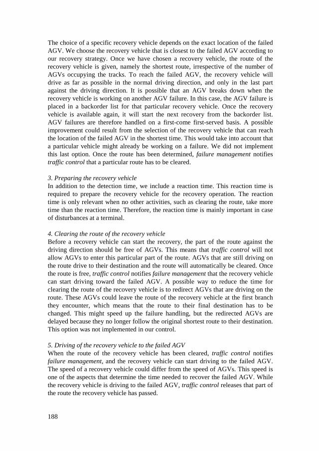
188

The choice of a specific recovery vehicle depends on the exact location of the failedAGV. We choose the recovery vehicle that is closest to the failed AGV according toour recovery strategy. Once we have chosen a recovery vehicle, the route of therecovery vehicle is given, namely the shortest route, irrespective of the number ofAGVs occupying the tracks. To reach the failed AGV, the recovery vehicle willdrive as far as possible in the normal driving direction, and only in the last partagainst the driving direction. It is possible that an AGV breaks down when therecovery vehicle is working on another AGV failure. In this case, the AGV failure isplaced in a backorder list for that particular recovery vehicle. Once the recoveryvehicle is available again, it will start the next recovery from the backorder list.AGV failures are therefore handled on a first-come first-served basis. A possibleimprovement could result from the selection of the recovery vehicle that can reachthe location of the failed AGV in the shortest time. This would take into account thata particular vehicle might already be working on a failure. We did not implementthis last option. Once the route has been determined, failure management notifiestraffic control that a particular route has to be cleared.

3. Preparing the recovery vehicleIn addition to the detection time, we include a reaction time. This reaction time isrequired to prepare the recovery vehicle for the recovery operation. The reactiontime is only relevant when no other activities, such as clearing the route, take moretime than the reaction time. Therefore, the reaction time is mainly important in caseof disturbances at a terminal.

4. Clearing the route of the recovery vehicleBefore a recovery vehicle can start the recovery, the part of the route against thedriving direction should be free of AGVs. This means that traffic control will notallow AGVs to enter this particular part of the route. AGVs that are still driving onthe route drive to their destination and the route will automatically be cleared. Oncethe route is free, traffic control notifies failure management that the recovery vehiclecan start driving toward the failed AGV. A possible way to reduce the time forclearing the route of the recovery vehicle is to redirect AGVs that are driving on theroute. These AGVs could leave the route of the recovery vehicle at the first branchthey encounter, which means that the route to their final destination has to bechanged. This might speed up the failure handling, but the redirected AGVs aredelayed because they no longer follow the original shortest route to their destination.This option was not implemented in our control.

5. Driving of the recovery vehicle to the failed AGVWhen the route of the recovery vehicle has been cleared, traffic control notifiesfailure management, and the recovery vehicle can start driving to the failed AGV.The speed of a recovery vehicle could differ from the speed of AGVs. This speed isone of the aspects that determine the time needed to recover the failed AGV. Whilethe recovery vehicle is driving to the failed AGV, traffic control releases that part ofthe route the recovery vehicle has passed.

189

6. Towing the failed AGV to a repair stationWhen the recovery vehicle reaches the failed AGV, they are coupled. The recoveryvehicle drives to the nearest repair station, leaves the failed AGV and receives a newdestination from failure management. Another option is to select a repair stationbased on how much effect the route to the repair station has on other traffic. If therecovery vehicle drives more slowly than the other AGVs when towing a failedAGV, the recovery vehicle should leave a busy route as quickly as possible in orderto minimize its effect on the other AGVs. We choose to send the recovery vehicle tothe nearest repair station and from there to its home base.

7. Handling the load when the failed AGV was loadedIt is possible that the failed AGV was loaded so the cargo should be delivered to itsfinal destination. We assume that it takes a specific time to unload the failed AGVand to prepare the cargo for further transport. It is possible that coincidentally thecargo is already at its destination. However, when the cargo is not at its destination,the cargo should be transported to the correct destination. Failure management willput this transportation job into the job list of the terminal. The transportation job willprobably receive high priority, because it was already being transported to itsdestination and time was lost because of the failure.

8. Repairing the failed AGVThe failed AGV is repaired in the repair station but it will not be available fortransport for several hours.

9. Returning the repaired AGV to the systemA repaired AGV should return smoothly into the system, i.e. the return of the AGVshould be announced to the information system so that it can again be used fortransportation jobs. The AGV returns in the system at the terminal at which it wasrepaired. The local empty vehicle manager is notified and can assign a new job tothis AGV. Because the repaired AGV is always empty, it can be used directly for anew transportation job, can be assigned to a parking place, or sent to anotherterminal or parking area.

Handling multiple AGV failuresThe recovery procedures described above work in the case of isolated disturbances,i.e. only one AGV breaks down, and in most cases of multiple disturbances.Nevertheless, there are situations that lead to a deadlock. It is possible that the routeof the recovery vehicle is blocked by another failed AGV, see Figure 6.5. Onerecovery vehicle wants to follow route 1 to recover failed AGV A at the right. Route1 is blocked by failed AGV B at the left side of the two-way track. This failed AGValso cannot be reached because failed AGV A blocks the route of the recoveryvehicle (route 2). We have a deadlock.

190

Route 1

Route 2

Failed

1

2

B A

Figure 6.5. Example of a deadlock situation in case of multiple failures

The two failures interfere with each other. Such situations can normally be solvedrather easily by human intervention. In the example above, a possible solution is thatrecovery vehicle 1 (at the left side) takes the other tube, that has to be cleared first.Then failed AGV A can be removed, and the problem is solved. However, not allpossible combinations of AGV failures can be easily generalized to one method forrecovery. Theoretically, the possibility of 3 or more simultaneous AGV failures inthe same part of the network cannot be excluded. With another recovery strategy,the deadlock depicted in Figure 6.5 might not have occurred, but in that case, alarger part of the system would have to have been cleared of traffic. In any case,these deadlock situations still have to be solved in our simulation model. Therefore,we introduce a special emergency method for these situations, which is put intoeffect when the failed AGV is not reached within a particular period of time. Weassume that within this particular time a solution has been found by humanintervention. After this maximum period, we assume that in one way or another, thefailed AGV has been reached and that it will move to the nearest repair station, at aspeed equal to that of the recovery vehicle. Notice that this emergency procedurewill not be called upon very often when the failure rate is low. Only in the case ofvery high hypothetical failure rates, would this emergency procedure be frequentlycalled upon. After an emergency has been handled, the recovery vehicle involvedcan start to cope with another failure.

-�� " ��%!,1� ��

To assess the implications of AGV and dock failures, we used the layout with two-way tracks (Figure 6.1), with the general input data with respect to transportationflows (Table 3.2), AGV speeds, terminals and throughput time requirements,described in Chapter 3. We made the following assumptions for our simulationstudy:• Failures are proportional with the operational time of AGVs and docks, i.e.

AGVs and docks only fail when they are active.• The time between two failures of the same object is exponentially distributed,

where the mean value is varied in our experiments.• There is a recovery vehicle on each terminal, combined with a repair station.• The repair time of a dock is exponentially distributed with an average of 1 hour.• The repair of an AGV takes 12 hours (deterministic).• The reaction time is 1 minute, recovery vehicles are always ready to handle a

failure.

191

• The emergency time, the maximum time until a failed AGV is reached by therecovery vehicle, is 7 minutes on a terminal, 20 minutes for a failure on a two-way track and 25 minutes for a failure at other locations. These times are basedon a worst-case of the time it might take to free the route of the recovery vehicleplus the time for the recovery vehicle to drive toward the failed AGV.

• Suppose that a loaded, failed AGV is towed to a terminal that is not its originaldestination. The time required to unload the cargo and prepare it for furthertransport is 15 minutes, starting from the arrival of the failed AGV in the repairstation.

• Batteries are charged by charge-rails; the batteries do not have to be changedand there are no battery stations in the model.

An AGV failure on a terminal is detected almost instantaneously because on theterminal communication is possible and personnel is present. When communicationis also possible in the tubes, the failure can also be detected almost instantaneouslythere, but otherwise an AGV failure outside a terminal or parking area is notdetected directly. Because there was no clarity on this issue at the time of ourresearch, we chose to assume that there would be no communication inside thetubes. Traffic control knows the expected arrival time of the AGV at specificlocations in the system (terminal, two-way track, etc.) and this information can beused to detect an AGV failure. When an AGV does not arrive at the specified time,or somewhat later (a safety margin), probably something has happened to the AGVand failure handling should be started. We therefore assume that the detection timeis equal to the remaining driving time that is needed to cover a part of the tube(track). Several sensors could be located in the tubes to reduce these detection times.

-�� 8/��

To investigate the effect of a disturbance on system performance, we first analyzedthe effect of an isolated disturbance. In fact, we controlled the conditions underwhich an AGV or dock fails (timing, location in the network), and investigated theeffects of such a specific failure. The logistic performance was measured by usingthe following performance indicators:1. the loss in service level on the day of failure (percentage of late orders).2. the recovery time, i.e. the time the system needs to reach a state that is

comparable with the state of the system without failure.

For the analysis of isolated disturbances, we designed a series of experiments forone of the OLS-layouts (Figure 6.1). We took the following aspects into account:a) Traffic intensity

• Outside the peak (Tuesday morning between 9.30 and 10.00)• Start of the afternoon peak (Tuesday afternoon between 12.30 and 13.00)• In the middle of the evening peak (Tuesday evening 19.00 and 20.00)

b) Speed of the recovery vehicle: 3, 6 and 12 m/sc) Location of the dock:

192

• At a busy terminal (RTH)• At a quiet terminal (AAS2)

d) Location of the failed AGV in the transportation system:• On a terminal (RTH): blocking the entry and on the middle of the terminal• On a one-way track (OWT), on a central location and between AAS1 and

AAS3• On a busy two-way track (TWT), the one between VBA and AAS3• On a quiet two-way track, between AAS1/AAS3 and AAS2

e) Position of the failed AGV in the convoy, i.e. first, second or one of the last.

We looked at the first and second AGV of a convoy, because these situations can bevery different. When the first AGV breaks down, the recovery vehicle can startdriving immediately, because the track in front of the failed AGV is already empty.When the second AGV breaks down, the first AGV has to clear the route, and thiscan take a while. In the meantime, this failed AGV is blocking the rest of theconvoy, which might have serious consequences. For other AGVs in the convoy thissituation occurs in a similar way, therefore we restricted the analyses to the 2nd

AGV.

Table 6.9. Twelve failure situations

Case Description

0 Base case: no failure

1 Dock on RTH, failed during one hour2 Dock on AAS2, failed during one hour3 AGV blocking entrance RTH4 AGV in the middle of RTH5 AGV on OWT AAS3-AAS1, first one in convoy6 AGV on OWT AAS3-AAS1, second in convoy

7 AGV on OWT AAS3-AAS1, last in convoy8 AGV on TWT AAS1-AAS2, first in convoy9 AGV on TWT AAS1-AAS2, last in convoy10 AGV on TWT VBA-AAS3, first in convoy, directly after entering the tube11 AGV on TWT VBA-AAS3, second in convoy, directly after entering the tube12 AGV on TWT VBA-AAS3, one of the last in the convoy

Summarizing, we had twelve different failure locations for AGVs and docks (c, dand e), see Table 6.9. Every failure situation was combined with three differenttypes of traffic intensity (point a) and three different recovery speeds (point b).Therefore, we had 108 different controlled disturbances. Notice that the experimentswere performed for a peak day (Tuesday) in an average week, so that the worst casewas included.

193

Results of the controlled failuresIn most cases, the impact of a single failure on the overall system performance interms of service level was rather marginal. The decrease in service level is usuallyless than 1 percent. However, in some cases we saw a serious negative effect. Thisoccurred especially if an AGV failed on the two-way track between VBA and AAS(cases 10-12). When the traffic intensity is high and the recovery speed low the losscan increase to 10 percent for a single bad failure. There also seemed to be an effectcaused by the recovery speed, especially when the recovery vehicle moves slowly (3m/s) leading to much delay and a poor performance. The additional improvement inperformance brought about by the use of a recovery vehicle moving at a higherspeed (12 m/s instead of 6 m/s) seems to be small.

The question is how robust these results are; they only represent one disturbance ona given day with a given stochastic realization. To investigate the robustness, wesimulated similar disturbances 4 times. Thus, we obtained an indication of thereliability and reproducibility of the results.

Table 6.10. Variation in performance loss

Case Description (i) (ii) (iii) (iv)

10 AGV on TWT VBA-AAS3, 1st in convoy 1.7% 1.3% 0.6% 4.5%11 AGV on TWT VBA-AAS3, 2nd in convoy 10.1% 2.7% 2.0% 8.1%

Table 6.10 shows the variation in performance loss for the two most serious cases,case 10 and 11. The same failure was simulated with four different sets of seednumbers for the random generators (variants (i)-(iv)). We saw that the effect of asimilar disturbance could vary greatly, especially for case 11. Therefore, theseisolated disturbances only gave an indication of the possible performance loss inparticular situations.

Despite the stochasticity in the effects of a controlled disturbance, it is interesting tosee how long it takes until the transportation jobs are no longer delayed, comparedto a run without disturbance. We looked at the number of delayed orders some timeafter the disturbance. The number of delayed orders was derived from the results ofthe same day without a disturbance. Most cases only had a small effect on thenumber of delayed orders. The system did not really run behind schedule and thusthere was no real recovery time. With the disturbance, the total process developedsomewhat differently, but was not really worse. In the most serious case (case 11(i)),the number of delayed orders was really large. In the evening peak, there was almostno time to recover from the failure. Only after 4 hours, when it was quiet again, didthe system seem to have recovered (see Figure 6.6).

194

0

25

50

75

100

125

150

0:00 0:30 1:00 1:30 2:00 2:30 3:00 3:30 4:00

Time after failure

Nu

mb

er o

f jo

bs

del

ayed

Figure 6.6. Recovery time case 11, in the middle of the evening peak, recovery speed 6 m/s

We also looked at the distribution of the delays of all orders after the disturbance.About 20% of the orders were still on time, while 95% of the orders had a delay ofless than 30 minutes. There were also orders that were delayed by 50 minutes ormore. Again, we see that this particular failure (case 11) had serious consequenceson system performance. The question is how often these serious disturbances occurin an automated transportation network and to answer this question, an integralanalysis is needed.

Conclusions for controlled disturbancesExperiments with isolated disturbances showed that the effect of a particulardisturbance is unpredictable and depends on many factors. Nevertheless, we canalready give some preliminary conclusions with respect to failures in automatedtransportation networks:1. Most disturbances only have a marginal effect on system performance, but

serious performance loss can occur in the case of a failure in a busy period at abad location. The recovery time of the system can accumulate to several hours.

2. The disturbances on a terminal (AGVs and docks) usually have only a limitedeffect. A failed AGV on a terminal can be taken out of the system relativelyquickly (within several minutes).

-�� 8/��

For integrated failures, we investigated the following variants:• The Mean Time Between Failures (MTBF) of AGVs is varied between 100 and

1500 operational hours.• The Mean Time Between Failures of docks is 10, 25 or 100 operational hours.• The speed of the recovery vehicle is 3, 6 or 12 m/s.

Failure behavior of docks and AGVs was first investigated separately. Afterwards,AGV and dock failures were integrated, and interaction effects could be

195

investigated. The simulation ran for a peak day with a run-length of 31 days, and thefirst day was deleted from the results to account for start-up effects. Furthermore,experiments were performed for an average week (Saturday to Friday), to seewhether the main conclusions from a peak day in an average month still held. For anaverage week the run-length is 71 days, i.e. 10 weeks.

Analysis of dock failuresFrom the transportation flows, we can easily derive a relation between the averagenumber of failures and the failure rate of the docks, without simulation. A MTBF ofdocks of 25 hours is equal to, on average, 3.7 dock failures per day, of which 0.7 atAAS, 1.7 at RTH, and 1.3 at VBA. Dock failures have only a marginal influence onthe throughput times, even in case of frequent disturbances (MTBF=10, on average9.1 failures per day). Besides throughput times we also looked at the effect of failurebehavior on the service levels, i.e. the number of orders that is on time at itsdestination. From Table 6.11 it can be concluded that dock failures only havemarginal effects on system performance.

Table 6.11. Effect of dock failures on the service levels (peak day in average week)

MTBF TOTAL

-- 97.2100 hour 97.025 hour 97.010 hour 96.4

Analysis of AGV failuresFrom the simulation results, we can compute some statistics with respect to AGVfailures, such as the average number of AGV failures per day. With an MTBF of1000 hours, there are on average 1.7 AGV failures per day. On a peak day, thisnumber can be three times larger. Furthermore, we can make a distribution of thefailures over the different parts of the system, i.e. parking area, terminals, on a one-way track and on a two-way track. We can also register the average time required tosolve an AGV failure. Table 6.12 shows that more than 80% percent of the failuresoccur outside a terminal or parking area. These failures are precisely the situationsthat, on average, require a long recovery time.

Table 6.12. Indication of the handling time of AGV failures, dependent on location

Location % failures Average handling time (min.)

One-way track 44% 18Two-way track 38% 20Terminal 12% 3

Parking area 7% 7

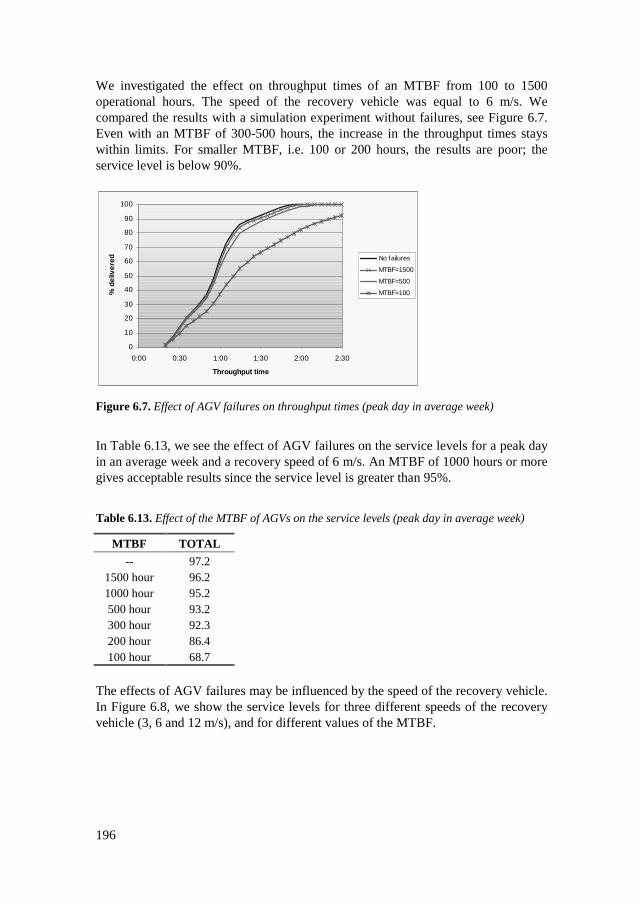
196

We investigated the effect on throughput times of an MTBF from 100 to 1500operational hours. The speed of the recovery vehicle was equal to 6 m/s. Wecompared the results with a simulation experiment without failures, see Figure 6.7.Even with an MTBF of 300-500 hours, the increase in the throughput times stayswithin limits. For smaller MTBF, i.e. 100 or 200 hours, the results are poor; theservice level is below 90%.

0

10

20

30

40

50

60

70

80

90

100

0:00 0:30 1:00 1:30 2:00 2:30

Throughput time

% d

eliv

ered No failures

MTBF=1500

MTBF=500

MTBF=100

Figure 6.7. Effect of AGV failures on throughput times (peak day in average week)

In Table 6.13, we see the effect of AGV failures on the service levels for a peak dayin an average week and a recovery speed of 6 m/s. An MTBF of 1000 hours or moregives acceptable results since the service level is greater than 95%.

Table 6.13. Effect of the MTBF of AGVs on the service levels (peak day in average week)

MTBF TOTAL

-- 97.21500 hour 96.21000 hour 95.2500 hour 93.2300 hour 92.3200 hour 86.4100 hour 68.7

The effects of AGV failures may be influenced by the speed of the recovery vehicle.In Figure 6.8, we show the service levels for three different speeds of the recoveryvehicle (3, 6 and 12 m/s), and for different values of the MTBF.

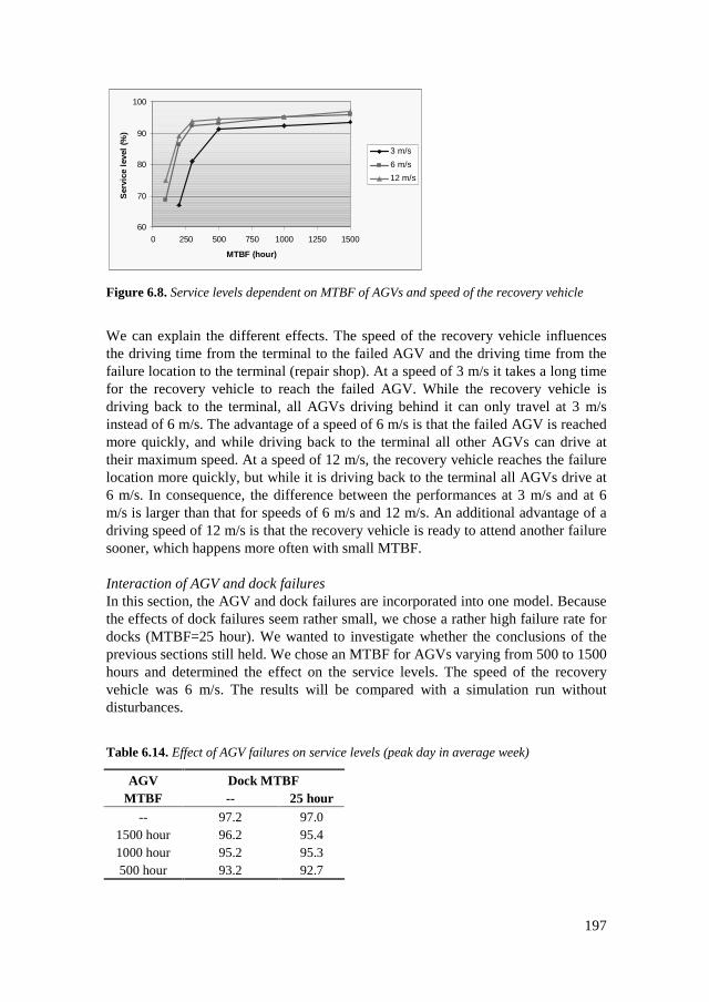
197

60

70

80

90

100

0 250 500 750 1000 1250 1500

MTBF (hour)

Ser

vice

lev

el (

%)

3 m/s

6 m/s

12 m/s

Figure 6.8. Service levels dependent on MTBF of AGVs and speed of the recovery vehicle

We can explain the different effects. The speed of the recovery vehicle influencesthe driving time from the terminal to the failed AGV and the driving time from thefailure location to the terminal (repair shop). At a speed of 3 m/s it takes a long timefor the recovery vehicle to reach the failed AGV. While the recovery vehicle isdriving back to the terminal, all AGVs driving behind it can only travel at 3 m/sinstead of 6 m/s. The advantage of a speed of 6 m/s is that the failed AGV is reachedmore quickly, and while driving back to the terminal all other AGVs can drive attheir maximum speed. At a speed of 12 m/s, the recovery vehicle reaches the failurelocation more quickly, but while it is driving back to the terminal all AGVs drive at6 m/s. In consequence, the difference between the performances at 3 m/s and at 6m/s is larger than that for speeds of 6 m/s and 12 m/s. An additional advantage of adriving speed of 12 m/s is that the recovery vehicle is ready to attend another failuresooner, which happens more often with small MTBF.

Interaction of AGV and dock failuresIn this section, the AGV and dock failures are incorporated into one model. Becausethe effects of dock failures seem rather small, we chose a rather high failure rate fordocks (MTBF=25 hour). We wanted to investigate whether the conclusions of theprevious sections still held. We chose an MTBF for AGVs varying from 500 to 1500hours and determined the effect on the service levels. The speed of the recoveryvehicle was 6 m/s. The results will be compared with a simulation run withoutdisturbances.

Table 6.14. Effect of AGV failures on service levels (peak day in average week)

AGV Dock MTBFMTBF -- 25 hour

-- 97.2 97.01500 hour 96.2 95.41000 hour 95.2 95.3500 hour 93.2 92.7

198

Table 6.14 suggests that there is a small interaction effect between AGV and dockfailures. The performance loss in the case of simultaneous failures is somewhatlarger than for both failures separately. It is also interesting to see how the servicelevels fluctuate from day to day, instead of only looking at an average number. Theresults are shown in Figure 6.9 and indicate the daily service levels for 30 peak daysin an average week, depending on the MTBF of AGVs (500 or 1500 hours) and anMTBF for docks of 25 hours.

80

82

84

86

88

90

92

94

96

98

100

0 5 10 15 20 25 30Day

Ser

vice

leve

l(%

)

No failures

MTBF=500

MTBF=1500

Figure 6.9. Fluctuations in service levels (peak days in average weeks)

In the case of low failure rates (large MTBF), the service levels are not only muchlarger, but also much more stable due to less failures. Nevertheless, also with a highMTBF bad days can happen. Even with an MTBF of 1500 hours, the service level isbelow 90% for one day. An AGV failure at a less accessible location and a busytime can lead to a performance decrease of 10% (see isolated failures). Such aserious disturbance can occur with all positive failure rates.

It may be possible that the negative effects of failures are partially or entirelycompensated by additional resources (AGVs or docks). Extra AGVs might lead to afaster recovery of the system. We looked at the effect of extra AGVs on the servicelevels. Because of the marginal effect of dock failures on system performance, wedid not look at the possibility of extra docks. Table 6.15 shows the results fordifferent numbers of AGVs.

199

Table 6.15. Service levels dependent on the number of extra AGVs

MTBF AGV 360 AGVs +10 AGVs +20 AGVs-- 97.2

1500 hour 95.4 96.0 95.81000 hour 95.3 95.6 94.6500 hour 92.7 94.4 94.8

The reduction in system performance resulting from failures can only becompensated slightly by extra AGVs. One reason is that more AGVs automaticallylead to more failures so in this case increasing the number of AGVs would not reallybe useful.

Effects for an average week (instead of a peak day in an average week)In this section we analyze the performance in an average week rather than just apeak day in such a week. We use an MTBF for docks of 25 hours and a speed of therecovery vehicle of 6 m/s in all cases. Table 6.16 shows the relation between theMTBF of AGVs and the service level in an average week. We see that the effects inan average week are much smaller. Even an MTBF of 500 hours leads to acceptableresults. The service levels fluctuate heavily between the different days (cf. Figure6.9). This is mainly due to the differences in transportation flows. Of course thebusiest days show the lowest performance.

Table 6.16. Effect of AGV failures on throughput times (all days in an average week)

AGV Service levelsMTBF AAS-

RTHAAS-VBA

RTH-AAS

RTH-VBA

VBA-AAS

VBA-RTH

TOTAL

-- 99.9 99.8 100.0 99.4 99.7 97.0 98.61500 hour 99.5 99.3 99.5 99.1 99.2 96.6 98.21000 hour 99.5 99.5 99.6 98.8 98.4 95.4 97.7500 hour 99.5 99.6 99.5 98.6 99.2 95.1 97.5

-��5� ��1� #�� 4��

In the previous sections we used the adaptive control rule without look-ahead fortwo-way track control (cf. Chapter 5). This rule only takes the information on queuelength into account, and is therefore probably less susceptible to failures. Failureslead to unreliable data on future arrivals, and given unreliable information, theadaptive control rule with look-ahead and the DP-rule might perform worse and takea bad decision for the actual situation. We investigated this effect in the system withone two-way track (cf. Chapter 3, Figure 3.3), with a length of 2800 meters. Theavailable information horizon was about 900 meters, equal to 2.5 minutes, given a

200

speed of 6 m/s. We used an MTBF of 500 hours for AGVs and an MTBF of 100hours for docks. For the periodic control rule we used a switchover time of 12minutes. In Table 6.17 we see the robustness of the two-way track control rules forthese failures.

Table 6.17. Robustness of the two-way track control rules, service level in case of failures

Control No failures Failures230 AGVs 250 AGVs 230 AGVs 250 AGVs

PCR 90.4 97.6 89.0 96.6ARLOC 95.8 98.0 94.3 97.9ARLA 94.3 97.8 79.8 91.2DP 97.2 98.4 94.4 97.9

The inclusion of failures has effects on the logistic performance, although theseeffects are smaller than in Section 6.3.4. This is due to a different system layout withonly one two-way track and a shorter length, which results in less AGVs. Theadaptive control rule with look-ahead is very sensitive to inaccurate information.When this rule is applied the performance of this rule drops seriously. The poorperformance is partly due to the short information horizon; this rule was designedfor a long information horizon. For the other control rules, PCR, ARLOC and DP, theperformance loss is limited to about 1%. The periodic control rule does not use anyinformation, and therefore is not influenced by inaccurate information; the loss ofperformance is entirely due to the failure process itself. More or less the same holdsfor the local adaptive control rule. For the case under consideration the informationabout queue lengths will be rather accurate, and therefore the periodic control rule isnot really influenced. The dynamic programming rule is less susceptible toinaccurate information than the look-ahead rule, but still we see a serious effect incase of 230 AGVs and failures. The performance of the DP-rule drops to the level ofthe local adaptive control rule. Therefore, the periodic control rule and the localadaptive control rule are robust with respect to AGV failures; these rules are notaffected by inaccurate arrival information. We can conclude that given itsrobustness, the simplicity and low computational costs a local adaptive control ruleseems well-suited for a system with failures.

It is important to mention that the performance of the information-intensive rulesmight be improved by notifying two-way track control about a failure, in which casetwo-way track control might switch to a local adaptive control rule. In such a case, itwould temporarily not use the probably inaccurate information.

We can also compare the results without failures with the results from Chapter 5.The ranking of the control rules is almost similar to the one found in Chapter 5. Theperiodic control rule performs worst, and the dynamic programming rule shows thebest results; significantly better than the rest. The adaptive control rule with look-ahead shows worse results than the local adaptive control rule, which can be a result

201

of the short information horizon. The dynamic programming rule appeared to be lesssensitive with respect to the information horizon (cf. Chapter 5).

-��-� +��

Here we highlight the most important conclusions from the previous sections:1. Failures cannot be neglected in modeling an automated transportation network;

in the OLS-case failure handling is a daily activity.2. Logistic control can be adapted to handle AGV and dock failures.3. In the OLS case, AGV failures have more impact than dock failures.4. Many disturbances have little effect on system performance, but one

unfortunate failure can result in a performance loss on one day of 10%.5. Failures on terminals have marginal effects on system performance because

they can be solved in little time.6. Additional AGVs can only slightly compensate for the loss in system

performance; the introduction of failures always leads to a lower logisticperformance.

7. The speed of the recovery vehicles should at least be equal to the speed of theAGVs. A lower speed is too slow and the effect of a higher speed seemslimited.

8. For the OLS case, the AGV failure rate should not exceed once per 500 activehours in order to preserve acceptable logistic performance.

9. A local adaptive control rule for two-way track control seems most robust withrespect to disturbances. The dynamic programming rule might still be the bestperforming rule after some slight modifications.

0�* �� :� �8� ��<��7��: :�� =:��

So far, we have neglected capacity restrictions on storage capacity at the terminals.Besides storage capacity restrictions, other capacity restrictions also exist (dockingand parking places). The latter two capacities are included in the simulation model,although the logistic control does not take these restrictions into account becausethey do not seem to cause an actual problem. AGVs can wait at the entrance of theRTZ and VBA terminal when there is no place inside. Only at the small Schipholterminals is there a lack of parking space. When this appears to be a bottleneck,these capacities should also be taken into account in the control. The consequence ofthe relocation of the rail terminal to Schiphol Airport (cf. Chapter 3, Figure 3.3) wasthat the storage space had to be limited because of very high costs and limited space.Therefore, these storage capacity restrictions should be taken into account. In thissection we want to investigate the effects of limited storage capacities and adapt thelogistic control to take these constraints into account. The OLS-layout with the railterminal near Schiphol is used in an example.

202

In the remainder of this section we use the following assumptions:• The terminals have separate in-buffers and out-buffers, each with their own

capacities.• Cargo remains in the out-buffer until the due time; at the due time the cargo

leaves the terminal by truck, train or plane. So space is occupied in the outbuffer from delivery at the destination terminal until the due time.

-�� 7��

Before going into more detail, we can state that the consequences of storagecapacity restrictions probably are:• More just-in-time control, which leads to less opportunities for peak shaving, so

probably more AGVs will be required.• More coordination between the terminals is required.• Cargo should be delivered in a specific order (order of departure from the

terminal of destination = departure of trains or planes).• Changes in order release: order release has to ask permission of the destination

terminal to release a specific transportation job.

A terminal with restricted storage capacity has to control the amount of cargo instorage. Cargo should arrive more or less in order of due time. A specifictransportation job with low priority (e.g. due time in 1.5 hours) should not occupythe storage space of a transportation job with high priority. In order to control thestorage on the terminal, the terminal manager needs to communicate with otherterminal managers. All terminal managers that want to start a transportation job,with another terminal as a destination, have to ask permission to start thetransportation job. If there is insufficient capacity, the destination terminal does notgive permission. When the destination terminal is able to receive new orders, itgives a signal to all terminals that new dispatch requests are allowed. To this end,each terminal manager maintains a storage occupation profile, describing theexpected storage utilization in the next period (say 1-2 hours) based on expectedload arrivals and departures.

The acceptance procedure by the destination terminal works as follows. Assume thatthe total storage capacity on terminal i is limited to C. The terminal manager canobtain information about all known transportation jobs that have terminal i as adestination, together with the due times of these jobs. For the first C transportationjobs on this list, sorted on due time, a place should be reserved in the cargo storage.When one of these C jobs leaves the storage (exits the system), another job can beunloaded. Therefore, when a request arrives from order release at terminal j to start atransportation job k with destination terminal i, the terminal manager has todetermine:• the number in storage (S);• the handling time for job k, τji

l, assumed to be deterministic;• the number of departures from storage before time t+τji

l: Nd(t+τjil);

203

• the number of transportation jobs that have higher priority than job k (higher onthe sorted list) and have not yet arrived: Na(k).

Transportation job k is allowed to start when: C – S + Nd(t+τjil) - Na(k) > 0.

The remaining capacity at time t plus the capacity that comes available before thearrival of job k, minus the capacity that has to be reserved for higher prioritytransportation jobs, should be larger than 0. Otherwise, all capacity is reserved fortransportation jobs with shorter due times. This means that orders do not have to bedelivered exactly in order of due time, as long as a place in storage is available forall (known) jobs with higher priority (shorter due time). It can still happen that atransportation job is delivered too early, because the travel times are not completelydeterministic. In that case, the AGV has to wait at a parking place or at a dock, untila storage location is available and it can be unloaded. A two-way track makes itdifficult to estimate the travel times. In this case, a safety margin should be includedto ensure that a transportation job is delivered at its destination before its due time.

The terminal manager of terminal i will notify the terminal manager of terminal jwhether transportation job k can be released. If the request is rejected, transportationjob k should be released at some other time in the future. The only times at whichthis is possible, is at moments when capacity comes available on terminal i.Therefore, when capacity becomes available on the terminal, terminal manager i willnotify all other terminal managers. At that moment these terminal managers canrequest permission to release transportation jobs for destination terminal i. Thecommunication can be reduced by informing only those terminal managers that areallowed to release transportation jobs. This will not affect the outcome of theplanning procedure.

The approach presented here works when only one terminal has a storage capacityrestriction. If several terminals have storage capacity restrictions, this method is nolonger guaranteed to work. It is possible that one terminal needs to send cargo toanother terminal, but that the receiving terminal has no cargo space available at thatmoment. Additional control rules are required to solve these conflicts. Possibly otherterminals with sufficient storage capacity could be used for temporary storage oreven a special storage facility could be introduced for this function.

-�� 3��%!,1� ��

The methods explained in the previous sections could be applied to all three systemdesigns. We chose the last system design, with internal transportation on SchipholAirport, but with the two-way track replaced by two one-way tracks, in order tohave (more or less) deterministic travel times. Failures are included in the model,with an MTBF of 500 hours for AGVs and 100 hours for docks, both exponentiallydistributed. The repair time for an AGV is 12 hours (deterministic), and the repairtime for a dock is exponentially distributed with an average of 1 hour. In allexperiments so far have we assumed that the storage space for cargo at the terminals

204

is unlimited. At Schiphol Airport the investment costs are very high and thereforethe terminals should be made as small as possible. To get an idea of the size of thestorage facilities on the terminals, we first measure the storage distribution perlocation, including the in-buffer and out-buffer, without taking into account finitestorage capacities.

Figure 6.10 shows the distribution of the storage capacity used on terminals RTZand VBA. We show the percentage of time that the storage capacity used is lowerthan or equal to the amount shown on the horizontal axis. It turns out that a storageutilization of more than 200 TU is rare at RTZ (about 10% of the time). At VBA for95% of the time there is less than 150 TU in the cargo storage. For most of the timethe storage capacity used at VBA is much lower than the storage utilization at RTZ.This is due to the logistic control, in which cargo is transported as quickly aspossible to handle most transportation jobs before the peak starts (peak shaving).Peak shaving reduces the required number of AGVs and it reduces the negativeeffects of two-way tracks. Now suppose that we restrict the storage capacity at RTZ.In consequence of such a storage capacity restriction at RTZ, the storage usage atVBA and AAS will rise. The total amount of cargo in the system remains the same,so it is just a matter of balancing loads over buffers.

.00%

10.00%

20.00%

30.00%

40.00%

50.00%

60.00%

70.00%

80.00%

90.00%

100.00%

10 30 50 70 90 110

130

150

170

190

210

230

250

Number in storage

% o

f ti

me

VBA

RTZ

Figure 6.10. Storage utilization, cumulative percentages in 2020, Tuesday with 250 AGVs

-�� 8�� %!,1� ��

We used the OLS-case to investigate the effects of limited storage capacities. Weassumed that the incoming and outgoing storage capacity at RTZ is equal to 80 TU,the choice of which was based on the number of docks in the terminal and theavailable space at each dock. The terminal at RTZ contains 16 docks, and at eachdock there is space for 5 outgoing TUs and 5 incoming TUs. For a technical solutionwith respect to docking technology, refer to Rijsenbrij et al. (2000). The otherterminals do not have storage capacity restrictions. We distinguished an incomingand an outgoing flow; the outgoing flow departs with the train and the incomingflow arrives with the train and is transported to other terminals in the OLS-system.

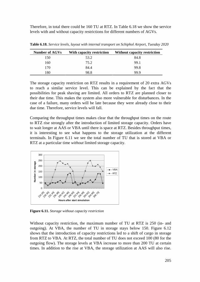
205

Therefore, in total there could be 160 TU at RTZ. In Table 6.18 we show the servicelevels with and without capacity restrictions for different numbers of AGVs.

Table 6.18. Service levels, layout with internal transport on Schiphol Airport, Tuesday 2020

Number of AGVs With capacity restriction Without capacity restriction150 53.2 84.8160 75.2 99.1170 84.4 99.8180 98.8 99.9

The storage capacity restriction on RTZ results in a requirement of 20 extra AGVsto reach a similar service level. This can be explained by the fact that thepossibilities for peak shaving are limited. All orders to RTZ are planned closer totheir due time. This makes the system also more vulnerable for disturbances. In thecase of a failure, many orders will be late because they were already close to theirdue time. Therefore, service levels will fall.

Comparing the throughput times makes clear that the throughput times on the routeto RTZ rise strongly after the introduction of limited storage capacity. Orders haveto wait longer at AAS or VBA until there is space at RTZ. Besides throughput times,it is interesting to see what happens to the storage utilization at the differentterminals. In Figure 6.11 we see the total number of TU that is stored at VBA orRTZ at a particular time without limited storage capacity.

0

50

100

150

200

250

300

[24,

26]

[28,

30]

[32,

34]

[36,

38]

[40,

42]

[44,

46]

[48,

50]

[52,

54]

[56,

58]

[60,

62]

[64,

66]

[68,

70]

Hours after start simulation

Nu

mb

er i

n s

tora

ge

VBA

RTZ

Figure 6.11. Storage without capacity restriction

Without capacity restriction, the maximum number of TU at RTZ is 250 (in- andoutgoing). At VBA, the number of TU in storage stays below 150. Figure 6.12shows that the introduction of capacity restrictions led to a shift of cargo in storagefrom RTZ to VBA. At RTZ, the total number of TU does not exceed 100 (80 for theoutgoing flow). The storage levels at VBA increase to more than 200 TU at certaintimes. In addition to the rise at VBA, the storage utilization at AAS will also rise.

206

The required storage capacity at some of the AAS terminals might double as a resultof the limited storage capacity at RTZ.

0

50

100

150

200

250

[24,

26]

[28,

30]

[32,

34]

[36,

38]

[40,

42]

[44,

46]

[48,

50]

[52,

54]

[56,

58]

[60,

62]

[64,

66]

[68,

70]

Hours after start simulation

Nu

mb

er i

n s

tora

ge

VBA

RTZ

RTZ-out

Figure 6.12. Storage with capacity restriction

-�� +��

In this section we showed a first approach to the incorporation of storage capacityrestrictions in the model. The logistic control was adapted to take these restrictionsinto account. These adaptations work in case of rather deterministic travel times,together with storage capacity restrictions at only one terminal. Nevertheless, theprinciples explained here can also be used with storage capacity restrictions atseveral terminals. Owing to capacity restrictions at several terminals, morecoordination is required between the terminals. If dock and parking capacities werealso incorporated in the logistic control, even more coordination would be required.In that case there would be so many restrictions that a scheduling approach wouldseem to be more appropriate. In Chapter 4 we showed a serial scheduling approachfor the vehicle management problem. It might be also possible to incorporate thesecapacity restrictions in such a method.

A disadvantage of the just-in-time principle is that the storage capacity utilization atthe other terminals increases. A possible solution is that the customers also delivertheir goods to the OLS just-in-time, and not 2 hours before train departure. Duringthese 2 hours, the cargo has to be stored somewhere in the OLS system. An option isto include a specific buffer facility in the network. Cargo could then be storedtemporarily at this facility when there was no space left at the terminals. Additionalactivities could take place at such a facility, such as the consolidation of cargoaccording to flight number or train compartment. A disadvantage of such a facility isthe additional number of transportation movements and the extra handling. Anotherdisadvantage of just-in-time control is that it becomes difficult when travel times arestochastic. Long two-way tracks cause great variations in travel times. The questionis whether these travel times can be predicted. Safety margins should probably be

207

incorporated to ensure that AGVs arrive at their destinations before the due time ofthe transportation jobs. The chance that an AGV arrives at its destination too earlywill also increase. More research is required to investigate whether two-way trackscan be incorporated in the previously described scheduling method. Ultimately, thiswould lead to a global optimization model in which we depart from the local controlconcept.

209

�6�7 ��

2

��9�:��8�9� 6��6

2�� 89� :��

Recent developments in the area of automated transportation networks provided themotivation for this research. In Chapter 1 we presented the research goal and theresearch questions to be answered in this thesis (Section 1.2.2). Let us now reflecton how the research questions have been answered. To start with we note that allmethods considered in this thesis conform to the real-time constraint stated in theresearch goal. Furthermore, we introduced several new elements in our research.Chapter 2 described the object model designed for automated transportationnetworks, based on a local control concept (cf. research question 3). This objectmodel was the basis for the development of an object-oriented simulation model ineM-Plant, which was used for experiments with control methods and system layouts,described in later chapters. The OLS-case, described in Chapter 3, is one that wasused to test the different control methods and options. In Chapters 4, 5, and 6, theresearch focused on the design and evaluation of control methods for severalimportant aspects of automated transportation networks. Vehicle management andtwo-way track control relate to the primary process, and for these primary objectswe developed several planning and control variants. We also developed controlobjects for the secondary processes, such as battery management and failuremanagement, in Chapter 6. In that chapter, we also examined the impact of storagecapacity restrictions on the system performance.

210

Summarizing, we developed a flexible logistic control structure that can be used forautomated transportation networks. Some of the developed control methods mayalso be useful in a broader context, such as fleet management problems (Chapter 4)and traffic applications (Chapter 5). A simulation library was designed to quicklyconstruct different system layouts and evaluate alternative control methods. Theseproducts proved very valuable in the OLS-case. We used the simulation library todetermine the logistical consequences of the ideas from several groups within theOLS project. For the OLS-case we showed that two-way tracks are feasible from alogistic point of view, resulting in significant savings, but with serious consequencesfor the logistic performance and resource requirements. Simulation results were alsoimportant input for the energy study and financial computations. The simulationlibrary is still used in the OLS project.

Turning to the new elements and answers to the research questions, in Section 7.2we discuss the conclusions relating to the topics discussed above. Topics for furtherresearch are discussed in Section 7.3.

2�� 9�:��

Object model and simulation model (research questions 1, 2, 4)In Chapter 2 we introduced an object model for automated transportation networks.In this object model, we made a clear distinction between physical, information andcontrol objects according to a logistic modeling framework. Furthermore, we made aclassification according to primary and secondary processes, transport and logisticactivities, and flow, handling and storage objects. By defining the control activitieswe answered research questions 1 and 4. We also described the performanceinformation that can be used to evaluate control methods. Performance measures toevaluate several methods for several control activities were further explored insubsequent chapters (cf. Chapters 4, 5, and 6).

The chosen approach proved useful, especially in evaluating methods for thedifferent planning activities, but also in the evaluation of system layouts. The resultis a simulation library in eM-Plant, which can be used to model automatedtransportation networks. New terminal designs, control methods (e.g. orderacceptance) and objects such as a load bearer, can be added to the library to increasethe options provided by the simulation library. The simulation library was used todetermine resource requirements for specific OLS system layouts, to determine theeffects of a two-way tube versus two one-way tubes, to evaluate a growth scenariofor the years 2005-2020, and to evaluate several methods for the control activities.

Though our object-oriented approach provides modular objects (building blocks),tuning of the control is always necessary. A specific combination of objects does notautomatically guarantee a good logistic performance. For example, a new vehicle

211

manager might require specific behavior from the terminal manager. Owing to thesedependencies, the construction of a model with good logistic performance is notalways straightforward. Performance is determined by the content and interaction ofobjects, not by an object-oriented structure.

Vehicle management (cf. research questions 4, 6, 8)For vehicle management, we designed several control rules, a First-Come First-Served heuristic, a rule with hierarchical coordination, a serial scheduling methodand an algorithm based on Powell and Carvalho’s logistic queuing networkapproach (see Table 4.1). These options were evaluated on customer service levels,resource requirements and empty travel distance. We can conclude that a simpleFCFS heuristic gives the worst results; all other rules yield significantly betterresults (see Table 4.5). In most cases, the local control rule with hierarchicalcoordination shows similar results compared to the rules with central coordination.Only in cases of demand that is quickly changing between routes and locations dothe rules with central coordination perform significantly better. The serialscheduling approach gave the best results, also with respect to empty travel distance,which means a reduction in energy consumption. The logistic queuing networkapproach shows slightly worse results than the rule with hierarchical coordinationand the serial scheduling approach. From these results, we can conclude that theperformance of a decentralized control rule is not necessarily worse than that of acentralized control rule. Only when the transportation flows are changing verydynamically, do the centralized control rules perform significantly better. Given thefact that we used a rather small network, it might be possible that in largertransportation networks the gap between centralized and decentralized controlincreases in favor of centralized control rules.

Pre-arrival information on transportation jobs improves the planning results, butinformation is only useful up to a certain time period (see Table 4.6). Given frequentre-planning, e.g. every 10 minutes, an information horizon equal to the maximumtravel time between two locations in the system (30 minutes in the OLS-case) seemssufficient. A longer information horizon only leads to marginal improvements(research question 6).

Two-way track control (research questions 4, 6, 8)A two-way track can considerably reduce infrastructure investment. Access controlrules were designed to manage vehicle flows, in such a way that collisions areavoided and waiting times are minimized. We developed both periodic control rulesand adaptive control rules that react to known and/or predicted vehicle arrivals (cf.research question 4). For the periodic control rule, theoretical approximations for themean waiting time as a function of the switching frequency were derived, for boththe symmetric and asymmetric cases (Section 5.4). Comparison with simulationresults indicated that the accuracy is usually in the range of 1-2% in the case ofPoisson arrivals. Based on these approximations, the optimum switching frequency

212

can be accurately approximated for a class of arrival processes (Poisson, compoundPoisson).

Intelligent adaptive rules vary from local adaptive control via look-ahead heuristicsto dynamic programming solutions. Numerical experiments showed that intelligentadaptive control rules reduce waiting times by 10-25% (see Figure 5.10), comparedto a straightforward periodic rule. In theory, the best adaptive control rule is adynamic programming rule, but this rule also requires the most intensive exchangeof information. It turned out that the dynamic programming method was not verysensitive to the information horizon, but in practice, it will probably be difficult togenerate the necessary information on future arrivals reliably. The less information-intensive, intelligent adaptive rules, even without look-ahead, can already realize thelarger part of the performance improvement (cf. research question 6).

Battery management (research questions 7, 8)From Chapter 6 (Section 6.2), we conclude that, unlike most internal transportationsystems, an automated transportation network cannot neglect battery constraints.Only when charge-rails are used, are the logistic effects of the use of batteriesnegligible, but this has the disadvantage that serious investment costs are required.The option of a ‘battery swap’ requires battery stations where batteries can beexchanged. Furthermore, the required number of AGVs slightly increases (up to10%) and the required number of batteries might even triple, depending on thebattery type and the possibility of using a quick-charge strategy. The logistic controlhad to be adapted to take battery constraints into account. AGVs have to be sent tobattery stations before the battery is empty, and whenever possible changing thebattery should take place during idle or waiting times. Additional AGVs cancompensate the negative effects of a battery swap strategy. The choice between oneof the alternatives, charge-rails or battery swap, and of a specific battery type (lead-acid or nickel-cadmium), cannot be based solely on logistic aspects. Detailed costcomputations are also required to support such a choice. We showed an approach toassessing the costs of the different alternatives (Section 6.2.4), which can be usedwhen detailed cost figures are available.

Failure management (research questions 5, 8)Handling AGV failures is a daily activity in a system such as the OLS, with seriousconsequences for the logistic performance, as shown in Section 6.3. We designedcontrol methods to handle AGV and dock failures, and to try to minimize thenegative effects of these failures. The model can be used to assess the effects ofgiven failure rates, or to determine acceptable failure rates, i.e. failure rates that donot really affect the logistic performance and could be used as a target in the designprocess. For the OLS case, we found that AGV failures affect the systemperformance much more than dock failures. When the AGV failure rate is smallerthan once per 500 operational hours, the decrease in system performance remainswithin reasonable limits. We only performed explorative research on failures. Fromexperiments with isolated controlled disturbances, we found that one AGV failure in

213

a two-way tube in a busy time period can reduce service levels for that particularday by 10%. Dock failures and AGV failures on terminals have only limited effectson system performance. In general, logistic performance decreases after theintroduction of failures. Additional AGVs can only slightly compensate thesenegative effects.

Storage capacity restrictions (research questions 4, 8)Several capacity restrictions can be present in automated transportation networks.The number of docks, parking places and storage locations is limited. Dock andparking capacities are included in the model, but not taken into account in thelogistic control. These capacity restrictions appeared to have limited impact onsystem performance, which can also be derived from the marginal effects of dockfailures. The storage capacity restriction was the most important capacity restrictionin the OLS-project at the time of the research. Owing to the very high investmentcosts at Schiphol Airport, storage space at the Zwanenburg rail terminal had to belimited. We extended the control methods to take this restriction into account,assuming that travel times vary only slightly (Section 6.4). The coordinationbetween the terminals has to increase when storage capacities are included. Giventhe fact that between arrival and departure cargo has to be stored somewhere in thesystem, a decrease in storage utilization at one terminal leads to an increase on otherterminals. Furthermore, a restriction on storage capacity reduces the possibilities forpeak shaving. As a consequence, the resource requirements increase. Furtherresearch has to be performed to investigate whether the same procedures can be usedwith stochastic travel times (see Section 7.3).

Impact of information (research question 6)The availability of information was an important aspect in this research. It turnedout that limited pre-arrival information, of about 15-30 minutes, improves thelogistic performance significantly (cf. Table 4.6). In controlling two-way tracks,information on future arrivals can also be used to reduce the waiting times at thesetwo-way tracks.

Another aspect is the accuracy of the information. The transportation flows used inthe OLS-case were estimated for the years 2005-2020. It is difficult to estimate thesetransportation flows, especially because there is not even a rail terminal at themoment and also, the throughput time requirements, which are still very unclear,were not known at the time of the research project. Therefore, the outcomes of thesimulation model with respect to the number of AGVs and docks are not exactanswers. Just as the inputs are estimates for 2020, the outcomes are alsoapproximations of the performance and resource requirements in the year 2020. Thestrong feature of the simulation model is that several scenarios or growth paths caneasily be computed. The model does not have to be changed; all methods work ifother transportation flows are introduced. Recall, for example, that the threedifferent system designs were substantially different, but that the methods developedwork for all these system designs.

214

2�' �9� 6��6

In Chapter 1, we made some assumptions and simplifications for the research in thisthesis. Several interesting topics for further research, partly based on the adaptationof these assumptions, are discussed in this section.

Capacity restrictionsA topic already mentioned in the previous section is the problem of capacityrestrictions. A method to incorporate storage capacity restrictions was discussed inChapter 6, but dock and parking capacities are not integrated in the logisticplanning. The small Schiphol terminals, without parking places and with only one ortwo docks, might profit from an approach that takes these dock and parkingcapacities into account. Sometimes AGVs have to be sent away, because there is nospace on the terminal and AGVs cannot wait in front of the terminal because theywould block all other traffic. Including these restrictions in the control rules mightprevent several AGVs from arriving at the same time. Otherwise some of theseAGVs may have to make another circuit at Schiphol. An interesting question iswhether these capacity restrictions can be implemented according to a local controlprinciple, or whether a scheduling method, such as the one presented in Chapter 4, isbetter suited to incorporate these capacity restrictions (integrated planning). Anotherquestion is how a two-way track can be incorporated in the integrated planning,resulting in a model in which the travel times can be predicted because the directionchanges of the two-way track are scheduled by the same method that schedules thevehicles.

Just-in-time deliveryRelated to the aspect of capacity restrictions is a just-in-time control concept. In anideal situation, cargo is delivered at its destination just-in-time before train or planedeparture. This is a different control concept (pull approach) from the one used inthis thesis, which is more a push approach. Cargo is delivered at its destination asquickly as possible. In the push approach, the best possible use is made ofopportunities for peak shaving. This reduces the peak flows and thus the resourcerequirements. In the case of just-in-time delivery (pull approach) peak-shavingopportunities can no longer be used, which leads to an increase in the resourcerequirements. It is probably more important to incorporate capacity restrictions in ajust-in-time concept, because there is less slack time to wait for a dock. Interestingquestions concern which control methods are best suited for just-in-time deliveries.

ConsolidationConsolidation of cargo was not an issue in this thesis; we assumed that cargo arrivesin complete transportation units. This is not the case in practice; cargo may bedelivered in boxes, on pallets, or in other ways. To incorporate this requirement intothe model, consolidation methods have to be developed. Given the limited capacityof an AGV, the time needed to combine several cargo types to one transportationunit and the customs regulations at Schiphol Airport, it is likely that for the OLScase consolidation can only take place at a terminal, not between terminals. In view

215

of the fact that all transportation jobs have a specific due-time, and possiblydifferent weights and dimensions, this consolidation problem is not trivial. Howlong should one wait for additional cargo when an AGV is still not completelyloaded? According to which rules can different cargo types be combined? Anadditional constraint might be that cargo has to be consolidated according to flightnumber or train compartment.

Terminal schedulingThe research in this thesis was focused on the higher levels of the logistic planning.The implementation of terminal control, vehicle control and traffic control wasrather simplified. Research on vehicle and traffic control was performed byVerbraeck et al. (1998a, 1998b). Scheduling within a terminal was not a majoraspect of our research. Probably some principles from internal transportationsystems can be used for terminal control (cf. Van der Meer, 2000). Interesting topicscould include the pre-positioning of AGVs within the terminal, the scheduling ofdocks, the selection of a dock or AGV for a specific job, based on the position of theAGVs on the terminal or on the battery charge of an AGV. Consolidation of cargo isanother activity at a terminal, as described above, but also the process after arrival atthe destination terminal, for example the link with connecting flights or traindepartures, could be modeled in more detail.

Multi-agent approachSeveral options for vehicle management were discussed in this research, but otherapproaches are also possible, a multi-agent approach being one of them. At themoment, agent systems receive a lot of attention in the literature; see for exampleJennings (2000). It is possible to design a marketplace, where AGVs andtransportation jobs are brought together and bidding principles are used to linkAGVs and jobs. It is desirable that AGVs should maximize their revenues (or loadedkilometers), while transportation jobs need to be at their destination on time, and thecloser the due time, the more a job might be willing to bid for an AGV. It isinteresting to find out whether market forces can achieve a result that is close to theglobal optimum. One of the problems in such an approach might be to estimate the‘revenue’ of being at a specific terminal in a future time period, as was encounteredin the LQN approach presented in Chapter 4. After having transported one job, theAGV will be at the destination of this job, and it is important to know whether highrevenues can be attained from this terminal at that time period. Further research isrequired to determine the attractiveness of a multi-agent approach for this particularapplication.

Exploitation modelIn Chapter 3 we presented an analytical model to estimate the resource requirementsin a layout with deterministic travel times. This method could not be used forlayouts with two-way tracks, because these two-way tracks result in long waitingtimes for the AGVs at the ends of the two-way track and at the terminals. Extendingthe analytical model to take the stochastic travel times into account might be

216

worthwhile. Such an analytical model could be a valuable tool during the designprocess, because the resource requirements of several designs can be quicklycompared, without the need to run many simulation experiments. Such an analyticalmodel could be part of a larger exploitation model, in which a total cost figure isdetermined for the system layout, resource requirements, and energy consumption.

More complex network structuresIn this thesis we considered network structures that have a direct link with a specificapplication, the OLS. The size of these networks is comparable to a small regionaltransportation network or a city distribution network. The question is whether thesame performance as that obtained in our research can be attained for larger and/ormore complex network structures, such as a national network with several regionaland/or city distribution sub-networks.

217

��

Adan, I.J.B.F., Van Eenige, M.J.A. and Resing, J.A.C. (1996) Fitting discretedistributions on the first two moments. Probability in the Engineering andInformational Sciences, 9, 623-632.

Akturk, M.S. and Yilmaz, H. (1996) Scheduling of automated guided vehicles in adecision making hierarchy. International Journal of Production Research, 34,577-592.

Arifin, R. and Egbelu, P.J. (2000) Determination of vehicle requirements inautomated guided vehicle systems: a statistical approach. Production Planningand Control, 11, 258-270.

Ball, M.O., Magnanti, T.L., Monma, C.L. and Nemhauser, G.L. (1995) NetworkRouting: Handbooks in operations research and management science. Volume8, Elsevier, Amsterdam.

Bell, M.G.H. (1992) Future directions in traffic signal control. TransportationResearch A, 26, 303-313.

Bliss, D. (2000) Mail Rail: 70 years of automated underground freight transport.Proceedings ISUFT 2000, TRAIL, Delft.

Booch, G. (1994) Object-oriented analysis and design, with applications. Addison-Wesley, Reading.

Buck, R., Wever, E., Van Binsbergen, A.J., Visser, J.G.S.N. , Katgerman, J. andPiebenga, D. (1999) Gaat Leiden Ondergronds?. Hoofdrapport, BuckConsultants International (in Dutch).

Carvalho, T.A. and Powell, W.B. (1998) A multiplier adjustment method fordynamic resource allocation problems. Technical Report SOR-96-03, PrincetonUniversity.

Center for Transportation Technology (1997) Definitiestudie ondergronds logistieksysteem. Deelrapportages 1 t/m 5, Rotterdam, the Netherlands (in Dutch)

Centrum Ondergronds Bouwen (2000) Projectdocument COB. CentrumOndergronds Bouwen, the Netherlands (in Dutch)

Cheng, T.C.E. (1987) Simulation study of automated guided vehicle dispatching.Robotics and Computer-Integrated Manufacturing, 3, 335-338.

Cheung, R.K., and Chen, C-Y. (1998) A two-stage stochastic network model andsolution methods for the dynamic empty container allocation problem.Transportation Science, 32, 142-162.

218

Cheung, R.K. and Powell, W.B. (1994) An algorithm for multistage dynamicnetworks with random arc capacities, with an application to dynamic fleetmanagement. Operations Research, 44, 951-963.

Co, C.G. and Tanchoco, J.M.A. (1991) A review of research on AGVS vehiclemanagement. Engineering Costs and Production Economics, 21, 35-42.

Dejax, P.J. and Crainic, T.G. (1987) A review of empty flows and fleet managementmodels in freight transportation. Transportation Science, 21, 227-247.

De Kok, A.G. (1989) A moment-iteration method for approximating the waitingtime characteristics of the G/G/1 queue. Probability in the engineering andinformational sciences, 3, 273-287.

De Koster, R. and Van der Meer, J.R. (1998) Centralized versus decentralizedcontrol of internal transport, a case study. In: B. Fleischmann, J.A.E.E. vanNunen, M. Grazia Speranza and P. Stähly (eds.), Advances in distributionlogistics, Springer, Berlin, 403-420.

Desrosiers, J., Dumas, Y., Solomon, M.M. and Soumis, F. (1995) Time ConstrainedRouting and Scheduling, in Ball, M.O., Magnanti, T.L., Monma, C.L. andNemhauser, G.L. (eds.) Network Routing: Handbooks in operations researchand management science. Elsevier, Vol. 8, Amsterdam.

Dijkstra, E.W. (1959) A note on two problems in connection with graphs.Numerische Mathematik, 1, 269-271.

Doshi, B. (1990) Single server queues with vacations. In: Stochastic analysis ofcomputer and communication systems. H. Takagi (ed.), Elsevier Science, North-Holland, Amsterdam.

DynaVision (1999) OLS-Utrecht: Een uitweg onder de grond. DynaVisionManagement Consultancy, Wassenaar, the Netherlands (in Dutch).

ECMT (1995) Transport: New problems, new solutions. OECD PublicationsService, Paris, France.

Egbelu, P.J. and Tanchoco, J.M.A. (1984) Characterization of automated guidedvehicle dispatching rules. International Journal of Production Research, 22,359-374.

Egbelu, P.J. and Tanchoco, J.M.A. (1986) Potentials for bidirectional guidepath forautomatic guided vehicle based systems. International Journal of ProductionResearch, 24, 1075-1099.

Egbelu, P.J. (1987) The use of non-simulation approaches in estimating vehiclerequirements in an automated guided vehicle based transport system. MaterialFlow, 4, 17-32.

Egbelu, P.J. (1993) Positioning of automated guided vehicles in a loop layout toimprove response time. European Journal of Operational Research, 71, 32-44.

Espinasse, B., Cloutier, L. and Lefrancois, P. (1998) Globalization of manufacturingin the digital communications era of the 21st century: Innovation, agility and thevirtual enterprise. Proceedings of the tenth international IFIP internationalconference PROLAMAT 98, Trento, Italy.

Evers, J. and Lindeijer, D.G. (1999) The agile traffic-control and engineeringsystem: TRACES. Working paper, TRAIL Research School, the Netherlands.

219

Evers, J.J.M., Loeve, L. and Lindeijer, D.G. (2000) The service-oriented agilelogistic control and engineering system: SERVICES. Logistics InformationManagement, 13, 77-90.

Fowler, J.W., Hogg, G.L. and Phillips, D.T. (1992) Control of multiproduct bulkservice diffusion/oxidation processes. IIE Transactions, 24, 84-96.

Gademann, A.J.R.M. and Van de Velde, S.M. (2000) Positioning automated guidedvehicles in a loop layout. European Journal of Operational Research, 127, 565-573.

Glassey, C.R. and Weng, W.W. (1991) Dynamic batching heuristic for simultaneousprocessing. IEEE transactions on semiconductor manufacturing, 4, 77-82.

Golden, B.L. and Assad, A. (1988) Vehicle Routing: Methods and Studies, NorthHolland, Amsterdam.

Haight, F.A. (1963) Mathematical theories of traffic flow. Academic press, NewYork.

Heidemann, D. (1994) Queue length and delay distributions at traffic signals.Transportation Research B, 28, 377-389.

Hollier, R.H. (1987) Automated guided vehicle systems. Springer, Berlin.Holmberg, K., Joborn, M. and Lundgren, J.T. (1998) Improved empty freight car

distribution. Transportation Science, 32, 163-173.Hoover, S.V. and Perry, R.F. (1989) Simulation, a problem solving approach.

Addison-Wesley, Reading.Hu, C. and Egbelu, P.J. (2000) A framework for the selection of idle vehicle home

locations in an automated guided vehicle system. International Journal ofProduction Research, 38, 543-562.

Hu, X.N., Tang, L.C. and Ong, H.L. (1997) A M/Dx/1 vacation queue model for asignalized intersection. Computers and Industrial Engineering, 33, 801-804.

Hwang, H. and Kim, S.H. (1998) Development of dispatching rules for automatedguided vehicle systems. Journal of Manufacturing Systems, 17, 137-143.

Iding, M. and Van der Heijden, M.C. (2000) Towards a public freight network withunderground pipeline transportation. Proceedings ISUFT 2000, TRAIL, Delft.

Ilic, O.R. (1994) Analysis of the number of automated guided vehicles required inflexible manufacturing systems. International Journal of AdvancedManufacturing Technology, 9, 382-389.

Jennings, N.R. and Wooldridge, M.J. (1998) Agent technology: foundations,applications, and markets. Springer, Berlin

Jennings, N.R. (2000) On agent-based software engineering. Artificial Intelligence,117, 277-296.

Jordan, W.C. and Turnquist, M.A. (1983) A stochastic, dynamic network model forrailroad car distribution. Transportation Science, 17, 117-145.

Kim, K.H. (1995) Positioning of automated guided vehicles in a loop layout tominimize the mean vehicle response time. International Journal of ProductionEconomics, 39, 201-214.

Kim, K.H. and Kim, J.Y. (1997) Estimating mean response time and positioning idlevehicles of automated guided vehicle systems in loop layout. Computers andIndustrial Engineering, 33, 669-672.

220

Klein, C.M. and Kim, J. (1996) AGV dispatching. International Journal ofProduction Research, 34, 95-110.

Kleinrock, L. (1976) Queueing systems, volume 2: Computer applications. Wiley,New York

Kolisch, R. (1996) Serial and parallel resource-constrained project schedulingmethods revisited: Theory and computation. European Journal of OperationalResearch, 90, 320-333.

Law, A.M. and Kelton, W.D. (1991) Simulation modeling and analysis. McGraw-Hill Inc, New York.

Liu, H. (2000) Capsule pipeline: An overview. Proceedings ISUFT 2000, TRAIL,Delft.

Mahadevan, B. and Narendran, T.T. (1990) Design of an automated guided vehicle-based material handling system for a FMS. International Journal of ProductionResearch, 28, 1611-1622.

Mahadevan, B. and Narendran, T.T. (1993) Estimation of number of AGVs for anFMS: an analytical model. International Journal of Production Research, 31,81-106.

Mahadevan, B. and Narendran, T.T. (1994) A hybrid modeling approach to thedesign of an AGV-based material system for an FMS. International Journal ofProduction Research, 32, 2015-2030.

Majety, S.V. and Wang, M.H. (1995) Terminal location and guide path design interminal based AGV systems. International Journal of Production Research, 33,1925-1938.

Maxwell, W.L. and Muckstadt, J.A. (1982) Design of automated guided vehiclesystems. IIE Transactions, 14, 114-124.

McHaney, R. (1995) Modelling battery constraints in discrete event automatedguided vehicles simulations. International Journal of Production Research, 33,3023-3040.

Meissl, P. (1963) Zufallsmodell einer Lichtsignalanlage mit mehrspurigemStauraum. Mathematik-Teknik-Wirtschaft Heft 1/62, 11-18 and Heft 2/62, 65-69,Wien.

Miller, A.J. (1968) Settings for fixed-cycle traffic signals. Operations ResearchQuarterly, 14, 373-386.

Ministry of Transport, Public Works and Water Management (2000a)http://www.bereikbaarheidsoffensief.nl/Details.asp?Action=FAQDetails&CatID=-1&rID=57

Ministry of Transport, Public Works and Water Management (2000b)http://www.minvenw.nl/rws/wnt/avg/

Ministry of Transport, Public Works and Water Management (2000c)http://www.bereikbaarheidsoffensief.nl/index.asp?Action=Visie&mID=1460&CatID=3

Mung, G.K.S., Poon, C.K.A. and Lam, W.H.K. (1996) Distributions of queuelengths at fixed time traffic signals. Transportation Research B, 30, 421-439.

Neuts, M.F. (1967) A general class of bulk queues with Poisson input. Annals ofmathematical statistics, 38, 759-770.

221

Potts, C.N. (2000) Scheduling with batching: a review. European Journal ofOperational Research, 120, 228-249.

Powell, W.B., Sheffi, Y., Nickerson, K.S., Butterbaugh, K. and Atherton, S. (1988)Maximizing profits for North American Van Lines’ truckload division: A newframework for pricing and operations. Interfaces, 18, 21-41.

Powell, W.B., Jaillet, P. and Odoni, A. (1995a) Stochastic and dynamic networksand routing, in Ball, M.O., Magnanti, T.L., Monma, C.L. and Nemhauser, G.L.(eds.) Network Routing: Handbooks in operations research and managementscience. Elsevier, Vol. 8, Amsterdam, 141-295.

Powell, W.B., Carvalho, T.A., Godfrey, G. and Simao, H. (1995b) Dynamic fleetmanagement as a logistics queuing network. Annals of Operations Research, 61,165-188.

Powell, W.B. (1996) A stochastic formulation of the dynamic assignment problem,with an application to truckload motor carriers. Transportation Science, 30, 195-219.

Powell, W.B. and Carvalho, T.A. (1998a) Dynamic control of logistics queuingnetworks for large-scale fleet management. Transportation Science, 32, 90-109.

Powell, W.B. and Carvalho, T.A. (1998b) Real-time optimization of containers andflatcars for intermodal operations. Transportation Science, 32, 110-126.

Rajotia, S., Shanker, K. and Batra, J.L. (1998) Determination of optimal fleet sizefor an FMS. International Journal of Production Research, 36, 1177-1198.

Rijsenbrij, J.C., Dunselman, J.R. and Pielage, B.A. (2000) Ondergronds LogistiekSysteem ASH: Projectdocument van het deelproject transporttechniek enbesturingssysteem. TRAIL Research School, the Netherlands (in Dutch)

Robertson, D.I. and Bretherton, R.D. (1974) Optimum control of an intersection forany known sequence of vehicle arrivals. Traffic control and transportationsystems, AFCET, pp. 3-17. North-Holland, Amsterdam.

Russel, R.S. and Tanchoco, J.M.A. (1984) An evaluation of vehicle dispatchingrules and their effects on shop performance. Material Flow, 1, 271-280.

Saanen, Y.A., Valentin, E. and Verbraeck, A. (1999) Tussenrapportage deel II:Logistieke prestaties terminals in het OLS. TRAIL Research School, theNetherlands (in Dutch)

Sabuncuoglu, I. and Hommertzheim, D.L. (1992) Dynamic dispatching algorithmfor scheduling machines and automated guided vehicles in a flexiblemanufacturing system. International Journal of Production Research, 30, 1059-1079.

Schiphol Project Consult (2000) Deelprojecten OLS cluster: samenvatting.Document code: L85.03-00.8014.R, Schiphol Project Consult, the Netherlands(in Dutch)

Seifert, R.W., Kay, M.G. and Wilson, J.R. (1998) Evaluation of AGV routingstrategies using hierarchical simulation. International Journal of ProductionResearch, 36, 1961-1976.

Silver, E.A., Pyke, D.F. and Peterson, R. (1998) Inventory management andproduction planning and scheduling. Wiley, New York.

222

Smith, B.C., Leimkuhler, J.F. and Darrow, R.M. (1992) Yield management atAmerican Airlines. Interfaces 22, 8-31.

Soh, J.T.L., Hsu, W.J., Huang, S.Y. and Ong, A.C.Y. (1996) Decentralized routingalgorithms for automated guided vehicles. ACM SIGICE Bulletin, 22, 12-18.

Solomon, M.M., and Desrosiers, J. (1988) Time window constrained routing andscheduling problems. Transportation Science 22, 1-13.

Stein, D. and Schoesser, B. (2000) Current progress of the research project“Underground transportation and utility systems” at the Ruhr-UniversityBochum. Proceedings ISUFT 2000, TRAIL, Delft.

Taghaboni, F. and Tanchoco, J.M.A. (1995) Comparison of dynamic routingtechniques for automated guided vehicle systems. International Journal ofProduction Research, 33, 2653-2669.

Takagi, H. (1990) Queueing analysis of polling models: An update. In: Stochasticanalysis of computer and communication systems, H. Takagi (ed.), ElsevierScience, North-Holland, Amsterdam, 267-318

Takagi, H. (1991) Queueing analysis, a foundation of performance evaluation,Volume 1: Vacation and priority systems. Elsevier Science, North-Holland,Amsterdam.

Tanchoco, J.M.A., Egbelu, P.J. and Taghaboni, F. (1987) Determination of the totalnumber of vehicles in an AGV-based material transport system. Material Flow,4, 33-51.

Taniguchi, E., Ooishi, R. and Kono, T. (2000) Development and future perspectivesfor underground freight transport systems in Japan. Proceedings ISUFT 2000,TRAIL, Delft.

Tecnomatix (2000) eM-Plant reference manual. Version 4.5, TecnomatixTechnologies.

Ulusoy, G. and Bilge, U. (1993) Simultaneous scheduling of machines andautomated guided vehicles. International Journal of Production Research, 31,2857-2873.

Uszoy, R., Lee, C.Y. and Martin Vega, L.A. (1992) A review of productionplanning and scheduling models in the semiconductor industry, Part II: Shopfloor control. IIE Transactions, 26, 44-55.

Uszoy, R., Lee, C.Y. and Martin Vega, L.A. (1994) A review of productionplanning and scheduling models in the semiconductor industry, Part I: Systemcharacteristics, performance evaluation and production planning. IIETransactions, 24, 47-60.

Van de Geijn, W.E. and Katgerman, J. (1996) Haalbaarheidsonderzoekondergronds logistiek systeem tussen luchthaven Schiphol en BloemenveilingAalsmeer. Van de Geijn Partners B.V., Houten, the Netherlands (in Dutch)

Van der Heide, J. (1999) Energiestudie OLS. TNO report 99.OR.NT/005.1/JvdH,TNO Wegtransportmiddelen, Delft, the Netherlands (in Dutch).

Van der Heijden, M.C., Van Harten, A., Ebben, M.J.R., Saanen, Y.A., Verbraeck,A. and Valentin, E. (2000) Safeguarding Schiphol Airport accessibility forfreight transport: The design of a fully automated underground transportation

223

system and the role of simulation. Working paper, University of Twente andDelft University of Technology, the Netherlands, submitted for publication.

Van der Heijden, M.C., Ebben, M.J.R., Gademann, A.J.R.M. and Van Harten, A.(2001a) Scheduling vehicles in automated transportation systems: Algorithmsand case study. To appear in OR Spektrum, 23.

Van der Heijden, M.C., Van Harten, A. and Ebben, M.J.R. (2001b) Waiting times atperiodically switched one-way traffic lanes: A periodic, two-queue pollingsystem with random setup times. To appear in Probability in the engineering andinformational sciences.

Van der Meer, J.R. (2000) Operational control of internal transport. Ph.D. Thesis,Erasmus University Rotterdam, the Netherlands.

Van der Zee, D.J., Van Harten, A. and Schuur, P.C. (1997) Dynamic JobAssignment Heuristics for multi-server batch operations – A cost basedapproach. International Journal of Production Research, 35, 3063-3093.

Van der Zee, D.J. (1997) Simulation as a tool for logistics management. Ph.D.Thesis, University of Twente, the Netherlands.

Van der Zwaan, A.H. (1995) Organisatie onderzoek; leerboek voor de praktijk: hetontwerpen van onderzoek in organisaties. Van Gorcum, Assen, (in Dutch).

Van Harten, A., Van der Heijden, M.C. and Ebben, M.J.R. (1999) Deelprojectsimulatie OLS: Rapportage accumanagement en energiestudie. Report OLSsimulation group, University of Twente, the Netherlands (in Dutch).

Van Harten, A., Ebben, M.J.R. and Van der Heijden, M.C. (2000) Deelprojectsimulatie OLS: Effecten trace met rail terminal Zwanenburg en analysegroeipad. Report OLS simulation group, University of Twente, the Netherlands(in Dutch)

Verbraeck A., Saanen, Y.A. and E. Valentin, E. (1998) Logistic Modeling andSimulation of Automated Guided Vehicles. In: A. Bargiela, E. Kerckhoffs(Eds.), Simulation Technology: Science and Art. SCS, San Diego CA, 514-519.

Verbraeck, A., Valentin, E. and Saanen, Y.A. (1999) Simulatie voor hetOndergronds Logistiek Systeem Schiphol. In SimLog: Simulatie en logistiekrond de haven, Van Nunen, J. and Verspui, L. (eds.), Eburon, Delft, theNetherlands (in Dutch).

Verbraeck, A., Valentin, E. and Saanen, Y.A. (1998a) OLS SimulatieVoertuigbesturing: Voortgangrapportage TRACES implementatie inSiMPLE++. Report OLS simulation group, TRAIL Research School, theNetherlands (in Dutch).

Verbraeck, A., Valentin, E. and Saanen, Y.A. (1998b) OLS SimulatieVoertuigbesturing: Tussenrapportage logistieke prestaties terminals in het OLS.Report OLS simulation group, TRAIL Research School, the Netherlands (inDutch).

Verbraeck, A., Saanen, Y. and Valentin, E. (2000) Designing effective terminals andtheir control systems for the underground logistic system Schiphol. ProceedingsISUFT 2000, TRAIL, Delft.

224

Verduijn, T.M. and Broens, D.F. (2000) Goederen Clearing House –Schakeloverschrijdende transportplanning in logistieke ketens. TNO Inro reportLog2000-11, Delft, The Netherlands (in Dutch).

Webster, F.W. (1958) Traffic Signal Settings, Road Research Technical paper 39.Her Majesty’s Stationary Office, London.

Webster, S. and Baker, K.R. (1995) Scheduling groups of jobs on a single machine.Operations Research, 43, 692-703.

Weng, W.W. and Leachman, R.C. (1993) An improved methodology for real-timeproduction decisions at batch-process work stations. IEEE transactions onsemiconductor manufacturing, 6, 219-225.

Winston, W.L. (1991) Operations Research: Applications and algorithms. DuxburyPress, Belmont, California.

White, W. and Bomberault, A. (1969) A network algorithm for empty freight carallocation. IBM Systems Technical Journal, 8, 147-171.

Wysk, R.A., Egbelu, P.J. and Tanchoco, J.M.A. (1987) Use of spread sheet analysisfor evaluating AGV systems. Material Flow, 4, 53-64.

Yim, D.S. and Linn, R.J. (1993) Push and pull rules for dispatching automatedguided vehicles in a flexible manufacturing system. International Journal ofProduction Research, 31, 43-57.

225

��=��;� :�<4�9==��?:��9 �65

De toenemende drukte op het wegennet bedreigt de bereikbaarheid van met name destedelijke gebieden en verkeersknooppunten als vliegvelden en havens. Daarnaastheeft de sterke groei in het wegverkeer invloed op milieu, ruimtegebruik enverkeersveiligheid. Voorzien wordt dat de groei in het goederenvervoer zich in dekomende decennia zal voortzetten, waardoor de genoemde problemen steeds groterzullen worden. Vandaar dat gezocht wordt naar alternatieve transportmodaliteiten.Voor een deel van de goederenstromen zou vervoer per Ondergronds LogistiekSysteem (OLS) een aantrekkelijk alternatief kunnen zijn. Dat betreft met name dezogenaamde “tijdkritische goederen”, dat wil zeggen die goederen waarbij eenvertraging in de aflevering serieuze gevolgen heeft. Als bloemen, verse groente offruit het vliegtuig of de trein missen, kan dit de waarde van deze goederen op deplaats van bestemming sterk beïnvloeden. Dat geldt ook voor bijvoorbeeld krantenen dure reserve-onderdelen die voor de reparatie van high-tech apparatuur dringendnodig zijn.

Doel van dit proefschrift is het ontwerp en de beoordeling van een logistiekebesturingsstructuur voor geautomatiseerde transportnetwerken, die garant staat vooreen hoge logistieke performance, gebruikmakend van een acceptabele hoeveelheidresources als Automatisch Geleide Voertuigen (AGV’s) en docks.

In dit promotie-onderzoek is daartoe een objectmodel ontwikkeld (Hoofdstuk 2) datgebruikt kan worden voor de modellering van geautomatiseerde transport-netwerken. In dit objectmodel is een onderscheid gemaakt tussen fysieke, informatieen besturingsobjecten. De processen in het netwerk zijn verder onderverdeeld in eenprimair proces (transport en logistieke afhandeling) en secundaire processen zoalsaccu-management en het afhandelen van storingen. Bij de ontwikkeling van debesturingsstructuur is uitgegaan van een lokaal besturingsconcept. Een dergelijkebenadering levert flexibiliteit op in de modellering, is robuust gebleken en is op eenaantal punten vergeleken met een meer centraal gecoördineerde besturing. Hetobjectmodel is geïmplementeerd in het simulatiepakket eM-Plant.

Het OLS Schiphol-Aalsmeer is een goed voorbeeld van een geautomatiseerdtransportnetwerk, en is gebruikt als case in dit proefschrift. De input van hetsimulatiemodel met betrekking tot systeem layout, terminal layouts,goederenstromen, etc., is gebaseerd op de OLS-case, beschreven in Hoofdstuk 3. De

226

luchthaven Schiphol en de bloemenveiling te Aalsmeer hebben al langere tijdproblemen met de bereikbaarheid over de weg. Files zorgen voor veel onzekerheidin de aankomsttijden, waardoor de leverbetrouwbaarheid in het gedrang komt. Hetbehouden en verbeteren van hun bereikbaarheid is van levensbelang voor deconcurrentiepositie van Schiphol en de bloemenveiling Aalsmeer. Een mogelijkstructurele oplossing is het OLS, dat tevens een link verzorgd met railvervoer.Karakteristiek voor dit systeem zijn onder andere het aantal AGV’s, 200-300, en deafstanden tussen de terminals, oplopend tot meer dan 10 kilometer.

Het simulatiemodel is gebruikt om verschillende alternatieven voor debesturingsactiviteiten te testen en te beoordelen, maar ook voor de vergelijking vansysteem layouts, scenario’s voor goederenstromen en alternatieve AGV snelheden.Interessante vragen waren welke methoden qua performance het beste werken enwat de invloed is van de beschikbare informatie. Een aantal besturingsaspecten isverder uitgediept: voertuig management, de besturing van een buis met wisselenderijrichting, accu-management en de afhandeling van AGV en dock storingen. In ditproefschrift ligt de focus op de primaire processen van voertuig management(Hoofdstuk 4) en de enkele buis besturing (Hoofdstuk 5).

Door de onbalans in de goederenstromen in een transport netwerk is hetnoodzakelijk dat de voertuigen worden herverdeeld over de terminals. Voertuigenmoeten verplaatst worden van een terminal met een voertuig overschot naarterminals met een tekort aan voertuigen. Voor dit probleem zijn verschillendemethoden ontwikkeld (Hoofdstuk 4), variërend van simpele heuristieken totintegrale plannings- en schedulings methoden. Een lokaal besturingsconcept leidtniet noodzakelijkerwijs tot een slechtere prestatie van het systeem. Een slimmelokale besturing met coördinatie tussen de terminals levert, voor de netwerken zoalsonderzocht in dit proefschrift, vergelijkbare prestaties op als een integrale planning.Informatie over het aanlevertijdstip van goederen kan de planning aanzienlijkverbeteren. Wanneer aanlevertijdstippen een bepaalde tijd van tevoren bekend zijnkan de besturing daarop anticiperen. Voor de OLS-case lijkt 30 minuten voldoende,wat gelijk is aan de maximale rijtijd tussen twee terminals. Een langere informatiehorizon levert in deze case weinig extra voordelen op.

De investeringskosten voor een OLS zijn hoog, met name vanwege de ondergrondseinfrastructuur. Deze kosten kunnen aanzienlijk omlaag als er in plaats van tweebuizen (één voor elke rijrichting) maar één buis wordt aangelegd tussen tweeterminals, waarbij de rijrichting van deze buis wordt gevariëerd om de wachttijdenvoor de voertuigen te minimaliseren. Hiervoor is een besturingsobject nodig welkede rijrichting bepaald, bijvoorbeeld afhankelijk van de tijd of de drukte in beiderichtingen. Voor deze besturingsactiviteit zijn een aantal methoden ontwikkeld(Hoofdstuk 5), variërend van een periodieke omstelregel (vaste omsteltijd) tot eendynamische programmerings aanpak. We hebben theoretische resultaten afgeleidvoor de gemiddelde wachttijd bij een periodieke omsteltijd regel met Poissonverdeelde aankomsten en positieve tussenafstanden tussen twee voertuigen.

227

Simulatie resultaten wijken voor dit geval nauwelijks af van de theoretischeresultaten. De adaptieve besturingsregels, die rekening houden met informatie overwachtende voertuigen bij de ingang van de buis en beschikbare informatie overvoertuigaankomsten, laten aanzienlijk betere resultaten zien in vergelijking met destarre periodieke regel. In dit geval is look-ahead informatie dus ook zeerwaardevol. Een dynamisch programmerings regel blijkt bruikbaar in eenpraktijksituatie als het OLS.

Verder vond er een exploratief onderzoek plaats naar de secundaire processen(Hoofdstuk 6). Vragen die onderzocht werden, waren:Hoe moet een AGV van stroom worden voorzien en wat zijn de gevolgen van deverschillende alternatieven met betrekking tot accu-laden/wisselen en accu-type?Wat zijn de gevolgen van AGV en dock storingen?Uit het onderzoek blijkt dat de gevolgen van deze secundaire processen voor deprestatie van het systeem en voor het benodigde aantal AGV’s aanzienlijk kunnenzijn, afhankelijk van de gemaakte keuzes. Voor AGV en dock storingen konden wijde gevolgen laten zien bij een bepaalde storingsfrequentie, maar ook bepalen welkestoringsfrequentie nog acceptabel is met het oog op de logistieke prestaties van hetsysteem. Vooral AGV storingen hebben een aanzienlijke invloed op de prestaties.Extra AGV’s kunnen deze negatieve gevolgen maar ten dele opheffen.

Een flexibele, robuste logistieke besturingsstructuur is noodzakelijk voor eensuccesvolle implementatie van grootschalige (externe) geautomatiseerde transport-netwerken. Dit proefschrift beschrijft het ontwerp en de evaluatie van een dergelijkebesturingsstructuur en levert daarmee een bijdrage aan de huidige ontwikkelingenop dit gebied. De uitgevoerde simulatiestudies hebben een belangrijke rol gespeeldin het OLS project. Het aantonen van de logistieke haalbaarheid van 1 buis in plaatsvan 2 buizen op bepaalde trajecten leverde een daling op in investeringskosten vanenige honderden miljoenen guldens. Een dergelijke beslissing heeft echter wel eenserieuze invloed op de logistieke prestaties en het aantal benodigde AGV’s. Desimulatiebibliotheek bleek goed in staat verschillende layouts van het systeem, ofverschillende input stromen met elkaar te vergelijken. De opgedane ervaring enkennis binnen het OLS project is dan ook zeer relevant voor de ontwikkeling vansoortgelijke systemen.

229

�9��:�99=+: ��

Mark Ebben was born on July 5th 1973 in Wierden, the Netherlands. In 1991 hefinished secondary school at the Pius X College in Almelo. In the same year hestarted his study econometrics at the University of Groningen, where he specializedin operations research and logistics. In 1996 he graduated after completing hisMaster’s thesis entitled ‘A data-correcting algorithm applied to the TravelingSalesman Problem’, under supervision of prof. dr. G. Sierksma and prof. dr. B.Goldengorin. In the same year he started as a PhD-student at the University ofTwente, faculty Technology and Management under the supervision of prof. dr. A.van Harten and dr. M.C. van der Heijden. He started on a research project called‘Congestion oriented decision support systems for vehicle routing’, but during thisresearch the OLS project came along. This project produced many interestingresearch questions, resulting in this thesis on ‘Logistic Control in AutomatedTransportation Networks’. From July 2001 he will work as a researcher at theUniversity of Twente.

Documents

Logistic Control In Automated Transportation Networks - Universiteit