Embed Size (px)
Citation preview

International Journal on Emerging Technologies 8(1): 511-520(2017)
ISSN No. (Print) : 0975-8364
ISSN No. (Online) : 2249-3255
Location/allocation of waste bins using GIS in Kolkata Municipal Corporation area
Koushik Paul*, Amit Dutta**, A. P. Krishna***
* Department of Civil and Environmental Engineering, BIT Mesra, Ranchi, (Jharkhand), India.
**Civil Engineering Department, Jadavpur University, Kolkata, (West Bengal), India
***Professor, Remote Sensing Department, BIT Mesra, Ranchi-835215, (Jharkhand), India
(Corresponding author: Koushik Paul)
(Received 25 December, 2016 accepted 22 January, 2017)
(Published by Research Trend, Website: www.researchtrend.net)
ABSTRACT: Environmentally acceptable management of municipal solid waste (MSW) has become a
challenge due to limited resources, increasing population and rapid urbanisation. Kolkata city, with an area of 187.33 sq. km and a population of about 10 million (including a floating population of about 6 million),
generates about 3500 MT (Metric Tonnes) of solid waste per day. Daily disposal rate of solid waste at Dhapa
exceeds 3000 MT/day while at Garden Reach the disposal is 100-150 MT/day. Conservancy staff collects
waste from households and streets and dumps them at skips/MS containers (55%) or at open vats (45%).
Collected waste is transported directly to disposal ground at Dhapa by KMC departmental vehicles and
KMC-hired vehicles. Lack of proper planning and inadequate data regarding solid waste generation and
collection compound the solid waste management problem. GIS as a tool can recognise, correlate and analyse
relationship between spatial and non-spatial data — it can thus be used as a decision support tool for efficient
management of the different functional elements solid waste e.g. bin location, number of bins required, waste
transportation, generating work schedules for workers and vehicles. This paper examines GIS application in
assisting locational analysis of waste bins in Kolkata and optimise the overall solid waste collection process.
I. INTRODUCTION With rapid industrialisation and urbanisation, increasing
population, limited urban space, solid waste
management has become an issue of major concern —
more so in developing countries which have access to
limited fund, resources and technical manpower.
Kolkata (latitude 22° 33´ North and longitude 88° 30´
East) has an area of about 187.33 sq. km and a
population of about 10 million (including floating
population). KMC is responsible for solid waste
management within the city. KMC area comprises of 15 boroughs and 141 electoral wards (till 2015); each
borough consisting of a cluster of wards. KMC area
currently generates a total of about 3500 MT of solid
waste per day. The collected waste has high
biodegradable fraction (50.56% by wet weight), high
inert content (29.6% by wet weight), high moisture
content (46% by dry weight) and a low calorific value
of 1201 kcal/kg (Chattopadhyay et al., 2009).
Due to the predominance of decomposable matter in the
waste and climatic factors like high temperature and
humidity, MSW decomposes rapidly causing odour and health problems. Hence in most areas collection needs
to be done on a daily basis. Collection, transportation
and disposal of MSW are the most challenging
problems of the city today. At many places, household
wastes are thrown haphazardly in and around roadside
waste bins leading to unaesthetic, unhygienic
conditions. In the absence of a proper segregation
system, recovery of recyclables is almost nil.
Sometimes the bins overflow, since the bin sizes were
not accurately calculated taking into consideration the
population of the locality and the collection frequency.
The littered waste is further scattered by wind, rain and
street animals. Total collection points in the city is around 650 with
365 mild-steel MS skips/containers, 20 direct loading,
and 265 open vat points (Chattopadhyay et al., 2009).
KMC proposes to convert open vats to closed container
systems gradually. Skips/Containers are of two sizes –
Normal (4.5 m3) and Big (7 m3). Figure 1 illustrates
container/skip (big), an open vat and a semi-enclosed
vat.
The conservancy workers commence their work at 5-30
AM and continue till 12-00 noon with a break of half-
an-hour in between.
et

Paul, Dutta and Krishna 512
Municipal staff carries out street sweeping and cleaning
of road and pavements and dispose off the collected
garbage to the assigned vats/containers. The task is
completed by about 7-30 AM. From 7-30 AM onwards,
they move on to their respective areas with their
handcarts (0.9 m × 0.645 m × 0.45 m) blowing whistle,
signaling the residents to deposit the garbage at their handcarts.
Fig. 1 Figure showing container (big), one open vat
and a semi-enclosed vat.
Garbage thus collected is taken to the nearest
vat/container/skips from where larger conservancy
vehicles haul waste to the disposal ground. The loading
of waste from the bins to the larger conservancy
vehicles (either KMC-owned vehicles or hired trucks) is
done manually or through pay-loaders.
In Kolkata, the major disposal ground is Dhapa (21.47 ha) located in the eastern side of the city. It receives
about 3000-3200 MT of solid waste per day. Another
site at Garden Reach (3.52 ha) receives only about 100-
150 MT of solid waste per day. Waste is simply spread
at the landfilling sites by the dumpers without any
treatment and/or compaction. KMC spends 70 to 75%
of its total SWM budgetary allocation on collection of
solid waste, 25 to 30% on transportation, thus leaving a
meager 5% for final disposal (Chattopadhyay et al.,
2009).
II. LITERATURE REVIEW
The present study was carried out with the objective of identifying optimised location and appropriate number
of storage bins. While reviewing the existing system,
the authors felt that the solid waste ‘mismanagement’ is
more to be blamed than the work negligence on part of
KMC. Data related to SWM (like waste generation,
population, conservancy staff and vehicles data) should
be available on a single platform so that proper logistic
management and spatial planning can be executed.
Researchers around the world are successfully applying
GIS to assist engineers in locating suitable landfill site,
locating waste bins, creating databases and their management, linking spatial data with non-spatial
attributes like demography, socio-economic data and
routing/scheduling of collection vehicles. Ghose et al.
(2006) had proposed three types of waste bins
compatible with the three different types of vehicles
available with Asansol Municipal Corporation, West
Bengal, India. The bin sizes and clearing frequency
depend on the population of the localities, while fixing
the location the three different types of bins was done
according to road width through which the conservancy
vehicles need to pass. Vijay et al. (2008) tried to
optimise bin locations considering the distance between the bins and proximity to the households. Sheikh Moiz
Ahmed (2006) had considered the land-use of the study
area marking the location of schools, hospitals, cinema
halls and religious buildings, natural streams.
Illeperuma and Samarakoon (2010) have calculated the
waste generated per household and then placed bins at
the centers of high waste generation areas. Further
modification of bin locations was done after creating
100m service area polygons (using Network Analyst of
ArcGIS) and ensuring the entire study area is covered
by the service polygons.

Paul, Dutta and Krishna 513
Finally bin sizes were determined considering the waste
volume generated from each service area. Kyessi and
Mwakalinga (2009) have determined bin locations
considering optimised route of the collection vehicles
for Dar-es-Salam city, Tanzania.
Unfortunately, for KMC area, the vehicle and
bin/container sizes are fixed and it will be economically unfeasible to propose an entire new fleet of vehicles and
bins. Similarly, considering the absence of any source
segregation, the idea of recyclable-material collecting
bins is also redundant. The authors in this paper had
taken three contiguous KMC wards – 65, 66, 67 as their
study area to showcase the effectiveness of GIS in bin
location.
III. MATERIALS AND METHODS
Building of Network Dataset Paper maps were
scanned, georeferenced and digitised in ArcGIS
environment using WGS 1984 UTM Zone 45 N
projected coordinate system. Shapefiles for road network (Roads.shp), important landmarks, railway-
lines, ward boundaries were extracted for our study
area. Update of road networks was done directly in
Google Earth and then added it to ArcMap. The
Roads.shp was checked for topology errors after
incorporating it into a Routes.mdb personal geodatabase
and ‘Roads’ feature dataset. Thus, all overlap and gap
errors were eliminated using topology rules; the
corrected line geodatabase feature class was named
‘Streets_Corr’ and stored within the ‘Roads’ feature
dataset.
In 2005, under Asian Development Bank (ADB)
financially assisted Kolkata Environmental
Improvement Project (KEIP), a master-plan on MSW
management was drawn up to ameliorate environmental conditions in Kolkata city. Guided by ADB 2005
survey data addresses of location of open
vats/containers within the study area, the researchers
visited the container/vat locations with GPS set and
recorded the lat/long of the vats/containers. A few
vats/containers were found to be relocated while some
were non-existent. KMC allocates a particular
vat/container to a particular type of vehicle; big
containers are hauled by KMC-owned Dumper-Placers,
while open vats/open areas are catered to by privately
owned lorries / manually loaded KMC Tipper Truck /
Payloader loaded Tipper Truck. A shapefile layer, Vat_Container_Locations.shp, showing the location of
vats and containers was created with all details fed into
the attribute table.
Similarly, the ‘Streets_Corr’ layer was integrated with a
set of attribute data so that Network Analyst extension
of ArcGIS is later able to simulate the real-life situation
accurately. Attribute fields of ‘Streets_Corr’ layer were
developed (Table 1). Figure 2 depicts the different
layers developed in the ArcMap file for the study area.
Table 1. Table showing different fields created in Streets_Corr layer
Name of field Source & Purpose
OBJECTID ArcGIS automatically assigns a particular ID to each street polyline during digitisation.
Road_Name Name of the roads are assigned in this field.
Shape_Length This field updates automatically during digitization of streets polylines. It stores the length of each road segment in meters.
FENAME Same as Road_Name. This field is used during building the Network dataset.
FETYPE Whether the street segment is Avenue/Road/Highway/Flyover/Lane.
FROM_NODE
TO_NODE
These two fields store the from- and to-nodes for each road segment. This was generated
automatically using ArcHydro. These two fields were used in generating turntables.
METERS Same values as in Shape_Length field in meters.
F_ELEV T_ELEV
These fields simulate the non-planar, non-intersection of two intersecting roads, in case of a bridge/flyover.
Service areas for existing open vats/ containers: Central Public Health & Environmental Engineering
Organisation (CPHEEO) Manual (2000) suggests that
in thickly populated areas, 250-350 metres of running
road length along with adjoining houses may be given
to each sweeper, whereas in less congested areas 400-
600 metres of road length with adjoining houses may be
given to each sweeper. In low density areas, 650-750
running metres of road length and houses can be allotted. CPHEEO, 2000 also stipulates that
vat/containers/depots should be at a distance not
exceeding 250 metres from the place of work of
sweepers and the distance between two bins should not
exceed 500 m. The 35 existing bin locations within the
study area were loaded in Network Analyst extension as
‘Facilities’. It is assumed that each sweeper will be
assigned one road of 500 metres length along with
adjoining houses and that houses located along both
sides of the road upto a width of 250 metres will be able
to deposit the waste into the handcart as it whistles and
passes along the road. Thus, in the Service Area Properties, Breaks were taken as 500 metres and Trim
Polygon length as 250 metres. Network Analyst does
not simply make a circular buffer of 500 m around each
bin; rather it follows a road length of 500 m.

Paul, Dutta and Krishna 514
Fig. 2 ArcMap file (Location_Allocation.mxd) showing different layers and the study area.
Fig. 3. Figure showing the Service Area (Command Area) of each container/vat location.

Paul, Dutta and Krishna 515
This is quite justifiable, since the conservancy workers
along with handcarts will be traveling along the roads
only. Figure 3 shows the Service Area (Command
Area) of each existing container/vat location. It is seen
that a large portion within the study area remains
unserviced.
To make all the parts of the study area serviceable, some of the bins need to be relocated, or deleted while a
few new container locations need to be added. Since
KMC currently wants to convert open vat points to
containers, the researchers have assumed all new bin
locations as containers. Also, preference has been given
to existing vat/container locations as it is, without
shifting them — since, the existing location is assumed
to be convenient to both municipal staff as well as local
residents. However, a few vats/containers have been
shifted so as to optimise and economise the overall
process. During the analysis, it was ensured that the
entire study area is covered by the service area of the
minimum number of bin locations as far as possible –
even if it implies that two neighbouring service area polygons overlap at certain places. Service Area
analysis by Network Analyst shows that the entire study
area can be serviced by 36 open vats/container
locations. 16 of these are new container locations, while
some existing locations need to be closed. Figure 4
illustrates the modified open vat/container location
facilities and the service areas of each.
Fig. 4. Figure illustrating the optimized open vat/container location facilities and the service areas of each.
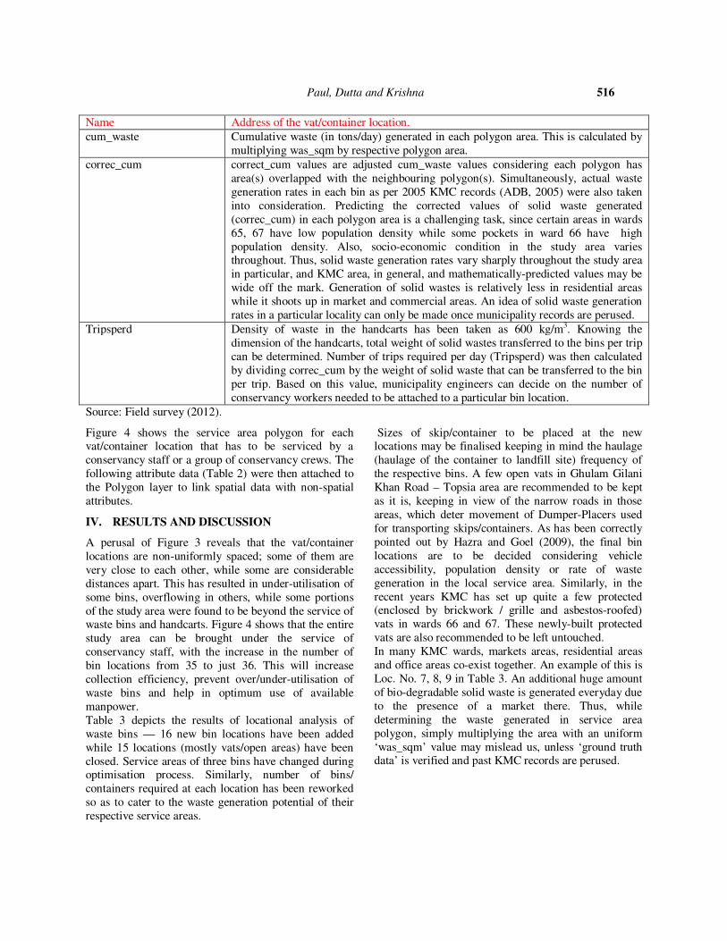
Table 2. Attribute data generated in attribute table after analysing and optimising bin locations.
Name Address of the vat/container location.
Area_sqm ArcGIS calculates the areas of each service area polygon.
Ward_no Ward no. of each container location is input.
was_sqm Waste generated per day in KMC area at present (year 2014) is assumed as 0.491 kg
/capita/ day (Paul et al., 2014).
Population of wards 65, 66, 67 are 80098, 70179, 54380 respectively (Census, 2001)
and area of wards 65, 66, 67 are 1352051.92181 sq.m, 3398330.31364
sq.m and 1836720.48955 sq.m respectively.
From these data, waste generated (in kg) per sq.m per day (was_sqm) has been
calculated.
Paul, Dutta and Krishna 516
Source: Field survey (2012).
Figure 4 shows the service area polygon for each vat/container location that has to be serviced by a
conservancy staff or a group of conservancy crews. The
following attribute data (Table 2) were then attached to
the Polygon layer to link spatial data with non-spatial
attributes.
IV. RESULTS AND DISCUSSION
A perusal of Figure 3 reveals that the vat/container
locations are non-uniformly spaced; some of them are
very close to each other, while some are considerable
distances apart. This has resulted in under-utilisation of
some bins, overflowing in others, while some portions
of the study area were found to be beyond the service of waste bins and handcarts. Figure 4 shows that the entire
study area can be brought under the service of
conservancy staff, with the increase in the number of
bin locations from 35 to just 36. This will increase
collection efficiency, prevent over/under-utilisation of
waste bins and help in optimum use of available
manpower.
Table 3 depicts the results of locational analysis of
waste bins — 16 new bin locations have been added
while 15 locations (mostly vats/open areas) have been
closed. Service areas of three bins have changed during optimisation process. Similarly, number of bins/
containers required at each location has been reworked
so as to cater to the waste generation potential of their
respective service areas.
Sizes of skip/container to be placed at the new locations may be finalised keeping in mind the haulage
(haulage of the container to landfill site) frequency of
the respective bins. A few open vats in Ghulam Gilani
Khan Road – Topsia area are recommended to be kept
as it is, keeping in view of the narrow roads in those
areas, which deter movement of Dumper-Placers used
for transporting skips/containers. As has been correctly
pointed out by Hazra and Goel (2009), the final bin
locations are to be decided considering vehicle
accessibility, population density or rate of waste
generation in the local service area. Similarly, in the
recent years KMC has set up quite a few protected (enclosed by brickwork / grille and asbestos-roofed)
vats in wards 66 and 67. These newly-built protected
vats are also recommended to be left untouched.
In many KMC wards, markets areas, residential areas
and office areas co-exist together. An example of this is
Loc. No. 7, 8, 9 in Table 3. An additional huge amount
of bio-degradable solid waste is generated everyday due
to the presence of a market there. Thus, while
determining the waste generated in service area
polygon, simply multiplying the area with an uniform
‘was_sqm’ value may mislead us, unless ‘ground truth data’ is verified and past KMC records are perused.
Name Address of the vat/container location.
cum_waste Cumulative waste (in tons/day) generated in each polygon area. This is calculated by
multiplying was_sqm by respective polygon area.
correc_cum correct_cum values are adjusted cum_waste values considering each polygon has
area(s) overlapped with the neighbouring polygon(s). Simultaneously, actual waste
generation rates in each bin as per 2005 KMC records (ADB, 2005) were also taken
into consideration. Predicting the corrected values of solid waste generated
(correc_cum) in each polygon area is a challenging task, since certain areas in wards
65, 67 have low population density while some pockets in ward 66 have high
population density. Also, socio-economic condition in the study area varies throughout. Thus, solid waste generation rates vary sharply throughout the study area
in particular, and KMC area, in general, and mathematically-predicted values may be
wide off the mark. Generation of solid wastes is relatively less in residential areas
while it shoots up in market and commercial areas. An idea of solid waste generation
rates in a particular locality can only be made once municipality records are perused.
Tripsperd Density of waste in the handcarts has been taken as 600 kg/m3. Knowing the
dimension of the handcarts, total weight of solid wastes transferred to the bins per trip
can be determined. Number of trips required per day (Tripsperd) was then calculated
by dividing correc_cum by the weight of solid waste that can be transferred to the bin
per trip. Based on this value, municipality engineers can decide on the number of
conservancy workers needed to be attached to a particular bin location.

Paul, Dutta and Krishna 517
Table 3: Bin locations before and after optimization.
LOC. NO.
NAME AREA_SQM (old)
AREA_SQM (revised)
WAS_SQMc kg sqm-1d-1
CUM_WASTE (tons d-1)
CORREC_CUM (tons d-1)
EXISTING CAPACITY RECOMMENDATIONS ASSUMING DAILY COLLECTION OF WASTE
1 29A, Palm Avenue 518885.594 518885.594 0.029 15 3.00000 2MT capacity skip/container; 01 no. 02 skips to be placed
2 64, Bondel Road (Dey’s Medical) 454316.625 454316.625 0.029 0.5X(13.175)= 6.5875
2.19000 2MT capacity skip/container; 01 no.
Total 03 skips to be placed.
3 64, Bondel Road (Dey’s Medical) 454316.531 454316.531 0.029 0.5X(13.175)= 6.5875
2.19000 2MT capacity skip/container; 01 no.
4 Tiljala Road, Near Hindustan Engineering Industries & VVF
477620.906 477620.906 0.029 13.85 3.00000 2MT capacity skip/container; 01 no. 02 skips to be placed
5 Rifle Range Road & Dr. Biresh Guha Street Crossing
524310.188 524310.188 0.029 15.2 3.04000 2MT capacity skip/container; 01 no. 02 skips to be placed
6 Graphic Pick 16 (88°22'41.215"E 22°32'11.886"N )
396588.281 0.029 11.5 3.00000 New container location proposed 02 skips to be placed
7 CIT Market 225375.703 225375.703 0.0145 3.28 2.00000 2MT capacity skip/container; 01 no.
Total 03 skips to be placed
8 CIT Market Market Waste 2.00000 2MT capacity skip/container; 01 no.
9 CIT Market 2.00000 2MT capacity skip/container; 01 no.
10 Opposite Kasba Utsav Maidan 438057.906 438057.906 0.0145 0.5 X(6.351)=3.1755
1.59000 2MT capacity skip/container; 01 no.
Total 02 skips to be placed
11 Opposite Kasba Utsav Maidan 502278.781 502278.781 0.0145 0.5X(7.28)= 3.64 1.82000 2MT capacity skip/container; 01 no.
12 Ward 67 Office, Swinhoe Lane 5062866.49 394726.375 0.0145 5.723 1.43000 2MT capacity skip/container; 01 no. 01 skip to be placed
13 G S Bose Road Lalkuthi Water Tank 425223.219 425223.219 0.0145 6.616 4.00000 2MT capacity skip/container; 01
no. 02 skips to be placed
14 Swinhoe Lane Bustee 567278.875 567278.875 0.0145 8.225 2.50000 Open Vat (protected) 5 MT Open Vat (protected) 5MT
15 Tiljala Road 368262.969 368262.969 0.029 10.68 3.56000 2MT capacity skip/container; 01 no. 02 skips to be placed
16 16, East Topsia Road 384507.875 384507.875 0.01 3.84 0.96000 2MT capacity skip/container; 01
no. 01 skip to be placed
17 10, Topsia Road East 442426.750 442426.750 0.01 4.4 2.00000 2MT capacity skip/container; 01 no. 01 skip to be placed

Paul, Dutta and Krishna 518
LOC. NO.
NAME AREA_SQM (old)
AREA_SQM (revised)
WAS_SQMc kg sqm-1d-1
CUM_WASTE (tons d-1)
CORREC_CUM (tons d-1)
EXISTING CAPACITY RECOMMENDATIONS ASSUMING DAILY COLLECTION OF
WASTE
18 42A Bus Stand, Opposite SBI 471021.12 494794.406 0.01 4.947 1.00000 2MT capacity skip/container; 01 no. 01 skip to be placed
19 138A, Picnic Garden Road (Siddhivinayak Timber Works)
445124.063 445124.063 0.01 4.451 1.48000 Open Vat (protected) 5 MT Open Vat (protected) 5MT
20 Graphic Pick 1 (88° 22'1.34" E, 22°
32"16.16"N)
550446.188 0.029 15.96 3.99000 New container location proposed
02 skips to be placed
21 Graphic Pick 2 (88° 22' 2.977" E, 22° 31" 52.972"N)
459797.125 0.029 13.33 3.33000 New container location proposed 02 skips to be placed
22 Graphic Pick 3 (88° 22' 50.63" E, 22° 32" 2.551"N)
490245.313 0.01 4.902 2.45000 New container location proposed 02 skips to be placed
23 Graphic Pick 4 (88° 23' 21.374"E, 22°
31" 33.534"N)
471207.875 0.0145 6.832 1.70800 New container location proposed
01 skip to be placed
24 Graphic Pick 5 (88° 23' 9.439"E, 22° 31"23.169"N)
334845.063 0.0145 4.855 1.21375 New container location proposed 01 skip to be placed
25 Graphic Pick 6 (88° 23' 7.889"E, 22° 31"41.536"N)
488238.344 0.01 4.88 0.70000 New container location proposed 01 skip to be placed
26 Graphic Pick 7 (88° 23' 5.571"E, 22° 31"52.651"N)
390832.719 0.01 3.908 0.55000 New container location proposed 01 skip to be placed
27 Graphic Pick 8 (88° 23' 16.286"E, 22° 32" 0.317"N)
406123.406 0.01 4.06 2.00000 New container location proposed 01 skip to be placed
28 Graphic Pick 9 (88° 23' 45.293"E, 22° 31"54.168"N)
537114.688 0.01 5.371 1.07420 New container location proposed 01 skip to be placed
29 Graphic Pick 10 (88° 23' 26.9"E, 22° 32"31.002"N)
376195.563 0.01 3.76 0.94000 New container location proposed 01 skip to be placed
30 Graphic Pick 11 (88° 23' 47.729"E, 22° 32"35.53"N)
517265.344 0.01 5.17 1.72000 New container location proposed 01 skip to be placed
31 Graphic Pick 12 (88° 23' 13.292"E, 22° 32"45.199"N)
417136.000 0.01 4.17 2.00000 New container location proposed 01 skip to be placed
32 Graphic Pick 13 (88° 23' 37.642"E, 22° 32"16.334"N)
239101.516 0.01 2.39 2.00000 New container location proposed 01 skip to be placed
33 Graphic Pick 14 (88° 24' 4.846"E, 22° 32"1.5"N)
324454.406 0.01 3.244 1.08130 New container location proposed 01 skip to be placed
34 Graphic Pick 15 (88° 23' 54.752"E, 22° 32"20.15"N)
413249.969 0.01 4.13 1.37600 New container location proposed 01 skip to be placed
35 Opposite 10/A, Topsia Road (S) 488407.51 427214.500 0.01 4.27 2.13500 Open Vat 1.5 MT 02 skips to be placed
36 38, Ghulam Gilani Khan Road 159447.250 159447.250 0.01 1.59 0.75000 Open Area; narrow road Open Vat

Paul, Dutta and Krishna 519
LOC.
NO.
NAME AREA_SQM
(old)
AREA_SQM
(revised)
WAS_SQMc
kg sqm-1d-1
CUM_WASTE
(tons d-1)
CORREC_CUM
(tons d-1)
EXISTING CAPACITY RECOMMENDATIONS
ASSUMING DAILY COLLECTION OF WASTE
37 Lumbini Park Mental Hospital 542169.44 2MT capacity skip/container; 01 no. To be closed
38 32, Shamsul Huda Road (Near Ward 65 Office)
471219.67 Open Vat To be closed
39 32, Shamsul Huda Road 471219.67 Open Vat To be closed
40 4D, Sapgachi 1st Lane 480973.15 Open Vat To be closed
41 2, Kustia Road 481760.92 Open Vat To be closed
42 21, Topsia Road 326114.65 Open Vat To be closed
43 35, Topsia Road 314015.27 Open Vat To be closed
44 26, Topsia Road 346079.99 Open Vat To be closed
45 4A, Ghulam Jilani Khan Road 396476.56 Open Area To be closed
46 56, Topsia Road (S) Near Dargah Iftakhariya
418017.34 Open Area To be closed
47 35/A, Topsia Road (S) 357323.06 Open Area To be closed
48 59, Gulam Jilani Khan Road 390971.64 Open Area To be closed
49 Tiljala Road, Near KMC Pumping Station
377335.82 Open Vat To be closed
50 Tiljala Road 484149.97 Open Vat To be closed
51 Opposite 31, Tiljala Masjid Bari Lane 459554.01 2MT capacity skip/container; 01 no. To be closed
c WAS_SQM is calculated based on AREA_SQM(revised) value

Paul, Dutta and Krishna 520
REFERENCES
[1]. ADB (Asian Development Bank) (2005). Kolkata
Environmental Improvement Project Report. Report,
Kolkata Municipal Corporation, Kolkata, India.
[2]. Ahmed SM (2006). Using GIS in Solid Waste
Management Planning A case study for Aurangbad,
India. Master’s Thesis, Linköpings University, Sweden. [3]. Chattopadhyay S, Dutta A and Ray S (2009).
Municipal solid waste management in Kolkata, India –
A review. Waste Management 29(4): 1449-1458.
[4]. CPHEEO (Central Public Health & Environmental
Engineering Organisation) 2000 Manual on Municipal
Solid Waste Management. New Delhi: Ministry of
Urban Development, Govt. of India.
[5]. Ghose MK, Dikshit AK and Sharma SK (2006). A
GIS based transportation model for solid waste disposal
— A case study on Asansol municipality. Waste
Management 26(11): 1287-1293.
[6]. Hazra T and Goel S (2009). Solid Waste Management in Kolkata, India: Practices and
Challenges. Waste Management 29(1): 470-478.
[7]. Illeperuma IAKS and Samarakoon L (2010).
Locating Bins using GIS. International Journal of
Engineering & Technology, 10(02): 97- 110.
[8]. Kolkata Environment Improvement Project (KEIP)
(2003). Master Plan on Solid Waste Management.
Report, Kolkata Municipal Corporation, Kolkata, India.
[9]. Kyessi A and Mwakalinga V (2009). GIS
Application in Coordinating Solid Waste Collection:
The Case of Sinza Neighbourhood in Kinondoni
Municipality, Dar es Salaam City, Tanzania. In: Report of Federation Internationale des Geometres. (FIG)
Working Week 2009. Surveyors Key Role in
Accelerated Development, Eilat, Israel, 3-8 May 2009,
pp.1-19. FIG Publication.
[10]. Paul K, Dutta A and Krishna AP (2014). A
Comprehensive Study on Landfill Site Selection for
Kolkata City, India. Journal of the Air & Waste
Management Association 64(7): 846–861. doi:
10.1080/10962247.2014.896834
[11]. Vijay R, Gautam A, Kalamdhad A, Gupta A and
Devotta S (2008). GIS-based locational analysis of
collection bins in municipal solid waste management systems. Journal of Environmental Engineering and
Science, 7(1): 39–43.