1

University of L’AquilaCenter of Excellence DEWS

Poggio di Roio 67040 L’Aquila, Italyhttp://www.diel.univaq.it/dews

Locating ZigBee Nodes Using the TI’s CC2431 Location Engine: A Testbed Platform and New

Solutions for Positioning Estimation of WSNs in Dynamic Indoor Environments

Stefano Tennina, Marco Di Renzo��Fabio Graziosi, Fortunato Santucci

������������ ������ � �

� ������ ������ ������� �����������

� ��������������� ��� �

��������� ��� ������ ��

! �" #$��� ���%���������&� � � '��� ����� (���)*��+##$

2

Outline

• Positioning as a Service in WSNs• Recursive Methods• Optimization Algorithms• Network Scenarios and Simulation Results• CC2431 Platform in a Dynamic Environment• Conclusions and further issues

3

Positioning� ��� �� ��� ������� �� �� � ���� ������� ���� ��������� ��� ���� ������� ������������ ����� �� ��� ������������������������������������������ ������������������������

R1

R3

R2

MS

BS

BS

BS

Known Location (anchor)

Unknown Location (node)

4

Positioning

• Main assumptions in a WSN:– Devices with limited capabilities (energy,

computation, transmission range)– No centralization of computation activity– Cooperative ranging between pairs of nodes– Few anchor (with known position) nodes

• Performance indexes:– Accuracy

– Convergence Time

5

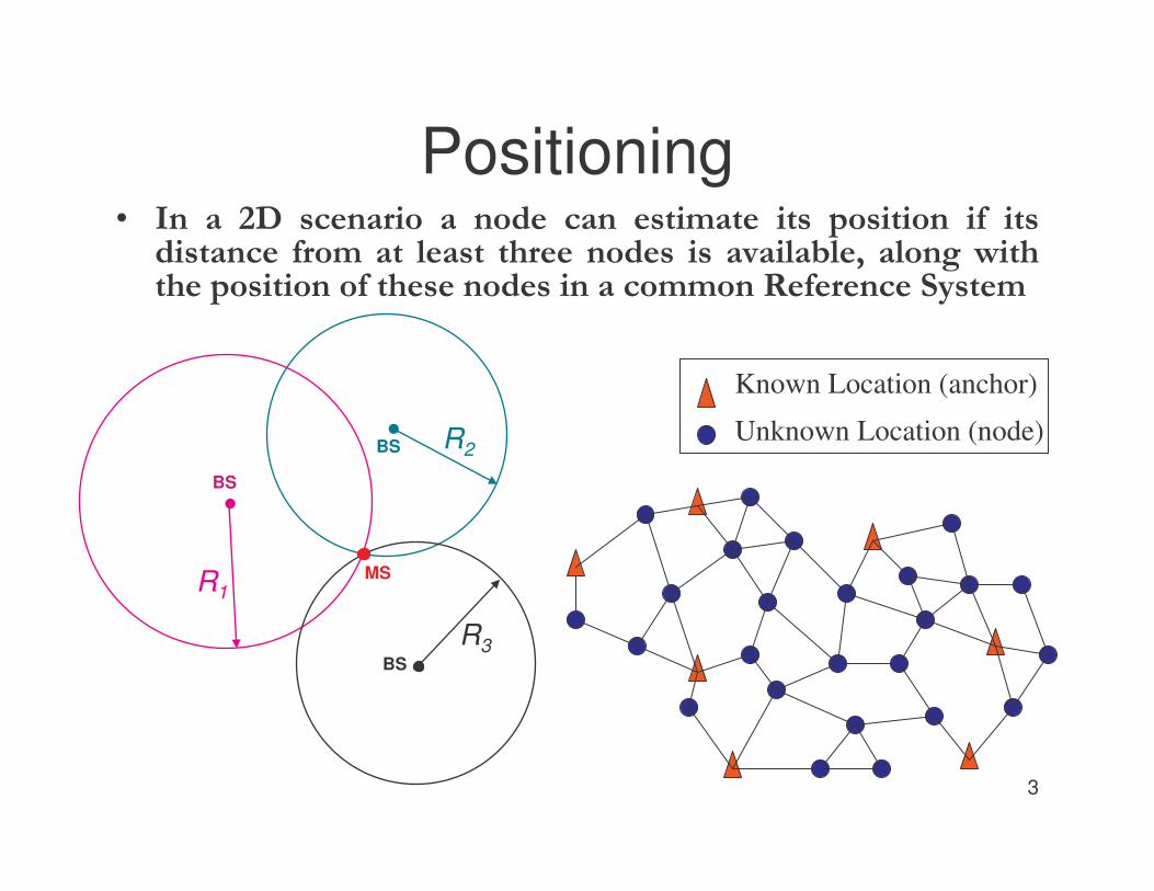
PBD Approach to Embedded System Design

• Platform Based Design is an actual research line at UC Berkeley

• This methodology consists in the definition of Platform as a library of resources defining an abstraction layer which

– hides unnecessary details – exposes only relevant parameters and functions

• Neither Top-Down nor Bottom-Up, rather Meet-in-the-Middle Approach between the requirements propagation and the performance evaluation

Upper Platform

Lower Platform

Requirements Performance

6

Sensor Network Service Platform

• PBD enables the definition of a node architecture, composed by:– An Application Interface

which:• exposes a set of relevant

services and• hides lower networking

details.– A middleware layer of

services, which implements the exposed functionalities by resorting to the underlying protocol stack entities

Service Layer

Sen

sor N

etw

ork

Ser

vice

s P

latfo

rm

Que

ry/C

omm

and

Tim

e/Sy

ncNa

min

g

Loca

tion

NodeProtocol Stack

Application

Application Interface

Environment monitoring & control

7

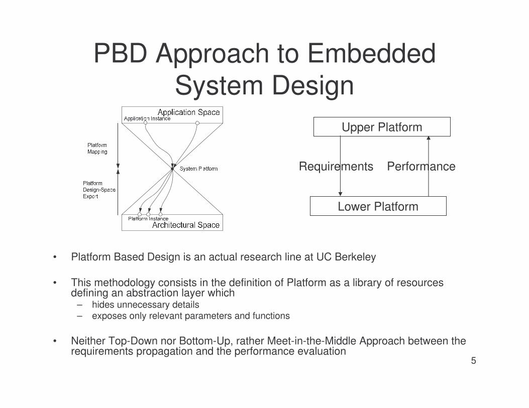
Platform Stack

Application Interface

Application Specification

Locationing Func. & Par.

Location Algorithm interface

Location Func. Struct. & Par.

Location Alg. Struct. & Par.

Location Support interface

Ranging Func. Struct. & Par.

Ranging/Comm. Func. Struct. & Par.

Application

Functional Decomposition

Location Design

Ranging/Data-link Co-Design

Physical Layer Design

Ranging/Comm interface

Ranging/Comm. Func. Struct. & Par.

Physical Struct. & Par.

At each platform, issues with an increasing level of details are addressed

8

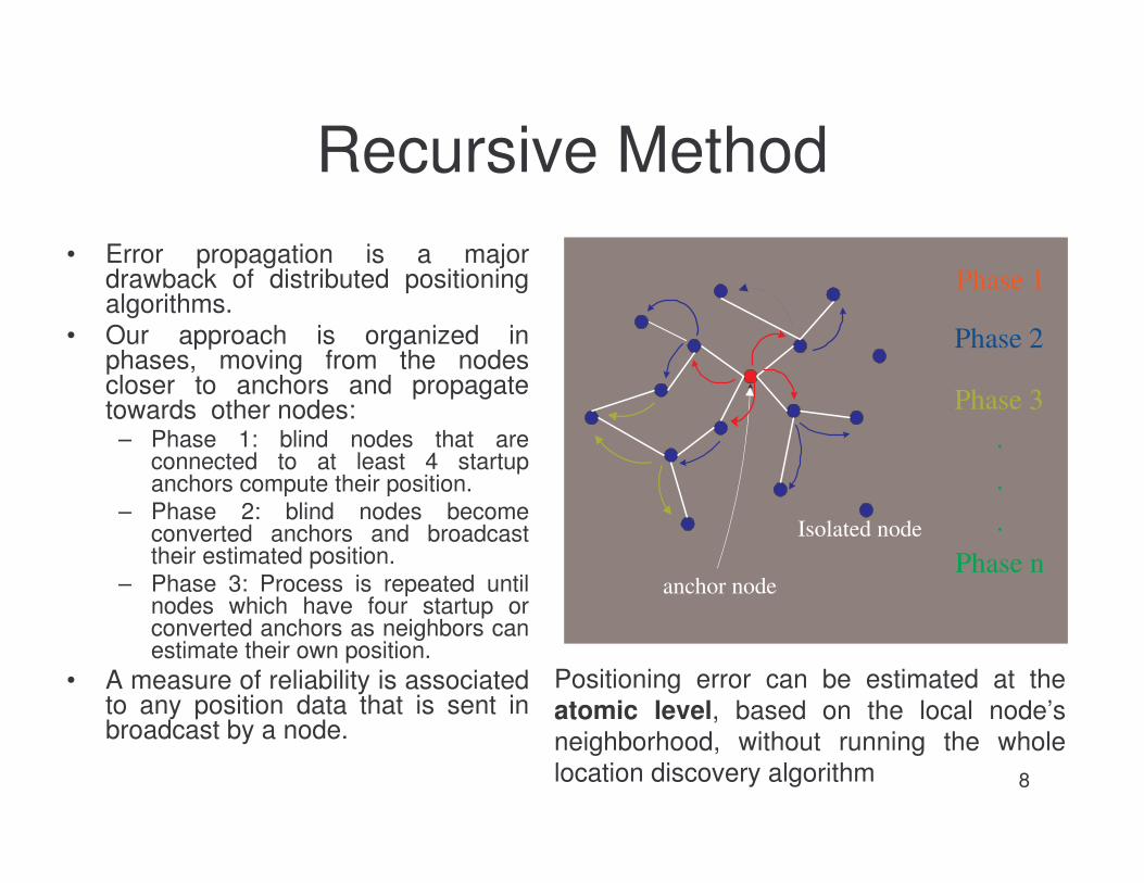
Recursive Method• Error propagation is a major

drawback of distributed positioning algorithms.

• Our approach is organized in phases, moving from the nodes closer to anchors and propagate towards other nodes:

– Phase 1: blind nodes that are connected to at least 4 startup anchors compute their position.

– Phase 2: blind nodes become converted anchors and broadcast their estimated position.

– Phase 3: Process is repeated until nodes which have four startup or converted anchors as neighbors can estimate their own position.

• A measure of reliability is associated to any position data that is sent in broadcast by a node.

Isolated node

anchor node

Phase 1

Phase 2

Phase 3...

Phase n

Positioning error can be estimated at the atomic level, based on the local node’s neighborhood, without running the whole location discovery algorithm

9

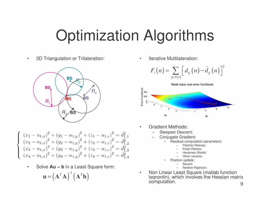
Optimization Algorithms• 3D Triangulation or Trilateration:

• Solve Au = b in a Least Square form:

• Iterative Multilateration:

• Gradient Methods:– Steepest Descent;– Conjugate Gradient:

• Residual computation parameters:– Fletcher-Reeves;– Polak-Ribiére;– Hestenes–Stiefel;– Other variants;

• Position update:– Secant;– Newton-Raphson;

• Non Linear Least Square (matlab function lsqnonlin), which involves the Hessian matrix computation.

( ) ( ) ( )( )

2

i ij ijj N i

F n d n d n∈

� �= −� ���

R1

R3

R2

MS

BS

BS

BS

R4

BS

( ) ( )-1T T=u A A A b

10

Position RefinementAlgorithm

( ) ( ) ( )( )

2

i ij ijj N i

F n d n d n∈

� �= −� ���

Update algorithm for a node i

Require: , where al = AccuracyLevel

Ensure: a new estimation of

1: for each node i do

2:

3:

4: , rp = RangingPenalty

5: Update estimation and accuracy level

Steepest descent

algorithm

( ), ,i

x y al( ), , , ( )

jx y al j N i∈

Error function

( ) ( ) ( )

( ) ( ) ( )

11

2

11

2

ii i

i

ii i

i

Fx n x n n

x

Fy n y n n

y

µ

µ

� � �∂+ = + ⋅ − �∂ � �

� �∂ + = + ⋅ − � ∂� �

( ) ( )( ) ( ) ( )( )

( )2 1 iji

i jj N ii ij

d nFn x n x n

x d n∈

� �� �∂ = − ⋅ −� � � �∂ � �� � �� �

( ) ( )( ) ( ) ( )( )

( )2 1 iji

i jj N ii ij

d nFn y n y n

y d n∈

� �� �∂ = − ⋅ −� � � �∂ � �� � �� �

( )

( )

jj N i

i

al rp

alN i

∈

� �−� �

� �� �=�

11

Enhanced Steepest Descent• Steepest Descent shows good accuracy but has a slow

convergence speed.• ESD adjusts the step length �k of the line search method as

a function of the current (p(k)) and previous (p(k-1)) search directions (that is, the error function’s gradient):

• As a matter of fact, four degrees of freedom are available to simultaneously control the convergence rate and oscillatory phenomenon when approaching the final solution, without appreciably increasing the SD original complexity.

( ) ( )( )

min max

, 1

11,

k k kθγδθ θ

= ∠ −

<>

p pPhase angleLinear Increment

Multiplicative DecrementAngular Thresholds

12

MATLAB Simulation Scenario

• Four reference nodes and one blind node which may be located in one of the Th positions, with h = 1, …, 9.

• Blind sees reference nodes with an increasing angle moving from T1(bad geometry) to T9 (ideally optimal topology condition).

• Ranging error simulated as a Gaussian with mean value given by actual distance and standard deviation �R.

Source: S. Tennina, M. Di Renzo, F. Graziosi, and F. Santucci, “On the Distribution of Positioning Errors in Wireless Sensor Networks: A Simulative Comparison of Optimization Algorithms,” IEEE WCNC, Las Vegas, March - April 2008

13

ESD vs SD convergence speed

• Initial learning speed �k = 0.1;• Linear increment � = 0.1• Multiplicative decrement � = 1.75• Angular Thresholds �min = 5°and �max = 30°

• ESD significantly improves the convergence speed of SD by reaching similar accuracy levels with a considerably less number of iterations

14

Performance of the considered Optimization Algorithms

• STD ranging error �R=0.8m;• Positioning error decreases when

moving from T1 to T9 due to network topology;

• Triangulation algorithm (INV) provides the worst performances in terms of accuracy;

• ESD provides the same accuracy as the SD and Non-linear Least Square (NLS), but reaching the final solution faster;

• ESD performs as well as CG in most scenarios, but outperforms CG when topologies are more prone to ambiguities.

CG1 = Fletcher–Reeves Polak–Ribiére with secant methodCG2 = Hestenes–Stiefel with secant method

Source: S. Tennina, M. Di Renzo, F. Graziosi, and F. Santucci, “On the Distribution of Positioning Errors in Wireless Sensor Networks: A Simulative Comparison of Optimization Algorithms,” IEEE WCNC, Las Vegas, March - April 2008

CC2431 Platform

15

• Distributed bidimensional location finder system

• Implements the Motorola’s IEEE 802.15.4 standard–based radio–location solution exploiting a maximum likelihood estimation algorithm.

• RSSI–based ranging strategy according to which the distance information between a pair of transmit and receive nodes is extracted from the received power level.

• 3 to 16 anchor nodes• 3m to 5m position estimation accuracy• 50us to 13ms time to estimate the

position with minimum CPU usage

Network Setup• 9 anchor nodes placed on

the edge of the laboratory on the top of wood supports (1.15m), which send beacons in a scheduled fashion.

• One blind node running the Location Engine (LE) for positioning estimation.

• 1 sniffer node for recording on a PC the messages exchanged by nodes and view the network topology.

16

17

CC2431 Static RSSI Calibration• Received Signal Strength

Indicator (RSSI) imposes a characterization of the propagation environment.

• Parameters A and n can be estimated empirically by collecting RSSI data (thus path loss data) for which the distances between the transmitting and receiving devices are known.

• A least-squares best-fit line is used to glean the specific values of A and n for the environment in which the data were measured:– A is the y-intercept of the line,

and– n is the slope of that line.

10( ) 10RSSI A

nd f RSSI−

= =

CC2431 Dynamic RSSI Calibration

• In this kind of scenario we can count on several anchors present in the network

• These anchors are in the neighborhood of each other• Anchor nodes:

– know their positions and thus the reciprocal distances– are transmitting in a scheduled way (e.g. anchor i waits for

transmission of anchor i-1 before it transmits its beacon)– estimate locally the path loss parameters by a linear fitting

of couples (distance, RSS) values and send their beacon with these estimations

• Blind node receives beacons from anchors and assumes as path loss parameters an average of those estimated by the anchors

18

A Dynamic Environment• During the EECI Lab’s opening ceremony on March, 27, 2008

we have conducted our experiment for evaluating the LE, when propagation characteristics of the radio channel have changed appreciably, due to people’s movement

• Four phases can be considered during the kick-off meeting:– Phase 1 is characterized by a progressive increase of the

number of people inside the room.– Phase 2 is characterized by several people (staying either

seated or stand) inside the room.– Phase 3 is characterized by the vast majority of people staying

stand and leaving the conference room.– Phase 4 when no people were in the room, thus giving a virtually

static indoor scenario with almost fixed propagation characteristics.

19

Results

20High fluctuations of the estimated parameters in dynamic phases (1-3), while almost constant in the static phase (4)

Results

21

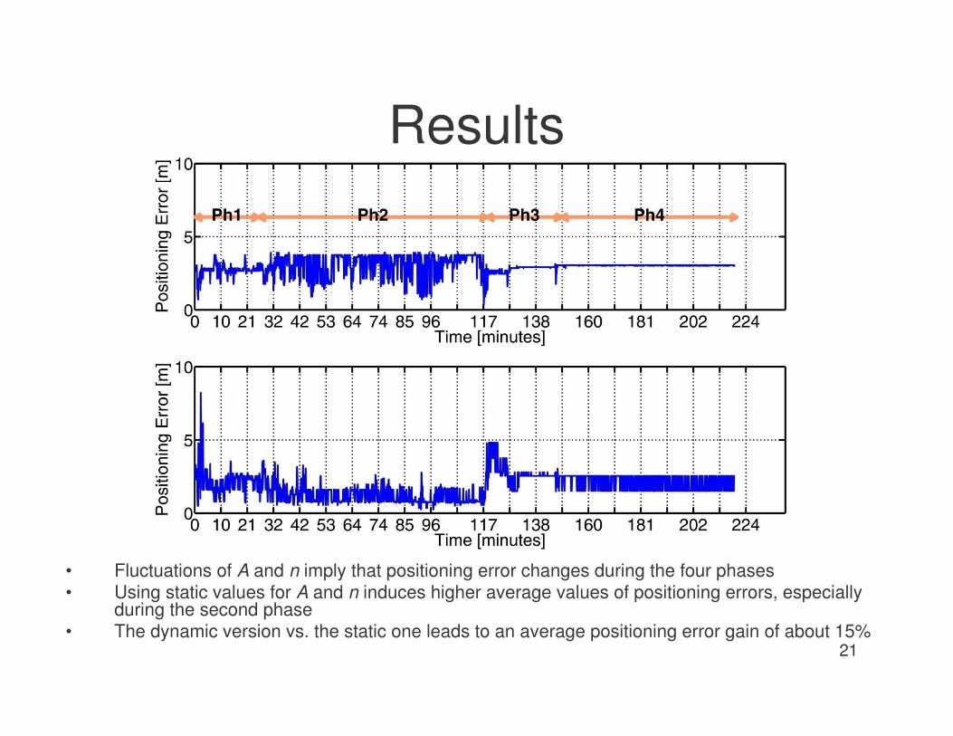
• Fluctuations of A and n imply that positioning error changes during the four phases• Using static values for A and n induces higher average values of positioning errors, especially

during the second phase• The dynamic version vs. the static one leads to an average positioning error gain of about 15%

Results

Phase Static Calibration

Dynamic Calibration

Dynamic Calibration plus ESD Refinement

Ph1 2.69m 2.20m 2.00m

Ph2 3.04m 1.22m 1.03m

Ph3 2.77m 2.72m 1.93m

Ph4 3.04m 2.11m 1.28m

• Average positioning error decreases significantly in all phases when propagation parameters are dynamically estimated.

• Adopting an ESD refinement further improves performance

22

23

Conclusions and further issues

• Ongoing and future works include:– Evaluation of the impact of the number

of anchor nodes on the performance of the proposed solution.

– Analysis of power consumptions related to the continuous training.

– Implementation of an ESD-based location engine as a true PBD network service, for supporting realistic control and monitoring applications.

• An enhanced version of the Steepest Descent algorithm has been proposed and we shown that in some scenarios it may outperform the other algorithms, while maintaining a low complexity.

• A simple solution has been proposed to counteract the effect of outdated estimation of the propagation environment in the RSSI-based ranging technique.

24

Reference

� � �,�� �� ������" ������

������������ ������ � �

� ������ ������ ������� �����������

� ��������������� ��� �

��������� ��� ������ ��

http://www.diel.univaq.it/dews

BACKUP

25

LE Dynamic vs. ESD

26

Number of Iterations ESD

27

Algorithm Details and Timing• Anchor A1 broadcasts beacons periodically every 800ms.• Anchors Ai (i = 2,..,9) wait for i-1 transmission:

– Extract RSSI and Anchor position;– Compute distance;– Estimate A and n parameters;– Broadcast its position and estimations;– Every 100 beacons of A1, it resets the average RSSI values to avoid drift in the

computation.• Blind node waits for anchor packets:

– Extracts RSSI, A, n and position of the anchor;– When at least 10 packets are received from each anchor, estimates distance moving from

the average RSSI values from each anchor and the averages of A and n;– Estimates its position passing values to Location Engine;– Sends its estimation and the used RSSIs, A and n values to the sniffer node (PC)– Every 100 beacons of A1, it resets the average the average RSSI values to avoid drift in the

computation.• If no packet loss:

– Every 8s blind node estimates and sends its position;– Every 800s blind node resets the average RSSI values from each anchor.

• No deadlock is possible in the anchors transmission chain, because A1 doesn’t wait for any other transmission.

28