Locating Velocity Changes in Elastic Media with Coda Wave

Locating Velocity Changes in Elastic Media with CodaWave Interferometry

Roel Snieder(1), Alejandro Duran(2), and Anne Obermann(2)

(1) Center for Wave Phenomena, Colorado School of Mines, Golden CO 80401, [email protected](2) Swiss Seismological Service, ETH Zurich

ABSTRACTIn coda wave interferometry one uses the long wave paths of coda waves todetect minute changes in the velocity. When the relative velocity perturbationis constant in space, it is related to the travel time change δt by δv/v = −δt/t.But when the velocity change depends on space, the relation between themeasured travel time change and the velocity change is more complicated. Weshow that in that case the estimation of velocity change can be formulatedas a standard linear inverse problem. The sensitivity kernel that relates thetravel time change to the velocity depends on the energy density of the codawaves in space. We derive these kernels for (1) diffusive acoustic waves, (2)acoustic waves that obey radiative transfer, and (3) diffusive elastic waves, andillustrate the theory with numerical examples for acoustic and elastic waves.

1 INTRODUCTION

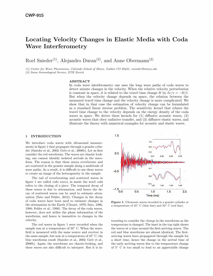
We introduce coda waves with ultrasound measure-ments in figure 1 that propagate through a granite cylin-der (Snieder et al., 2002; Gret et al., 2006b). Let us firstconsider the red waveforms. The waves are chaotic look-ing, one cannot identify isolated arrivals in the wave-form. The reason is that these waves reverberate andare scattered in the granite sample along a multitude ofwave paths. As a result, it is difficult to use these wavesto create an image of the heterogeneity in the sample.

The tail of reverberating and scattered waves infigure 1 are called coda waves, in music the word codarefers to the closing of a piece. The temporal decay ofthese waves is due to attenuation, and hence the de-cay of scattered waves can be used to estimate atten-uation (Sato and Fehler, 2012). Changes in the decayof coda waves have been used to estimate changes inthe attenuation in the Earth (Chouet, 1979; Sato, 1986,1988; Fehler et al., 1998). The decay of the coda waves,however, does not utilize the phase information of thewaveforms, and hence is insensitive to changes in thevelocity.

The red waves in figure 1 were recorded when thesample was at a temperature of 50◦ C. When the wave-field is measured with the same source and receiver inthe same sample, but now at a temperature of 45◦ C, theblue waveforms result (Snieder et al., 2002; Gret et al.,2006b). Again, the waveforms are chaotic-looking, andthese waves are also difficult to interpret. But it is in-

Figure 1. Ultrasonic waves recorded in a granite cylinder ata temperature of 45◦ C (blue line) and 50◦ C (red line).

teresting to consider the change in the waveforms as thetemperature is changed. The inset in the top right showsthe waves at a time around the first-arriving waves. Thered and blue waveforms are almost identical. The first-arriving waves have propagated through the sample fora short time, hence the change in the arrival time ofthe early arriving waves due to the temperature changeof 5◦ C is too small to lead to an appreciable change

CWP-915CWP-915

2 Roel Snieder, Alejandro Duran, and Anne Obermann

in these early arriving waves. A blowup of the later-arriving waves in a time window around 1.54 s is shownin the lower right panel of figure 1. For these later-arriving waves the red waves are a time-shifted versionof the blue waves. The later-arriving waves have spentmore time propagating through the sample, hence theyare more sensitive to the velocity change caused by the5◦ C change in temperature.

Since the coda waves have spent a longer time prop-agating through the medium than the direct waves, thecoda waves are more sensitive to changes in the velocitythan the direct wave, which makes coda waves useful fordetecting small time-lapse changes in the velocity. Thisconcept was originally proposed and applied to earth-quake doublets (Poupinet et al., 1984) and ultrasounddata (Roberts et al., 1992). As shown in the bottom-right inset of figure 1, a velocity change correspondsto a change in the arrival time of time-windowed codawaves. That change in arrival time can be measuredusing a cross-correlation (Snieder et al., 2002; Snieder,2006), which essentially is an interferometric measure-ment. For this reason the extraction of changes in mediafrom changes in recorded coda waves has been calledcoda wave interferometry. An alternative, and more ro-bust, way to extract the velocity change is the stretchingmethod where one stretches one seismogram to matchthe other seismogram (Sens-Schonfelder and Wegler,2006; Hadziioannou et al., 2009).

Coda wave interferometry has been applied to alarge number of problems that include co-seismic andpostseismic changes in seismic velocity (Schaff andBeroza, 2004; Brenguier et al., 2008; Wegler et al., 2009;Nakata and Snieder, 2011; Hobiger et al., 2012; Takagiet al., 2012; Obermann et al., 2014; Gassenmeier et al.,2016), volcano monitoring (Nishimura et al., 2000; Ya-mawaki et al., 2004; Gret et al., 2005; Brenguier et al.,2011), monitoring changes in the near surface (Sens-Schonfelder and Wegler, 2006; Mainsant et al., 2012;Larose et al., 2015a; Gassenmeier et al., 2015) and inconcrete (Tremblay et al., 2010; Zhang et al., 2016),stress changes in a mining environment (Gret et al.,2006a), geo-engineering (Hillers et al., 2015; Planeset al., 2016; Obermann et al., 2015), structural healthmonitoring (Lu and Michaels, 2005; Nakata et al., 2013;Larose et al., 2015b; Salvermoser et al., 2015), and eventhe detection of velocity changes on the moon (Sens-Schonfelder and Larose, 2008). Coda wave interferome-try has not only been used to detect velocity changes,the principle can also be used to estimate the relativedistance between repeat earthquakes (Snieder and Vrij-landt, 2005; Robinson et al., 2011, 2013), measuring themotion of scatterers in fluid flow (Cowan et al., 2000;Page et al., 2000), and detecting changes in the strengthof scatterers (Larose et al., 2010; Rossetto et al., 2011;Planes et al., 2014; Margerin et al., 2016). To a large ex-tent, these different perturbations of the wavefield canbe distinguished because they leave a different imprint

on the change in the coda waves (Snieder, 2006). Agreat boost was given to monitoring by the developmentof seismic interferometry when one retrieves the wavesthat propagate between two sensors by cross-correlatingthe noise recorded at these sensors (Lobkis and Weaver,2001; Campillo and Paul, 2003; Curtis et al., 2006;Larose et al., 2006; Snieder and Larose, 2013). Sincethe noise is always present, one can measure waves in aquasi-continuous way.

Many studies report changes in the velocity as afunction of time, but do not report where in space thevelocity is changed. When one is only interested in thetemporal behavior of the velocity, that is not needed.But there are situations where localizing the velocitychange is desirable. To what distance from an earth-quake does the velocity change? What is the depth ex-tent of the velocity change? One approach to computethe imprint of a velocity change on coda waves is to nu-merically compute waveforms before and after the ve-locity change. This approach is most useful when oneconsiders a prescribed spatial pattern of the velocitychange, such as a horizontal layer in depth or a slab(Obermann et al., 2013, 2016). This approach is, how-ever, not practical when one seeks to find a velocitychange that can have any spatial distribution. In thatcase it is useful to define sensitivity kernels that relatethe travel time change τ in a given time window to theslowness perturbation as a function of space:

τ =

∫K(r)

δs

s(r)dV . (1)

This relation has been derived for single scattered waves(Pacheco and Snieder, 2006) and for multiple scatteredwaves (Pacheco and Snieder, 2005). The sensitivity ker-nel K(r) depends on the source and receiver used, aswell as on the time window in which the travel timechange is measured. Expression (1) constitutes a linearinverse problem for the relative velocity change fromtravel time changes measured with coda wave interfer-ometry (Menke, 1984; Aster et al., 2004). Kanu andSnieder (2015b) show how one can invert equation (1)for a space-dependent slowness perturbation given setof measured changes in the arrival time of coda waves.Obermann et al. (2013, 2014) have used measurementsto locate time-lapse velocity changes related to volcaniceruptions and earthquakes.

In this work we present derivations of the kernelK(r) for a number of situations. We first consider acous-tic waves that are strongly scattered. The energy den-sity of such waves behaves as a diffusion process (vanRossum and Nieuwenhuizen, 1999; Tourin et al., 2000),which can intuitively be understood from the fact thatstrongly scattered waves follow a random walk. We alsoanalyze acoustic waves whose intensity follows the equa-tions of radiative transfer (Chandrasekhar, 1960; Ozisik,1973). For long propagation times this produces diffu-sive wave propagation, but the equations of radiativetransfer also hold for the direct wave, and scattered

Locating Velocity Changes in Elastic Media with Coda Wave Interferometry 3

waves for early times (Paasschens, 1997). Our deriva-tion is similar to recent derivations (Mayor et al., 2014;Margerin et al., 2016), but we elucidate some steps, inparticular the role of the Chapman-Kolmogorov equa-tion, in more detail. We also derive the kernels for dif-fusive elastic waves, which is important for seismolog-ical applications since the Earth is elastic. Note thatwe make no assumptions about the nature of the scat-terers, they may scatter isotropically or they may havean arbitrary radiation pattern. The information of thescatterers is encoded in the energy or specific intensityof the propagating waves, this is all the information thatis needed to compute the sensitivity kernels.

This chapter consists of the following sections. Insection 2 we derive the sensitivity kernels for stronglyscattered acoustic waves. We generalize the derivationto acoustic waves that follow radiative transfer in sec-tion 3. In section 4 we present numerical examples ofsensitivity kernels assuming diffusive wave propagation.We show an example that an inappropriate applicationof the diffusion approximation leads to erroneous ker-nels. We derive the kernels for diffuse elastic waves insection 5. The equations of radiative transfer for elas-tic waves have been developed (Ryzhik et al., 1996),but because of its complexity we refrain from derivingthe sensitivity kernels for this case. Section 6 featuresnumerical examples of the sensitivity kernels for elasticwaves. In appendices A and B we derive the Chapman-Kolmogorov equation for the diffusion equation and theequation of radiative transfer, respectively, because thistheorem plays a central role in the derivation.

2 THE TRAVEL TIME CHANGE FORDIFFUSIVE ACOUSTIC WAVES

Since the Earth is elastic, it may seem strange to treatseismological waves as acoustic waves. The coda, how-ever, is mostly comprised of shear waves (Aki andChouet, 1975). The ratio of S-wave energy density toP -wave energy density in strongly scattering 3D elasticmedia is given by

ISIP

= 2

(vPvS

)3

, (2)

where vP is the P -wave velocity and vS the S-wave ve-locity (Weaver, 1982; Tregoures and van Tiggelen, 2002;Snieder, 2002). For reasons of brevity we refer to the en-ergy density, defined as the energy per unit volume, alsoas energy. For a Poisson medium, where vP /vS =

√3,

the energy ratio (2) satisfies IS/IP ≈ 10, hence most ofthe energy resides in the shear waves. For this reason,treating the waves as scalar, acoustic, waves can be areasonable approach. In this approach one retrieves theperturbation in the shear wave velocity.

The sensitivity kernels for velocity changes forscalar waves in strongly scattering media have been de-rived by Pacheco and Snieder (2005). Their derivation

included some ad-hoc steps, notably the insertion of thevelocity change in their equation (18). We re-derive inthis section the sensitivity kernels of the travel time ofacoustic waves in strongly scattering media with thepurpose of (a) avoiding some of the ad-hoc steps in thederivation of Pacheco and Snieder (2005), and (b) pre-senting a derivation that can be extended to elastic me-dia.

In coda wave interferometry one measures the effec-tive travel time changes by cross-correlating the unper-turbed and perturbed coda waves over a time windowcentered at a central time t (Snieder, 2006). The time-windowed cross-correlation between unperturbed wavesu(t) and perturbed waves u(t) is defined as

R(ts) =

∫ t+twt−tw

u(t′)u(t′ + ts)dt′√∫ t+twt−tw

u2(t′)dt′∫ t+twt−tw

u2(t′)dt′, (3)

where the time window has center time t and width 2tw,and where ts is the time shift. The time shift ts,max forwhich this cross-correlation is a maximum is given by(Snieder, 2006)

ts,max =

∑T IT τT∑T IT

. (4)

This expression is based on the path summation wherethe scattered waves are written as a sum of the wavesthat propagate along all possible scattering trajectoriesT . The travel time change for a wave that travels alongtrajectory T is denoted by τT , and the energy den-sity of that wave is given by IT . Expression (4) thusstates that the travel time changes obtained from codawave interferometry is the energy-weighted average ofthe travel time perturbation of all waves that arrivewithin the time window used for the cross-correlation(Snieder, 2006). Since the last term in expression (4) isthe energy-weighted average of the travel time changewe denote this quantity also as an average:

〈τ〉 ≡∑

T IT τT∑T IT

. (5)

The travel time change caused by a slowness per-turbation δs for a wave propagating along trajectory Tis given by

τT =

∫T

δs dl , (6)

where the integration is along trajectory T . This is alinear approximation of the travel time change thatis based on Fermat’s theorem (Aldridge, 1994; Nolet,2008), but since the velocity changes inferred from codawave interferometry are usually a fraction of a percent(Snieder et al., 2002; Sens-Schonfelder and Wegler, 2006;Brenguier et al., 2008), this linearization can be ex-pected to work well.

Consider first the case of a constant relative slow-ness perturbation: δs/s = A = constant. The traveltime perturbation along trajectory T in equation (6)


sr

r0

dV 0t0

t � t0

Tin

Tout

Figure 2. Definition of geometric variables for the contri-bution of a velocity change in volume dV ′ at r′, a source

at s, and a receiver at r in a diffusive treatment. Only two

incoming and outgoing trajectories are shown. Incoming tra-jectories Tin and outgoing trajectories Tout can be combined

in any way to form the total trajectory from s to r throughdV ′.

is then given by τT =∫Asdl = A

∫dt = AtT , where

tT is the travel time along trajectory T . In this caseτT /tT = A = δs/s. Thus, for a constant relative slow-ness perturbation the relative travel time perturbationis equal to the relative slowness perturbation:

τTtT

=δs

s≈ −δv

v. (7)

The last identity is only true to first order in the velocityperturbation, but since the perturbation is typically lessthan 1%, the last identity is very accurate. This chapteris concerned with the situation that the relative slow-ness perturbation is not constant in space. How can thevelocity change be localized in space? Specifically, whatis the contribution of the slowness change in a volumeelement dV ′ to the observed change in arrival time ofthe coda waves in different time windows?

In the following we consider all trajectories thattravel through a volume dV ′ as shown in figure 2. Thesewaves intersect dV ′ in unknown directions, that may bedifferent for each trajectory, hence the correspondinglength of intersection dl of a trajectory with the volumedV ′ is unknown. This complication can be avoided byexpressing the line-integral (6) as a time-integral usingthat dl = s−1dt′, where s is the slowness:

τT =

∫ t

0

δs

s(rT ) dt′ , (8)

where the integration is along the path rT (t′) of trajec-tory T as a function of t′. The unperturbed travel timeis given by t, hence the time integral is limited to theinterval 0 < t′ < t taken for the waves to propagatefrom the source s to the receiver at r. Inserting thisexpression in equation (5) gives

〈τ〉 =

∑T IT

∫ t

0

δs

s(rT ) dt′∑

T IT. (9)

Expression (9) gives the change in arrival of the

coda waves in terms of the slowness perturbation alongall possible paths. We next reorder this sum over pathsto find the contribution of the slowness change in thevolume dV ′ in figure 2. As shown in that figure we con-sider incoming trajectories Tin that propagate from thesource at s to dV ′ in a time t′, and outgoing trajecto-ries Tout that propagate from dV ′ to the receive r in theremaining time t− t′. For notational simplicity we firstconsider the contribution to the energy density of allpaths that propagate through dV ′ at a fixed time t′, weindicate this quantity by

∑T through dV ′ IT . We assume

for the moment that the energy of the waves that prop-agate from the source at s through dV ′ to the receiverat r is the product of the energy of the waves that prop-agate from s to dV ′ and from dV ′ to r. We substantiatethis assumption below in expression (12), but first pro-vide a heuristic explanation. As shown in figure 2, everypath T from s to r through dV ′ consists of an incomingsegment Tin from s to dV ′ and an outgoing segment Tout

from dV ′ to r. Therefore the sum of all paths from s tor that traverse dV ′ can be written as a double sum overpaths Tin and Tout:

∑T =

∑Tin

∑Tout

. This means

that when we consider all the paths that intersect dV ′

at time t′, we can write the contribution of the energyof the paths that intersect dV ′ as∑

T through dV ′ IT (r¯, s, t)

=∑

ToutITout(r, r

′, t− t′)∑

TinITin(r′, s, t′)dV ′ ,

(10)where ITin(r′, s, t′) is the energy of the wave that prop-agates along a trajectory Tin from s to r′ in time t′. Thetotal energy of these waves in the volume dV ′ is givenby∑

TinITin(r′, s, t′)dV ′. This wave energy then propa-

gates in a time t− t′ to r, the propagation of the energyis accounted for by the term

∑Tout

ITout(r, r′, t − t′).

Denoting the total energy of the waves along all in-coming trajectories by I(r′, s, t′), and the energy of thewaves that propagate along all outgoing trajectories byI(r, r′, t−t′), the contribution to the energy of the wavesthat propagate through dV ′ is given by∑T through dV ′

IT (r, s, t) = I(r, r′, t− t′)I(r′, s, t′)dV ′ .

(11)This expression is a consequence of the Chapman-Kolmogorov theorem for diffusion that is derived in ex-pression (A9) of appendix A. Expression (11) is, how-ever, dimensionally not correct. In fact, following equa-tion (A9), it is more precise to write expression (11)as ∑T through dV ′

IT (r, s, t) = GD(r, r′, t− t′)I(r′, s, t′)dV ′ ,

(12)where GD(r, r′, t − t′) is the Green’s function for thediffuse energy that propagates from r′ to r in a time t−t′. This Green’s function satisfies the diffusion equation


for an impulsive source

∂GD(r, r′, t)

∂t−∇ · (D(r)∇GD(r, r′, t)) = δ(r− r′)δ(t) ,

(13)where D(r) is the diffusion constant of the energy den-sity.

Integrating expression (12) over dV ′ shows that theenergy density at location r is given by

I(r, s, t) =

∫GD(r, r′, t− t′)I(r′, s, t′)dV ′ . (14)

This expression states that the energy at a time t fol-lows from the energy at an arbitrary earlier time t′ ifthe diffusive Green’s function is known. Margerin et al.(2016) derive this result heuristically from Bayes’ theo-rem, which presumes that the energy can be treated asa probability. Our treatment does not invoke a prob-abilistic interpretation, but both treatments give thesame result. Applying the reasoning of section 18.4of Snieder and van Wijk (2015) to expression (13), itfollows that the Green’s function GD has dimension1/volume, hence expression (14) is dimensionally cor-rect.

Using expression (12) in the numerator of equation(9), and integrating over all volume elements dV ′ gives

〈τ〉 =

∫ ∫ t

0GD(r, r′, t− t′)I(r′, s, t′)

δs

s(r′) dt′dV ′

I(r, s, t),

(15)where we replaced the denominator of expression (9) byI(r, s, t), the energy density of the waves that propa-gate from the source at s to the receiver at r in time t.Equation (15) can also be written as

〈τ〉 =

∫K(r′)

δs

s(r′) dV ′ , (16)

with

K(r′) =

∫ t

0GD(r, r′, t− t′)I(r′, s, t′) dt′

I(r, s, t). (17)

Reciprocity applies to the diffusion equation (Morse andFeshbach, 1953a), hence GD(r, r′, t) = GD(r′, r, t), andas a result

K(r′) =

∫ t

0GD(r′, r, t− t′)I(r′, s, t′) dt′

I(r, s, t). (18)

In this expression, the properties of the source–for ex-ample an explosion or a point force, as well as thesource strength–is contained in the energies I(r′, s, t′)and I(r, s, t), because these energies depend on the wavefield, and hence on the source that excites the waves.

Equation (16) poses the determination of the ve-locity change as a standard linear inverse problem withsensitivity kernel K(r′) (Kanu and Snieder, 2015b). Bycombining measurements of the travel time change fordifferent sources, receivers, and travel times t one canestimate δs/s as a function of location. The sensitivity

kernel in expression (17) is the same as derived earlier(Pacheco and Snieder, 2005). In order to compute thiskernel, one needs to (1) compute the energy density ofthe waves that are excited by the source at s, (2) com-pute the Green’s function GD(r′, r, t) that accounts forthe diffusive energy generated by a unit source at the re-ceiver location r that propagates to r′, and (3) convolvethese energies (the time-integral in equation (17)).

Note that the kernel in equation (18) has similarproperties as the gradient computed by adjoint methodsin full waveform inversion for earthquake- and active-source data (Tarantola, 1984a,b; Tromp et al., 2005;Fichtner et al., 2006). In these adjoint methods one cancompute updates to an Earth model by convolving thefield propagated forward in time from the source withthe waveform residual propagating backward in timefrom the receivers. In expression (18) one does the same,except that one backpropagates the energy from the re-ceiver instead of the waveform residual.

There are different ways to compute the sensitiv-ity kernels. As shown in expression (18) one needs toknow the energies, hence the computation of the ker-nels reduces to the computation of the energies. Thefirst way to do this is to model the energies by solvingthe diffusion equation for the energy density. This ap-proach presumes that one knows the diffusion constantfor a given model of the random medium that generatesthe wave scattering. One also needs to ensure that atinterfaces the diffusion equation satisfies boundary con-ditions that agree with the boundary conditions of theunderlying wave propagation problem. In the presenceof a free surface–the Earth has a free surface–one alsoneeds to account for the energy carried by surface wavemodes compared to the energy of body waves. Thesecomplexities imply that using the diffusion equationis mostly practical for random media whose statisticalproperties are constant in space. Second, one can use aMonte Carlo simulation that simulates a random walkthat corresponds to a diffusive process. A third, andsimple, alternative is to numerically model the wavefieldinstead of the energy density, and to compute the en-ergy from these wavefield simulations. Since for a givenrealization of a random medium the wavefield has sta-tistical fluctuations, one may have to average the energydensity computed for several realization of the randommedium. This approach was taken by Kanu and Snieder(2015a), who show examples for scattering media whosestatistical properties are not constant in space. We showin section 4 examples of sensitivity kernels that are com-puted in this way.

3 THE TRAVEL TIME CHANGE FROMRADIATIVE TRANSFER OF ACOUSTICWAVES

Radiative transfer accounts for the distribution of en-ergy in a scattering medium as a function of space,


sr

r0

dV 0t0

t � t0

Tin

Tout

n0

n0

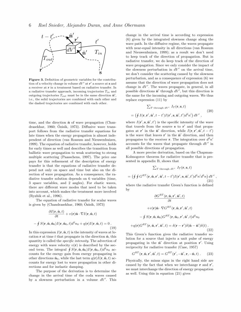
Figure 3. Definition of geometric variables for the contribu-tion of a velocity change in volume dV ′ at r′ a source at s and

a receiver at r in a treatment based on radiative transfer. In

a radiative transfer approach, incoming trajectories Tin andoutgoing trajectories Tout must be in the same direction n′,i.e., the solid trajectories are combined with each other and

the dashed trajectories are combined with each other.

time, and the direction n of wave propagation (Chan-drasekhar, 1960; Ozisik, 1973). Diffusive wave trans-port follows from the radiative transfer equations forlate times when the energy propagation is almost inde-pendent of direction (van Rossum and Nieuwenhuizen,1999). The equation of radiative transfer, however, holdsfor early times as well and describes the transition fromballistic wave propagation to weak scattering to strongmultiple scattering (Paasschens, 1997). The price onepays for this refinement of the description of energytransfer is that the equations of radiative transfer de-pend not only on space and time but also on the di-rection of wave propagation. As a consequence, the ra-diative transfer solution depends on 6 variables (time,3 space variables, and 2 angles). For elastic waves,there are different wave modes that need to be takeninto account, which makes the treatment more involved(Ryzhik et al., 1996).

The equation of radiative transfer for scalar wavesis given by (Chandrasekhar, 1960; Ozisik, 1973)

∂I(r, n, t)

∂t+ v(r)n · ∇I(r, n, t)

−∮S(r, n, n0)I(r, n0, t)d

2n0 + q(r)I(r, n, t) = 0 .(19)

In this expression I(r, n, t) is the intensity of waves at lo-cation r at time t that propagate in the direction n, thisquantity is called the specific intensity. The advection ofenergy with wave velocity v(r) is described by the sec-ond term. The integral

∮S(r, n, n0)I(r, n0, t)d

2n0 ac-counts for the energy gain from energy propagating inother directions n0, while the last term q(r)I(r, n, t) ac-counts for energy lost to wave propagation in other di-rections and for inelastic damping.

The purpose of the derivation is to determine thechange in the arrival time of the coda waves causedby a slowness perturbation in a volume dV ′. This

change in the arrival time is according to expression(6) given by the integrated slowness change along thewave path. In the diffusive regime, the waves propagatewith near-equal intensity in all directions (van Rossumand Nieuwenhuizen, 1999); as a result we don’t needto keep track of the direction of propagation. But inradiative transfer, we do keep track of the direction ofwave propagation. Since we only consider the impact ofthe slowness perturbation in dV ′ on the arrival time,we don’t consider the scattering caused by the slownessperturbation, and as a consequence of expression (6) weassume that the direction of wave propagation does notchange in dV ′. The waves propagate, in general, in allpossible directions n′ through dV ′, but this direction isthe same for the incoming and outgoing waves. We thusreplace expression (11) by∑

T through dV ′ IT (r, s, t)

=(∮I(r, r′, n′, t− t′)I(r′, s, n′, t′)d2n′

)dV ′ ,

(20)

where I(r′, s, n′, t′) is the specific intensity of the wavethat travels from the source s to r′ and that propa-gates at r′ in the n′ direction, while I(r, r′, n′, t − t′)is the wave that leaves r′ in the n′ direction, and thenpropagates to the receiver r. The integration over d2n′

accounts for the waves that propagate through dV ′ inall possible directions of propagation.

A more precise derivation, based on the Chapman-Kolmogorov theorem for radiative transfer that is pre-sented in appendix B, shows that∑

T through dV ′ IT (r, s, t)

=(∮ ∮

GRT (r, n, r′, n′, t− t′)I(r′, s, n′, t′)d2n′d2n)dV ′ ,

(21)where the radiative transfer Green’s function is definedby

∂GRT (r, n, r′, n′, t)

∂t

+v(r)n · ∇GRT (r, n, r′, n′, t)

−∮S(r, n, n0)GRT (r, n0, r

′, n′, t)d2n0

+q(r)GRT (r, n, r′, n′, t) = δ(r− r′)δ(n− n′)δ(t) .(22)

This Green’s function gives the radiative transfer so-lution for a source that injects a unit pulse of energypropagating in the n′ direction at position r′. Usingreciprocity for radiative transfer (Case, 1957)

GRT (r, n, r′, n′, t) = GRT (r′,−n′, r,−n, t) . (23)

Physically, the minus signs in the right hand side arecaused by the fact that when we interchange r and r′,we must interchange the direction of energy propagationas well. Using this in equation (21) gives


∑T through dV ′

IT =

(∮ ∮GRT (r′,−n′, r,−n, t− t′)I(r′, s, n′, t′)d2n′d2n

)dV ′ , (24)

By analogy with equation (15) we obtain for the travel time perturbation

〈τ〉 =

∫ ∫ t

0

∮ ∮GRT (r′,−n′, r′,−n, t− t′)I(r′, n′, s, t′)d2n′d2ndt′

δs

s(r′) dV ′∮

I(r, n, s, t)d2n. (25)

Writing this equation in the form of expression (1), the sensitivity kernel derived from radiative transfer is given by

K(r′) =

∫ t

0

∮ ∮GRT (r′,−n′, r′,−n, t− t′)I(r′, n′, s, t′)d2n′d2ndt′∮

I(r, n, s, t)d2n, (26)

A comparison of the radiative scattering kernel above and the kernel (18) for diffuse waves is that in radiativetransfer theory one uses waves traversing dV ′ that propagate in the same direction n′, while in the kernel (18) thereis no accounting for the direction of waves that enter dV ′ and those that leave dV ′. Physically this corresponds to thefact that diffuse waves propagate with nearly equal intensity in all directions, while in radiative transport the energypropagation may depend on direction. The radiative transfer kernel (26) stipulates that the incoming and outgoingwave in dV ′ propagate in the same direction. This corresponds to the fact that we consider the imprint of velocityvariations in dV ′ on the arrival time scattered waves, but not the scattering of waves by inhomogeneities in dV ′.

One only needs the specific intensity to compute the sensitivity kernel (26) for radiative transfer. There areseveral ways to compute the specific intensity (Wegler et al., 2006). One way to achieve this is to solve the equation ofradiative transfer directly. Since the radiative transfer equation depends on 6 variables, and it is an integro-differentialequation, this can be an involved and numerically demanding process. (Not to mention the intellectual demands.)An alternative is to use Monte-Carlo simulations where one shoots rays into the random medium that are scatteredin statistically the same way as the wave scattering (Gusev and Abubakirov, 1996; Yoshimoto, 2000; Margerin et al.,2000; Sens-Schonfelder et al., 2009). A third alternative is to first compute the wavefield numerically, and derive thespecific intensity from this wavefield. This involves locally decomposing the wavefield into the different directions ofpropagation, followed by squaring to convert the wavefield into specific intensity. The directional decomposition canbe carried out by a local Fourier transform or by local beamforming.

Since radiative transfer keeps track of the direction of wave propagation, one can, in principle, use this theoryalso to retrieve anisotropic slowness perturbations that depend on the direction of wave propagation n′ by rewritingexpressions (25) and (26) as

〈τ〉 =

∫ ∮K(r′, n′)

δs

s(r′, n′) d2n′dV ′ , (27)

and

K(r′, n′) =

∫ t

0

∮GRT (r′,−n′, r′,−n, t− t′)I(r′, n′, s, t′)d2ndt′∮

I(r, n, s, t)d2n, (28)

where K(r′, n′) measures the sensitivity to the slowness at location r′ of waves that propagates in the n′-direction.

4 AN EXAMPLE OF SENSITIVITY KERNELS AND OF THE BREAKDOWN OF DIFFUSION

To illustrate the kernels, and their limitations, we show in figure 4 the diffuse wave kernels (18) computed by Kanuand Snieder (2015a) for acoustic waves. The used model consists of a random medium that is overlain by a low-velocitylayer in the near surface and a free surface with a rough topography (Kanu and Snieder, 2015a). The source andreceiver locations are marked with S and R, respectively. The four panels are for four different lag times, that areshown the upper right hand corner of each panel. These different lag times correspond to four different regimes of wavepropagation. The kernels are computed by modeling the wavefield by finite difference simulations, and computing theenergy density from the obtained waveforms. In order to reduce fluctuations, the kernels were averaged over a fewrealizations of the random medium (Kanu and Snieder, 2015a).

The upper left panel is for a time of t = 1.4 s, which corresponds to the travel time of the ballistic, or direct,wave that propagates from source to receiver. This wave can only be influenced by velocity perturbations on the pathof the ballistic wave, and indeed the upper left panel shows a kernel that is only nonzero in the first Fresnel zone for


the ballistic wave. (A description of the Fresnel zone isgiven by Spetzler and Snieder (2004).) The wave in thistime window is in the ballistic regime.

The panel in the top right is for a slightly latertime t = 1.8 s. This time is large enough that the waveshave had the time to be scattered, but the propagationtime is so short that multiple scattering is not yet im-portant. The sensitivity kernel is nonzero mostly on anellipse with the source and receiver as focal points, al-though a weak reflected wave generated at the bottomof the near surface layer is visible just below the re-ceiver. Since this kernel corresponds to single scatteredwaves, the waves are in the single-scattering regime. At alater time t = 2.5 s, shown in the bottom left panel, thewaves have been scattered more often. As a result thesingle-scattering ellipse is filled in. The nonzero value ofthis scattering kernel within the single-scattering ellipseis caused by multiple scattering. These waves are in themultiple-scattering regime. In addition to the random in-fill of the singe-scattering ellipse by multiple scattering,a secondary ellipse is present within te single-scatteringellipse. This is due to scattered waves that reflect off thebottom off the low-velocity layer near the surface beforepropagating to the receiver.

The bottom-right panel, for travel time t = 5.0 smay be least familiar. For this late time there still is aremnant of the single-scattering ellipse near the bottom,and the speckle in the interior corresponds to multi-ple scattering. But the most conspicuous feature is thestrong value of the kernels in a horizontal band run-ning through the receiver R. The location of this hori-zontal band corresponds to the low velocity layer thatis bounded by the corrugated free surface. The strongvalue of the kernel in this low-velocity layer implies thatmost of the wave energy, and hence most of the sensitiv-ity to velocity changes, is in the low-velocity layer justbelow the free surface. For this late time, the waves arein the surface-saturated regime. Perhaps surprisingly,the near-surface layers attracts a large fraction of thewave energy, even though the source is located manywavelengths below the base of the low-velocity layer.This signifies the power of the near-surface layer to trapenergy. Simulations as shown in figure 4 give insightinto the sensitivity of the coda wave for velocity per-turbations in different regions of the model. Of particu-lar practical importance is the depth-dependence of thissensitivity.

The single-scattering ellipse in the upper rightpanel of figure 4 may seem perfectly natural, but some-thing is wrong with this figure. The problem is that thekernels are for the sensitivity of the arrival time of codawaves to a velocity perturbation; these are not the ker-nels that account for the generation of scattered waves.The sensitivity of the single-scattered waves for velocityperturbations should be distributed over the interior ofthe single-scattering ellipse, because this interior cov-ers the region of space traversed by the single-scattered

waves, and hence velocity changes in this inner regionare the cause of the changes in the arrival time of single-scattered waves.

So what went wrong? The sensitivity kernels infigure 4 are computed with the kernel (18) for diffusewaves, even though the propagation regime of the wavesin the upper right panel of figure 4 is far from diffu-sive. As sketched in figure 2, we allow in the diffusiveregime the incoming and outgoing waves at dV ′ to travelin different directions. For diffuse waves, this differencein direction of wave propagation does not matter be-cause these waves travel with near-equal intensity inall directions anyhow (van Rossum and Nieuwenhuizen,1999). But the single-scattered waves are highly direc-tional. For a volume dV ′ in the interior of the single-scattering ellipse, the situation sketched in figure 3 ismuch more realistic because for a volume element dV ′

within the single-scattering ellipse, the waves continueon a straight line to the scattering point on the scatter-ing ellipse. For this reason, the direction of propagationn must be preserved in the wave propagation withinthe single-scattering ellipse. Since this is not the casewith the used diffuse wave theory for the computationof the sensitivity kernels in figure 4, the sensitivity iserroneously confined to the single-scattering ellipse in-stead of the interior of this ellipse.

There are two ways to obtain the correct kernelsfor single-scattered waves. The first is to use the ker-nels that are designed for single-scattering (Pacheco andSnieder, 2006). The other alternative is to use the radia-tive transfer kernel (26) because these kernels stipulatethat the direction of wave propagation does not changein dV ′, as shown in figure 3. This restriction precludesthe contribution from velocity changes on the single-scattering ellipse.

5 THE TRAVEL TIME CHANGE FORDIFFUSE ELASTIC WAVES

The somewhat lengthy derivation of section 2 makesit relatively easy to determine the sensitivity kernelsfor the travel time change of the coda waves caused bychanges in the P -wave slowness sP and the S-wave slow-ness sS . The elastic displacement u can be separatedinto a curl-free part uP and a divergence-free part uS

that corresponds to the P - and S-waves, respectively(Aki and Richards, 2002): u = uP + uS . One mightthink that the energy can also be decomposed into aP -wave energy IP and an S-wave energy IS . Perhapssurprisingly, this is, strictly speaking not the case. Thiscan be seen for example by considering the contributionof the kinetic energy IKIN to the total energy, which isgiven by

IKIN =1

2ρ|uP + uS |2 =

1

2ρu2

P +1

2ρu2

S + ρ(uP · uS) ,

(29)

Locating Velocity Changes in Elastic Media with Coda Wave Interferometry 91934 C. Kanu and R. Snieder

Figure 14. Temporal and spatial evolution of the sensitivity kernel (numerical solution) showing topography-induced scattering using vertical source–receiverline.

for monitoring than using a surface-receiver array. In this case, theborehole array records more of the scattered waves generated withina given layer. This results in higher sensitivity to a change in thatlayer. Also, the borehole array, depending on its relative depth tothe free-surface, is less sensitive to waves that are scattered at ornear the free surface.

4 D I S C U S S I O N A N D C O N C LU S I O N

We propose a novel approach to compute the sensitivity kernel thatcan be used to resolve weak changes within the earth’s subsur-face or any other medium using multiply scattered waves. Theseare changes which are usually irresolvable with singly scatteredwaves. Our approach does not rely on analytical models of the scat-tered intensity such as the diffusion and radiative transfer models.To compute the sensitivity kernel, we compute the intensity fieldneeded for the kernel computation from numerically generated scat-tered wavefield. In this paper, we use finite-difference modelling forthe computation of the seismic wavefield. The numerical modellingof the scattered intensity can take advantage of various numericalmethods for seismic wavefield computation. Using our approachwe can incorporate any complexities of the scattering medium andany boundary conditions of the medium. With an appropriate a pri-ori scattering model, we can obtain a more accurate and detailedestimate of the sensitivity kernel which accurately describes the in-tensity of the scattered wave recorded by a given source–receiverpair. This numerical estimate of the sensitivity kernel potentially

allows us to resolve a more detailed localized weak changes withina scattering medium compared to changes resolved with kernelwhich depends on a global estimate of the sensitivity kernel. Ourkernel computation approach is suitable for a medium such as theearth’s subsurface where in most cases the scattering properties areheterogeneous and whose scattered intensity may not be describedanalytically.

The goal for the computation of the sensitivity kernel is to charac-terize the origin and distribution of the recorded multiply scatteredwaves use for imaging weak changes within a scattering medium. InSection 3.2.2, the relative orientation of the source–receiver array tothe scatterers within a medium affects the distribution and amountof scattered waves generated with the medium, which changes thecharacteristics of the sensitivity kernel. Imaging of weak changeswith a sensitivity kernel that does not embody the local character-istic of the scattering medium especially in statistically complexmedia might lead to errors in the retrieved velocity changes.

The caveat to the computation of the scattered intensity and inextension the sensitivity kernel for the monitoring weak changes isthe computation cost of both the scattered intensity and the corre-sponding kernel and the need for an accurate a priori model of thestatistical properties of the scattering medium. The cost of the ker-nel computation mostly depends on the traveltime of the scatteredphase for the kernel, the sum of number of sources and receivers,the number of the scattering model realizations needed, the costof the forward modelling of the scattered intensity for both thesource and receiver intensity fields, and the cost for the convolution

at Colorado School of M

ines on Novem

ber 12, 2015http://gji.oxfordjournals.org/

Dow

nloaded from

Figure 4. Sensitivity kernels for diffuse waves for a random medium with a near-surface layer as computed by Kanu and Snieder(2015a) for different lag times shown in the upper right corner of each panel. The source and receiver positions are marked by Sand R, respectively. The model has a near surface layer and rough topography of the snele surface (Kanu and Snieder, 2015a).The four panels corresponds to four different wave propagation regimes: ballistic wave propagation (top left), single scattering(top right), multiple scattering (bottom left), and the surface-saturated regime (bottom right).

where ρ is the mass density and the overdot denotes atime-derivative. The first term in the right-hand-side isthe kinetic energy of the P -waves, and the second termis the kinetic energy of the S-waves. There is, however,an additional cross-term ρ(uP · uS) that correspondsneither to the P -wave energy nor to the S-wave energy.The P and S-wave kinetic energies 1

2ρu2

P and 12ρu2

S arealways positive, but the cross-term ρ(uP · uS) can beeither positive and negative. This means that the cross-term can be eliminated by local averaging over spaceand time. Note that the presence of the cross-term is nota peculiarity of elastic waves. Consider the superpositionof two acoustic waves, u = u1 + u2. The correspondingenergy is quadratic in the wavefield and satisfies I =u21 + u2

2 + 2u1u2, hence the presence of cross-terms is ageneral consequence of superposition.

After local averaging over space and time, the wavespropagating through dV ′ can be decomposed into P andS-waves, with their energies IP and IS , respectively.The P -wave energy is for a displacement field u in anisotropic medium with Lame parameters λ and µ givenby (Morse and Feshbach, 1953b; Shapiro et al., 2000)

IP = (λ+ 2µ)(∇ · u)2 , (30)

and the S-wave energy satisfies

IS = µ|∇ × u|2 . (31)

This is twice the potential energy, but because the ki-netic and potential energy average over time is equal(Dassios, 1979), the total energy is twice the potentialenergy.�

After spatial averaging, the energy at r′ can be de-composed in contributions from P and S-waves:

I(r′, s, t′) = IP (r′, s, t′) + IS(r

′, s, t′) , (32)

where the energy for P and S-waves needs to be com-puted for the source at s, for example by prescribing

�In three dimensions there are two S-wave polarizations:uS = uS1 + uS2, and the S-wave energy is given by IS =µ|∇×uS1|2 + µ|∇×uS2|2 +2µ(∇×uS1) · (∇×uS2) . Thecross term on the right vanishes for two S-waves with orthog-onal polarization that propagate in the same direction, butis, in general, nonzero, which can be verified for the specialcase uS1 = xf(t− z/vS) and uS2 = zg(t− x/vS). The crossterm is, however, oscillatory in space, so it vanishes afterspatial averaging. This means that when one uses expression(31) for the S-wave energy and applied some spatial averag-ing, the cross-terms between the S-wave polarizations do notcontribute.


the double-couple of a moment-tensor source. A sim-ilar decomposition holds for I(r, r′, t − t′). With thisdecomposition of the energies, equation (11) for diffuseacoustic waves can for elastic waves be generalized to∑

T through dV ′ IT (r, s, t) = IP (r, r′, t− t′)IP (r′, s, t′)dV ′

+IS(r, r′, t− t′)IS(r′, s, t′)dV ′ .(33)

Note that doing so we have ignored cross-terms such asIP (r, r′, t − t′)IS(r′, s, t′) between P and S-wave ener-gies. Such cross-terms account for the mode-conversionsin dV ′, but since we aim to retrieve the kernels for thetravel time change, in contrast to the sensitivity kernelsfor the waveforms, such mode conversion are not rele-vant. This does, however, not mean there are no con-versions between P and S-waves; conversions betweenthese different wave types can occur along the pathsfrom the source to r′, and between r′ and the receiver.

Reciprocity holds for elastic waves (Aki andRichards, 2002), and it therefore also holds for the en-ergy associated with these waves, hence

IP (r, r′, t− t′) = IP (r′, r, t− t′) (34)

This energy needs to be interpreted carefully.IP (r, r′, t − t′) is the energy associated with theGreen’s function that propagates P -wave energy at r′

to the recorded component at the receiver at r. LetGDP (r′, r, t − t′) be the P -wave energy at location r′

that is generated by a unit impulsive point force at thereceiver location r in the direction of the receiver thatrecords the wavefield. This quantity corresponds to theP -wave energy associated with the elastic wave Green’sfunction Gic(r

′, r, t − t′), where i denotes the orienta-tion of this wavefield at location r′ and c the orienta-tion of the receiver at r. A similar definition holds forthe S-wave energy density Green’s function GDS . TheGreen’s function Gic is the elastic wave Green’s tensor(Aki and Richards, 2002) that should not be confusedwith Green’s function GD,P or S for the diffusive energyfor P or S-waves. In the case of a pressure receiver, GDP

is the P -wave energy at r′ generated by a unit explosivesource at r, and GDS is the corresponding S-wave en-ergy. Even though an explosive source does not generateS-waves, the S-wave energy at r′ is, in general, nonzerodue to mode conversions caused by the heterogeneity.We show numerical examples in section 6.

The rest of the derivation proceeds in the same wayas in section 2, with the difference that we multipliedexpression (11) with the relative slowness change δs/s.For elastic waves each of the terms of the right handside of equation (33) must be multiplied with the rela-tive slowness change for each wave-type. Doing so gen-eralizes equations (16) and (17) for elastic waves to

〈τ〉 =

∫KP (r′)

δsPsP

(r′) dV ′ +

∫KS(r′)

δsSsS

(r′) dV ′ ,

(35)

with

KP (r′) =

∫ t

0GDP (r′, r, t− t′)IP (r′, s, t′) dt′

I(r, s, t), (36)

and

KS(r′) =

∫ t

0GDS(r′, r, t− t′)IS(r′, s, t′) dt′

I(r, s, t). (37)

Note that in expressions (36) and (37) the energies IPand IS in the numerator are the contributions from theP and S-waves, respectively, to the energies at r′. Bycontrast, the energy in the denominator is the total en-ergy recorded of the c component of the motion at thereceiver location r, just as it is in equation (17) for scalarwaves. Since for strongly scattered elastic waves theS-wave energy dominates the P -wave energy (Weaver,1982; Snieder, 2002), the sensitivity kernel KS for per-turbations in the S-wave slowness is much larger thanthe sensitivity kernel KP for perturbations in the P -wave slowness.

6 NUMERICAL EXAMPLES

In this section we present numerical examples for thesensitivity kernels KP and KS for P and S-waves. Fol-lowing expressions (30) and (31) the kernels are com-puted by taking the divergence and the curl of thewavefield computed with the spectral element method(Specfem2D) (Tromp et al., 2008). The used two-dimensional velocity medium is a superposition of a con-stant background with P -velocity 6500 m/s, and ran-dom fluctuations that obey a von Karman distribution(Sato and Fehler, 2012) with exponent κ = 0.5. At ev-ery location the P and S-waves are scaled such thatvP (r)/vS(r) =

√3 (Poisson medium). The variance of

the velocity perturbations is 20%, and the correlationlengths are given by ax = az = 325 m, which is of theorder of the wavelength for P -waves at the used domi-nant frequency of 20 Hz. A free surface is present at thetop (z = 0), and absorbing boundaries are applied tothe sides and bottom of the computational domain. Thesimulations are described by Obermann et al. (2013),who give more details on the medium characterization.

The kernels for the P and S-waves generated by anexplosive source at location s and a hydrophone (pres-sure sensor) at r are shown in figure 5. These kernelsare averaged over 4 realizations of the random medium,this suppresses fluctuations caused by the specific real-ization used. The left panels are for a time that corre-sponds to the travel time of the ballistic P -wave. Forthis early time the P -wave sensitivity is confined tothe path of the ballistic wave from s to r. Just as infigure 4, the P -wave kernel is for a slightly later time(t = 1.75 s) most prominent on the single-scattering el-lipse. As argued in section 4, the kernel should fill theinterior of the ellipse. To a certain extent this happens,in particular near the source and receiver where the


0 5 10 15 x (km)

0

5

10

15

z (k

m)

0

1

2

3

4

5

s/m

2

10-15

0 5 10 15 x (km)

0

5

10

15

z (k

m)

0

0.2

0.4

0.6

0.8

1

s/m

2

10-11

0 5 10 15 x (km)

0

5

10

15

z (k

m)

0

0.5

1

1.5

s/m

2

10-12

0 5 10 15 x (km)

0

5

10

15

z (k

m)

0

0.2

0.4

0.6

0.8

1

s/m

2

10-10

0 5 10 15 x (km)

0

5

10

15

z (k

m)

0

0.2

0.4

0.6

0.8

1

s/m

2

10-10

0 5 10 15 x (km)

0

5

10

15

z (k

m)

0

0.2

0.4

0.6

0.8

1

s/m

2

10-10

!"#$%&'

!"""""""#

!"('

!"#$%&'

!"""""""#

!")$*&'

!"""""""#

!"('

!"""""""#

$%

$&

!")$*&'

!"""""""# !"""""""#

Figure 5. Sensitivity kernels KP (top row) and KS (bottom row) for three different lag times for an explosive source. Thetime for the left panels (t = 0.65 s) corresponds to the arrival time of the direct P -wave. Note that the used grey scales for thedifferent panels are different.

sensitivity is large (Pacheco and Snieder, 2005; Mayoret al., 2014), but the largest sensitivity is confined tothe single-scattering ellipse. This discrepancy is causedby treating the single-scattered waves as being diffuse,which is not realistic. For later time (t = 3 s) P -wavesreflected off the free surface dominate the P -wave kernelin the top right panel.

The S-wave sensitivities, as shown in the bottompanels of figure 5, are caused by P → S → P conversionsbecause the explosive source does not generate S wavesand the used receiver, a hydrophone, does not detect S-waves. For the time of the direct P -wave, the bottom leftpanel of figure 5, the S-wave sensitivity is confined tosmall regions near the source and receiver. Because thetravel is equal to the travel time for the direct P-wave,there is no possibility of the wave to propagate as anS-wave, which means that the P → S → P conversionsmust take place at almost the same location. Since thisis extremely unlikely, the S-wave sensitivity is about10,000 times smaller than the P -wave sensitivity for thisearly time.

For later times (middle and right panels in bottomrow) the S-wave kernels are nonzero, despite the factthat the explosive source does not generate shear waves.This sensitivity to the shear wave velocity is caused byP → S → P converted waves by the fluctuations inthe random medium, but for these later times the modeconversions can take place at different locations. Sincethese mode conversions occur throughout the randommedium, the sensitivity kernels for the S-waves are dis-

tributed to the interior of an egg-like region in spacecentered on the source and receiver. Note that for t = 3s, the bottom right panel of figure 5, there is a slight sen-sitivity to the shear velocity near the free surface in themiddle of the shown area. This sensitivity is caused byconversions from P -waves to surface waves to P wavesby near-surface heterogeneity.

In figure 6 we compare the wavefields and time-dependence of the sensitivity kernels for waves excitedby an explosive source (left panels) and for point forces(middle and right panels) with a direction shown in thetop panels. For both wavefields the direct P -wave isclearly visible, this P -wave is isotropic for the explo-sive source (top left), but it is modulated by the radi-ation pattern of the point force in the top middle andright panels. Note that for the point force (middle andright top-panels) there is a pronounced ballistic S-wave,which is absent for the explosive source (top-left panel)because an explosion does not generate shear waves.

The panels in the middle row of figure 6 show theP and S-wave kernels for the location r′ marked in thetop panel for times up to 40 s. Note that the time-dependence for the kernels is similar, irrespective of thesource type. For the 45◦ elastic force (middle panels),the point force radiates no S-waves towards r′, yet theS-wave kernel is nonzero, as it is for the explosive sourcein the left panels. The scattering and mode conversion isso strong that the P and S wave fields equilibrate. Thisequilibration can be seen more clearly in the bottompanels of figure 6, which show the ratio of the S-wave


!

"#

$#

!

"

##$

%##$%

!"#$%&'

("#$%&'

##$

%

&'()*%+,-./*0#1- 23) &)4%5+1.6*#1- 783) &)4%5+1.6*#1-

9

0 4 8 12 16X(km)

z(km

)

0

4

8

12

16

z(km

)

z(km

)

!"#$%&' !"#$%&'

("#$%&'

4

0 4 8 12 16X(km)

0 4 8 12 16X(km)

0

4

8

12

16

0

4

8

12

16

K S/K

P

K S/K

P

K S/K

P

Figure 6. Snapshots of the wavefields (top row), sensitivity kernels KP (r′) and KS(r′) at location r′ (middle panels), and the

ratio of these kernels at r′ (bottom panels). The examples are for a source at s and a seismometer at r as shown in the toppanels. The left column is for an explosive source, while the middle and right columns are for a point force in the direction ofthe white arrows shown in the top panels.

kernel to the P -wave kernel at location r′ for the threesource types. For t > 4 s, this ratio approaches an equi-librium value KS/KP ≈ 9.

This ratio can be explained as follows. For astrongly scattering medium in two dimensions, theequilibrium ratio of the S-wave energy to the P -waveenergy is given by IS/IP = (vP /vS)

2. Accordingto expressions (36) and (37), the P -wave kernelsdepends on the product of P -wave energies (GDP

and IP ), while the S-wave kernel depends on productof S-wave energies. This means that in equilibriumKS/KP ∝ (IS/IP )

2 = (vP /vS)4. For a Poisson medium

(vP /vS =√3), this implies that KS/KP = 9. The ratio

of the kernels in the bottom panels of figure 6 is slightlyhigher than this value. We attribute this difference tothe presence of the free surface, which through the

presence of surface waves slightly modifies the ratio ofthe P and S-energies (Weaver, 1985; Hennino et al.,2001; Margerin et al., 2009; Obermann et al., 2013,2016). The large value of this ratio implies that the codawaves are mostly influenced by the S-velocity. This iseven more pronounced in three dimensions where inequilibrium IS/IP = 2(vP /vS)

3 (Weaver, 1982), henceKS/KP = 4(vP /vS)

6 = 98 for a Poisson medium. Thenumerical examples show that in the strong scatteringregime the changes in the coda depend mostly onthe changes in the S-velocity, and that the sensitivitykernels do not depend strongly on the details of theseismic source.

Acknowledgment. We thank Christoph Sens-


Schonfelder and two anonymous reviewers for theirinsightful and constructive comments.

REFERENCES

Aki, K., and L. Chouet, 1975, Origin of coda waves:source, attenuation, and scattering effects: J. Geo-phys. Res., 80, 3322–3342.

Aki, K., and P. Richards, 2002, Quantitative seismol-ogy, second ed.: Univ. Science Books.

Aldridge, D., 1994, Linearization of the eikonal equa-tion: Geophysics, 59, 1631–1632.

Aster, R., B. Borchers, and C. Thurber, 2004, Parame-ter estimation and inverse problems: Academic Press.

Brenguier, F., M. Campillo, C. Hadziioannou, N.Shapiro, and E. Larose, 2008, Postseismic relaxationalong the San Andreas Fault at Parkfield from contin-uous seismological observations: Science, 321, 1478–1481.

Brenguier, F., D. Clarke, Y. Aoki, N. Shapiro, M.Campillo, and V. Ferrazzini, 2011, Monitoring volca-noes using seismic noise correlations: Comptes Ren-dus Geoscience, 343, 633–638.

Campillo, M., and A. Paul, 2003, Long-range correla-tions in the diffuse seismic coda: Science, 299, 547–549.

Case, K., 1957, Transfer problems and the reciprocityprinciple: Rev. Mod. Phys., 29, 651–663.

Chandrasekhar, S., 1960, Radiative transfer: Dover.Chouet, B., 1979, Temporal variation in the attenua-tion of earthquake coda near Stone Canyon, Califor-nia: Geophys. Res. Lett., 6, 143–146.

Cowan, M., J. Page, and D. Weitz, 2000, Velocity fluc-tuations in fluidized suspensions probed by ultrasoniccorrelation spectroscopy: Phys. Rev. Lett., 85, 453–456.

Curtis, A., P. Gerstoft, H. Sato, R. Snieder, and K.Wapenaar, 2006, Seismic interferometry – turningnoise into signal: The Leading Edge, 25, 1082–1092.

Dassios, G., 1979, Equipartition of energy in elasticwave propagation: Mech. Res. Comm., 6, 45–50.

Fehler, M., P. Roberts, and T. Fairbanks, 1998, A tem-poral change in coda wave attenuation observed dur-ing an eruption of Mount St. Helens: J. Geophys. Res.,93, 4367–4373.

Feynman, R.P.and Hibbs, A., 1965, Quantum mechan-ics and path integrals: McGraw-Hill.

Fichtner, A., H.-P. Bunge, and H. Igel, 2006, The ad-joint method in seismology: I. Theory: Phys. Earth.Planetary. Int., 157, 86–104.

Gassenmeier, M., C. Sens-Schonfelder, M. Delatre, andM. Korn, 2015, Monitoring of environmental influ-ences on seismic velocity at the geologic storage sitefor CO2 in Ketzin (Germany) with ambient seismicnoise: Geophys. J. Int., 200, 524–533.

Gassenmeier, M., C. Sens-Schonfelder, T. Eulenfeld,M. Bartsch, P. Victor, F. Tilmann, and M. Korn,

2016, Field observations of seismic velocity changescaused by shaking-induced damage and healing due tomesoscopic nonlinearity: Geophys. J. Int., 204, 1490–1502.

Gret, A., R. Snieder, R. Aster, and P. Kyle, 2005, Mon-itoring rapid temporal changes in a volcano with codawave interferometry: Geophys. Res. Lett., 32, L06304,10.1029/2004GL021143.

Gret, A., R. Snieder, and U. Ozbay, 2006a, Monitoringin-situ stress changes in a mining environment withcoda wave interferometry: Geophys. J. Int., 167, 504–508.

Gret, A., R. Snieder, and J. Scales, 2006b, Time-lapse monitoring of rock properties with coda waveinterferometry: J. Geophys. Res., 111, B03305,doi:10.1029/2004JB003354.

Gusev, A., and I. Abubakirov, 1996, Simulated en-veloped of non-isotropically scattered body waves ascompared to observed ones: Another manifestation offractal heterogeneity: Geophys. J. Int., 127, 49–60.

Hadziioannou, C., A. Larose, O. Coutant, P. Roux,and M. Campillo, 2009, Stability of monitoring weakchanges in multiply scattering media with ambientnoise correlation: Laboratory experiments: J. Acoust.Soc. Am., 125, 3688–3695.

Hennino, R., N. Tregoures, N. Shapiro, L. Margerin,M. Campillo, B. van Tiggelen, and R. Weaver, 2001,Observation of equipartition of seismic waves: Phys.Rev. Lett., 86, 3447–3450.

Hillers, G., S. Husen, A. Obermann, T. Planes, E.Larose, and M. Campillo, 2015, Noise-based moni-toring and imaging of aseismic transient deformationinduced by the 2006 Basel reservoir stimulation: Geo-physics, 80, KS51–KS68.

Hobiger, M., U. Wegler, K. Shiomi, and H. Nakahara,2012, Coseismic and postseismic elastic wave velocityvariations caused by the 2008 Iwate-Miyagi Nairikuearthquake, Japan: J. Geophys. Res., 117, 1–19.

Kanu, C., and R. Snieder, 2015a, Numerical compu-tation of the sensitivity kernel for monitoring weakchanges with multiply scattered acoustic waves: Geo-phys. J. Int., 203, 1923–1936.

——–, 2015b, Time-lapse imaging of a localizedweak change with multiply scattered waves usingnumerical-based senstivity kernels: J. Geophys. Res.Solid Earth, 119, 5595–5605.

Larose, E., S. Carrieere, C. Voisin, P. Bottelin, L. Bail-let, P. Gueguen, F. Walter, D. Jongmans, B. Guiller,S. Garambois, F. Gimbert, and C. Massey, 2015a, En-vironmental seismology: What can we learn on earthsurface processes with ambient noise?: J. Appl. Geo-phys., 116, 62–74.

Larose, E., L. Margerin, A. Derode, B. van Tiggelen,M. Campillo, N. Shapiro, A. Paul, L. Stehly, and M.Tanter, 2006, Correlation of random wavefields: aninterdisciplinary review: Geophysics, 71, SI11–SI21.

Larose, E., A. Obermann, A. Digulescu, T. Planes, J.-


F. Chaix, F. Mazerolle, and G. Moreau, 2015b, Lo-cating and characterizing a crack in concrete withdiffuse ultrasound: A four-point bending test: J. ofthe Acoust. Soc. of America, 138, 232–241.

Larose, E., T. Planes, V. Rossetto, and L. Margerin,2010, Locating a small change in a multiple scatteringexperiment: Appl. Phys. Lett., 96, 204101.

Lobkis, O., and R. Weaver, 2001, On the emergence ofthe Green’s function in the correlations of a diffusefield: J. Acoust. Soc. Am., 110, 3011–3017.

Lu, Y., and J. Michaels, 2005, A methodology for struc-tural health monitoring with diffuse ultrasonic wavesin the presence of temperature variations: Ultrason-ics, 43, 717–731.

Mainsant, G., E. Larose, Bronnimann, D. Jongmans,C. Michoud, and M. Jaboyedoff, 2012, Ambient seis-mic noise monitoring of a clay landslide: toward fail-ure prediction: J. Geophys. Res., 117, F01030.

Margerin, L., M. Campillo, and B. van Tiggelen, 2000,Monte Carlo simulation of multiple scattering ofwaves: J. Geophys. Res., 105, 7873–7892.

Margerin, L., M. Campillo, B. Van Tiggelen, and R.Hennino, 2009, Energy partition of seismic coda wavesin layered media: theory and application to PinyonFlats Observatory: Geophys. J. Int., 177, 571–585.

Margerin, L., T. Planes, J. Mayor, and M. Calvet,2016, Sensitivity kernels for coda-wave interferome-try and scattering tomography: theory and numericalevaluation for two-dimensional anisotropically scat-tering media: Geophys. J. Int., 204, 650–666.

Mayor, J., L. Margerin, and M. Calvet, 2014, Sensitiv-ity of coda waves to spatial variations of absorbtionand scattering: theory and numericla evaluation intwo-dimensional anistropically scattering media: Geo-phys. J. Int., 197, 650–666.

Menke, W., 1984, Geophysical data analysis: Discreteinverse theory: Academic Press.

Morse, P., and H. Feshbach, 1953a, Methods of theo-retical physics, part 1: McGraw-Hill.

——–, 1953b, Methods of theoretical physics, part 2:McGraw-Hill.

Nakata, N., and R. Snieder, 2011, Near-surface weaken-ing in Japan after the 2011 Tohoku-Oki earthquake:Geophys. Res. Lett., 38, L17302.

Nakata, N., R. Snieder, S. Kuroda, S. Ito, T. Aizawa,and T. Kunimi, 2013, Monitoring a building using de-convolution interferometry. I: Earthquake-data anal-ysis: Bull. Seismol. Soc. Am., 103, 1662–1678.

Nishimura, T., N. Uchida, H. Sato, M. Ohtake, S.Tanaka, and H. Hamaguchi, 2000, Temporal changesof the crustal structure associated with the M6.1earthquake on September 3, 1998, and the volcanicactivity of Mount Iwate, Japan: Geophys. Res. Lett.,27, 269–272.

Nolet, G., 2008, A breviary of seismic tomography:Cambridge Univ. Press.

Obermann, A., B. Froment, M. Campillo, E. Larose, T.

Planes, B. Valette, J. Chen, and Q. Liu, 2014, Seismicnoise correlations to image structural and mechanicalchanges associated with the Mw 7.9 2008 Wenchuanearthquake: J. Geophys. Res. Solid Earth, 119, 3155–3168.

Obermann, A., T. Kraft, E. Larose, and S. Wiemer,2015, Potential of ambient seismic noise techniques tomonitor the St. Gallen geothermal site (Switzerland):J. of Geophys. Res.: Solid Earth, 120, 4301–4316.

Obermann, A., T. Planes, C. Hadziioannou, and M.Campillo, 2016, Lapse-time dependent coda wave-wave depth sensitivity to local velocity perturbationsin 3-D heterogeneous elastic media: Geophys. J. Int.,207, 59–66.

Obermann, A., T. Planes, E. Larose, C. Sens-Schonfelder, and M. Campillo, 2013, Depth sensitivityof seismic coda waves to velocity perturbations in anelastic heterogeneous medium: Geophys. J. Int., 194,372–382.

Ozisik, M., 1973, Radiative transfer and interactionwith conduction and convection: John Wiley.

Paasschens, J., 1997, Solution of the time-dependentBoltzmann equation: Phys. Rev. E, 56, 1135–1141.

Pacheco, C., and R. Snieder, 2005, Localizing time-lapse changes with multiply scattered waves: J.Acoust. Soc. Am., 118, 1300–1310.

——–, 2006, Time-lapse traveltime change of singlescattered acoustic waves: Geophys. J. Int., 165, 485–500.

Page, J., M. Cowan, and D. Weitz, 2000, Diffusingacoustic wave spectroscopy of fluidized suspensions:Physica B, 279, 130–133.

Planes, T., E. Larose, L. Margerin, V. Rossetto, andC. Sens-Schonfelder, 2014, Decorrelation and phase-shift of coda waves induced by local changes: multiplescattering approach and numerical validation: Wavesin Random and Complex Media, 24, 99–125.

Planes, T., M. Mooney, J. Rittgers, M. Parekh, M.Behm, and R. Snieder, 2016, Time-lapse monitoringof internal erosion in earthen dams and levees usingambient seismic noise: Geotechnique, 66, 301–312.

Poupinet, G., W. Ellsworth, and J. Frechet, 1984, Mon-itoring velocity variations in the crust using earth-quake doublets: an application to the Calaveras Fault,California: J. Geophys. Res., 89, 5719–5731.

Roberts, P., W. Scott Phillips, and M. Fehler, 1992,Development of the active doublet method for mea-suring small velocity and attenuation changes insolids: J. Acoust. Soc. Am., 91, 3291–3302.

Robinson, D., M. Sambridge, and R. Snieder, 2011, Aprobabilistic approach for estimating the separationbetween a pair of earthquakes directly from their codawaves: J. Geophys. Res., 116, B04309.

Robinson, D., M. Sambridge, R. Snieder, and J.Hauser, 2013, Relocating a cluster of earthquakes us-ing a single station: Bull. Seismol. Soc. Am., 103,3057–3072.


Rossetto, V., V. Margerin, T. Planes, and E. Larose,2011, Locating a weak change using diffuse waves:Theoretical approach and inversion procedure: J.Appl. Phys., 109, 034903.

Ryzhik, L., G. Papanicolaou, and J. B. Keller, 1996,Transport equations for elastic and other waves inrandom media: Wave Motion, 24, 327–370.

Salvermoser, J., C. Hadzioannou, and S. Stahler, 2015,Structural monitoring of a highway bridge using pas-sive noise recordings from street traffic: J. Acoust.Soc, Am., 138, 3864–3872.

Sato, H., 1986, Temporal change in attenuation inten-sity before and after the eastern Yamanashi earth-quake of 1983 in Central Japan: J. Geophys. Res.,91, 2049–2061.

——–, 1988, Temporal change in scattering and atten-uation associated with the earthquake occurence - areview of recent studies on coda waves: Pure Appl.Geophys., 126, 465–497.

Sato, H., and M. Fehler, 2012, Seismic wave propaga-tion and scattering in the heterogeneous earth, 2nded.: Springer Verlag.

Schaff, D., and G. Beroza, 2004, Coseismic andpostseismic velocity changes measured by repeat-ing earthquakes: J. Geophys. Res., 109, B10302,doi:10.1029/2004JB003011.

Sens-Schonfelder, C., and E. Larose, 2008, Temporalchanges in the lunar soil from correlation of diffusevibrations: Phys. Rev. E, 78, 045601.

Sens-Schonfelder, C., L. Margerin, and Campillo, 2009,Laterally heterogeneous scattering explains Lg block-age in the Pyrenees: J. Geophys. Res., 114, B07309.

Sens-Schonfelder, C., and U. Wegler, 2006, Passive im-age interferometry and seasonal variations at Merapivolcano, Indonesia: Geophys. Res. Lett., 33, L21302,doi:10.1029/2006GL027797.

Shapiro, N., M. Campillo, L. Margerin, S. Singh, V.Kostoglodov, and J. Pacheco, 2000, The energy par-titioning and the diffuse character of the seismic coda:Bull. Seism. Soc. Am., 90, 655–665.

Snieder, R., 2002, Coda wave interferometry and theequilibration of energy in elastic media: Phys. Rev.E, 66, 046615.

——–, 2006, The theory of coda wave interferometry:Pure and Appl. Geophys., 163, 455–473.

Snieder, R., A. Gret, H. Douma, and J. Scales, 2002,Coda wave interferometry for estimating nonlinearbehavior in seismic velocity: Science, 295, 2253–2255.

Snieder, R., and E. Larose, 2013, Extracting Earth’selastic wave response from noise measurements: Ann.Rev. Earth Planet. Sci., 41, 183–206.

Snieder, R., and K. van Wijk, 2015, A guided tour ofmathematical methods for the physical sciences, 3rded.: Cambridge Univ. Press.

Snieder, R., and M. Vrijlandt, 2005, Constraining rel-ative source locations with coda wave interferometry:Theory and application to earthquake doublets in the

Hayward Fault, California: J. Geophys. Res., 110,B04301, 10.1029/2004JB003317.

Spetzler, J., and R. Snieder, 2004, The Fresnel volumeand transmitted waves: Geophysics, 69, 653–663.

Takagi, R., T. Okada, H. Nakahara, N. Umino, andA. Hesegawa, 2012, Coseismic velocity change in andaround the focal region of the 2008 Iwate-MiyagiNairiku earthquake: J. Geophys. Res., 117, B06315.

Tarantola, A., 1984a, Inversion of seismic reflectiondata in the acoustic approximation: Geophysics, 49,1259–1266.

——–, 1984b, Linearized inversion of seismic reflectiondata: Geophys. Prosp., 32, 998–1015.

Tourin, A., M. Fink, and A. Derode, 2000, Multiplescattering of sound: Waves Random Media, 10, R31–R60.

Tregoures, N., and B. van Tiggelen, 2002, Generalizeddiffusion equation for multiple scattered elastic waves:Waves in Random Media, 12, 21–38.

Tremblay, N., E. Larose, and V. Rossetto, 2010, Prob-ing slow dynamics of consolidated granular multi-composite materials by diffuse acoustic wave spec-troscopy: J. Acoust. Soc, Am., 127, 1239–1243.

Tromp, J., D. Komattisch, and Q. Liu, 2008, Spectral-element and adjoint methods in seismology: Commu-nications in Computational Physics, 3, 1–32.

Tromp, J., C. Tape, and Q. Liu, 2005, Seismic tomog-raphy, adjoint methods, time reversal and banana-doughnut kernels: Geophys. J. Int., 160, 195–216.

van Rossum, M., and T. Nieuwenhuizen, 1999,Multiple scattering of classical waves: microscopy,mesoscopy and diffusion: Rev. Mod. Phys., 71, 313–371.

Weaver, R., 1982, On diffuse waves in solid media: J.Acoust. Soc. Am., 71, 1608–1609.

——–, 1985, Diffuse waves at a free surface: J. Acoust.Soc. Am., 78, 131–136.

Wegler, U., M. Korn, and J. Przybilla, 2006, Modellingfull seismogram envelopes using radiative transfertheory with Born scattering coefficients: Pure Appl.Geoph., 163, 503–531.

Wegler, U., H. Nakahara, C. Sens-Schonfelder, M.Korn, and K. Shiomi, 2009, Sudden drop of seismicvelocity after the 2004 mw 6.6 mid-Niigata earth-quake, Japan, observed with passive image interfer-ometry: J. Geophys. Res. Solid Earth, 114, B06305.

Yamawaki, T., T. Nishimura, and H. Hamaguchi, 2004,Temporal change of seismic structure around Iwatevolcano inferred from waveform correlation analysis ofsimilar earthquakes: Geophys. Res. Lett., 31, L24616,doi:10.1029/2004GL021103.

Yoshimoto, K., 2000, Monte-Carlo simulation of seis-mogram envelopes in scattering media: J. Geophys.Res., 105, 6153–6161.

Zhang, Y., T. Planes, E. Larose, A. Obermann, C.Rospars, and G. Moreau, 2016, Diffuse ultrasoundmonitoring of stress and damage development on a


15-ton concrete beam: J. Acoust. Soc. America, 139,1691–1701.

APPENDIX A: THECHAPMAN-KOLMOGOROV EQUATIONFOR DIFFUSION

Consider a diffusive field I that obeys the diffusion equa-tion

∂I(r, t)

∂t−∇ · (D(r)∇I(r, t)) = 0 , (A1)

We use the Green’s function GD(r, r′, t) for the diffusionequation, that is defined in expression (13). This Green’sfunction is causal is the sense that

GD(r, r′, t) = 0 for t < 0 . (A2)

The Green’s function at time t = 0+ just after the sourceterm δ(r − r′)δ(t) has acted, follows by integrating ex-pression (13) from t = −ε to t = ε. This gives, usingexpression (A2) and

∫ ε

−εδ(t)dt = 1:

GD(r, r′, t = ε)−∇·(D(r)∇

∫ ε

−ε

GD(r, r′, t)dt

)= δ(r−r′) .

(A3)The absolute value of the integral in the left hand side issmaller that 2ε, hence this integral vanishes in the limitε→ 0. Applying this limit to equation (A3) gives

GD(r, r′, t = 0+) = δ(r− r′) . (A4)

We next consider the integral

F (r, t) =

∫GD(r, r′, t)I(r′, t = 0)dV ′ . (A5)

Inserting this solution into the diffusion equation (A1),and using that the Green’s function satisfies expression(13), gives

∂F (r, t)

∂t−∇ · (D(r)∇F (r, t))

=∫δ(r− r′)δ(t)I(r′, t = 0)dV ′ = δ(t)I(r, t = 0) .

(A6)Since δ(t) = 0 for t > 0, the right hand side vanishes,and hence F (r, t) is a solution to the diffusion equation(A1) for t > 0 as well. To verify that it has the sameinitial condition as I we set t = 0 in equation (A5) anduse expression (A4), this gives

F (r, t = 0) =∫GD(r, r′, t = 0+)I(r′, t = 0)dV ′

=∫δ(r− r′)I(r′, t = 0)dV ′ = I(r, t = 0) .

(A7)This means that the integral (A5) satisfies the sameequation as the diffusive field I(r, t), and the same initialconditions as this field, which implies that F (r, t) =I(r, t), hence equation (A5) implies that

I(r, t) =

∫GD(r, r′, t)I(r′, t = 0)dV ′ . (A8)

Since the diffusion equation is invariant for translationin time, we can replace t = 0 by an arbitrary time t′ < t,so that

I(r, t) =

∫GD(r, r′, t− t′)I(r′, t′)dV ′ . (A9)

This is the Chapman-Kolmogorov equation that relatesthe solution at a time t′ < t to the solution at a latertime t. This expression forms the basis of path inte-gral formulations of quantum mechanics and statisticalmechanics (Feynman, 1965). Expression (A9) holds be-cause the underlying equation is of first order in time,as is the case for the diffusion equation and for theSchrodinger equation. We show in the next section thata similar relation applies to radiative transfer.

APPENDIX B: THECHAPMAN-KOLMOGOROV EQUATIONFOR RADIATIVE TRANSFER

Similar to expression (13) we define a Green’s functionfor the specific intensity that satisfies equation (22).This Green’s function is the response to energy injectedin direction n′ at location r′ at time t = 0. Because ofcausality this Green’s function also satisfies expression(A2). The derivation of the Green’s function follows thesame steps as for the diffusion equation that lead to ex-pression (A4). The result is that the Green’s functionfor radiative transfer satisfies

GRT (r, n, r′, n′, t = 0+) = δ(r− r′)δ(n− n′) . (B1)

The additional terms that the radiative transfer equa-tion (22) has compared to the diffusion equation (13) donot change the argument leading to expression (B1), be-cause in the derivation these additional terms are mul-tiplied with 2ε, so that they vanish in the limit ε→ 0.

Next we consider, by analogy with equation (A5) asolution

F (r, n, t) =

∫GRT (r, n, r′, n′, t)I(r′, n′, t = 0)dV ′d2n′ .

(B2)Inserting this solution in the equation of radiative trans-fer, and using expression (22) for the Green’s functiongives

∂F (r, n, t)

∂t+ v(r)n · ∇F (r, n, t)

−∮S(r, n, n0)F (r, n0, t)d

2n′ + q(r)F (r, n, t)

= δ(t)I(r, n, t = 0) .

(B3)

For t > 0 the delta function in the right hand side van-ishes, so that F (r, n, t) satisfies the radiative transferequation (19). Setting t = 0 in expression (B2), and us-ing equation (B1), gives upon integration over r0 andn0:

F (r, n, t = 0) = I(r, n, t = 0) . (B4)


This means that F and I both satisfy the equation of ra-diative transfer and the same initial condition, thereforethese solutions are the same, and since the solutions ofthe radiative transfer equations are unique (Case, 1957),expression (B2) implies that

I(r, n, t) =

∫GRT (r, n, r′, n′, t)I(r′, n′, t = 0)dV ′d2n′ .

(B5)Because of invariance for translation in time, the timet = 0 can be replaced by an arbitrary time t′ < t, whichgives the Chapman-Kolmogorov equation for radiativetransfer

I(r, n, t) =

∫GRT (r, n, r′, n′, t−t′)I(r′, n′, t′)dV ′d2n′ .

(B6)

Documents

Locating Velocity Changes in Elastic Media with Coda Wave