Embed Size (px)
Citation preview

Localization, Stability, and Resolution of Topological
Derivative Based Imaging Functionals in Elasticity ∗
Habib Ammari † Elie Bretin ‡ Josselin Garnier § Wenjia Jing†
Hyeonbae Kang ¶ Abdul Wahab ‖
October 17, 2012
Abstract
The focus of this work is on rigorous mathematical analysis of the topological deriva-
tive based detection algorithms for the localization of an elastic inclusion of vanishing
characteristic size. A filtered quadratic misfit is considered and the performance of the
topological derivative imaging functional resulting therefrom is analyzed. Our analy-
sis reveals that the imaging functional may not attain its maximum at the location
of the inclusion. Moreover, the resolution of the image is below the diffraction limit.
Both phenomena are due to the coupling of pressure and shear waves propagating with
different wave speeds and polarization directions. A novel imaging functional based
on the weighted Helmholtz decomposition of the topological derivative is, therefore,
introduced. It is thereby substantiated that the maximum of the imaging functional is
attained at the location of the inclusion and the resolution is enhanced and it proves
to be the diffraction limit. Finally, we investigate the stability of the proposed imaging
functionals with respect to measurement and medium noises.
AMS subject classifications. 35L05, 35R30, 74B05; Secondary 47A52, 65J20
Key words. Elasticity imaging, elastic waves, topological derivative, topological sensitivity, localization,
resolution.
1 Introduction
We consider the inverse problem of identifying the location of a small elastic inclusionin a homogeneous isotropic background medium from boundary measurements. The mainmotivations of this work are Non-Destructive Testing (NDT) of elastic structures for material
∗This work was supported by the ERC Advanced Grant Project MULTIMOD–267184 and Korean Min-istry of Education, Science, and Technology through grant NRF 2010-0017532.
†Department of Mathematics and Applications, Ecole Normale Superieure, 45 Rue d’Ulm, 75005 Paris,France ([email protected], [email protected]).
‡Institut Camille Jordan, INSA de Lyon, 69621, Villeurbanne Cedex, France ([email protected]).§Laboratoire de Probabilites et Modeles Aleatoires & Laboratoire Jacques-Louis Lions, Universite Paris
VII, 75205 Paris Cedex 13, France ([email protected]).¶Department of Mathematics, Inha University, Incheon, 402-751, Korea ([email protected]).‖Department of Mathematics, COMSATS Institute of Information Technology, 47040, Wah Cantt., Pak-
istan ([email protected]).
1

impurities [13], exploration geophysics [1], and medical diagnosis, in particular, for detectionof potential tumors of diminishing size [25].
The long standing problem of anomaly detection has been addressed using a variety oftechniques including small volume expansion methods [8, 9], MUSIC type algorithms [4]and time-reversal techniques [3, 6]. The focus of the present study is on the topologicalderivative based anomaly detection algorithms for elasticity. As shown in [5], in anti-planeelasticity, the topological derivative based imaging functional performs well and is robustwith respect to noise and sparse or limited view measurements. The objective of this work isto extend this concept to the general case of linear isotropic elasticity. The analysis is muchmore delicate in the general case than in the scalar case because of the coupling betweenthe shear and pressure waves.
The concept of topological derivative (TD), initially proposed for shape optimization in[15, 24, 12], has been recently applied to the imaging of small anomalies, see for instance,[13, 14, 17, 18, 19, 20, 23] and references therein. However, its use in the context of imaginghas been heuristic and lacks mathematical justifications, notwithstanding its usefulness.
In a prior work [5], acoustic anomaly detection algorithms based on the concept of TD areanalyzed and their performance is compared with different detection techniques. Moreover,a stability and resolution analysis is carried out in the presence of measurement and mediumnoises.
The aim of this work is to analyze the ability of the TD based sensitivity framework fordetecting elastic inclusions of vanishing characteristic size. Precisely, our goal is threefold:(i) to perform a rigorous mathematical analysis of the TD based imaging; (2) to design amodified imaging framework based on the analysis. In the case of a density contrast, themodified framework yields a topological derivative based imaging functional, i.e., derivingfrom the topological derivative of a discrepancy functional. However, in the case where theLame coefficients of the small inclusion are different from those of the background medium,the modified functional is rather of a Kirchhoff type. It is based on the correlations between,separately, the shear and compressional parts of the backpropagation of the data and those ofthe background solution. It can not be derived as the topological derivative of a discrepancyfunctional; and (3) to investigate the stability of the proposed imaging functionals withrespect to measurement and medium noises.
In order to put this work in a proper context, we emphasize some of its significantachievements. A trial inclusion is created in the background medium at a given searchlocation. Then, a discrepancy functional is considered (c.f. Section 3), which is the elasticcounterpart of the filtered quadratic misfit proposed in [5]. The search points that minimizethe discrepancy between measured data and the fitted data are then sought for. In orderto find its minima, the misfit is expanded using the asymptotic expansions due to theperturbation of the displacement field in the presence of an inclusion versus its characteristicsize. The first order term in the expansion is then referred to as TD of the misfit (c.f. Section3.1) which synthesizes its sensitivity relative to the insertion of an inclusion at a given searchlocation. We show that its maximum, which corresponds to the point at which the insertionof the inclusion maximally decreases the misfit, may not be at the location of the trueinclusion (c.f. Section 3.2). Further, it is revealed that its resolution is low due to thecoupling of pressure and shear wave modes having different wave speeds and polarizationdirections. Nevertheless, the coupling terms responsible for this degeneracy can be canceledout using a modified imaging framework. A weighed imaging functional is defined using theconcept of a weighted Helmholtz decomposition, initially proposed in [3] for time reversal
2

imaging of extended elastic sources. It is proved that the modified detection algorithmprovides a resolution limit of the order of half a wavelength, indeed, as the new functionalbehaves as the square of the imaginary part of a pressure or shear Green function (c.f.Section 4.2). For simplicity, we restrict ourselves to the study of two particular situationswhen we have only a density contrast or an elasticity contrast. In order to cater to variousapplications, we provide explicit results for the canonical cases of circular and sphericalinclusions. It is also important to note that the formulae of the TD based functionals areexplicit in terms of the incident wave and the free space fundamental solution instead ofthe Green function in the bounded domain with imposed boundary conditions. This is incontrast with the prior results, see for instance, [18]. Albeit a Neumann boundary conditionis imposed on the displacement field, the results of this paper extend to the problem withDirichlet boundary conditions. A stability analysis of the TD based imaging functionals wasalso missing in the literature. In this paper we carry out a detailed stability analysis of theproposed imaging functionals with respect to both measurement and medium noises.
The rest of this paper is organized as follows: In Section 2, we introduce some notationand present the asymptotic expansions due to the perturbation of the displacement field inthe presence of small inclusions. Section 3 is devoted to the study of TD imaging functionalresulting from the expansion of the filtered quadratic misfit with respect to the size ofthe inclusion. As discussed in Section 3.2, the resolution in TD imaging framework is notoptimal. Therefore, a modified imaging framework is established in Section 4. The sensitivityanalysis of the modified framework is presented in Section 4.2. Sections 5 and 6 are devotedto the stability analysis with respect to measurement and medium noises, respectively. Thepaper is concluded in Section 7.
2 Mathematical formulation
This section is devoted to preliminaries, notation and assumptions used in rest of this paper.We also recall a few fundamental results related to small volume asymptotic expansions ofthe displacement field due to the presence of a penetrable inclusion with respect to the sizeof the inclusion, which will be essential in the sequel.
2.1 Preliminaries and Notations
Consider a homogeneous isotropic elastic material occupying a bounded domain Ω ⊂ Rd, for
d = 2 or 3, with connected Lipschitz boundary ∂Ω. Let the Lame (compressional and shear)parameters of Ω be λ0 and µ0 (respectively) in the absence of any inclusion and ρ0 > 0 bethe (constant) volume density of the background. Let D ⊂ Ω be an elastic inclusion withLame parameters λ1, µ1 and density ρ1 > 0. Suppose that D is given by
D := δB + za (2.1)
where B is a bounded Lipschitz domain in Rd containing the origin and za represents the
location of the inclusion D. The small parameter δ represents the characteristic size of thediameter of D. Moreover, we assume that D is separated apart from the boundary ∂Ω, i.e.,there exists a constant c0 > 0 such that
infx∈D
dist(x, ∂Ω) ≥ c0, (2.2)
3

where dist denotes the distance. Further, it is assumed that
dλm + 2µm > 0, µm > 0, m ∈ 0, 1, (λ0 − λ1)(µ0 − µ1) ≥ 0. (2.3)
Consider the following transmission problem with the Neumann boundary condition:
Lλ0,µ0u + ρ0ω
2u = 0 in Ω\D,Lλ1,µ1
u + ρ1ω2u = 0 in D,
u∣∣−
= u∣∣+
on ∂D,
∂u
∂ν
∣∣∣−
=∂u
∂ν
∣∣∣+
on ∂D,
∂u
∂ν= g on ∂Ω,
(2.4)
where ω > 0 is the angular frequency of the mechanical oscillations, the linear elasticity
system Lλ0,µ0and the co-normal derivative
∂
∂ν, associated with parameters (λ0, µ0) are
defined byLλ0,µ0
[w] := µ0∆w + (λ0 + µ0)∇∇ · w (2.5)
and∂w
∂ν:= λ0(∇ · w)n + µ0(∇wT + (∇wT )T )n, (2.6)
respectively. Here superscript T indicates the transpose of a matrix, n represents the out-ward unit normal to ∂D, and ∂
∂eν is the co-normal derivative associated with (λ1, µ1). Toinsure well-posedness, we assume that ρ0ω
2 is different from the Neumann eigenvalues of
the operator −Lλ0,µ0in(L2(Ω)
)d. Using the theory of collectively compact operators (see,
for instance, [9, Appendix A.3]), one can show that for small δ the transmission problem
(2.4) has a unique solution for any g ∈(L2(∂Ω)
)d.
Throughout this work, for a domain X, notations |− and |+ indicate respectively thelimits from inside and from outside X to its boundary ∂X, δij represents the Kronecker’ssymbol and
α, β ∈ P, S, i, j, k, l, i′, j′, k′, l′, p, q ∈ 1, · · · , d, m ∈ 0, 1,
where P and S stand for pressure and shear parts, respectively.
Statement of the Problem:
The problem under consideration is the following:Given the displacement field u, the solution of the Neumann problem (2.4) at the bound-
ary ∂Ω, identify the location za of the inclusion D using a TD based sensitivity framework.
2.2 Asymptotic analysis and fundamental results
Consider the fundamental solution Γωm(x,y) := Γω
m(x − y) of the homogeneous time-harmonic elastic wave equation in R
d with parameters (λm, µm, ρm), i.e., the solution to
(Lλm,µm+ ρmω
2)Γωm(x − y) = −δy(x)I2, ∀x ∈ R
d,x 6= y, (2.7)
4

subject to the Kupradze’s outgoing radiation conditions [22], where δy is the Dirac mass at
y and I2 is the d× d identity matrix. Let cS =√
µ0
ρ0
and cP =√
λ0+2µ0
ρ0
be the background
shear and the pressure wave speeds respectively. Then Γω0 is given by [1]
Γω0 (x) =
1
µ0I2G
ωS(x) − 1
ρ0ω2Dx [Gω
P (x) −GωS(x)]
, x ∈ R
d, d = 2, 3, (2.8)
where the tensor Dx is defined by
Dx = ∇x ⊗∇x = (∂ij)di,j=1,
and the function Gωα is the fundamental solution to the Helmholtz operator, i.e.,
−(∆ + κ2α)Gω
α(x) = δ0(x) x ∈ Rd,x 6= 0,
subject to the Sommerfeld’s outgoing radiation condition
∣∣∣∣∂Gω
α
∂n
− iκαGωα
∣∣∣∣ (x) = o(R1−d/2), x ∈ ∂B(0, R),
with B(0, R) being the sphere of radius R and center the origin. Here ∂ij = ∂2
∂xi∂xj, κα := ω
cα
is the wave-number, and ∂∂n
represents the normal derivative.The function Gω
α is given by
Gωα(x) =
i
4H
(1)0 (κα|x|), d = 2,
eiκα|x|
4π|x| , d = 3,
(2.9)
where H(1)n is the order n Hankel function of first kind.
Note that Γω0 can be decomposed into shear and pressure components i.e.
Γω0 (x) = Γω
0,S(x) + Γω0,P (x), ∀x ∈ R
d, x 6= 0, (2.10)
where
Γω0,P (x) = − 1
µ0κ2S
DxGωP (x) and Γω
0,S(x) =1
µ0κ2S
(κ2SI2 + Dx)Gω
S(x). (2.11)
Note that ∇ · Γω0,S = 0 and ∇× Γω
0,P = 0.
Let us define the single layer potential SωΩ associated with −(Lλ0,µ0
+ ρ0ω2) by
SωΩ [Φ](x) :=
ˆ
∂Ω
Γω0 (x − y)Φ(y)dσ(y), x ∈ R
d, (2.12)
and the boundary integral operator KωΩ by
KωΩ[Φ](x) := p.v.
ˆ
∂Ω
∂
∂νyΓω
0 (x − y)Φ(y)dσ(y), a.e. x ∈ ∂Ω (2.13)
5

for any function Φ ∈(L2(∂Ω)
)d, where p.v. stands for Cauchy principle value.
Let (KωΩ)∗ be the adjoint operator of K−ω
Ω on(L2(∂Ω)
)d, i.e.,
(KωΩ)∗[Φ](x) = p.v.
ˆ
∂Ω
∂
∂νxΓω
0 (x − y)Φ(y)dσ(y), a.e. x ∈ ∂Ω.
It is well known, see for instance [2, Section 3.4.3], that the single layer potential, SωΩ , enjoys
the following jump conditions:
∂(SωΩ [Φ])
∂ν
∣∣∣±
(x) =
(±1
2I + (Kω
Ω)∗)
[Φ](x), a.e. x ∈ ∂Ω. (2.14)
Let Nω(x,y), for all y ∈ Ω, be the Neumann solution associated with (λ0, µ0, ρ0) in Ω,i.e.,
(Lλ0,µ0+ ρ0ω
2)Nω(x,y) = δy(x)I2, x ∈ Ω, x 6= y,
∂Nω
∂ν(x,y) = 0 x ∈ ∂Ω.
(2.15)
Then, by slightly modifying the proof for the case of zero frequency in [8], one can showthat the following result holds.
Lemma 2.1. For all x ∈ ∂Ω and y ∈ Ω, we have
(1
2I −Kω
Ω
)[Nω(·,y)](x) = Γω
0 (x − y). (2.16)
For i, j ∈ 1, · · · , d, let vij be the solution to
Lλ0,µ0vij = 0 in R
d\B,Lλ1,µ1
vij = 0 in B,
vij
∣∣−
= vij
∣∣+
on ∂B,
∂vij
∂ν
∣∣∣−
=∂vij
∂ν
∣∣∣+
on ∂B,
vij(x) − xiej = O(|x|1−d
)as |x| → ∞,
(2.17)
where (e1, · · · ,ed) denotes the standard basis for Rd. Then the elastic moment tensor (EMT)
M := (mijpq)di,j,p,q=1 associated with domain B and the Lame parameters (λ0, µ0;λ1, µ1) is
defined by
mijpq =
ˆ
∂B
[∂(xpeq)
∂ν− ∂(xpeq)
∂ν
]· vij dσ, (2.18)
see [8, 11]. In particular, for a circular or a spherical inclusion, M can be expressed as
M = aI4 + bI2 ⊗ I2, (2.19)
or equivalently as
mijkl =a
2(δikδjl + δilδjk) + bδijδkl,
6

for some constants a and b depending only on λ0, λ1, µ0, µ1 and the space dimension d [2,Section 7.3.2]. Here I4 is the identity 4-tensor. Note that for any d × d symmetric matrixA, I4(A) = A. Furthermore, throughout this paper we make the assumption that µ1 ≥ µ0
and λ1 ≥ λ0 in order to insure that the constants a and b are positive.It is well known that EMT, M, has the following symmetry property:
mijpq = mpqij = mjipq = mijqp, (2.20)
which allows us to identify M with a symmetric linear transformation on the space of sym-metric d×d−matrices. It also satisfies the positivity property (positive or negative definite-ness) on the space of symmetric matrices [8, 11].
Let U be the background solution associated with (λ0, µ0, ρ0) in Ω, i.e.,
(Lλ0,µ0+ ρ0ω
2)U = 0, on Ω,
∂U
∂ν= g on ∂Ω,
(2.21)
Then, the following result can be obtained using analogous arguments as in [7, 8]; see [4].Here and throughout this paper
A : B =
d∑
i,j=1
aijbij
for matrices A = (aij)di,j=1 and B = (bij)
di,j=1.
Theorem 2.2. Let u be the solution to (2.4), U be the background solution defined by (2.21)
and ρ0ω2 be different from the Neumann eigenvalues of the operator −Lλ0,µ0
in(L2(Ω)
)d.
Let D be given by (2.1) and the conditions (2.2) and (2.3) are satisfied. Then, for ωδ 1,the following asymptotic expansion holds uniformly for all x ∈ ∂Ω:
u(x) − U(x) = δd(∇U(za) : M(B)∇za
Nω(x, za) (2.22)
+ω2(ρ0 − ρ1)|B|Nω(x, za)U(za))
+O(δd+1).
As a direct consequence of expansion (2.22) and Lemma 2.1, the following result holds.
Corollary 2.3. Under the assumptions of Theorem 2.2, we have(
1
2I −Kω
Ω
)[u − U](x) = δd
(∇U(za) : M(B)∇za
Γω0 (x − za) (2.23)
+ω2(ρ0 − ρ1)|B|Γω0 (x − za)U(za)
)+O(δd+1)
uniformly with respect to x ∈ ∂Ω.
Remark 2.4. We have made use of the following conventions in (2.22) and (2.23):
(∇U(za) : M(B)∇za
Nω(x, za))
k=
d∑
i,j=1
(∂iUj(za)
d∑
p,q=1
mijpq∂pNωkq(x, za)
),
and(Nω(x, za)U(za)
)k
=d∑
i=1
Nωki(x, za)Ui(za).
7
3 Imaging small inclusions using TD
In this section, we consider a filtered quadratic misfit and introduce a TD based imagingfunctional resulting therefrom and analyze its performance when identifying true locationza of the inclusion D.
For a search point zS , let uzS be the solution to (2.4) in the presence of a trial inclusionD′ = δ′B′+zS with parameters (λ′1, µ
′1, ρ
′1), where B′ is chosen a priori and δ′ is sufficiently
small. Assume that
dλ′1 + 2µ′1 > 0, µ′
1 > 0, (λ0 − λ′1)(µ0 − µ′1) ≥ 0. (3.1)
Consider the elastic counterpart of the filtered quadratic misfit proposed by Ammari et al.in [5], that is, the following misfit:
Ef [U](zS) =1
2
ˆ
∂Ω
∣∣∣∣(
1
2I −Kω
Ω
)[uzS − umeas](x)
∣∣∣∣2
dσ(x). (3.2)
As shown for Helmholtz equations in [5], the identification of the exact location of trueinclusion using the classical quadratic misfit
E [U](zS) =1
2
ˆ
∂Ω
∣∣(uzS − umeas)(x)∣∣2dσ(x) (3.3)
cannot be guaranteed and the post-processing of the data is necessary. We show in the laterpart of this section that exact identification can be achieved using filtered quadratic misfitEf .
We emphasize that the post-processing compensates for the effects of an imposed Neu-mann boundary condition on the displacement field.
3.1 Topological derivative of the filtered quadratic misfit
Analogous to Theorem 2.2, the displacement field uzS , in the presence of the trial inclusionat the search location, can be expanded as
uzS (x) − U(x) = (δ′)d(∇U(zS) : M
′(B′)∇zSNω(x, zS)
+ω2(ρ0 − ρ′1)|B′|Nω(x, zS)U(zS))
+O((δ′)d+1
),(3.4)
for a small δ′ > 0, where M′(B′) is the EMT associated with the domain B′ and the
parameters (λ0, µ0;λ′1, µ
′1). Following the arguments in [5], we obtain, by using Corollary
2.3 and the jump conditions (2.14), that
Ef [U](zS) =1
2
ˆ
∂Ω
∣∣∣∣(
1
2I −Kω
Ω
)[U − umeas](x)
∣∣∣∣2
dσ(x)
−(δ′)d<e∇U(zS) : M
′(B′)∇w(zS) + ω2(ρ0 − ρ′1)|B′|U(zS) · w(zS)
+O((δδ′)d
)+O
((δ′)2d
), (3.5)
8

where the function w is defined in terms of the measured data (U − umeas) by
w(x) = SωΩ
[(1
2I −Kω
Ω
)[U − umeas]
](x), x ∈ Ω. (3.6)
The function w corresponds to backpropagating inside Ω the boundary measurements ofU − umeas. Substituting (2.23) in (3.6), we find that
w(zS) = δd(−∇U(za) : M(B)
[ ˆ
∂Ω
Γω0 (zS − x)∇za
Γω0 (x − za)dσ(x)
]
+ω2(ρ1 − ρ0)|B|[ ˆ
∂Ω
Γω0 (x − za)Γω
0 (x − zS)dσ(x)]U(za)
)+O(δd+1).(3.7)
Definition 3.1. (Topological derivative of Ef ) The TD imaging functional associated withEf at a search point zS ∈ Ω is defined by
ITD[U](zS) := −∂Ef [U](zS)
∂(δ′)d
∣∣∣(δ′)d=0
(3.8)
The functional ITD [U] (zS) at every search point zS ∈ Ω synthesizes the sensitivity ofthe misfit Ef relative to the insertion of an elastic inclusion D′ = zS + δ′B′ at that point.The maximum of ITD [U] (zS) corresponds to the point at which the insertion of an inclusioncentered at that point maximally decreases the misfit Ef . The location of the maximum ofITD [U] (zS) is, therefore, a good estimate of the location za of the true inclusion, D, thatdetermines the measured field umeas. Note that from (3.5) it follows that
ITD[U](zS) = <e∇U(zS) : M
′(B′)∇w(zS) + ω2(ρ0 − ρ′1)|B′|U(zS) · w(zS),(3.9)
where w is given by (3.7).
3.2 Sensitivity analysis of TD
In this section, we explain why TD imaging functional ITD may not attain its maximumat the location za of the true inclusion. Notice that the functional ITD consists of twoterms: a density contrast term and an elasticity contrast term with background material.For simplicity and for purely analysis sake, we consider two special cases when we have onlythe density contrast or the elasticity contrast with reference medium.
3.2.1 Case I: Density contrast
Suppose λ0 = λ1 and µ0 = µ1. In this case, the wave function w satisfies
w(zS) ' δd
(ω2(ρ1 − ρ0)|B|
[ˆ
∂Ω
Γω0 (x − za)Γω
0 (x − zS)dσ(x)
]U(za)
). (3.10)
Consequently, the imaging functional ITD at zS ∈ Ω reduces to
ITD [U] (zS) ' C ω4 <eU(zS) ·[(ˆ
∂Ω
Γω0 (x − za)Γω
0 (x − zS)dσ(x)
)U(za)
], (3.11)
9
whereC = δd(ρ′1 − ρ0)(ρ1 − ρ0)|B′||B|. (3.12)
Throughout this paper we assume that
(ρ′1 − ρ0)(ρ1 − ρ0) ≥ 0.
Let us recall the following estimates from [3, Proposition 2.5], which hold as the distancebetween the points zS and za and the boundary ∂Ω goes to infinity.
Lemma 3.2. (Helmholtz - Kirchhoff identities) For zS , za ∈ Ω far from the boundary ∂Ω,compared to the wavelength of the wave impinging upon Ω, we have
ˆ
∂Ω
Γω0,α(x − za)Γω
0,α(x − zS)dσ(x) ' 1
cαω=m
Γω
0,α(zS − za),
ˆ
∂Ω
Γω0,α(x − za)Γω
0,β(x − zS)dσ(x) ' 0, α 6= β.
Therefore, by virtue of (2.10) and Lemma 3.2, we can easily get
ITD [U] (zS) ' C ω3 <eU(zS) ·[=m
1
cPΓω
0,P (zS − za) +1
cSΓω
0,S(zS − za)
U(za)
].(3.13)
Let (eθ1,eθ2
, . . . ,eθn) be n uniformly distributed directions over the unit disk or sphere,
and denote by UPj and US
j respectively the plane P− and S−waves, that is,
UPj (x) = eiκP x·eθj eθj
and USj (x) = eiκSx·eθj e
⊥θj
(3.14)
for d = 2. In three dimensions, we set
USj,l(x) = eiκSx·eθj e
⊥,lθj, l = 1, 2,
where (eθj,e⊥,1
θj,e⊥,2
θj) is an orthonormal basis of R
3. For ease of notation, in three dimen-
sions, ITD[USj ](zS) denotes
∑2l=1 ITD[US
j,l](zS).
We have1
n
n∑
j=1
eiκαx·eθj ' 4(π
κα)d−2=mGω
α(x) (3.15)
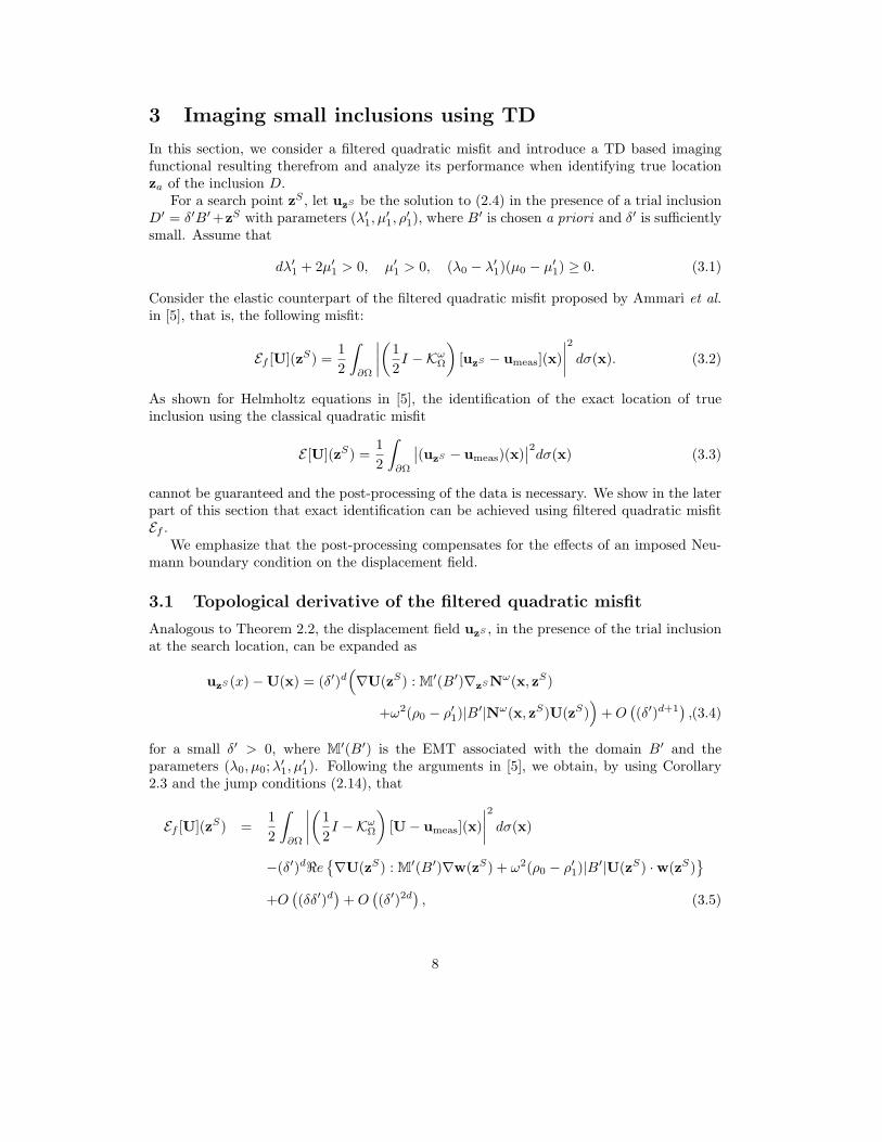
for large n; see, for instance, [5]. The following proposition holds.
Proposition 3.3. Let Uαj be defined in (3.14), where j = 1, 2, · · · , n, for n sufficiently
large. Then, for all zS ∈ Ω far from ∂Ω,
1
n
n∑
j=1
ITD[UPj ](zS) ' 4µ0Cω
3(π
κP)d−2(
κS
κP)2
[1
cP
∣∣=mΓω
0,P (zS − za)∣∣2
+1
cS=m
Γω
0,P (zS − za)
: =mΓω
0,S(zS − za)],(3.16)
10

and
1
n
n∑
j=1
ITD[USj ](zS) ' 4µ0Cω
3(π
κS)d−2
[1
cS
∣∣=mΓω
0,S(zS − za)∣∣2
+1
cP=m
Γω
0,P (zS − za)
: =mΓω
0,S(zS − za)],(3.17)
where C is given by (3.12).
Proof. From (3.15) it follows that
1
n
n∑
j=1
eiκP x·eθj eθj⊗ eθj
' −4(π
κP)d−2=m
1
κ2P
DxGωP (x)
' 4µ0(π
κP)d−2(
κS
κP)2=m
Γω
0,P (x), (3.18)
and
1
n
n∑
j=1
eiκSx·eθj e⊥θj
⊗ e⊥θj
=1
n
n∑
j=1
eiκSx·eθj
(I2 − eθj
⊗ eθj
)
' 4(π
κS)d−2=m
(I2 +
1
κ2S
Dx
)Gω
S(x)
= 4µ0(π
κS)d−2=m
Γω
0,S(x), (3.19)
where the last equality comes from (2.11). Note that, in three dimensions, (3.19) is to beunderstood as follows:
1
n
n∑
j=1
2∑
l=1
eiκSx·eθj e⊥,lθj
⊗ e⊥,lθj
' 4µ0(π
κS)=m
Γω
0,S(x).
Then, using the definition of UPj we compute imaging functional ITD for n plane P−waves
as
1
n
n∑
j=1
ITD[UPj ](zS) = Cω4 1
n
n∑
j=1
<eUPj (zS) ·
[ˆ
∂Ω
Γω0 (x − za)Γω
0 (x − zS)dσ(x)UPj (za)
]
' Cω3 1
n
n∑
j=1
<e eiκP (zS−za)·eθj eθj·[=m
1
cPΓω
0,P (zS − za)
+1
cSΓω
0,S(zS − za)
eθj
]
' Cω3<e[
1
n
n∑
j=1
eiκP (zS−za)·eθj eθj⊗ eθj
]:
[=m
1
cPΓω
0,P (zS − za) +1
cSΓω
0,S(zS − za)
].
11

Here we used the fact that eθj·Aeθj
= eθj⊗eθj
: A for a matrix A, which is easy to check.Finally, exploiting the approximation (3.18), we conclude that
1
n
n∑
j=1
ITD[UPj ](zS) ' 4µ0Cω
3(π
κP)d−2(
κS
κP)2
[1
cP
∣∣=mΓω
0,P (zS − za)∣∣2
+1
cS=m
Γω
0,P (zS − za)
: =mΓω
0,S(zS − za)].
Similarly, we can compute the imaging functional ITD for n plane S−waves exploitingthe approximation (3.19), as
1
n
n∑
j=1
ITD[USj ](zS) = Cω4 1
n
n∑
j=1
<eUSj (zS) ·
[ˆ
∂Ω
Γω0 (x − za)Γω
0 (x − zS)dσ(x)USj (za)
]
' Cω3 1
n
n∑
j=1
<e eiκS(zS−za)·eθj e⊥θj
·[=m
1
cPΓω
0,P (zS − za)
+1
cSΓω
0,S(zS − za)
e⊥θj
]
' Cω3<e[
1
n
n∑
j=1
eiκS(zS−za)·eθj e⊥θ ⊗ e
⊥θ
]:
[=m
1
cPΓω
0,P (zS − za) +1
cSΓω
0,S(zS − za)]
' 4µ0Cω3(π
κS)d−2
[1
cS
∣∣=mΓω
0,S(zS − za)∣∣2
+1
cP=m
Γω
0,P (zS − za)
: =mΓω
0,S(zS − za)].
This completes the proof.
From Proposition 3.3, it is not clear that the imaging functional ITD attains its maximum
at za. Moreover, for both1
n
n∑
j=1
ITD[USj ](zS) and
1
n
n∑
j=1
ITD[UPj ](zS) the resolution at za is
not fine enough due to the presence of the term =mΓω
0,P (zS − za)
: =mΓω
0,S(zS − za).
One way to cancel out this term is to combine1
n
n∑
j=1
ITD[USj ](zS) and
1
n
n∑
j=1
ITD[UPj ](zS)
as follows:
1
n
n∑
j=1
(cS(
κP
π)d−2(
κP
κS)2ITD[UP
j ](zS) − cP (κS
π)d−2ITD[US
j ](zS)
).
12
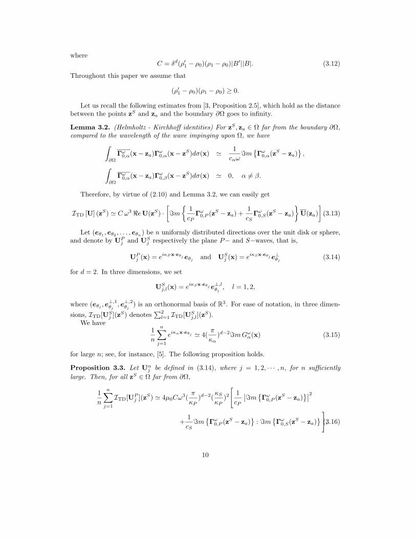
However, one arrives at
1
n
n∑
j=1
(cS(
κP
π)d−2(
κP
κS)2ITD[UP
j ](zS) − cP (κS
π)d−2ITD[US
j ](zS)
)
' 4µ0Cω3
(cScP
∣∣=mΓω
0,P (zS − za)∣∣2 − cP
cS
∣∣=mΓω
0,S(zS − za)∣∣2),
which is not a sum of positive terms and then can not guarantee that the maximum of theobtained imaging functional is at the location of the inclusion.
3.2.2 Case II: Elasticity contrast
Suppose ρ0 = ρ1. Further, we assume for simplicity that M = M′(B′) = M(B). From
Lemma 3.2 we haveˆ
∂Ω
∇zaΓω
0 (x − za)∇zSΓω0 (x − zS)dσ(x) ' 1
cSω=m
∇za
∇zSΓω0,S(zS − za)
+1
cPω=m
∇za
∇zSΓω0,P (zS − za)
.
(3.20)Then, using (3.7) and (3.20), ITD [U] (zS) at zS ∈ Ω becomes
ITD [U] (zS) = δd <e∇U(zS) : M∇w(zS)
= −δd <e∇U(zS) : M
[ˆ
∂Ω
∇zaΓω
0 (x − za)∇zSΓω0 (x − zS)dσ(x) : M∇U(za)
]
' −δd
ω<e∇U(zS) : M
[∇2(=m
Γω
0 (zS − za))
: M∇U(za)
], (3.21)
where
Γω0 (zS − za) =
1
cPΓω
0,P (zS − za) +1
cSΓω
0,S(zS − za). (3.22)
Let us define
Jα,β(zS) :=(M=m
[(∇2Γω
0,α
)(zS − za)
] ):(M=m
[(∇2Γω
0,β
)(zS − za)
] )T
, (3.23)
where AT = (Aklij) if A is the 4-tensor given by A = (Aijkl). Here A : B =
∑ijklAijklBijkl
for any 4-tensors A = (Aijkl) and B = (Bijkl).The following result holds.
Proposition 3.4. Let Uαj be defined in (3.14), where j = 1, 2, · · · , n, for n sufficiently
large. Let Jα,β be defined by (3.23). Then, for all zS ∈ Ω far from ∂Ω,
1
n
n∑
j=1
ITD[UPj ](zS) ' 4δdµ0
ω(π
κP)d−2(
κS
κP)2( 1
cPJP,P (zS) +
1
cSJS,P (zS)
)(3.24)
and1
n
n∑
j=1
ITD[USj ](zS) ' 4δdµ0
ω(π
κS)d−2
( 1
cSJS,S(zS) +
1
cPJS,P (zS)
). (3.25)
13
Proof. Let us compute ITD for n plane P−waves, i.e.
1
n
n∑
j=1
ITD[UPj ](zS) = −δ
d
ω
1
n<e
n∑
j=1
∇UPj (zS) : M
[=m
(∇2Γω
0
)(zS − za)
: M∇UP
j (za)]
' −δd ω
c2P
1
n<e
n∑
j=1
eiκP (zS−za)·eθj eθj⊗ eθj
:
M
(=m
∇2Γω
0 (zS − za)
: Meθj⊗ eθj
). (3.26)
Equivalently,
1
n
n∑
j=1
ITD[UPj ](zS) = −δd ω
c2P
1
n<e
n∑
j=1
eiκP (zS−za)·eθj
d∑
i,k,l,m=1
d∑
i′,k′,l′,m′=1
Aθj
ik mlmik
×=m((
∂2li′Γ
ω0
)(zS − za)
)mk′
ml′m′i′k′ A
θj
l′m′ (3.27)
where the matrix Aθj = (Aθj
ik)ik is defined as Aθj := eθj⊗ eθj
. It follows that
1
n
n∑
j=1
ITD[UPj ](zS) = −δd<e
d∑
i,k,l,m=1
d∑
i′,k′,l′,m′=1
mlmik ml′m′i′k′=m[((
∂2li′Γ
ω0
)(zS − za)
)mk′
]
×(ω
c2P
1
n
n∑
j=1
eiκP (zS−za)·eθjAθj
ikAθj
l′m′
). (3.28)
Recall that for n sufficiently large, we have from (3.18)
1
n
n∑
j=1
eiκP x·eθj eθj⊗ eθj
' 4µ0(π
κP)d−2(
κS
κP)2=m
Γω
0,P (x).
Taking the Hessian of the previous approximation leads to
1
n
n∑
j=1
eiκP x·eθj eθj⊗ eθj
⊗ eθj⊗ eθj
' −4µ0c2Pω2
(π
κP)d−2(
κS
κP)2 =m
∇2Γω
0,P (x)
' −4µ0c4Pω2c2S
(π
κP)d−2 =m
∇2Γω
0,P (x). (3.29)
Then, by virtue of (3.18) and (3.29), we obtain
1
n
n∑
j=1
ITD[UPj ](zS) ' δd 4µ0
ω(π
κP)d−2(
κS
κP)2
d∑
i,k,l,m=1
d∑
i′,k′,l′,m′=1
mlmik ml′m′i′k′
×=m((
∂2li′Γ
ω0
)(zS − za)
)mk′
=m
((∂2
l′iΓω0,P
)(zS − za)
)m′k
' δd 4µ0
ω(π
κP)d−2(
κS
κP)2
d∑
i,k,i′,k′=1
(d∑
l,m=1
mlmik=m((
∂2li′Γ
ω0
)(zS − za)
)mk′
)
×(
d∑
l′,m′=1
ml′m′i′k′=m((
∂2l′iΓ
ω0,P
)(zS − za)
)m′k
).
14

Therefore, by the definition (3.23) of Jα,β , we conclude that
1
n
n∑
j=1
ITD[UPj ](zS) ' δd 4µ0
ω(π
κP)d−2(
κS
κP)2(M=m
∇2Γω
0 (zS − za))
:(M=m
∇2Γω
0,P (zS − za))T
' δd 4µ0
ω(π
κP)d−2(
κS
κP)2(
1
cPJP,P (zS) +
1
cSJS,P (zS)
).
Similarly, consider the case of plane S−waves and compute ITD for n directions. We have
1
n
n∑
j=1
ITD[USj ](zS) = −δ
d
ω
1
n<e
n∑
j=1
∇USj (zS) : M
(=m
(∇2Γω
0
)(zS − za)
: M∇US
j (za))
' −δd ω
c2S
1
n<e
n∑
j=1
eiκS(zS−za)·eθj e⊥θj
⊗ eθj: M
(=m
(∇2Γω
0
)(zS − za)
: M e
⊥θj
⊗ eθj
)
' −δd ω
c2S
1
n<e
n∑
j=1
eiκS(zS−za)·eθj
d∑
i,k,l,m=1
d∑
i′,k′,l′,m′=1
Bθj
ik mlmik
×=m((
∂2li′Γ
ω0
)(zS − za)
)mk′
ml′m′i′k′B
θj
l′m′ (3.30)
where the matrix Bθj = (Bθj
ik )ik is defined as Bθj = eθj⊗ e
⊥θj
. It follows that
1
n
n∑
j=1
ITD[USj ](zS) = −δd
d∑
i,k,l,m=1
d∑
i′,k′,l′,m′=1
mlmik ml′m′i′k′=m[∂2
li′
(Γω
0 (zS − za))
mk′
]
ω
c2S
1
n
n∑
j=1
eiκS(zS−za)·eθjBθj
ikBθj
l′m′
. (3.31)
Now, recall from (3.19) that for n sufficiently large, we have
1
n
n∑
j=1
eiκSx·eθj e⊥θj
⊗ e⊥θj
' 4µ0(π
κS)d−2=m
Γω
0,S(x).
Taking the Hessian of this approximation leads to
1
n
n∑
j=1
eiκSx·eθj eθj⊗ e
⊥θj
⊗ eθj⊗ e
⊥θj
' −4µ0c2Sω2
(π
κS)d−2=m
∇2Γω
0,P (x), (3.32)
where we have made use of the convention
(∇2Γω
0,S
)ijkl
= ∂ik
(Γω
0,S
)jl.
15

Then, by using (3.19), (3.32) and the similar arguments as in the case of P−waves, we arriveat
1
n
n∑
j=1
ITD[USj ](zS) ' δd 4µ0
ω(π
κS)d−2
d∑
i,k,l,m=1
d∑
i′,k′,l′,m′=1
mlmik ml′m′i′k′
×=m((
∂2li′Γ
ω0
))mk′
(zS − za)
×=m((
∂2l′iΓ
ω0,S
))m′k
(zS − za)
' δd 4µ0
ω(π
κS)d−2
(M=m
(∇2Γω
0
)(zS − za)
):
(M=m
(∇2Γω
0,S
)(zS − za)
)T
' δd 4µ0
ω(π
κS)d−2
( 1
cPJP,S(zS) +
1
cSJS,S(zS)
).
This completes the proof.
As observed in Section 3.2.1, Proposition 3.4 shows that the resolution of ITD deterioratesdue to the presence of the coupling term
JP,S(zS) =(M=m
(∇2Γω
0,S
)(zS − za)
):(M=m
(∇2Γω
0,P
)(zS − za)
)T
. (3.33)
3.2.3 Summary
To conclude, we summarize the results of this section below.
- Propositions 3.3 and 3.4 indicate that the imaging function ITD may not attain itsmaximum at the true location, za, of the inclusion D.
- In both cases, the resolution of the localization of elastic anomaly D degenerates dueto the presence of the coupling terms =m
Γω
0,P (zS − za)
: =mΓω
0,S(zS − za)
and
JP,S(zS), respectively.
- In order to enhance imaging resolution to its optimum and insure that the imagingfunctional attains its maximum only at the location of the inclusion, one must eradicatethe coupling terms.
4 Modified imaging framework
In this section, in order to achieve a better localization and resolution properties, we intro-duce a modified imaging framework based on a weighted Helmholtz decomposition of theTD imaging functional. We will show that the modified framework leads to both a betterlocalization (in the sense that the modified imaging functional attains its maximum at thelocation of the inclusion) and a better resolution than the classical TD based sensitivityframework. It is worthwhile mentioning that the classical framework performs quite well
16

for the case of Helmholtz equation [5] and the resolution and localization deteriorationsare purely dependent on the elastic nature of the problem, that is, due to the coupling ofpressure and shear waves propagating with different wave speeds and polarization directions.
It should be noted that in the case of a density contrast only, the modified imaging func-tional is still a topological derivative based one, i.e., obtained as the topological derivativeof a discrepancy functional. This holds because of the nonconversion of waves (from shear tocompressional and vice versa) in the presence of only a small inclusion with a contrast den-sity. However, in the presence of a small inclusion with different Lame coefficients with thebackground medium, there is a mode conversion; see, for instance, [21]. As a consequence,the modified functional proposed here can not be written in such a case as the topologicalderivative of a discrepancy functional. It is rather a Kirchhoff-type imaging functional.
4.1 Weighted imaging functional
Following [3], we introduce a weighted topological derivative imaging functional IW, andjustify that it provides a better localization of the obstacle D than ITD. This new functionalIW can be seen as a correction based on a weighted Helmholtz decomposition of ITD. Infact, using the standard L2-theory of the Helmholtz decomposition (see, for instance, [16]),we find that in the search domain the pressure and the shear components of w, defined by(3.6), can be written as
w = ∇× ψw + ∇φw. (4.1)
We define respectively the Helmholtz decomposition operators HP and HS by
HP [w] := ∇φw and HS [w] := ∇× ψw. (4.2)
Actually, the decomposition w = HP [w] + HS [w] can be found by solving a Neumannproblem in the search domain [16]. Then we multiply the components of w with cP and cS ,the background pressure and the shear wave speeds respectively. Finally, we define IW by
IW [U] = cP<e∇HP [U] : M
′(B′)∇HP [w] + ω2
(ρ′1ρ0
− 1
)|B′|HP [U] · HP [w]
+ cS<e∇HS [U] : M
′(B′)∇HS [w] + ω2
(ρ′1ρ0
− 1
)|B′|HS [U] · HS [w]
.(4.3)
We rigorously explain in the next section why this new functional should be better thanimaging functional ITD.
4.2 Sensitivity analysis of weighted imaging functional
In this section, we explain why imaging functional IW attains its maximum at the locationza of the true inclusion with a better resolution than ITD. In fact, as shown in the later partof this section, IW behaves like the square of the imaginary part of a pressure or a shearGreen function depending upon the incident wave. Consequently, it provides a resolution ofthe order of half a wavelength. For simplicity, we once again consider special cases of onlydensity contrast and only elasticity contrast.
17

4.2.1 Case I: Density contrast
Suppose λ0 = λ1 and µ0 = µ1. Recall that in this case, the wave function w is given by(3.10). Note that Hα[Γω
0 ] = Γω0,α, α ∈ P, S. Therefore, the imaging functional IW at
zS ∈ Ω turns out to be
IW [U] (zS) = C ω4<e(cPHP [U](zS) ·
[(ˆ
∂Ω
Γω0 (x − za)Γω
0,P (x − zS)dσ(x))U(za)
]
+cSHS [U](zS) ·[( ˆ
∂Ω
Γω0 (x − za)Γω
0,S(x − zS)dσ(x))U(za)
]). (4.4)
By using Lemma 3.2, we can easily get
IW [U] (zS) ' C ω3<e(HP [U](zS) ·
[=m
Γω
0,P (zS − za)U(za)
]
+HS [U](zS) ·[=m
Γω
0,S(zS − za)U(za)
]). (4.5)
Consider n uniformly distributed directions (eθ1,eθ2
, . . . ,eθn) on the unit disk or sphere
for n sufficiently large. Then, the following proposition holds.
Proposition 4.1. Let Uαj be defined in (3.14), where j = 1, 2, · · · , n, for n sufficiently
large. Then, for all zS ∈ Ω far from ∂Ω,
1
n
n∑
j=1
IW[UPj ](zS) ' 4µ0Cω
3(π
κP)d−2(
κS
κP)2∣∣=m
Γω
0,P (zS − za)∣∣2 , (4.6)
and1
n
n∑
j=1
IW[USj ](zS) ' 4µ0Cω
3(π
κS)d−2
∣∣=mΓω
0,S(zS − za)∣∣2 , (4.7)
where C is given by (3.12).
Proof. By using similar arguments as in Proposition 3.3 and (4.5), we show that the weightedimaging functional IW for n plane P−waves is given by
1
n
n∑
j=1
IW[UPj ](zS) = C ω3 1
n<e
n∑
j=1
UPj (zS) ·
[=m
Γω
0,P (zS − za)UP
j (za)]
' Cω3 1
n<e
n∑
j=1
eiκP (zS−za).eθj eθj·[=m
Γω
0,P (zS − za)
eθj
]
' 4µ0Cω3(π
κP)d−2(
κS
κP)2∣∣=m
Γω
0,P (zS − za)∣∣2 ,
18

and for n plane S−waves
1
n
n∑
j=1
IW[USj ](zS) = Cω3 1
n
n∑
j=1
USj (zS) ·
[=m
Γω
0,S(zS − za)USs
j (za)]
' Cω3 1
n
n∑
j=1
eiκP (zS−za)·eθj e⊥θj
·[=m
Γω
0,S(zS − za)
e⊥θj
]
' 4µ0Cω3(π
κS)d−2
∣∣=mΓω
0,S(zS − za)∣∣2 .
Proposition 4.1 shows that IW, attains its maximum at za (see Figure 1) and the cou-pling term =m
Γω
0,P (zS − za)
: =mΓω
0,S(zS − za), responsible for the decreased reso-
lution in ITD, is absent. Moreover, the resolution using weighted imaging functional IW
is the Rayleigh one, that is, restricted by the diffraction limit of half a wavelength of the
wave impinging upon Ω, thanks to the term∣∣=m
Γω
0,α(zS − za)∣∣2. Finally, it is worth
mentioning that IW is a topological derivative based imaging functional. In fact, it is thetopological derivative of the discrepancy functional cSEf [US ] + cPEf [UP ], where US is anS-plane wave and UP is a P -plane wave.
−10 −5 0 5 10
−10
−8
−6
−4
−2
0
2
4
6
8
10−10 −5 0 5 10
−10
−8
−6
−4
−2
0
2
4
6
8
10
Figure 1: Typical plots of∣∣=m
Γω
0,S(zS − za)∣∣2 (on the left) and
∣∣=mΓω
0,P (zS − za)∣∣2
(on the right) for za = 0.
19

4.2.2 Case II: Elasticity contrast
Suppose ρ0 = ρ1 and assume for simplicity that M = M′(B′) = M(B). Then, the weighted
imaging functional IW reduces to
IW(zS) = −δd
[cP∇HP [U(zS)] : M∇HP [w(zS)] + cS∇HS [U(zS)] : M∇HSw(zS)]
]
= −δd
[cP∇HP [U(zS)] : M
(ˆ
∂Ω
∇zaΓω
0 (x − za)∇zSΓω0,P (x − zS)dσ(x) : M∇U(za)
)
+cS∇HS [U(zS)] : M
(ˆ
∂Ω
∇zaΓω
0 (x − za)∇zSΓω0,S(x − zS)dσ(x) : M∇U(za)
)]
= −δd
[∇HP [U(zS)] : M
(=m
(∇2Γω
0,P
)(zS − za)
: M∇U(za)
)
+∇HS [U(zS)] : M
(=m
(∇2Γω
0,S
)(zS − za)
: M∇U(za)
)]. (4.8)
We observed in Section 3.2.2 that the resolution of ITD is compromised because ofthe coupling term JS,P (zS). We can cancel out this term by using the weighted imagingfunctional IW. For example, using analogous arguments as in Proposition 3.4, we can easilyprove the following result.
Proposition 4.2. Let Uαj be defined in (3.14), where j = 1, 2, · · · , n, for n sufficiently
large. Let Jα,β be defined by (3.23). Then, for all zS ∈ Ω far from ∂Ω,
1
n
n∑
j=1
IW[Uαj ](zS) ' 4δdµ0
ω(π
κα)d−2(
κS
κα)2Jα,α(zS), α ∈ P, S. (4.9)
It can be established that IW attains its maximum at zS = za. Consider, for example,the canonical case of a circular or spherical inclusion. The following propositions hold.
Proposition 4.3. Let D be a disk or a sphere. Then for all search points zS ∈ Ω,
JP,P (zS) = a2∣∣∣∇2
(=mΓω
0,P
)(zS − za)
∣∣∣2
+ 2ab∣∣∣∆(=mΓω
0,P
)(zS − za)
∣∣∣2
+b2∣∣∣∆Tr
(=mΓω
0,P
)(zS − za)
∣∣∣2
, (4.10)
where Tr represents the trace operator and the constants a and b are defined in (2.19).
Proof. Since
(∇2Γω
0,P
)ijkl
= ∂ik
(Γω
0,P
)jl, (4.11)
20

it follows from (2.19) that
(M∇2Γω
0,P
)ijkl
=∑
p,q
mijpq
(∇2Γω
0,P
)pqkl
(4.12)
=a
2
(∂ik
(Γω
0,P
)jl
+ ∂jk
(Γω
0,P
)il
)+ b
d∑
q=1
∂qk
(Γω
0,P
)qlδij
=a
2∂k
((∇Γω
0,P el
)ij
+(∇Γω
0,P el
)Tij
)+ b∂k∇ ·
((Γω
0,P el
))δij ,(4.13)
where el is the unit vector in the direction xl.Now, since Γω
0,pel is a P−wave, its rotational part vanishes and the gradient is symmetric,i.e.,
∇× (Γω0,P el) = 0 and
(∇Γω
0,P el
)ij
=(∇Γω
0,P el
)ji
=(∇Γω
0,P el
)Tij. (4.14)
Consequently,
∇∇ ·( (
Γω0,P el
) )= ∇×
(∇×
(Γω
0,P el
) )+ ∆
(Γω
0,P el
)= ∆
(Γω
0,P el
), (4.15)
which, together with (4.13) and (4.14), implies
M∇2Γω0,P = a∇2Γω
0,P + b I2 ⊗ ∆Γω0,P . (4.16)
Moreover, by the definition of Γω0,P , its Hessian, ∇2Γω
0,P , is also symmetric. Indeed,
(∇2Γω
0,P
)T
ijkl= ∂ki
(Γω
0,P
)lj
= −µ0
κ2S
∂kijlGωP =
(∇2Γω
0,P
)ijkl
. (4.17)
Therefore, by virtue of (4.16) and (4.17), JP,P can be rewritten as
JP,P (zS) =(a=m
(∇2Γω
0,P
)(zS − za) + bI2 ⊗=m
(∆Γω
0,P
)(zS − za)
)
:(a=m
(∇2Γω
0,P
)(zS − za) + b=m
(∆Γω
0,P
)(zS − za) ⊗ I2
). (4.18)
Finally, we observe that
(∇2=m
Γω
0,P
):(∇2=m
Γω
0,P
)T
=∣∣∣∇2=m
Γω
0,P
∣∣∣2
, (4.19)
21

∇2=mΓω0,P :
(I2 ⊗ ∆=mΓω
0,P )
= ∇2=mΓω0,P :
(∆=mΓω
0,P ⊗ I2
)
=
d∑
i,j,k,l=1
(=m
(∂ikΓ
ω0,P
)jl
)δij∆=m
(Γω
0,P
)kl
=
d∑
k,l=1
(d∑
i=1
(=m
(∂ikΓ
ω0,P
)il
))
∆=m(Γω
0,P
)kl
=
d∑
k,l=1
(∆=m
(Γω
0,P
)kl
)2
=∣∣∣∆=m Γω
0,P ∣∣∣2
, (4.20)
and
(I2 ⊗ ∆=mΓω
0,P )
:(∆=mΓω
0,P ⊗ I2
)=
d∑
i,j,k,l=1
δij∆=m(Γω
0,P
)klδkl∆=m
(Γω
0,P
)ij
=
d∑
i,k=1
∆=m(Γω
0,P
)kk
∆=m(Γω
0,P
)ii
=∣∣∣∆Tr(=m Γω
0,P )∣∣∣2
. (4.21)
We arrive at the conclusion by substituting (4.19), (4.20) and (4.21) in (4.18).
Proposition 4.4. Let D be a disk or a sphere. Then, for all search points zS ∈ Ω,
JS,S(zS) =a2
µ20
[1
κ4S
∣∣∣∇4=mGω
S(zS − za) ∣∣∣
2
+(d− 6)
4
∣∣∣∇2=mGω
S(zS − za) ∣∣∣
2
+κ4
S
4
∣∣∣=mGω
S(zS − za) ∣∣∣
2]
=a2
µ20
[1
κ4S
∑
ijkl,k 6=l
∣∣∣∂ijkl=mGω
S(zS − za) ∣∣∣
2
+(d− 2)
4
∣∣∣∇2=mGω
S(zS − za) ∣∣∣
2
+κ4
S
4
∣∣∣=mGω
S(zS − za) ∣∣∣
2], (4.22)
where a is the constant as in (2.19).
Proof. As before, we have(
M∇2Γω0,S
)
ijkl
=a
2
(∂ik
(Γω
0,S
)jl
+ ∂jk
(Γω
0,S
)il
)+ b ∂k∇ ·
((Γω
0,Sel
))δij
=a
2
(∂ik
(Γω
0,S
)jl
+ ∂jk
(Γω
0,S
)il
). (4.23)
22
and
(M∇2Γω
0,S
)T
ijkl=a
2
(∂ik
(Γω
0,S
)jl
+ ∂il
(Γω
0,S
)jk
). (4.24)
Here we have used the facts that Γω0,Sel is a S−wave and, Γω
0,S and its Hessian are symmetric,i.e.,
∂ik
(Γω
0,S
)jl
= ∂ki
(Γω
0,S
)jl
= ∂ik
(Γω
0,S
)lj
= ∂ki
(Γω
0,S
)lj. (4.25)
Substituting, (4.23) and (4.24) in (3.23), we obtain
JS,S(zS) =a2
4
d∑
i,j,k,l=1
=m((
∂ikΓω0,S
)(zS − za)
)jl
+((∂jkΓ
ω0,S
)(zS − za)
)il
×=m((
∂ikΓω0,S
)(zS − za)
)jl
+((∂ilΓ
ω0,S
)(zS − za)
)jk
:=a2
4
(T1(z
S) + 2T2(zS) + T3(z
S)), (4.26)
where
T1(zS) =
d∑
i,j,k,l=1
(=m
(∂ikΓ
ω0,S
)jl
(zS − za))(
=m(∂ikΓ
ω0,S
)jl
(zS − za))
,
T2(zS) =
d∑
i,j,k,l=1
(=m
(∂ikΓ
ω0,S
)jl
(zS − za))(
=m(∂ilΓ
ω0,S
)jk
(zS − za))
,
T3(zS) =
d∑
i,j,k,l=1
(=m
(∂jkΓ
ω0,S
)il(zS − za)
)(=m
(∂ilΓ
ω0,S
)jk
(zS − za))
.
Notice that
=mΓω
0,S(x)
=1
µ0κ2S
(κ2SI2 + Dx)=m Gω
S(x) ,
and =m GωS satisfies
∆=m GωS (zS − za) + κ2
S=m GωS (zS − za) = 0 for zS 6= za. (4.27)
Therefore, the first term T1 can be computed as follows
T1(zS) =
∣∣∣∇2(=mΓω
0,S
)(zS − za)
∣∣∣2
=1
µ20κ
4S
d∑
i,j,k,l=1
[(∂ijkl
(=mGω
S
)(zS − za)
)2
+ κ4Sδjl
(∂ik
(=mGω
S
)(zS − za)
)2
+2κ2Sδjl∂ik
(=mGω
S
)(zS − za)∂ijkl
(=mGω
S
)(zS − za)
].
23

We also have
d∑
i,j,k,l=1
2δjl∂ik
(=mGω
S
)(zS − za)
(∂ijkl=m
(Gω
S
)(zS − za)
)
= 2d∑
i,k=1
(∂ik
(=mGω
S
)(zS − za)
)(∂ik
d∑
l=1
∂ll
(=mGω
S
)(zS − za)
)
= −2κ2S
d∑
i,k=1
(∂ik
(=mGω
S
)(zS − za)
)2
,
and
d∑
i,j,k,l=1
δjl
(∂ik
(=mGω
S
)(zS − za)
)2
= d
d∑
i,k=1
(∂ik
(=mGω
S
)(zS − za)
)2
.
Consequently, we have
T1(zS) =
∣∣∣∇2(=mΓω
0,S
)(zS − za)
∣∣∣2
= 1µ2
0κ4
S
∣∣∣∇4(=mGω
S
)(zS − za)
∣∣∣2
+ (d−2)µ2
0
∑di,k=1
(∂ik
(=mGω
S
)(zS − za)
)2
.
(4.28)
Estimation of the term T2 is quite similar. Indeed,
T2(zS) =
1
µ20κ
4S
d∑
i,j,k,l=1
[(∂ijkl
(=mGω
S
)(zS − za)
)2
+2κ2Sδjl∂ik
(=mGω
S
)(zS − za)∂ijkl
(=mGω
S
)(zS − za)
+κ4Sδjlδjk
(∂ik
(=mGω
S
)(zS − za)
)(∂il
(=mGω
S
)(zS − za)
)].
Finally, using
d∑
i,j,k,l=1
δjlδjk
(∂ik
(=mGω
S
)(zS − za)
)(∂il
(=mGω
S
)(zS − za)
)=
d∑
i,k=1
(∂ik
(=mGω
S
)(zS − za)
)2
,
we obtain that
T2(zS) =
1
µ20κ
4S
∣∣∣∇4(=mGω
S
)(zS − za)
∣∣∣2
− 1
µ20
∣∣∣∇2(=mGω
S
)(zS − za)
∣∣∣2
. (4.29)
24
Similarly,
T3(zS) =
1
µ20κ
4S
d∑
i,j,k,l=1
[(∂ijkl
(=mGω
S
)(zS − za)
)2
+2κ2Sδjl∂ik
(=mGω
S
)(zS − za)
(∂ijkl
(=mGω
S
)(zS − za)
)
+κ4Sδilδjk
(∂jk
(=mGω
S
)(zS − za)
)(∂il
(=mGω
S
)(zS − za)
)].
By virtue of
d∑
i,j,k,l=1
δilδjk
(∂jk
(=mGω
S
)(zS − za)
) (∂il
(=mGω
S
)(zS − za)
)
=d∑
i,k=1
(∂kk
(=mGω
S
)(zS − za)
)(∂ii
(=mGω
S
)(zS − za)
)
= κ4S
(=mGω
S(zS − za))2
,
we have
T3(zS) =
1
µ20κ
4S
∣∣∣∇4(=mGω
S
)(zS − za)
∣∣∣2
− 2
µ20
∣∣∣∇2(=mGω
S
)(zS − za)
∣∣∣2
+κ4
S
µ20
∣∣∣=mGωS(zS − za)
∣∣∣2
. (4.30)
We conclude the proof by substituting (4.28), (4.29) and (4.30) in (4.26) and using again(4.27).
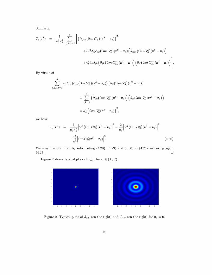
Figure 2 shows typical plots of Jα,α for α ∈ P, S.
−8 −6 −4 −2 0 2 4 6 8
−8
−6
−4
−2
0
2
4
6
8
−8 −6 −4 −2 0 2 4 6 8
−8
−6
−4
−2
0
2
4
6
8
Figure 2: Typical plots of JSS (on the right) and JPP (on the right) for za = 0.
25

5 Statistical stability with measurement noise
Let UPj and US
j be as before. Let Uj be plane waves. Define
IWF[Uj](zS) =1
n
n∑
j=1
IW[Uj ](zS). (5.1)
In the previous section, we have analyzed the resolution of the imaging functional IWF inthe ideal situation where the measurement umeas is accurate. Here, we analyze how theresult will be modified when the measurement is corrupted by noise.
5.1 Measurement noise model
We consider the simplest model for the measurement noise. Let utrue be the accurate valueof the elastic displacement field. The measurement umeas is then
umeas(x) = utrue(x) + νnoise(x), (5.2)
that is the accurate value corrupted by measurement noise modeled as νnoise(x), x ∈ ∂Ω.Note that νnoise(x) is valued in C
d, d = 2, 3.Let E denote the expectation with respect to the statistics of the measurement noise.
We assume that νnoise(x),x ∈ ∂Ω is mean zero circular Gaussian and satisfies
E[νnoise(y) ⊗ νnoise(y′)] = σ2noiseδy(y′)I2. (5.3)
This means that firstly the measurement noises at different locations on the boundary areuncorrelated; secondly, different components of the measurement noise are uncorrelated, andthirdly the real and imaginary parts are uncorrelated. Finally, the noise has variance σ2
noise.In the imaging functional IWF, the elastic medium is probed by multiple plane waves with
different propagating directions, and consequently multiple measurements are obtained atthe boundary accordingly. We assume that two measurements corresponding to two differentplane wave propagations are uncorrelated. Therefore, it holds that
E[νjnoise(y) ⊗ ν
lnoise(y
′)] = σ2noiseδjlδy(y′)I2, (5.4)
where j and l are labels for the measurements and δjl is the Kronecker symbol.
5.2 Propagation of measurement noise in the back-propagation step
The measurement noise affects the topological derivative based imaging functional throughthe back-propagation step which builds the function w in (3.6). Due to the noise, we have
w(x) = SωΩ
[(1
2I −Kω
Ω
)[U − utrue − νnoise]
](x) = wtrue(x) + wnoise(x), (5.5)
for x ∈ Ω. Here, wtrue is the result of back-propagating only the accurate data while wnoise
is that of back-propagating the measurement noise. In particular,
wnoise(x) = −SωΩ
[(1
2I −Kω
Ω
)[νnoise]
](x), x ∈ Ω. (5.6)
26

To analyze the statistics of wnoise, we proceed in two steps. First define
νnoise,1(x) =
(1
2I −Kω
Ω
)[νnoise](x), x ∈ ∂Ω. (5.7)
Then, due to linearity, νnoise,1 is also a mean-zero circular Gaussian random process. Itscovariance function can be calculated as
E[νnoise,1(y) ⊗ νnoise,1(y′)] =1
4E[νnoise(y) ⊗ νnoise(y′)] − 1
2E[Kω
Ω[νnoise](y) ⊗ νnoise(y′)]
−1
2E[νnoise(y) ⊗Kω
Ω[νnoise](y′)] + E[KωΩ[νnoise](y) ⊗Kω
Ω[νnoise](y′)].
The terms on the right-hand side can be evaluated using the statistics of νnoise and theexplicit expression of Kω
Ω. Let us calculate the last term. It has the expression
E
[ˆ
∂Ω
ˆ
∂Ω
[∂Γω
0
∂νx(y − x)νnoise(x)
]⊗[∂Γω
0
∂νx′
(y′ − x′)νnoise(x′)
]dσ(x)dσ(x′)
].
Using the coordinate representations and the summation convention, we can calculate thejkth element of this matrix by
ˆ
∂Ω
ˆ
∂Ω
[∂Γω
0
∂νx(y − x)
]
jl
[∂Γω
0
∂νx′
(y′ − x′)
]
ks
E[νnoise(x) ⊗ νnoise(x′)]lsdσ(x)dσ(x′)
=σ2noise
ˆ
∂Ω
[∂Γω
0
∂νx(y − x)
]
js
[∂Γω
0
∂νx(y′ − x)
]
ks
dσ(x)
=σ2noise
ˆ
∂Ω
∂Γω0
∂νx(y − x)
∂Γω0
∂νx(x − y′)dσ(x).
In the last step, we used the reciprocity relation
Γω0 (y − x) = [Γω
0 (x − y)]T , (5.8)
for any x,y ∈ Rd.
The other terms in the covariance function of νnoise,1 can be similarly calculated. Con-sequently, we have
E[νnoise,1(y) ⊗ νnoise,1(y′)] =σ2
noise
4δy(y′)I2 −
σ2noise
2
[∂Γω
0
∂νy′
(y − y′) +∂Γω
0
∂νy(y − y′)
]
+ σ2noise
ˆ
∂Ω
∂Γω0
∂νx(y − x)
∂Γω0
∂νx(x − y′)dσ(x).
(5.9)
From the expression of IWF and IW, we see that only the Helmholtz decompositionof wmeas, that is HP [w] and HS [w], are used in the imaging functional. Define wα =Hα[w], α ∈ P, S. Using the decomposition in (5.5), we can similarly define wα
true andwα
noise. In particular, we find that
wαnoise(x) = −
ˆ
∂Ω
Γω0,α(x − y)νnoise,1(y)dσ(y), x ∈ Ω.
27

This is a mean zero Cd-valued circular Gaussian random field with parameters in Ω. The
jkth element of its covariance function is evaluated by
E[wαnoise(x)⊗wα
noise(x′)]jk =
ˆ
(∂Ω)2(Γω
0,α(x−y))jl(Γω0,α(x′−y′))ksE[νnoise,1(y)⊗νnoise,1(y
′)]ls.
Using the statistics of νnoise,1 derived above, we find that
E[wαnoise(x) ⊗ wα
noise(x′)] =
σ2noise
4
ˆ
∂Ω
Γω0,α(x − y)Γω
0,α(y − x′)dσ(y)
−σ2noise
2
ˆ
(∂Ω)2Γω
0,α(x − y)[∂Γω
0
∂νy(y − y′) +
∂Γω0
∂νy′
(y − y′)]Γω
0,α(y′ − x′)dσ(y)dσ(y′)
+σ2noise
ˆ
(∂Ω)3Γω
0,α(x − y)∂Γω
0
∂νz(y − z)
∂Γω0
∂νz(z − y′)Γω
0,α(y′ − x′)dσ(z)dσ(y)dσ(y′).
Thanks to the Helmholtz-Kirchhoff identities, the above expression is simplified to
E[wαnoise(x) ⊗ wα
noise(x′)] =
σ2noise
4cαω=mΓω
0,α(x − x′)
−σ2noise
2cαω
ˆ
∂Ω
Γω0,α(x − y)
∂=mΓω0,α(y − x′)∂νy
dσ(y)
−σ2noise
2cαω
ˆ
∂Ω
∂=mΓω0,α(x − y′)∂νy′
Γω0,α(y′ − x′)dσ(y′)
+σ2
noise
(cαω)2
ˆ
∂Ω
∂=mΓω0,α(x − z)∂νz
∂=mΓω0,α(z − x′)∂νz
dσ(z).
Assuming that x,x′ are far away from the boundary, we have from [3] the asymptotic formulathat
∂Γω0,α(x − y)
∂νy' icαωΓω
0,α(x − y), (5.10)
where the error is of order o(|x−y|1/2−d). Using this asymptotic formula and the Helmholtz-Kirchhoff identity (taking the imaginary part of the identity), we obtain that
E[wαnoise(x) ⊗ wα
noise(x′)] =
σ2noise
4cαω=mΓω
0,α(x − x′). (5.11)
5.3 Stability analysis
Now we are ready to analyze the statistical stability of the imaging functional IWF. Asbefore, we consider separate cases where the medium has only density contrast or onlyelastic contrast.
5.3.1 Case I: Density contrast
Using the facts that the plane waves UP ’s are irrotational and that the plane waves US ’sare solenoidal, we see that for a searching point z ∈ Ω, and α ∈ P, S,
IWF[Uαj ](z) = cαω
2
(ρ′1ρ0
− 1
)|B′| 1
n
n∑
j=1
<eUαj (z) · (wα
j,true(z) + wαj,noise(z)).
28

We observe the following: The contribution of wαj,true are exactly those in Proposition 4.1.
On the other hand, the contribution of wαj,noise forms a field corrupting the true image.
With Cα := cαω2|B′|(ρ′1/ρ0 − 1), the covariance function of the corrupted image, can be
calculated as follows. Let z′ ∈ Ω. We have
Cov(IWF[Uαj ](z), IWF[Uα
j ](z′)) = C2α
1
n2
n∑
j,l=1
E[<eUαj · wα
j,noise<eUαl · wα
l,noise]
=C2α
1
2n2
n∑
j=1
<eUα
j (z) · E[wαj,noise(z) ⊗ wα
j,noise(z′)]Uα
j (z′).
To get the second equality, we used the fact that wαj,noise and wα
l,noise are uncorrelated unlessj = l. Thanks to the statistics (5.11), the covariance of the image is given by
C2α
σ2noise
4cαω
1
2n2<e
n∑
j=1
eiκα(z−z′)·eθj e
αθj
· [=mΓω0,α(z − z′)eα
θj],
where ePθj
= eθjand e
Sθj
= e⊥θj
.Using the same arguments as those in the proof of Proposition 4.1, we obtain that
Cov(IWF[Uαj ](z), IWF[Uα
j ](z′)) = C ′α
σ2noise
2n|=mΓω
0,α(z − z′)|2, (5.12)
where the constant
C ′α = cαω
3µ0|B′|2(ρ′1
ρ0− 1)2(
π
κα)d−2(
κS
κα)2.
The following remarks are in order. Firstly, the perturbation due to noise has smalltypical values of order σnoise/
√2n and slightly affects the peak of the imaging functional
IWF. Secondly, the typical shape of the hot spot in the perturbation due to the noise isexactly of the form of the main peak of IWF obtained in the absence of noise. Thirdly, theuse of multiple directional plane waves reduced the effect of measurement noise on the imagequality.
From (5.12) it follows that the variance of the imaging functional IWF at the searchpoint z is given by
Var(IWF[Uαj ](z)) = C ′
α
σ2noise
2n|=mΓω
0,α(0)|2. (5.13)
Define the Signal-to-Noise Ratio (SNR) by
SNR :=E[IWF[Uα
j ](za)]
Var(IWF[Uαj ](za))1/2
,
where za is the true location of the inclusion. From (4.6), (4.7), and (5.13), we have
SNR =4√
2πd−2nω5−dρ30c
d−1α δd|B||ρ1 − ρ0|
σnoise|=mΓω
0,α(0)|. (5.14)
From (5.14), the SNR is proportional to the contrast |ρ1−ρ0| and the volume of the inclusionδd|B|, over the standard deviation of the noise, σnoise.
29
5.3.2 Case II: Elasticity contrast
In the case of elastic contrast, the imaging functional becomes for z ∈ Ω
IWF[Uαj ](z) = cα
1
n
n∑
j=1
∇Uαj (z) : M
′(B′)(∇wαj,true(z) + ∇wα
j,noise(z)).
Here, wαj,true and wα
j,noise are defined in the last section. They correspond to the backpropa-gation of pure data and that of the measurement noise. The contribution of wα
j,true is exactlythe imaging functional with unperturbed data and it is investigated in Proposition 4.2. Thecontribution of wα
j,noise perturbs the true image. For z, z′ ∈ Ω, the covariance function ofthe TD noisy image is given by
Cov(IWF[Uαj ](z), IWF[Uα
j ](z′))
=c2α1
n2
n∑
j,l=1
E[<e∇Uαj (z) : M
′∇wαj,noise(z)<e∇Uα
l (z′) : M′∇wα
l,noise(z′)]
=c2α1
2n2
n∑
j,l=1
<eE[(∇Uαj (z) : M
′∇wαj,noise(z))(∇Uα
l (z′) : M′∇wαl,noise(z
′))]
=c2α1
2n2
n∑
j=1
<e∇Uα
j (z) : M′[E[∇wα
j,noise(z)∇wαj,noise(z
′)] : M′∇Uα
j (z′)]
.
Using (5.11), we find that
E[∇wαj,noise(z)∇wα
j,noise(z′)] =
σ2noise
4cαω=m∇z∇z′Γω
0,α(z − z′).
After substituting this term into the expression of the covariance function, we find that itbecomes
−cασ2noise
4ω
1
2n
n∑
j=1
<e∇Uα
j (z) : M′[=m
∇2Γω
0,α(z − z′)
: M′∇Uα
j (z′)]
.
The sum has exactly the form that was analyzed in the proof of Proposition 3.4. Usingsimilar techniques, we finally obtain that
Cov(IWF[Uαj ](z), IWF[Uα
j ](z′)) = µ0
(cαω
)3( πκα
)d−2(κS
κα)2σ2
noise
2nJα,α(z, z′), (5.15)
where Jα,α is defined by (3.23). The variance of the TD image can also be obtained from(5.15). As in the case of density contrast, the typical shape of hot spots in the imagecorrupted by noise is the same as the main peak of the true image. Further, the effect ofmeasurement noise is reduced by a factor of
√n by using n plane waves. In particular, the
SNR of the TD image is given by
SNR =δd√µ0ω√
c3α
( πκα
) d−2
2κS
κα
4√
2n
σnoise
√Jα,α(za, za). (5.16)
30

6 Statistical stability with medium noise
In the previous section, we demonstrated that the proposed imaging functional using multi-directional plane waves is statistically stable with respect to uncorrelated measurementnoises. Now we investigate the case of medium noise, where the constitutional parametersof the elastic medium fluctuate around a constant background.
6.1 Medium noise model
For simplicity, we consider a medium that fluctuates in the density parameter only. That is,
ρ(x) = ρ0[1 + γ(x)], (6.1)
where ρ0 is the constant background and ρ0γ(x) is the random fluctuation in the density.Note that γ is real valued.
Throughout this section, we will call the homogeneous medium with parameters (λ0, µ0, ρ0)the reference medium. The background medium refers to the one without inclusion but withdensity fluctuation. Consequently, the background Neumann problem of elastic waves is nolonger (2.21). Indeed, that equation corresponds to the reference medium and its solutionwill be denoted by U(0). The new background solution is
(Lλ0,µ0+ ρ0ω
2[1 + γ])U = 0, on Ω,
∂U
∂ν= g on ∂Ω,
(6.2)
Similarly, the Neumann function associated to the problem in the reference medium willbe denoted by Nω,(0). By an abuse of notation, we denote Nω as the Neumann functionassociated to the background medium, that is,
(Lλ0,µ0+ ρ0ω
2[1 + γ(x)])Nω(x,y) = δy(x)I2, x ∈ Ω, x 6= y,
∂Nω
∂ν(x,y) = 0 x ∈ ∂Ω.
(6.3)
We assume that γ has small amplitude so that the Born approximation is valid. Inparticular, we have
Nω(x,y) ' Nω,(0)(x,y) − ρ0ω2
ˆ
Ω
Nω,(0)(x, z)γ(z)Nω,(0)(z,y)dy. (6.4)
As a consequence, we also have that U ' U(0) − U(1) where
U(1)(x) = ρ0ω2
ˆ
Ω
Nω,(0)(x, z)γ(z)U(0)(z)dz. (6.5)
Let σγ denotes the typical size of γ, the remainders in the above approximations are of ordero(σγ).
31

6.2 Statistics of the speckle field in the case of a density contrast
only
We assume that the inclusion has density contrast only. The backpropagation step constructsw as follows:
w(x) =
ˆ
∂Ω
Γω0 (x, z)(
1
2I −Kω,(0)
Ω )[U(0) − umeas](z)dσ(z), x ∈ Ω. (6.6)
We emphasize that the backpropagation step uses the reference fundamental solutions, andthe differential measurement is with respect to the reference solution. These are necessarysteps because of the fluctuation in the background medium or equivalently, because of thefact that the background solution is unknown.
Writing the difference between U(0) and umeas as the sum of U(0) − U and U − umeas.These two differences are estimated by U(1) in (6.5) and by (2.22), respectively. UsingLemma 2.1, we find that
w(x) = ρ0ω2
ˆ
∂Ω
Γω0 (x − z)
ˆ
Ω
Γω0 (z − y)U(0)(y)γ(y)dydσ(z)
+ Cδd
ˆ
∂Ω
Γω0 (x − z)Γω
0 (z − za)U(0)(za)dσ(z) +O(σγδd) + o(σγ), x ∈ Ω,
(6.7)
where C = ω2(ρ0 − ρ1)|B|. The second term is the leading contribution of U− umeas givenby approximating the unknown Neumann function and the background solution by thoseassociated to the reference medium. The leading error in this approximation is of orderO(σγδ
d) and can be written explicitly as
−Cρ0ω2δd
ˆ
∂Ω
Γω0 (x, z)
ˆ
Ω
Γω0 (z,y)Nω,(0)(y, za)U(0)(za)γ(y)dydσ(z)
+ Cρ0ω2δd
ˆ
∂Ω
Γω0 (x, z)Γω
0 (z, za)
ˆ
Ω
Nω,(0)(za,y)U(0)(y)γ(y)dydσ(z),
and is neglected in the sequel.For the Helmholtz decomposition wα, α ∈ P, S, the first fundamental solution Γω
0 (x−z) in the expression (6.7) should be changed to Γω
0,α(x − z). We observe that the secondterm in (6.7) is exactly (3.10). Therefore, we call this term wtrue and refer to the other termin the expression as wnoise. Using the Helmholtz-Kirchhoff identity, we obtain
wαnoise(x) ' ρ0ω
cα
ˆ
Ω
γ(y)=mΓω0,α(x − y)U(0)(y)dy, x ∈ Ω. (6.8)
We have decomposed the backpropagation wα into the “true” wαtrue which behaves like
in reference medium and the error part wαnoise. In the TD imaging functional using multiple
plane waves with equi-distributed directions, the contribution of wαtrue is exactly as the one
analyzed in Proposition 4.1. The contribution of wαnoise is a speckle field.
The covariance function of this speckle field, or equivalently that of the TD image cor-rupted by noise, is
Cov(IWF[Uαj ](z), IWF[Uα
j ](z′)) = C2α
1
n2
n∑
j,l=1
E[<eUαj · wα
j,noise<eUαl · wα
l,noise],
32

for z, z′ ∈ Ω, where Cα is defined to be cαω2|B′|(ρ′1/ρ0 − 1). Above and in the rest of
this section, we abuse notations and denote by Uα the reference solution U(0),α. Using theexpression (6.8), we have
1
n
n∑
j=1
Uαj (z) · wα
j,noise(z) = bα1
n
n∑
j=1
ˆ
Ω
γ(y)[Uα
j (z) ⊗ Uαj (y)
]: =mΓω
0,α(z − y)dy
= bα
ˆ
Ω
γ(y)1
n
n∑
j=1
eiκα(z−y)·eθj eαθj
⊗ eαθj
: =mΓω0,α(z − y)dy.
where bα = (ρ0ω)/cα. Finally, using (3.18) and (3.19) for α = P and S respectively, weobtain that
1
n
n∑
j=1
Uαj (z) · wα
j,noise(z) = b′α
ˆ
Ω
γ(y)|=mΓω0,α(z − y)|2dy. (6.9)
Here b′α = 4bαµ0(π
κα)d−2(κS
κα)2. Note that the sum above is a real quantity.
The covariance function of the TD image simplifies to
C2αb
′α
2ˆ
Ω
ˆ
Ω
Cγ(y,y′)|=mΓω0,α(z − y)|2|=mΓω
0,α(z′ − y′)|2dydy′, (6.10)
where Cγ(y,y′) = E[γ(y)γ(y′)] is the two-point correlation function of the fluctuations inthe density parameter.
Note that when the medium noise is stationary, i.e., statistically homogeneous, the two-point correlation function becomes Cγ(y − y′); that is, it only depends on the relativeposition of the two points.
6.3 Statistics of the speckle field in the case of an elasticity contrast
The case of elasticity contrast can be considered similarly. The covariance function of theTD image is
c2α1
n2
n∑
j,l=1
E[<e∇Uαj (z) : M
′∇wαj,noise(z)<e∇Uα
l (z′) : M′∇wα
l,noise(z′)].
Using the expression of wαnoise, we have
1
n
n∑
j=1
∇Uαj (z) : M
′∇wαj,noise(z) = bα
ˆ
Ω
γ(y)1
n
n∑
j=1
iκαeiκα(z−y)·eθj
eθj⊗ e
αθj
⊗ eαθj
:[M
′=m∇zΓω0,α(z − y)
]dy.
From (3.18) and (3.19), we see that
1
n
n∑
j=1
iκαeiκαx·eθj eθj
⊗ eαθj
⊗ eαθj
= 4µ0
( πκα
)d−2(κS
κα)2=m∇Γω
0,α(x). (6.11)
33

Using this formula, we get
1
n
n∑
j=1
∇Uαj (z) : M
′∇wαj,noise(z) = b′α
ˆ
Ω
γ(y)Q2α[M′](z − y)dy, (6.12)
where Q2[M′](x) is a non-negative function defined as
Q2α[M](x) = =m∇Γω
0,α(x) : [M=m∇Γω0,α(x)] = a|∇Γω
0,α(x)|2 + b|∇T Γω0,α(x)|2. (6.13)
The last equality follows from the expression (2.19) of M and the fact that ∂i(Γω0,α)jk =
∂j(Γω0,α)ik. Note that (6.12) is again a real quantity.
The covariance function of the TD image simplifies to
c2αb′α
2ˆ
Ω
ˆ
Ω
Cγ(y,y′)Q2α[M′](z − y)Q2
α[M](z′ − y′)dydy′, z, z′ ∈ Ω. (6.14)
We observe that the speckle field in the TD image induced by medium noise may havelong range or short range correlations according to the correlation structure of the mediumnoise. In fact, it has the same correlation property as the medium noise. We remark alsothat the further reduction of the effect of measurement noise with rate 1/
√2n does not
appear in the medium noise case. Hence, TD imaging is less stable with respect to mediumnoise in that sense.
7 Conclusion
In this paper, we performed an analysis of the topological derivative (TD) based elasticinclusion detection algorithm. We have seen that the standard TD based imaging functionalmay not attain its maximum at the location of the inclusion. Moreover, we have shown thatits resolution is below the diffraction limit and identified the responsible terms, that arepresent due to the coupling of different wave-modes. In order to enhance resolution to itsoptimum, we cancelled out these coupling terms by means of a Helmholtz decomposition andthereby designing a weighted imaging functional. We proved that the modified functionalbehaves like the square of the imaginary part of a pressure or a shear Green function,depending upon the choice of the incident wave, and then attains its maximum at the truelocation of the inclusion with a Rayleigh resolution limit, that is, of the order of half awavelength. Finally, we have shown the stability of the proposed imaging functionals withrespect to both measurement and medium noises.
In a forthcoming work, we intend to extend the results of the paper to the localizationof the small infinitesimal elastic cracks and to the case of elastostatics. In this regard recentcontributions [10, 5, 8] are expected to play a key role.
References
[1] K. Aki and P. G. Richards, Quantitative Seismology, Vol. 1, W. H. Freeman & Co.,San Francisco, 1980.
[2] H. Ammari, An Introduction to Mathematics of Emerging Biomedical Imaging, Math-ematics & Applications, Vol. 62, Springer-Verlag, Berlin, 2008.
34

[3] H. Ammari, E. Bretin, J. Garnier and A. Wahab, Time reversal algorithms in viscoelas-tic media, submitted.
[4] H. Ammari, P. Calmon and E. Iakovleva, Direct elastic imaging of a small inclusion,SIAM J. Imag. Sci. 1:(2008), pp. 169–187.
[5] H. Ammari, J. Garnier, V. Jugnon and H. Kang, Stability and resolution analysis for atopological derivative based imaging functional, SIAM J. Control Optim., 50(1): (2012),pp. 48-76.
[6] H. Ammari, L. Guadarrama-Bustos, H. Kang and H. Lee, Transient elasticity imagingand time reversal, Proc. Royal Soc. Edinburgh: Sect. A Math., 141:(2011), pp. 1121–1140.
[7] H. Ammari and H. Kang, Bounary Layer Techniques for solving the Helmholtz equationin the presence of small inhomogeneities, J. Math. Anal. Appl., 296(1): (2004), pp. 190-208.
[8] H. Ammari and H. Kang, Polarization and Moment tensors: with Applications to
Inverse Problems and Effective Medium Theory, Applied Mathematics Sciences Series,Vol. 162, Springer-Verlag, New York, 2007.
[9] H. Ammari and H. Kang, Reconstruction of Small Inhomogeneities from Boundary
Measurements, Lecture Notes in Mathematics, Vol. 1846, Springer-Verlag, Berlin, 2004.
[10] H. Ammari, H. Kang, H. Lee and J. Lim, Boundary perturbations due to the presenceof small linear cracks in an elastic body, submitted.
[11] H. Ammari, H. Kang, G. Nakamura and K. Tanuma, Complete asymptotic expansionsof solutions of the system of elastostatics in the presence of inhomogeneities of smalldiameter, J. Elasticity, 67:(2002), pp. 97–129.
[12] J. Cea, S. Garreau, P. Guillaume and M. Masmoudi, The shape and topological opti-mization connection, Comput. Meth. Appl. Mech. Engrg., 188:(2001), pp. 703–726.
[13] N. Dominguez and V. Gibiat, Non-destructive imaging using the time domain topolog-ical energy method, Ultrasonics, 50:(2010), pp. 172–179.
[14] N. Dominguez, V. Gibiat and Y. Esquerrea, Time domain topological gradient andtime reversal analogy: An inverse method for ultrasonic target detection, Wave Motion,42:(2005), pp. 31–52.
[15] A. Eschenauer, V. V. Kobelev and A. Schumacher, Bubble method for topology andshape optimization of structures, Struct. Optim., 8:(1994), pp. 42–51.
[16] G. P. Galdi, An Introduction to the Mathematical Theory of the Navier-Stokes Equa-
tions, Vol. I, Linearized Steady Problems, Springer-Verlag, New York, 1994.
[17] B. B. Guzina and M. Bonnet, Topologica derivative for the inverse scattering of elasticwaves, Quart. J. Mech. Appl. Math., 57(2):(2004), pp. 161–179.
[18] B. B. Guzina, I. Chikichev, From imaging to material identification: A generalizedconcept of topological sensitivity, J. Mech. Phys. Solids, 55:(2007), pp. 245–279.
35

[19] M. Hintermuller and A. Laurain, Electrical impedance tomography: From topology toshape, Control Cybernet., 37:(2008), pp. 913–933.
[20] M. Hintermuller, A. Laurain, and A. A. Novotny, Second-order topological expansionfor electrical impedance tomography, Adv. Comput. Math., 36(2):(2012), pp. 235–265.
[21] V. A. Korneev and L. R. Johnson, Scattering of P and S waves by a spherically sym-metric inclusion, Pageoph, 147 (1996), 675–718.
[22] V. D. Kupradze, Potential Methods in the Theory of Elasticity, Danial Davey & Co.,New York, 1965.
[23] M. Masmoudi, J. Pommier and B. Samet, The topological asymptotic expansion for theMaxwell equations and some applications, Inverse Problems, 21:(2005), pp. 547–564.
[24] J. Sokolowski and A. Zochowski, On the topological derivative in shape optimization,SIAM J. Control Optim., 37:(1999), pp. 1251–1272.
[25] H. Yuan, B. B. Guzina and R. Sinkus, Application of topological sensitivity towardstissue elasticity imaging using magnetic resonance data, J. Eng. Mech., to appear.
36