Localization and universality phenomena for random polymers

HAL Id: tel-01203744https://tel.archives-ouvertes.fr/tel-01203744v2

Submitted on 1 Oct 2015

HAL is a multi-disciplinary open accessarchive for the deposit and dissemination of sci-entific research documents, whether they are pub-lished or not. The documents may come fromteaching and research institutions in France orabroad, or from public or private research centers.

L’archive ouverte pluridisciplinaire HAL, estdestinée au dépôt et à la diffusion de documentsscientifiques de niveau recherche, publiés ou non,émanant des établissements d’enseignement et derecherche français ou étrangers, des laboratoirespublics ou privés.

Localization and universality phenomena for randompolymersNiccolò Torri

To cite this version:Niccolò Torri. Localization and universality phenomena for random polymers. General Mathematics[math.GM]. Université Claude Bernard - Lyon I; Università degli studi di Milano - Bicocca, 2015.English. �NNT : 2015LYO10114�. �tel-01203744v2�

https://tel.archives-ouvertes.fr/tel-01203744v2

https://hal.archives-ouvertes.fr

Phénomènes de localisation et d’universalitépour des polymères aléatoires

0

t

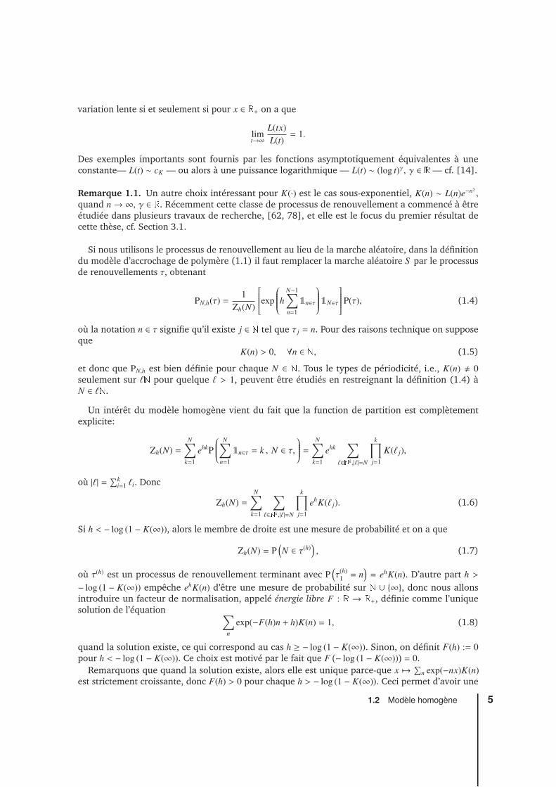
1 2 3 4J1= J2= J3= J =mt5 6

s s s s1 2 3 mtt1 t2 t3 tmt

Niccolò TorriThèse de doctorat

Numéro d’ordre : 114 - 2015 Année 2015

Université Claude Bernard Lyon 1Università degli Studi di Milano-Bicocca

École doctorale InfoMath, ED 512

Thèse de doctorat de l’Université de Lyonen cotutelle avec l’Università degli Studi di Milano-Bicocca /

Tesi di dottorato de l’Université de Lyonin cotutela con l’Università degli Studi di Milano-Bicocca

pour l’obtention du / per il conseguimento delDiplôme de Doctorat / Diploma di Dottorato di Ricerca

Spécialité : Mathématiques (Arrêté du 7 août 2006) / Specialità : Matematica


Soutenue publiquement le 18 Septembre 2015 par /Difesa pubblicamente il 18 Settembre 2015 da

Niccolò Torri

devant le Jury composé de:davanti alla commissione composta da:

Francesco CARAVENNA Università di Milano-Bicocca Directeur de thèse / Relatore di TesiFrancis COMETS Université Paris-Diderot Examinateur / EsaminatoreFranck DEN HOLLANDER University of Leiden Rapporteur / RefereeGiambattista GIACOMIN Université Paris-Diderot Président du Jury / Presidente commissioneNicolas PETERELIS Université de Nantes Examinateur / EsaminatoreChristophe SABOT Université Lyon 1 Examinateur / EsaminatoreFabio Lucio TONINELLI CNRS - Université Lyon 1 Directeur de thèse / Relatore di TesiNikolaos ZYGOURAS University of Warwick Rapporteur / Referee

Niccolò TorriPhénomènes de localisation et d’universalité pour des polymères aléatoires18 Septembre 2015Rapporteurs / Referee: Frank den Hollander , Nikolaos ZygourasDirecteurs de thèse / Relatori di tesi: Francesco Caravenna , Fabio Lucio Toninelli

Université Claude Bernard - Lyon 1équipe de Probabilités, statistique et physique mathématiqueInstitut Camille Jordan - UMR 5208Boulevard 18 Novembre 1918, Villeurbanne Cedex69622 , Lyon

Università degli Studi di Milano-BicoccaDipartimento di matematica e applicazioniVia Cozzi, 5520125 , Milano

AbstractA polymer is a long chain of repeated units (monomers) that are almost identical, but they can differin their degree of affinity for certain solvents. Such property allows to have interactions between thepolymer and the external environment. The environment has only a region that can interact withthe polymer. This interaction can attract or repel the polymer, by changing its spatial configuration,giving rise to localization and concentration phenomena. It is then possible to observe the existenceof a phase transition. Whenever such region is a point or a line (but also a plane or hyper-plane),then we talk about pinning model, which represents the main subject of this thesis.

From a mathematical point of view, the pinning model describes the behavior of a Markov chainin interaction with a distinguished state. This interaction can attract or repel the Markov chain pathwith a force tuned by two parameters, h and β. If β = 0 we obtain the homogeneous pinning model,which is completely solvable. The disordered pinning model, which corresponds to β > 0, is mostchallenging and mathematically interesting. In this case the interaction depends on an externalsource of randomness, independent of the Markov chain, called disorder. The interaction is realizedby perturbing the original Markov chain law via a Gibbs measure (which depends on the disorder,h and β), biasing the probability of a given path. Our main aim is to understand the structure of atypical Markov chain path under this new probability measure.

Pinning model with heavy-tailed disorder: The first research topic of this thesis is the pinningmodel in which the disorder is heavy-tailed and the return times of the Markov chain have a sub-exponential distribution. We prove that the set of the times at which the Markov chain visits thedistinguished state, suitably rescaled, converges in distribution to a limit random set which dependsonly on the disorder. We show that there exists a phase transition with a random critical point, βc(h),below which the limit set is trivial. This work has interesting connections with the directed polymerin random environment with heavy tail.

Critical behavior of the pinning model in the weak coupling regime: We consider a pinningmodel with a light-tailed disorder and the return times of the Markov chain with a polynomial taildistribution, with exponent tuned by α > 0. It is possible to show that there exists a non-trivialinteraction between the parameters h and β. Such interaction gives rise to a critical point, hc(β),depending only on the law of the disorder and of the Markov chain. If h > hc(β), then the Markovchain visits infinitely many times the distinguished state and we say that it is localized. Otherwise,if h < hc(β), then the Markov chain visits such state only a finite number of times. Therefore thecritical behavior of the model is deeply connected with the structure of hc(β). A very challengingproblem is to describe the behavior of the pinning model in the weak disorder regime. To be moreprecise, one wants to understand the behavior of the critical point, hc(β), when β→ 0. The answerdepends on the value of α: if it is smaller than 1/2, then there exists a value of β > 0 below which thecritical behavior of the model is the same of the homogeneous one. In this case we say that disorderis irrelevant. Otherwise, if α > 1/2, whatever be the value of β > 0, the disorder perturbs the Markovchain, and we say that disorder is relevant. In the case of 1/2 < α < 1, in the literature there arenon-matching estimates about the asymptotics of hc(β) as β→ 0. Getting the exact asymptotics forhc(β) represents the most important result of this thesis. We show that the behavior of the pinningmodel in the weak disorder limit is universal and the critical point, suitably rescaled, convergesto the related quantity of a continuum model. The proof is obtained by using a coarse-grainingprocedure, which generalizes the technique developed for the copolymer model, a relative polymermodel of the pinning one.

v

keywords: Pinning Model; Random Polymer; Directed Polymers; Weak Disorder; Scaling Limit;Disorder Relevance; Localization; Heavy Tails; Universality; Free Energy; Critical Point; Coarse-Graining

Résumé

D’un point de vue chimique et physique, un polymère est une chaîne d’unités répétées, appeléesmonomères, qui sont presque identiques, et chacune peut avoir un degré différent d’affinité aveccertains solvants. Cette caractéristique permet d’avoir des interactions entre le polymère et le milieudans lequel le polymère se trouve. Dans le milieu il y a une région interagissant, de manière attractiveou répulsive, avec le polymère. Cette interaction peut avoir un effet substantiel sur la structure dupolymère, en donnant lieu à des phénomènes de localisation et de concentration. Il est donc possibleobserver l’existence d’une transition de phase. Quand cette région est un point ou une ligne (oualors un plan ou un hyper-plan) on parle du modèle d’accrochage de polymère – pinning model –qui représente l’objet d’étude principal de cette thèse.

Mathématiquement le modèle d’accrochage de polymère décrit le comportement d’une chaînede Markov en interaction avec un état donné. Cette interaction peut attirer ou repousser le cheminde la chaîne de Markov avec une force modulée par deux paramètres, h et β. Quand β = 0 on parlede modèle homogène, qui est complètement solvable. Le modèle désordonné, qui correspond àβ > 0, est mathématiquement le plus intéressant. Dans ce cas l’interaction dépend d’une sourced’aléa extérieur indépendant de la chaîne de Markov, appelée désordre. L’interaction est réalisée enmodifiant la loi originelle de la chaîne de Markov par une mesure de Gibbs (dépendant du désordre,de h et de β), en changeant la probabilité d’une trajectoire donnée. La nouvelle probabilité obtenuedéfinit le modèle d’accrochage de polymère. Le but principal est d’étudier et de comprendre lastructure des trajectoires typiques de la chaîne de Markov sous cette nouvelle probabilité.

Modèle d’accrochage de polymère avec désordre à queues lourdes: Le premier sujet derecherche de cette thèse concerne le modèle d’accrochage de polymère où le désordre est à queueslourdes et où le temps de retour de la chaîne de Markov suit une distribution sous-exponentielle. Nousdémontrons que l’ensemble des temps dans lesquels la chaîne de Markov visite l’état donné, avecun opportun changement d’échelle, converge en loi vers un ensemble limite qui dépend seulementdu désordre. Nous démontrons qu’il existe une transition de phase avec un point critique aléatoire,βc(h), en dessous duquel l’ensemble limite est trivial. Ce travail a des connections intéressantes avecun autre modèle de polymère très répandu: le modèle de polymère dirigé en milieu aléatoire avecqueues lourdes.

Comportement critique du modèle d’accrochage de polymère dans la limite du désordrefaible: Nous étudions le modèle d’accrochage de polymère avec un désordre à queues légères et letemps de retour de la chaîne de Markov avec une distribution à queues polynomiales avec exposantcaractérisé par α > 0. Sous ces hypothèses on peut démontrer qu’il existe une interaction non-trivialeentre les paramètres h et β qui donne lieu à un point critique, hc(β), dépendant uniquement dela loi du désordre et de la chaîne de Markov. Si h > hc(β), alors la chaîne de Markov est localiséeautour de l’état donné et elle le visite un nombre infinie de fois. Autrement, si h < hc(β), la chaîne deMarkov visite l’état donné seulement un nombre fini de fois. Le comportement critique du modèle estdonc strictement lié à la structure de hc(β). Un problème très intéressant concerne le comportementdu modèle dans la limite du désordre faible. Plus précisément nous cherchons à comprendre lecomportement du point critique, hc(β), quand β→ 0. La réponse dépend de la valeur de α: si elle estplus petite de 1/2, alors il existe une valeur de β sous laquelle le comportement critique du modèleest le même que celui du modèle homogène associé. En revanche, si α > 1/2, quelque soit la valeurde β, le désordre perturbe la chaîne de Markov et nous disons qu’il y a pertinence du désordre. Dans

vi

le cas 1/2 < α < 1, dans la littérature on a des estimations sur l’asymptotique de hc(β) pour β → 0qui ne sont pas précises. Avoir trouvée l’asymptotique précise, c’est à dire un équivalent pour hc(β),représente le résultat le plus important de cette thèse. Précisément on montre que le comportementdu modèle d’accrochage de polymère dans la limite du désordre faible est universel et le pointcritique, opportunément changé d’échelle, converge vers la même quantité donnée par un modèlecontinu. La preuve est obtenue en utilisant une procédure de coarse-graining, qui généralise lestechniques utilisées pour des modèles des polymères proches de celui étudié dans cette thèse.

Sommario

Da un punto di vista chimico e fisico, un polimero è una catena di unità ripetute, chiamatemonomeri, quasi identiche nella struttura, ma che possono differire tra loro per il grado di affinitàrispetto ad alcuni solventi. Questa caratteristica permette di avere delle interazioni tra il polimero el’ambiente esterno in cui esso si trova. Nell’ambiente si trova una regione interagente, in manierapositiva o negativa, con il polimero. Questa interazione può avere un effetto sostanziale sullastrutture del polimero, dando luogo a fenomeni di localizzazione e concentrazione ed è dunquepossibile osservare l’esistenza di una transizione di fase. Nel caso in cui questa regione è un punto ouna linea (oppure un piano o un iper-piano) si parla di modello di pinning – pinning model –, cherappresenta il principale oggetto di studio di questa tesi.

Matematicamente il modello di pinning descrive il comportamento di una catena di Markovin interazione con uno suo stato dato. Questa interazione può attirare o respingere il camminodella catena di Markov con una forza modulata da due parametri, h e β. Quando β = 0 si parladi modello omogeneo, che è completamente risolubile. Il modello disordinato, che corrisponde aβ > 0, è matematicamente più interessante. In questo caso l’interazione dipende da una sorgentedi aleatorietà esterna, indipendente dalla catena di Markov, chiamata disordine. L’interazione èrealizzata modificando la legge originale della catena di Markov attraverso una misura di Gibbs(dipendente dal disordine, h e β), cambiando la probabilità di una traiettoria data. L’obiettivoprincipale è studiare e comprendere la struttura delle traiettorie tipiche della catena di Markovrispetto a questa nuova probabilità.

Modello di pinning con disordine a code pesanti: il primo lavoro di ricerca di questa tesiriguarda il modello di pinning in cui si considera un disordine a code pesanti e il tempo di ritornodella catena di Markov avente una distribuzione sotto-esponenziale. Noi dimostriamo che l’insiemedei tempi in cui la catena di Markov visita lo stato dato, opportunamente riscalato, converge inlegge verso un insieme limite, dipendente unicamente dal disordine. Dimostriamo inoltre che esisteuna transizione di fase con un punto critico aleatorio, βc(h), sotto il quale l’insieme limite è banale.Questo lavoro ha interessanti connessioni con un altro modello di polimeri molto studiato: il modellodi polimero diretto in ambiente aleatorio con code pesanti.

Comportamento critico del modello di pinning nel limite del disordine debole: In questosecondo lavoro consideriamo il modello di pinning con un disordine a code leggere e il tempo diritorno della catena di Markov con una distribuzione a code polinomiali con esponente caratterizzatoda α > 0. Sotto queste ipotesi si può dimostrare che esiste un’interazione non banale tra i parametrih e β che dà origine a un punto critico, hc(β), dipendente unicamente dalle leggi del disordine e dellacatena di Markov. Se h > hc(β), allora la catena di Markov è localizzata attorno allo stato dato e lovisita un numero infinito di volte. Altrimenti, se h < hc(β), la catena di Markov visita lo stato datosolamente un numero finito di volte. Il comportamento critico del modello è dunque profondamentelegato alla struttura di hc(β). Un problema molto interessante riguarda il comportamento del modellonel limite del disordine debole: più precisamente vogliamo comprendere il comportamento delpunto critico, hc(β), quando β → 0. La risposta dipende dal valore di α: se è più piccolo di 1/2,

vii

allora esiste un valore di β sotto il quale il comportamento critico del modello sarà lo stesso delmodello omogeneo associato. Altrimenti, se α > 1/2, qualunque sia il valore di β il disordine perturbala catena di Markov e diciamo che il disordine è rilevante. Nel caso 1/2 < α < 1, in letteraturanon esistono stime precise sull’asintotica di hc(β) quando β → 0. Aver trovato l’asintotica precisa,ovvero un equivalente per hc(β), rappresenta il risultato più importante di questa tesi. Precisamentedimostriamo che il comportamento del modello di pinning nel limite del disordine debole è universalee il punto critico, opportunamente riscalato, converge verso le rispettive quantità date da un modellocontinuo. La dimostrazione è ottenuta utilizzando una procedura di coarse-graining, che generalizzale tecniche utilizzate per dei modelli di polimero simili a quello studiato in questa tesi.

viii

Acknowledgements

I wish to thank all those who helped me in the realization of my Ph.D. thesis. I would like to thankmy advisors, Prof. Francesco Caravenna and Prof. Fabio Toninelli, for their support. They have beenfor me two mentors who taught me to do computations outside of the linearity of academic courses.

I thank Prof. Frank den Hollander and Prof. Nikolaos Zygouras for agreeing to be the refereesand evaluating my work. Moreover I thank the Professors Francis Comets, Giambattista Giacomin,Nicolas Pétrélis e Christophe Sabot for being part of my "jury de thèse".

I want to express my thanks to Prof. Giambattista Giacomin and Prof. Francesco Caravenna againto have given me, three years ago, the possibility to make my master thesis in Paris. Such experiencehas influenced my choice to (try to) stay in this country to pursue a Ph.D. Important supporters (inmany possible way) of such choice have been many friends and colleagues of the university, like,especially, Ilaria and Cristina. Without them I am not sure that this Ph.D. would started.

I have to be grateful to my family – Giancarla, Valter and Silvia – which has always supportedall my choices, as to all my (old and dear) friends Andrea C, Andrea G, Andrea M, Federico, Paco,Pietro, Marco.

Thanks to all colleagues of the Institut Camille Jordan and of the University of Milano–Bicocca forthe time spent together. In particular I would like to thank my Ph.D. colleagues with which I builtup something important also beside the academic world: Benoît, Luigia, Adriane, Blanche, Coline,Corentin, Élodie, François D, François V, Agathe, Mathias, Quentin, Thomas, Xiaolin, Fernando,Dario, Jacopo, Simone, Davide and Iman.

Finally I want to thank Camille, who made this last year and half special (and also her patience toreview and improve my french).

*Ce travail a été réalisé grâce au soutien financier du Programme Avenir Lyon Saint-Etienne de l’Université deLyon (ANR-11-IDEX-0007), dans le cadre du programme Investissements d’Avenir géré par l’Agence Nationalede la Recherche (ANR).

This work was supported by the Programme Avenir Lyon Saint-Etienne de l’Université de Lyon (ANR-11-IDEX-0007), within the program Investissements d’Avenir operated by the French National Research Agency(ANR).

ix

Contents

1 Polymères aléatoires 11.1 Modèle d’accrochage de polymère . . . . . . . . . . . . . . . . . . . . . . . . . . . . 21.2 Modèle homogène . . . . . . . . . . . . . . . . . . . . . . . . . . . . . . . . . . . . . 41.3 Modèle désordonné . . . . . . . . . . . . . . . . . . . . . . . . . . . . . . . . . . . . 7

1.3.1 Le critère de Harris . . . . . . . . . . . . . . . . . . . . . . . . . . . . . . . . 9

2 Polymers and probability 122.1 Pinning model . . . . . . . . . . . . . . . . . . . . . . . . . . . . . . . . . . . . . . . 142.2 Homogeneous pinning model . . . . . . . . . . . . . . . . . . . . . . . . . . . . . . . 152.3 Disordered pinning model . . . . . . . . . . . . . . . . . . . . . . . . . . . . . . . . . 20

2.3.1 The Harris criterion . . . . . . . . . . . . . . . . . . . . . . . . . . . . . . . . 222.3.2 The weak disorder regime . . . . . . . . . . . . . . . . . . . . . . . . . . . . 242.3.3 Universality in the weak coupling limit . . . . . . . . . . . . . . . . . . . . . 27

2.4 A related model: Directed polymers in a random environment . . . . . . . . . . . . . 282.4.1 The model . . . . . . . . . . . . . . . . . . . . . . . . . . . . . . . . . . . . . 282.4.2 Directed polymers in a random environment with finite exponential moments 292.4.3 Directed polymers in a random environment with heavy tails . . . . . . . . . 30

2.5 Random sets . . . . . . . . . . . . . . . . . . . . . . . . . . . . . . . . . . . . . . . . 332.5.1 Fell-Matheron topology . . . . . . . . . . . . . . . . . . . . . . . . . . . . . . 332.5.2 Characterization of random closed sets . . . . . . . . . . . . . . . . . . . . . 342.5.3 Renewal processes . . . . . . . . . . . . . . . . . . . . . . . . . . . . . . . . 352.5.4 Scaling limits of renewal processes: the Regenerative set . . . . . . . . . . . 362.5.5 Convergence of the pinning model . . . . . . . . . . . . . . . . . . . . . . . 37

3 Results of the Thesis 403.1 The Pinning Model with heavy tailed disorder . . . . . . . . . . . . . . . . . . . . . . 40

3.1.1 Definition of the model . . . . . . . . . . . . . . . . . . . . . . . . . . . . . . 403.1.2 Disorder and energy . . . . . . . . . . . . . . . . . . . . . . . . . . . . . . . 403.1.3 Renewal process and entropy . . . . . . . . . . . . . . . . . . . . . . . . . . 413.1.4 Main results . . . . . . . . . . . . . . . . . . . . . . . . . . . . . . . . . . . . 41

3.2 Universality for the pinning model in the weak coupling regime . . . . . . . . . . . . 433.2.1 General assumptions . . . . . . . . . . . . . . . . . . . . . . . . . . . . . . . 443.2.2 Main results . . . . . . . . . . . . . . . . . . . . . . . . . . . . . . . . . . . . 443.2.3 Further results . . . . . . . . . . . . . . . . . . . . . . . . . . . . . . . . . . 45

3.3 Conclusion and perspectives . . . . . . . . . . . . . . . . . . . . . . . . . . . . . . . 46

4 Pinning model with heavy-tailed disorder 494.1 Set-up and Results . . . . . . . . . . . . . . . . . . . . . . . . . . . . . . . . . . . . . 49

4.1.1 The Pinning Model . . . . . . . . . . . . . . . . . . . . . . . . . . . . . . . . 494.1.2 Main Results . . . . . . . . . . . . . . . . . . . . . . . . . . . . . . . . . . . . 504.1.3 Organization of the Chapter . . . . . . . . . . . . . . . . . . . . . . . . . . . 52

xi

4.2 Energy & entropy . . . . . . . . . . . . . . . . . . . . . . . . . . . . . . . . . . . . . 524.2.1 The Disorder . . . . . . . . . . . . . . . . . . . . . . . . . . . . . . . . . . . 534.2.2 The Energy . . . . . . . . . . . . . . . . . . . . . . . . . . . . . . . . . . . . 534.2.3 The entropy . . . . . . . . . . . . . . . . . . . . . . . . . . . . . . . . . . . . 554.2.4 The Energy-entropy . . . . . . . . . . . . . . . . . . . . . . . . . . . . . . . . 57

4.3 Convergence . . . . . . . . . . . . . . . . . . . . . . . . . . . . . . . . . . . . . . . . 584.3.1 Convergence Results . . . . . . . . . . . . . . . . . . . . . . . . . . . . . . . 584.3.2 Proof of theorem 4.5 . . . . . . . . . . . . . . . . . . . . . . . . . . . . . . . 62

4.4 Concentration . . . . . . . . . . . . . . . . . . . . . . . . . . . . . . . . . . . . . . . 634.4.1 General Setting of the Section . . . . . . . . . . . . . . . . . . . . . . . . . . 634.4.2 Proof of Theorem 4.4 . . . . . . . . . . . . . . . . . . . . . . . . . . . . . . . 634.4.3 Proof of Theorem 4.6 . . . . . . . . . . . . . . . . . . . . . . . . . . . . . . . 67

4.5 Proof of Theorem 4.7 . . . . . . . . . . . . . . . . . . . . . . . . . . . . . . . . . . . 674.6 The Directed polymer in random environment with heavy tails . . . . . . . . . . . . 69

4.6.1 The Structure of βc . . . . . . . . . . . . . . . . . . . . . . . . . . . . . . . . 704.A Asymptotic Behavior for Terminating Renewal Processes . . . . . . . . . . . . . . . . 71

4.A.1 The case of K(n) � e−cnγ

. . . . . . . . . . . . . . . . . . . . . . . . . . . . . . 72

5 Universality for the pinning model in the weak coupling regime 745.1 Introduction and motivation . . . . . . . . . . . . . . . . . . . . . . . . . . . . . . . 745.2 Main results . . . . . . . . . . . . . . . . . . . . . . . . . . . . . . . . . . . . . . . . 76

5.2.1 Pinning model revisited . . . . . . . . . . . . . . . . . . . . . . . . . . . . . 765.2.2 Free energy and critical curve . . . . . . . . . . . . . . . . . . . . . . . . . . 775.2.3 Main results . . . . . . . . . . . . . . . . . . . . . . . . . . . . . . . . . . . . 785.2.4 On the critical behavior . . . . . . . . . . . . . . . . . . . . . . . . . . . . . 805.2.5 Further results . . . . . . . . . . . . . . . . . . . . . . . . . . . . . . . . . . 805.2.6 Organization of the chapter . . . . . . . . . . . . . . . . . . . . . . . . . . . 82

5.3 Proof of Proposition 5.8 and Corollary 5.9 . . . . . . . . . . . . . . . . . . . . . . . . 825.3.1 Renewal results . . . . . . . . . . . . . . . . . . . . . . . . . . . . . . . . . . 825.3.2 Proof of relation (5.33) . . . . . . . . . . . . . . . . . . . . . . . . . . . . . . 855.3.3 Proof of (5.32), case p ≥ 0. . . . . . . . . . . . . . . . . . . . . . . . . . . . . 875.3.4 Proof of (5.32), case p ≤ 0. . . . . . . . . . . . . . . . . . . . . . . . . . . . . 87

5.4 Proof of Theorem 5.6 . . . . . . . . . . . . . . . . . . . . . . . . . . . . . . . . . . . 885.5 Proof of Theorem 5.4 . . . . . . . . . . . . . . . . . . . . . . . . . . . . . . . . . . . 91

5.5.1 Proof of relation (5.28) assuming (5.27) . . . . . . . . . . . . . . . . . . . . 925.5.2 Renewal process and regenerative set . . . . . . . . . . . . . . . . . . . . . . 925.5.3 Coarse-grained decomposition . . . . . . . . . . . . . . . . . . . . . . . . . . 935.5.4 General Strategy . . . . . . . . . . . . . . . . . . . . . . . . . . . . . . . . . 945.5.5 The coupling . . . . . . . . . . . . . . . . . . . . . . . . . . . . . . . . . . . 965.5.6 First step: f (1) ≺ f (2) . . . . . . . . . . . . . . . . . . . . . . . . . . . . . . . . 975.5.7 Second Step: f (2) ≺ f (3) . . . . . . . . . . . . . . . . . . . . . . . . . . . . . . 98

5.6 Proof of Theorem 5.3 . . . . . . . . . . . . . . . . . . . . . . . . . . . . . . . . . . . 1015.A Regenerative Set . . . . . . . . . . . . . . . . . . . . . . . . . . . . . . . . . . . . . . 101

5.A.1 Proof of Lemma 5.20 . . . . . . . . . . . . . . . . . . . . . . . . . . . . . . . 1015.A.2 Proof of Lemma 5.26 . . . . . . . . . . . . . . . . . . . . . . . . . . . . . . . 1035.A.3 Proof of Lemma 5.27 . . . . . . . . . . . . . . . . . . . . . . . . . . . . . . . 1055.A.4 Proof of Lemma 5.29 . . . . . . . . . . . . . . . . . . . . . . . . . . . . . . . 108

5.B Miscellanea . . . . . . . . . . . . . . . . . . . . . . . . . . . . . . . . . . . . . . . . . 1125.B.1 Proof of Lemma 5.12 . . . . . . . . . . . . . . . . . . . . . . . . . . . . . . . 1125.B.2 Proof of Proposition 5.13 . . . . . . . . . . . . . . . . . . . . . . . . . . . . . 113

6 Continuum Free Energy, Proof Theorem 3.7 114

xii

6.1 Modified partition function . . . . . . . . . . . . . . . . . . . . . . . . . . . . . . . 1146.2 Existence of the Free Energy, conditioned case . . . . . . . . . . . . . . . . . . . . . 1176.3 Existence of the Free Energy, free case . . . . . . . . . . . . . . . . . . . . . . . . . . 120

Bibliography 127

xiii

1Polymères aléatoires

Le sujet principal de cette thèse concerne les polymères aléatoires. Un polymère est une longuemolécule linéaire formée par une chaîne d’unités répétées appelées monomères. La définitionmoderne de polymère a été proposée en 1920 par le chimiste Hermann Staudinger (Prix Nobelde chimie en 1953), qui démontra pour la première fois l’existence de macromolécules organiséesdans une structure de chaîne linéaire. Dans la définition IUPAC (International Union of Pure andApplied Chemistry) actuelle [55], un polymère est une substance composée de macromolécules.Une macromolécule est une molécule de masse moléculaire relative élevée et sa structure estessentiellement donnée par la répétition de molécules avec une petite masse moléculaire relative.Ces unités sont appelées monomères.

On peut classifier les polymères dans deux grandes familles:

• homo-polymères Un polymère avec un seul type de monomères. Les exemples communssont donnés par les matières plastiques, comme le polyethylene terephthalate (utilisé dans lafabrication des bouteilles en plastique).

• co-polymère Un polymère avec plusieurs types de monomères. Des exemples, l’ADN et l’ARN.

L’organisation dans l’espace du polymère est très complexe, avec des auto-interactions entredifférents portions de la chaîne et des interactions externes avec l’environnement dans lequelle polymère se trouve. L’interaction avec l’environnement dépend du degré d’affinité de chaquemonomère et de leur position dans la chaîne. Un exemple de cette complexité est évidente dansla Bovine spongiform encephalopathy (BSE), communément appelé maladie de la vache folle. Danscette maladie neurodégénérative des protéines situées dans les cellules neuronales changent leurstructure géométrique. Ce changement conduit à une modification de leur propriétés chimiques quiforce une agrégation non-naturel, induisant la mort des cellules neuronales.

Plusieurs efforts de recherche sont concentrés sur la description et la prédiction du comportementd’un polymère en interaction avec un environnement externe. Ce sujet a dépassé les sciences expéri-mentales, devenant un important sujet de recherche en physique théorique et en mathématiques,introduisant le concept de polymère abstrait. L’analyse rigoureuse des propriétés mathématiques despolymères abstraits est un domaine de recherche actif dans la physique mathématique et des progrèsimportants ont été réalisés dans les dernières années, voir, e.g., les monographies [31, 21, 44, 45] etl’article de revue [38].

Pour comprendre le concept de polymère abstrait on peut essayer à trouver une réponse à la(fondamentale) question

Quelle est la façon mathématique la plus simple pour modéliser un polymère?L’idée est d’introduire un modèle simplifié, qui peut décrire la nature essentielle du phénomène

observé, conduisant à la compréhension des mécanismes de base. De plus, si on veut faire desmathématiques, on ne peut pas être trop loin de modèles super-simplifiés. Nous approchons leproblème en regardant le polymère en interaction avec l’environnement externe comme un système(la chaîne du polymère) perturbé par un champ externe (l’environnement) afin d’utiliser les principesde la mécanique statistique pour comprendre les effets de l’environnement sur le polymère. Cesprincipes suggèrent d’introduire une classe de modèles mathématiques basés sur les marchesaléatoires et plus précisément les marches aléatoires auto-évitant: un incrément correspond à unmonomère du polymère et une réalisation de la marche représente une configuration spatiale(ou trajectoire) du polymère. La contrainte "auto-évitante" décrit le fait que deux monomères nepeuvent pas occuper la même position dans l’espace. En ce sens un polymère abstrait est unetrajectoire de marche aléatoire sur un graphe donné, comme �2, �3 ou, plus généralement, �d. Lesmarches aléatoires auto-évitante sont des modèles extrêmement difficiles et ils présentent encore de

1

nombreuses questions ouvertes [64]. Les modèles de polymère beaucoup plus traitables, satisfaisantla contrainte auto-évitante, sont basés sur les marches aléatoires dirigées. Ces sont tout simplementdes marche aléatoires dans lesquels une composante est déterministe et strictement croissante,i.e., (n, S n)n∈�, où S = (S n)n∈� est une marche aléatoire sur �d−1. Ce choix permet d’éviter certainsproblèmes techniques, comme la présence des spirales – dead-loops – dans les trajectoires de lamarche aléatoire.

Une fois introduit le polymère, il faut définir l’environnement et sa manière d’interagir avec lepolymère. Considérons une situation réelle, dans laquelle il y a un polymère en interaction avecune membrane pénétrable (ou impénétrable). Imaginons que chaque monomère a un degré donnéd’affinité avec la membrane, qui peut être positif ou négatif. Une affinité positive correspond aufait que le monomère est attiré par la membrane et donc il aura tendance à se localiser autourd’elle. Au contraire, une affinité négative signifie qu’il est repoussé. Pour comprendre si la chaîneest localisé ou de-localisé autour de la membrane, nous devons connaître la fraction de monomèresavec des interactions positives/négatives et leur placement dans la chaîne. Pour construire unmodèle pour décrire ces interactions on peut idéaliser la membrane comme une région donnéede l’espace, par exemple une ligne ou un plan, et à chaque fois que la marche aléatoire traversecette région d’interaction, elle reçoit une récompense/pénalité donnée par le site de contact. Cesrécompenses/pénalités perturbent la trajectoire de marche aléatoire, donnant lieu à des phénomènesde localisation/de-localisation. Mathématiquement, la localisation signifie que la marche aléatoire(n, S n)n∈� a un densité d’intersections positives avec la membrane, voir Figure 2.1.

Pour étudier les interactions entre le polymère et la membrane il suffit de connaître les sitesde contact entre eux. Nous pouvons aller au-delà des modèles de marches aléatoires dirigées enconsidérant des processus de contact plus généraux, qui sont les processus de renouvellement [6, 37]et le modèle de polymère associé est appelé modèle d’accrochage de polymère (pinning model). Cettegénéralisation permet, par exemple, de décrire une grande classe d’interactions entre différentspolymères, comme l’ADN. L’ADN est une longue molécule composée d’une double-hélice de deuxpolymères collés ensemble par des liaisons chimiques. Dans la Section 2.2 nous décrivons un modèlebasé sur le processus de renouvellement qui décrit la dénaturation de l’ADN, i.e., le processuschimique qui permet la séparation de la double-hélice. Typiquement la dénaturation de l’ADNdépende de certains facteurs extérieurs, comme la température: des températures élevées induisentle processus de dénaturation de l’ADN, tandis que des basses températures favorisent une situationoù la double-hélice est liée. De plus, il existe une température critique au-dessus de laquelle on a ladénaturation de l’ADN. Pour introduire ce modèle, nous idéalisons l’ADN comme une alternancede chemins rectilignes, correspondant aux parties où la double-hélice est liée, et des boucles, où ladouble-hélice est ouverte. Un processus de renouvellement bien choisi donne les points où l’hélicese divise, donnant lieu à les boucles. La formation d’une boucle est réglée par un coefficient T quidécrit la température du système. Les interactions entre les différentes parties de la chaîne et, plusgénéralement, tous les détails concernant l’ADN réel, comme la composition chimique, la torsion,sont ignorés. Ce modèle a été introduit par Poland et Scheraga [71] et il est un des premiers modèlesd’ADN qui ont fourni l’existence d’une température critique Tc qui divise le régime liée de celuidénaturée.

1.1 Modèle d’accrochage de polymèreLe modèle d’accrochage de polymère représente le sujet central de cette thèse. Dans ce modèle

on fixe une marche aléatoire S = (S n)n∈� ⊂ � et un nombre N ∈ �. Une trajectoire du polymèreabstrait est donnée par une interpolation linéaire des points (n, S n)n≤N , qui est le graphe d’unemarche aléatoire dirigée de longueur N. Nous fixons une région d’interaction dans l’espace, commeune ligne, et dans le cas le plus simple (le homogène), cf. Section 1.2, à chaque fois que la marchealéatoire visite cette région, elle reçoit une récompense constante, positive ou négative, h ∈ �, quiattire ou repousse la marche aléatoire de la région. On peut penser que si la récompense est positive,

2 Chapter 1 Polymères aléatoires

alors le polymère a une affinité positive avec cette région.

Si la région est précisément l’axe x, le fait que (n, S n)n∈� touche la ligne équivaut à considérerla seule marche aléatoire (S n)n∈� en lui donnant une récompense/pénalité à chaque fois qu’ellevisite l’état 0. Si nous choisissons une ligne horizontale différente, alors nous changeons l’état aveclequel la marche aléatoire a une interaction privilégiée. Les récompenses/pénalités sont donnéesen changeant la probabilité d’une trajectoire donnée jusqu’à N: à chaque n ≤ N, nous donnons unpoids exponentiel exp(h), h ∈ � à la probabilité que S n = 0. Par conséquent des valeurs positives de hpoussent les chemins de la marche aléatoire à visiter souvent 0, tandis que les valeurs négatives de hdécouragent ces visites. Une fois fixée la marche aléatoire S , il est possible de prouver qu’il existeune valeur critique, hc tel que, pour h > hc, elle devient récurrent positive, en visitant 0 un nombreinfinie de fois, et pour h < hc la marche aléatoire est transiente, en visitant 0 au plus un numéro finide fois. Dans le langage des polymères cette discussion signifie qu’il existe une valeur critique dehc qui divise un comportement localisé d’un de-localisé. La valeur critique hc est déterminée par laloi originelle de la marche aléatoire: par exemple, si S est le marche aléatoire simple, hc = 0, sinon,si S est une marche aléatoire simple non-symétrique, i.e., P(X1 = 1) = p, P(X1 = −1) = 1 − p, avecp � 1/2, alors hc > 0 et sa valeur dépend de la différence entre p et 1/2.

Le cas dans lequel les récompenses ne sont pas homogènes est le plus difficile et mathématiquementle plus intéressant. Il est appelé modèle d’accrochage de polymère désordonné, nous parlerons dansla Section 1.3. Dans ce cas, nous introduisons un désordre ω = (ωi)i∈� et les récompenses seront sousla forme exp(βωn + h), où β ∈ �+. L’idée est que ωn représente l’affinité entre la région d’interactionet le n-ième monomère. Lassez-nous remarquer que le modèle désordonné est une perturbationdu modèle homogène, et la perturbation dépend d’un facteur β. Nous générons le désordre d’unemanière aléatoire, i.e., le désordre est une réalisation gelée d’une suite aléatoire ω = (ωi)i∈�. Uneréalisation donnée correspond à un polymère spécifique et la loi de la séquence aléatoire décritune famille de polymères. Différents choix de la loi du désordre conduisent à des comportementsdifférents du modèle d’accrochage de polymère. Le cas le plus simple est quand le désordre décritseulement si un monomère a une affinité positive ou négative avec la région d’interaction – l’état 0 –,i.e., quand ωi ∈ {−1,+1}. Un autre cas très important est le cas Gaussien, où nous précisons aussi ledegré d’affinité de chaque monomère. En général, les cas les plus étudiés ne vont pas plus loin queces deux [44, 45, 31]. Dans cette thèse, nous concentrons notre attention sur le cas où le désordreest très hétérogène, ce qui signifie mathématiquement que la fonction de distribution de ωi a unequeue lourde, cf. Section 3.1.

Pour comprendre le comportement du modèle d’accrochage de polymère désordonné, nousintroduisons le concept de compétition énergie-entropie: l’énergie est donnée par la somme totaledes récompenses, et l’entropie est le coût associé à la configuration spatiale du polymère: plus uneconfiguration est atypique, plus le coût de l’entropie est élevé. De cette manière, les configurationsatypiques peuvent devenir typique pour le polymère si l’énergie gagnée bat le coût entropiqueassocié. Si on suppose que le désordre a des moments exponentiels finis, nous pouvons prouverl’existence d’un point critique hc(β), qui sépare le comportement récurrent positif du comportementtransiente de la marche aléatoire. Selon les observations qualitatives faites ci-dessus, si β est grand,alors hc(β) sera différent du point critique d’un modèle homogène. En revanche, si β est très petit,alors la présence du désordre et son influence sur le point critique hc(β) dépend de la structure de lamarche aléatoire.

Quand l’introduction d’une quantité arbitrairement petite de désordre modifie le point critiquenous parlons de pertinence du désordre et dans ce cas un problème ouvert et intéressant consiste àtrouver l’asymptotique exacte de hc(β) quand β→ 0. Le résultat le plus important de cette thèse estla solution à ce problème, cf. Section 3.2.

1.1 Modèle d’accrochage de polymère 3

1.2 Modèle homogènePour introduire le modèle d’accrochage de polymère homogène, nous considérons une marche

aléatoire simple (S = (S n)n∈�,P) sur �, i.e. S n =∑n

i=1 Xi où Xi ∈ {−1, 1} et P(Xi = −1) = P(Xi = 1) = 1/2.La marche aléatoire dirigée associée est le processus (n, S n)n∈�, qui décrit la configuration du polymèredans l’espace. Dans ce modèle homogène pour N ∈ � fixé nous modifions la loi de la marche aléatoireà lui donnant une récompense/pénalité à chaque fois qu’elle visite 0 avant N. Plus précisément, S n

peut visiter 0 seulement quand n est pair, donc pour chaque N ∈ 2� nous introduisons la famille deprobabilités PN,h indexes par h ∈ � définie comme

PN,h(S ) =1

Zh(N)

⎡⎢⎢⎢⎢⎢⎣exp

⎛⎜⎜⎜⎜⎜⎝hN∑

n=1

1S n=0

⎞⎟⎟⎟⎟⎟⎠1S N=0

⎤⎥⎥⎥⎥⎥⎦P(S ) (1.1)

La constante de normalisation Zh(N) est appelée fonction de partition. Remarquons que si on permetà Xi de prendre la valeur 0, i.e. Xi ∈ {−1, 0, 1}, alors la restriction N ∈ 2� n’est pas nécessaire.

Pour définir (1.1) il suffi de connaître la sequence des temps τ = {τ0 = 0, τ1, τ2, · · · } auxquels lamarche aléatoire visite 0, i.e.,

τ0 = 0,τk = inf{i > τk−1 : S i = 0}.

Pour la propriété de Markov, la suite (τi − τi−1)i∈� est i.i.d. sous P et un tel processus est appeléprocessus de renouvellement [6, 37]. La loi du processus de renouvellement est caractérisée par la loide τ1

K(n) = P(τ1 = n). (1.2)

Les exemples plus généraux de processus de renouvellement sont fournis par le temps de retourà zéro des chaînes de Markov discrètes. D’autre part, si nous considérons un processus de renou-vellement τ, alors on peut vérifier que An = n − sup{τk : τk ≤ n} est une chaîne de Markov avec sonensemble de niveau zéro, {n ∈ �0 : An = 0}, qui est donné par τ. Cette dualité entre les processus derenouvellement et les chaînes de Markov est représentée en Figure 2.2.

Remarquons que dans le cas de la marche aléatoire simple et symétrique la formule de Stirlingfournit l’asymptotique de K(2n), voir e.g. [44, Appendix A.6]:

K(2n) = P(τ1 = 2n) = P (S 2n = 0, S 1 � 0, · · · , S 2n−1 � 0) ∼n→∞

√1

4π1

n3/2 .

En particulier on en déduit que l’état 0 est récurrent pour la marche aléatoire simple et symétrique.D’autre part, pour une marche aléatoire simple mais non-symétrique, i.e., P(X1 = 1) = p, P(X1 =

−1) = 1 − p, p � 1/2, le même genre d’estimation fournit P(τ1 < ∞) < 1, ce qui signifie que la marchealéatoire est transiente. Ceci motive le fait que pour un processus de renouvellement général, K(·)est une probabilité sur � ∪ {∞}, avec K(∞) := 1 −

∑n∈� K(n) ≥ 0. À Chaque fois que K(∞) > 0, on dit

que le processus de renouvellement τ est terminant. Ceci est équivalent à dire que p.s. τ est donnépar un nombre fini de points. La classe de processus de renouvellement considérée dans cette sectiongénéralise le cas de la marche aléatoire simple. Cette famille est indexée par un exposant α > 0, quicontrôle le comportement polynomial de K(·)

K(n) ∼L(n)n1+α , n→ ∞, (1.3)

où L(·) est une function à variation lente. Nous rappelons que L : �+ → �+ est une function à


variation lente si et seulement si pour x ∈ �+ on a que

limt→∞

L(tx)L(t)

= 1.

Des exemples importants sont fournis par les fonctions asymptotiquement équivalentes à uneconstante— L(t) ∼ cK — ou alors à une puissance logarithmique — L(t) ∼ (log t)γ, γ ∈ � — cf. [14].

Remarque 1.1. Un autre choix intéressant pour K(·) est le cas sous-exponentiel, K(n) ∼ L(n)e−nγ ,quand n→ ∞, γ ∈ �. Récemment cette classe de processus de renouvellement a commencé à êtreétudiée dans plusieurs travaux de recherche, [62, 78], et elle est le focus du premier résultat decette thèse, cf. Section 3.1.

Si nous utilisons le processus de renouvellement au lieu de la marche aléatoire, dans la définitiondu modèle d’accrochage de polymère (1.1) il faut remplacer la marche aléatoire S par le processusde renouvellements τ, obtenant

PN,h(τ) =1

Zh(N)

⎡⎢⎢⎢⎢⎢⎢⎣exp

⎛⎜⎜⎜⎜⎜⎜⎝hN−1∑n=1

1n∈τ

⎞⎟⎟⎟⎟⎟⎟⎠1N∈τ

⎤⎥⎥⎥⎥⎥⎥⎦P(τ), (1.4)

où la notation n ∈ τ signifie qu’il existe j ∈ � tel que τ j = n. Pour des raisons technique on supposeque

K(n) > 0, ∀n ∈ �, (1.5)

et donc que PN,h est bien définie pour chaque N ∈ �. Tous le types de périodicité, i.e., K(n) � 0seulement sur �� pour quelque � > 1, peuvent être étudiés en restreignant la définition (1.4) àN ∈ ��.

Un intérêt du modèle homogène vient du fait que la function de partition est complètementexplicite:

Zh(N) =N∑

k=1

ehkP

⎛⎜⎜⎜⎜⎜⎝N∑

n=1

1n∈τ = k , N ∈ τ,⎞⎟⎟⎟⎟⎟⎠ =

N∑k=1

ehk∑

�∈�k ,|�|=N

k∏j=1

K(� j),

où |�| =∑k

i=1 �i. Donc

Zh(N) =N∑

k=1

∑�∈�k ,|�|=N

k∏j=1

ehK(� j). (1.6)

Si h < − log (1 − K(∞)), alors le membre de droite est une mesure de probabilité et on a que

Zh(N) = P(N ∈ τ(h)

), (1.7)

où τ(h) est un processus de renouvellement terminant avec P(τ(h)

1 = n)= ehK(n). D’autre part h >

− log (1 − K(∞)) empêche ehK(n) d’être une mesure de probabilité sur � ∪ {∞}, donc nous allonsintroduire un facteur de normalisation, appelé énergie libre F : � → �+, définie comme l’uniquesolution de l’équation ∑

n

exp(−F(h)n + h)K(n) = 1, (1.8)

quand la solution existe, ce qui correspond au cas h ≥ − log (1 − K(∞)). Sinon, on définit F(h) := 0pour h < − log (1 − K(∞)). Ce choix est motivé par le fait que F

(− log (1 − K(∞))

)= 0.

Remarquons que quand la solution existe, alors elle est unique parce-que x �→∑

n exp(−nx)K(n)est strictement croissante, donc F(h) > 0 pour chaque h > − log (1 − K(∞)). Ceci permet d’avoir une

1.2 Modèle homogène 5

forme générale de la fonction de partition:

Zh(N) = eNF(h)P(N ∈ τ(h)

), (1.9)

où τ(h) est un processus de renouvellement tel que

P(τ(h)

1 = n)= exp(−F(h)n + h)K(n). (1.10)

Notons que si h < − log (1 − K(∞)), alors (1.9) est exactement (1.7).Pour résumer, le modèle homogène PN,h est toujours la loi d’un processus de renouvellement

conditionné à visiter N et (1.4) peut être écrit de la manière suivante: pour chaque 0 ≤ �1 < · · · <�n = N, �i ∈ �

PN,h(τ1 = �1, · · · , τn = �n) = P(τ(h)

1 = �1, · · · , τ(h)n = �n

∣∣∣N ∈ τ(h)), (1.11)

où τ(h) est le processus de renouvellement introduit en (1.9). De plus il existe une valeur critique deh

hc = − log (1 − K(∞)) (1.12)

telle que, si h < hc, alors τ est terminant, et si h > hc non-terminant. Nous pouvons aller au-delà dece résultat, en donnant une estimation quantitative sur la fraction de points de τ dans [0,N], i.e.,1N∑N

n=1 1n∈τ: si h > hc, alors la loi de τ1 est e−F(h)n+hK(n), qui a une espérance finie, et donc la distanceentre deux points consécutifs est finite. On peut conclure que {τ ∩ [0,N]} ≈ mh N, pour quelquemh > 0. D’autre part si h < hc, alors le processus de renouvellement est terminant, et donc il n’y aqu’un nombre fini de points dans �. Ceci suggère que {τ ∩ [0,N]} = o(N), quand N → ∞. Ce résultatpeut être rendu rigoureux: nous observons que

EN,h

⎡⎢⎢⎢⎢⎢⎣ 1N

N∑n=1

1n∈τ

⎤⎥⎥⎥⎥⎥⎦ = ddh

1N

log Zh(N) (1.13)

et que

F(h) = limN→∞

1N

log Zh(N). (1.14)

Un argument de convexité assure que nous pouvons échanger la dérivée par rapport à h avec lalimite N → ∞, pour obtenir

F′(h) = limN→∞

ddh

1N

log Zh(N) = limN→∞

EN,h

⎡⎢⎢⎢⎢⎢⎣ 1N

N∑n=1

1n∈τ

⎤⎥⎥⎥⎥⎥⎦ . (1.15)

En particulier F′(h) > 0 si h > − log (1 − K(∞)), et il est égal à 0 si h < − log (1 − K(∞)).

Remarque 1.2. Pour démontrer (1.14), nous considérons Zh(N) écrit comme en (1.9) et nousmontrons que si h ∈ �, alors la function P

(N ∈ τ(h)

)décroît polynomialement quand N → ∞. Ce

résultat est conséquence du Théorème (2.82) et (2.85). Pour une preuve détaillée voir, e.g., [44,Proposition 1.1].

Ce résultat peut être formulé comme la convergence en probabilité de 1N∑N

n=1 1n∈τ vers F′(h), cf.[45, Proposition 2.9]

Théorème 1.1. Pour tout ε > 0

limN→∞

PN,h

⎛⎜⎜⎜⎜⎜⎝∣∣∣∣∣∣∣1N

N∑n=1

1n∈τ − F′(h)

∣∣∣∣∣∣∣ ≤ ε⎞⎟⎟⎟⎟⎟⎠ = 1. (1.16)

De plus F′(h) = 0 si h < − log (1 − K(∞)), tandis que, si h > − log (1 − K(∞)), F′(h) > 0.


Une fois que nous avons identifié la valeur critique hc, qui définit la transition de phase pourle modèle homogène, nous pouvons considérer l’interaction entre cette transition de phase et lecomportement critique de l’énergie libre, c’est-à-dire la régularité de F(h) quand h ↓ hc. Dans ce butnous regardons le comportement asymptotique de Ψ(x) = 1 −

∑n∈� e−xnK(n) quand x→ 0. Détaillons

ce calcul dans le cas où K(·) est une mesure de probabilité sur � satisfaisant (1.3), avec L(n) égal àune constante cK , et (1.5). Dans ce cas hc = 0 et

Ψ(x) = 1 −∞∑

n=1

e−xnK(n) = 1 −∞∑

n=1

e−xn

⎛⎜⎜⎜⎜⎜⎜⎝∑j≥n

K( j) −∑

j≥n+1

K( j)

⎞⎟⎟⎟⎟⎟⎟⎠=

⎛⎜⎜⎜⎜⎜⎜⎝∑j≥1

K( j) +∞∑

n=1

e−xn∑

j≥n+1

K( j)

⎞⎟⎟⎟⎟⎟⎟⎠ −∞∑

n=1

e−xn∑j≥n

K( j)

=(1 − e−x)∞∑

n=0

⎛⎜⎜⎜⎜⎜⎜⎝∑

j≥n+1

K( j)

⎞⎟⎟⎟⎟⎟⎟⎠ e−xn.

Si α > 1 on a immédiatementΨ(x) ∼

x→0xE [τ1] , (1.17)

et si α ∈ (0, 1) une approximation en sommes de Riemann sum donne

Ψ(x) ∼x→0

x∑

n

cK

αnαe−xn ∼

x→0

cK xα

α

∞∫0

s−αe−sds = cKΓ(1 − α)α

xα. (1.18)

En rappelant que Ψ(F(h)) = 1 − eh, et en inversant les asymptotique dans les expressions (1.17)et (1.18), on obtiene le comportement critique de F(h). Le résultat précis et général est dans [44,Theorem 2.1]:

Théorème 1.2. Pour tout α ≥ 0 et L(·) satisfaisant (1.3), il existe une unique fonction à variation lenteL(·) telle que

F(h) h↘hc∼ (h − hc)1/min{α,1}L (1/(h − hc)) . (1.19)

En particulier L(·) est une constante si α > 1.

Comme conséquence de ce théorème nous avons que si α > 1, alors F(h) n’est pas C1 au pointcritique et nous disons que la transition est du premier ordre. En générale on dit que le modèleprésente une transition de phase de ordre k si F(h) est Ck−1 mais pas Ck au point critique. Le modèlehomogène a une transition de phase de ordre k, k = 2, 3, · · · , à h = hc si α ∈ [1/k, 1/(k − 1)).

1.3 Modèle désordonnéLe Modèle d’accrochage de polymère désordonné est défini comme une perturbation aléatoire du

modèle homogène (1.4). Pour chaque i, i = 1, · · · ,N, nous remplaçons l’exposant h par βωi + h, où ωi

est une valeur donnée (gelée), indépendante du processus de renouvellement. La suite ω = (ωi)i∈�est appelée désordre du système et elle est une réalisation d’une sequence aléatoire donnée – gelée.Nous notons � sa loi.

Pour N ∈ � nous considérerons la famille de mesures de probabilité PωN,h,β, indexée par h ∈ �,β ∈ �+ définie comme

PωN,h,β(τ) =1

Zωβ,h(N)

⎡⎢⎢⎢⎢⎢⎣exp

⎛⎜⎜⎜⎜⎜⎝N∑

n=1

(βωn + h)1N∈τ

⎞⎟⎟⎟⎟⎟⎠1n∈τ

⎤⎥⎥⎥⎥⎥⎦P(τ). (1.20)

Dés lors que ω est une réalisation fixée, nous appelons (1.22) le modèle gelé (quenched).

1.3 Modèle désordonné 7

Nous supposons que la suite aléatoire ω est i.i.d. avec des moments exponentiels finis. De plus, ω1est de moyenne nulle, de variance unitaire et il existe β0 > 0 tel que

Λ(β) = log�[eβω1 ] < ∞ ∀β ∈ (−β0, β0), �[ω1] = 0, �[ω1] = 1. (1.21)

Sous ces hypothèses il est utile de faire le changement de paramétre h �→ h − Λ(β), pour normaliserla variable eβω1 et nous re-définissons (1.20) comme

PωN,h,β(τ) =1

Zωβ,h(N)

⎡⎢⎢⎢⎢⎢⎣exp

⎛⎜⎜⎜⎜⎜⎝N∑

n=1

(βωn − Λ(β) + h)1n∈τ

⎞⎟⎟⎟⎟⎟⎠1n∈τ

⎤⎥⎥⎥⎥⎥⎦P(τ). (1.22)

Remarque 1.3. L’hypothèse sur les moments exponentiels est très importante pour les résultats quenous allons présenter dans la suite, et des choix différents de désordre fournissent un comportementtrès différent pour le modèle d’accrochage de polymère. Ceci est, par exemple, le cas de variablesaléatoires à queue lourde que nous discutons dans la Section 3.1.

Par analogie avec le modèle homogène nous étudions le comportement du modèle d’accrochagede polymère par l’analyse de l’énergie libre, définie comme

F(β, h) = limN→∞

1N�

[log Zωβ,h(N)

], (1.23)

où la fonction de partition Zωβ,h(N) a été introduit en (1.22). L’existence de l’énergie libre décent d’un

argument de super-additivité. Le résultat peut-être amélioré en utilisant le théorème ergotique deKingman [58], qui assure la convergence p.s. du membre de droit, c’est-à-dire


1N

log Zωβ,h(N), � − a.s.

Voir e.g. [44, Chapter 4].

Pour étudier les propriétés critiques du modèle d’accrochage de polymère désordonné nouscommençons par noter que le modèle d’accrochage de polymère homogènes fournit des limitesinférieures et supérieures pour l’énergie libre:

F(0, h − Λ(β)) ≤ F(β, h) ≤ F(0, h). (1.24)

En particule, on a que F(β, h) ≥ 0, parce-que l’énergie libre du modèle homogène est positive.L’inégalité de droit, F(β, h) ≤ F(0, h), est une conséquence immédiat de l’inégalité de Jensen et elleest appelée borne annealed. L’inégalité de Jensen fournit aussi la preuve de l’inégalité de gauche:

log Zβ,h(N) = log EN,h−Λ(β)

[e∑N

n=1 βωn1n∈�]+ log ZN,h−Λ(β)

≥N∑

n=1

βωnPN,h−Λ(β)(τ1 = N) + log ZN,h−Λ(β),

où EN,h−Λ(β) est l’espérance du modèle homogène de paramètre h − Λ(β). En prenant l’espérance parrapport au désordre � on obtient le le résultat, car � [ωn] = 0.

Nous remarquons que pour chaque β > 0 la function h �→ F(β, h) est monotone et donc le pointcritique

hc(β) := sup{h : F(β, h) = 0} (1.25)

est bien définie et divise le plan (h, β) à deux régions L = {(β, h) : F(β, h) > 0} and D = {(β, h) :F(β, h) = 0}. On peut prouver, pour le modèle désordonné, une version analogue du Théorème 1.1


(cf. les monographies [44, 31, 45].):

(β, h) ∈ L ⇔ ∃mβ,h > 0 : ∀ ε > 0 PωN,h,β

⎛⎜⎜⎜⎜⎜⎝∣∣∣∣∣∣∣1N

N∑n=1

1n∈τ − mβ,h

∣∣∣∣∣∣∣ ≤ ε⎞⎟⎟⎟⎟⎟⎠ �−probability

→N→∞

1,

(1.26)

(β, h) ∈◦D ⇔ : ∀ ε > 0 PωN,h,β

⎛⎜⎜⎜⎜⎜⎝∣∣∣∣∣∣∣1N

N∑n=1

1n∈τ

∣∣∣∣∣∣∣ ≤ ε⎞⎟⎟⎟⎟⎟⎠ �−probability

→N→∞

1.

De plus (1.24) donnehc(0) ≤ hc(β) ≤ hc(0) + Λ(β) (1.27)

et hc(0) est la valeur critique annealed. Nous rappelons que hc(0) = − log (1 − K(∞)). Il est maintenantnaturel de se demander si la présence du désordre joue un rôle ou non. Une prédiction heuristique,mais précise, est donnée par le critère de Harris [51] et Figure 2.3.

1.3.1 Le critère de HarrisLe critère de Harris a été proposé dans les années 70 pour comprendre si et comment l’introduction

d’une petite quantité de désordre dans un modèle homogène peut changer son comportement critique.Dans l’article original [51] seul le modèle d’Ising dilué est considéré, mais les idées développéessont très utiles pour comprendre la présence du désordre dans de nombreux modèles désordonnés,parmi lesquels on retrouve le modèle d’accrochage de polymère. Dans ce dernier cas, ce critère ainspiré différentes méthodes pour comprendre quand le désordre ω perturbe le comportement dumodèle, c’est-à-dire quand les propriétés critiques du système sont différentes de celles d’un modèleannealed [33, 40]. Le modèle annealed est un type particulier de modèle homogène, cf. (1.28). Ceque nous entendons par propriété critique concerne le comportement du modèle à proximité dupoint critique, i.e., quand h ≈ hc(β). En particulier un des nos buts est de décrire comment F(β, h)converge vers 0 quand h ↘ hc(β), en comparant l’exposant critique du modèle désordonné avecl’exposant critique du modèle annealed, (qui est le même que celui du modèle homogène, cf. (1.19)).Chaque fois que l’exposant critique du modèle désordonné est différente de celui homogène, mêmesi β est arbitrairement petit, nous disons qu’il y a pertinence du désordre.

Dans le cas du modèle d’accrochage de polymère l’analyse de l’exposant critique est strictementliée à l’étude de la structure du point critique hc(β). La réponse finale est qu’il n’y a pas pertinence dudésordre si α < 1/2 et qu’il y a pertinence du désordre si α > 1/2, où α est l’exposant du processusde renouvellement, cf. (1.3), voir Figure 2.3. Le cas α = 1/2 est plus compliqué et il est appelémarginale: la pertinence du désordre dépend du choix de la fonction à variation lente L en (1.3).Nous allons expliquer ceci par un argument heuristique inspiré de celui utilisé dans [33, 40] et [45].

Remarque 1.4. À chaque fois que nous étudions le comportement critique du modèle, sans perte degénéralité on suppose que le processus de renouvellement est non-terminant: il suffit d’opérer unchangement de variable h �→ h + hc dans la définition du modèle d’accrochage de polymère (1.22) etd’utiliser un processus de renouvellement non-terminant τ′ tel que K′(n) = K(n)/(1 − K(∞)).

Dans la suite nous supposons que K(∞) = 0, et donc que le point critique est hc(0) = 0.

Nous fixons une valeur de β > 0 et h ≥ 0. Nous considérons la fonction de partition annealed

Zannh (N) := �

[Zω,fβ,h (N)

]= �E

[e∑N

n=1(βωn−Λ(β)+h)1n∈τ]= E

[eh

∑Nn=1 1n∈τ

], (1.28)

qui correspond au modèle homogène, cf. Section 1.2. On observe que

Zω,fβ,h (N)

Zannh (N)

= Eannh,N

⎡⎢⎢⎢⎢⎢⎣exp

⎧⎪⎪⎨⎪⎪⎩N∑

n=1

(βωn − Λ(β))1n∈τ

⎫⎪⎪⎬⎪⎪⎭⎤⎥⎥⎥⎥⎥⎦ , (1.29)


où Eannh,N est l’espérance du modèle annealed (homogène). Soit

ζ(x) = eβ x−Λ(β) − 1, (1.30)

et on réécrit (1.29) comme un polynôme

Eannh,N

⎡⎢⎢⎢⎢⎢⎣exp

⎧⎪⎪⎨⎪⎪⎩N∑

n=1


⎫⎪⎪⎬⎪⎪⎭⎤⎥⎥⎥⎥⎥⎦ = Eann

h,N

⎡⎢⎢⎢⎢⎢⎣N∏

n=1

(ζ(ωn)1n∈τ + 1)

⎤⎥⎥⎥⎥⎥⎦=1 +

N∑n=1

ζ(ωn)Pannh,N (n ∈ τ) + · · · (1.31)

Remarquons que (ζ(ωi))i∈� est une suite i.i.d. de variables aléatoires centrées de variance ∼ β2 quandβ→ 0. Donc on peut approximer ζ(ωi) par βωi, où (ωi)i∈� est une sequence de Gaussiennes standard.Donc (1.31) implique que

� logZω,fβ,h (N)

Zannh (N)

≈ −12β2

N∑n=1

Pannh,N (n ∈ τ)2 + · · · (1.32)

Nous notons que si h > 0 et n, N − n divergent vers ∞ quand N croit vers ∞, alors

Pannh,N (n ∈ τ) =

Zannh (n)Zann

h (N − n)Zann

h (N)(1.9)=

P(n ∈ τ(h)

)P(N − n ∈ τ(h)

)P(N ∈ τ(h)) ∼

n,N−n→∞

1E[τ(h)]

par le Théorème de renouvellement (Renewal Theorem) (2.82). En utilisant (1.15) on a que1N∑N

n=1 Pannh,N (n ∈ τ) ∼

N→∞F′(0, h), donc F′(0, h) = 1/E

[τ(h)

]par le Théorème de Césaro. Ces estimations

suggèrent de remplacer Pannh,N (n ∈ τ) par F′(0, h) en (1.32), en obtenant

F(β, h) ≈ F(0, h) −12β2(F′(0, h))2 + · · · . (1.33)

En utilisant (1.19) avec α ∈ (0, 1) on a F(0, h) ≈ h1/α et donc F′(0, h)2 ≈ h2(1/α−1). Dans le cas α < 1/2on a que h2(1/α−1) est négligeable par rapport à h1/α et donc F(β, h) ≈ h1/α , qui est le comportement dumodèle annealed. D’autre part, si α > 1/2, alors le deuxième terme dans cette expansion est beaucoupplus grand que le premier. Ceci est un symptôme du fait que quelque chose ne fonctionne pas dansnotre développement, e.g. on est en train de développer autour du mauves point. Pour trouver lepoint correct on note que F(β, h) = 0, quelque soit h ≤ hc(β), donc hc(β) devrait être équivalente à lavaleur pour laquelle le côté droit de (1.33) devient zéro. Ceci implique que hc(β) > 0 (= hc(0)) et

hc(β) ≈ β2α

2α−1 , pour β petit. (1.34)

La plupart de ces résultats ont été rendus rigoureux. En particule le fait que le désordre n’est paspertinent si α < 1/2 a été prouvée en [4, 26, 60] et en [49] il a été montré que l’exposant critique dumodèle désordonné doit être plus grand de 2. Ceci signifie que si α > 1/2, alors l’exposant critiquedu modèle désordonné est strictement plus grand de celui annealed, qui est égal à 1

αcf. (1.19).

Les cas α ∈ (1/2, 1) a été étudié en profondeur dans différents travaux [3, 32], confirmant(1.34) sans trouver la constant exacte: plus précisément il existe une fonction à variation lente Lα(explicitement déterminée par L et α, voir Remarque 5.2), et une constante 0 < c < ∞ telle que siβ > 0 est suffisamment petit

c−1Lα(β−1)β2α

2α−1 ≤ hc(β) ≤ cLα(β−1)β2α

2α−1 . (1.35)

Le cas marginal (qui inclut la marche aléatoire simple), α = 1/2, a été considéré dans plusieurs


travaux pendant ces dernières années [4, 46, 47, 77], et il a été résolu récemment en [10]. Dansce cas, les propriétés critiques du modèle dépendent du choix de la fonction à variation lente L ethc(β) > 0 quelque soit β si et seulement si

∑n

1n L(n)2 = ∞.

Dans [9] le cas α > 1 a été complètement résolu, en trouvant l’asymptotique précise de hc(β)quand β→ 0:

hc(β) ∼β→0

α

2E [τ1] (1 + α)β2 (1.36)

Dans cette thèse — Section 3.2 — nous trouvons l’asymptotique précise de hc(β) quand β→ 0 etα ∈ (1/2, 1), en affinant (1.35) et en rendant rigoureuse la déduction de (1.34). En particulier nousdémontrons que

limβ→0

hc(β)

β2α

2α−1 Lα(β−1)= hc(1). (1.37)

où mα est une constante universelle dépendant seulement de α et est donnée par le point critique dumodèle continu associé, [23, 24], que nous allons introduire dans la Section 2.3.2. Remarquons lavaleur universelle de (2.54): le comportement asymptotique de hc(β) quand β → 0 ne dépend quede la queue de la distribution des temps de retours à zero K(n) = P(τ1 = n), à travers l’exposantα ∈ ( 1

2 , 1) et la fonction à variation lente L (qui définie Lα): tous les autres détails de K(n) deviennentnégligeables dans la limite du désordre faible β → 0. La même chose vaut pour le désordre ω:toutes les distributions admissibles pour ω1, cf. (3.18)-(3.19) ci-dessous, ont le même effet sur lecomportement critique de hc(β).


2Polymers and probability

The main focus of this thesis are random polymers. A polymer is a long linear molecule formed by achain of repeating units, called monomers. The modern definition of polymer was proposed in 1920by the chemist Hermann Staudinger (Nobel Prize for Chemistry in 1953), who first demonstrated theexistence of macromolecules organized in a chain structure. In the current IUPAC’s (InternationalUnion of Pure and Applied Chemistry) definition [55] a polymer is a substance composed ofmacromolecules. A macromolecule is a molecule of high relative molecular mass with structureessentially given by the multiple repetition of units derived from molecules of low relative molecularmass. The constitutional units to the essential structure of a macromolecule are called monomers.

We can classify the polymers in two big families

• homopolymer A polymer derived from one species of monomers. Common examples areprovided by plastic material, like polyethylene terephthalate (used for plastic bottles).

• copolymer A polymer derived from more than one species of monomer. Common examplesare the DNA and RNA.

The polymer chain is organized in the space in a complex structure, with possible self-interactionsbetween different portions of the chain and also external interactions with the environment inwhich the polymer is. The interaction with the environment depends on the degree of affinity ofeach monomer and on their spatial position. An example of this complexity is evident in the Bovinespongiform encephalopathy (BSE), commonly known as mad cow disease. In this neurodegenerativedisease natural proteins situated in neuronal cells change their geometrical structure, leadingto a substantial modification of the chemical properties which causes an unnatural aggregation,inducing the death of neuronal cells. Several research efforts are concentrated on describing andpredicting the behavior of a polymer in interaction with an external environment. This topic hasgone beyond the experimental sciences, becoming an important research subject in theoreticalphysics and mathematics, leading to the introduction of the definition of abstract polymers. Therigorous analysis of the mathematical properties of such abstract polymer is an active research fieldin statistical physics and important progress has been made in the last years, see e.g. the monographs[31, 21, 44, 45] and the review article [38].

To introduce an abstract polymer we can start from the (fundamental) question:

What is the simplest mathematical way to model a polymer?

The idea is to introduce a simplified model, which may catch the essential nature of the phenomena,leading to the understanding of the basic mechanisms. Even more, if one wants to do mathematics,then one cannot get too far from oversimplified models. We approach the problem by looking at thepolymer in interaction with an external environment as a system (the polymer chain) perturbedby an external field (the environment) in order to use the principles of statistical mechanics tounderstand the effects of the environment on the polymer. These principles suggest to introducea class of mathematical models based on the random walks, in particular self-avoiding randomwalk: an increment of the random walk is a monomer of the polymer and a realization of therandom walk represents a spatial configuration (or trajectory) of the polymer. The self-avoidanceconstraint describes the fact that two monomers cannot occupy the same place in space. In this sensean abstract polymer is a random walk path on a underlying lattice, like �2, �3 or, more generally,�

d. The difficulty is that self-avoiding random walks are extremely challenging models and theystill present many open questions [64]. Much more treatable polymer models, satisfying the self-avoiding constraint, are based on directed walk models. These are simply random walks in whichone component is deterministic and strictly increasing, like (n, S n)n∈�, where S = (S n)n∈� is a random

12

walk on d−1. This choice allows to avoid some technical problems, like the presence of possibledead-loops in the random-walk path.

Once introduced the polymer, we have to define the environment and how it interacts with thepolymer. For this purpose let us consider a real situation in which a polymer is in interaction witha penetrable (or impenetrable) membrane. We can image that each monomer has a given degreeof affinity with the membrane, which can be positive or negative. A positive affinity means thatthe monomer is attracted by the membrane and it will have the tendency to be localized nearto the membrane, while negative affinity means that it is pushed away. Of course to understandif the whole chain will be localized or not on the membrane we have to know the fraction ofmonomers with positive/negative interactions and their placement along the chain. To build up amodel to describe this interaction we idealize the membrane as a given region of the space, likea line or a plain, and each time that the random walk crosses this region of interaction we give areward/penalty to the contact site. These rewards/penalties perturb the random walk trajectory andlocalization/de-localization phenomena can appear. Mathematically by localization we mean thatthe random walk trajectory (n, S n)n∈ has a positive density intersections with the membrane, seeFigure 2.1.

n

snDelocalized

Localized

Fig. 2.1: Different behaviors of an abstract polymer in interaction with the x-axis: the polymer canbe localized (red), by crossing the x-axis infinitely many times, or de-localized (blue) inwhich it visits only a finite number of times the region of interaction.

It is clear that to study the interactions between the polymer and the membrane it is enough toknow the contact sites between them. We can go beyond directed walk models by considering moregeneral contact site processes, which actually are the renewal processes [6, 37] and the associatedpolymer model is called pinning model. This generalization allows to describe a large class ofinteractions between different polymers, like the DNA. The DNA is a long molecule made by adouble-helix of two polymers glued together through chemical bonds. In Section 2.2 we discussa suitable model based on the renewal process which describes the DNA denaturation, that is thechemical process which allows the separation of the double-helix. Typically the DNA denaturationdepends on external factors, like the temperature: high temperatures induce the DNA denaturationprocess, while low temperatures favor the double-helix to stay bound. In particular there existsa critical temperature above which the DNA denaturation happens. To introduce such model, weidealize the DNA as an alternating sequence of straight paths, corresponding to the stretches wherethe double-helix is bound, and loops, where the double-helix is broken. A suitable renewal processprovides the points in which the double-helix divides forming such loops. The ease to form a loop istuned by a factor T which describes the temperature of the system. Interactions between differentparts of a chain and, more generally, all details regarding real DNA, such as chemical composition,stiffness or torsion, are ignored. This model has been introduced by Poland and Scheraga [71] and itis one of the first DNA models which have provided the existence of a non-trivial critical temperatureTc which divides the bound regime from the denaturated one.

13

2.1 Pinning modelThe main polymer model considered in this thesis is the pinning model. In this model we consider

a random walk S = (S n)n∈� ⊂ �, and the trajectory of our abstract polymer will be given by the linearinterpolation of the points (n, S n)n∈�, which is the graph of a directed random walk (a random walktrajectory). Then we select a reasonable region of interaction in the space, like a line, and in thesimplest case, the homogeneous one, cf. Section 2.2, each time the random walk trajectory crosses theline, it receives a positive or negative reward h ∈ � which can attract or repel the random walk pathfrom the region. We expect that if the reward is always positive, then the polymer will prefer to stayclose to the line, otherwise it goes away. If the region is precisely an horizontal line like the x-axis,saying that (n, S n)n∈� crosses the line is equivalent to consider only the random walk (S n)n∈� bygiving a reward/penalty each time it visits the state 0. If we choose a different horizontal line, thenwe change the state with which the random walk has a privileged interaction. The rewards/penaltiesare given by biasing the probability of a given trajectory up to time N: at any time n ≤ N, we assignan exponential weight exp(h), h ∈ � to the probability that S n = 0. Therefore large positive values ofh push the random walk paths to visit often 0, while negative values of h discourage such visits. Oncefixed the random walk S , it is possible to prove that there exists a critical value of hc such that, forh > hc, S becomes positive recurrent, while for h < hc the random walk is transient, by visiting 0 nomore than a finite number of times. In the polymers language this discussion means that there existsa critical value of hc which divides a localized behavior from a de-localized one. The critical value hc

turns out to be determined by the original transience/recurrence of the random walk, for instance ifS is the symmetric simple random walk, then hc = 0, otherwise, if the walk is p-asymmetric, withp � 1/2, then hc > 0 and its value depends on the discrepancy of p from 1/2.

The case in which the rewards change along the line is more challenging and it goes under thename of disordered pinning model, which we discuss in Section 2.3. In this case we introduce adisorder ω = (ωi)i∈� and the rewards will be in the form exp(βωn + h), where β ∈ �+. The idea is thatωn is the affinity with the interaction region of the n-th monomer. Let us stress that the disorderedmodel is nothing but a perturbation of the homogeneous model and such perturbation depends on afactor β. We generate the disorder in a random way, that is the disorder is a quenched realization ofa random sequence ω = (ωi)i∈�, which corresponds to a specific polymer. The law of such randomsequence describes a given family of polymers and different choices of disorder law lead to differentbehaviors of the pinning model. The simplest case is when the disorder says only if a given monomerhas positive or negative affinity with the line, that is ωi ∈ {−1,+1}. Another important case is theGaussian one, in which we also specify the degree of affinity of each monomer with the line. Ingeneral the most studied cases do not run so far from these two [44, 45, 31]. In this thesis we focusour attention also on the case in which the disorder is very inhomogeneous, which mathematicallymeans that the distribution function of ωi has heavy tails, see Section 3.1. To understand the behaviorof the disordered pinning model we introduce the concept of energy-entropy competition: the energyis given by the sum of the total rewards, while the entropy is the cost associated to the spatialconfiguration of the polymer: the more a configuration is atypical, the higher the entropy cost. Insuch a way atypical configurations can become typical for the polymer if the energy gained beats theassociated entropic cost. If we assume the finiteness of the exponential moments of the disorder,we can prove the existence of a critical point hc(β), which divides the recurrent/transient behaviorof the random walk. According to the qualitative observations made above, if β is large, then hc(β)will be different from the critical point of an homogeneous model, while if β is very small, thento understand when the disorder presence influences the critical point hc(β) is not obvious and itdepends on the structure of the random walk. When the introduction of the disorder modifies thecritical point we say that the disorder is relevant and in such case a natural and interesting openproblem is to find the exact asymptotics of hc(β) as β→ 0. The main result of this thesis regards thesolution of such problem, see Section 3.2.

14 Chapter 2 Polymers and probability

2.2 Homogeneous pinning modelTo introduce the homogeneous pinning model let us consider a symmetric simple random walk

(S = (S n)n∈ ,P) on , i.e. S n =∑n

i=1 Xi where Xi ∈ {−1, 1}, with P(Xi = −1) = P(Xi = 1) = 1/2. Ourdirected random walk is the process (n, S n)n∈ which describes the spatial configuration of thepolymer. In the homogeneous pinning model we fix N ∈ and we modify the law of the randomwalk by rewarding/penalizing each visit to 0 before N. To be more precise we note that S n can visit 0only if n is even, therefore for any N ∈ 2 we introduce the family of probabilities PN,h indexed byh ∈ defined as

PN,h(S ) =1

Zh(N)

⎡⎢⎢⎢⎢⎢⎣exp

⎛⎜⎜⎜⎜⎜⎝hN∑

n=1

1S n=0

⎞⎟⎟⎟⎟⎟⎠1S N=0

⎤⎥⎥⎥⎥⎥⎦P(S ) (2.1)

The normalization constant Zh(N) is called partition function. Note that if we allow Xi to take also0-value, i.e. Xi ∈ {−1, 0, 1}, then the constraint N ∈ 2 is not necessary. It is clear that to define (2.1)it is enough to know the sequence of random times τ = {τ0 = 0, τ1, τ2, · · · } at which the random walkvisits 0

τ0 = 0,τk = inf{i > τk−1 : S i = 0}.

By Markov’s property the sequence of inter-arrival times (τi − τi−1)i∈ is i.i.d. under P and such aprocess is called renewal process [6, 37]. The law of the renewal process is characterized by the lawof τ1

K(n) = P(τ1 = n). (2.2)

More general examples of renewal processes are provided by the return time to zero of discreteMarkov chains. On the other hand given a renewal process τ we define An = n − sup{τk : τk ≤ n}which turns out to be a Markov chain with zero level set given by τ and it is called the backwardrecurrence time. Such duality between renewal processes and Markov’s chains is pictured in Figure2.2.

0 1 2 3 4 5 6

S0

S1

S2

S3

S4

S5

S6

S7

S8

S9

S10

S11

S12

S13

S14

S15

S16

S17

S18

7

Fig. 2.2: Given a random walk S starting from 0, we can always define a renewal process τ by takingthe zero level set of S , i.e. τk = inf{i > τk−1 : S i = 0}. On the other hand, given a renewalprocess we can always defined a random walk S such that {n : S n = 0} = τ, for instance weset S n = n − sup{k : τk ≤ n}.

Let us observe that for the symmetric simple random walk Stirling’s formula provides the asymp-

2.2 Homogeneous pinning model 15

totics of K(2n) (see e.g. [44, Appendix A.6]):

K(2n) = P(τ1 = 2n) = P (S 2n = 0, S 1 � 0, · · · , S 2n−1 � 0) ∼n→∞

√1

4π1

n3/2 .

In particular the state 0 is recurrent for the symmetric simple random walk. On the other hand,for a non-symmetric simple random walk, that is P(X1 = 1) = p, P(X1 = −1) = 1 − p, p � 1/2, thesame kind of estimation provides P(τ1 < ∞) < 1, which means that the random walk is transient.This motivates the fact that for a general renewal process K(·) is a probability on � ∪ {∞}, withK(∞) := 1−

∑n∈� K(n) ≥ 0. Whenever K(∞) > 0 we say that the renewal process τ is terminating. This

is equivalent to say that a.s. τ is given by a finite number of points. The class of renewal processesconsidered in this section generalizes the simple random walk case and it is indexed by an exponentα > 0 which controls the polynomial behavior of K(·)

K(n) ∼L(n)n1+α , n→ ∞, (2.3)

where L(·) is a slowly varying function. We recall that L : �+ → �+ is a slowly varying function if forany x ∈ �+ it holds that

limt→∞

L(tx)L(t)

= 1.

Important examples are provided by functions asymptotically equivalent to a constant — L(t) ∼ cK —or to a logarithmic power — L(t) ∼ (log t)γ, γ ∈ � — cf. [14].

Remark 2.1. Another interesting class of K(·) is provided by the stretched-exponential one, K(n) ∼L(n)e−nγ , as n→ ∞, γ ∈ �, that recently has captured mathematical attention [62, 78] and it is thefocus of the first result of this thesis, cf. Section 3.1.

To use the renewal process instead of the random walk in the definition of the pinning model(2.1) we replace the random walk S by the renewal process τ, obtaining

PN,h(τ) =1

Zh(N)

⎡⎢⎢⎢⎢⎢⎢⎣exp

⎛⎜⎜⎜⎜⎜⎜⎝hN−1∑n=1

1n∈τ

⎞⎟⎟⎟⎟⎟⎟⎠1N∈τ

⎤⎥⎥⎥⎥⎥⎥⎦P(τ), (2.4)

where the notation n ∈ τ means that there exists j ∈ � such that τ j = n. For technical conveniencewe assume that

K(n) > 0, ∀n ∈ �, (2.5)

so that PN,h is well defined for any N ∈ �. Any periodicity, that is K(n) � 0 only on �� for some � > 1,can be dealt with by restricting the definition (2.4) to N ∈ ��.

Let us stress that in the homogeneous pinning model the partition function is completely explicit:

Zh(N) =N∑

k=1

ehkP

⎛⎜⎜⎜⎜⎜⎝N∑

n=1

1n∈τ = k , N ∈ τ,⎞⎟⎟⎟⎟⎟⎠ =

N∑k=1

ehk∑

�∈�k ,|�|=N

k∏j=1

K(� j),

where |�| =∑k

i=1 �i. Therefore

Zh(N) =N∑

k=1

∑�∈�k ,|�|=N

k∏j=1

ehK(� j). (2.6)

In the case in which h < − log (1 − K(∞)) this last expression says that

Zh(N) = P(N ∈ τ(h)

), (2.7)


where τ(h) is a terminating renewal process with P(τ(h)

1 = n)= ehK(n). On the other hand h >

− log (1 − K(∞)) prevents ehK(n) to be a probability measure on � ∪ {∞}, therefore we introduce anormalization factor, called free energy F : �→ �+, defined as the unique solution of∑

n

exp(−F(h)n + h)K(n) = 1, (2.8)

when such solution exists, which is the case h ≥ − log (1 − K(∞)). Otherwise we define F(h) := 0 forany h < − log (1 − K(∞)). This choice is motivated by the fact that F

(− log (1 − K(∞))

)= 0.

Note that if the solution exists, then it is unique because x �→∑

n exp(−nx)K(n) is strictly monotonic.This implies that F(h) > 0 for any h > − log (1 − K(∞)). This allows to have a general form for thepartition function:

Zh(N) = eNF(h)P(N ∈ τ(h)

), (2.9)

where τ(h) is a renewal process with

P(τ(h)

1 = n)= exp(−F(h)n + h)K(n). (2.10)

Note that if h < − log (1 − K(∞)), then (2.9) is nothing but (2.7).Summarizing the homogeneous pinning model PN,h is still a law of a suitable renewal process

conditioned to visit N and (2.4) can be written as follows: for any 0 ≤ �1 < · · · < �n = N, �i ∈ �

PN,h(τ1 = �1, · · · , τn = �n) = P(τ(h)

1 = �1, · · · , τ(h)n = �n

∣∣∣N ∈ τ(h)), (2.11)

where τ(h) is the renewal process of (2.9). Moreover there exists a critical value of h

hc = − log (1 − K(∞)) (2.12)

such that if h < hc, then the renewal process τ is terminating and if h > hc is non-terminating. Wecan go beyond this statement, giving a quantitative estimation on the fraction of points of τ smallerthan N, that is the quantity 1

N∑N

n=1 1n∈τ. If h > hc, then the law of τ1 is e−F(h)n+hK(n), which has finiteexpectation, and the distance of two consecutive points is finite. Thus {τ ∩ [0,N]} ≈ mh N, for someconstant mh > 0. On the other hand if h < hc, then the renewal process is terminating, thus with afinite number of points in �. This suggests that {τ ∩ [0,N]} = o(N), as N → ∞. This results can bemade rigorous: We observe that

EN,h

⎡⎢⎢⎢⎢⎢⎣ 1N

N∑n=1

1n∈τ

⎤⎥⎥⎥⎥⎥⎦ = ddh

1N

log Zh(N) (2.13)

and thatF(h) = lim

N→∞

1N

log Zh(N). (2.14)

Therefore a simple argument of convexity ensures that we can interchange the derivative withrespect to h and the limit of N → ∞, obtaining

F′(h) = limN→∞

ddh

1N

log Zh(N) = limN→∞

EN,h

⎡⎢⎢⎢⎢⎢⎣ 1N

N∑n=1

1n∈τ

⎤⎥⎥⎥⎥⎥⎦ . (2.15)

In particular F′(h) > 0 if h > − log (1 − K(∞)), and equal to 0 if h < − log (1 − K(∞)).

Remark 2.2. Let us stress that to prove (2.14), we consider Zh(N) like in (2.9) and we show that forany h ∈ �, the function P

(N ∈ τ(h)

)decreases polynomially as N → ∞. This result follows by standard

estimations on the renewal function provided by the renewal Theorem (2.82) and (2.85). For a


detailed proof we refer to the one of [44, Proposition 1.1].

This result can be formulated as a convergence in probability of 1N∑N

n=1 1n∈τ to F′(h), cf. [45,Proposition 2.9]

Theorem 2.3. For any ε > 0

limN→∞

PN,h

⎛⎜⎜⎜⎜⎜⎝∣∣∣∣∣∣∣1N

N∑n=1

1n∈τ − F′(h)

∣∣∣∣∣∣∣ ≤ ε⎞⎟⎟⎟⎟⎟⎠ = 1. (2.16)

Moreover F′(h) = 0 if h < − log (1 − K(∞)), while, if h > − log (1 − K(∞)), F′(h) > 0.

Once we have identified the critical value hc which defines the phase transition for the homoge-neous pinning model, we can consider the interplay between such phase transition and the criticalbehavior of the free energy, that is the regularity of F(h) when h ↓ hc. For this purpose we look forthe asymptotic of Ψ(x) = 1 −

∑n∈� e−xnK(n) as x→ 0. Let us discuss this computation when K(·) is a

probability measure on � satisfying (2.3), with L(n) equal to a constant cK , and (2.5). In this casehc = 0 and

Ψ(x) = 1 −∞∑

n=1

e−xnK(n) = 1 −∞∑

n=1

e−xn

⎛⎜⎜⎜⎜⎜⎜⎝∑j≥n

K( j) −∑

j≥n+1

K( j)

⎞⎟⎟⎟⎟⎟⎟⎠=

⎛⎜⎜⎜⎜⎜⎜⎝∑j≥1

K( j) +∞∑

n=1

e−xn∑

j≥n+1

K( j)

⎞⎟⎟⎟⎟⎟⎟⎠ −∞∑

n=1

e−xn∑j≥n

K( j)

=(1 − e−x)∞∑

n=0

⎛⎜⎜⎜⎜⎜⎜⎝∑

j≥n+1

K( j)

⎞⎟⎟⎟⎟⎟⎟⎠ e−xn.

If α > 1 we conclude immediately that

Ψ(x) ∼x→0

xE [τ1] , (2.17)

while for α ∈ (0, 1) a Riemann sum approximation provides

Ψ(x) ∼x→0

x∑

n

cK

αnαe−xn ∼

x→0

cK xα

α

∞∫0

s−αe−sds = cKΓ(1 − α)α

xα. (2.18)

Recalling that Ψ(F(h)) = 1 − eh, by inverting the asymptotics in (2.17) and (2.18), we obtain thecritical behavior of F(h). The precise and general statement is given by (cf. [44, Theorem 2.1])

Theorem 2.4. For every choice of α ≥ 0 and L(·) in (2.3), there exists a slowly varying function L(·)uniquely defined by L(·) such that

F(h) h↘hc∼ (h − hc)1/min{α,1}L (1/(h − hc)) . (2.19)

In particular L(·) is a constant if α > 1.

As consequence of this theorem we have that if α > 1, then F(h) is not C1 at the critical point andwe say that the transition is of first order. In general we say that the model shows a phase transitionof k-th order if F(h) is Ck−1 but not Ck at the critical point. The homogeneous pinning model hassuch a phase transition of k-th order, k = 2, 3, · · · , at h = hc if α ∈ [1/k, 1/(k − 1)).


DNA denaturation: Poland - Scheraga model

We want conclude the section dedicated to the homogeneous model by explaining how it can beused to describe the DNA denaturation process. This goes under the name of Poland and Scheraga’smodel [71] and has captured the attention of several mathematicians, physicists and biologists, see[56, 65, 73] for a complete review on the subject. Here we are going to introduce the original model,without discussing how well it models the DNA denaturation’s phenomenology. See [79] for thisrelated topic.

The research on the DNA structure has a very long story starting at the end of 19-th centuryarriving in 1953 when James Watson and Francis Crick suggested what is now accepted as the firstcorrect double-helix model of DNA structure [80]. Each helix is a long polymeric chain of monomericunits called nucleotids (a DNA molecule can have even several million nucleotides). Nucleotidsare made up of three parts: a sugar, a phosphate group and a base. There are four types of (DNA)bases: adenine (A), cytosine (C), guanine (G) and thymine (T). The double-helix structure is realizedvia hydrogen bonds, which binds the two helix. A base does not couple with any other base: thebase-pairing rules are A – T and G – C. Therefore the two helix constituting a double-helix DNAhave to be complementary to realize the appropriate base-pairing. An interesting fact is that DNAdouble helix opens up for all sorts of reasons, including good ones, like transcription and replicationthat are at the basis of life. These phenomena are mediated by enzymes but it can be forced byexternal factor, like the temperature. It is known that there exists a critical temperature over whichthe DNA double-helix is broken and the two strands separate. When it happens we say that the DNAis denatured by the high temperature. In principle this critical temperature depends on the length ofthe DNA molecule and its specific nucleotids sequence.

The Poland and Scheraga’s model proves an abstract DNA description which shows a phasetransition. To introduce the model we idealize the DNA as a long alternating sequence of loops andbonded bases. We call E < 0 the binding energy which force to bind together two bases-pairing andwe can define E the loop entropy which defines the cost associated to have a loop of length �. Weassume

E(�) �→∞∼ σμ�

�c, and E(�) > 0, ∀� > 0, (2.20)

where μ > 1 is a geometric factor, c > 1 is the loop-closure exponent and σ > 0 is the cooperativityparameter. These three parameters define the structure of the chain. As boundary condition weimpose that for any DNA-chain of length N the first and the last pairs of nucleotids are bind together.

The probability of a given configuration with n ≤ N loops � = (�1, · · · , �n) is equal to

PPSMN (�) =1

ZPSMN

e−ET n

n∏i=1

E(�i), (2.21)

where T > 0 is the temperature of the system. We assume that |�| :=∑n

j=1 � j = N, the total length ofthe DNA molecule. In these notations � j = 1 means that we have two consecutive bind bases-pairing.If we assume that E(�)/μ� is a probability on �, then

ZPSMN μ−N =

N∑n=1

∑�|�|=N

n∏i=1

exp{−E

T

} E(�i)μ�. (2.22)

In this formula we are averaging with respect to the law of the renewal process K(�) = E(�)μ�

and thusZPSMN μ

−N is the partition function of an homogeneous pinning model with h = − ET . Therefore the freeenergy of the Poland and Scheraga model is given by

FPSM(T ) = log μ + F(E/T ). (2.23)


In such a way there exists a critical temperature Tc > 0 over which the presence of loops becomespredominant, leading to the denaturation of the DNA. The limitation of this model is that we donot take in account the sequence of different bases-pairing which form the DNA molecule. If wewant to consider also this fact we can consider a pinning model in which the reward is not constant,but it changes site by site. This leads to the next section in which we are going to introduce suchmodification of the homogeneous pinning model.

2.3 Disordered pinning modelThe disordered pinning model is defined as a random perturbation of the homogeneous one (2.4).

For any i, i = 1, · · · ,N we replace the exponent h by βωi + h, where ωi is a fixed (quenched) value,independent of the renewal process, which can change site by site. The sequence ω = (ωi)i∈� is calledthe disorder of the system. We generate the disorder by a quenched random sequence and we denoteby � its law. Therefore for any N ∈ � we consider the family of probability PωN,h,β, indexed by h ∈ �,β ∈ �+ defined as

PωN,h,β(τ) =1

Zωβ,h(N)

⎡⎢⎢⎢⎢⎢⎣exp

⎛⎜⎜⎜⎜⎜⎝N∑

n=1

(βωn + h)1N∈τ

⎞⎟⎟⎟⎟⎟⎠1n∈τ

⎤⎥⎥⎥⎥⎥⎦P(τ). (2.24)

Since the realization of ω is fixed, we refer to (2.26) as the quenched model.We assume that the random sequence ω is i.i.d. with some finite exponential moments. Precisely

we assume that ω1 has 0 mean and unit variance and there exists β0 > 0 such that

Λ(β) = log�[eβω1 ] < ∞ ∀β ∈ (−β0, β0), �[ω1] = 0, �[ω1] = 1. (2.25)

Under these assumptions it is useful to make a change of parametrization h �→ h − Λ(β), in order tonormalize the random variable eβω1 and we redefine (2.24) as

PωN,h,β(τ) =1

Zωβ,h(N)

⎡⎢⎢⎢⎢⎢⎣exp

⎛⎜⎜⎜⎜⎜⎝N∑

n=1


⎞⎟⎟⎟⎟⎟⎠1n∈τ

⎤⎥⎥⎥⎥⎥⎦P(τ). (2.26)

Remark 2.5. The assumption on the exponential moments is very important for the results that weare going to present in the sequel, and different choices of disorder provide very different behaviorof the pinning model. This is, for instance, the case of heavy-tailed random variables that we discussin Section 3.1.

In analogy with the homogeneous model we study the behavior of the pinning model through theanalysis of the free energy defined as


1N�

[log Zωβ,h(N)

], (2.27)

where the partition function Zωβ,h(N) it was introduced in (2.26). The existence of the free energy

follows by a super-additive argument. The result can be upgraded by using Kingman’s super-additiveergodic Theorem [58], which ensures that the r.h.s. converges a.s., that is


1N

log Zωβ,h(N), � − a.s.

See e.g. [44, Chapter 4].

Remark 2.6. The choice of 1N∈τ in (2.26) is a boundary condition which constrains the polymer togo back to zero after N steps. Other interesting choices are provided by the free and the conditional


one, for which the respective partition functions are defined as follows

Zω,fβ,h (N) = E

⎡⎢⎢⎢⎢⎢⎣exp

⎛⎜⎜⎜⎜⎜⎝N∑

n=1


⎞⎟⎟⎟⎟⎟⎠⎤⎥⎥⎥⎥⎥⎦ , (2.28)

Zω,cβ,h (M,N) = E

⎡⎢⎢⎢⎢⎢⎢⎣exp

⎛⎜⎜⎜⎜⎜⎜⎝N−1∑

n=M+1


⎞⎟⎟⎟⎟⎟⎟⎠∣∣∣∣∣∣∣ M ∈ τ, N ∈ τ

⎤⎥⎥⎥⎥⎥⎥⎦ , (2.29)

We stress that the free, the conditional and the original partition function differ at most by apolynomial factor, deriving from assumption (2.3). It follows that the free energy of such threepartition functions is always the same as well as the critical properties.

To study the critical properties of the disordered pinning model we start to note that the homoge-neous pinning models provides lower and upper bounds for the free energy:

F(0, h − Λ(β)) ≤ F(β, h) ≤ F(0, h). (2.30)

In particular we obtain F(β, h) ≥ 0, because the free energy of the homogeneous pinning model isnon-negative. The right inequality, F(β, h) ≤ F(0, h), is a straightforward consequence of Jensen’sinequality and it goes under the name of annealed bound. Jensen’s inequality provides the proof ofthe left inequality, but the computation is slightly less obvious:

log Zβ,h(N) = log EN,h−Λ(β)

[e∑N

n=1 βωn1n∈�]+ log ZN,h−Λ(β)

≥N∑

n=1

βωnPN,h−Λ(β)(τ1 = N) + log ZN,h−Λ(β),

where EN,h−Λ(β) is the expectation of an homogeneous pinning model of parameter h−Λ(β). By takingthe expectation with respect to the disorder � we obtain the wished inequality, because � [ωn] = 0.

Let us observe that for any fixed β > 0 the function h �→ F(β, h) is monotonic and thus the criticalpoint

hc(β) := sup{h : F(β, h) = 0} (2.31)

is well defined and it separates the plane (h, β) in two regions L = {(β, h) : F(β, h) > 0} andD = {(β, h) : F(β, h) = 0}. One can prove that an analogous version of Theorem 2.3 holds:

(β, h) ∈ L ⇔ ∃mβ,h > 0 : ∀ ε > 0 PωN,h,β

⎛⎜⎜⎜⎜⎜⎝∣∣∣∣∣∣∣1N

N∑n=1

1n∈τ − mβ,h

∣∣∣∣∣∣∣ ≤ ε⎞⎟⎟⎟⎟⎟⎠ �−probability

→N→∞

1,

(2.32)

(β, h) ∈◦D ⇔ : ∀ ε > 0 PωN,h,β

⎛⎜⎜⎜⎜⎜⎝∣∣∣∣∣∣∣1N

N∑n=1

1n∈τ

∣∣∣∣∣∣∣ ≤ ε⎞⎟⎟⎟⎟⎟⎠ �−probability

→N→∞

1.

See the monographs [44, 31, 45]. Moreover (2.30) gives

hc(0) ≤ hc(β) ≤ hc(0) + Λ(β) (2.33)

and hc(0) is the annealed critical value. We recall that hc(0) = − log (1 − K(∞)). It is now natural toquestion if the presence of the disorder plays a role or not, see Figure 2.3. A heuristic but preciseprediction is given by the Harris criterion [51].

2.3 Disordered pinning model 21

2.3.1 The Harris criterionThe Harris criterion was proposed in the ’70s to understand whether and how the introduction of a

small amount of disorder in a homogeneous model should change its critical behavior. In the originalpaper [51] the model considered was the diluted Ising model, but the ideas developed are veryuseful to understand the presence of the disorder in many disordered models, among which we findthe pinning one. In the pinning model this criterion has inspired different methods to understandwhen the disorder ω is irrelevant or not, namely when the critical properties of the quenched systemdiffer from those of the annealed one [33, 40]. The anneal model is a particular homogeneouspinning model, cf. (2.34). What one means with critical properties is the behavior of the modelnear to criticality, i.e. when h ≈ hc(β). In particular we aim to describe the way F(β, h) vanishes ash↘ hc(β), by comparing the critical exponent of the disordered model with the annealed one, whichturns out to be the same of an homogeneous model (2.19). Whenever the critical exponent of thedisordered model is different from the homogeneous one, even if β is arbitrarily small, we say thatthe disorder is relevant. In the pinning case the analysis goes beyond the critical exponents, bypushing such study to the structure of the critical point hc(β). The final answer is that the disorder isirrelevant if α < 1/2 and relevant if α > 1/2, where α is the exponent of the renewal process (2.3),see Figure 2.3. The case α = 1/2 is more subtle and is called marginal: the relevance or irrelevanceturns out to depend on the choice of the slowly varying function L in (2.3). Let us explain this factthrough an heuristic argument inspired by the one used in [33, 40] and [45], which will be maderigorous in the sequel.

h (0)=0ch ( )c

h (0)+ ( )c

> 1/2relevant disorder

0 < < 1/2irrelevant disorder

h ( )c h (0)+ ( )c<>0

h ( )c h (0)+ ( )c=if small

Fig. 2.3: The critical curve hc(β) is bounded by hc(0) from below and hc(0) + Λ(β) from above. Notethat Λ(β) ∼ β2/2 + o(β2) as β→ 0.Moreover the relevance / irrelevance of the disorder depends on the choice of α, theexponent of the renewal process: if α ∈ (0, 1/2), then the disorder is irrelevant and hc(β) =hc(0) + Λ(β) if β is small enough, otherwise, if α > 1/2 the disorder is relevant and hc(β) <hc(0) + Λ(β).

Remark 2.7. Whenever we study the critical behavior of the model it is not restrictive to assume


the renewal process to be non-terminating, indeed it is enough to operate a change of variablesh �→ h + hc in the definition of the pinning model (2.26) and consider an alternative non-terminatingrenewal process τ′ such that K′(n) = K(n)/(1 − K(∞)). This is not true for the free model Zω,f

β,h (N)in (2.28), but since the free energy and the critical exponents of such two models are the same,restricting our consideration on the non-terminating case is not restrictive even if we consider thefree model. Without loss of generality, in the rest of this section we assume K(∞) = 0 so that theannealed critical point hc(0) = 0.

We start to fix a value of β > 0 and choose h ≥ 0. We consider the annealed partition function

Zannh (N) := �

[Zω,fβ,h (N)

]= �E

[e∑N

n=1(βωn−Λ(β)+h)1n∈τ]= E

[eh

∑Nn=1 1n∈τ

], (2.34)

which corresponds to the homogeneous model. We observe that

Zω,fβ,h (N)

Zannh (N)

= Eannh,N

⎡⎢⎢⎢⎢⎢⎣exp

⎧⎪⎪⎨⎪⎪⎩N∑

n=1


⎫⎪⎪⎬⎪⎪⎭⎤⎥⎥⎥⎥⎥⎦ , (2.35)

where Eannh,N is the expectation of the annealed (homogeneous) pinning model. We define

ζ(x) = eβ x−Λ(β) − 1, (2.36)

and we rewrite (2.35) as a polynomial

Eannh,N

⎡⎢⎢⎢⎢⎢⎣exp

⎧⎪⎪⎨⎪⎪⎩N∑

n=1


⎫⎪⎪⎬⎪⎪⎭⎤⎥⎥⎥⎥⎥⎦ = Eann

h,N

⎡⎢⎢⎢⎢⎢⎣N∏

n=1

(ζ(ωn)1n∈τ + 1)

⎤⎥⎥⎥⎥⎥⎦=1 +

N∑n=1

ζ(ωn)Pannh,N (n ∈ τ) + · · · (2.37)

Note that (ζ(ωi))i∈� is an i.i.d. sequence of centered random variable with variance ∼ β2 as β → 0,thus we approximate ζ(ωi) by βωi, where (ωi)i∈� is a sequence of standard Gaussian random variables.Therefore the polynomial expansion in (2.37) implies that

� logZω,fβ,h (N)

Zannh (N)

≈ −12β2

N∑n=1

Pannh,N (n ∈ τ)2 + · · · (2.38)

We observe that as long as h > 0 and n and N − n go to ∞ as N grows to ∞ as well, then

Pannh,N (n ∈ τ) =

Zannh (n)Zann

h (N − n)Zann

h (N)(2.9)=

P(n ∈ τ(h)

)P(N − n ∈ τ(h)

)P(N ∈ τ(h)) ∼

n,N−n→∞

1E[τ(h)]

by the Renewal Theorem (2.82). Furthermore by (2.15) 1N∑N

n=1 Pannh,N (n ∈ τ) ∼

N→∞F′(0, h), thus

F′(0, h) = 1/E[τ(h)

]by Cesàro’s mean Theorem. These estimations suggest to replace Pann

h,N (n ∈ τ)by F′(0, h) in (2.38), obtaining

F(β, h) ≈ F(0, h) −12β2(F′(0, h))2 + · · · . (2.39)

By (2.19) for α ∈ (0, 1) we have F(0, h) ≈ h1/α and thus F′(0, h)2 ≈ h2(1/α−1). In the case of α < 1/2we have that h2(1/α−1) is negligible with respect to h1/α and thus F(β, h) ≈ h1/α which is the annealedbehavior. On the other hand if α > 1/2, then the second term of the expansion is much larger of thefirst one, which is a symptom that something does not work in our expansion, e.g. we are expanding


around the wrong point. To find the good one we note that F(β, h) = 0 for all h ≤ hc(β), thereforehc(β) should be equivalent to the value where the right-hand side of (2.39) vanishes. This meansthat hc(β) > 0 (= hc(0)) and

hc(β) ≈ β2α

2α−1 , for β small. (2.40)

Most of these results have been made rigorous. In particular the irrelevance of the disorder whenα < 1/2 has been proven in [4, 26, 60] and in [49] it has been shown that the critical exponent ofthe disordered model must be bigger than 2. This means that if α > 1/2, then it is strictly bigger thanthe annealed critical exponent, which is equal to 1

αcf. (2.19).

The case α ∈ (1/2, 1) has been investigated in depth [3, 32], confirming (2.40) only up to non-matching constants: there is a slowly varying function Lα (determined explicitly by L and α, seeRemark 5.2 below), and constant 0 < c < ∞ such that for β > 0 small enough

c−1Lα(β−1)β2α

2α−1 ≤ hc(β) ≤ cLα(β−1)β2α

2α−1 . (2.41)

The marginal case (in which the symmetric simple random walk falls), α = 1/2, has beenconsidered in several work along the last years [4, 46, 47, 77], and it has solved only recently byBerger and Lacoin [10]. In such case the critical properties of the model depend on the slowlyvarying function choice L and hc(β) > 0 for any β (and thus it differs from the annealed one) if andonly if

∑n

1n L(n)2 = ∞. In [9] it was considered the case α > 1, and the precise asymptotics of hc(β) as

β→ 0 was found:hc(β) ∼

β→0

α

2E [τ1] (1 + α)β2 (2.42)

In this thesis — Section 3.2 — we find the exact asymptotics of hc(β) as β→ 0 when α ∈ (1/2, 1) ,by sharpening (2.41) and making rigorous the deduction of (2.40). In particular we prove that

hc(β) ∼β→0

mαLα(β−1)β2α

2α−1 (2.43)

where mα is an universal constant depending only on α and it is given by the critical point of asuitable related continuum model [23, 24], which we are going to introduce and discuss in the nextsection.

2.3.2 The weak disorder regimeThe aim of this section is to introduce and define the continuum partition function, showing how it

appears naturally as continuum limit of the (discrete) partition function of the pinning model. Thehomogeneous case has been consider by Sohier [76], while the disordered case by Caravenna, Sunand Zygouras [23, 24].

We assume the disorder to be an i.i.d. random sequence (ω = (ωi)i∈�,�) satisfying (2.25), whilethe renewal process (τ = (τi)i∈�,P) is non-terminating and it satisfies (2.3) with α ∈ (1/2, 1), and(2.5).

In analogy with (2.36), we define

ζ(x) = eβx−Λ(β)+h − 1

and by observing thate(βx−Λ(β)+h)1n∈τ = 1 +

(eβx−Λ(β)+h − 1

)1n∈τ,


the free partition function (2.28) admits a polynomial expansion

Zω,fβ,h (N) =E

⎡⎢⎢⎢⎢⎢⎢⎢⎢⎣1 +N∑

k=1

∑n∈{1,··· ,N}k≤

ζ(ωni ) · · · ζ(ωnk )1n1∈τ · · ·1nk∈τ

⎤⎥⎥⎥⎥⎥⎥⎥⎥⎦ =

=1 +N∑

k=1

∑n∈{1,··· ,N}k≤

ζ(ωni ) · · · ζ(ωnk )P (n1 ∈ τ, · · · , nk ∈ τ) ,

(2.44)

where {1, · · · ,N}k≤ := {(n1, · · · , nk) | 1 ≤ n1 ≤ · · · ≤ nk ≤ N} is the set of the ordered sequence oflength k taking values in {1, · · · ,N}. Note that this is the same polynomial expansion made in (2.37),but here we consider all the terms in the sum. Let us explain heuristically how to find the goodrescaling for h and β and why this polynomial expansion converges. Below we give the precisestatement. To simplify some technical step we assume that K(n) ∼ c/n1+α, with c > 0 a fixed constant.We observe that (ζ(ωn))n∈� is an i.i.d. sequence of expectation �

[ζ(ω1)

]= eh − 1 ∼ h and variance

�[ζ(ω1)

]= e2h

(e2Λ(β) − 1

)∼ Λ(2β) − 2Λ(β) ∼ β2 as h, β → 0, therefore ζ(ωn) can be approximated by

Gaussian random variable, namelyζ(ωn) ≈ βωn + h

where (ωn)n∈� is a sequence of i.i.d. standard Gaussian random variables. Let us consider the firstterm, k = 1, in (2.44). Its law is approximated by a Gaussian random variable

N∑n=1

ζ(ωn)P (n ∈ τ) ≈N∑

n=1

(βωn + h)P (n ∈ τ) (d)= N

⎛⎜⎜⎜⎜⎜⎝hN∑

n=1

P (n ∈ τ) , β2N∑

n=1

P (n ∈ τ)2

⎞⎟⎟⎟⎟⎟⎠ .By (2.87) we have P (n ∈ τ) ∼ C/n1−α, where C > 0 is an explicit constant depending on c > 0. Thus

N∑n=1

ζ(ωn)P (n ∈ τ) ≈ N(h CNα, β2 CN2α−1

).

Therefore to have something of non-trivial in the limit N → ∞ we have to rescale β, h as

βN ∝ βN12−α, hN ∝ hN−α, for fixed β ∈ �+, h ∈ �. (2.45)

By using this scaling and replacing ωn by Wn −Wn−1, with (Wt)t≥0 a standard Brownian motion, weobtain

N∑n=1

ζ(ωn)P (n ∈ τ) ≈N∑

n=1

(βNωn + hN)C

n1−α

(d)=

hN

∑t∈�N ∩[0,1]

c1

t1−α

︸��︷︷��︸deterministic Riemann sum

+ β∑

t∈�N ∩[0,1]

c1

t1−α (Wt −Wt− 1N

)

︸��︷︷��︸discrete Ito’s integral

(d)→

∫ 1

0

c1

t1−α (h dt + βW(dt)), N → ∞,

where c1 > 0 is a suitable constant depending on c,C. It is remarkable that the rescaling of β and hin (2.45) guarantees also the convergence of the other terms in the sum (2.44) and the limit is givenby a sum of multiple stochastic integrals, called Weiner chaos expansion, and it defines ZW

β,h(1), the


continuum partition function,

ZWβ,h

(1) := 1 +∞∑

k=1

�0≤t≤···≤tk≤1

ψk,t(t1, · · · , tk)k∏

i=1

(βW(dti) + hdti), (2.46)

where W = (Wt)t≥0 is a standard Brownian Motion and ψk,t is an explicit symmetric deterministicfunction, called kernel. Note that the integrals in (2.46) can be viewed as ordinary Ito’s integrals: itsuffices to first integrate over (βW(dt1) + hdt1) for t1 ∈ (0, t2), then over (βW(dt2) + hdt2) for t2 ∈ (0, t3)and so on. For more details about the multiple stochastic integration we refer to [54].

Let us give the precise result: consider the processes(Zω,fβ,h (Nt)

)t≥0

and(Zω,cβ,h (Ns,Nt)

)t>s≥0

definedrespectively in (2.28) and (2.29) if Nt,Ns ∈ � and then extended linearly to all possible positive realvalues. We have defined a sequence of random variables in the space of the continuous functionsC([0,∞)) and C([0,∞)2

≤) respectively. Here we recall the notation

[0,∞)2≤ := {(u, v) ∈ �+ × �+ : u ≤ v}.

We equip these spaces with the local uniform topology: a sequence converges in this topology if andonly if it converges uniformly on each compact set. Then cf. [24, Theorem 2.1 and Remark 2.3]

Theorem 2.8. Let (ω = (ωi)i∈�,�) be an i.i.d. random sequence satisfying (2.25) and let (τ = (τi)i∈�,P)be a non-terminating renewal process satisfying (2.3) for some α ∈ (1/2, 1), (2.5) and the followingtechnical assumption on the renewal function u(n) := P(n ∈ τ):

∃C, n0 ∈ (0,∞); ε, δ ∈ (0, 1] :∣∣∣∣∣u(� + n)

u(n)− 1

∣∣∣∣∣ ≤ C(�

n

), ∀n ≥ n0, 0 ≤ � ≤ εn. (2.47)

For N ∈ �, β ∈ �+ and h ∈ � we define

βN =

⎧⎪⎪⎪⎪⎨⎪⎪⎪⎪⎩β L(N)

Nα−12, i f α ∈ ( 1

2 , 1),β√N, i f α ∈ (1,∞); , hN =

⎧⎪⎪⎪⎨⎪⎪⎪⎩h L(N)

Nα , i f α ∈ ( 12 , 1),

hN , i f α ∈ (1,∞). (2.48)

Then the sequence of processes(ZωβN ,hN

(Nt))

t≥0,N∈�and

(Zω,cβN ,hN

(Ns,Nt))

t>s≥0,N∈�converge in distribution

in the space of continuous functions C([0,∞)) and C([0,∞)2≤) respectively. The two limit processes(

ZWβ,h

(t))

t≥0and

(ZW,cβ,h

(t))

t≥0, called continuum free partition function and continuum conditional

partition function, are defined by a Wiener chaos expansion as in (2.46). The kernel of such expansionsis

ψfk,t(t1, · · · , tk) =

⎧⎪⎪⎪⎪⎨⎪⎪⎪⎪⎩Ckα

t1−α1

k−1∏i=1

(1

(ti−ti−1)1−α

), i f α ∈ ( 1

2 , 1),

1E[τ1]k , i f α ∈ (1,∞);

(2.49)

ψck,s,t(t1, · · · , tk) =

⎧⎪⎪⎪⎪⎨⎪⎪⎪⎪⎩Ckα

(t1−s)1−α

k−1∏i=1

(1

(ti−ti−1)1−α

)(t−s)1−α

(t−tk)1−α , i f α ∈ ( 12 , 1),

1E[τ1]k , i f α ∈ (1,∞),

(2.50)

where Cα = α sin παπ

and the superscript f and c are referred respectively to the free and conditionedmodel.

Remark 2.9. Let us stress that (2.47) is a mild assumption: it was shown by Alexander [5] that forany α ∈ (0, 1) and slowly varying function L there exists a Markov chain on �0 with ±1 increments,


called Bessel-like random walk, such that its return time to 0, denoted by σ, satisfies

P(σ = 2n) ∼L(n)n1+α , as n→ ∞

and (2.47) holds for any δ < α, see [24, Lemma B.2].

2.3.3 Universality in the weak coupling limitIn the previous section we have introduced the continuum disordered pinning model. We have

shown that when the disorder is relevant, i.e. α > 12 cf. Section 2.3.1, it approximates the disordered

pinning model in the weak disorder regime. We are interested in knowing if such model provides anapproximation of the critical behavior of the disordered pinning model, that is if the free energy andthe critical point, suitably rescaled, converge to the analogous quantities described by the continuummodel. Such challenging problem has been already considered (and solved) for the Copolymermodel [22, 16], a relative model of the pinning one. Also for the pinning model the answer is nottaken for granted, as showed by the case α > 1: in this case it turns out that the continuum partitionfunction has an explicit expression, cf. [23]

ZWβ,h

(t)(d)= exp

{β

E [τ1]Wt +

(h

E [τ1]−

β2

2E [τ1]2

)t},

which provides the exact value of the continuum free energy

Fα(β, h) = limt→∞

�

[1t

log ZWβ,h

(t)]=

hE [τ1]

−β2

2E [τ1]2 .

Such expression can take negative values for suitable choice of h and β. This means that for α > 1 thecontinuum free energy Fα(β, h) does not capture the asymptotic behavior of its discrete counterpartsF(β, h) in the weak coupling regime h, β→ 0. In particular the formal interchange of the limits t → ∞and N → ∞


1t�

[log ZW

β,h(t)]= lim

t→∞

1t

limN→∞

�

[log ZωβN ,hN

(Nt)]

= limN→∞

N limt→∞

1Nt�

[log ZωβN ,hN

(Nt)]= lim

N→∞N F(βN , hN).

(2.51)

is not justified, precisely it fails in such situation.

The interchanging of such limits in (2.51) is in general a delicate issue. In the copolymer modelit has been shown that (2.51) fails for α > 1, but it holds for α < 1 cf. [16, 22]. Motivated bysuch analogy with the copolymer model, we expect that for the pinning model (2.51) holds whenα ∈ ( 1

2 , 1). Moreover in such case it has been proven in [24] that the continuum partition functionallows to define the continuum pinning model, which turns out to be the limit in distribution of thepinning model [24, Theorem 1.3]. We discuss briefly its construction in Section 2.5.5. Summarizingit is natural to conjecture that for α ∈ (1/2, 1) the continuum pinning model captures the criticalbehavior of the discrete pinning model. For this purpose we define the continuum critical point as

hαc (β) = inf{h > 0 : Fα(β, h) > 0

}. (2.52)

By (3.23) it holds thathαc (β) = β

2α2α−1 hαc (1).

On the other hand let us recall the known bounds on the discrete critical point hc(β) (2.41): for any


α ∈ ( 12 , 1) there exists c > 0 and β0 such that

c−1β2α

2α−1 Lα(β−1) ≤ hc(β) ≤ cβ2α

2α−1 Lα(β−1), ∀β < β0, (2.53)

where Lα(·) is a slowly varying function uniquely defined by α and L(·) in (2.3). It is therefore naturalto conjecture that

limβ→0

hc(β)

β2α

2α−1 Lα(β−1)= hc(1). (2.54)

The proof of such conjecture is one of the main results of this thesis and we prove it in Section 3.2.Let us stress the universality value of (2.54): the asymptotic behavior of hc(β) as β→ 0 depends onlyon the tail of the return time distribution K(n) = P(τ1 = n), through the exponent α ∈ ( 1

2 , 1) and theslowly varying function L (which determine Lα): all finer details of K(n) beyond these key featuresdisappear in the weak disorder regime. The same holds for the disorder variables: any admissibledistribution for ω1, cf. (3.18)-(3.19) below, has the same effect on the asymptotic behavior of hc(β).

2.4 A related model: Directed polymers in a randomenvironment

In this section we are going to present the directed polymer in a random environment. Such modelowns several connections with the pinning model. In this thesis we highlight the heavy tail case:in one hand to approach the analysis of the pinning model with heavy-tailed disorder, cf. Section3.1, we use the ideas for the analogous case of directed polymer in a random environment withheavy-tails. On the other hand as byproduct of our techniques developed to study the pinning modelwith heavy-tailed disorder, we improve a result for the directed polymer in a random environmentwith heavy-tails.

Originally introduced in [52], the directed polymer in a random environment is a model to describean interaction between a polymer chain and a medium with microscopic impurities (the externalenvironment). In this model the polymer interacts with any part of the environment. Mathematicallythis means that any time at which the random walk visits a different state, its law is perturbed by areward/penalty. Such rewards/penalties are time depending, i.e. each time the simple random walkvisits a given state, the reward/penalty received changes. In the pinning model this interaction canhappen only with a given single state. As in the pinning model, the environment choice can changesubstantially the behavior of the polymer: in [28, 29] one can find general and detailed reviews ofthe model in the most studied case in which the environment has finite exponential moments, whilein [7] the case with heavy tails is considered. As well as the pinning model, also the directed polymerin random environment admits a continuum limit, the continuum directed polymer in a continuumrandom environment [1, 2, 23].

2.4.1 The modelLet ((S = (S n)n∈�,P) be a d - dimensional simple random walk starting from 0. This means that

(S n − S n−1)n∈� is an i.i.d. sequence such that P(S n − S n−1 = ei) = 1/(2d), where ei is the i-th vector ofthe canonical base of �d. In the following we perturb S up to time N, then it is useful to considerμN(·), the law of the first N-steps of the simple random walk,

μN(s1, · · · , sN) = P(S 1 = s1, · · · , S N = sN) = (2d)−N .

The random environment is a random sequence(ω = (ωi, j)i∈�, j∈�d ,�

)placed on all possible points of

� × �d.

By using these two ingredients, we fix a typical realisation of the environment and for a given


simple random walk path of length N, s = (s1, · · · , sN) ⊂ �d, we define the polymer measure

μβ,N(s) =eβσN (s)

Zβ,NμN(s). (2.55)

σN(·) =∑N

i=1 ωi,si is called Hamiltonian function and it describes the energy due to the interaction ofthe random walk with the different states. Let us stress that it depends on a quenched realization ofthe environment. Zωβ,N is a normalization constant called partition function

Zβ,N =∑

s=(s1,··· ,sN )⊂�d :‖si−si−1‖=1

exp {βσN(s)} μN(s). (2.56)

Note that if β = 0, then Zωβ,N = 1 and we do not have any interaction with the environment and werecover the original law μN .

The main question is the same as for the pinning model: how does the environment affect thespatial configuration of the polymer chain as function of β and d, while N gets large? Analogouslyto the pinning model, the understanding of the problem comes from an energy-entropy argument.The energy of a trajectory is given by σN(s), while the entropy cost is connected to the probability tohave such trajectory. The interplay between the energy and the entropy is tuned by the coefficientβ. For β = 0 the polymer measure is the law of the simple random walk, which shows a diffusivebehavior, and if β is very small, then it is possible that the behavior of the simple random walk isnot significantly perturbed by the presence of the environment. In such case we say that there is anentropy domination. For β large any entropic cost should be overcome by visiting a trajectory withpositive energy. This suggests that in this case we may have the existence of distinguished paths withhigh energy around which the typical trajectory of the polymer concentrates, and superdiffusivephenomena can appear. In the extreme case of β = ∞ we do not have any entropic cost and theproblem is to study the trajectories which maximize the energy. Such problem goes under the nameof last-passage percolation [66]. In such case we say that there is an energy domination. Entropydomination is called weak disorder, and energy domination is called strong disorder. We expect tohave a critical point βc which separates the weak disorder from the strong one.

2.4.2 Directed polymers in a random environment with finite exponentialmoments

The most well studied case is the one where the environment((ωi, j)i∈�, j∈�d ,�

)is an i.i.d. sequence

with locally finite exponential moments, precisely

�

[ωi, j

]= 0, �

[ωi, j

]= 1, Λ(β) := log�

[eβωi, j

]< ∞,∀β ∈ (−β0, β0), (2.57)

for some β0 > 0. Since our main focus will be an environment with heavy tails — presented in thenext section — in this section we recall only some of the many known results, for a more completereview on such topic we refer to [28, 29].

In this case the precise separation between the weak and strong disorder is defined in terms of thepositivity of the limit of the martingale e−Λ(β)N Zβ,N: the weak disorder is given by the set

{β ≥ 0 : lim

N→∞e−Λ(β)N Zβ,N > 0

}, (2.58)

while its complementary is the strong disorder. Note that e−Λ(β)N Zβ,N is a martingale with respect tothe filtration of the environment viewed by the path Fn = σ(ωi, j : j ≤ n, i ∈ �d). In [29] the authorsshowed that in any dimension there exists a critical value of β, denoted by βc, which divides theweak disorder from the strong one. If d = 1, 2, then βc = 0, so that all β > 0 are in the strong disorder

2.4 A related model: Directed polymers in a random environment 29

regime, while if d ≥ 3, then βc > 0. Understanding the polymer behavior in the strong disorder regimeis a very challenging problem. At least in low dimensions one of the most well-studied phenomena isthe superdiffusivity of the paths under the polymer measure. Superdiffusivity means that there existsan exponent ζ > 1/2 which draws the fluctuation of the random walk, that is

S n ∼ |n|ζ , n→ ∞,

for any typical realization of ω. It is conjectured that in d = 1

ζ =23, (2.59)

and it independent of the disorder. Such conjecture has recently been obtained in special models[8, 74] and in [15] it is claimed that such exponent should be valid as long as environment possessesmore than five moments.

2.4.3 Directed polymers in a random environment with heavy tailsThe results that we are going to present can be generalized to any dimension, but for sake of

simplicity we present the problem in dimension 1 + 1, which is the dimension studied in depth in[7, 50].

Let us consider as environment an i.i.d. sequence of random variables with heavy tails, namely

∃α ∈ (0, 2) : �(ωi, j > t) ∼ L0(t)t−α, t → ∞ (2.60)

where L0(·) is a slowly varying function, cf. [14]. This assumption can be formulated in terms ofdistribution function of ω, F(t) = �(ω1,1 ≤ t), by requiring that 1 − F be α - regularly varying, withindex α ∈ (0, 2), i.e.,

∀ s ∈ (0,∞) limt→∞

1 − F(ts)1 − F(t)

= s−α. (2.61)

Moreover, mainly for technical reasons, we assume that the law of ω1,1 has no atom and it issupported in (0,∞). The reference example to consider is given by the Pareto Distribution.

In the heavy tails case the martingale approach discussed above does not work (Λ(β) = ∞) andthe strategy starts by considering a simple random walk constrained to be 0 after N-steps and theordered statistics of the environment that can be touched by such random walk. In the next sectionwe discuss the last passage percolation with heavy tails [50], by introducing the ordered statistics ofthe environment.

Ordered statistics

Let us consider the last-passage percolation with heavy tails studied in [50]. This problem correspondto the case β = ∞ in the model of directed polymer in a random environment.

In the last-passage percolation with heavy-tailed disorder we consider the box ΛN = {1, · · · ,N}2 ⊂�

2, and at each point x = (x1, x2) of such box we associate a positive weight ωx. The aim is to studythe following two quantities

the weight function T (N) = maxπ∈Π(N)

∑v∈πωv,

π(N) = arg maxπ∈Π(N)

∑v∈πωv,

(2.62)

where Π(N) is the set of all directed paths π between (1, 1) and (N,N). We recall that a directed pathπ = (x0, · · · , xN) is an ordered trajectory, i.e. xk � xk+1, such that ‖xk+1 − xk‖ = 1. We recall that x � x′


means that xi ≤ x′i , for any i = 1, 2

We generate the weights randomly, i.e.,(ω = (ωx)x∈ΛN

,�)

are i.i.d. strictly positive random variableswhose tail is regularly varying with index α ∈ (0, 2), cf. (2.61) and we assume that ωx has no atom.Note that absence of atoms ensures that a.s. π(N) is unique. Let us reformulate (2.62) in terms of theordered statistics M(N)

1 > M(N)2 > · · · > M(N)

Nd , where M(N)1 is the maximum value of ω = (ωx)x∈ΛN

, M(N)2

the second one and so on. By using the i.i.d. structure of ω, we can rewrite the disorder as

(ωx)x∈ΛN

(d)=

(M(N)

Y (N)i

)N2

i=1, (2.63)

where (Y (N)i )i∈ΛN is a random permutation of the points of ΛN .

Extreme value theory, [35, 72], tells us that there exists a parameter bN such that for any fixedk > 0

(M(N)i := b−1

N2 M(N)1 )k

i=1(d)−→ (M(∞)

i )ki=1, N → ∞. (2.64)

with M(∞)i = (W1 + · · · +Wi)−

1α and the Wi’s are i.i.d. exponential random variables of parameter one.

The parameter bN is explicit:

bN := F−1(1 −

1N

), (2.65)

where F is the distribution function in (2.61). Note that F is invertible because ωx is strictly positiveand without atoms. Equivalently we can write

bN := N1α L(N), (2.66)

where L a suitable slowly varying function uniquely defined by L0 in (2.60). For instance if weconsider the Pareto distribution, F(t) = 1 − t−α and therefore bN = N

1α .

Let us rescale the points in ΛN by considering (Y (N)i = 1

N Y (N)i )N2

i=1 as a random set of [0, 1]2. Then inthe limit N → ∞, the position of the first k-points is uniformly distributed in [0, 1]2, i.e.,

∀k > 0 (Y (N)1 , · · · ,Y

(N)k )

(d)−→ (Y (∞)

1 , · · · ,Y(∞)k ), N → ∞, (2.67)

where (Y (∞)i )i∈� is a sequence of i.i.d. uniform random variables on [0, 1]2.

We have a natural continuum disorder in the system, defined by the sequence

w = (M(∞)i ,Y

(∞)i )i∈�. (2.68)

Summarizing, T (N) can be redefined (equivalently at least in distribution) as follows: for anyy, y′ ∈ [0, 1]2 we write y ∼ y′ to mean that y, y′ are partially ordered, i.e., y ≤ y′ co-ordinatewise ory′ ≤ y co-ordinatewise. Then

T (N) = maxA∈C(N)

∑i∈A

M(N)Y (N)

i

, N ∈ � ∪ {∞}, (2.69)

where C(N) = {A ⊂ {1, · · · ,Nd} : ∀i, j ∈ A,Y (N)i ∼ Y (N)

j }. The final results for the weight function isprovided by [50, Theorem 2.1], i.e.,

b−1N2 T (N) (d)

−→ T (∞), N → ∞.

For N ∈ � we consider A(N), the set which achieves the maximum in the weight function (2.69). Welook at such set as a continuous path: we order all the points of A(N) in an increasing way with respectto the relation � and we linearly interpolate two consecutive points by an horizontal or vertical

2.4 A related model: Directed polymers in a random environment 31

segment. We call P(N) the path obtained. Analogously for the limit set A(∞), we consider U(∞) definedas the closure of ∪iY

(∞)i ∪ {(0, · · · , 0} ∪ {(1, · · · , 1}. It is conjectured in [50] that such set is connected

with probability 1. To work around this, let us observe that there is a.s. a unique way to extend U(∞)

to a connected path, P(∞), while preserving the increasing path property, i.e. such that for any y, y′ insuch path it holds y ∼ y′. To check this fact let us take two consecutive connected components X1 andX2 and consider the smallest point of X1, x1, which minimizes x �→ ‖x‖ on X1,and the biggest of X2,x2, which maximizes x �→ ‖x‖ on X2. They are well defined because each Xi is an ordered compactinterval. Let us suppose x1 � x2, then we can connect x1 to x2 only via an horizontal or verticalsegment because we cannot have a rectangle between such points, otherwise, with probability 1, wecan find a weight on a point in such rectangle respecting the relation ∼ with all the points of of A(∞),in contradiction with its maximality.

Then [50, Theorem 4.4] says that in the space of all closed set of [0, 1]2 equipped with the

Hausdorff metric, cf. (2.77), P(N) (d)−→ P(∞) as N → ∞.

Directed Polymer in random environment with heavy tails

Let us consider a 1 + 1 - symmetric simple random walk path on the lattice �

N ×�

N constrained tocome back in 0 after N steps. Let LN the set given by the intersection of �N ×

�

N with the square [0, 1]2

rotated by π4 , so that a trajectory of the random walk is a directed path between (0, 0) and (1, 1) onLN . The reference measure that we perturb is μN , the uniform one on all possible such trajectories.

Let (M(N)i )i=1,··· ,|LN | the ordered statistic of the environment ω distributed according to (2.60) and

(Y (N)i )i=1,··· ,|LN | a random permutation of the points of LN . The energy of a given trajectory s is

σN(s) =|LN |∑i=1

M(N)i 1

(Y (N)

i ∈ s). (2.70)

In such a way the 1N -scaled Gibbs measure is defined like in (2.55):


Zβ,NμN(s). (2.71)

β finite means that we penalize by an entropy cost E(s) a given trajectory. Such entropy is defined asfollows: given a 1-Lipschitz function s : [0, 1]→ [0, 1] such that s(0) = s(1) = 0 we define

E(s) =

1∫−1

e(s′(x))dx, e(x) =12[(1 + x) log(1 + x) + (1 − x) log(1 − x)

]. (2.72)

Note that s′(x) is well-defined almost everywhere because |s′(x)| ≤ 1. This function is the ratefunction in the large deviations principle for the sequence of uniform measures on all possible pathsconsidered, [30, Section 5.1] and it describes precisely the cost associated to visit a set of points, cf.[7, proposition 3.3]: for any fixed set of point ι in LN we have, uniformly on N,

μN (ι ⊂ s) = e−NE(ι)+o(N), N → ∞, (2.73)

where ι is the path obtained by linearly interpolating of the consecutive points of ι (which is a1-Lipschitz function).

We send β→ 0 as N → ∞ in order to balance the energy, σN , and the entropy, E. The interestingregime is

βN = βN

bN2

(2.66)= βN1− 2

α1

L(N2), N → ∞, β ≥ 0. (2.74)


By using such rescaling, if we consider the energy-entropy balance

γ(N)βN= arg max

s

{βNσ

ωN(s) − N E(s)

}, (2.75)

the sequence γ(N)βN

admits a limit in distribution, γ(∞)β

, cf. [7, Theorem 2.2]. In analogy with the lastpassage percolation problem, such limit may be viewed as a random continous path depending onthe continuum disorder defined like in (2.68), with the Y (∞)

i ’s i.i.d. uniformly on the rotated square.Moreover [7, Theorem 2.2] ensures that the typical trajectories of the simple random walk areconcentrated with high probability around γ(N)

βN, that is for any δ > 0

μβ,N

(∥∥∥∥s − γ(N)βN

∥∥∥∥∞> δ

)�−probability−→N→∞

0. (2.76)

To understand the spatial placement of the typical trajectories it is interesting to study the structureof the limit set γ(∞)

β. In [7, proposition 2.5] it has been shown that there exists a critical random

threshold βc such that if β < βc, then γ(∞)β≡ 0, the straight path between (0, 0) and (1, 1), while if

β > βc, then γ(∞)β� 0. One conjectures that for any β the curve γ(∞)

βis given by a simple path obtained

by a linear interpolation of a finite (random) number of points, but this is not proved in the paper[7]. The critical point βc is partially described by the following theorem

Theorem 2.10. Let βc be the critical threshold. Then, denoting by �∞ the law of the continuumenvironment,

(1) For any α ∈ (0, 13 ), βc > 0, �∞-a.s.

(2) For any α ∈ [ 12 , 2), βc = 0, �∞-a.s.

In Section 3.1 we discuss an analogous heavy-tailed pinning model in which the disorder isassumed to satisfy (2.60) with α ∈ (0, 1). The approach used here is close to the one explained forthe directed pinning model in a random environment with heavy tails and as byproduct we improveTheorem 2.10, by showing that also for α ∈ (1/3, 1/2) the critical threshold βc > 0, cf. Theorem 3.6.

2.5 Random setsIn this section we are going to present the basic theory of the real random sets, providing an

alternative (and fruitful, for the sequel) point of view on the pinning model.

2.5.1 Fell-Matheron topologyA random set is a random variable which takes values in the space of all the closed non-empty

subsets of a topological space. We consider such space as a measurable one equipped with the Borelσ-algebra generated by the Fell-Matheron topology [36, 67, 69]. We are going to define such topologyin the case of the compact metric spaces.

Let (Y, dY ) be a metric space, then we define the distance between sets, called Hausdorff distancedH, as

dH(A, B) = sup{

supa∈A

infb∈B

dY (a, b) , supb∈B

infa∈A

dY (a, b)}. (2.77)

As pictured in figure 2.4, two sets A, B have distance smaller than ε if and only if for any a ∈ A thereexists b ∈ B such that dY (a, b) < ε and the inverse, by switching the role of A and B. Of course theHausdorff distance between two sets with the same closure is zero and, in general, the Hausdorffdistance is finite if A and B are bounded. In particular on C, the space of all compact non-emptysubsets of (Y, dY ), the Hausdorff distance is a true metric. It is a standard fact, see e.g. [67], that if Y

2.5 Random sets 33

a

b

B A

Fig. 2.4: Hausdorff distance dH: two sets A, B have distance smaller than ε if and only if for any a ∈ Athere exists b ∈ B such that d(a, b) < ε and the inverse, by switching the role of A and B.

is connected, compact and separable metric space, so is C. Moreover the convergence of sequencesof sets is completely characterized: a sequence (An)n∈� converges to A if and only if

• for any x ∈ A there exist elements xn ∈ An such that d(xn, x)→ 0 as n→ ∞,

• every convergent subsequence of points (xnk )k∈�, with xnk ∈ Ank , is such that limk→∞ xnk ∈ A.

Definition 2.11. Let (Y, dY ) be a compact metric space. Then the topology induced on C by theHausdorff distance is called the Fell-Matheron topology.

In the sequel we take Y = � = [−∞,∞] and dY a metric which makes the space compact. In particularwe consider

d�(x, y) = |arctan(x) − arctan(y)| , arctan(±∞) := ±π

2. (2.78)

This choice makes the metric space (�, d) homeomorphic to any compact interval [a, b] equippedwith the usual euclidean metric.

For any A ∈ C we can define two càdlàg (continue à droite, limitée à gauche) functions g(A) andd(A) as follows

gt(A) = sup {x : x ∈ A ∪ [−∞, t]} dt(A) = inf {x : x ∈ A ∪ (t,∞]} . (2.79)

These functions characterize completely the set A, i.e.

A = {t ∈ � : gt(A) = t} = {t ∈ � : dt− (A) = t} (2.80)

and convergence of closed sets (An)n∈� in the Hausdorff metric is equivalent to the convergence ofthe corresponding functions (g(An))n∈� in the Skorokhod metric [24, Remark A.5]. The Skorokhodmetric ρ is the natural metric on the space of the càdlàg functions that generalizes the uniform one,in sense that if f , g are continuum function, then ρ( f , g) = ‖ f − g‖∞. For more details see [13, 53].

2.5.2 Characterization of random closed setsExpression (2.80) suggests that the law of a random set (A,P) can be described in terms of the

two random functions gt(A) and dt(A): we call the family of laws of (gti (A), dti (A))i=1,··· ,k of varying0 < t1 < · · · < tk the finite dimensional distributions (f.d.d.) of A,which define uniquely the law of A.

Similarly, a sequence of random sets (An)n∈� converges in law if and only if the sequence of f.d.d.((gti (An), dti (An))i=1,··· ,k

)n∈� has a limit in law for any fixed t1 < · · · < tk in some dense set T . In such


case the law of the limit of (An)n∈� is defined by the limit of the f.d.d. See [24, Appendix A] for moredetails.

Remark 2.12. To characterize the law of a random set A it is enough to consider a restricted versionof the f.d.d., which is very useful in the computations. To introduce such object we consider thefamily of events

EAt1,··· ,tk := {A ∩ (ti, ti+1] � ∅, i = 1, · · · , k − 1} (2.81)

and we define the restricted f.d.d. of A as the f.d.d. restricted on the event EAt1,··· ,tk , with indicest1 < · · · < tk in some dense subset T ⊂ R+. Note that the condition A∩ (s, t] � ∅ means s ≤ ds(A) ≤gt(A) ≤ t.

2.5.3 Renewal processesIn this section we focus our attention on the renewal process, a particular random subset of �0

introduced in Section 2.2. We recall that a process (τ = (τn)n∈�0 ,P) is called renewal process if τ0 = 0and the sequence of inter-arrival times (τn − τn−1)n∈� is i.i.d. We to look at τ as a random variable inthe space (C, dH) and the i.i.d. structure of the inter-arrival times implies that if for n ∈ � we considerFn the filtration generated by τ ∩ [0, n], then for every {Fn}n∈�-stopping time λ such that λ ∈ τ, P-a.s.,the translate random set (τ − λ) ∩ [0,∞) under P is independent of Fλ and it is distributed as τ.

According to Section 2.5.2, the structure of τ is determined by the functions gt(τ) and dt(τ), witht ∈ �. The joint law of gt(τ) and dt(τ) is explicitly described by the law of τ1, K(n) := P(τ1 = n), and bythe renewal function u(n) := P(n ∈ τ). Indeed for any r, s ∈ � : r ≤ t < s we have

P (gt(τ) = r, dt(τ) = s) = u(r)K(s − r).

Under the assumption (2.5) on K(·) the renewal Theorem assets (cf. [6, Chapter 1, Theorem 2.2] or[14, Theorem 8.7])

limN→∞

P(N ∈ τ) =1

E(τ1), where 1/∞ := 0. (2.82)

The precise and minimal assumption on K(·) is the aperiodicity, that is the greatest common divisor(g.c.d.) of {p : K(n) = 0, ∀n ∈ p�} is 1. Anyway any p-periodicity is straightened out by restrictingthe limit on the lattice p� and (2.82) holds by replacing the r.h.s. with p/E(τ1), see [6, Chapter1, Corollary 2.3]. When E(τ1) = ∞ it is interesting to study the asymptotics of P(N ∈ τ) as N → ∞.Note that E(τ1) = ∞ happens when we consider terminating (K(∞) > 0) renewal processes, ornon-terminating one with non-integrable tails, like the renewal process defined by the symmetricsimple random walk, in which K(n) ∼ const n−3/2.

The key word to discuss the terminating case is sub-exponentiality, which means

limn→∞

K(n + k)/K(n) = 1, ∀ k > 0,

limn→∞

K∗(2)(n)/K(n) = 2,(2.83)

(see Appendix 4.A). Note that K∗(2)(n) = P(τ2 = n) is the law of the second point of the renewalprocess. These conditions are satisfied if (cf. Section 4.A.1 below and [44, Lemma A.5] )

K(n) ∼L(n)nρ

e−cnγ

, n→ ∞, (2.84)

with L(·) a slowly varying function, γ ∈ [0, 1) and ρ ∈ � if γ > 0, otherwise ρ must be strictly positive.Whenever γ > 0, we say that K(·) is stretched-exponential, while γ = 0 and ρ > 1 corresponds to theheavy-tailed case consider in Section 2.2 and 2.3.

Lemma 2.13. Let (τ,P) be a renewal process, then,

2.5 Random sets 35

• If (τ,P) is terminating and sub-exponential, cf. Theorem 4.41 and [44, Theorem A.4],

P(N ∈ τ) ∼N→∞

K(N)K(∞)2 . (2.85)

• If (τ,P) is non-terminating and with (non-integrable) heavy tails, i.e.,

K(N) ∼N→∞

L(N)N1+α , α ∈ (0, 1), (2.86)

its asymptotics is provided by Doney [34]:

P(N ∈ τ) ∼N→∞

α sin(πα)π

1L(N)N1−α . (2.87)

2.5.4 Scaling limits of renewal processes: the Regenerative setFor any N ∈ � we consider the rescaled non-terminating (K(∞) = 0) renewal process τ/N =

{0, τ1/N, τ2/N, · · · } and the random sequence of subsets (τ/N)N∈�. Under the assumptions (2.3) forsome α ∈ (0, 1), such sequence (τ/N)N∈� admits an explicit limit in distribution, called regenerative setτα [11, 12]. It is an universal limit depending only on the coefficient α ∈ (0, 1) and it is independent ofthe fine details of the renewal process, like the choice of the slowly varying function. The law of theregenerative set is defined through its restricted f.d.d.: for any 0 = y0 ≤ x1 ≤ t1 < y1 ≤ · · · ≤ xk ≤ tk < yk

P(gt1 (τα) ∈ dx1, dt1 (τα) ∈ dy1, · · · gtk (τ

α) ∈ dxk, dtk (τα) ∈ dyk

)dx1dy1 · · · dxkdyk

=

k∏i=1

Cα(xi − yi−1)1−α(yi − xi)1+α =: f(α)

t1,··· ,tk (x1, y1, · · · , xk, yk), (2.88)

where Cα =α sin(απ)π

.

Remark 2.14. As particular case we can deduce the joint distribution of (gt(τα), dt(τα)). Let Px bethe law of a delayed regenerative set started form x, that is Px(τα ∈ ·) := P(τα + x ∈ ·), then the jointdistribution of (gt(τα), dt(τα)) is given by

Px (gt(τα) ∈ du, dt(τα) ∈ dv)dudv

= Cα1u∈(x,t)1v∈(t,∞)

(u − x)1−α(v − u)1+α . (2.89)

from which we can deduce the distribution of gt(τα):

Px (gt(τα) ∈ du)du

=Cαα

1u∈(x,t)

(u − x)1−α(t − u)α. (2.90)

Analogously, for any T > 0 we can consider the conditioned renewal set always defined by itsrestricted f.d.d.: for any 0 = y0 ≤ x1 ≤ t1 < y1 ≤ · · · ≤ xk ≤ tk < yk < T

PT (gt1 (τα) ∈ dx1, dt1 (τα) ∈ dy1, · · · gtk (τα) ∈ dxk, dtk (τ

α) ∈ dyk)

dx1dy1 · · · dxkdyk

=T 1−α

(T − yk)1−α

k∏i=1

Cα(xi − yi−1)1−α(yi − xi)1+α =: f(α),c

t1,··· ,tk ,T (x1, y1, · · · , xk, yk). (2.91)

The conditioned regenerative set is the limit of the rescaled conditioned renewal process: for anyT > 0 the rescaled renewal process τ/N ∩ [0,T ]}N∈� conditioned to visit �NT �

N converges to the


conditioned renewal set. The proof consists in writing explicitly the f.d.d. of the rescaled renewalprocess (gti (τ/N), dti (τ/N))i=1,··· ,k and a direct computation based on a Riemann sum argument showsthe convergence. Let us give a sketch of the proof: for any 0 ≤ x1 < t1 < y1 < · · · < xk < tk < yk ≤ 1 wehave

limN→∞

N2k P(gt1 (τ/N) = x1, dt1 (τ/N) = y1, · · · , (gtk (τ/N) = xk, dtk (τ/N) = yk,

∣∣∣ N ∈ τ)

= limN→∞

N2k

⎡⎢⎢⎢⎢⎢⎢⎣k∏

i=1

u(N(xi − yi−1)K(N(yi − xi))

⎤⎥⎥⎥⎥⎥⎥⎦ u(N(1 − yk))u(N)

=1

(1 − yk)1−α

k∏i=1

Cα(xi − yi−1)1+α(yi − xi)1−α .

where y0 := 0. In particular we observe that the value of the limit is the density of the finitedimensional distributions of the conditioned regenerative set. A dominated convergence argumentprovides the conclusion of the proof. The detailed proof can be found in [24, Appendix A].

Finally like the renewal process, we stress that also the regenerative set enjoys the renewalproperty: for u ≥ 0 we denote by Gu the filtration generated by τα ∩ [0, u]. Then τα enjoys theregenerative property: for every {Gu}u≥0-stopping time σ such that σ ∈ τα, Px-a.s., the translaterandom set (τα − σ) ∩ [0,∞) under P is independent of Gσ and it is distributed as τα. An importantexample of such stopping time is the random function dt(τα), for some fixed t > 0. Let us stressthat the deduction of such property is obtained by working directly on the regenerative set and itscharacterization as closure of the image of an α-stable subordinator. This point of view is not treatedin this thesis, for more details about we refer to [11, 12, 22].

2.5.5 Convergence of the pinning modelWe want to conclude this section by considering the pinning model introduced in section 2.2 and

2.3 in the light of the theory of the random sets, which will be very useful for the sequel. We aregoing to discuss again the localization/de-localization phenomena that the pinning model showswith the language of the random sets.

For this purpose we consider the sequence of random sets τ(N) = {τ/N ∩ [0, 1]}N∈�. We consider thespace of all closed subsets of [0, 1] as a topological space equipped with the Fell-Matheron topologyintroduced in Section 2.5.1. The results that we are going to present are [44, Theorem 2.5 andtheorem 2.7]:

Theorem 2.15. Let us consider the pinning model (τ, PaN,h), with

PaN,h(τ) =exp

{h∑N

n=1 1n∈τ}

Zah(N))ΦaN P(τ), (2.92)

where ΦfN(·) = 1 defines the free model and ΦcN(·) = 1N∈τ the constrained one. Let us assume that K(·)has heavy-tails, i.e.,

K(N) ∼L(N)N1+α , N → ∞, α > 0, (2.93)

and K(n) > 0 for any n ∈ �. Then hc = − log(1 − K(∞)) and

(1) if h > hc, then τ(N)(d)−→ [0, 1], as N → ∞

(2) if h < hc, then τ(N)(d)−→

⎧⎪⎪⎨⎪⎪⎩{0, 1}, a = c,{0}, a = f,as N → ∞

(3) In the free case (a = f) if h = hc and K(∞) = 0, then τ(N)(d)−→ τ(α∧1) ∩ [0, 1], a regenerative set of

2.5 Random sets 37

exponent α ∧ 1, where τ(1) = [0,∞) is the degenerate case.If K(∞) > 0, then for α ∈ (0, 1) the sequence τ(N) converges in law to a random set τα ab-solutely continuous with respect to τ(α) ∩ [0, 1] and the Radon-Nikodym derivative is explicit:(απ/ sin(απ))(1 −max{τα ∩ [0, 1]}), otherwise if α > 1, then τ(N) converges in law to [0,U], whereU is an uniform random variable on [0, 1].

Note that in (3) the condition K(∞) = 0 implies hc = 0 and the statement is nothing but thecontent of section 2.5.4. We stress that (3) can be extended to the constrained case. To be moreprecise we take K(∞) = 0 (h = hc = 0), α ∈ (0, 1) and we note that PcN,hc=0 is the pinning model in(2.11), which is nothing but the law of the original renewal process conditioned to visit N. Accordingto Section 2.5.4, the sequence τ(N) conditioned to visit 1 converges to (2.91), the regenerative setτα ∩ [0, 1] conditioned to visit 1. The same results holds if 1 is replaced by some T > 0.

We have an analogous statement of Theorem 2.15 in the stretched-exponential case (2.83):

Proposition 2.16. If (τ,P) is non-terminating, then the behavior of the homogeneous pinning model(τ,PaN,h), with a = f or c is the following

• if h ≥ 0, then τ(N)(d)−→ [0, 1],

• if h < 0, then τ(N)(d)−→

⎧⎪⎪⎨⎪⎪⎩{0, 1}, a = c,{0}, a = f.

The proof runs similarly to the one of Theorem 2.15.

Theorem 2.15 describes the behavior of the homogeneous pinning model when h is fixed. Wecan consider also the model in which the parameter h goes to 0 as N grows to ∞ in order to havein the limit a weak-perturbation of the original law. The interesting result for the homogeneouspinning model was provided by Sohier [76] and then generalized by [24, Theorem 1.3], leadingto define the continuum disorder pinning model and the homogeneous one is the particular case inwhich we switch off the continuum disorder. In the sequel we are going to explain (not formally)how the continuum pinning model appears naturally as limit of the pinning model. Let us stress thatthe analysis of the disordered version requires essentially the same techniques of the homogeneousone, because the definition of the continuum pinning model is based only on the existence of acontinuum limit for the partition function. In the sequel we discuss directly the disordered pinningmodel. The idea is to study the convergence of the restricted f.d.d. of the conditional pinning model,cf. Section 2.5.2: let us fix 0 ≤ a < t < b ≤ 1 and consider β = βN , h = hN as in (2.48) then, by usingthe convergence of the partition function showed in [24, Theorem 2.1],

PcN,βN ,hN(gt(τ/N) ∈ [a, a + ε] , dt(τ/N) ∈ [b, b + ε] | N ∈ τ)

=∑

x∈[a,a+ε]∩�Ny∈[b,b+ε]∩�N

Zω,cβN ,hN

(0,Nx)eβNωy+hZω,cβN ,hN

(N(y − x),N)

Zω,cβN ,hN

(N)u(Nx)K(N(y − x))u(N(1 − y))

u(N)

≈1

N2

∑x∈[a,a+ε]∩�Ny∈[b,b+ε]∩�N

Zω,cβN ,hN

(0,Nx)Zω,cβN ,hN

(N(y − x),N)

Zω,cβN ,hN

(N)1

x1−α(y − x)1+α(1 − y)1−α

N→∞→

a+ε∫a

b+ε∫b

ZW,cβ,h

(0, x)ZW,cβ,h

((y − x), 1)

ZW,cβ,h

(1)

1x1−α(y − x)1+α(1 − y)1−α dxdy.


We use this last expression to define the continuum pinning model, namely

Pc1,β,h

(gt(τα) ∈ [a, a + ε] , dt(τα) ∈ [b, b + ε]) :=

a+ε∫a

b+ε∫b

ZW,cβ,h

(0, x)ZW,cβ,h

(y − x, 1)

ZW,cβ,h

(1)

1x1−α(y − x)1+α dxdy.

The general result is provided by [24, Theorem 1.3 & Theorem 1.6]: for T > 0 let f(α),Tt1,··· ,tk ,T (x1, y1, · · · , xk, yk)

be the density of the conditional regenerative set on T , (2.91), then the continuum disordered pin-ning model is the unique probability measure defined by the following restricted f.d.d.: for any0 = y0 ≤ x1 ≤ t1 < y1 ≤ · · · ≤ xk ≤ tk < yk < T

PcT,β,h

(gt1 (τα) ∈ dx1, dt1 (τα) ∈ dy1, · · · gtk (τ

α) ∈ dxk, dtk (τα) ∈ dyk

)dx1dy1 · · · dxkdyk

:=

f(α),Tt1,··· ,tk ,T (x1, y1, · · · , xk, yk)

∏k+1i=1 ZW,c

β,h(xi−1, yi)

ZW,cβ,h

(0,T ), (2.94)

where x0 := 0 and yk+1 := T . Such continuum pinning model is the limit of the discrete one, i.e., forany fixed T > 0 we can consider Pω�NT �,βN ,hN

(τ/N ∈ · | �NT � ∈ τ) as a sequence of probability measurein the space of Borel probability measures on C, M(C), then it converges in distribution to thecontinuum disordered pinning model Pc

T,β,h(τα ∈ ·).

2.5 Random sets 39

3Results of the Thesis

In this chapter we present the results obtained throughout the thesis. In the following two sectionswe give the precise assumptions about the models considered and then our results. Let us stress thatsuch results are described in the pre-prints [78] and [25], that are based on the contents of Chapters4 and 5, to which we refer for the proofs and the technical details.

3.1 The Pinning Model with heavy tailed disorderIn this section we discuss the results of this thesis obtained for a disordered pinning model with

heavy-tailed disorder, (2.60), with exponent α ∈ (0, 1). In this section we consider a renewal processτ with stretched-exponential inter-arrival distribution, (2.83), with exponent γ ∈ (0, 1). We prove thatby sending suitably to 0 the parameter β— which tunes the force of the disorder — as N grows to∞, then the rescaled renewal process τ/N ∩ [0, 1] shows concentration around a deterministic setwhich depends on a quenched realization of the disorder. Moreover for any α there exists a criticalthreshold of β below which the effect of the disorder changes macroscopically the behavior of themodel.

3.1.1 Definition of the modelAccording to Section 2.5.5 for any fixed N ∈ � we consider τ/N ∩ [0, 1] = {τ j/N : τ j ≤ N}, the

rescaled renewal process up to time N and we denote by PN the law of τ/N ∩ [0, 1], which turns outto be a probability measure on the space of all subsets of {0, 1/N, · · · , 1}. The pinning model Pω

β,h,N isthe probability measure defined by the following Radon-Nikodym derivative

dPωβ,h,N

dPN(I) =

1Zωβ,h,N

exp

⎛⎜⎜⎜⎜⎜⎜⎝N−1∑n=1

(βωn + h)1(n/N ∈ I)

⎞⎟⎟⎟⎟⎟⎟⎠1(1 ∈ I), (3.1)

where, we recall, β ≥ 0, h ∈ � and the sequence ω = (ωi)i∈� is the disorder.

We look at the pinning model as a random probability measure on the space X of all closed subsetsof [0, 1] which contain both 0 and 1,

X = {I ⊂ [0, 1] : I is closed and 0, 1 ∈ I}, (3.2)

with support given by X(N), the set of all subsets of {0, 1/N, · · · , 1} containing both 0 and 1. Note thatdefinition (3.1) is equivalent to the original one (2.24).

3.1.2 Disorder and energyThrough this section the disorder of the model of size N is a finite i.i.d. sequence ω = (ω1, · · · , ωN−1)

of random variables whose tail is regularly varying with index α ∈ (0, 1), namely

�(ω1 > t) ∼ L0(t) t−α, t → ∞, (3.3)

where α ∈ (0, 1) and L0(·) is a slowly varying function, cf. [14]. Moreover we assume that the lawof ω1 has no atom and it is supported in (0,∞), i.e. ω1 is a positive random variable. We write thedisorder in terms of its ordered statistics (M(N)

i ,Y(N)i )N−1

i=1 presented in Section 2.4.3: we recall that(M(N)

i )N−1i=1 is the ordered statistics of the ωi’s, i.e., M(N)

1 is the maximum value among (ω1, · · · , ωN−1),M(N)

2 the second one and so on, while (Y (N)i )N−1

i=1 is a random permutation of the points { 1N , · · · 1 −

1N }

and each Y (N)i defines the position of M(N)

i among the points { 1N , · · · , 1 −

1N }. We define the energy σN

40

of a given realization of the renewal process I as

σN(I) =N−1∑i=1

M(N)i 1(Y (N)

i ∈ I), (3.4)

3.1.3 Renewal process and entropyThe renewal process considered, τ, is taken to be non-terminating and satisfying the following

assumptions

(1) subexponential: limn→∞ K(n + k)/K(n) = 1 for any k > 0 and limn→∞ K∗(2)(n)/K(n) = 2 (seeAppendix 4.A),

(2) stretched-exponentiality: limn→∞ log K(n)/Nγ = −c, for a suitable constant c > 0 and γ ∈ (0, 1),

(3) K(n) > 0 for any n ∈ �.

For instance (cf. Section 4.A) these conditions are satisfied if

K(n) ∼L(n)nρ

e−cnγ

, n→ ∞, (3.5)

with ρ ∈ �, γ ∈ (0, 1) and L(·) a slowly varying function. We recall that in such case the behavior ofthe renewal process is given by proposition 2.16.

3.1.4 Main resultsOur aim is to study the behavior of τ/N ∩ [0, 1] under the pinning model Pω

β,h,N when N is large. Letus stress that we are using a positive disorder, so that h ≥ 0 in the definition (3.1) forces τ/N ∩ [0, 1]to converge to [0, 1]. This is a consequence of Proposition 2.16. To have a non-trivial behavior of themodel we may consider a terminating renewal process, therefore, by proposition 2.16, we chooseand fix h < 0 in (3.1). Such choice is equivalent to consider h = 0 in the exponent of (3.1) and replacethe law of the renewal process by a terminating one, with K(∞) = 1 − eh > 0. Let us explain why thisallows to define an entropy of the system which competes with the energy (3.4): the probability tovisit a given set of � points (with � independent of N) ι = {0 = ι0 < ι1 < · · · < ι� = 1} ∈ X(N) is providedby Lemma 2.13, (2.85):

PN(ι ⊂ I) :=�∏

i=1

P (N(ιi − ιi−1) ∈ τ) (2.85)≈ e−cNγ ∑�

i=1(ιi−ιi−1)γ+o(Nγ). (3.6)

In analogy with (2.73) we define the entropy E(ι) as

E(ι) =�∑

i=1

(ιi − ιi−1)γ. (3.7)

Remark 3.1. It turns out that E : X(N) → �+ is a lower semi continuous and thus it admits a minimallower semicontinous extension to the whole X, see Section 4.2.3. Therefore we can define E(ι) forany possible set ι ∈ X.

In analogy with the directed polymer in a random environment with heavy tails, cf. Section 2.4.3,we rescale β by sending it to 0 as N grows to ∞ in order to balance the energy and the entropy. Theinteresting regime is the following:

βN ∼ βNγ−1α

1L(N)

, N → ∞, (3.8)

3.1 The Pinning Model with heavy tailed disorder 41

with L as in (2.66). By using such rescaling, if we consider the set IβN ,N which maximizes thedifference between the energy and the entropy on all the possible realizations of the rescaledrenewal process

IβN ,N = arg maxI∈X(N)

{βNσN(I) − cNγ E(I)} , (3.9)

then with high -probability(τ/N ∩ [0, 1],Pωh,βN ,N

)is concentrated in the Hausdorff distance (2.77)

around the set IβN ,N , which depends only on the disorder, see figure 3.1. The precise result is thefollowing

Fig. 3.1: In red we have marked the points of IβN ,N . Then given δ > 0, if N is large enough, thenwith high -probability, with respect to the pinning model, all the points of τ/N ∩ [0, 1] arecontained in a δ - neighborhood of IβN ,N in the Hausdorff metric.

Theorem 3.2. Let (βN)N be as in (3.8). For any N ∈ , β > 0 consider the random set IβN ,N definedin (3.9). Then, for any δ > 0, h < 0 one has that Pω

βN ,h,N

(dH(I, IβN ,N) > δ

)converges to 0 as N → ∞ in

probability (with respect to the disorder ω). More precisely for any ε > 0 there exists ν = ν(ε, δ) and Nsuch that for all N > N (

PωβN ,h,N


)< e−νN

γ)> 1 − ε. (3.10)

In the second result we control the convergence in law of IβN ,N . For this purpose, according to theresult about the convergence of the ordered statistics (2.64) and (2.67), we define the continuumdisorder as in (2.68), i.e.,

w = (M(∞)i ,Y

(∞)i )i∈ , (3.11)

with M(∞)i = (W1 + · · · +Wi)−

1α and the Wi’s are i.i.d. exponential random variables of parameter one

and (Y (∞)i )i∈ is a sequence of i.i.d. uniform random variables on [0, 1]. We consider the continuum

version of the variational equation (3.9)

Iβ,∞ = arg maxI∈X

{βσ∞(I) − c E(I)

}, (3.12)

where σ∞(I) :=∑

i∈ M(∞)i 1(Y (∞)

i ∈ I) is the continuum energy. Then we have the following

Theorem 3.3. Let (βN)N be as in (3.8). For any β > 0 let Iβ,∞ ∈ X be as in (3.12), then

IβN ,N(d)−→ Iβ,∞ (3.13)

on (X, dH).

As consequence if we look at PωβN ,h,N

as a random probability on X, i.e. as a random variable whichtakes values inM1(X, dH), the space of the probability measures on X, then Theorems 3.2 and 3.3imply that it converges in law to the δ-measure concentrated on the limit set Iβ,∞.

Theorem 3.4. Let (βN)N be as in (3.8). Then for any h, β ∈ (0,∞),

PωβN ,h,N(d)−→ δIβ,∞

(3.14)

42 Chapter 3 Results of the Thesis

onM1(X, dH) equipped with the weak topology.

This concludes the results on the convergence of the random set τ/N ∩ [0, 1]. By definition ofHausdorff distance to say when τ/N ∩ [0, 1] has a trivial limit or not it is sufficient to study when thelimit set Iβ,∞ is given by {0, 1} or not. For this purpose we define the random threshold βc as

βc = inf{β : Iβ,∞ � {0, 1}}. (3.15)

Denoting by the law of the continuum disorder, we have that

(1) If β < βc then Iβ,∞ ≡ {0, 1}, -a.s.

(2) If β > βc then Iβ,∞ � {0, 1}, -a.s.

Exactly as in the directed polymer in a random environment with heavy tails, also in this case weconjecture that for any β, the set Iβ,∞ is given by a finite number of points, but we do not have anyproof. Let us stress that in principle the difficulty of proving such conjecture is the same in bothmodels. On the other hand, the structure of βc, figure 3.2, is described by the following theorem

Theorem 3.5. For any choice of α, γ ∈ (0, 1) we have that βc > 0 -a.s., where α is the disorderexponent, while γ is the renewal exponent.

0 1a.

b.0 1

Fig. 3.2: In red we have marked the points of Iβ,∞. In (a) we have β < βc and Iβ,∞ ≡ {0, 1}, -a.s., whilein (b) we have β > βc and Iβ,∞ � {0, 1}, -a.s.

We conclude this section by improving Theorem 2.10 about the structure of βc, the criticalthreshold of the directed polymer in a random environment with heavy tails. Precisely

Theorem 3.6. Let ∞ be the law of the continuum environment, then

(1) For any α ∈ (0, 12 ), βc > 0, ∞-a.s.

(2) For any α ∈ [ 12 , 2), βc = 0, ∞-a.s.

3.2 Universality for the pinning model in the weak couplingregime

In this section we aim to make formal the discussion in Sections 2.3.1 and 2.3.3. In particular ourmain goal is to prove the conjecture (2.54). We prove such results in Chapter 5 and, Theorem 3.7, inChapter 6.

In the sequel we consider the disordered pinning models introduced in Section 2.3 and, inspiredby Caravenna, Sun and Zygouras [23, 24], we prove sharp estimates for partition functions, freeenergy and critical curve in the weak coupling regime: we show that the free energy and criticalpoint of discrete pinning models, suitably rescaled, converge to the analogous quantities of relatedcontinuum models. This is obtained by a suitable coarse-graining procedure, which generalizes andrefines [16, 22].

In the following we are going to give our precise assumptions on the model and then we explainour results. We will also give a precise description of our coarse-graining procedure which has anindependent interest of the main results.

3.2 Universality for the pinning model in the weak coupling regime 43

3.2.1 General assumptionsAccording to the assumptions made in Section 2.3.3, through this section we consider a non-

terminating renewal process, cf. Sections 2.2 and 2.5.3 with heavy tail, and a disorder, cf. Section2.3, with finite exponential moments, i.e.,

A1. The renewal process τ satisfies

P (τ1 < ∞) = 1,

K(n) := P (τ1 = n) ∼L(n)n1+α , n→ ∞; α ∈ (

12, 1)

K(n) > 0 ,∀ n ∈ �,

(3.16)

where L(n) is a slowly varying function [14]. We have to strengthen our assumptions onsuch renewal process, in particular we assume that the convergence of its renewal functionu(n) := P(N ∈ τ) takes place at a not too slow rate, i.e. at least a power law of �n , as in [24, eq.(1.7)]:

∃C, n0 ∈ (0,∞); ε, δ ∈ (0, 1] :∣∣∣∣∣u(n + �)

u(n)− 1

∣∣∣∣∣ ≤ C(�

n

)δ, ∀n ≥ n0, 0 ≤ � ≤ εn. (3.17)

Let us stress that this is the same assumption needed in Theorem 2.8.

A2. The disorder variables have locally finite exponential moments:

∃β0 > 0 : Λ(β) := log�(eβω1 ) < ∞, ∀β ∈ (−β0, β0), �(ω1) = 0, �(ω1) = 1 , (3.18)

and it satisfies the following concentration inequality:

∃γ ≥ 1, C1,C2 ∈ (0,∞) : for all n ∈ � and for all f : �n → � convex and 1-Lipschitz

�

(∣∣∣ f (ω1, . . . , ωn) − Mf

∣∣∣ ≥ t)≤ C1 exp

(−

tγ

C2

),

(3.19)

where 1-Lipschitz means | f (x) − f (y)| ≤ |x − y| for all x, y ∈ �n, with | · | the usual Euclideannorm, and Mf denotes a median of f (ω1, . . . , ωn). (One can equivalently take Mf to be themean �[ f (ω1, . . . , ωn)] just by changing the constants C1,C2, cf. [63, Proposition 1.8].)It is known that (3.19) holds under fairly general assumptions, namely:

• (γ = 2) if ω1 is bounded, i.e. �(|ω1| ≤ a) = 1 for some a ∈ (0,∞), cf. [63, Corollary 4.10];

• (γ = 2) if the law of ω1 satisfies a log-Sobolev inequality, in particular if ω1 is Gaussian,cf. [63, Theorems 5.3 and Corollary 5.7]; more generally, if the law of ω1 is absolutelycontinuous with density exp(−U −V), where U is uniformly strictly convex (i.e. U(x)− cx2

is convex, for some c > 0) and V is bounded, cf. [63, Theorems 5.2 and Proposition 5.5];

• (γ ∈ (1, 2)) if the law of ω1 is absolutely continuous with density given by cγ e−|x|γ

(seePropositions 4.18 and 4.19 in [63] and the following considerations).

3.2.2 Main resultsOur principal aim is to find the sharp asymptotics of the critical point hc(β), introduced in (2.31),

by proving conjecture (2.54): we prove that for any α ∈ (1/2, 1) there exists a constant mα ∈ (0,∞)and a slowly varying function Lα, uniquely defined by L and α, cf. Remark 5.2 below, such that

limβ→0

hc(β)

Lα( 1β) β

2α2α−1

= mα. (3.20)


Our starting point is the continuum partition function ZWβ,h

(t) defined in Theorem 2.8. In analogy

with the discrete model it is natural to define a continuum free energy Fα(β, h) in terms of it. Our firstresult ensures the existence of such a quantity and gives its scaling properties.

Theorem 3.7 (Continuum free energy). For all α ∈ ( 12 , 1), β > 0, h ∈ � the following limit exists and is

finite:

Fα(β, h) := limt→∞

1t

log ZWβ,h

(t) = limt→∞

1t�

[log ZW

β,h(t)], �-a.s. and in L1. (3.21)

The function Fα(β, h) is non-negative: Fα(β, h) ≥ 0 for all β > 0, h ∈ �. Furthermore, it is a convexfunction of h, for fixed β, and satisfies the following scaling relation:

Fα(cα−12 β, cαh) = c Fα(β, h) , ∀β > 0, h ∈ �, c ∈ (0,∞) . (3.22)

Note that, by (3.22),

Fα(β, h) = Fα(1,

h

β2α

2α−1

)β

22α−1 , hence hαc (β) = hαc (1) β

2α2α−1 , (3.23)

where hαc (β) is the continuum critical point defined in (2.52).The following theorem, which is our main result, shows that (3.20) is indeed justified. We actually

prove a stronger relation, which also yields the precise asymptotic behavior of the critical curve.

Theorem 3.8 (Interchanging the limits). Let F(β, h) be the free energy of a disordered pinning model(2.27), where the renewal process τ satisfies (3.16)-(3.17) for some α ∈ ( 1

2 , 1) and the disorder ωsatisfies (3.18)-(3.19). For all β > 0, h ∈ � and η > 0 there exists ε0 > 0 such that

Fα(β, h − η

)≤

F(β εα−

12 L( 1

ε), h εαL( 1

ε))

ε≤ Fα

(β, h + η

), ∀ε ∈ (0, ε0) . (3.24)

As a consequence, relation (2.51) holds, and furthermore

limβ→0

hc(β)

Lα( 1β) β

2α2α−1

= hαc (1), (3.25)

where Lα is the slowly function appearing in (3.20) and hαc (β) is the continuum critical point defined in(2.52).

Remark 3.9. Note that relation (3.25) follows immediately by (3.24), sending η → 0, becauseh �→ Fα(β, h) is continuous (by convexity, cf. Theorem 3.7).

3.2.3 Further resultsOur results on the free energy and critical curve are based on a comparison of discrete and

continuum partition function, through a coarse-graining procedure. Some of the intermediate resultsare of independent interest and are presented here.

Let us consider the “free” partition function ZωβN ,hN

(N), and the conditioned one Zω,cβN ,hN

(M,N),defined in (2.28) and (2.29) respectively. We recall, cf. Theorem 2.8, that for any fixed h and β, bylinearly interpolating such partition functions for Ns,Nt � �0, one has convergence in distributionto ZW

β,h(t) and ZW,c

β,h(s, t) the continuum (free and conditioned) partition function, respectively, in the

space of continuous functions t ∈ [0,∞) and (s, t) ∈ [0,∞)2≤ := {(s, t) ∈ [0,∞)2 | s ≤ t} equipped with

the topology of uniform convergence on compact sets.

3.2 Universality for the pinning model in the weak coupling regime 45

We can strengthen this result, by showing that the convergence is locally uniform also in thevariable h ∈ �. We formulate this fact through the existence of a suitable coupling.

Theorem 3.10 (Uniformity in h). Assume (3.16)-(3.17), for some α ∈ ( 12 , 1), and (3.18). For all

β > 0, there is a coupling of discrete and continuum partition functions such that the convergence of(ZωβN ,hN

(Nt))

t≥0, resp.

(Zω,cβN ,hN

(Ns,Nt))

0≤s≤t, holds �(dω, dW)-a.s. uniformly in any compact set of values

of (t, h), resp. of (s, t, h).

Since h �→ log Zωβ,h and h �→ log Zω,c

β,h are convex functions and convexity is preserved underpointwise convergence, we obtain the following:

Proposition 3.11. For all α ∈ ( 12 , 1) and β > 0, the processes ZW

β,h(t) and ZW,c

β,h(s, t) admit a version which

is continuous in (t, h) and in (s, t, h), respectively, and log-convex in h.

We conclude with some important estimates, bounding (positive and negative) moments of thepartition functions and providing a deviation inequality.

Proposition 3.12. Assume (3.16)-(3.17), for some α ∈ ( 12 , 1), and (3.18). Fix β > 0, h ∈ �. For all

T > 0 and p ∈ [0,∞), there exists a constant Cp,T < ∞ such that

�

[sup

0≤s≤t≤TZω,cβN ,hN

(Ns,Nt)p]≤ Cp,T , ∀N ∈ � . (3.26)

Assuming also (3.19), relation (3.26) holds also for every p ∈ (−∞, 0], and furthermore

sup0≤s≤t≤T

�

(log Zω,c

βN ,hN(Ns,Nt) ≤ −x

)≤ AT exp

(−

xγ

BT

), ∀x ≥ 0, ∀N ∈ � , (3.27)

for suitable finite constants AT , BT . Finally, relations (3.26), (3.27) hold also for the free partitionfunction Zω

βN ,hN(Nt) (replacing sup0≤s≤t≤T with sup0≤t≤T ).

For relation (3.27) we use the concentration assumptions (3.19) on the disorder. However, sincelog Zω,c

βN ,hNis not a uniformly (over N ∈ �) Lipschitz function of ω, some work is needed.

Finally, since the convergences in distribution of(ZωβN ,hN

(Nt))

t≥0and

(Zω,cβN ,hN

(Ns,Nt))

0≤s≤tholds

in the space of continuous functions, we can easily deduce analogues of (3.26), (3.27) for thecontinuum partition functions, leading to our last result.

Corollary 3.13. Fix α ∈ ( 12 , 1), β > 0, h ∈ �. For all T > 0 and p ∈ � there exist finite constants AT , BT ,

Cp,T (depending also on α, β, h) such that

�

[sup

0≤s≤t≤TZW,cβ,h

(Ns,Nt)p]≤ Cp,T , (3.28)

sup0≤s≤t≤T

�

(log ZW,c

β,h(Ns,Nt) ≤ −x

)≤ AT exp

(−

xγ

BT

), ∀x ≥ 0 . (3.29)

The same relations hold for the free partition function ZWβ,h

(t) (replacing sup0≤s≤t≤T with sup0≤t≤T ).

3.3 Conclusion and perspectivesThe work developed in this thesis has contributed to better understand the critical properties

of the pinning model. In this section we want to summarize briefly the importance of the resultsobtained and give a perspective on the open problems connected with the thesis.


The first research subject of the thesis, the pinning model with heavy-tailed disordered, cf. Section3.1, represents the first analysis of such model with this particular choice of the disorder. Thereare several open questions regarding mainly, but not only, the comprehension of the model withdifferent choices of renewal process:

• (γ ≥ 1) The condition γ ≥ 1 implies that the Entropy function E(I), cf. (3.7), is non-increasing(strictly non-increasing if γ > 1) with respect to the inclusion of sets in X(N), cf. (3.2). It turnsout that for any fixed β > 0 and N ∈ �, the solution of (4.13) is Iβ,N = {0, 1/N, · · · , 1}. Therefore,whenever N → ∞, the limit set is given by the interval [0, 1], independently of our choice of βN .We conjecture that τ/N converges to the whole segment [0, 1].

• (γ = 0) The case γ = 0 corresponds to consider a renewal process with polynomial tail, thatis K(n) := P(τ1 = n) ∼ L(n)n−ρ, with ρ > 1, cf. (4.4). In this case we conjecture that the correctrescaling is given by β = βN ∼ N−1/α log N and the limit measure for the the sequence Pω

βN ,h,N(·)

is given by a more complicated structure than the δ-measure of a single set. This would meanthat we do not have concentration around a single favorable set.

• An interesting open problem is given by the structure of Iβ,∞, cf. (3.12). In Theorem 3.5 wehave proven that if β is small enough, then Iβ,∞ ≡ {0, 1} a.s., otherwise, if β is large, {0, 1} � Iβ,∞.We conjecture that for any finite β > 0 it is given by a finite number of points.

Moreover, whenever h ≥ 0, the renewal process under the pinning model measure converges tothe whole segment [0, 1], cf. Section 3.1.4 and Proposition 2.16. This means that for any fixedh the random set Iβ,∞ would present a simple structure: a finite number of points if h < 0, aninterval if h ≥ 0. Therefore an interesting problem regards the existence of a suitable rescalingof hN ↑ 0 as N → ∞, with hN < 0, such that the renewal process under the pinning modelmeasure converges to a non-trivial limit set.

Another ongoing research programme regards the directed polymer in a heavy tailed environment.Indeed in [7] the authors studied the case in which the distribution function of the disorder decayspolynomially with exponent α < d, where d is the dimension of the ambient space. In dimensiond = 1 + 1 they showed that the fluctuations of the polymer are of order N, where N is the polymerlength. It is conjectured that if α ≥ 5, then the fluctuation exponent of the trajectory is the same as inthe Gaussian case [2]. The intermediate case of 2 < α < 5 is still an open problem. One conjecturesthat the fluctuations of the model are tuned by an exponent μ which interpolates between the caseα ≤ 2 – for which μ = 1 [7] – and α ≥ 5, where it is conjectured, and for some specific disorder lawsproven [75], to be μ = 2/3. Such conjecture is supported by also non-matching upper and lowerbounds given for certain special models [68, 70, 81, 82]. Let us underline that this problem is deeplyconnected with the analogous problem for the last-passage percolation with heavy tailed weights[66, 50].

The second research work, the universality of the pinning model in the weak disorder regime, cf.Section 3.2, represents the main result of this thesis. In this work we have solved a challenging openproblem concerning the critical properties of the pinning model when the disorder is small. To bemore precise, we have proven that the behavior of the pinning model in the weak disorder regime isuniversal and the critical point, suitably rescaled, converges to the related quantity of a continuummodel. The result is obtained by using a coarse-graining procedure, which generalizes the techniquedeveloped for the copolymer model [16, 22].

In [1, 2] the authors have introduce the concept of intermediate disorder regime for the directedpolymer model in random environment, cf. Section 2.4. It corresponds to scale the parameter β withN, the length of the polymer. In particular if βN = βN−

14 the partition function of the (discrete) model

has a continuum limit. In [23] this result has been generalized to a larger class of random walks.

3.3 Conclusion and perspectives 47

Such analogy with the disordered pinning model suggests that the critical properties of the modelcan converge to a universal limit. The conjecture is that the free energy of (discrete) directed polymer,suitably rescaled, converges to the analogous quantity of the continuum model. To be more precise,let us can consider the partition function of the directed polymer model, ZωN,β, and the free energy

F(β) = limN→∞

1N�

[log ZωN,β

].

In [1, 2] it was proven that if we rescale β = βN−14 , then the partition function admits a continuum

limit: for any fixed t > 0 one has

limN→∞

ZωNt,β(d)= ZW

t,β.

Assuming that the continuum free energy

F(β) = limN→∞

1N�

[log ZW

t,β

]

exists. It is conjectured in [23] thatF(β) ∼

β→0F(1)β4.

This conjecture is supported by the (non-matching) upper and lower bounds studied in [61]. Apossible strategy to prove such conjecture is given by a coarse-graining procedure analogous to theone developed for the pinning model. Let us stress again that the interest for these results goesbeyond the model itself: such result would show that many popular models of directed randompolymers (pinning, copolymer and directed polymer in random environment) display universalfeature described by a suitable continuum limit model. Moreover the technique used would alwaysbe the same — the coarse-graining decomposition — and this suggests a general approach to studythis kind of problem. We would be very interested in showing that the same approach works forother kind of statistical mechanics models for which a continuum limit exists. One of such models isrepresented by the (disordered) Ising model, for which the existence of a continuum limit has beenproved in [23, 27, 18, 19, 20].


4Pinning model with heavy-taileddisorder

In this section we prove the results we obtained for a disordered pinning model with heavy-taileddisorder, with exponent α ∈ (0, 1) discussed in Chapter 3.1.

In particular we consider a disordered pinning model, which describes the behavior of a Markovchain interacting with a distinguished state. The interaction depends on an external source ofrandomness, called disorder, which can attract or repel the Markov chain path, and is tuned bya parameter β. Inspired by [7, 50], we focus on the case when the disorder is heavy-tailed, withexponent α ∈ (0, 1), while the return times of the Markov chain have a stretched-exponentialdistribution, with exponent γ ∈ (0, 1). We prove that the set of times at which the Markov chain visitsthe distinguished state, suitably rescaled, converges in distribution to a limit set, which dependsonly on the disorder and on the interplay of the parameters α, γ, β. We also show that there existsa random threshold of β below which the limit set is trivial. As a byproduct of our techniques, weimprove and complete a result of A.Auffinger and O.Louidor [7, proposition 2.5] on the directedpolymer in a random environment with heavy tailed disorder.

The article [78] has been taken from the content of this chapter.

4.1 Set-up and ResultsThe pinning model can be defined as a random perturbation of a random walk or, more generally,

of a Markov chain called S . In this model we modify the law of the Markov chain by weighingrandomly the probability of a given trajectory up to time N. Each time S touches a distinguishedstate, called 0, before N, say at time n, we give a reward or a penalty to this contact by assigning anexponential weight exp(βωn −h), where β ∈ �+ := (0,∞), h ∈ � and (ω = (ωn)n∈�,�) is an independentrandom sequence called disorder. The precise definition of the model is given below.

In this model we perturb S only when it takes value 0, therefore it is convenient to work with itszero level set. For this purpose we consider a renewal process (τ = (τn)n∈�,P), that is an �0-valuedrandom process such that τ0 = 0 and (τ j − τ j−1) j∈� is an i.i.d. sequence. This type of random processcan be thought of as a random subset of �0, in particular if S 0 = 0, then by setting τ0 = 0 andτ j = inf{k > τ j−1 : S k = 0}, for j > 0, we recover the zero level set of the Markov chain S . From thispoint of view the notation {n ∈ τ} means that there exists j ∈ � such that τ j = n. We refer to [6, 44]for more details about the theory of the renewal processes.

In the literature, e.g. [31, 45, 44], typically the law of τ1, the inter-arrival law of the renewalprocess, has a polynomial tail and the disorder has finite exponential moments. In this chapter westudy the case in which the disorder has polynomial tails, in analogy with the articles [7] and [50].To get interesting results we work with a renewal process where the law of τ1 is stretched-exponential(cf. Assumptions 4.2).

4.1.1 The Pinning ModelIn this chapter we want to understand the behavior of τ/N ∩ [0, 1] = {τ j/N : τ j ≤ N}, the rescaled

renewal process up to time N,when N gets large.

We denote by PN the law of τ/N ∩ [0, 1], which turns out to be a probability measure on the spaceof all subsets of {0, 1/N, · · · , 1}. On this space, for β, h ∈ � we define the pinning model Pω

β,h,N as a

49

probability measure defined by the following Radon-Nikodym derivative

dPωβ,h,N

dPN(I) =

1Zωβ,h,N

exp

⎛⎜⎜⎜⎜⎜⎜⎝N−1∑n=1

(βωn − h)1(n/N ∈ I)

⎞⎟⎟⎟⎟⎟⎟⎠1(1 ∈ I), (4.1)

where Zωβ,h,N is a normalization constant, called partition function, that makes Pω

β,h,N a probability. Letus stress that a realization of τ/N ∩ [0, 1] has non-zero probability only if its last point is equal to1. This is due to the presence of the term 1(1 ∈ I) in (4.1). In such a way the pinning model is arandom probability measure on the space X of all closed subsets of [0, 1] which contain both 0 and 1

X = {I ⊂ [0, 1] : I is closed and 0, 1 ∈ I} (4.2)

with support given by X(N), the set of all subsets of {0, 1/N, · · · , 1} which contains both 0 and 1.

The pinning model Pωβ,h,N is a random probability measure, in the sense that it depends on a

parameter ω, called disorder, which is a quenched realization of a random sequence. Therefore inthe pinning model we have two (independent) sources of randomness: the renewal process (τ,P)and the disorder (ω,�). To complete the definition we thus need to specify our assumptions aboutthe disorder and the renewal process.

Assumption 4.1. We assume that the disorder ω is an i.i.d. sequence of random variables whose tail isregularly varying with index α ∈ (0, 1), namely

�(ω1 > t) ∼ L0(t)t−α, t → ∞, (4.3)

where α ∈ (0, 1) and L0(·) is a slowly varying function, cf. [14]. Moreover we assume that the law of ω1has no atom and it is supported in (0,∞), i.e. ω1 is a positive random variables. The reference exampleto consider is given by the Pareto Distribution.

Assumption 4.2. Given a renewal process, we denote the law of its first point τ1 by K(n) := P(τ1 = n),which characterizes completely the process. Throughout the chapter we consider a non-terminatingrenewal process τ, i.e.,

∑n∈� K(n) = 1, which satisfies the two following assumptions

(1) Subexponential, cf. Appendix 4.A:

∀ k > 0, limn→∞

K(n + k)/K(n) = 1 and limn→∞

K∗(2)(n)/K(n) = 2,

(2) Stretched-exponential

∃ γ ∈ (0, 1), c > 0 : limn→∞

log K(n)/nγ = −c

Remark 4.3. Roughly speaking, up to local regularity assumptions (subexponentiality), we takeK(n) � e−cn

γ

. More precisely these conditions are satisfied if

K(n) ∼L(n)nρ

e−cnγ

, n→ ∞, (4.4)

with ρ ∈ � and L(·) a slowly varying function, cf. Section 4.A.

4.1.2 Main ResultsThe aim of this chapter is to study the behavior of τ/N ∩ [0, 1] under the probability Pω

β,h,N , whenN gets large. To have a non trivial behavior we need to fix h > 0 (which is actually equivalent toset h = 0 in (4.1) and consider a terminating renewal process, cf. Section 4.4.1) and send β to 0as N → ∞. If β goes to 0 too slowly (or if it does not go to 0 at all), then τ/N ∩ [0, 1] will always

50 Chapter 4 Pinning model with heavy-tailed disorder

converge to the whole [0, 1], if it goes too fast, it will converge to {0, 1}. The interesting regime is thefollowing:

βN ∼ βNγ−1α �(N), N → ∞, (4.5)

with � a particular slowly varying function defined by L0 in (4.3). Under such rescaling of β and suchchoice of h > 0 we prove the existence of a random threshold βc: if β < βc then τ/N ∩ [0, 1] convergesto {0, 1}, while if β > βc then its limit has at least one point in (0, 1).

To prove these facts we proceed by steps. In the first one we show that there exists a randomset around which τ/N ∩ [0, 1] is concentrated with respect to the Hausdorff distance: given twonon-empty sets A, B ⊂ [0, 1]

dH(A, B) = max{

supa∈A

d(a, B), supb∈B

d(b, A)}, (4.6)

where d(z,C) = infc∈C |z − c| is the usual distance between a point and a set.

Theorem 4.4. Let (βN)N be as in (4.5). Then for any N ∈ �, β > 0 there exists a random set IβN ,N (i.e.a X-valued random variable) such that for any δ, h > 0 one has that Pω

βN ,h,N


)converges

to 0 as N → ∞ in probability (with respect to the disorder ω). More precisely for any ε > 0 there existsν = ν(ε, δ) and N such that for all N > N

�

(PωβN ,h,N


)< e−νN

γ)> 1 − ε. (4.7)

The second step regards the convergence in law of IβN ,N .

Theorem 4.5. Let (βN)N be as in (4.5). Then for any β > 0 there exists a random closed subset Iβ,∞ ∈ X(i.e. a X-valued random variable), which depends on a suitable continuum disorder (defined in section4.2.1), such that

IβN ,N(d)−→ Iβ,∞, N → ∞ (4.8)

on (X, dH).

As a consequence of these Theorems, if we look at PωβN ,h,N

as a random probability on X, i.e. as arandom variable inM1(X, dH), the space of the probability measures on X, then Theorems 4.4 and4.5 imply that it converges in law to the δ-measure concentrated on the limit set Iβ,∞.

Theorem 4.6. Let (βN)N be as in (4.5). Then for any h, β ∈ (0,∞),

PωβN ,h,N(d)−→ δIβ,∞

, N → ∞ (4.9)

onM1(X, dH) equipped with the weak topology.

This concludes our results about the convergence of the random set τ/N ∩ [0, 1], now we want todiscuss the structure of its limit. We prove that there exists a critical point βc such that, if β < βc,then τ/N ∩ [0, 1] has a trivial limit, given by {0, 1}. Otherwise, if β > βc, then the limit sets has pointsin (0, 1).

We define the random threshold βc as

βc = inf{β : Iβ,∞ � {0, 1}}. (4.10)

Denoting by � the law of the continuum disorder, by a monotonicity argument (cf. Section 4.5)we have that

(1) If β < βc, then Iβ,∞ ≡ {0, 1}, �-a.s.

4.1 Set-up and Results 51

(2) If β > βc, then Iβ,∞ � {0, 1}, �-a.s.

Moreover the structure of βc is described by the following result

Theorem 4.7. For any choice of α, γ ∈ (0, 1) we have that βc > 0 �-a.s., where α is the disorder exponentin Assumption 4.1, while γ is the renewal exponent of Assumption 4.2.

By using the same technique we complete the result [7, Prop. 2.5] about the structure of βc, therandom threshold defined for the directed polymer model in a random environment with heavy tails(we recall its definition in Section 4.6). Precisely

Theorem 4.8. Let βc as in (4.104), then, if �∞ denotes the law of the continuum environment,

(1) For any α ∈ (0, 12 ), βc > 0, �∞-a.s.

(2) For any α ∈ [ 12 , 2), βc = 0, �∞-a.s.

Remark 4.9. In [7] the value of βc was unknown for α ∈ (1/3, 1/2).

4.1.3 Organization of the ChapterIn rest of the chapter we prove the results of this section. Section 4.2 contains some preliminary

definitions and tools that we use for our proofs. Sections 4.3 contains the proof of Theorem 4.5 andSection 4.4 the proof of Theorems 4.4 and 4.6. In Section 4.5 we prove Theorem 4.7 and then inSection 4.6 we recall the definition of the Directed Polymer Model, proving Theorem 4.8.

4.2 Energy & entropyIn this section we define the random sets Iβ,N , Iβ,∞ and we motivate the choice of βN in (4.5).

To define the random set Iβ,N we compare the Energy and the entropy of a given configuration: fora finite set I = {x0 = 0 < x1 < · · · < x� = 1} we define its Energy as

σN(I) =N−1∑n=1

ωn1(n/N ∈ I) (4.11)

and its entropy as

E(I) =�∑

k=1

(xi − xi−1)γ. (4.12)

By using these two ingredients we define

Iβ,N = arg maxI∈X(N)

(βσN(I) − cNγE(I)) , (4.13)

where γ and c are defined in (2) of Assumption 4.2 and X(N) is the space of all possible subsets of{0, 1/N, · · · , 1} containing 0 and 1.

By using (4.13) we can find the right rescaling for β: indeed it has to be chosen in such a wayto make the Energy and the entropy comparable. For this purpose it is convenient to work witha rescaled version of the disorder. We consider (M(N)

i )N−1i=1 the ordered statistics of (ωi)N−1

i=1 — whichmeans that M(N)

1 is the biggest value among ω1, · · · , ωN−1, M(N)2 is the second biggest one and so on

— and (Y (N)i )N−1

i=1 a random permutation of { 1N , · · · 1 −

1N }, independent of the ordered statistics. The

sequence ((M(N)i ,Y

(N)i )N−1

i=1 recovers the disorder (ωi)N−1i=1 . The asymptotic behavior of such sequence is

known and it allows us to get the right rescaling of β. Let us recall the main result that we need.


4.2.1 The DisorderLet us start to note that for any fixed k as N → ∞

(Y (N)i )i=1,··· ,k

(d)−→ (Y (∞)

i )n=1,··· ,k, (4.14)

where (Y (∞)i )i∈� is an i.i.d. sequence of Uniform([0, 1]).

For the ordered statistics, from classical extreme value theory, see e.g. [72, Section 1.1], we havethat there exists a sequence (bN)N such that for any fixed k > 0, as N → ∞

(M(N)i := b−1

N M(N)i )i=1,··· ,k

(d)−→ (M(∞)

i )n=1,··· ,k, (4.15)

where M(∞)i = T−1/α

i , with Ti a sum of i independent exponentials of mean 1 and α is the exponent ofthe disorder introduced in (4.3). The sequence bN is characterized by the following relation

� (ω1 > bN) ∼1N, N → ∞. (4.16)

This implies that bN ∼ N1α �0(N), where �0(·) is a suitable slowly varying function uniquely defined by

L0(·), cf. (4.3).

We can get a stronger result without a big effort, which will be very useful in the sequel. Let usconsider the (independent) sequences (M(N)

i )N−1i=1 and (Y (N)

i )N−1i=1 and

w(N)i :=

⎧⎪⎪⎨⎪⎪⎩(M(N)i ,Y

(N)i )N−1

i=1 , i < N,0, i ≥ N,

(4.17)

w(∞)i := (M(∞)

i ,Y(∞)i )i∈�, (4.18)

We can look at w(N) = (w(N)i )i∈� and w(∞) = (w(∞)

i )i∈� as random variables taking values in S := (�2)�.Let us equip S with the product topology: a sequence x(N) converges to x(∞) if and only if for anyfixed i ∈ � one has limN→∞ x(N)

i = x(∞)i . In such a way S is a completely metrizable space and

a S-valued random sequence (w(N))N converges in law to w(∞) if and only if for any fixed k, thetruncated sequence (w(N)

1 , · · · ,w(N)k , 0, · · · ) converges in law to (w(∞)

1 , · · · ,w(∞)k , 0, · · · ). Therefore (4.14)

and (4.15) imply that

w(N) (d)−→ w(∞), N → ∞ (4.19)

in S. Henceforth we refer to w(N) as the Discrete Disorder of size N, and to w(∞) as the ContinuumDisorder.

4.2.2 The EnergyRecalling (4.11) we define the rescaled discrete Energy function σN : X→ �+ as

σN(·) =σN(·)

bN=

N−1∑i=1

M(N)i 1(Y (N)

i ∈ ·), (4.20)

and (4.13) becomesI Nγ

bNβ,N = arg max

I∈X(N)(βσN(·) − cE(I)) , (4.21)

Therefore we choose βN such that

βN :=bN

NγβN (4.22)

4.2 Energy & entropy 53

converges to β ∈ (0,∞). This is equivalent to relation (4.5). Since in the sequel we will study the setI Nγ

bNβ,N , it is convenient to introduce the notation

Iβ,N = I NγbNβ,N . (4.23)

In particular IβN ,N = IβN ,N .

Remark 4.10. Let us stress that the value of c is inessential and it can be included in the parameterβ by a simple rescaling. Therefore from now on we assume c = 1.

It is essential for the sequel to extend the definition of Iβ,N to the whole space X equipped withthe Hausdorff metric. This generalization leads us to define the same kind of random set introducedin (4.21) in which we use suitable continuum Energy and entropy.

We define the continuum Energy Function σ∞ : X→ �+ as

σ∞(·) =∞∑

i=1

M(∞)i 1(Y (∞)

i ∈ ·), (4.24)

where (M(∞i )i∈� and (Y (∞

i )i∈� are the two independent random sequences introduced in (4.14) and(4.15).

Remark 4.11. Let us observe that σ∞(I) < ∞ for all I ∈ X, because the serie∑∞

i=1 M(∞)i converges

a.s. Indeed, the law of large numbers ensures that a.s. M(∞)i ∼ i−

1α as i→ ∞, cf. its definition below

(4.15), and α ∈ (0, 1).

We conclude this section by proving that σN , with N ∈ � ∪ {∞}, is an upper semi-continuousfunction. For this purpose, for k,N ∈ � ∪ {∞} we define the k-truncated Energy function as

σ(k)N (·) =

(N−1)∧k∑i=1

M(N)i 1(Y (N)

i ∈ ·). (4.25)

Let us stress that the support of σ(k)N is given by the space of all possible subsets of Y (N,k), the set of

the first k-maxima positions

Y (N,k) = {Y (N)i , i = 1, 2, 3, · · · , (N − 1) ∧ k} ∪ {0, 1}. (4.26)

Whenever k ≥ N we write simply Y (N).

Theorem 4.12. For any fixed k,N ∈ � ∪ {∞} and for a.e. realization of the disorder w(N), the functionσ(k)

N : X→ �+ is upper semi-continuous (u.s.c.).

Remark 4.13. For sake of clarity let us underline that in the Hausdorff metric, cf. (4.6), dH(A, B) < εif and only if for any x1 ∈ A there exists x2 ∈ B such that |x1 − x2| < ε and vice-versa switching therole of A and B.

Proof. Let us start to consider the case N ∧ k < ∞. For a given I0 ∈ X, let ι be the set of all pointsof Y (N,k) which are not in I0. Since Y (N,k) has a finite number of points there exists η > 0 suchthat d(z, I0) > η for any z ∈ ι. Then if I ∈ X is sufficiently close to I0, namely dH(I, I0) ≤ η/2, thend(z, I) > η/2 > 0 for any z ∈ ι. Therefore, among the first k-maxima, I can at most hit only the pointshit by I0, namely σ(k)

N (I) ≤ σ(k)N (I0) and this concludes the proof of this first part.

For the case N ∧ k = ∞ it is enough to observe that the difference between the truncated Energyand the original one

supI∈X

∣∣∣σ∞(I) − σ(k)∞ (I)

∣∣∣ = supI∈X

∣∣∣∣∣∣∣∞∑

i=1

M(∞)i 1(Y (∞)

i ∈ I) −k∑

i=1

M(∞)i 1(Y (∞)

i ∈ I)

∣∣∣∣∣∣∣ ≤∑i>k

M(∞)i , (4.27)


converges to 0 as k → ∞ because∑

i M(∞)i is a.s. finite, cf. Remark 4.11. Therefore the sequence of

u.s.c. functions σ(k)∞ converges uniformly to σ∞ and this implies the u.s.c. of the limit. �

4.2.3 The entropyLet us define

X(fin) = {I ∈ X : |I| < ∞} (4.28)

and remark that it is a countable dense subset of X with respect to the Hausdorff Metric.

For a given set I = {x0 < x1 < · · · < x�} ∈ X(fin) we define the entropy as

E(I) =�∑

k=1

(xi − xi−1)γ. (4.29)

Theorem 4.14. The following hold

(1) The entropy E(·) is strictly increasing with respect to the inclusion of finite sets, namely if I1, I2 ∈X(fin) and I1 � I2, then E(I2) > E(I1),

(2) The function E : X(fin) → �+ is lower semi continuous (l.s.c.).

Proof. To prove (1) let us note that if I2 = {0, a1, x, a2, 1} and I2 = {0, a1, a2, 1}, with 0 ≤ a1 < x < a2 ≤ 1then E(I2) − E(I1) = (x − a1)γ + (a2 − x)γ − (a2 − a1)γ > 0 because γ < 1, thus aγ + bγ > (a + b)γ for anya, b > 0. The claim for the general case follows by a simple induction argument.

To prove (2) we fix I0 ∈ X(fin) and we show that if (In)n is a sequence of finite set converging (inthe Hausdorff metric) to I0, then it must be lim infn→∞ E(In) ≥ E(I0) and by the arbitrariness of thesequence the proof will follow.

Let I0 ∈ X(fin) be fixed and let us observe that if we fix ε > 0 small (precisely smaller than the halfof the minimum of the distance between the points of I0), then by Remark 4.13 any set I for whichdH(I, I0) < ε must have at least the same number of points of I0, i.e. |I| ≥ |I0|. In such a way if (In) isa sequence of finite sets converging to I0, then for any n large enough we can pick out a subset I′nof In with the same number of points of I0 such that (I′n)n converges to I0. Necessary the points ofI′n converge to the ones of I0, so that limn→∞ E(I′n) = E(I0). By using Part (1) we have that for any n,E(In) ≥ E(I′n), so that lim infn→∞ E(In) ≥ E(I0) and the proof follows. �

We are now ready to define the entropy of a generic set I ∈ X. The goal is to obtain an extensionwhich conserves the properties of the entropy E on X(fin), cf. Theorem 4.14. This extension is nottrivial because E is strictly l.s.c., namely given I ∈ X(fin) it is always possible to find two sequences(I(1)

N )N , (I(2)N )N ∈ X(fin) converging to I such that limN→∞ E(I(1)

N ) = E(I) and limN→∞ E(I(2)N ) = ∞. For

instance let us consider the simplest case, when I = {0, 1}. Then we may consider I(1)N ≡ I for any N,

so that E(I(1)N ) ≡ E({0, 1}), and I(2)

N the set made by 2N points such that the first N are equispaced in aneighborhood of 0 of radius N−ε and the others N in a neighborhood of 1 always of radius N−ε, withε = ε(γ) small. Then I(2)

N → I as N → ∞ and E(I(2)N ) = 2N · 1/Nγ(1+ε) + (1 − 2/Nε)γ = O(N1−γ(1+ε))→ ∞

as N → ∞ if ε < (1 − γ)/γ.In order to avoid this problem for I ∈ X we define

E(I) = lim infJ→I,J∈X(fin)

E(J). (4.30)

Let us stress that E is nothing but the smallest l.s.c. extension of E to the whole space X, see e.g.[17, Prop. 5 TG IV.31].

Theorem 4.15. The following hold:


(1) The function E(·) is increasing with respect to the inclusion of sets, namely if I1, I2 ∈ X with I1 ⊂ I2then E(I2) ≥ E(I1).

(2) The function E : X→ �+ is l.s.c. and E |X(fin)≡ E.

Remark 4.16. To be more clear we recall that

E(I) = lim infJ→I,J∈X(fin)

E(J) := supδ>0

[inf

{E(J) : J ∈ BH(I, δ) ∩ X(fin)\{I}

}], (4.31)

where BH(I, δ) denotes the disc of radius δ centered on I in the Hausdorff Metric.If E(I) ∈ � such definition is equivalent to say

(a) For any ε > 0 and for any δ > 0 there exists J ∈ BH(δ, I) ∩ X(fin)\{I} such that E(I) + ε > E(J).

(b) For any ε > 0 there exists δ0 > 0 such that for any J ∈ BH(δ0, I) ∩ X(fin)\{I}, E(J) > E(I) − ε.

Note that (a) expresses the property to be an infimum, while (b) corresponds to be a supremum.

Proof of Theorem 4.15. We have only to prove (1). Let I, J ∈ X such that J ⊂ I. If E(I) = ∞ there isnothing to prove, therefore we can assume that E(I) ∈ �.

Let us fix ε > 0 and δ > 0 (which will be chosen in the sequel). By (a) there exists I′ ∈ X(fin) suchthat E(I) + ε ≥ E(I′) and dH(I, I′) < δ. By the definition of the Hausdorff metric, the family of discs ofradius δ indexed by I′ — (B(x, δ))x∈I′ — covers I and thus also J. Therefore if J′ ⊂ I′ is the minimalcover of J obtained from I′, i.e. J′ := min{L ⊂ I′ : J ⊂ ∪x∈LB(x, δ)}, then it must hold that dH(J, J′) < δ.By Theorem 4.14 it follows that E(I′) ≥ E(J′) and thus E(I)+ ε ≥ E(J′). Let us consider E(J) and takeδ0 > 0 as prescript in (b), then as soon as δ < δ0, it must hold that E(J′) ≥ E(J)− ε and this concludesthe proof. �

From now on in order to simplify the notation we use E instead of E to indicate the function Edefined on all X.

Corollary 4.17. Let I ∈ X such that E(I) < ∞. Let x � I, then E(I ∪ {x}) > E(I). It follows that thefunction E is strictly increasing whenever it is finite: if I � J and E(I) < ∞, then E(I) < E(J).

Proof. Let I ∈ X and let us assume that E(I) < ∞. Note that x � I means that there exists δ > 0 suchthat I ∩ (x − δ, x + δ) = ∅ because I is closed. We consider a, b the left and right closest points to x in I.Then the proof will follow by proving that

E(I ∪ {x}) − E(I) ≥ (x − a)γ + (b − x)γ − (b − a)γ, (4.32)

because the r.h.s. is a quantity strictly bigger than 0, since γ < 1.To prove (4.32), we show that the result is true for any finite set in an ε-neighborhood (in the

Hausdorff metric) of I ∪ {x} and then we deduce the result for E(I), by using its definition (4.30). Letus start to observe that for any ε small enough, if A is a set in an ε-neighborhood of I ∪ {x}, thenit can be written as union of two disjoint sets D,C where D is in a ε-neighborhood of I and C in aε-neighborhood of {x}. In particular this holds when A is a finite set, and thus

BH(I ∪ {x}, ε) ∩ X(fin) = {A ∈ X(fin) : A = D ∪C, D ∈ BH(I, ε) and C ∈ BH({x}, ε)}.

Furthermore, we can partition any such D in two disjoint sets D′ = D ∩ [0, x) and D′′ = (x, 1].For a fixed set S ∈ X , let lS be its smallest point bigger than 0 and rS its biggest point smaller than

1. By using this notation it follows from the definition of the entropy of a finite set (4.29) that forany such A ∈ BH(I ∪ {x}, ε) ∩ X(fin) we have

E(A) = E(D ∪C) = E(D) − (lD′′ − rD′ )γ + E(C ∪ {0, 1}) − lγC − (1 − rC)γ + (lC − rD′ )γ + (lD′′ − rC)γ. (4.33)


By Theorem 4.14 we can bound E(C ∪ {0, 1}) ≥ lγC + (1 − rC)γ + (rC − lC)γ. Putting such expressionin (4.32) we obtain

E(A) = E(D ∪C) ≥E(D) − (lD′′ − rD′ )γ + (lC − rD′ )γ + (lD′′ − rC)γ + (rC − lC)γ ≥ E(D) + e(ε),

(4.34)

wheree(ε) = inf{(lC − rD′ )γ + (lD′′ − rC)γ + (rC − lC)γ − (lD′′ − rD′ )γ}.

Such inf is taken among all possible D = D′ ∪ D′′ ∈ BH(I, ε) ∩ X(fin) and C ∈ BH({x}, ε)} ∩ X(fin).Finally (4.34) implies that inf E(A) ≥ inf E(D) + e(ε), where the inf is taken among all possible

A = D ∪ C ∈ BH(I ∪ {x}, ε) ∩ X(fin)\{I ∪ {x}}. By taking the limit for ε → 0 we have e(ε) → (x − a)γ +(b − x)γ − (b − a)γ and the result follows by (4.31), since the r.h.s. of (4.34) is independent of C. �

Proposition 4.18. For any 0 ≤ a < b ≤ 1 we have that E([a, b]) = ∞.

Proof. Let us consider the case in which a = 0, b = 1, the other cases follow in a similar way. ByTheorem 4.14 we have that E([0, 1]) ≥ E({0, 1/N, · · · , 1}) = N1−γ ↑ ∞ as N ↑ ∞ because γ < 1. �

4.2.4 The Energy-entropyDefinition 4.19. For any N, k ∈ � ∪ {∞} and β ∈ (0,∞) we define, cf. (4.25) and (4.30),

U(k)β,N(I) = βσ(k)

N (I) − E(I). (4.35)

Note that U(k)β,N is upper semi-continuous on (X, dH), a compact metric space, therefore its maximizer

u(k)β,N = max

I∈XU(k)β,N(I). (4.36)

is well defined.

Whenever k ≥ N we will omit the superscript (k) from the notation.

Theorem 4.20. For any N, k ∈ �∪{∞}, β > 0 and for a.e. realization of the disorder w(N), the maximumu(k)β,N is achieved in only one set, i.e. the solution at

I(k)β,N = arg max

I∈XU(k)β,N(I) (4.37)

is unique. Moreover for any N ∈ � we have that I(k)β,N ∈ X(N).

Proof. We claim that if I is a solution of (4.37), then by using Corollary 4.17

I ⊂ Y (N,k), if N ∧ k < ∞, (4.38)

I = I ∩ Y (∞) if N ∧ k = ∞. (4.39)

Indeed if N ∧ k < ∞ and (4.38) fails, then there exists x ∈ I such that x � Y (N,k) and this impliesσ(k)

N (I) = σ(k)N (I − {x}), but E(I − {x}) < E(I) by Corollary 4.17. Therefore U(k)

β,N(I − {x}) > U(k)β,N(I) = u(k)

β,N ,a contradiction. The case N ∧ k = ∞ follows in an analogous way always by using Corollary 4.17,because the set in the r.h.s. of (4.39), which is a subset of I, has the same Energy as I but smallerentropy. Now we are able to conclude the uniqueness, by following the same ideas used in [50,Proposition 4.1] or [7, Lemma 4.1]: let I1, I2 be two subsets achieving the maximum. By using


(4.38) and (4.39) if I1 � I2, then there would exist Y (N)j such that Y (N)

j ∈ I1 and Y (N)j � I2. Note that if

N ∧ k = ∞, by (4.39) we can assume Y (N)j ∈ Y (∞), so that

maxI:Y (N)

j ∈IU(k)β,N(I) = max

I:Y (N)j �I

U(k)β,N(I) (4.40)

and this leads to

βM(N)j = βσ

(k)N (Y (N)

j ) = maxI:Y (N)

j �IU(k)β,N(I) − max

I:Y (N)j ∈I

⎧⎪⎪⎪⎪⎨⎪⎪⎪⎪⎩β∑

k� j:Y (N)k ∈I

M(N)k − E(I)

⎫⎪⎪⎪⎪⎬⎪⎪⎪⎪⎭ . (4.41)

Let us stress that the r.h.s. is independent of M(N)j , which is in the l.h.s. Then, by conditioning on the

values of (M(N)i )i∈�,i� j and (Y (N)

i )i∈� we have that the l.h.s. has a continuous distribution, while ther.h.s. is a constant, so that the event in which the r.h.s. is equal to the l.h.s. has zero probability. Bycountable sub-additivity of the probability we have that a.s. I1 = I2. �

4.3 ConvergenceThe aim of this section is to discuss the convergence of IβN ,N , (4.37), and uβN ,N , (4.36), when

limN→∞ βN = β ∈ (0,∞), cf. (4.22).

For technical convenience we build a coupling between the discrete disorder and the continuumone. We recall that by (4.19) w(N) converges in distribution to w(∞) on S, a completely metrizablespace. Therefore by using Skorokhod’s representation Theorem (see [13, theorem 6.7]) we candefine w(N) and w(∞) on a common probability space in order to assume that their convergence holdsalmost surely.

Lemma 4.21. There is a coupling (that, with a slight abuse of notation, we still call �) of the continuummodel and the discrete one, under which

w(N) = (M(N)i ,Y

(N)i )i∈�

S−−−−−→�−a.s.

w(∞) = (M(∞)i ,Y

(∞)i )i∈�, as N → ∞. (4.42)

In particular for any fixed ε, δ > 0 and k ∈ � there exists N < ∞ such that for all N > N

�

⎛⎜⎜⎜⎜⎜⎜⎝(N−1)∧k∑

j=1

| M(N)j − M(∞)

j |< ε

⎞⎟⎟⎟⎟⎟⎟⎠ > 1 − δ, (4.43)

�

⎛⎜⎜⎜⎜⎜⎜⎝(N−1)∧k∑

j=1

| Y (N)j − Y (∞)

j |< ε

⎞⎟⎟⎟⎟⎟⎟⎠ > 1 − δ, (4.44)

4.3.1 Convergence ResultsLet us rewrite an equivalent, but more handy definition of I(k)

β,N and u(k)β,N: for a given k ∈ � let

Ck = {A : A ⊂ {1, · · · , k}} (4.45)


and for any k ∈ �, N ∈ � ∪ {∞} and A ⊂ {1, · · · , k} let Y (N)A = {Y (N)

i }i∈A ∪ {0, 1}, which is well definedalso for A = ∅. Therefore by Theorem 4.20 we can write

u(k)β,N = max

A∈Ck

⎡⎢⎢⎢⎢⎢⎣β∑i∈A

M(N)i − E(YA)

⎤⎥⎥⎥⎥⎥⎦ ,I(k)β,N = Y (N)

A(k)β,N

,

(4.46)

for a suitable random set of indexes A(k)β,N (which can be empty or not). We have our first convergence

result.

Proposition 4.22. Assume that βN → β as N → ∞. Then for any fixed δ > 0 and k ∈ � there exists Nk

such that for any N > Nk

�

(A(k)βN ,N= A(k)

β,∞

)> 1 − δ. (4.47)

Proof. To prove the claim by using the sub-additivity of the probability, it is enough to prove that forany r ∈ {1, · · · , k}

�

(r � A(k)

βN ,N, r ∈ A(k)

β,∞

)→ 0, N → ∞, (4.48)

�

(r ∈ A(k)

βN ,N, r � A(k)

β,∞

)→ 0, N → ∞. (4.49)

We detail the first one, the second one follows in an analogous way. On the event {r � A(k)βN ,N, r ∈

A(k)β,∞} we consider

u(r) := maxA∈Ck ,r�A

⎡⎢⎢⎢⎢⎢⎣β∑i∈A

M(∞)i − E(YA)

⎤⎥⎥⎥⎥⎥⎦ < u(k)β,∞

(4.50)

because r ∈ A(k)β,∞

and the set that achieves the maximum is unique. Then

maxA∈Ck ,r�A

⎡⎢⎢⎢⎢⎢⎣βN

∑i∈A

M(N)i − E(YA)

⎤⎥⎥⎥⎥⎥⎦≤ max

A∈Ck ,r�A

⎡⎢⎢⎢⎢⎢⎣β∑i∈A

M(∞)i − E(YA)

⎤⎥⎥⎥⎥⎥⎦ + |βN − β|k∑

i=1

M(N)i + β

k∑i=1

|M(N)i − M(∞)

i |

= u(r) + |βN − β|k∑

i=1

M(N)i + β

k∑i=1

|M(N)i − M(∞)

i | (4.51)

and in the same way, always on the event {r � A(k)βN ,N, r ∈ A(k)

β,∞},

maxA∈Ck ,r∈A

⎡⎢⎢⎢⎢⎢⎣βN

∑i∈A

M(N)i − E(YA)

⎤⎥⎥⎥⎥⎥⎦ ≥ u(k)β,∞− |βN − β|

k∑i=1

M(N)i − β

k∑i=1

|M(N)i − M(∞)

i |. (4.52)

Therefore by using the assumption that r � A(k)βN ,N

we have that the l.h.s. of (4.51) is larger than the

l.h.s. of (4.52). Together with (4.50) we obtain 0 < u(k)β,∞−u(r) ≤ 2β

∑ki=1 |M

(N)i −M(∞)

i |+2|βN−β|∑k

i=1 M(N)i ,

and a simple inclusion of events gives

�

(r � A(k)

βN ,N, r ∈ A(k)

β,∞

)≤ �

⎛⎜⎜⎜⎜⎜⎜⎝0 < u(k)β,∞− u(r) ≤ 2β

k∑i=1

|M(N)i − M(∞)

i | + 2|βN − β|k∑

i=1

M(N)i

⎞⎟⎟⎟⎟⎟⎟⎠ . (4.53)

4.3 Convergence 59

The proof follows by observing that the r.h.s. converges to 0 as N → ∞ by Lemma 4.21. �

The following proposition contains the convergence results for the truncated quantities I(k)βN ,N

and

u(k)βN ,N

, cf. (4.37) and (4.36) respectively.

We introduce the maximum of U(k)β,N , cf. (4.35), outside a neighborhood of radius δ of I(k)

β,N

Definition 4.23. For any δ > 0, β ∈ (0,∞) we define

u(k)β,N(δ) = max

I∈X:dH (I,I(k)β,N )≥δ

U(k)β,N(I), (4.54)

where U(k)β,N is defined in (4.35).

Proposition 4.24. Assume that βN → β as N → ∞. The following hold

(1) For every fixed δ > 0, β ∈ (0,∞) �(lim inf

k→∞(u(k)β,∞ − u(k)

β,∞(δ)) > 0)= 1.

(2) For any ε, δ > 0 and for any fixed k there exists Nk such that �(|u(k)βN ,N− u(k)β,∞| < ε

)> 1 − δ, for any

N > Nk.

(3) For any ε, δ > 0 and for any fixed k there exists Nk such that �(dH(I(k)

βN ,N, I(k)β,∞

) < ε)> 1 − δ, for any

N > Nk.

(4) For any ε, δ > 0, there exist η,K > 0 and (Nk)k>K , such that �(u(k)βN ,N

(ε) < u(k)βN ,N− η

)> 1 − δ, for

any k > K, and N > Nk.

Proof. We follow [7, Part (3,4) of Proof of Lemma 4.1]. By contradiction if there exists δ > 0 suchthat lim infk→∞(u(k)

β,∞ − u(k)β,∞(δ)) = 0, then we may find a sequence Ik j such that lim sup j→∞ U(k j)

β,∞(Ik j ) ≥lim inf j→∞ U(k j)

β,∞(I(k j)β,∞) and dH(Ik j

β,∞, Ik j ) > δ. By compactness of the space X we can suppose that there

exists I0 ∈ X such that lim j→∞ Ik j = I0, therefore by using the u.s.c. property of U(k)β,N , cf. Section 4.2.4,

that for any fixed k ∈ �, Uβ,∞(I) ≥ U(k)β,∞(I) and U(k)

β,∞(I) ↑ Uβ,∞(I) as k ↑ ∞, we get

Uβ,∞(I0) ≥ lim supj→∞

Uβ,∞(Ik j ) ≥ lim supj→∞

U(k j)β,∞(Ik j ) ≥

≥ lim infj→∞

U(k j)β,∞(I(k j)

β,∞) ≥ lim infj→∞

U(k j)β,∞(Iβ,∞) = Uβ,∞(Iβ,∞) = uβ,∞, (4.55)

namely, Uβ,∞(I0) = uβ,∞. The uniqueness of the maximizer, cf. Theorem 4.20, implies I0 = Iβ,∞. Thus ifwe show that limk→∞ I(k)

β,∞ = Iβ,∞, then we obtain the desired contradiction, because the two sequences

(Ik j ) j and (I(k j)β,∞) j are at distance at least δ therefore they cannot converge to the same limit. By

compactness of X we can assume that I(k)β,∞ converges to I1. Therefore, again by u.s.c. of Uβ,∞, we get

Uβ,∞(I1) ≥ lim supk→∞

Uβ,∞(I(k)β,∞) ≥ lim sup

k→∞U(k)β,∞(I(k)

β,∞) ≥ lim supk→∞

U(k)β,∞(Iβ,∞) = Uβ,∞(Iβ,∞). (4.56)

The uniqueness of the maximizer forces Iβ,∞ = I1 and this concludes the proof. �


To prove Part (2) we observe that

u(k)β,∞= max

A∈Ck

⎡⎢⎢⎢⎢⎢⎣β∑i∈A

M(∞)i − E(YA)

⎤⎥⎥⎥⎥⎥⎦ ≤ u(k)βN ,N+ |βN − β|

k∑i=1

Mi + βN

k∑i=1

|M(∞)i − M(N)

i |, (4.57)

u(k)βN ,N= max

A∈Ck

⎡⎢⎢⎢⎢⎢⎣βN

∑i∈A

M(N)i − E(YA)

⎤⎥⎥⎥⎥⎥⎦ ≤ u(k)β,∞+ |βN − β|

k∑i=1

M(N)i + β

k∑i=1

|M(∞)i − M(N)

i |. (4.58)

and the proof follows by Lemma 4.21 and the assumption on βN . �

To prove Part (3) we observe that by Lemma 4.21 for any fixed ε, δ > 0 and k ∈ �, there exists Nk

such that, for all N > Nk, �(d(Y (k)

i ,Y(∞)i ) < ε, for any i = 1, · · · , k

)> 1 − δ/2. By Proposition 4.22 we

can furthermore suppose that for any N > Nk, �(A(k)βN ,N= A(k)

β,∞

)> 1 − δ/2, cf. (4.46). The intersection

of such events gives the result. �

To prove Part (4) we prove first an intermediate result: for any given δ, ε, η > 0, and k ∈ � thereexists Nk such that

u(k)βN ,N

(ε) < u(k)β,∞

(ε/4) + η/4, (4.59)

with probability larger than 1 − δ/2, for all N > Nk.For this purpose, by Part (3), for any k > 0 there exists Nk > 0 such that for all N > Nk,

dH(I(k)βN ,N, I(k)β,∞

) < ε4 with probability larger than 1 − δ/4. Let I be a set achieving u(k)

βN ,N(ε), so that

by definition dH(I, I(k)βN ,N

) ≥ ε. It is not difficult to see that I ⊂ Y (N,k) (points outside Y (N,k) doesnot contribute to the Energy, but increase the entropy). We claim that for any η > 0 there existsI′ ⊂ Y (∞,k) ∈ X(fin) such that dH(I′, I) < ε/2 and U(k)

βN ,N(I) ≤ U(k)

β,∞(I′) + η/4 with probability larger than

1 − δ/4 . This relation implies that u(k)βN ,N

(ε) ≤ u(k)β,∞

(ε/4) + η/4, because dH(I′, I(k)β,∞

) > ε/4 and (4.59)

follows. The existence of I′ is explicit: we observe that I = {0,Y (N)i1, · · · ,Y (N)

i�, 1}, for a suitable choice

of indexes {i1, · · · , i�} ⊂ {1, · · · , k}. By using Lemma 4.21 it is not difficult to show that we can chooseI′ = {0,Y (∞)

i1, · · · ,Y (∞)

i�, 1}, possibly by enlarging N.

The proof of (4) follows by observing that by Part (1), there exists η > 0 and K > 0 such thatu(k)β,∞

(ε/4) ≤ u(k)β,∞− η with probability larger than 1 − δ/4, for any k > K. This provides an upper bound

for (4.59) and Part (2) allows to complete the proof. �

Let us stress that for any fixed N ∈ � we have that I(k)βN ,N

≡ IβN ,N as k > N. In the followingProposition we show that this convergence holds uniformly on N.

Proposition 4.25. The following hold

(1) For any N, k ∈ � ∪ {∞} we define

ρ(k)N := sup

I∈X

∣∣∣σN(I) − σ(k)N (I)

∣∣∣ =∑i>k

M(N)i . (4.60)

Then for any ε, δ > 0 there exists K > 0 such that �(ρ(k)N > ε) < δ for all k > K, uniformly on

N ∈ �.

(2) �(limk→∞

I(k)β,∞= Iβ,∞

)= 1.

(3) For any ε, δ > 0 there exists K > 0 such that �(dH(I(k)

βN ,N, IβN ,N) < ε

)> 1− δ for all k > K, uniformly

on N.

Proof. Part (1) is similar to [50, Proposition 3.3] and actually simpler. Here we give a short sketchof the proof. We note that if k ≥ N, then ρ(k)

N ≡ 0, therefore we can suppose k < N. For such k we

4.3 Convergence 61

consider the "good event", like in [50, (3.8)]

B(N)k =

{F−1

(1 −

2rN

)≤ M(N)

r ≤ F−1(1 −

1N

), for all k ≤ r ≤ N − 1

}. (4.61)

Then, cf. [50, Lemma 3.4] �(B(N)

k

)→ 1 as k → ∞, uniformly on N. By partitioning with respect to

the "good event" and then by using Markov’s inequality, we get that for any ε > 0

�

(ρ(k)

N > ε)≤ �

(B(N)

k fails)+ ε−1

N−1∑r=k

�

[M(N)

r ;B(N)k

]. (4.62)

To conclude the proof it is enough to show that∑N−1

r=k �[M(N)

r ;B(N)k

]converges to 0 as k → ∞, uniformly

on N > k. An upper bound for �[M(N)

r ;B(N)k

]is provided by [50, Lemma 3.8]: for any δ > 0 there

exist c0, c1 and c2 > 0 such that for any 2(1 + 1/α) < k < r < N

�

[M(N)

r ;B(N)k

]≤ c0r−

1α+δ + c1b−1

N 1{r>c2n}.

This allows to conclude that there exist c′0, c′1 > 0 such that

N−1∑r=k

�

[M(N)

r ;B(N)k

]≤ c′0k−

1α+1+δ + c′1Nb−1

N .

Since α ∈ (0, 1) and Nb−1N → 0 as N → ∞, cf. (4.16), we conclude that the r.h.s. converges to 0 as

k → ∞, uniformly on N > k. �

Part (2) has been already proven in the proof of Part (1) of Proposition 4.24. �

Part (3) is a consequence of (4). Let us fix k such that (4) holds for any N > Nk and that�(βNρ

(k)N < η/4) > 1 − δ uniformly on N, cf. (4.60). In such case we claim that, for any � > k and

N > Nk

dH(I(k)βN ,N, I(�)βN ,N

) < ε, (4.63)

with probability larger than 1 − 2δ. Otherwise if dH(I(k)βN ,N, I(�)βN ,N

) ≥ ε for some � > k, then it holds that

u(�)βN ,N

≤ U(k)βN ,N

(I(�)βN ,N

) + βNρ(k)N ≤ u(k)

βN ,N(ε) + η/4. (4.64)

Relation (4) provides an upper bound for the r.h.s. of (4.64), giving u(�)βN ,N≤ u(k)

βN ,N− η/4 and this is a

contradiction because � �→ u(�)βN ,N

is non-decreasing and thus u(�)βN ,N≥ u(k)

βN ,N. By using (4.63) together

with the triangle inequality we conclude that for any � > k and N > Nk

dH(IβN ,N , I(�)βN ,N

) < 2ε, (4.65)

with probability larger than 1 − 4δ. To conclude we have to consider the case in which N ≤ Nk. Forany such N, I(k)

βN ,Nconverges to IβN ,N as k → ∞. To be more precise, whenever k > N we have that

I(k)β,N= Iβ,N . This concludes the proof. �

4.3.2 Proof of theorem 4.5The proof is a consequence of [13, Theorem 3.2], which can be written as follows

Theorem 4.26. Let us suppose that the r.v’s X(k)N , X

(k), XN , X take values in a separable metric space


(S, dS) and X(k)N , XN are defined on the same probability space. Then if the following diagram holds

X(k)N

k→∞in probability, uniformly in N

��

N→∞

(d) �� X(k)

(d) k→∞��

XN X

then XN(d)−→X. The expression in probability, uniformly in N means

limk→∞

lim supN→∞

�

(dS(X(k)

N , XN) ≥ ε)= 0, (4.66)

for any fixed ε > 0.

In our case we have X(k)N = I(k)

βN ,N, X(k) = I(k)

β,∞, XN = IβN ,N and X = Iβ,∞ and by Propositions 4.24 and

4.25 the diagram above holds.

Remark 4.27. Let us stress that under the coupling introduced in Lemma 4.21 we have that inTheorem 4.5 the convergence of IβN ,N to Iβ,∞ holds in probability, namely for any ε, δ > 0 one has�

(dH(IβN ,N , Iβ,∞) < ε

)> 1 − δ for all N large enough. This follows by Part (3) of Proposition 4.24 and

Parts (2), (3) of Proposition 4.25.

4.4 ConcentrationIn this section we discuss the concentration of τ/N ∩ [0, 1] around the set IβN ,N , cf. (4.23), giving a

proof of Theorems 4.4, 4.6.

4.4.1 General Setting of the SectionLet us stress that in the pinning model (4.1) we can replace h > 0 in the exponent of the Radon-

Nikodym derivative by h = 0 by replacing the original renewal τ with a new one, τ defined byP(τ1 = n) = ehP(τ1 = n) and P(τ1 = ∞) = 1−eh. Note that the renewal process τ is terminating becauseh < 0. In this case (cf. Appendix 4.A) the renewal function u(n) := P(n ∈ τ) satisfies

limn→∞

log u(n)nγ

= −c, (4.67)

with the same γ and c used in Assumptions 4.2 for the original renewal process τ.In the sequel we assume c = 1 (as already discussed in the Section 4.3), h = 0 and we omit the

tilde-sign on the notations, writing simply τ and u(·) instead of τ and u(·).

4.4.2 Proof of Theorem 4.4To prove Theorem 4.4 we proceed in two steps. In the first one we consider a truncated version of

the Gibbs measure (4.1) in which we regard only the firsts k-maxima among ω1, · · · , ωN−1 and weprove concentration for such truncated pinning model, cf. Lemma 4.30. In the second step we showhow to deduce Theorem 4.4.

Let us define the truncated pinning model. For technical reasons it is useful to write the energyusing σN defined in (4.20).

Definition 4.28. For N, k ∈ �, β > 0, the k-truncated Pinning Model measure is a probability measuredefined by the following Radon-Nikodym derivative

dP(k)β,N

dPN(I) =

eNγβσ(k)N (I)1(1 ∈ I)

Z(k)β,N

, (4.68)

4.4 Concentration 63

where PN is the law of τ/N ∩ [0, 1] used in (4.1).In the sequel we use the convention that whenever k ≥ N, the superscript (k) will be omitted.

Remark 4.29. Note that whenever β = βN , the Radon-Nikodym derivative (4.68) with k ≥ N recoversthe original definition (4.1) with β = βN .

Lemma 4.30. Let (βN)N be a sequence converging to β ∈ (0,∞). For any fixed ε, δ > 0 there existν = ν(ε, δ) > 0, K = K(ε, δ) and (Nk)k≥K such that

�

(P(k)βN ,N

(dH(I, I(k)

βN ,N) > δ

)≤ e−Nγν

)> 1 − ε (4.69)

for all k > K and N > Nk.

Roughly speaking to prove Lemma 4.30 we need to estimate the probability that a given setι = {ι1, · · · , ι�}, with ι j < ι j+1, is contained in τ/N. In other words we need to compute the probabilitythat ι1, · · · , ι� ∈ τ/N when N is large enough.

For this purpose we fix ι = {ι1, · · · , ι�} ⊂ [0, 1] and we consider ι(N) = {ι(N)1 , · · · , ι

(N)�}, where ι(N)

i is thenearest point to ιi in the lattice {0, 1/N, · · · , 1}. We define uN(ι) =

∏�i=1 u(N(ι(N)

i − ι(N)i−1)) , with ι(N)

0 := 0.The behavior of uN(ι) as N → ∞ is given by the following result

Proposition 4.31. Let ι = {ι1, · · · , ι�} ⊂ [0, 1] be a fixed and finite set and consider the associated realsequence (uN(ι))N . Then limN→∞

1Nγ log uN(ι) = −

∑�i=1(ιi − ιi−1)γ and it holds uniformly in the space of all

subsets ι with points spaced at least by ξ, for any fixed ξ > 0.

Proof. The convergence for a fixed set is a consequence of (4.67). To prove the uniformity we notethat if ιi − ιi−1 > ξ, then ι(N)

i − ι(N)i−1 > ξ/2 as soon as 1/N < ξ/2, which is independent of such ι. This

shows the claim for all such ι with two points and this concludes the proof because uN(ι) is given byat most 1

ξ+ 1-factors in this form. �

Another simple, but important, observation is that for a fixed k ∈ �, with high probability theminimal distance between Y (N)

1 , · · · ,Y(N)k (the positions of the first k-maxima introduced in Section

4.2) cannot be too small even if N gets large. To be more precisely, by using Lemma 4.21, we havethat for any fixed ε > 0 and k ∈ � there exists ξ = ξ(k, ε) > 0 and Nk such that for any N > Nk theevent {∣∣∣∣Y (N)

i − Y (N)j

∣∣∣∣ > ξ, Y (N)�∈ (ξ, 1 − ξ), ∀ �, i � j ∈ {1, · · · , k}

}(4.70)

has probability larger than 1 − ε. By Proposition 4.31 this implies that for any fixed ζ > 0 on theevent (4.70), for all N large enough and uniformly on ι = {ι0 = 0 < ι1 < · · · < ι� < 1 = ι�+1} ⊂ Y (N,k), cf.(4.26), it holds that

e−NγE(ι)−ζNγ ≤ P(ι1, · · · , ι� ∈ τ/N) ≤ e−NγE(ι)+ζNγ , (4.71)

where E(ι) =∑�+1

i=1 (ιi − ιi−1)γ is the entropy of the set ι, cf. (4.29).

Proof of Lemma 4.30. The aim of this proof is to show that for any given δ > 0 and k ∈ � large

enough, P(k)βN ,N

(dH(I(k)

βN ,N, I) > δ

)→ 0 as N → ∞, with an explicit rate of convergence. Our strategy is

the following: given a set I ⊂ {0, 1/N, · · · , 1}, with 0, 1 ∈ I, we consider

I(N,k) := I ∩ Y (N,k), (4.72)

the intersection of I with the set of the positions of the firsts k-maxima: it can have distance larger orsmaller than δ

2 from I(k)βN ,N

. This induces a partition of the set of all possible I’s. This allows us to get


the following inclusion of events{dH(I(k)

βN ,N, I) > δ

}⊂{dH(I(k)

βN ,N, I(N,k)) ≥

δ

2

}∪{dH(I(k)

βN ,N, I(N,k)) <

δ

2, dH(I(N,k), I) >

δ

2

}. (4.73)

We have thus to prove our statement for

P(k)βN ,N

(dH(I(k)

βN ,N, I(N,k)) ≥

δ

2

), (4.74)

P(k)βN ,N

(dH(I(k)

βN ,N, I(N,k)) <

δ

2, dH(I, I(N,k)) >

δ

2

). (4.75)

For this purpose we fix ε > 0 and ξ = ξ(ε, k) > 0, Nk > 0 such that the event (4.70) holds withprobability larger than 1 − ε, for any N > Nk.

Our goal is to find a good upper bound for (4.74) and (4.75). Let us start to consider (4.74). LetA be the set of all possible values of I(N,k), cf. (4.72), on the event {dH(I(k)

βN ,N, I(N,k)) ≥ δ2 }, namely

A ={ι ⊂ Y (N,k) : dH(ι, I(k)

βN ,N) ≥δ

2and 0, 1 ∈ ι

}. (4.76)

An upper bound of (4.74)) is

P(k)βN ,N

(dH(I(k)

βN ,N, I(N,k)) ≥

δ

2

)≤∑ι∈A

P(k)βN ,N

(I(N,k) = ι). (4.77)

Let us fix ζ > 0 (we choose in a while its precise value) and assume that Relation (4.71) holds ifNk is sufficiently large. Then

P(k)βN ,N

(I(N,k) = ι) =EN

(eNγβN σ

(k)N (I)1(I(N,k) = ι); 1 ∈ τ/N

)EN

(eNγβN σ

(k)N (I); 1 ∈ τ/N

) ≤eNγβN σ

(k)N (ι)PN (ι ⊂ I)

eNγβN σ

(k)N

(I(k)βN ,N

)PN

(I(k)βN ,N⊂ I

) (4.71)≤ (4.78)

≤ exp{−Nγ(u(k)

βN ,N− U(k)

βN ,N(ι)) + 2Nγζ

}≤ exp

{−Nγ(u(k)

βN ,N− u(k)βN ,N

(δ/2)) + 2Nγζ},

where U(k)βN ,N

has been introduced in Definition 4.19. By Proposition 4.24, Part (4), if k and Nk are

taken large enough, it holds that u(k)βN ,N− u(k)βN ,N

(δ/2) > η, for some η > 0, with probability larger than1 − ε. We conclude that if ζ in (4.71) is chosen smaller than η/4, then the l.h.s. of (4.78) is boundedby e−Nγ η2 , uniformly in ι ∈ A. By observing that A has at most 2k elements we conclude that

(4.74) ≤∑ι∈A

P(k)βN ,N

(I(N,k) = ι) ≤ |A|e−Nγη/2 ≤ 2ke−Nγη/2. (4.79)

For (4.75) we use the same strategy: Let B be the set of all possible values of I(N,k), cf. (4.72), onthe event {dH(I(k)

βN ,N, I(N,k)) < δ2 },

B ={ι ⊂ Y (N,k) : dH(ι, I(k)

βN ,N) <δ

2and 0, 1 ∈ ι

}, (4.80)

Then

P(k)βN ,N

(dH(I(k)

βN ,N, I(N,k)) <

δ

2, dH(I, I(N,k)) >

δ

2

)≤∑ι∈B

P(k)βN ,N

(dH (ι, I) >

δ

2, I(N,k) = ι

). (4.81)

4.4 Concentration 65

Let us observe that for such a given ι

P(k)βN ,N

(dH (ι, I) >

δ

2, I(N,k) = ι

)=

EN

(eNγβN σ

(k)N (I)1(dH (ι, I) > δ2 , I(N,k) = ι); 1 ∈ I

)EN

(eNγβN σ

(k)N (I); 1 ∈ I

) (4.82)

≤PN

(dH (ι, I) > δ2 , I(N,k) = ι

)PN (ι ⊂ I)

.

We have reduced our problem to compute the probability of the event{dH (ι, I) > δ2 , I(N,k) = ι

}under

the original renewal distribution PN .Note that, if ι ⊂ I, then dH (ι, I) > δ2 if and only if there exists x ∈ I such that d(x, ι) > δ2 . Thus

{dH (ι, I) >

δ

2, I(N,k) = ι

}=

{∃x ∈ I, d(x, ι) >

δ

2, I(N,k) = ι

}. (4.83)

For ι = {ι0 = 0 < ι1 < · · · < ι� = 1} ∈ B, we define U j,δ := [ι j + δ2 , ι j+1 − δ2 ] ∩ �

N , which is empty if thedistance between ι j and ι j+1 is strictly smaller than δ. We can decompose the event (4.83) by usingsuch U j,δ, i.e., {∃x ∈ I, d(x, ι) > δ2 , I(N,k) = ι} =

⋃�−1j=0

⋃x∈U j,δ{x ∈ I, I(N,k) = ι}, and we get

PN(dH (ι, I) > δ, I(N,k) = ι

)≤�−1∑j=0

∑x∈U j,δ

PN(x ∈ I, I(N,k) = ι

)≤�−1∑j=0

∑x∈U j,δ

PN (x ∈ I, ι ⊂ I) . (4.84)

Let us consider PN (x ∈ I, ι ⊂ I). Since x does not belong to ι, there exits an index j such thatι j < x < ι j+1. Then , recalling that u(n) = P(n ∈ τ),

PN (x ∈ I, ι ⊂ I)PN (ι ⊂ I)

=

⎡⎢⎢⎢⎢⎢⎢⎢⎢⎢⎣�−1∏k=1,k� j

u(N(ιk+1 − ιk))

⎤⎥⎥⎥⎥⎥⎥⎥⎥⎥⎦ u(N(x − ι j))u(N(ι j+1 − x))

�−1∏k=1

u(N(ιk+1 − ιk))=

u(N(x − ι j))u(N(ι j+1 − x))u(N(ι j+1 − ι j))

(4.71)≤ e

−Nγ(

(x−ι j)γ+(ι j+1−x)γ−(ι j+1−ι j)γ)+2ζNγ ≤ e−Nγ(21−γ−1)δγ+2ζNγ ,

(4.85)

uniformly on all such ι j, ι j+1 and x. Note that the last inequality follows by observing that for allsuch ι j, ι j+1 and x one has (x − ι j)γ + (ι j+1 − x)γ − (ι j+1 − ι j)γ) ≥ (21−γ − 1)δγ. We conclude that, makingpossibly further restrictions on the value of ζ as function of δ, there exists a constant C > 0 such thatPN ({x}∪ι⊂I)

PN (ι⊂I) ≤ e−CNγ uniformly in ι ∈ B. This leads to have that

(4.75) ≤∑ι∈B

P(k)βN ,N

(dH

(I(k)βN ,N, I)>δ

2, I(N,k) = ι

)≤ |B|Ne−C Nγ ≤ 2kNe−C Nγ . (4.86)

�

Proof of Theorem 4.4. First of all we are going to prove concentration around I(k)βN ,N

. Let k > 0 befixed. Its precise value will be chosen in the following. Then, recalling Definition 4.28,

PβN ,N

(dH

(I(k)βN ,N, I)> δ

)≤ (4.87)

≤P(k)βN ,N

(dH

(I(k)βN ,N, I)> δ

)· sup

⎧⎪⎪⎪⎨⎪⎪⎪⎩dPβN ,N

dP(k)βN ,N

(I) : dH

(I(k)βN ,N, I)> δ

⎫⎪⎪⎪⎬⎪⎪⎪⎭ .


To control the first term, by Lemma 4.30 for any ε, δ > 0 there exists ν > 0 and Nk such that

for all N > Nk, P(k)βN ,N

(dH

(I(k)βN ,N, I)> δ

)≤ e−Nγν with probability larger than 1 − ε . To control the

Radon-Nikodym derivative we may write

dPβN ,N

dP(k)βN ,N

(I) =Z(k)βN ,N

ZβN ,N

eNγβN σN (I)

eNγβN σ(k)N (I)≤ eβN Nγ(βN σN (I)−βN σ

(k)N (I)) ≤ eβN Nγρ(k)

N , (4.88)

where ρ(k)N =

∑i>k M(N)

i is defined in (4.60). By using Part (1) of Proposition 4.25 we choose k largeenough such that βNρ

(k)N < ν/2 with probability 1 − ε, uniformly in N. This forces to have

�

(PβN ,N

(dH

(I(k)βN ,N, I)> δ

)≤ e−Nγν/2

)≥ 1 − 2ε. (4.89)

The proof follows by observing that if k is large enough, then dH(I(k)βN ,N, IβN ,N) < δ/2 with probability

larger than 1 − ε, uniformly on N, cf. Point (3) Proposition 4.25. �

4.4.3 Proof of Theorem 4.6In this section we prove Theorem 4.6. The proof is based on the following result

Lemma 4.32. Let (S, dS) be a metric space and let xN be a sequence converging to x. Let μN ∈ M1(S)be such that for any ε > 0, limN→∞ μN (x : d(xN , x) > ε) = 0. Then μN ⇀ δx.

Proof. The proof is a consequence of the Portmanteau’s Lemma [13, Section 2]. �

Proof of Theorem 4.6. Let μN = PβN ,N and μ∞ = δIβ,∞. Note that μN is a random measure on X

depending on the discrete disorder w(N), while μ∞ depends on the continuum disorder w(∞). Thereforeif we couple together these disorders as in Lemma 4.21 we have that by Theorems 4.4, 4.5 (see

Remark 4.27) μN

(I | dH(IβN ,N , I) > δ

)�

→ 0 and IβN ,N�

→ Iβ,∞. To conclude the proof let us observe thatthe law of μN is a probability measure onM1(X), the space of the probability measures on X, whichis a compact space because X is compact. Therefore we can assume that μN has a limit in distribution.We have thus to show that this limit is the law of μ∞. For this purpose it is enough to show that

there exists a subsequence Nk such that μNk

(d)−→ μ∞. It is not difficult to check that we can find a

subsequence Nk such that μNk

(I | dH(IβNk ,Nk

, I) > δ)�−a.s.→ 0 and IβNk ,Nk

�−a.s.→ Iβ,∞, therefore by Lemma

4.32 we conclude that μNk

�−a.s.⇀ μ∞ and this concludes the proof. �

4.5 Proof of Theorem 4.7The goal of this section is to give a proof of Theorem 4.7.As a preliminary fact let us show that if β < βc then Iβ,∞ ≡ {0, 1}, while if β > βc then Iβ,∞ � {0, 1}.To this aim let us consider the maximum of the difference between the Continuum Energy (4.24)

and the entropy (4.30), uβ,∞ = σ∞(Iβ,∞) − E(Iβ,∞), defined in (4.36). Then whenever uβ,∞ ≤ −1,we have that −1 = −E({0, 1}) ≤ uβ,∞ ≤ −1 and this implies that Iβ,∞ ≡ {0, 1} by uniqueness of themaximizer. On the other hand, if uβ,∞ > −1, then there exists I � {0, 1} such that Uβ,∞(I) > −1 becauseUβ,∞({0, 1}) = −1, so that {0, 1} � Iβ,∞. In particular, since β �→ uβ,∞ is non-decreasing, we have thatIβ,∞ ≡ {0, 1} if β < βc and Iβ,∞ � {0, 1} if β > βc.

To prove the theorem we proceed in two steps: in the first one we show that a.s. for any ε > 0there exists β0 = β0(ε) > 0 random for which Iβ,∞ ⊂ [0, ε] ∪ [1 − ε, 1] for all β < β0. In the second onewe show that if ε is small enough, then the quantity of energy that we can gain is always too small to

4.5 Proof of Theorem 4.7 67

hope to compensate the entropy. To improve this strategy we use some results on the Poisson PointProcess that we are going to recall.

Let us start to note that the process (Y (∞)i ,M

(∞)i )i∈� ⊂ [0, 1] × �+ is a realization of a Poisson Point

Process Π with intensityμ(dxdz) = 1[0,1](x)

α

z1+α 1[0,∞)(z)dxdz. (4.90)

In such a way, as proved in [59], the process

Xt =∑

(x,z)∈Πz1 (x ∈ [0, t] ∪ [1 − t, 1]) , t ∈

[0,

12

](4.91)

is a α-stable subordinator. The behavior of a α-stable subordinator in a neighborhood of 0 is describedby [11, Thm 10 Ch. 3], precisely if (Xt)t is such subordinator with α ∈ (0, 1) and h : �+ → �+ isan increasing function, then lim supt→0+ Xt/h(t) = ∞ or 0 a.s. depending on whether the integral∫ 1

0 h(t)−αdt diverges or converges. In particular by taking q > 1 and h(t) = t1/α logq/α(1/t) in aneighborhood of 0, we have the following result

Proposition 4.33. Let (Xt)t be a α-stable subordinator, with α ∈ (0, 1), then for every q > 1 a.s. thereexists a random constant C > 0 such that

Xt ≤ Ct1α log

qα

(1t

)(4.92)

in a neighborhood of 0.

Remark 4.34. The process Xt is the value of the sum of all charges in the set [0, t]∪[1−t, 1]. Thereforeit gives an upper bound on the energy that we can gain by visiting this set.

Step One.

Let us show that a.s. for any ε > 0 there exists β0 = β0(ε) > 0 for which Iβ,∞ ⊂ [0, ε] ∪ [1 − ε, 1]for all β < β0. Otherwise there should exist ε > 0 and a sequence βk > 0, βk → 0 as k → ∞such that Iβk ,∞ ∩ (ε, 1 − ε) � ∅. Let x be one of such points, then, by Theorem 4.15 we have thatE(Iβk ,∞) ≥ E({0, x, 1}) ≥ εγ + (1− ε)γ. Let S =

∑i∈� M(∞)

i , which is a.s. finite, cf. Remark 4.11. Thereforeby observing that uβk ,∞ = βkσ∞(Iβk ,∞) − E(Iβk ,∞) ≥ −1 we get

βkS ≥ βkσ∞(Iβk ,∞) ≥ E(Iβk ,∞) − 1 ≥ εγ + (1 − ε)γ − 1. (4.93)

There is a contradiction because the l.h.s. goes to 0 as βk → 0, while the r.h.s. is a strictly positivenumber.

Remark 4.35. Let us note that if we set β0 = β0(ε) = (εγ + (1 − ε)γ − 1)/S then for all β < β0 it mustbe that Iβ,∞ ⊂ [0, ε] ∪ [1 − ε, 1]. Moreover β0 ↓ 0 as ε ↓ 0.

Step Two.

Now let us fix ε > 0 small and β0 = β0(ε) ≤ 1 as in Remark 4.35. Let

ε1 = sup Iβ,∞ ∩ [0, ε], (4.94)

ε2 = inf Iβ,∞ ∩ [1 − ε, 1]. (4.95)


Let ε = max{ε1, 1 − ε2}. If ε = 0 we have finished. Then we may assume that ε > 0 and we chooseq > 1, C > 0 for which Proposition 4.33 holds for any t < ε, namely

βσ∞(Iβ,∞) ≤ β0Xε ≤ Cε1α log

qα

(1ε

), (4.96)

By Theorem 4.15 we get a lower bound for the entropy

E(Iβ,∞) ≥ εγ + (1 − ε)γ. (4.97)

In particular if ε is small enough, we have that

E(Iβ,∞) − 1 >εγ

2. (4.98)

Therefore with a further restrictions on ε and β0, if necessary, by recalling that α, γ ∈ (0, 1) weconclude that for all β < β0

E(Iβ,∞) − 1 ≤ βσ∞(Iβ,∞) ≤ Cε1α log

qα

(1ε

)≤εγ

2< E(Iβ,∞) − 1, (4.99)

which is a contradiction. Therefore ε must be 0 and this implies that Iβ,∞ ≡ {0, 1} for each β < β0.

4.6 The Directed polymer in random environment with heavytails

Originally introduced by [52], the directed polymer in random environment is a model to describean interaction between a polymer chain and a medium with microscopic impurities. From a mathe-matical point of view we consider the set of all possible paths of a 1+ 1 - dimensional simple randomwalk starting from 0 and constrained to come back to 0 after N-steps. The impurities — and so themedium-polymer interactions — are idealized by an i.i.d. sequence ({ωi, j}i∈�, j∈�,�). Each randomvariable ωi, j is placed on the point (i, j) ∈ � × �. For a given path s we define the Gibbs measure


Qβ,N, (4.100)

where σN(·) =∑

i, j ωi, j1(si = j) is the energy and Qβ,N is a normalization constant.

In [7] is studied the case in which the impurities have heavy tails, namely the distribution of ω1,1is regularly varying with index α ∈ (0, 2). In this case to have a non-trivial limit as N → ∞, we haveto choose β = βN ∼ βN1−2/αL(N), with L a slowly varying function, cf. [7, (2.4),(2.5)]. For such achoice of β, cf. [7, Theorem 2.1], one has that the trajectories of the polymer are concentrated in theuniform topology around a favorable curve γβN ,N . In [7, Theorem 2.2] one shows that there exists alimit in distribution for the sequence of curves γβN ,N , denoted by γβ. Moreover there exits a randomthreshold βc below which such limit is trivial (γβ ≡ 0), cf. [7, Proposition 2.5]. Anyway a completedescription of βc it was not given, see Remark 4.9. In our work we solve this problem, cf. Theorem4.8.

The rest of the section is consecrated to prove Theorem 4.8.

Definition 4.36 (entropy). Let us consider L0 = {s : [0, 1] → � : s is 1 − Lipschitz, s(0) = s(1) = 0}equipped with L∞-norm, denoted by ‖ · ‖∞.

4.6 The Directed polymer in random environment with heavy tails 69

For a curve γ ∈ L0 we define its entropy as

E(γ) =∫ 1

0e(

ddxγ(x)

)dx, (4.101)

where e(x) = 12 ((1 + x) log(1 + x) + (1 − x) log(1 − x)).

Let us observe that E(·) is the rate function in the large deviations principle for the sequence ofuniform measures on L0

N , the set of linearly interpolated 1N -scaled trajectories of a simple random

walk.

Definition 4.37. We introduce the continuous environment π∞ as

π∞(γ) =∑

i

T− 1α

i δZi

(graph(γ)

), γ ∈ L0. (4.102)

Here graph(γ) = {(x, γ(x)) : x ∈ [0, 1])} ⊂ D := {(x, y) ⊂ �2 : |y| ≤ x ∧ (1 − x)} is the graph of γ, α ∈ (0, 2)is the parameter related to the disorder, Ti is a sum of i-independent exponentials of mean 1 and(Zi)i∈� is an i.i.d.-sequence of Uniform(D) r.v.’s. These two sequences are assumed to be independentwith joint law denoted by �∞.

For β < ∞ we introduceγβ = arg max

γ∈L0{ βπ∞(γ) − E(γ) } (4.103)

and we set uβ = βπ∞(γβ) − E(γβ). Since βπ∞(γ ≡ 0) − E(γ ≡ 0) = 0 a.s. we have that uβ ≥ 0 a.s.,consequently we define the random threshold as

βc = inf{β > 0 : uβ > 0} = inf{β > 0 : γβ � 0}. (4.104)

4.6.1 The Structure of βc

The random set (Zi,T− 1α

i )i∈� ⊂ D × �+ is a realization of a Poisson Point Process , denoted by Π∗,with density given by

μ∗(dxdydz) =1D(x, y)|D|

α

z1+α 1[0,∞)(z)dxdydz. (4.105)

Let us introduce the process

Ut =∑

(x,y,z)∈Π∗z1 ((x, y) ∈ A(t)) , t ∈

[0,

12

](4.106)

with A(t) = {(x, y) ∈ D : x ∈ [0, 1], |y| ≤ t}. Let us observe that the process (Ut)t∈[0, 12 ] is "almost" a LévyProcess, in sense that it has càdlàg trajectories and independent but not homogeneous incrementsbecause the area of A(t) does not grow linearly. Anyway, by introducing a suitable function φ(t) > t,we can replace A(t) by A(φ(t)) to obtain a process with homogeneous increment. In particular wetake φ(t) = 1/2(1 −

√1 − 4t) in order to have that Leb(A(φ(t))) = t for all t ∈ [0, 1/4]. Then the process

Wt = Uφ(t) (4.107)

is a subordinator and Wt ≥ Ut for any t ∈ [0, 1/4].

Before giving the proof of Theorem 4.8, we prove a general property of the model:

Proposition 4.38. For any fixed α ∈ (0, 2), �∞-a.s. for any ε > 0 there exists β0 = β0(ε) > 0 such that‖γβ‖∞ < ε (that is, graph(γβ) ⊂ A(ε)) for all β < β0.


Let us recall some preliminary results necessary for the proof.

Proposition 4.39. Let E be the entropy of Definition 4.36. Then for all γ ∈ L0 if z = (x, y) ∈ graph(γβ)we have that

E(γ) ≥ E(γz), (4.108)

where γz is the curve obtained by linear interpolation of {(0, 0), z, (1, 0)}.

Proof. [7, Proposition 3.1] �

As shown in [7, Proof of Proposition 2.5], there exist two constants C1,C2 > 0 such that for all

z = (x, y) ∈ D we have C1

(y2

x +y2

1−x

)≤ E(γz) ≤ C2

(y2

x +y2

1−x

). This implies that there exists C0 > 0 for

whichE(γz) ≥ C0y2, (4.109)

uniformly on z ∈ D.

Proof of Proposition 4.38. By contradiction let us suppose that there exists ε > 0 such that for asequence βk → 0 as k → ∞ we have ‖γβk‖∞ ≥ ε. By continuity of γβk there exists a point x ∈ [ε, 1 − ε]such that γβk (x) = ε. By [50, Proposition 4.1], with probability 1 there exists a random set A ⊂ � such

that S =∑

i∈A T− 1α

i < ∞ and for any γ ∈ L0 it holds that S ≥ π∞(γ). For instance if α ∈ (0, 1), then wecan choose A ≡ �, while if α > 1, then A � �. Since uβk = βkπ∞(γβk ) − E(γβk ) ≥ 0 we obtain that a.s.

βkS ≥ βkπ∞(γβk ) ≥ E(γβk ) ≥ E(γz=(x,ε)) ≥ C0ε2. (4.110)

Sending βk → 0 we obtain a contradiction because the l.h.s. converges to 0. �

We are now ready to prove Theorem 4.8.

Proof of Theorem 4.8. We have to prove only the point (1), the other one has been already provenin [7]. Let ε > 0 be fixed and β0 = β0(ε) such that ‖γβ‖∞ < ε for all β < β0 ≤ 1. Moreover we defineε := max |γβ(x)|.

An upper bound for the energy gained by γβ is given by∑

i∈� T− 1α

i 1(Zi∈Aε), the sum of all chargescontained in the region Aε. Such quantity is estimated by the process Wε, cf. (4.107). Therefore byProposition 4.33 we can choose suitable constants q > 1 and C > 0 such that

π∞(γβ) ≤∑i∈�

T− 1α

i 1(Zi∈Aε) ≤ Uε ≤ Cε1α log

qα

(1ε

). (4.111)

A lower bound for the entropy is provided by (4.109):

E(γβ) ≥ C0ε2. (4.112)

Conclusion: if ε is small enough we get

βπ∞(γβ) ≤ Cε1α log

qα

(1ε

)≤ C0ε

2 ≤ E(γβ), (4.113)

because α < 12 and this forces uβ = 0 for all β < β0. �

4.A Asymptotic Behavior for Terminating Renewal ProcessesIn this section we consider a terminating renewal process (τ,P) and K(n) = P(τ1 = n), with K(∞) > 0.

The aim is to study the asymptotic behavior of the renewal function u(N) = P(N ∈ τ) =∑

m K∗(m)(N),

4.A Asymptotic Behavior for Terminating Renewal Processes 71

where K∗(m) is the mth-convolution of K with itself, under the assumption that K(·) is subexponential.We refer to [41] for the general theory of the subexponential distributions.

Definition 4.40 (Subexponential distribution). We say that a discrete probability density q on � issubexponential if

∀ k > 0, limn→∞

q(n + k)/q(n) = 1 and limn→∞

q∗(2)(n)/q(n) = 2, (4.114)

The result we are interested in is the following

Theorem 4.41. Let K(·) be a discrete probability density on � ∪ {∞} such that K(∞) > 0 and letδ = 1 − K(∞) < 1. Let q(·) defined as q(n) = δ−1K(n). If q is subexponential, then

limn→∞

u(n)K(n)

=1

K(∞)2 . (4.115)

Its proof is a simple consequence of the Dominated Convergence Theorem by using the followingresults

Lemma 4.42. Let q be a subexponential discrete probability density on �, then for any m ≥ 1

q∗(m)(n) n→∞∼ mq(n). (4.116)

Proof. [41, Corollary 4.13]. �

Theorem 4.43. Let q be a subexponential discrete probability density on �. Then we have that for anyε > 0 there exists N0 = N0(ε) and c = c(ε) such that for any n > N0 and m ≥ 1

q∗(m)(n) ≤ c(1 + ε)mq(n). (4.117)

Proof. [41, Theorem 4.14]. �

4.A.1 The case of K(n) � e−cnγ.

In this section we want to show that (4.4) satisfies Assumption 4.2. The fact that it is stretched-exponential, (2), is obvious, then it is left to prove that it is subexponential, (1).

By [41, Theorem 4.11], we can assume K(n) = nρL(n)e−cnγ

, where L is another slowly vary-ing function such that L(n) ∼ L(n) as n → ∞. Since γ ∈ (0, 1) we get that for any fixed k > 0,limn→∞ K(n + k)/K(n) = 1. Such property goes under the name of long-tailed and it allows to apply[41, Theorem 4.7]: to prove that K is subexponential, we have to prove that for any choice ofh = h(n)→ ∞ as n→ ∞, with h(n) < n/2, we have that

∑n−h(n)m=h(n) K(n −m)K(m) = o(K(n)), as n→ ∞. Let

us consider R(y) = yγ, with γ ∈ (0, 1). R is a concave increasing function and R′(y) = γyγ−1 is strictlydecreasing, so that given two integer points n,m such that n − m > m we have

R(n) − R(n − m) ≤ mR′(n − m) ≤ mR′(m) = γmγ = γR(m), (4.118)

By Karamata’s representation for slowly varying functions [14, Theorem 1.2.1] there exists c1 ≥ 1for which L(xr) ≤ c1L(r) for any x ∈ [ 1

2 , 1] and r ≥ 1. This implies also that for any ρ ∈ � there existsc = c(ρ) such that (xr)ρL(xr) ≤ crρL(r) for any x ∈ [ 1

2 , 1] and r ≥ 1. Therefore in our case, whenevern − m ≥ n/2 we have that K(n − m) ≤ nρL(n)e−c(n−m)γ = K(n)eR(n)−R(n−m). Summarizing, by using allthese observations we conclude that

n2∑

m=h(n)

K(n − m)K(m)K(n)

≤ c∞∑

m=h(n)

mρL(m)e−c(1−γ)R(m), (4.119)


which goes to 0 as h(n)→ ∞ and the proof follows by observing that

n−h(n)∑m=h(n)

K(n − m)K(m)K(n)

= 2

n2∑

m=h(n)

K(n − m)K(m)K(n)

. (4.120)

�

4.A Asymptotic Behavior for Terminating Renewal Processes 73

5Universality for the pinning model inthe weak coupling regime

In this section we prove the results discussed in Chapter 3.2.

We consider disordered pinning models, when the underlying return time distribution has apolynomial tail with exponent α ∈ ( 1

2 , 1). We show that the free energy and critical curve have anexplicit universal asymptotic behavior in the weak coupling regime, depending only on the tail ofthe return time distribution and not on finer details of the models. This is obtained comparing thepartition functions with corresponding continuum quantities, through coarse-graining techniques.

The pre-print [25] has been taken from the content of this chapter .

5.1 Introduction and motivationUnderstanding the effect of disorder is a key topic in statistical mechanics, dating back at least to

the seminal work of Harris [51]. For models that are disorder relevant, i.e. for which an arbitraryamount of disorder modifies the critical properties, it was recently shown in [23] that it is interestingto look at a suitable continuum and weak disorder regime, tuning the disorder strength to zero as thesize of the system diverges, which leads to a continuum model in which disorder is still present. Thisframework includes many interesting models, including the 2d random field Ising model with sitedisorder, the disordered pinning model and the directed polymer in random environment (whichwas previously considered by Alberts, Quastel and Khanin [2, 1]).

Heuristically, a continuum model should capture the properties of a large family of discrete models,leading to sharp predictions about the scaling behavior of key quantities, such free energy and criticalcurve, in the weak disorder regime. The goal of this chapter is to make this statement rigorous inthe context of disordered pinning models [44, 45, 31], sharpening the available estimates in theliterature and proving a form of universality. Although we stick to pinning models, the main ideashave a general value and should be applicable to other models as well.

In this section we give a concise description of our results, focusing on the critical curve. Ourcomplete results are presented in the next section. Throughout the chapter we use the conventions� = {1, 2, 3, . . .} and �0 = � ∪ {0}, and we write an ∼ bn to mean limn→∞ an/bn = 1.

To build a disordered pinning model, we take a Markov chain (S = (S n)n∈�0 ,P) starting at adistinguished state, called 0, and we modify its distribution by rewarding/penalizing each visit to 0.The rewards/penalties are determined by a sequence of i.i.d. real random variables (ω = (ωn)n∈�,�),independent of S , called disorder variables (or charges). We make the following assumptions.

• The return time to 0 of the Markov chain τ1 := min{n ∈ � : S n = 0} satisfies

P (τ1 < ∞) = 1, K(n) := P (τ1 = n) ∼L(n)n1+α , n→ ∞, (5.1)

where α ∈ (0,∞) and L(n) is a slowly varying function [14]. For simplicity we assume thatK(n) > 0 for all n ∈ �, but periodicity can be easily dealt with (e.g. K(n) > 0 iff n ∈ 2�).

• The disorder variables have locally finite exponential moments:

∃β0 > 0 : Λ(β) := log�(eβω1 ) < ∞, ∀β ∈ (−β0, β0), �(ω1) = 0, �(ω1) = 1 , (5.2)

where the choice of zero mean and unit variance is just a convenient normalization.

74

Given a �-typical realization of the sequence ω = (ωn)n∈�, the pinning model is defined as thefollowing random probability law Pω

β,h,N on Markov chain paths S :

dPωβ,h,N

dP(S ) :=

e∑N

n=1(βωn−Λ(β)+h)1{S n=0}

Zωβ,h(N)

, Zωβ,h(N) := E[e∑N

n=1(βωn−Λ(β)+h)1{S n=0}], (5.3)

where N ∈ � represents the “system size” while β ≥ 0 and h ∈ � tune the disorder strength and bias.(The factor Λ(β) in (5.3) is just a translation of h, introduced so that �[eβωn−Λ(β)] = 1.)

Fixing β ≥ 0 and varying h, the pinning model undergoes a localization/delocalization phasetransition at a critical value hc(β) ∈ �: the typical paths S under Pω

β,h,N are localized at 0 for h > hc(β),while they are delocalized away from 0 for h < hc(β) (see (5.16) below for a precise result).

It is known that hc(·) is a continuous function, with hc(0) = 0 (note that for β = 0 the disorderω disappears in (5.3) and one is left with a homogeneous model, which is exactly solvable). Thebehavior of hc(β) as β→ 0 has been investigated in depth [46, 3, 32, 4, 26], confirming the so-calledHarris criterion [51]: recalling that α is the tail exponent in (5.1), it was shown that:

• for α < 12 one has hc(β) ≡ 0 for β > 0 small enough (irrelevant disorder regime);

• for α > 12 , on the other hand, one has hc(β) > 0 for all β > 0. Moreover, it was proven [49] that

disorder changes the order of the phase transition: free energy vanishes for h ↓ hc(β) at least asfast as (h− hc(β))2, while for β = 0 the critical exponent is max(1/α, 1) < 2. This case is thereforecalled relevant disorder regime;

• for α = 12 , known as the “marginal” case, the answer depends on the slowly varying function

L(·) in (5.1): more precisely one has disorder relevance if and only if∑

n1

n (L(n))2 = ∞, as recentlyproved in [10] (see also [4, 46, 47] for previous partial results).

In the special case α > 1, when the mean return time E[τ1] is finite, one has (cf. [9])

limβ→0

hc(β)β2 =

12E[τ1]

α

1 + α. (5.4)

In this chapter we focus on the case α ∈ ( 12 , 1), where the mean return time is infinite: E[τ1] = ∞. In

this case, the precise asymptotic behavior of hc(β) as β → 0 was known only up to non-matchingconstants, cf. [3, 32]: there is a slowly varying function Lα (determined explicitly by L and α) andconstants 0 < c < C < ∞ such that for β > 0 small enough

c Lα( 1β

)β

2α2α−1 ≤ hc(β) ≤ C Lα

( 1β

)β

2α2α−1 . (5.5)

Our key result (Theorem 5.4 below) shows that this relation can be made sharp: there existsmα ∈ (0,∞) such that, under mild assumptions on the return time and disorder distributions,

limβ→0

hc(β)

Lα( 1β) β

2α2α−1

= mα. (5.6)

Let us stress the universality value of (5.6): the asymptotic behavior of hc(β) as β → 0 dependsonly on the tail of the return time distribution K(n) = P(τ1 = n), through the exponent α and theslowly varying function L appearing in (5.1) (which determine Lα): all finer details of K(n) beyondthese key features disappear in the weak disorder regime. The same holds for the disorder variables:any admissible distribution for ω1 has the same effect on the asymptotic behavior of hc(β).

Unlike (5.4), we do not know the explicit value of the limiting constant mα in (5.6), but we cancharacterize it as the critical parameter of the continuum disordered pinning model (CDPM) recentlyintroduced in [24, 23]. The core of our approach is a precise quantitative comparison betweendiscrete pinning models and the CDPM, or more precisely between the corresponding partition

5.1 Introduction and motivation 75

functions, based on a subtle coarse-graining procedure which extends the one developed in [16, 22]for the copolymer model. This extension turns out to be quite subtle, because unlike the copolymercase the CDPM admits no “continuum Hamiltonian”: although it is built over the α-stable regenerativeset (which is the continuum limit of renewal processes satisfying (5.1), see §5.5.2), its law is notabsolutely continuous with respect to the law of the regenerative set, cf. [24]. As a consequence, weneed to introduce a suitable coarse-grained Hamiltonian, based on partition functions, which behaveswell in the continuum limit. This extension of the coarse-graining procedure is of independent interestand should be applicable to other models with no “continuum Hamiltonian”, including the directedpolymer in random environment [1].

Overall, our results reinforce the role of the CDPM as a universal model, capturing the keyproperties of discrete pinning models in the weak coupling regime.

5.2 Main results5.2.1 Pinning model revisited

The disordered pinning model Pωβ,h,N was defined in (5.3) as a perturbation of a Markov chain S .

Since the interaction only takes place when S n = 0, it is customary to forget about the full Markovchain path, focusing only on its zero level set

τ = {n ∈ �0 : S n = 0},

that we look at as a random subset of �0. Denoting by 0 = τ0 < τ1 < τ2 < . . . the points of τ, we havea renewal process (τk)k∈�0 , i.e. the random variables (τ j − τ j−1) j∈� are i.i.d. with values in �. Note thatwe have the equality {S n = 0} = {n ∈ τ}, where we use the shorthand

{n ∈ τ} :=⋃k∈�0

{τk = n}.

Consequently, viewing the pinning model Pωβ,h,N as a law for τ, we can rewrite (5.3) as follows:

dPωβ,h,N

dP(τ) :=

e∑N

n=1(βωn−Λ(β)+h)1{n∈τ}

Zωβ,h(N)

, Zωβ,h(N) := E[e∑N

n=1(βωn−Λ(β)+h)1{n∈τ}]. (5.7)

To summarize, henceforth we fix a renewal process (τ = (τk)k∈�0 ,P) satisfying (5.1) and an i.i.d.sequence of disorder variables (ω = (ωn)n∈�,�) satisfying (5.2). We then define the disorderedpinning model as the random probability law Pω

β,h,N for τ defined in (5.7).

In order to prove our results, we need some additional assumptions. We recall that for any renewalprocess satisfying (5.1) with α ∈ (0, 1), the following local renewal theorem holds [42, 34]:

u(n) := P(n ∈ τ) ∼Cα

L(n) n1−α , n→ ∞, with Cα :=α sin(απ)π

. (5.8)

In particular, if � = o(n), then u(n + �)/u(n) → 1 as n → ∞. We are going to assume that thisconvergence takes place at a not too slow rate, i.e. at least a power law of �n , as in [24, eq. (1.7)]:

∃C, n0 ∈ (0,∞); ε, δ ∈ (0, 1] :∣∣∣∣∣u(n + �)

u(n)− 1

∣∣∣∣∣ ≤ C(�

n

)δ, ∀n ≥ n0, 0 ≤ � ≤ εn. (5.9)

Remark 5.1. This is a mild assumption, as discussed in [24, Appendix B]. For instance, one canbuild a wide family of nearest-neighbor Markov chains on �0 with ±1 increments (Bessel-like randomwalks) satisfying (5.1), cf. [5], and in this case (5.9) holds for any δ < α.

Concerning the disorder distribution, we strengthen the finite exponential moment assumption

76 Chapter 5 Universality for the pinning model in the weak coupling regime

(5.2), requiring the following concentration inequality:

∃γ > 1,C1,C2 ∈ (0,∞) : for all n ∈ � and for all f : �n → � convex and 1-Lipschitz

�

(∣∣∣ f (ω1, . . . , ωn) − Mf

∣∣∣ ≥ t)≤ C1 exp

(−

tγ

C2

),

(5.10)

where 1-Lipschitz means | f (x) − f (y)| ≤ |x − y| for all x, y ∈ �n, with | · | the usual Euclidean norm, andMf denotes a median of f (ω1, . . . , ωn). (One can equivalently take Mf to be the mean �[ f (ω1, . . . , ωn)]just by changing the constants C1,C2, cf. [63, Proposition 1.8].)

It is known that (5.10) holds under fairly general assumptions, namely:

• (γ = 2) if ω1 is bounded, i.e. �(|ω1| ≤ a) = 1 for some a ∈ (0,∞), cf. [63, Corollary 4.10];

• (γ = 2) if the law of ω1 satisfies a log-Sobolev inequality, in particular if ω1 is Gaussian, cf. [63,Theorems 5.3 and Corollary 5.7]; more generally, if the law of ω1 is absolutely continuous withdensity exp(−U − V), where U is uniformly strictly convex (i.e. U(x) − cx2 is convex, for somec > 0) and V is bounded, cf. [63, Theorems 5.2 and Proposition 5.5];

• (γ ∈ (1, 2)) if the law of ω1 is absolutely continuous with density given by cγ e−|x|γ

(seePropositions 4.18 and 4.19 in [63] and the following considerations).

5.2.2 Free energy and critical curveThe normalization constant Zω

β,h(N) in (5.7) is called partition function and plays a key role. Itsrate of exponential growth as N → ∞ is called free energy:

F(β, h) := limN→∞

1N

log Zωβ,h(N) = limN→∞

1N�

[log Zωβ,h(N)

], �-a.s. and in L1, (5.11)

where the limit exists and is finite by super-additive arguments [44, 31]. Let us stress that F(β, h)depends on the laws of the renewal process P(τ1 = n) and of the disorder variables �(ω1 ∈ dx), butit does not depend on the �-typical realization of the sequence (ωn)n∈�. Also note that h �→ F(β, h)inherits from h �→ log Zω

β,h(N) the properties of being convex and non-decreasing.

Restricting the expectation defining Zωβ,h(N) to the event {τ1 > N} and recalling the polynomial tail

assumption (5.1), one obtains the basic but crucial inequality

F(β, h) ≥ 0 ∀β ≥ 0, h ∈ �. (5.12)

One then defines the critical curve by

hc(β) := sup{h ∈ � : F(β, h) = 0}. (5.13)

It can be shown that 0 < hc(β) < ∞ for β > 0, and by monotonicity and continuity in h one has

F(β, h) = 0 if h ≤ hc(β), F(β, h) > 0 if h > hc(β). (5.14)

In particular, the function h �→ F(β, h) is non-analytic at the point hc(β), which is called a phasetransition point. A probabilistic interpretation can be given looking at the quantity

�N :=N∑

n=1

1{n∈τ} =∣∣∣τ ∩ (0,N]

∣∣∣, (5.15)

which represents the number of points of τ ∩ (0,N]. By convexity, h �→ F(β, h) is differentiable at allbut a countable number of points, and for pinning models it can be shown that it is actually C∞ for

5.2 Main results 77

h � hc(β) [48]. Interchanging differentiation and limit in (5.11), by convexity, relation (5.7) yields

for �-a.e. ω, limN→∞

Eωβ,h,N[�NN

]=∂F(β, h)∂h

⎧⎪⎪⎨⎪⎪⎩= 0 if h < hc(β)> 0 if h > hc(β)

. (5.16)

This shows that the typical paths of the pinning model are indeed localized at 0 for h > hc(β) anddelocalized away from 0 for h < hc(β).* We refer to [44, 45, 31] for details and for finer results.

5.2.3 Main resultsOur goal is to study the asymptotic behavior of the free energy F(β, h) and critical curve hc(β) in

the weak coupling regime β, h→ 0.Let us recall the recent results in [23, 24], which are the starting point of our analysis. Consider

any disordered pinning model where the renewal process satisfies (5.1), with α ∈ ( 12 , 1), and the

disorder satisfies (5.2). If we let N → ∞ and simultaneously β→ 0, h→ 0 as follows:

β = βN := βL(N)

Nα−12

, h = hN := hL(N)Nα, for fixed β > 0, h ∈ � , (5.17)

the family of partition functions ZωβN ,hN

(Nt), with t ∈ [0,∞), has a universal limit, in the sense offinite-dimensional distributions [23, Theorem 3.1]:

(ZωβN ,hN

(Nt))

t∈[0,∞)

(d)−→

(ZWβ,h

(t))

t∈[0,∞), N → ∞. (5.18)

The continuum partition function ZWβ,h

(t) depends only on the exponent α and on a Brownian motion

(W = (Wt)t≥0,�), playing the role of continuum disorder. We point out that ZWβ,h

(t) has an explicitWiener chaos representation, as a series of deterministic and stochastic integrals (see (5.63) below),and admits a version which is continuous in t, that we fix henceforth (see §5.2.5 for more details).

Remark 5.2. For an intuitive explanation of why βN , hN should scale as in (5.17), we refer to thediscussion following Theorem 1.3 in [24]. Alternatively, one can invert the relations in (5.17), forsimplicity in the case β = 1, expressing N and h as a function of β as follows:

1N∼ Lα( 1

β)2 β

22α−1 , h ∼ h Lα( 1

β) β

2α2α−1 , (5.19)

where Lα is the same slowly varying function appearing in (5.5), determined explicitly by L and α.Thus h = hN is of the same order as the critical curve hc(βN), which is quite a natural choice.

More precisely, one has Lα(x) = M#(x)−1

2α−1 , where M# is the de Bruijn conjugate of the slowlyvarying function M(x) := 1/L(x

22α−1 ), cf. [14, Theorem 1.5.13], defined by the asymptotic property

M#(xM(x)) ∼ 1/M(x). We refer to (3.17) in [23] and the following lines for more details.

It is natural to define a continuum free energy Fα(β, h) in terms of ZWβ,h

(t), in analogy with (5.11).Our first result ensures the existence of such a quantity along t ∈ �, if we average over the disorder.One can also show the existence of such limit, without restrictions on t, in the �(dW)-a.s. and L1

senses: we refer to Chapter 6 for a proof.

Theorem 5.3 (Continuum free energy). For all α ∈ ( 12 , 1), β > 0, h ∈ � the following limit exists and is

finite:

Fα(β, h) := limt→∞, t∈�

1t�

[log ZW

β,h(t)]. (5.20)

*Note that, in Markov chain terms, �N is the number of visits of S to the state 0, up to time N.


The function Fα(β, h) is non-negative: Fα(β, h) ≥ 0 for all β > 0, h ∈ �. Furthermore, it is a convexfunction of h, for fixed β, and satisfies the following scaling relation:

Fα(cα−12 β, cαh) = c Fα(β, h) , ∀β > 0, h ∈ �, c ∈ (0,∞) . (5.21)

In analogy with (5.13), we define the continuum critical curve hαc (β) by

hαc (β) = sup{h ∈ � : Fα(β, h) = 0}, (5.22)

which turns out to be positive and finite (see Remark 5.5 below). Note that, by (5.21),

Fα(β, h) = Fα(1,

h

β2α

2α−1

)β

22α−1 , hence hαc (β) = hαc (1) β

2α2α−1 . (5.23)

Heuristically, the continuum free energy Fα(β, h) and critical curve hαc (β) capture the asymptoticbehavior of their discrete counterparts F(β, h) and hc(β) in the weak coupling regime h, β→ 0. In fact,the convergence in distribution (5.18) suggests that

�

[log ZW

β,h(t)]= lim

N→∞�

[log ZωβN ,hN

(Nt)]. (5.24)

Plugging (5.24) into (5.20) and interchanging the limits t → ∞ and N → ∞ would yield


1t

limN→∞

�

[log ZωβN ,hN

(Nt)]= lim

N→∞N lim

t→∞

1Nt�

[log ZωβN ,hN

(Nt)], (5.25)

which by (5.11) and (5.17) leads to the key relation (with ε = 1N ):

Fα(β, h) = limN→∞

N F(βN , hN) = limε↓0

F(β εα−

12 L( 1

ε), h εαL( 1

ε))

ε. (5.26)

We point out that relation (5.24) is typically justified, as the family (log ZωβN ,hN

(Nt))N∈� can be shownto be uniformly integrable, but the interchanging of limits in (5.25) is in general a delicate issue.This was shown to hold for the copolymer model with tail exponent α < 1, cf. [16, 22], but it isknown to fail for both pinning and copolymer models with α > 1 (see point 3 in [23, §1.3]).

The following theorem, which is our main result, shows that for disordered pinning models withα ∈ ( 1

2 , 1) relation (5.26) does hold. We actually prove a stronger relation, which also yields theprecise asymptotic behavior of the critical curve.

Theorem 5.4 (Interchanging the limits). Let F(β, h) be the free energy of the disordered pinning model(5.7)-(5.11), where the renewal process τ satisfies (5.1)-(5.9) for some α ∈ ( 1

2 , 1) and the disorder ωsatisfies (5.2)-(5.10). For all β > 0, h ∈ � and η > 0 there exists ε0 > 0 such that

Fα(β, h − η

)≤

F(β εα−

12 L( 1

ε), h εαL( 1

ε))

ε≤ Fα

(β, h + η

), ∀ε ∈ (0, ε0) . (5.27)

As a consequence, relation (5.26) holds, and furthermore

limβ→0

hc(β)

Lα( 1β) β

2α2α−1

= hαc (1), (5.28)

where Lα is the slowly function appearing in (5.19) and the following lines.

Note that relation (5.26) follows immediately by (5.27), sending first ε → 0 and then η → 0,because h �→ Fα(β, h) is continuous (by convexity, cf. Theorem 5.3). Relation (5.28) also follows by

5.2 Main results 79

(5.27), cf. §5.5.1, but it would not follow from (5.26), because convergence of functions does notnecessarily imply convergence of the respective zero level sets. This is why we prove (5.27).

Remark 5.5. Relation (5.28), coupled with the known bounds (5.5) from the literature, shows inparticular that 0 < hαc (1) < ∞ (hence 0 < hαc (β) < ∞ for every β > 0, by (5.23)). Of course, in principlethis can be proved by direct estimates on the continuum partition function.

5.2.4 On the critical behaviorFix β > 0. The scaling relations (5.23) imply that for all ε > 0

Fα(β,hαc (β) + ε) = β2

2α−1 Fα⎛⎜⎜⎜⎜⎝1,hαc (1) +

ε

β2α

2α−1

⎞⎟⎟⎟⎟⎠ .Thus, as ε ↓ 0 (i.e. as h ↓ hαc (β)) the free energy vanishes in the same way; in particular, the criticalexponent γ is the same for every β (provided it exists):

Fα(1, h) =h↓hαc (1)

(h − hαc (1))γ+o(1) =⇒ Fα(β, h) =h↓hαc (1)

β−2(αγ−1)

2α−1 (h − hαc (β))γ+o(1) . (5.29)

Another interesting observation is that the smoothing inequality of [49] can be extended to thecontinuum. For instance, in the case of Gaussian disorder ωi ∼ N(0, 1), it is known that the discretefree energy F(β, h) satisfies the following relation, for all β > 0 and h ∈ �:

0 ≤ F(β, h) ≤1 + α2β2 (h − hc(β))2 .

Consider a renewal process satisfying (5.1) with L ≡ 1 (so that also Lα ≡ 1, cf. Remark 5.2). Choosingβ = β εα−

12 and h = h εα and letting ε ↓ 0, we can apply our key results (5.26) and (5.28) (recall also

(5.23)), obtaining a smoothing inequality for the continuum free energy:

Fα(β, h) ≤1 + α2β2

(h − hαc (β)

)2.

In particular, the exponent γ in (5.29) has to satisfy γ ≥ 2 (and consequently, the prefactor in thesecond relation in (5.29) is β−η with η > 0).

5.2.5 Further resultsOur results on the free energy and critical curve are based on a comparison of discrete and

continuum partition function, whose properties we investigate in depth. Some of the results ofindependent interest are presented here.

Alongside the “free” partition function Zωβ,h(N) in (5.7), it is useful to consider a family Zω,c

β,h (a, b) of“conditioned” partition functions, for a, b ∈ �0 with a ≤ b:

Zω,cβ,h (a, b) = E

(e∑b−1

k=a+1(βωk−Λ(β)+h)1k∈τ∣∣∣∣ a ∈ τ, b ∈ τ) . (5.30)

If we let N → ∞ with βN , hN as in (5.17), the partition functions Zω,cβN ,hN

(Ns,Nt), for (s, t) in

[0,∞)2≤ := {(s, t) ∈ [0,∞)2 | s ≤ t} ,

converge in the sense of finite-dimensional distributions [23, Theorem 3.1], in analogy with (5.18):

(Zω,cβN ,hN

(Ns,Nt))

(s,t)∈[0,∞)2≤

(d)−→

(ZW,cβ,h

(s, t))

(s,t)∈[0,∞)2≤, N → ∞, (5.31)


where ZW,cβ,h

(s, t) admits an explicit Wiener chaos expansion, cf. (5.64) below.

It was shown in [24, Theorem 2.1 and Remark 2.3] that, under the further assumption (5.9), theconvergences (5.18) and (5.31) can be upgraded: by linearly interpolating the discrete partitionfunctions for Ns,Nt � �0, one has convergence in distribution in the space of continuous functionsof t ∈ [0,∞) and of (s, t) ∈ [0,∞)2

≤, respectively, equipped with the topology of uniform convergenceon compact sets. We strengthen this result, by showing that the convergence is locally uniform alsoin the variable h ∈ �. We formulate this fact through the existence of a suitable coupling.

Theorem 5.6 (Uniformity in h). Assume (5.1)-(5.9), for some α ∈ ( 12 , 1), and (5.2). For all β > 0,

there is a coupling of discrete and continuum partition functions such that the convergence (5.18), resp.(5.31), holds �(dω, dW)-a.s. uniformly in any compact set of values of (t, h), resp. of (s, t, h).

We prove Theorem 5.6 by showing that partition functions with h � 0 can be expressed in terms ofthose with h = 0 through an explicit series expansion (see Theorem 5.16 below). This representationshows that the continuum partition functions are increasing in h. They are also log-convex in h,because h �→ log Zω

β,h and h �→ log Zω,cβ,h are convex functions (by Hölder’s inequality, cf. (5.7) and

(5.30)) and convexity is preserved by pointwise limits. Summarizing:

Proposition 5.7. For all α ∈ ( 12 , 1) and β > 0, the process ZW

β,h(t), resp. ZW,c

β,h(s, t), admits a version which

is continuous in (t, h), resp. in (s, t, h). For fixed t > 0, resp. t > s, the function h �→ log ZWβ,h

(t), resp.

h �→ log ZW,cβ,h

(s, t), is strictly convex and strictly increasing.

We conclude with some important estimates, bounding (positive and negative) moments of thepartition functions and providing a deviation inequality.

Proposition 5.8. Assume (5.1)-(5.9), for some α ∈ ( 12 , 1), and (5.2). Fix β > 0, h ∈ �. For all T > 0

and p ∈ [0,∞), there exists a constant Cp,T < ∞ such that

�

[sup


(Ns,Nt)p]≤ Cp,T , ∀N ∈ � . (5.32)

Assuming also (5.10), relation (5.32) holds also for every p ∈ (−∞, 0], and furthermore one has

sup0≤s≤t≤T

�

(log Zω,c

βN ,hN(Ns,Nt) ≤ −x

)≤ AT exp

(−

xγ

BT

), ∀x ≥ 0, ∀N ∈ � , (5.33)

for suitable finite constants AT , BT . Finally, relations (5.32), (5.33) hold also for the free partitionfunction Zω

βN ,hN(Nt) (replacing sup0≤s≤t≤T with sup0≤t≤T ).

For relation (5.33) we use the concentration assumptions (5.10) on the disorder. However, sincelog Zω,c

βN ,hNis not a uniformly (over N ∈ �) Lipschitz function of ω, some work is needed.

Finally, since the convergences in distribution (5.18), (5.31) hold in the space of continuousfunctions, we can easily deduce analogues of (5.32), (5.33) for the continuum partition functions.

Corollary 5.9. Fix α ∈ ( 12 , 1), β > 0, h ∈ �. For all T > 0 and p ∈ � there exist finite constants AT , BT ,

Cp,T (depending also on α, β, h) such that

�

[sup

0≤s≤t≤TZW,cβ,h

(Ns,Nt)p]≤ Cp,T , (5.34)

sup0≤s≤t≤T

�

(log ZW,c

β,h(Ns,Nt) ≤ −x

)≤ AT exp

(−

xγ

BT

), ∀x ≥ 0 . (5.35)

The same relations hold for the free partition function ZWβ,h

(t) (replacing sup0≤s≤t≤T with sup0≤t≤T ).

5.2 Main results 81

5.2.6 Organization of the chapterThe chapter is structured as follows.

• We first prove Proposition 5.8 and Corollary 5.9 in Section 5.3.

• Then we prove Theorem 5.6 in Section 5.4.

• In Section 5.5 we prove our main result, Theorem 5.4. Our approach yields as a by-product theexistence of the continuum free energy, i.e. the core of Theorem 5.3.

• The proof of Theorem 5.3 is easily completed in Section 5.6.

• Finally some more technical points have been deferred to the Appendices 5.A and 5.B.

5.3 Proof of Proposition 5.8 and Corollary 5.9In this section we prove Proposition 5.8. Taking inspiration from [39], we first prove (5.33), using

concentration results, and later we prove (5.32). We start with some preliminary results.

5.3.1 Renewal resultsLet (σ = (σn)n∈�0 ,P) be a renewal process such that P(σ1 = 1) > 0 and

w(n) := P(n ∈ σ) n→∞∼1

M(n) n1−ν , with ν ∈ (0, 1) and M(·) slowly varying . (5.36)

This includes any renewal process τ satisfying (5.1) with α ∈ (0, 1), in which case (5.36) holds withν = α and M(n) = L(n)/Cα, by (5.8). When α ∈ ( 1

2 , 1), another important example is given by theintersection renewal σ = τ ∩ τ′, where τ′ is an independent copy of τ: since w(n) = P(n ∈ τ ∩ τ′) =P(n ∈ τ)2 in this case, by (5.8) relation (5.36) holds with ν = 2α − 1 and M(n) = L(n)2/C2

α.For N ∈ �0 and δ ∈ �, let Ψδ(N),Ψcδ(N) denote the (deterministic) functions

Ψδ(N) = E[eδ

∑Nn=1 1n∈σ

], Ψcδ(N) = E

[eδ

∑N−1n=1 1n∈σ

∣∣∣∣∣ N ∈ σ], (5.37)

which are just the partition functions of a homogeneous (i.e. non disordered) pinning model. In thenext result, which is essentially a deterministic version of [24, Theorem 2.1] (see also [76]), wedetermine their limits when N → ∞ and δ = δN → 0 as follows (for fixed δ ∈ �):

δN ∼ δM(N)

Nν. (5.38)

Theorem 5.10. Let the renewal σ satisfy (5.36). Then the functions (ΨδN (Nt))t∈[0,∞), (ΨcδN(Nt))t∈[0,∞),

with δN as in (5.38) and linearly interpolated for Nt � �0, converges as N → ∞ respectively to

Ψνδ(t) = 1 +

∞∑k=1

δk�

0<t1<···<tk<t

1t1−ν1 (t2 − t1)1−ν · · · (tk − tk−1)1−ν

k∏i=1

dti , (5.39)

Ψν,c

δ(t) = 1 +

∞∑k=1

δk�

0<t1<···<tk<t

t1−ν

t1−ν1 (t2 − t1)1−ν · · · (tk − tk−1)1−ν(t − tk)1−ν

k∏i=1

dti , (5.40)

where the convergence is uniform on compact subsets of [0,∞). The limiting functions Ψνδ(t),Ψν,c

δ(t) are

strictly positive, finite and continuous in t.

Before proving of Theorem 5.10, we summarize some useful consequences in the next Lemma.


Lemma 5.11. Let τ be a renewal process satisfying (5.1) with α ∈ ( 12 , 1) and let ω satisfy (5.2). For

every β > 0, h ∈ �, defining βN , hN as in (5.17), one has:

limN→∞

�

[Zω,cβN ,hN

(0,Nt)]= Ψ

α,c

Cαh(t) , lim

N→∞�

[(Zω,cβN ,0

(0,Nt))2]= Ψ

2α−1,cC2αβ2 (t) , (5.41)

uniformly on compact subsets of t ∈ [0,∞). Consequently

ρ := infN∈�

inft∈[0,1]

�

[Zω,cβN ,hN

(0,Nt)]> 0 , λ := sup

N∈�sup

t∈[0,1]�

[(Zω,cβN ,0

(0,Nt))2]< ∞ . (5.42)

Analogous results hold for the free partition function.

Proof. We focus on the constrained partition function (the free one is analogous), starting with thefirst relation in (5.41). By (5.30), for Nt ∈ �0 we can write

�

[Zω,cβN ,hN

(0,Nt)]= E

[ehN

∑Ntk=1 1k∈τ

∣∣∣∣Nt ∈ τ]= ΨchN

(Nt) ,

where we used (5.37) with σ = τ. As we observed after (5.36), we have M(n) = L(n)/Cα in this case,so comparing (5.38) with (5.17) we see that hN ∼ δN with δ = Cαh. Theorem 5.10 then yields (5.41).

Next we prove the second relation in (5.41). Denoting by τ′ an independent copy of τ, note that�[e(βωk−Λ(β))(1k∈τ+1k∈τ′ )] = e(Λ(2β)−2Λ(β))1k∈τ∩τ′ . Then, again by (5.30), for hN = 0 we can write

�

[(Zω,cβN ,0

(0,Nt))2]= �

[E[e∑Nt−1

k=1 (βNωk−Λ(βN ))(1k∈τ+1k∈τ′ )∣∣∣∣Nt ∈ τ ∩ τ′

]]

= E[e(Λ(2βN )−2Λ(βN ))

∑Ntk=1 1k∈τ∩τ′

∣∣∣∣Nt ∈ τ ∩ τ′]= ΨcΛ(2βN )−2Λ(βN )(Nt) ,

(5.43)

where in the last equality we have applied (5.37) with σ = τ ∩ τ′, for which ν = 2α − 1 andM(n) = L(n)2/C2

α. Since Λ(β) = 12β

2+o(β2) as β→ 0, by (5.2), it follows that Λ(2βN)−2Λ(βN) ∼ β2N ∼ δN

with δ = C2αβ

2, by (5.17) and (5.38). In particular, Theorem 5.10 yields the second relation in (5.41).Finally we prove (5.42). Since the convergence (5.41) is uniform in t,

limN→∞

inft∈[0,1]

�

[Zω,cβN ,hN

(0,Nt)]= inf

t∈[0,1]Ψα,c

Cαh(t) > 0 ,

because t �→ Ψ2α−1,cC2αβ2 (t) is continuous and strictly positive. On the other hand, for fixed N ∈ �,

inft∈[0,1]

�

[Zω,cβN ,hN

(0,Nt)]= min

n∈{0,1,...,N}�

[Zω,cβN ,hN

(0, n)]> 0 ,

so the first relation in (5.42) follows. The second one is proved with analogous arguments. �

Proof of Theorem 5.10. The continuity in t of Ψνδ(t),Ψν,c

δ(t) can be checked directly by (5.39)-(5.40).

They are also non-negative and non-decreasing in δ, being pointwise limits of the non-negative andnon-decreasing functions (5.37) (these properties are not obviously seen from (5.39)-(5.40)). SinceΨνδ(t),Ψν,c

δ(t) are clearly analytic functions of δ, they must be strictly increasing in δ, hence they must

be strictly positive, as stated.Next we prove the convergence results. We focus on the constrained case ΨcδN

(Nt), since the freeone is analogous (and simpler). We fix T ∈ (0,∞) and show uniform convergence for t ∈ [0,T ]. Thisis equivalent, as one checks by contradiction, to show that for any given sequence (tN)N∈� in [0,T ]one has limN→∞ |ΨcδN

(NtN) −Ψν,cδ

(tN)| = 0. By a subsequence argument, we may assume that (tN)N∈�

has a limit, say limN→∞ tN = t ∈ [0,T ], so we are left with proving

limN→∞ΨcδN

(NtN) = Ψν,cδ

(t) . (5.44)

5.3 Proof of Proposition 5.8 and Corollary 5.9 83

We may safely assume that NtN ∈ �0, since ΨδN (Nt) is linearly interpolated for Nt � �0. For notationalsimplicity we also assume that δN is exactly equal to the right hand side of (5.38).

Recalling (5.36), for 0 < n1 < . . . < nk < NtN we have

E[1n1∈σ1n2∈σ · · ·1nk∈σ

∣∣∣∣∣ NtN ∈ σ]=

w(n1)w(n2 − n1) · · ·w(NtN − nk)w(NtN)

. (5.45)

Since eδ1n∈τ = 1 + (eδ − 1)1n∈τ, a binomial expansion in (5.37) then yields

ΨcδN(NtN) = 1 +

NtN−1∑k=1

(eδN − 1)k∑

0<n1<···<nk<NtN

w(n1)w(n2 − n1) · · ·w(NtN − nk)w(NtN)

= 1 +NtN−1∑

k=1

(eδN − 1δN

)k

δk

⎧⎪⎪⎨⎪⎪⎩ 1Nk

∑0<n1<···<nk<NtN

WN(0, n1N )WN( n1

N ,n2N ) · · ·WN( nk

N , tN)WN(0, tN)

⎫⎪⎪⎬⎪⎪⎭ ,(5.46)

where we have introduced for convenience the rescaled kernel

WN(r, s) := M(N)N1−νw(!Ns" − !Nr") , 0 ≤ r ≤ s < ∞ ,

and !x" := min{n ∈ � : n ≥ x} denotes the upper integer part of x. We first show the convergence ofthe term in brackets in (5.46), for fixed k ∈ �; later we control the tail of the sum.

For any ε > 0, uniformly for r − s ≥ ε one has limN→∞WN(r, s) = 1/(s − r)1−ν, by (5.36). Then, forfixed k ∈ �, the term in brackets in (5.46) converges to the corresponding integral in (5.40) by aRiemann sum approximation, provided the contribution to the sum given by ni − ni−1 ≤ εN vanishesas ε→ 0, uniformly in N ∈ �. We show this by a suitable upper bound on WN(r, s). For any η > 0, byPotter’s bounds [14, Theorem 1.5.6], we have M(y)/M(x) ≤ C max{( y

x )η, ( xy )η}, hence

C−1

(r − s)1−ν−η ≤ WN(r, s) ≤C

(r − s)1−ν+η , ∀N ∈ �, ∀0 ≤ r ≤ s ≤ T , (5.47)

for some constant C = Cη,T < ∞. Choosing η ∈ (0, ν), the right hand side in (5.47) is integrableand the contribution to the bracket in (5.46) given by the terms with ni − ni−1 ≤ εN for some i isdominated by the following integral

�0<t1<···<tk<tN

Ck+2 t1−ν−ηN

t1−ν+η1 (t2 − t1)1−ν+η · · · (tN − tk)1−ν+η

1{ti−ti−1≤ε, for some i=1,··· ,k}

k∏i=1

dti . (5.48)

Plainly, for fixed k ∈ �, this integral vanishes as ε→ 0 as required (we recall that tN → t < ∞).It remains to show that the contribution to (5.46) given by k ≥ M can be made small, uniformly

in N ∈ �, by taking M ∈ � large enough. By (5.47), the term inside the brackets in (5.46) can bebounded from above by the following integral (where we make the change of variables si = ti/tN):

�0<t1<···<tk<tN

Ck+2 t1−ν−ηN

t1−ν+η1 (t2 − t1)1−ν+η · · · (tN − tk)1−ν+η

k∏i=1

dti

=

�0<s1<···<sk<1

Ck+2 tk(ν−η)−2ηN

s1−ν+η1 (s2 − s1)1−ν+η · · · (1 − sk)1−ν+η

k∏i=1

dsi ≤ CkT c1e−c2k log k ,

(5.49)

for some constant CT depending only on T (recall that tN → t ∈ [0,T ]), where the inequality isproved in [23, Lemma B.3], for some constants c1, c2 ∈ (0,∞), depending only on ν, η. This showsthat (5.44) holds and that the limits are finite, completing the proof. �


5.3.2 Proof of relation (5.33)Assumption (5.10) is equivalent to a suitable concentration inequality for the Euclidean distance

d(x, A) := infy∈A |y − x| from a point x ∈ �n to a convex set A ⊆ �n. More precisely, the followingLemma is quite standard (see [63, Proposition 1.3 and Corollary 1.4], except for convexity issues),but for completeness we give a proof in Appendix 5.B.1.

Lemma 5.12. Assuming (5.10), there exist C′1,C′2 ∈ (0,∞) such that for every n ∈ � and for any convex

set A ⊆ �n one has (setting ω = (ω1, . . . , ωn) for short)

�(ω ∈ A)�(d(ω, A) > t) ≤ C′1 exp(−

tγ

C′2

), ∀t ≥ 0 . (5.50)

Viceversa, assuming (5.50), relation (5.10) holds for suitable C1,C2 ∈ (0,∞).

The next result, proved in Appendix 5.B.2, is essentially [63, Proposition 1.6] and shows that(5.50) yields concentration bounds for convex functions that are not necessarily (globally) Lipschitz.

Proposition 5.13. Assume that (5.50) holds for every n ∈ � and for any convex set A ⊆ �n. Then, forevery n ∈ � and for every differentiable convex function f : �n → � one has

�( f (ω) ≤ a − t)�( f (ω) ≥ a, |∇ f (ω)| ≤ c) ≤ C′1 exp(−

(t/c)γ

C′2

), ∀a ∈ �, ∀t, c ∈ (0,∞) , (5.51)

where |∇ f (ω)| :=√∑n

i=1(∂i f (ω)

)2 denotes the Euclidean norm of the gradient of f .

The usefulness of (5.51) can be understood as follows: given a family of functions ( fi)i∈I , if we cancontrol the probabilities pi := �( fi(ω) ≥ a, |∇ fi(ω)| ≤ c), showing that infi∈I pi = θ > 0 for some fixeda, c, then (5.51) provides a uniform control on the left tail �( fi(ω) ≤ a − t). This is the key to the proofof relation (5.33), as we now explain.

We recall that Zω,cβN ,hN

(a, b) was defined in (5.30). Our goal is to prove relation (5.33). Somepreliminary remarks:

• we consider the case T = 1, for notational simplicity;

• we can set s = 0 in (5.33), because Zω,cβN ,hN

(a, b) has the same law as Zω,cβN ,hN

(0, b − a).

We can thus reformulate our goal (5.33) as follows: for some constants A, B < ∞

sup0≤t≤1

�

(log Zω,c

βN ,hN(0,Nt) ≤ −x

)≤ A exp

(−

xγ

B

), ∀x ≥ 0, ∀N ∈ � . (5.52)

We can further assume that hN ≤ 0, because for hN > 0 we have Zω,cβN ,hN

(0,Nt) ≥ Zω,cβN ,0(0,Nt) and

replacing hN by 0 yields a stronger statement. Applying Proposition 5.13 to the functions

fN,t(ω) := log Zω,cβN ,hN

(0,Nt) ,

relation (5.52) is implied by the following result.

Lemma 5.14. Fix β > 0 and h ≤ 0. There are constants a ∈ �, c ∈ (0,∞) such that

infN∈�

inft∈[0,1]

�( fN,t(ω) ≥ a, |∇ fN,t(ω)| ≤ c) =: θ > 0 .

Proof. Recall Lemma 5.11, in particular the definition (5.42) of ρ and λ. By the Paley-Zygmund


inequality, for all N ∈ � and t ∈ [0, 1] we can write

�

(Zω,cβN ,hN

(0,Nt) ≥ρ

2

)≥ �

⎛⎜⎜⎜⎜⎜⎜⎜⎝Zω,cβN ,hN(0,Nt) ≥

�

[Zω,cβN ,hN

(0,Nt)]

2

⎞⎟⎟⎟⎟⎟⎟⎟⎠ ≥(�

[Zω,cβN ,hN

(0,Nt)])2

4�[(

Zω,cβN ,hN

(0,Nt))2] . (5.53)

Replacing hN ≤ 0 by 0 in the denominator, we get the following lower bound, with a := log ρ2 :

�(fN,t(ω) ≥ a

)= �

(Zω,cβN ,hN

(0,Nt) ≥ρ

2

)≥ρ2

4λ, ∀N ∈ �, t ∈ [0, 1] . (5.54)

Next we focus on ∇ fN,t(ω). Recalling (5.30), we have

∂ fN,t

∂ωi(ω) = βN

E[1i∈τe∑Nt−1

k=1 (βωk−Λ(β)+h)1k∈τ |Nt ∈ τ]Zω,cβN ,hN

(0,Nt)1i≤Nt−1 ,

hence, denoting by τ′ an independent copy of τ,

|∇ fN,t(ω)|2 =N∑

i=1

(∂ fN,t

∂ωi(ω)

)2

= β2N

E[(∑Nt−1

i=1 1i∈τ∩τ′ ) e∑Nt−1

k=1 (βNωk−Λ(βN )+hN )(1k∈τ+1k∈τ′ )|Nt ∈ τ ∩ τ′]Zω,cβN ,hN

(0,Nt)2.

Since hN ≤ 0, we replace hN by 0 in the numerator getting an upper bound. Recalling that a = log ρ2 ,

�(fN,t(ω) ≥ a, |∇ fN,t(ω)| > c

)≤�[|∇ fN,t(ω)|21{ fN,t(ω)≥a}]

c2 =�[|∇ fN,t(ω)|21{Zω,c

βN ,hN(0,Nt)≥ ρ2 }]

c2

≤4ρ2c2 E

⎡⎢⎢⎢⎢⎢⎢⎣⎛⎜⎜⎜⎜⎜⎜⎝β2

N

Nt−1∑i=1

1i∈τ∩τ′

⎞⎟⎟⎟⎟⎟⎟⎠ e(Λ(2βN )−2Λ(βN ))∑Nt−1

k=1 1k∈τ∩τ′

∣∣∣∣∣∣∣Nt ∈ τ ∩ τ′⎤⎥⎥⎥⎥⎥⎥⎦ .

We recall that Λ(2βN) − 2Λ(βN) ∼ β2N , by (5.2), hence Λ(2βN) − 2Λ(βN) ≤ Cβ2

N for some C ∈ (0,∞).Since x ≤ ex for all x ≥ 0, we obtain

�(fN,t(ω) ≥ a, |∇ fN,t(ω)| > c

)≤

4ρ2c2 E

[e(C+1)β2

N∑Nt−1

k=1 1k∈τ∩τ′∣∣∣∣Nt ∈ τ ∩ τ′

]=

4ρ2c2Ψ

c(C+1)β2

N(Nt) ,

where we used the definition (5.37), with σ = τ ∩ τ′, which we recall that satisfies (5.36) withν = 2α − 1 and M(n) = L(n)2/C2

α. In particular, as we discussed in the proof of Lemma 5.11, β2N ∼ δN

in (5.38) with δ = C2αβ

2, hence Ψc(C+1)β2

N(Nt) is uniformly bounded, by Theorem 5.10:

ξ := supN∈�

supt∈[0,1]

Ψc(C+1)β2N(Nt) < ∞ . (5.55)

In conclusion, with ρ, λ, ξ defined in (5.42)-(5.55), setting a := log ρ2 one has, for every c > 0,

�( fN,t(ω) ≥ a, |∇ fN,t(ω)| ≤ c) = �( fN,t(ω) ≥ a) − �( fN,t(ω) ≥ a, |∇ fN,t(ω)| > c)

≥ρ2

4λ−

4ξρ2c2 =: θ , ∀N ∈ �, t ∈ [0, 1] .

Choosing c > 0 large enough one has θ > 0, and the proof is completed. �


5.3.3 Proof of (5.32), case p ≥ 0.

We recall Garsia’s inequality [43] with Ψ(x) = |x|p and φ(u) = uq: for all p ≥ 1, μ > 0 with pμ > 4we have for every 0 ≤ si ≤ ti ≤ 1, i = 1, 2,

∣∣∣∣Zω,cβN ,hN(Ns1,Nt1) − Zω,c

βN ,hN(Ns2,Nt2)

∣∣∣∣ ≤ 8μμ − 4/p

BN |(s1, t1) − (s2, t2)|μ−4/p (5.56)

where | · | denotes the Euclidean norm and BN is an explicit (random) constant depending of p:

BpN = 2μ/2

∫[0,1]2

≤×[0,1]2≤

∣∣∣∣Zω,cβN ,hN(Ns1,Nt1) − Zω,c

βN ,hN(Ns2,Nt2)

∣∣∣∣p|(s1, t1) − (s2, t2)|pμ

ds1dt1ds2dt2. (5.57)

Since Zω,cβN ,hN

(0, 0) = 1 and |a + b|p ≤ 2p(|a|p + |b|p), it follows that

�

[sup


(Ns,Nt)p]≤ 2p

(1 +

(8μ

μ − 4/p

)p

(√

2T )pμ−4�

[Bp

N

]).

We are thus reduced to estimating �[BpN].

It was shown in [24, Section 2.2] that for any p ≥ 1 there exist Cp > 0 and ηp > 2 for which

supN∈�

�

(∣∣∣∣Zω,cβN ,hN(Ns1,Nt1) − Zω,c

βN ,hN(Ns2,Nt2)

∣∣∣∣p) ≤ Cp|(t1, s1) − (ts, s2)|ηp . (5.58)

The value of ηp is actually explicit, cf. [24, eq. (2.25), (2.34), last equation in §2.2], and such that

limp→∞

ηp

p= μ > 0 , where μ =

12

min{α′ − 1

2 , δ},

where δ > 0 is the exponent in (5.9) and α′ is any fixed number in ( 12 , α). If we choose any μ ∈ (0, μ),

plugging (5.58) into (5.57) we see that the integral is finite for large p, completing the proof. �

5.3.4 Proof of (5.32), case p ≤ 0.

We prove that an analogue of (5.58) holds. Once proved this, the proof runs as for the case p ≥ 0,using Garsia’s inequality (5.56) for 1/Zω,c

βN ,hN(Ns,Nt).

We first claim that for every p > 0 there exists Dp < ∞ such that

�

(Zω,cβN ,hN

(Ns,Nt)−p)≤ Dp , ∀N ∈ �, 0 ≤ s ≤ t ≤ 1 . (5.59)

This follows by (5.33):

�

(Zω,cβN ,hN

(0,Nt)−p)=

∫ ∞

0�

(Zω,cβN ,hN

(0,Nt)−p > y)

dy =∫ ∞

0�

(log Zω,c

βN ,hN(0,Nt) < −p log y

)dy

≤ 1 + A∫ ∞

1exp

(−

pγ(log y)γ

B

)dy = 1 + A

∫ ∞

0exp

(−

pγxγ

B

)ex dx < ∞

where in the last step we used γ > 1. Then, by (5.59), applying the Cauchy-Schwarz inequality twice


gives

�

⎡⎢⎢⎢⎢⎢⎣∣∣∣∣∣∣∣

1Zω,cβN ,hN

(Ns1,Nt1)−

1Zω,cβN ,hN

(Ns2,Nt2)

∣∣∣∣∣∣∣p⎤⎥⎥⎥⎥⎥⎦ = �

⎡⎢⎢⎢⎢⎢⎣∣∣∣∣∣∣∣Zω,cβN ,hN

(Ns1,Nt1) − Zω,cβN ,hN

(Ns2,Nt2)

Zω,cβN ,hN

(Ns1,Nt1) Zω,cβN ,hN

(Ns2,Nt2)

∣∣∣∣∣∣∣p⎤⎥⎥⎥⎥⎥⎦

≤√

D4p �

(∣∣∣∣Zω,cβN ,hN(Ns1,Nt1) − Zω,c

βN ,hN(Ns2,Nt2)

∣∣∣∣2p) 12 (5.58)≤

√D4p Cp |(t1, s1) − (ts, s2)|η2p/2 ,

completing the proof. �

5.4 Proof of Theorem 5.6Throughout this section we fix β > 0. We recall that the discrete partition functions Zω

β,h(Nt),Zω,cβ,h (Ns,Nt) are linearly interpolated for Ns,Nt � �0. We split the proof in three steps.

Step 1. The coupling. For notational clarity, we denote with the letters Y,Y the discrete and continuumpartition functions Z,Z in which we set h, h = 0:

Yωβ (N) := Zωβ,0(N) , YWβ

(t) := ZWβ,0

(t) ,

Yω,cβ (a, b) := Zω,cβ,0 (a, b) , YW,cβ

(s, t) := ZW,cβ,0

(s, t) .(5.60)

We know by [24, Theorem 2.1 and Remark 2.3] that for fixed h (in particular, for h = 0) theconvergence in distribution (5.18), resp. (5.31), holds in the space of continuous functions of t ∈[0,∞), resp. (s, t) ∈ [0,∞)2

≤, with uniform convergence on compact sets. By Skorohod’s representationtheorem (see Remark 5.15 below), we can fix a continuous version of the processes Y and a couplingof Y,Y such that �(dω, dW)-a.s.

∀T > 0 : sup0≤t≤T

∣∣∣∣YωβN(Nt) − YW

β(t)∣∣∣∣ −−−−→

N→∞0 , sup

0≤s≤t≤T

∣∣∣∣Yω,cβN(Ns,Nt) − YW,c

β(s, t)

∣∣∣∣ −−−−→N→∞

0 . (5.61)

We stress that the coupling depends only on the fixed value of β > 0.The rest of this section consists in showing that under this coupling of Y,Y, the partition functions

converge locally uniformly also in the variable h. More precisely, we show that there is a version ofthe processes ZW

β,h(t) and ZW,c

β,h(s, t) such that �(dω, dW)-a.s.

∀T,M ∈ (0,∞) : sup0≤t≤T, |h|≤M

∣∣∣∣ZωβN ,hN(Nt) − ZW

β,h(t)∣∣∣∣ −−−−→

N→∞0 ,

sup0≤s≤t≤T, |h|≤M

∣∣∣∣Zω,cβN ,hN(Ns,Nt) − ZW,c

β,h(s, t)

∣∣∣∣ −−−−→N→∞

0 .(5.62)

Remark 5.15. A slightly strengthened version of the usual Skorokhod representation theorem [57,Corollaries 5.11–5.12] ensures that one can indeed couple not only the processes Y,Y, but even theenvironments ω,W of which they are functions, so that (5.61) holds. More precisely, one can defineon the same probability space a Brownian motion W and a family (ω(N))N∈�, where ω(N) = (ω(N)

i )i∈� isfor each N an i.i.d. sequence with the original disorder distribution, such that plugging ω = ω(N) intoYωβN

(·), relation (5.61) holds a.s.. (Of course, the sequences ω(N) and ω(N′) will not be independent forN � N′.) We write �(dω, dW) for the joint probability with respect to (ω(N))N∈� and W. For notationalsimplicity, we will omit the superscript N from ω(N) in YωβN

(·), ZωβN ,hN

(·), etc..

Step 2. Regular versions. The strategy to deduce (5.62) from (5.61) is to express the partitionfunctions Z,Z for h � 0 in terms of the h = 0 case, i.e. of Y,Y. We start doing this in the continuum.


We recall the Wiener chaos expansions of the continuum partition functions, obtained in [23,Theorem 3.1], where as in (5.8) we define the constant Cα := α sin(απ)

π:

ZWβ,h

(t) = 1 +∞∑

n=1

�0<t1<t2<...<tn<t

Cnα

t1−α1 (t2 − t1)1−α · · · (tn − tn−1)1−α

n∏i=1

(β dWti + h dti

). (5.63)

ZW,cβ,h

(s, t) = 1+∞∑

n=1

�s<t1<t2<...<tn<t

Cnα (t − s)1−α

(t1 − s)1−α(t2 − t1)1−α · · · (tn − tn−1)1−α(t − tn)1−α

n∏i=1

(β dWti + h dti

).

(5.64)

These equalities should be understood in the a.s. sense, since stochastic integrals are not definedpathwise. In the next result, of independent interest, we exhibit versions of the continuum partitionfunctions which are jointly continuous in (t, h) and (s, t, h). As a matter of fact, we do not need thisresult in the sequel, so we only sketch its proof.

Theorem 5.16. Fix β > 0 and let (YWβ

(t))t∈[0,∞), (YW,cβ

(s, t))(s,t)∈[0,∞)2≤

be versions of (5.60) that are

continuous in t, resp. in (s, t). Then, for all h ∈ � and all s ∈ [0,∞), resp. (s, t) ∈ [0,∞)2≤,

ZWβ,h

(t)(a.s.)= YW

β(t) +

∞∑k=1

Ckα hk

⎛⎜⎜⎜⎜⎜⎜⎜⎜⎜⎝�

0<t1<t2<...<tk<t

YW,cβ

(0, t1)

t1−α1

YW,cβ

(t1, t2)

(t2 − t1)1−α · · ·YW,cβ

(tk−1, tk)

(tk − tk−1)1−α

k∏i=1

dti

⎞⎟⎟⎟⎟⎟⎟⎟⎟⎟⎠ , (5.65)

ZW,cβ,h

(s, t)(a.s.)= YW,c

β(s, t) + (t − s)1−α×

×∞∑

k=1

Ckα hk

⎛⎜⎜⎜⎜⎜⎜⎜⎜⎜⎝�

s<t1<t2<...<tk<t

YW,cβ

(s, t1)

(t1 − s)1−α

YW,cβ

(t1, t2)

(t2 − t1)1−α · · ·YW,cβ

(tk−1, tk)

(tk − tk−1)1−α

YW,cβ

(tk, t)

(t − tk)1−α

k∏i=1

dti

⎞⎟⎟⎟⎟⎟⎟⎟⎟⎟⎠ .(5.66)

The right hand sides of (5.65), (5.66) are versions of the continuum partition functions (5.63), (5.64)that are jointly continuous in (t, h), resp. in (s, t, h).

Remark 5.17. The equalities (5.65) and (5.66) hold on a set of probability 1 which depends on h.On the other hand, the right hand sides of these relations are continuous functions of h, for W in afixed set of probability 1.

Proof (sketch). We focus on (5.66), since (5.65) is analogous. We rewrite the n-fold integral in (5.64)expanding the product of differentials in a binomial fashion, obtaining 2n terms. Each term containsk “deterministic variables” dti and n − k “stochastic variables” dWt j , whose locations are intertwined.If we relabel the deterministic variables as u1 < . . . < uk, performing the sum over n in (5.64) yields

ZW,cβ,h

(s, t) = 1 + (t − s)1−α∞∑

k=1

Ckα

�s<u1<u2<...<uk<t

A(s, u1)A(u1, u2) · · · A(uk−1, uk)A(uk, t)k∏

i=1

h dui ,

where A(um, um+1) gathers the contribution of the integrals over the stochastic variables dWt j with


indexes t j ∈ (um, um+1), i.e. (relabeling such variables as t1, . . . , tn)

A(a, b) =1

(b − a)1−α+

+

∞∑n=1

�a<t1<t2<...<tn<b

Cnα

(t1 − a)1−α(t2 − t1)1−α · · · (tn − tn−1)1−α(b − tn)1−α

n∏j=1

β dWt j .

A look at (5.64) shows that A(a, b) = 1(b−a)1−αZW,c

β,0(s, t) = 1

(b−a)1−αYW,cβ

(s, t), proving (5.66).

Since the process YW,cβ

(s, t) is continuous by assumption, it is locally bounded and consequentlythe series in (5.66) converges by the upper bound in [24, Lemma C.1] (that we already used in(5.49)). The continuity of the right hand side of (5.66) in (s, t, h) is then easily checked. �

Step 3. Proof of (5.62). We now prove (5.62), focusing on the second relation, since the first one isanalogous. We are going to prove it with ZW,c

β,h(s, t) defined as the right hand side of (5.66).

Since eh1n∈τ = 1 + (eh − 1)1n∈τ, a binomial expansion yields

eh∑r−1

n=q+1 1n∈τ =

r−1∏n=q+1

eh1n∈τ = 1 +r−q−1∑

k=1

∑q+1≤n1<···<nk≤r−1

(eh − 1)k 1n1∈τ · · ·1nk∈τ . (5.67)

We now want to plug (5.67) into (5.30). Setting n0 := r, we can write (in analogy with (5.45))

E(e∑r−1

k=q+1(βωk−Λ(β))1k∈τ1n1∈τ · · ·1nk∈τ

∣∣∣∣ q ∈ τ, r ∈ τ)

=

⎛⎜⎜⎜⎜⎜⎜⎝k∏

i=1

eβωni−Λ(β)Yω,cβ (ni−1, ni)

⎞⎟⎟⎟⎟⎟⎟⎠ Yω,cβ (nk, r)

Yω,cβ (q, r)

⎛⎜⎜⎜⎜⎜⎜⎝k∏

i=1

u(ni − ni−1)

⎞⎟⎟⎟⎟⎟⎟⎠ u(r − nk)u(r − q)

,

where we recall that Yω,cβ := Zω,cβ,0 , cf.(5.60). For brevity we set

Qωβ (a, b) := eβωa−Λ(β) Yω,cβ (a, b) . (5.68)

Then, plugging (5.67) into (5.30), we obtain a discrete version of (5.66):

Zω,cβ,h (q, r) = Yω,cβ (q, r)

+

r−q−1∑k=1

(eh − 1)k∑

q+1≤n1<···<nk≤r−1

⎛⎜⎜⎜⎜⎜⎜⎝k∏

i=1

Q(ni−1, ni)

⎞⎟⎟⎟⎟⎟⎟⎠ Qωβ (nk, r)

Qω,cβ (q, r)

⎛⎜⎜⎜⎜⎜⎜⎝k∏

i=1

u(ni − ni−1)

⎞⎟⎟⎟⎟⎟⎟⎠ u(r − nk)u(r − q)

.(5.69)

We are now ready to prove (5.62). For this purpose we are going to use an analogous argument asin Theorem 5.10: it will be necessary and sufficient to prove that, �(dω, dW)-a.s., for any convergentsequence (sN , tN , hN)N∈� → (s∞, t∞, h∞) in [0,T ]2

≤ × [0,M] one has

limN→∞

∣∣∣∣Zω,cβN ,hN(NsN ,NtN) − ZW,c

β,hN(sN , tN)

∣∣∣∣ = 0 (5.70)

where hN = hN L(N)N−α. Recall that we have fixed a coupling under which Yω,cβN(Ns,Nt) converges

uniformly to YW,cβ

(s, t), �-a.s. (cf. (5.61)). Borel-Cantelli estimates ensure that maxa≤N |ωa| = O(log N)

�-a.s., by (5.2), hence QωβN(Ns,Nt) also converges uniformly to YW,c

β(s, t), �-a.s.. We call this event of

probability one ΩY and in the rest of the proof we work on that event, proving (5.70).It is not restrictive to assume NsN NtN ∈ �0. Then we rewrite (5.69) with q = NsN , r = NtN as a


Riemann sum: setting t0 = sN , tk+1 = tN ,

Zω,cβN ,hN

(NsN ,NtN) = Yω,cβN(NsN ,NtN)

+

N(tN−sN )−1∑k=1

(ehN − 1

hN

)k

⎧⎪⎪⎪⎪⎪⎪⎨⎪⎪⎪⎪⎪⎪⎩1

Nk

∑t1,...,tk∈ 1

N�0sN<t1<···<tk<tN

∏k+1i=1

{QωβN

(Nti−1,Nti) (N hN) u(Nti − Nti−1)}

Qω,cβN(Ns,Nt) (N hN) u(NtN − NsN)

⎫⎪⎪⎪⎪⎪⎪⎬⎪⎪⎪⎪⎪⎪⎭.

(5.71)

Observe that N hN = hN L(N)N1−α ∼ h∞ L(N)N1−α. Recalling (5.8), on the event ΩY we have

limN→∞

QωβN(Nx,Ny) (NhN) u(!Ny" − !Nx") = h∞Cα

YW,cβ

(x, y)

(y − x)1−α ∀ 0 ≤ x < y < ∞, (5.72)

and for any ε > 0 the convergence is uniform on y − x ≥ ε. Then, for fixed k ∈ �, the term in bracketsin (5.71) converges to the corresponding integral in (5.66), by Riemann sum approximation, becausethe contribution to the sum given by ti − ti−1 < ε vanishes as ε → 0. This claim follows by usingPotter’s bounds as in (5.47), with WN(r, s) = L(N)N1−αu(!Nr" − !Ns"), and the uniform convergenceof QωβN

(Ns,Nt) which provides for any η > 0 a random constant Cη,T ∈ (0,∞) such that for all N ∈ �and for all 0 ≤ x < y ≤ T

C−1η,T

(y − x)1−α−η ≤ QωβN(Nx,Ny) (N hN) u(!Ny" − !Nx") ≤

Cη,T(y − x)1−α+η . (5.73)

Therefore the contribution of the terms ti − ti−1 < ε in the brackets of (5.71) is estimated by

�sN<t1<···<tk<tN

Ck+2η,T (sN − tN)1−α−η

(t1 − sN)1−α−η(t2 − t1)1−α+η · · · (tN − tk)1−α+η1{ti−ti−1≤ε, for some i=1,··· ,k}

k∏i=1

dti.

For any fixed k ∈ � once chosen η ∈ (0, α) this integral vanishes as ε → 0 (recall that (sN , tN) →(s∞, t∞) ∈ [0,T ]2

≤). To get the convergence of the whole sum (5.71) we show that the contribution ofthe terms k ≥ M in (5.71) can be made arbitrarily small uniformly in N, by taking M large enough.This follows by the same bound as in (5.49), as the term in brackets in (5.71) is bounded by

�sN<t1<···<tk<tN

Ck+2η,T (sN − tN)1−α−η

(t1 − sN)1−α+η(t2 − t1)1−α+η · · · (tN − tk)1−α+η dt1 · · · dtk

=

�0<u1<···<uk<1

Ck+2η,T (tN − sN)k(α−η)−2η

u1−α+η1 (u2 − u1)1−α+η · · · (1 − uk)1−α+η

du1 · · · duk ≤ (Cη,T )kc1e−c2k log k,

for some constant Cη,T ∈ (0,∞), cf. [24, Lemma B.3]. This completes the proof. �

5.5 Proof of Theorem 5.4

In this section we prove Theorem 5.4. Most of our efforts are devoted to proving the key relation(5.27), through a fine comparison of the discrete and continuum partition functions, based on acoarse-graining procedure. First of all, we (easily) deduce (5.28) from (5.27).


5.5.1 Proof of relation (5.28) assuming (5.27)We set β = 1 and we use (5.17)-(5.19) (with ε = 1

N ) to rewrite (5.27) as follows: for all h ∈ �,η > 0 there exists β0 > 0 such that

Fα(1, h − η

)≤

F(β, h Lα( 1

β) β

2α2α−1 )

Lα( 1β)2 β

22α−1

≤ Fα(1, h + η

), ∀β ∈ (0, β0) . (5.74)

If we take h := hαc (1) − 2η, then Fα(1, h + η) = 0 by the definition (5.22) of hαc . Then (5.74) yieldsF(β, h Lα( 1

β) β

2α2α−1

)= 0 for β < β0, that is hc(β) ≥ h Lα( 1

β) β

2α2α−1 by the definition (5.13) of hc, hence

lim infβ→0

hc(β)

Lα( 1β) β

2α2α−1

≥ h = hαc (1) − 2η .

Letting η → 0 proves “half” of (5.28). The other half follows along the same line, choosing h :=hαc (1) + 2η and using the first inequality in (5.74). �

5.5.2 Renewal process and regenerative setHenceforth we devote ourselves to the proof of relation (5.27). For N ∈ � we consider the rescaled

renewal processτ

N=

{τi

N

}i∈�

viewed as a random subset of [0,∞). As N → ∞, under the original law P, the random set τ/Nconverges in distribution to a universal random closed set τα, the so-called α-stable regenerativeset. We now summarize the few properties of τα that will be needed in the sequel, referring to [24,Appendix A] for more details.

Given a closed subset C ⊆ � and a point t ∈ �, we define

gt(C) := sup {x | x ∈ C ∩ [−∞, t)} , dt(C) := inf {x | x ∈ C ∩ [t,∞)} . (5.75)

A key fact is that as N → ∞ the process ((gt(τ/N), dt(τ/N))t∈[0,∞) converges in the sense of finite-dimensional distribution to ((gt(τα), dt(τα))t∈[0,∞) (see [24, Appendix A]).

Denoting by Px the law of the regenerative set started at x, that is Px(τα ∈ ·) := P(τα + x ∈ ·), thejoint distribution (gt(τα), dt(τα)) is

Px (gt(τα) ∈ du, dt(τα) ∈ dv)du dv

= Cα1u∈(x,t)1v∈(t,∞)

(u − x)1−α(v − u)1+α , (5.76)

where Cα =α sin(πα)π

. We can deduce

Px (gt(τα) ∈ du)du

=Cαα

1u∈(x,t)

(u − x)1−α(t − u)α, (5.77)

Px (dt(τα) ∈ dv | gt(τα) = u)dv

=α (t − u)α

(v − u)1+α 1v∈(t,∞) . (5.78)

Let us finally state the regenerative property of τα. Denote by Gu the filtration generated by τα∩[0, u]and let σ be a {Gu}u≥0-stopping time such that P(σ ∈ τα) = 1 (an example is σ = dt(τα)). Then thelaw of τα ∩ [σ,∞) conditionally on Gσ equals Px|x=σ, i.e. the translated random set (τα − σ) ∩ [0,∞)is independent of Gσ and it is distributed as the original τα under P = P0.


5.5.3 Coarse-grained decompositionWe are going to express the discrete and continuum partition functions in an analogous way, in

terms of the random sets τ/N and τα, respectively.We partition [0,∞) in intervals of length one, called blocks. For a given random set X — it will be

either the rescaled renewal process τ/N or the regenerative set τα — we look at the visited blocks,i.e. those blocks having non-empty intersection with X. More precisely, we write [0,∞) =

⋃∞k=1 Bk ,

where Bk = [k − 1, k), and we say that a block Bk is visited if X ∩ Bk � ∅. If we define

J1(X) := min{ j > 0 : Bj ∩ X � ∅} , Jk(X) := min{ j > Jk−1 : Bj ∩ X � ∅} , (5.79)

the visited blocks are(BJk(X)

)k∈ . The last visited block before t is Bmt(X), where we set

mt(X) := sup{k > 0 : Jk(X) ≤ t} . (5.80)

We call sk(X) and tk(X) the first and last visited points in the block BJk(X), i.e. (recalling (5.75))

sk(X) := inf{x ∈ X ∩ BJk } = dJk−1(X) , tk(X) := sup{x ∈ X ∩ BJk } = gJk (X) . (5.81)

(Note that Jk(X) = �sk(X)� = �tk(X)� can be recovered from sk(X) or tk(X); analogously, mt(X) can berecovered from (Jk(X))k∈ ; however, it will be practical to use Jk(X) and mt(X).)

Definition 5.18. The random variables (Jk(X), sk(X), tk(X))k∈ and (mt(X))t∈ will be called the coarse-grained decomposition of the random set X ⊆ [0,∞). In case X = τα we will simply write (Jk, sk, tk)k∈and (mt)t∈ , while in case X = τ/N we will write (J(N)

k , s(N)k , t

(N)k )k∈ and (m(N)

t )t∈ .

0

t

1 2 3 4J1= J2= J3= J =mt5 6

s s s s1 2 3 mtt1 t2 t3 tmt

Fig. 5.1: In the figure we have pictured a random set X, given as the zero level set of a stochastic pro-cess, whose excursions are represented by the semi-arcs (dotted arcs represents excursionsbetween two consecutive visited blocks). The coarse-grained decomposition of X is given bythe first and last points – sk(X), tk(X) – inside each visited block [Jk − 1(X), Jk(X)), markedby a big dot in the figure. By construction, between visited blocks there are no points of X;all of its points are contained in the set ∪k∈

[sk(X), tk(X)

].

Remark 5.19. For every t ∈ , one has the convergence in distribution

(m

(N)t , (s

(N)k , t

(N)k )1≤k≤m(N)

t

) d−−−−→N→∞

(mt, (sk, tk)1≤k≤mt

), (5.82)

thanks to the convergence in distribution of (gs(τ/N), ds(τ/N))s∈ toward (gs(τα), ds(τα))s∈ .

Using (5.76) and the regenerative property, one can write explicitly the joint density of Jk, sk, tk.This yields the following estimates of independent interest, proved in Appendix 5.A.1.


Lemma 5.20. For any α ∈ (0, 1) there are constants Aα, Bα ∈ (0,∞) such that for all γ ≥ 0

sup(x,y)∈[0,1]2

≤

Px (t2 ∈ [J2 − γ, J2] | t1 = y) ≤ Aα γ1−α , (5.83)

sup(x,y)∈[0,1]2

≤

Px (t2 − s2 ≤ γ | t1 = y) ≤ Bα γα , (5.84)

where Px is the law of the α-stable regenerative set starting from x.

We are ready to express the partition functions ZωβN ,hN

(Nt) and ZWβ,h

(t) in terms of the random sets

τ/N and τα, through their coarse-grained decompositions. Recall that βN , hN are linked to N and β, hby (5.17). For notational lightness, we denote by E the expectation with respect to either τ/N or τα.

Theorem 5.21 (Coarse-grained Hamiltonians). For t ∈ � we can write the discrete and continuumpartition functions as follows:

ZωβN ,hN(Nt) = E

[eHω

N,t;β,h(τ/N)]

, ZWβ,h

(t) = E[eHW

t;β,h(τα)

], (5.85)

where the coarse-grained Hamiltonians H(τ/N) and H(τα) depend on the random sets τ/N and τα onlythrough their coarse-grained decompositions, and are defined by

HωN,t;β,h

(τ/N) :=m

(N)t∑

k=1

log Zω,cβN ,hN

(Ns(N)k ,Nt

(N)k ) , HW

t;β,h(τα) =

mt∑k=1

log ZW,cβ,h

(sk, tk) . (5.86)

Proof. Starting from the definition (5.7) of ZωβN ,hN

(Nt), we disintegrate according to the random

variables m(N)t and (s(N)

k , t(N)k )1≤k≤m(N)

t. Recalling (5.30), the renewal property of τ yields

ZωβN ,hN(Nt) =E

[Zω,cβN ,hN

(0,Nt(N)1 ) Zω,c

βN ,hN(Ns(N)

2 ,Nt(N)2 ) · · ·Zω,c

βN ,hN(Ns(N)

m(N)t,Nt(N)

m(N)t

)], (5.87)

which is precisely the first relation in (5.85), with H defined as in (5.86).The second relation in (5.85) can be proved with analogous arguments, by the regenerative

property of τα. Alternatively, one can exploit the convergence in distribution (5.82), that becomesa.s. convergence under a suitable coupling of τ/N and τα; since Zω,c

βN ,hN(Ns,Nt)→ ZW,c

β,h(s, t) uniformly

for 0 ≤ s ≤ t ≤ T , under a coupling of ω and W (by Theorem 5.6), letting N → ∞ in (5.87) yields, bydominated convergence, the second relation in (5.85), with H defined as in (5.86). �

The usefulness of the representations in (5.85) is that they express the discrete and continuumpartition functions in closely analogous ways, which behave well in the continuum limit N → ∞.To appreciate this fact, note that although the discrete partition function is expressed through anHamiltonian of the form

∑Nn=1(βωn−Λ(β)+h)1{n∈τ}, cf. (5.7), such a “microscopic” Hamiltonian admits

no continuum analogue, because the continuum disordered pinning model studied in [24] is singularwith respect to the regenerative set τα, cf. [24, Theorem 1.5]. The “macroscopic” coarse-grainedHamiltonians in (5.86), on the other hand, will serve our purpose.

5.5.4 General StrategyWe now describe a general strategy to prove the key relation (5.27) of Theorem 5.4, exploiting

the representations in (5.85). We follow the strategy developed for the copolymer model in [16, 22],with some simplifications and strengthenings.

Definition 5.22. Let ft(N, β, h) and gt(N, β, h) be two real functions of t,N ∈ �, β > 0, h ∈ �. We write


f ≺ g if for all fixed β, h, h′ with h < h′ there exists N0(β, h, h′) < ∞ such that for all N > N0

lim supt→∞

ft(N, β, h) ≤ lim supt→∞

gt(N, β, h′),

lim inft→∞

ft(N, β, h) ≤ lim inft→∞

gt(N, β, h′).(5.88)

where the limits are taken along t ∈ �. If both f ≺ g and g ≺ f hold, then we write f % g.

Keeping in mind (5.11) and (5.20), we define f (1) and f (3) respectively as the continuum anddiscrete (rescaled) finite-volume free energies, averaged over the disorder:

f (1)t (N, β, h) :=

1t�

(log ZW

β,h(t)), (5.89)

f (3)t (N, β, h) :=

1t�

(log ZωβN ,hN

(Nt)). (5.90)

(Note that f (1) does not depend on N.) Our goal is to prove that f (3) % f (1), because this yields the keyrelation (5.27) in Theorem 5.4, and also the existence of the averaged continuum free energy ast → ∞ along t ∈ � (thus proving part of Theorem 5.3). Let us start checking these claims.

Lemma 5.23. Assuming f (3) % f (1), the following limit exists along t ∈ � and is finite:


f (1)t (N, β, h) = lim

t→∞

1t�

(log ZW

β,h(t)). (5.91)

Proof. The key point is that f (3)t admits a limit as t → ∞: by (5.11), for all N ∈ � we can write

limt→∞

f (3)t (N, β, h) = N F(βN , hN) (5.92)

where we agree that limits are taken along t ∈ �. For every ε > 0, the relation f (3) % f (1) yields

lim supt→∞

f (1)t (N, β, h − 2ε) ≤ lim

t→∞f (3)t (N, β, h − ε) ≤ lim inf

t→∞f (1)t (N, β, h) , (5.93)

for N ∈ � large enough (depending on β, h and ε). Plugging the definition (5.89) of f (1)t , which does

not depend on N ∈ �, into this relation, we get

lim supt→∞

1t�

(log ZW

β,h−2ε(t))≤ lim inf

t→∞

1t�

(log ZW

β,h(t)). (5.94)

The left hand side of this relation is a convex function of ε ≥ 0 (being the lim sup of convex functions,by Proposition 5.7) and is finite (it is bounded by N F(βN , hN) < ∞, by (5.92) and (5.93)). It followsthat it is a continuous function of ε ≥ 0, so letting ε ↓ 0 completes the proof. �

Lemma 5.24. Assuming f (3) % f (1), relation (5.27) in Theorem 5.4 holds true.

Proof. We know that limt→∞ f (1)t (N, β, h) = Fα(β, h) by Lemma 5.23. Recalling (5.92), relation f (3) %

f (1) can be restated as follows: for all β > 0, h ∈ � and η > 0 there exists N0 < ∞ such that

Fα(β, h − η) ≤ N F(β

L(N)

Nα−12

, hL(N)Nα

)≤ Fα(β, h + η) , ∀N ≥ N0 .

Incidentally, this relation holds also when N ∈ [N0,∞) is not an integer, because the same holds forrelation (5.92). Setting ε := 1

N and ε0 := 1N0

yields precisely relation (5.27). �


The rest of this section is devoted to proving f (1) % f (3). By (5.89)-(5.90) and (5.85), we can write

f (1)t (N, β, h) =

1t�

(log E

[eHW

t;β,h(τα)

]), f (3)

t (N, β, h) =1t�

(log E

[eHω

N,t;β,h(τ/N)])

. (5.95)

Since relation % is transitive, it suffices to prove that

f (1) % f (2) % f (3) , (5.96)

for a suitable intermediate quantity f (2) which somehow interpolates between f (1) and f (3). We definef (2) replacing the rescaled renewal τ/N by the regenerative set τα in f (3):

f (2)t (N, β, h) :=

1t�

(log E

[eHω

N,t;β,h(τα)])

. (5.97)

Note that each function f (i), for i = 1, 2, 3, is of the form

f (i)t (N, β, h) =

1t�

(log E

[eH(i)

N,t;β,h

]), (5.98)

for a suitable Hamiltonian H(i)N,t;β,h

. We recall that � is expectation with respect to the disorder (eitherω or W) while E is expectation with respect to the random set (either τ/N or τα).

The general strategy to to prove f (i) ≺ f ( j) can be described as follows (i = 1, j = 2 for clarity). Forfixed β, h, h′ with h < h′, we couple the two Hamiltonians H(1)

N,t;β,hand H(2)

N,t;β,h′(both with respect to

the random set and to the disorder) and we define for ε ∈ (0, 1)

Δ(1,2)N,ε (t) := H(1)

N,t;β,h− (1 − ε)H(2)

N,β,h′(5.99)

(we omit the dependence of Δ(1,2)N,ε (t) on β, h, h′ for short). Hölder’s inequality then gives

E(eH(1)

N,t;β,h

)≤ E

(eH(2)

N,t;β,h′)1−ε

E(e

1εΔ

(1,2)N,ε (t)

)ε.

Denoting by lim∗t→∞ either lim inft→∞ or lim supt→∞ (or, for that matter, the limit of any convergentsubsequence), recalling (5.98) and applying Jensen’s inequality leads to

∗limt→∞

f (1)t (N, β, h) ≤ (1 − ε)

∗limt→∞

f (2)t (N, β, h′) + ε lim sup

t→∞

1t

log E�(e

1εΔ

(1,2)N,ε (t)

).

In order to prove f (1) ≺ f (2) it then suffices to show the following: for fixed β, h, h′ with h < h′,

∃ε ∈ (0, 1), N0 ∈ (0,∞) : lim supt→∞

1t

log E�(e

1εΔ

(1,2)N,ε (t)

)≤ 0, ∀N ≥ N0 . (5.100)

(Of course, ε and N0 will depend on the fixed values of β, h, h′.)We will give details only for the proof of f (1) ≺ f (2) ≺ f (3), because with analogous arguments one

proves f (1) & f (2) & f (3). Before starting, we describe the coupling of the coarse-grained Hamiltonians.

Remark 5.25. For technical convenience, instead of linearly interpolating the discrete partitionfunctions when Ns,Nt � �0, it will be convenient in §5.5.7 to consider their piecewise constantextension Zω,c

βN ,hN(�Ns�, �Nt�). Plainly, relation (5.62) still holds.

5.5.5 The couplingThe coarse-grained Hamiltonians H and H, defined in (5.86), are functions of the disorders ω and

W and of the random sets τ/N and τα. We now describe how to couple the disorders (the random


sets will be coupled through Radon-Nikodym derivatives, cf. §5.5.7).Recall that [a, b)2

≤ := {(x, y) : a ≤ x ≤ y ≤ b}. For n ∈ �, we let Z(n)N and Z(n) denote the families of

discrete and continuum partition functions with endpoints in [n, n + 1):

Z(n)N :=

(Zω,cβN ,hN

(Ns,Nt))

(s,t)∈[n,n+1)2≤, Z(n) :=

(ZW,cβ,h

(s, t))

(s,t)∈[n,n+1)2≤

.

Note that both (Z(n)N )n∈� and (Z(n))n∈� are i.i.d. sequences. A look at (5.86) reveals that that the

coarse-grained Hamiltonian H depends on the disorder ω only through (Z(n)N )n∈�, and likewise H

depends on W only through (Z(n))n∈�. Consequently, to couple H and H it suffices to couple (Z(n)N )n∈�

and (Z(n))n∈�, i.e. to define a law for the joint sequence((Z(n)

N , Z(n))

)n∈�. We take this to be i.i.d.: discrete

and continuum partition functions are coupled independently in each block [n, n + 1).It remains to define a coupling for Z(1)

N and Z(1). Throughout the sequel we fix β > 0 and h, h′ ∈ �with h < h′. We can then use the coupling provided by Theorem 5.6, which ensures that relation(5.62) holds �(dω, dW)-a.s., with T = 1 and M = max{|h|, |h′|}.

5.5.6 First step: f (1) ≺ f (2)

Our goal is to prove (5.100). Recalling (5.99), (5.95) and (5.97), as well as (5.86), for fixedβ, h, h′ with h < h′ we can write

Δ(1,2)N,ε (t) = HW

t;β,h(τα) − (1 − ε)HW

N,t;β,h′(τα) =

mt∑k=1

logZW,cβ,h

(sk, tk)

Zω,cβN ,h′N

(Nsk,Ntk)1−ε , (5.101)

where we set h′N = h′L(N)/Nα for short, cf. (5.17). Consequently

E�(e

1εΔ

(1,2)N,ε (t)

)= E

⎡⎢⎢⎢⎢⎢⎣mt∏

k=1

fN,ε(sk, tk)

⎤⎥⎥⎥⎥⎥⎦ , where fN,ε(s, t) := �

⎡⎢⎢⎢⎢⎢⎢⎢⎢⎢⎢⎣⎛⎜⎜⎜⎜⎜⎜⎜⎝

ZW,cβ,h

(s, t)

Zω,cβN ,h′N

(Ns,Nt)1−ε

⎞⎟⎟⎟⎟⎟⎟⎟⎠1ε

⎤⎥⎥⎥⎥⎥⎥⎥⎥⎥⎥⎦ , (5.102)

because discrete and continuum partition functions are coupled independently in each block [n, n+1),cf. §5.5.5, hence the �-expectation factorizes. (Of course, fN,ε(s, t) also depends on β, h, h′.)

Let us denote by FM = σ ((si, ti) : i ≤ M) the filtration generated by the first M visited blocks. Bythe regenerative property, the regenerative set τα starts afresh at the stopping time sk−1, hence

E[fN,ε(sk, tk) | Fk−1

]= E

[fN,ε(sk, tk) | sk−1, tk−1

], (5.103)

where we agree that E[ · | s0, t0] := E[ · ]. Defining the constant

ΛN,ε := supk,sk−1,tk−1

E[fN,ε(sk, tk) | sk−1, tk−1

], (5.104)

we have E[fN,ε(sk, tk) | Fk−1

]≤ ΛN,ε, hence E

[∏Mk=1 fN,ε(sk, tk)

]≤ (ΛN,ε)M for every M ∈ �, hence

E�(e

1εΔ

(1,2)N,ε (t)

)= E

⎡⎢⎢⎢⎢⎢⎣mt∏

k=1

fN,ε(sk, tk)

⎤⎥⎥⎥⎥⎥⎦ ≤∞∑

M=1

E

⎡⎢⎢⎢⎢⎢⎣M∏

k=1

fN,ε(sk, tk)

⎤⎥⎥⎥⎥⎥⎦ ≤∞∑

M=1

(ΛN,ε)M =ΛN,ε

1 − ΛN,ε< ∞ , (5.105)

provided ΛN,ε < 1. The next Lemma shows that this is indeed the case, if ε > 0 is small enough andN > N0(ε). This completes the proof of (5.100), hence of f (1) ≺ f (2).

Lemma 5.26. The following relation holds for ΛN,ε defined in (5.104), with fN,ε defined in (5.102):

lim supε→0

lim supN→∞

ΛN,ε = 0 . (5.106)


The proof of Lemma 5.26 is deferred to the Appendix 5.A.2. The key idea is that, for fixed s < t,the function fN,ε(s, t) in (5.102) is small when ε > 0 small and N large, because the discrete partitionfunction in the denominator is close to the continuum one appearing in the numerator, but withh′ > h (recall that the continuum partition function is strictly increasing in h, by Proposition 5.7).To prove that ΛN,ε in (5.104) is small, we replace s, t by the random points sk, tk, showing that theycannot be too close to each other, conditionally on (and uniformly over) sk−1, tk−1.

5.5.7 Second Step: f (2) ≺ f (3)

Recalling (5.95) and (5.85)-(5.86), we can write f (3) as follows:

f (3)t (N, β, h) =

1t�

⎛⎜⎜⎜⎜⎜⎜⎜⎜⎝log E

⎡⎢⎢⎢⎢⎢⎢⎢⎢⎣m

(N)t∏

k=1

Zω,cβN ,hN

(Ns(N)k ,Nt

(N)k )

⎤⎥⎥⎥⎥⎥⎥⎥⎥⎦⎞⎟⎟⎟⎟⎟⎟⎟⎟⎠ . (5.107)

Note that f (2), defined in (5.97), enjoys the same representation (5.107), with m(N)t and s(N)

k , t(N)k

replaced respectively by their continuum counterparts mt and sk, tk. Since we extend the discretepartition function in a piecewise constant fashion Zω,c

βN ,hN(�Ns�, �Nt�), cf. Remark 5.25, we can replace

sk, tk by their left neighbors s(N)k , t

(N)k on the lattice 1

N�0, i.e.

s(N)k :=

�Nsk�N, t(N)

k :=�Ntk�

N, (5.108)

getting to the following representation for f (2)t :

f (2)t (N, β, h) =

1t�

⎛⎜⎜⎜⎜⎜⎝log E

⎡⎢⎢⎢⎢⎢⎣mt∏

k=1

Zω,cβN ,hN

(Ns(N)k ,Nt

(N)k )

⎤⎥⎥⎥⎥⎥⎦⎞⎟⎟⎟⎟⎟⎠ . (5.109)

The random vectors (mt, (s(N)k , t

(N)k )1≤k≤m(N)

t) and (m(N)

t , (s(N)k , t

(N)k )1≤k≤m(N)

t) are mutually absolutely con-

tinuous. Let us denote by Rt the Radon-Nikodym derivative

Rt

(M, (xk, yk)M

k=1

)=

P(m

(N)t = M, (s(N)

k , t(N)k )m

k=1 = (xk, yk)Mk=1

)P(mt = M, (s(N)

k , t(N)k )M

k=1 = (xk, yk)Mk=1

) , (5.110)

for M ∈ � and xk, yk ∈ 1N�0 (note that necessarily x1 = 0). We can then rewrite (5.107) as follows:

f (3)t (N, β, h) =

1t�

⎛⎜⎜⎜⎜⎜⎝log E

⎡⎢⎢⎢⎢⎢⎣mt∏

k=1

(Zω,cβN ,hN

(Ns(N)k ,Nt

(N)k )

)· Rt

(mt, (s

(N)k , t

(N)k )mt

k=1

)⎤⎥⎥⎥⎥⎥⎦⎞⎟⎟⎟⎟⎟⎠ , (5.111)

which is identical to (5.109), apart from the Radon-Nikodym derivative Rt.Relations (5.109) and (5.111) are useful because f (2)

t and f (3)t are averaged with respect to the

same random set τα (through its coarse-grained decomposition mt and s(N)k , t

(N)k ). This allows to apply

the general strategy of §5.5.4. Defining ΔN,ε = Δ(2,3)N,ε as in (5.99), we can write by (5.109)-(5.111)

E�(e

1εΔN,ε(t)

)= E

⎡⎢⎢⎢⎢⎢⎢⎢⎢⎢⎣⎧⎪⎪⎪⎪⎨⎪⎪⎪⎪⎩mt∏

k=1

�

⎡⎢⎢⎢⎢⎢⎢⎢⎢⎢⎣⎛⎜⎜⎜⎜⎜⎜⎜⎝

Zω,cβN ,hN

(Ns(N)k ,Nt

(N)k )

Zω,cβN ,h′N

(Ns(N)k ,Nt

(N)k )1−ε

⎞⎟⎟⎟⎟⎟⎟⎟⎠1ε

⎤⎥⎥⎥⎥⎥⎥⎥⎥⎥⎦⎫⎪⎪⎪⎪⎬⎪⎪⎪⎪⎭ Rt

(mt, (s

(N)k , t

(N)k )mt

k=1

) 1ε

⎤⎥⎥⎥⎥⎥⎥⎥⎥⎥⎦ , (5.112)

and our goal is to prove (5.100) with Δ(1,2)N,ε replaced by ΔN,ε: explicitly, for fixed β, h, h′ with h < h′,

∃ε ∈ (0, 1), N0 ∈ (0,∞) : lim supt→∞

1t

log E�(e

1εΔN,ε(t)

)≤ 0, ∀N ≥ N0 . (5.113)


In order to simplify (5.112), in analogy with (5.102), we define

gN,ε(s, t) := �

⎡⎢⎢⎢⎢⎢⎢⎢⎢⎣⎛⎜⎜⎜⎜⎜⎜⎝ Zω,c

βN ,hN(Ns,Nt)

Zω,cβN ,h′N

(Ns,Nt)1−ε

⎞⎟⎟⎟⎟⎟⎟⎠1ε

⎤⎥⎥⎥⎥⎥⎥⎥⎥⎦ . (5.114)

The Radon-Nikodym derivative Rt in (5.110) does not factorize exactly, but an approximate fac-torization holds: as we show in section 5.A.3 (cf. Lemma 5.29), for suitable functions rN and rN

Rt

(M, (xk, yk)M

k=1

)≤⎧⎪⎪⎨⎪⎪⎩

M∏�=1

rN(y�−1, x�, y�)

⎫⎪⎪⎬⎪⎪⎭ rN(yM , t) , (5.115)

where we set y0 := 0 (also note that x1 = 0). Looking back at (5.112), we can write

E�(e

1εΔN,ε(t)

)≤ E

⎡⎢⎢⎢⎢⎢⎣⎧⎪⎪⎨⎪⎪⎩mt∏

k=1

gN,ε

(s(N)

k , t(N)k

)rN

(t(N)

k−1, s(N)k , t

(N)k

) 1ε

⎫⎪⎪⎬⎪⎪⎭ rN

(t(N)mt, t) 1ε

⎤⎥⎥⎥⎥⎥⎦ . (5.116)

Let us now explain the strategy. We can easily get rid of the last term rN by Cauchy-Schwarz, sowe focus on the product appearing in brackets. The goal would be to prove that (5.113) holds bybounding (5.116) through a geometric series, as in (5.105). This could be obtained, in analogy with(5.103)-(5.104), by showing that for ε small and N large the conditional expectation

E[gN,ε(s

(N)k , t

(N)k ) rN(t(N)

k−1, s(N)k , t

(N)k )

1ε

∣∣∣∣Fk−1

]= E

[gN,ε(s

(N)k , t

(N)k ) rN(t(N)

k−1, s(N)k , t

(N)k )

1ε

∣∣∣∣ sk−1, tk−1

]

is smaller than 1, uniformly in sk−1, tk−1. Unfortunately this fails, because the Radon-Nikodym termrN is not small when tk−1 is close to the right end of the block to which it belongs, i.e. to Jk−1.

To overcome this difficulty, we distinguish the two events {tk−1 ≤ Jk−1 − γ} and {tk−1 > Jk−1 − γ},for γ > 0 that will be chosen small enough. The needed estimates on the functions gN,ε, rN and rN

are summarized in the next Lemma, proved in Appendix 5.A.3. Let us define for p ≥ 1 the constant

ΛN,ε,p := supk,sk−1,tk−1

E(gN,ε(sk, tk)p

∣∣∣ sk−1, tk−1

), (5.117)

where we recall that gN,ε(s, t) is defined in (5.114), and we agree that E[ · | s0, t0] := E[ · ].

Lemma 5.27. Let us fix β ∈ � and h, h′ ∈ � with h < h′.

• For all p ≥ 1lim supε→0

lim supN→∞

ΛN,ε,p = 0 . (5.118)

• For all ε ∈ (0, 1), p ≥ 1 there is Cε, p < ∞ such that for all N ∈ �

∀k ≥ 2 : E[rN

(t(N)

k−1, s(N)k , t

(N)k

) pε

∣∣∣∣∣ sk−1 tk−1

]≤ Cε,p , (5.119)

E[rN

(t(N)mt, t) pε

]≤ Cε,p . (5.120)

• For all ε ∈ (0, 1), p ≥ 1, γ ∈ (0, 1) there is N0 = N0(ε, p, γ) < ∞ such that for N ≥ N0

∀k ≥ 2 : E[rN

(t(N)

k−1, s(N)k , t

(N)k

) pε

∣∣∣∣∣ sk−1 tk−1

]≤ 2 on the event {tk−1 ≤ Jk−1 − γ} , (5.121)

E[rN

(0, 0, t(N)

1

) pε

]≤ 2 . (5.122)


We are ready to estimate (5.116), with the goal of proving (5.113). Let us define

Φ(ε)k,N := gN,ε

(s(N)

k , t(N)k

)2rN

(t(N)

k−1, s(N)k , t

(N)k

) 2ε , (5.123)

with the convention that t(N)0 := 0 (note that also s(N)

1 = 0). Then, by (5.120) and Cauchy-Schwarz,

E�(e

1εΔN,ε(t)

)≤ Cε,2 E

⎡⎢⎢⎢⎢⎢⎣mt∏

k=1

Φ(ε)k,N

⎤⎥⎥⎥⎥⎥⎦ ≤ Cε,2∞∑

M=1

E

⎡⎢⎢⎢⎢⎢⎣M∏

k=1

Φ(ε)k,N

⎤⎥⎥⎥⎥⎥⎦ .We are going to show that

∃ε ∈ (0, 1), N0 ∈ (0,∞) : E

⎡⎢⎢⎢⎢⎢⎣M∏

k=1

Φ(ε)k,N

⎤⎥⎥⎥⎥⎥⎦ ≤ 12M ∀M ∈ �, N ≥ N0 , (5.124)

which yields the upper bound E�(e1εΔN,ε(t)) ≤ Cε,2, completing the proof of (5.113).

In the next Lemma, that will be proved in a moment, we single out some properties of Φ(ε)k,N , that

are direct consequence of Lemma 5.27.

Lemma 5.28. One can choose ε ∈ (0, 1), c ∈ (1,∞), γ ∈ (0, 1) and N0 < ∞ such that for N ≥ N0

E[Φ

(ε)1,N

]≤

14

; ∀k ≥ 2 : E[Φ

(ε)k,N

∣∣∣∣ sk−1, tk−1

]≤⎧⎪⎪⎨⎪⎪⎩c always

14 on {tk−1 ≤ Jk−1 − γ}

, (5.125)

and moreover

E[Φ

(ε)1,N1{t1>1−γ}

]≤

18c

; ∀k ≥ 2 : E[Φ

(ε)k,N1{tk>Jk−γ}

∣∣∣∣ sk−1, tk−1

]≤

18c. (5.126)

Let us now deduce (5.124). We fix ε, c, γ and N0 as in Lemma 5.28. Setting for compactness

DM,N :=M∏

k=1

Φ(ε)k,N ,

we show the following strengthened version of (5.124):

E[DM,N

]≤

12M , E

[DM,N1{tM>JM−γ}

]≤

1c2M+2 , ∀M ∈ � , N ≥ N0 . (5.127)

We proceed by induction on M ∈ �. The case M = 1 holds by the first relations in (5.125), (5.126).For the inductive step, we fix M ≥ 2 and we assume that (5.127) holds for M − 1, then

E[DM,N

]= E

[DM−1,N E

(Φ

(ε)M,N

∣∣∣ FM−1

)]= E

[DM−1,N E

(Φ

(ε)M,N

∣∣∣ sM−1, tM−1

)]= E

[DM−1,N E

(Φ

(ε)M,N

∣∣∣ sM−1, tM−1

)1{tM−1>JM−1−γ}

]+ E

[DM−1,N E

(Φ

(ε)M,N

∣∣∣ sM−1, tM−1

)1{tM−1≤JM−1−γ}

]≤ c E

[DM−1,N1{tM−1>JM−1−γ}

]+

14

E[DM−1,N

]≤ c

1c2M+1 +

14

12M−1 ≤

12M ,

where in the last line we have applied (5.125) and the induction step. Similarly, applying the secondrelation in (5.126) and the induction step,

E[DM,N1{tM>JM−γ}

]= E

[DM−1,NE

(Φ

(ε)M,N1{tM>JM−γ}

∣∣∣ sM−1, tM−1

)]≤

18c

E[DM−1,N

]≤

1c2M+2 .


This completes the proof of (5.127), hence of (5.124), hence of f (2) ≺ f (3).

Proof of Lemma 5.28. We fix ε > 0 such that, by relation (5.118), for some N0 < ∞ one has

ΛN,ε,4p ≤1

32, ∀N ≥ N0, for both p = 1 and p = 2 . (5.128)

Given the parameter γ ∈ (0, 1), to be fixed later, we are going to apply relations (5.121)-(5.122), thathold for N ≥ N0(γ) and for p ∈ {1, 2} (we stress that ε has been fixed). Defining N0 := max{N0(γ), N0},whose value will be fixed once γ is fixed, henceforth we assume that N ≥ N0.

Recalling (5.123) and (5.117), for k ≥ 2 and p ∈ {1, 2} one has, by Cauchy-Schwarz,

E[ (Φ

(ε)k,N

)p ∣∣∣∣ sk−1, tk−1

]2≤ E

[gN,ε

(s(N)

k , t(N)k

)4p ∣∣∣∣ sk−1, tk−1

]·

· E[rN

(t(N)

k−1, s(N)k , t

(N)k

) 4pε

∣∣∣∣∣ sk−1, tk−1

]

≤ ΛN,ε,4p · E[rN

(t(N)

k−1, s(N)k , t

(N)k

) 4pε

∣∣∣∣∣ sk−1, tk−1

]

≤⎧⎪⎪⎨⎪⎪⎩

132 ·Cε,4p always132 · 2 =

142 on {tk−1 ≤ Jk−1 − γ}

(5.129)

having used (5.128). Setting p = 1, the second relation in (5.125) holds with c :=√

Cε,432 . The first

relation in (5.125) is proved similarly, setting E[ · | s0, t0] := E[ · ] in (5.129) and applying (5.122).Coming to (5.126), by Cauchy-Schwarz

E[Φ

(ε)k,N1{tk>Jk−γ}

∣∣∣∣ sk−1, tk−1

]2≤ E

[ (Φ

(ε)k,N

)2 ∣∣∣∣ sk−1, tk−1

]· P (tk > Jk − γ | sk−1, tk−1)

≤Cε,832

⎧⎪⎪⎨⎪⎪⎩ sup(x,y)∈[0,1)2

≤

Px (t2 > J2 − γ | t1 = y)

⎫⎪⎪⎬⎪⎪⎭ ,(5.130)

having applied (5.129) for p = 2, together with the regenerative property and translation invarianceof τα. By Lemma 5.20, we can choose γ > 0 small enough so that the second relation in (5.126)holds (recall that c > 1 has already been fixed, as a function of ε only). The first relation in (5.126)holds by similar arguments, setting E[ · | s0, t0] := E[ · ] in (5.130). �

5.6 Proof of Theorem 5.3The existence and finiteness of the limit (5.20) has been already proved in Lemma 5.23. The

fact that Fα(β, h) is non-negative and convex in h follows immediately by relation (5.26) (which is aconsequence of Theorem 5.4, that we have already proved), because the discrete partition functionF(β, h) has these properties. (Alternatively, one could also give direct proofs of these properties,following the same path as for the discrete model.) Finally, the scaling relation (5.21) holds becauseZWβ,h

(ct) has the same law as ZW

cα−12 β,cαh

(t), by (5.17)-(5.18) (see also [24, Theorem 2.4]).

5.A Regenerative Set5.A.1 Proof of Lemma 5.20

We may safely assume that γ < 14 , since for γ ≥ 1

4 relations (5.83)-(5.84) are trivially satisfied, bychoosing Aα, Bα large enough.


We start by (5.84), partitioning on the index J2 of the block containing s2, t2 (recall (5.79),(5.81)):

Px (t2 − s2 ≤ γ | t1 = y) =∞∑

n=2

Px (t2 − s2 ≤ γ, J2 = n | t1 = y) ,

for (x, y) ∈ [0, 1]2≤. Then (5.84) is proved if we show that there exists cα ∈ (0,∞) such that

pn(γ, x, y) := Px (t2 − s2 ≤ γ, J2 = n | t1 = y) ≤cα

n1+α γα, ∀n ≥ 2, ∀(x, y) ∈ [0, 1]2

≤. (5.131)

Let us write down the density of (t2, s2, J2) given s1 = x, t1 = y. Writing for simplicity gt := gt(τα)and dt := dt(τα), we can write for (z,w) ∈ [n − 1, n]2

≤

Px (s2 ∈ dz , t2 ∈ dw , J2 = n | t1 = y) =Px (g1 ∈ dy, d1 ∈ dz, gn ∈ dw)

Px(g1 ∈ dy)

=Px (g1 ∈ dy, d1 ∈ dz) Pz (gn ∈ dw)

Px(g1 ∈ dy),

where we have applied the regenerative property at the stopping time d1. Then by (5.76), (5.77) weget

Px (s2 ∈ dz , t2 ∈ dw , J2 = n | t1 = y)dz dw

=Cα(1 − y)α

(z − y)1+α(w − z)1−α(n − w)α

for x ≤ y ≤ 1 , n − 1 ≤ z ≤ w ≤ n .(5.132)

where Cα =α sin(πα)π

. Note that this density is independent of x. Integrating over w, by (5.77) we get

Px (s2 ∈ dz , J2 = n | t1 = y)dz

=α(1 − y)α

(z − y)1+α for x ≤ y ≤ 1 , n − 1 ≤ z ≤ n . (5.133)

We can finally estimate pn(γ, x, y) in (5.131). We compute separately the contributions from theevents {s2 ≤ n − γ} and {s2 > n − γ}, starting with the former. By (5.132)

Cα (1 − y)α∫ n−γ

n−1

1(z − y)1+α

(∫ z+γ

z

1(w − z)1−α(n − w)α

dw)

dz

≤Cαα

(1 − y)α γα∫ n−γ

n−1

1(z − y)1+α

1(n − γ − z)α

dz ,(5.134)

because n − w ≥ n − γ − z. In case n ≥ 3, since z − y ≥ n − 2 (recall that y ∈ [0, 1]),

(5.134) ≤Cααγα

1(n − 2)1+α

∫ n−γ

n−1

1(n − γ − z)α

dz ≤Cα

α(1 − α)γα

(n − 2)1+α , (5.135)

which matches with the right hand side of (5.131) (just estimate n − 2 ≥ n/3 for n ≥ 3). The samecomputation works also for n = 2, provided we restrict the last integral in (5.134) on 3

2 ≤ z ≤ 2 − γ,which leads to (5.135) with (n − 2) replaced by 1/2. On the other hand, in case n = 2 and 1 ≤ z ≤ 3

2 ,we bound n − γ − z = 2 − γ − z ≥ 1

4 in (5.134) (recall that γ < 14 by assumption), getting

(5.134) ≤Cαα

(1 − y)α γα 4α∫ ∞

1

1(z − y)1+α dz =

Cαα2 4α γα < ∞ .


Finally, we consider the contribution to pn(γ, x, y) of the event {s2 > n − γ}, i.e. by (5.133)∫ n

n−γα

(1 − y)α

(z − y)1+α dz ≤ αγ

(n − 32 )1+α

, ∀n ≥ 2 ,

because for y ≤ 1 we have z − y ≥ n − γ − 1 ≥ n − 32 (recall that γ < 1

4 ). Recalling that α < 1, thismatches with (5.131), completing the proof of (5.84).

Next we turn to (5.83). Disintegrating over the value of J2, for 0 ≤ x ≤ y ≤ 1 we write

Px (t2 ∈ [J2 − γ, J2] | t1 = y) =∞∑

n=2

Px (t2 ∈ [n − γ, n], J2 = n | t1 = y) =:∞∑

n=2

qn(γ, x, y) .

It suffices to prove that there exists cα ∈ (0,∞) such that

qn(γ, x, y) ≤cα

n1+α γ1−α , ∀n ≥ 2 , ∀(x, y) ∈ [0, 1]2

≤ . (5.136)

By (5.132) we can write

qn(γ, x, y) = Cα (1 − y)α∫ n

n−γ

(∫ w

n−1

1(z − y)1+α (w − z)1−α dz

)1

(n − w)αdw . (5.137)

If n ≥ 3 then z − y ≥ n − 2 (since y ≤ 1), which plugged into in the inner integral yields

qn(γ, x, y) ≤ Cα(1 − y)α

(n − 2)1+α

1α

∫ n

n−γ

1(n − w)α

dw ≤ Cα1

(n − 2)1+α

1α

γ1−α

(1 − α), (5.138)

which matches with (5.136), since n− 2 ≥ n/3 for n ≥ 3. An analogous estimate applies also for n = 2,if we restrict the inner integral in (5.137) to z ≥ n − 1 + 1

2 =32 , in which case (5.138) holds with

(n − 2) replaced by 1/2. On the other hand, always for n = 2, in the range 1 ≤ z ≤ 32 we can bound

w − z ≥ (2 − γ) − 32 ≥

14 in the inner integral in (5.137) (recall that γ < 1

4 ), getting the upper bound

Cα (1 − y)α

( 14 )1−α

(∫ ∞

1

1(z − y)1+α dz

) (∫ 2

2−γ

1(2 − w)α

dw)=

41−αCαα(1 − α)

γ1−α .

This completes the proof of (5.136), hence of Lemma 5.20. �

5.A.2 Proof of Lemma 5.26Recall the definition (5.104) of ΛN,ε. Note that

E[fN,ε(sk, tk) | sk−1, tk−1

]= Ex

[fN,ε(s2, t2) | t1 = y

]∣∣∣(x,y)=(sk−1,tk−1) ,

where we recall that Ex denotes expectation with respect to the regenerative set started at x, and t1under Px denotes the last visited point of τα in the block [n, n + 1), where n = �x�, while s2, t2 denotethe first and last points of τα in the next visited block, cf. (5.79). Then we can rewrite (5.104) as

ΛN,ε = supn∈�0

sup(x,y)∈[n,n+1)2

≤

Ex

[fN,ε(s2, t2)

∣∣∣ t1 = y]. (5.139)

We first note that one can set n = 0 in (5.139), by translation invariance, because fN,ε(s+ n, t+ n) =fN,ε(s, t), cf. (5.102), and the joint law of

(ZW,cβ,h

(s, t),Zω,cβN ,h′N

(Ns,Nt))(s,t)∈[m,m+1)2

≤does not depend on

5.A Regenerative Set 103

m ∈ �, by the choice of the coupling, cf. §5.5.5. Setting n = 0 in (5.139), we obtain

ΛN,ε = sup(x,y)∈[0,1)2

≤

Ex

⎛⎜⎜⎜⎜⎜⎜⎜⎜⎜⎜⎝�⎡⎢⎢⎢⎢⎢⎢⎢⎢⎢⎢⎣⎛⎜⎜⎜⎜⎜⎜⎜⎝

ZW,cβ,h

(s2, t2)

Zω,cβN ,h′N

(Ns2,Nt2)1−ε

⎞⎟⎟⎟⎟⎟⎟⎟⎠1ε

⎤⎥⎥⎥⎥⎥⎥⎥⎥⎥⎥⎦∣∣∣∣∣∣∣∣∣ t1 = y

⎞⎟⎟⎟⎟⎟⎟⎟⎟⎟⎟⎠ . (5.140)

In the sequel we fix β > 0 and h, h′ ∈ � with h′ > h (thus h′N > hN). Our goal is to prove that

lim supε→0

lim supN→∞

ΛN,ε = 0 . (5.141)

By Proposition 5.8, there exists a constant C < ∞ such that

supN∈�

sup0≤s≤t<∞: |t−s|<1

�

[Zω,cβN ,h′N

(Ns,Nt)2]= sup

N∈�sup

(s,t)∈ [0,1]2≤

�

[Zω,cβN ,h′N

(Ns,Nt)2]≤ C ,

where the first equality holds because the law of Zω,cβN ,h′N

(Ns,Nt) only depends on t − s. If we set

WN(s, t) :=ZW,cβ,h

(s, t)

Zω,cβN ,h′N

(Ns,Nt), W(s, t) :=

ZW,cβ,h

(s, t)

ZW,cβ,h′

(s, t), (5.142)

we can get rid of the exponent 1 − ε in the denominator of (5.140), by Cauchy-Schwarz:

�

⎡⎢⎢⎢⎢⎢⎢⎢⎢⎢⎢⎣⎛⎜⎜⎜⎜⎜⎜⎜⎝

ZW,cβ,h

(s, t)

Zω,cβN ,h′N

(Ns,Nt)1−ε

⎞⎟⎟⎟⎟⎟⎟⎟⎠1ε

⎤⎥⎥⎥⎥⎥⎥⎥⎥⎥⎥⎦ = �[Zω,cβN ,h′N

(Ns,Nt) WN(s, t)1ε

]≤ C

12 �

[WN(s, t)

2ε

] 12.

We can then conclude by Jensen’s inequality that

(ΛN,ε)2 ≤ C sup(x,y)∈[0,1)2

≤

Ex

(�

[WN(s2, t2)

2ε

] ∣∣∣∣ tM−1 = y), (5.143)

and we can naturally split the proof of our goal (5.141) in two parts:

∀ε > 0 : lim supN→∞

(ΛN,ε)2 ≤ C sup(x,y)∈[0,1)2

≤

Ex

(�

[W(s2, t2)

2ε

] ∣∣∣∣ tM−1 = y), (5.144)

lim supε→0

⎛⎜⎜⎜⎜⎜⎜⎝ sup(x,y)∈[0,1)2

≤

Ex

[�

(W(s2, t2)

2ε

) ∣∣∣∣ t1 = y] ⎞⎟⎟⎟⎟⎟⎟⎠ = 0. (5.145)

We start proving (5.144). Let ε > 0 be fixed. It suffices to show that the right hand side of (5.143)converges to the right hand side of (5.144) as N → ∞. Writing the right hand sides of (5.143)and (5.144) respectively as C sup(x,y)∈[0,1)2

≤gN(x, y) and C sup(x,y)∈[0,1)2

≤g(x, y), it suffices to show that

sup(x,y)∈[0,1]2≤|gN(x, y) − g(x, y)| → 0 as N → ∞. Note that

|gN(x, y) − g(x, y)| =∣∣∣∣∣Ex

[�

(WN(s2, t2)

2ε

) ∣∣∣∣ t1 = y]− Ex

[�

(W(s2, t2)

2ε

) ∣∣∣∣ t1 = y] ∣∣∣∣∣

≤ Ex

[�

(∣∣∣∣WN(s2, t2)2ε − W(s2, t2)

2ε

∣∣∣∣)∣∣∣∣∣ t1 = y

]

≤ supn∈�0

sup(s,t)∈[n,n+1]2

≤

�

(∣∣∣∣WN(s, t)2ε − W(s, t)

2ε

∣∣∣∣) ,(5.146)


where the last inequality holds because n ≤ s2 ≤ t2 ≤ n + 1 for some integer n ∈ �. The joint lawof (WN(s, t),W(s, t))(s,t)∈[n,n+1]2

≤does not depend on n ∈ �, by our definition of the coupling in §5.5.5,

hence the supn∈�0in the last line of (5.146) can be dropped, setting n = 0. The proof of (5.144) is

thus reduced to showing that

∀ε > 0 : limN→∞

� [SN] = 0 , with SN := sup(s,t)∈[0,1]2

≤

∣∣∣∣WN(s, t)2ε −W(s, t)

2ε

∣∣∣∣ . (5.147)

Recall the definition (5.142) of WN and WN and observe that limN→∞ SN = 0 a.s., because byconstruction Zω,c

βN ,hN(Ns,Nt) converges a.s. to ZW,c

β,h(s, t), uniformly in (s, t) ∈ [0, 1]2

≤, and ZW,cβ,h

(s, t) > 0

uniformly in (s, t) ∈ [0, 1]2≤, by [24, Theorem 2.4]. To prove that limN→∞ � [ SN ] = 0 it then suffices to

show that (SN)N∈� is bounded in L2 (hence uniformly integrable). To this purpose we observe

S2N ≤ 2 sup

(s,t)∈[0,1]2≤

WN(s, t)4ε + 2 sup

(s,t)∈[0,1]2≤

W(s, t)4ε ,

and note that W(s, t) ≤ 1, because h �→ ZW,cβ,h

(s, t) is increasing, cf. Proposition 5.7. Finally, the firstterm has bounded expectation, by Proposition 5.8 and Corollary 5.9: recalling (5.142),

supN∈�

�

⎡⎢⎢⎢⎢⎢⎢⎣ sup(u,v)∈[0,1]2

≤

WN(s, t)4ε

⎤⎥⎥⎥⎥⎥⎥⎦ ≤ �⎡⎢⎢⎢⎢⎢⎢⎣ sup

(u,v)∈[0,1]2≤

ZW,cβ,h

(u, v)8ε

⎤⎥⎥⎥⎥⎥⎥⎦12

supN∈�

�

⎡⎢⎢⎢⎢⎢⎢⎣ sup(s,t)∈[0,1]2

≤

Zω,cβN ,h′N

(s, t)−8ε

⎤⎥⎥⎥⎥⎥⎥⎦12

< ∞ .

Having completed the proof of (5.144), we focus on (5.145). Let us fix γ > 0. In analogy with(5.146), we can bound the contribution to (5.145) of the event {t2 − s2 ≥ γ} by

supn∈�0

sup(s,t)∈[n,n+1]2

≤|t−s|≥γ

�

[W(s, t)

2ε

]= sup

(s,t)∈[0,1]2≤

|t−s|≥γ

�

[W(s, t)

2ε

]≤ �

⎡⎢⎢⎢⎢⎢⎢⎢⎢⎢⎢⎢⎣ sup(s,t)∈[0,1]2

≤|t−s|≥γ

W(s, t)2ε

⎤⎥⎥⎥⎥⎥⎥⎥⎥⎥⎥⎥⎦ , (5.148)

where the equality holds because the law of (W(s, t))(s,t)∈[n,n+1]2≤

does not depend on n ∈ �0. Recallthat by Proposition 5.7 one has, a.s., W(s, t) ≤ 1 for all (s, t) ∈ (0, 1]2

≤, with W(s, t) < 1 for s < t. Bycontinuity of (s, t) �→ W(s, t) it follows that also sup(s,t)∈[0,1]2

≤: |t−s|≥γW(s, t) < 1, a.s., hence the righthand side of (5.148) vanishes as ε→ 0, for any fixed γ > 0, by dominated convergence. This meansthat in order to prove (5.145) we can focus on the event {t2 − s2 < γ}, and note that

sup(x,y)∈[0,1)2

≤

Ex

[�

(W(s2, t2)

2ε

)1{t2−s2<γ}

∣∣∣∣ t1 = y]≤ sup

(x,y)∈[0,1)2≤

Px (t2 − s2 ≤ γ | t1 = y) ,

because W(s, t) ≤ 1. Since γ > 0 was arbitrary, in order to prove (5.145) it is enough to show that

limγ→0

sup(x,y)∈[0,1)2

≤

Px (t2 − s2 ≤ γ | t1 = y) = 0 . (5.149)

This is a consequence of relation (5.84) in Lemma 5.20, which concludes the proof of Lemma 5.26.�

5.A.3 Proof of Lemma 5.27We omit the proof of relation (5.118), because it is analogous to (and simpler than) the proof

of relation (5.106) in Lemma 5.26: compare the definition of fN,ε in (5.102) with that of gN,ε in(5.114), and the definition of ΛN,ε in (5.104) with that of ΛN,ε,p in (5.117) (note that the exponentp in (5.117) can be brought inside the �-expectation in (5.114), by Jensen’s inequality).


In order complete the proof of Lemma 5.27, we state an auxiliary Lemma, proved in §5.A.4below. Recall that Rt(M, (xk, yk)M

k=1) was defined in (5.110), for t,M ∈ � and xk, yk ∈ 1N�0 satisfying

the constraints 0 = x1 ≤ y1 < x2 ≤ y2 < . . . < xM ≤ yM ≤ t. Also recall that L : �→ (0,∞) denotes theslowly varying function appearing in (5.1), and we set L(0) = 1 for convenience.

Lemma 5.29. Relation (5.115) holds for suitable functions rN , rN , satisfying the following relations:

• there is C ∈ (0,∞) such that for all N ∈ � and all admissible y′, x, y, resp. z, t,

rN(y′, x, y) ≤ CL(N(x − y′))

L(N(!y′" − y′))L(N(!y" − y))L(N(y − x))

, rN(z, t) ≤ CL(N(t − z))

L(N(!z" − z)); (5.150)

• for all η > 0 there is M0 = M0(η) < ∞ such that for all N ∈ � and for admissible y′, x, y

rN(0, 0, y) ≤ (1 + η)L(N(!y" − y))

L(Ny), if y ≥

M0

N; (5.151)

rN(y′, x, y) ≤ (1 + η)L(N(x − y′))

L(N(!y′" − y′))L(N(!y" − y))L(N(y − x))

, if y − x ≥M0

N, x − y′ ≥

M0

N. (5.152)

We can now prove relations (5.119), (5.120). By Potter’s bounds [14, Theorem 1.5.6], for anyδ > 0 there is a constant cδ > 0 such that L(m)/L(�) ≤ cδmax

{m+1�+1 ,

�+1m+1

}δ for all m, � ∈ �0 (the “+1” isbecause we allow �,m to attain the value 0). Looking at (5.150)-(5.152), recalling that the admissiblevalues of y′, x, y are such that !y′" − y′ ≤ x − y′ and y − x ≤ 1, !y" − y ≤ 1, we can estimate

L(N(x − y′))L(N(!y′" − y′))

L(N(!y" − y))L(N(y − x))

≤ c2δ

⎛⎜⎜⎜⎜⎜⎝ x − y′ + 1N

!y′" − y′ + 1N

⎞⎟⎟⎟⎟⎟⎠δ

max

⎧⎪⎪⎨⎪⎪⎩y − x + 1

N

!y" − y + 1N

,!y" − y + 1

N

y − x + 1N

⎫⎪⎪⎬⎪⎪⎭δ

≤ 2δc2δ

⎛⎜⎜⎜⎜⎜⎝ x − y′ + 1N

!y′" − y′ + 1N

⎞⎟⎟⎟⎟⎟⎠δ

1(!y" − y + 1

N )δ1

(y − x + 1N )δ.

We now plug in y′ = s(N)k−1, x = s(N)

k , y = t(N)k (so that !y′" = Jk−1 and !y" = Jk). The first relation in

(5.150) then yields

rN

(t(N)

k−1, s(N)k , t

(N)k

)≤ C 2δc2

δ

⎛⎜⎜⎜⎜⎜⎝ s(N)k − t(N)

k−1 +1N

Jk−1 − t(N)k−1 +

1N

⎞⎟⎟⎟⎟⎟⎠δ

1

(Jk − t(N)k +

1N )δ

1

(t(N)k − s(N)

k +1N )δ

≤ C 2δc2δ

(sk − tk−1

Jk−1 − tk−1

)δ 1(Jk − tk)δ

1(tk − sk)δ

,

where the last inequality holds by monotonicity, since s(N)k ≤ sk, t

(N)i ≤ ti for i = k − 1, k and

t(N)k − s(N)

k +1N ≥ tk − sk by definition (5.108). Setting C′δ := C 2δc2

δ, by the regenerative property

E[rN

(t(N)

k−1, s(N)k , t

(N)k

) pε

∣∣∣∣∣ sk−1 tk−1

]≤(C′δ) pε Ex

⎡⎢⎢⎢⎢⎢⎢⎣(s2 − y1 − y

) δpε 1

(J2 − t2)δpε

1

(t2 − s2)δpε

∣∣∣∣∣∣∣ t1 = y

⎤⎥⎥⎥⎥⎥⎥⎦ ,with (x, y) = (sk−1, tk−1). Since E[XYZ] ≤ (E[X3]E[Y3]E[Z3])1/3 by Hölder’s inequality, we split theexpected value in the right hand side in three parts, estimating each term separately.

First, given x, y ∈ [n, n + 1) for some n ∈ �, then t1 = gn(τα) and s2 = dn(τα), hence by (5.78)

Ex

⎡⎢⎢⎢⎢⎢⎢⎣(s2 − y1 − y

) 3δpε

∣∣∣∣∣∣∣ t1 = y

⎤⎥⎥⎥⎥⎥⎥⎦ = Ex

⎡⎢⎢⎢⎢⎢⎢⎣(dn(τα) − y

1 − y

) 3δpε

∣∣∣∣∣∣∣ gn(τα) = y

⎤⎥⎥⎥⎥⎥⎥⎦ =∫ ∞

n

(v − yn − y

) 3δpε (n − y)α

(v − y)1+α dv ,


and the change of variable z := v−yn−y yields

Ex

⎡⎢⎢⎢⎢⎢⎢⎣(s2 − y1 − y

) 3δpε

∣∣∣∣∣∣∣ t1 = y

⎤⎥⎥⎥⎥⎥⎥⎦ =∫ ∞

1z

3δpε −1−α dz =

1

α − 3δpε

=: C1 < ∞ , if δ <αε

3p. (5.153)

Next, since E[X−a] =∫ ∞

0 P(X−a ≥ t) dt =∫ ∞

0 P(X ≤ t−1/a) dt for any random variable X ≥ 0,

Ex

⎡⎢⎢⎢⎢⎢⎣ 1

(J2 − t2)3δpε

∣∣∣∣∣∣∣ t1 = y

⎤⎥⎥⎥⎥⎥⎦ =∫ ∞

0Px

(J2 − t2 ≤ γ−

ε3δp∣∣∣ t1 = y

)dγ

≤ Aα

∫ ∞

0min{1, γ−(1−α) ε3δp } dγ =: C2 < ∞ , if δ <

(1 − α)ε3p

,

(5.154)

having used (5.83). Analogously, using (5.84),

Ex

⎡⎢⎢⎢⎢⎢⎣ 1

(t2 − s2)3δpε

∣∣∣∣∣∣∣ t1 = y

⎤⎥⎥⎥⎥⎥⎦ ≤ Bα

∫ ∞

0min{1, γ−α

ε3δp } dγ =: C3 < ∞ , if δ <

αε

3p. (5.155)

In conclusion, given ε ∈ (0, 1) and p ≥ 1, if we fix δ < min{α, 1 − α} ε3p , by (5.153)-(5.154)-(5.155)there are constants C1,C2,C3 < ∞ (depending on ε, p) such that for all N ∈ � and k ≥ 2

E[rN

(t(N)

k−1, s(N)k , t

(N)k

) pε

∣∣∣∣∣ sk−1 tk−1

]≤(C′δ) pε (C1 C2 C3)1/3 =: Cε,p < ∞ , (5.156)

which proves (5.119). Relation (5.120) is proved with analogous (and simpler) estimates, using thesecond relation in (5.150).

Finally, we prove relations (5.121)-(5.122), exploiting the upper bound (5.152) in which we plugy′ = s(N)

k−1, x = s(N)k , y = t(N)

k (recall that !y′" = Jk−1 and !y" = Jk). We recall that, by the uniformconvergence theorem of slowly varying functions [14, Theorem 1.2.1], limN→∞ L(Na)/L(Nb) = 1uniformly for a, b in a compact subset of (0,∞). It follows by (5.152) that for all η > 0 and for allγ, γ ∈ (0, 1), T ∈ (0,∞) there is N0 = N0(γ, γ, η,T ) < ∞ such that for all N ≥ N0 and for k ≥ 2

rN

(t(N)

k−1, s(N)k , t

(N)k

)≤ (1 + η)2

on the event{Jk−1 − tk−1 ≥ γ

}∩{Jk − tk ≥ γ , tk − sk ≥ γ , sk − tk−1 ≤ T

}.

Consequently, on the event {Jk−1 − tk−1 ≥ γ} = {tk−1 ≤ Jk−1 − γ} we can write

E[rN

(t(N)

k−1, s(N)k , t

(N)k

) pε

∣∣∣∣∣ sk−1 tk−1

]

≤ (1 + η)2pε + E

[rN

(t(N)

k−1, s(N)k , t

(N)k

) pε1{Jk−tk≥γ, tk−sk≥γ, sk−tk−1≤T }c

∣∣∣∣∣ sk−1 tk−1

]

≤ (1 + η)2pε +

√Cε,2p Px

({J2 − t2 ≥ γ, t2 − s2 ≥ γ, s2 − y ≤ T }c

∣∣∣ t1 = y),

where in the last line we have applied Cauchy-Schwarz, relation (5.156) and the regenerativeproperty, with (x, y) = (sk−1, tk−1). Since for x, y ∈ [n, n + 1) one has t1 = gn(τα) and s2 = dn(τα), by(5.78)

Px(s2 − y > T | t1 = y) = Px(dn(τα) > T + y | gn(τα) = y) =∫ ∞

y+T

(n − y)α

(v − y)1+α dv ≤1αTα

,

because n − y ≤ 1. Applying relations (5.83)-(5.84), we have shown that for N ≥ N0 and k ≥ 2, on


the event {tk−1 ≤ Jk−1 − γ} we have the estimate

E[rN

(t(N)

k−1, s(N)k , t

(N)k

) pε

∣∣∣∣∣ sk−1 tk−1

]≤ (1 + η)

2pε +

√Cε,2p

(Aαγ1−α + Bαγα + α−1 T−α

). (5.157)

We can finally fix η, γ small enough and T large enough (depending only on ε and p) so thatthe right hand side of (5.157) is less than 2. This proves relation (5.121), for all ε ∈ (0, 1), p ≥ 1,γ ∈ (0, 1), with N0(ε, p, γ) := N0(γ, γ, η,T ). Relation (5.122) is proved similarly, using (5.151). �

5.A.4 Proof of Lemma 5.29We recall that the random variables s(N)

k , t(N)k , m

(N)t in the numerator of (5.110) refer to the rescaled

renewal process τ/N, cf. Definition 5.18. By (5.1)-(5.8), we can write the numerator in (5.110),which we call LM, as follows: for 0 = x1 ≤ y1 < x2 ≤ y2 < . . . < xM ≤ yM < t, with xi, yi ∈ 1

N�0,

LM = u(Ny1

) ⎛⎜⎜⎜⎜⎜⎝M∏

i=2

K(N(xi − yi−1)

)u(N(yi − xi)

)⎞⎟⎟⎟⎟⎟⎠ K(N(t − yM)

), (5.158)

where we set K(�) :=∑

n>� K(n). Analogously, using repeatedly (5.76) and the regenerative property,the denominator in (5.110), which we call IM, can be rewritten as

IM :=�

ui∈[xi,xi+1N ], 2≤i≤M

vi∈[yi,yi+1N ], 1≤i≤M

Cαv1−α

1

⎛⎜⎜⎜⎜⎜⎝M∏

i=2

Cα 1{ui<vi}

(ui − vi−1)1+α (vi − ui)1−α

⎞⎟⎟⎟⎟⎟⎠ 1α (t − vM)α

dv1 du2 dv2 · · · duM dvM . (5.159)

Bounding uniformly

ui − vi−1 ≤ xi − yi−1 +1N , vi − ui ≤ yi − xi +

1N , t − vM ≤ t − yM +

1N , (5.160)

we obtain a lower bound for IM which is factorized as a product over blocks:

1N2M−1

Cα(x1 +

1N )1−α

⎛⎜⎜⎜⎜⎜⎝M∏

i=2

Cα(xi − yi−1 +

1N )1+α (yi − xi +

1N )1−α

⎞⎟⎟⎟⎟⎟⎠ 1α (t − yM)α

=Cα

(Nx1 + 1)1−α

⎛⎜⎜⎜⎜⎜⎝M∏

i=2

Cα(N(xi − yi−1) + 1)1+α (N(yi − xi) + 1)1−α

⎞⎟⎟⎟⎟⎟⎠ 1α (N(t − yM) + 1)α

.

(5.161)

Looking back at (5.158) and recalling (5.110), it follows that relation (5.115) holds with

rN(y′, x, y) := (N(x − y′) + 1)1+α K(N(x − y′)

) (N(y − x) + 1)1−α

Cαu(N(y − x)

) { L(N(!y" − y)

)L(N(!y′" − y′)

)},

rN(z, t) := α (N(t − z) + 1)αK(N(t − z)

)L(N(!z" − z)

) ,where we have “artificially” added the last terms inside the brackets, which get simplified telescopi-cally when one considers the product in (5.115). (In order to define rN(y′, x, y) also when y′ = x = 0,which is necessary for the first term in the product in (5.115), we agree that K(0) := 1.)

Recalling (5.1) and (5.8), there is some constant C ∈ (1,∞) such that for all n ∈ �0

K(n) ≤ CL(n)

(n + 1)1+α , K(n) ≤ CL(n)

α(n + 1)α, u(n) ≤ C

CαL(n) (n + 1)1+α . (5.162)

Plugging these estimates into the definitions of rN , rN yields the first and second relations in (5.150),


with C = C2 and C = C, respectively. Finally, given η > 0 there is M0 = M0(η) < ∞ such that for n ≥ M0one can replace C by (1 + η) in (5.162), which yields (5.151) and (5.152). �

Remark 5.30. To prove f (1) ≺ f (2) we have shown that it is possible to give an upper bound, cf.(5.115), for the Radon-Nikodym derivative Rt by suitable functions rN and rN satisfying Lemma 5.27.Analogously, to prove the complementary step f (3) ≺ f (2), that we do not detail, one would need ananalogous upper bound for the inverse of the Radon-Nikodym derivative, i.e.

Rt

(M, (xk, yk)M

k=1

)−1≤⎧⎪⎪⎨⎪⎪⎩

M∏�=1

qN(y�−1, x�, y�)

⎫⎪⎪⎬⎪⎪⎭ qN(yM , t) , (5.163)

for suitable functions qN and qN that satisfy conditions similar to rN and rN in Lemma 5.29, thusyielding an analogue of Lemma 5.27. We now show how to prove this.

We start to observe that the inverse of the Radon-Nikodym derivative is given by the ratio betweenIM and LM – cf. (5.159) and (5.158) respectively –, i.e., R−1

t = IM/LM. Therefore we need to showthat the multiple integral IM admits an upper bound given by a suitable factorization, analogousto (5.161). The simple strategy of using uniform bounds that are complementary to (5.160), i.e.ui − vi−1 ≥ xi − yi−1 − 1

N etc., does not work when xi = yi−1, so some additional care is needed.

We start by “adding artificially” boundary terms in IM, rewriting the integrand in (5.159) as

Cαv1−α

1 α (1 − v1)α

⎛⎜⎜⎜⎜⎜⎝M∏

i=2

Cα 1{ui<vi}

(ui − vi−1)1+α (vi − ui)1−αα (!yi−1" − vi−1)α

α (!yi" − vi)α

⎞⎟⎟⎟⎟⎟⎠ α (!yM" − vM)α

α (t − vM)α, (5.164)

where the added terms disappear telescopically. Next we introduce the functions

f (n) :=

⎧⎪⎪⎨⎪⎪⎩1

(n−1)1+α , n ≥ 21α, n = 1

, g(n) :=

⎧⎪⎪⎨⎪⎪⎩Cα

(n−1)1−α , n ≥ 24α

Cα n = 0, 1, f (n) :=

⎧⎪⎪⎨⎪⎪⎩1

α(n−1)α , n ≥ 21

α(1−α) , n = 1(5.165)

and we show that they provide a factorization of IM. More precisely, given y′, x, y ∈ 1N�0 such that

0 < y′ < !y′" ≤ x ≤ y < !y" ≤ t, we are going to show that for all v′ ∈ [y′, y′ + 1N )

�

u∈[x,x+ 1N )

v∈[y,y+ 1N )

Cα1{u<v}

(u − v′)1+α(v − u)1−αα(!y′" − v′)α

α(!y" − v)αdu dv ≤ f

(N(x − y′)

)g(N(y − x)

) f(N(!y" − y)

)f(N(!y′" − y′) + 1

) . (5.166)

Analogously the first and the last term in (5.164) are estimated by�

v∈[y,y+ 1N )

Cαv1−α

1α(1 − v)α

du dv ≤ g(N y

)f(N(1 − y)

), (5.167)

α (!y" − v)α

α (t − v)α≤

f(N(t − y)

)f(N(!y" − y) + 1

) , ∀v ∈ [y, y +1N

). (5.168)


Applying (5.168), then iteratively (5.167) and finally (5.166), we obtain

IM ≤ g(N y1

)f(N(1 − y1)

) ⎛⎜⎜⎜⎜⎜⎜⎜⎝M∏

i=1

f(N(xi − yi−1)

)g(N(yi − xi)

) f(N(!yi" − yi)

)f(N(!yi−1" − yi−1) + 1

)⎞⎟⎟⎟⎟⎟⎟⎟⎠×

×f(N(t − yM)

)f(N(!yM" − yM) + 1

) .(5.169)

Analogously we observe that LM in (5.158) admits a similar (alternative) factorization, namely for0 = x1 ≤ y1 < x2 ≤ y2 < . . . < xM ≤ yM < t, with xi, yi ∈ 1

N�0,

LM = u(Ny1

)K(N(1 − y1)

) ⎛⎜⎜⎜⎜⎜⎝M∏

i=2

K(N(xi − yi−1)

)u(N(yi − xi)

) K(N(!yi" − yi)

)K(N(!yi−1" − yi−1)

)⎞⎟⎟⎟⎟⎟⎠ K

(N(t − yM)

)K(N(!yM" − yM)

) .(5.170)

Summarizing, since R−1t = IM/LM, an upper bound is provided by the ratio between (5.169) and

(5.170). This leads directly to the factorization stated in (5.163), where we set

qN(y′, x, y) =f(N(x − y′)

)g(N(y − x)

)K(N(x − y′)

)u(N(y − x)

) K(N(!y′" − y′)

)f(N(!y′" − y′) + 1

) f(N(!y" − y)

)K(N(!y" − y)

) ,

qN(z, t) =K(N(!z" − z)

)f(N(!z" − z) + 1

) f(N(t − z)

)K(N(t − z)

) .(5.171)

Finally, using lower bounds analogous to the upper bounds in (5.162), it is easy to check thatqN(y′, x, y) and qN(z, t) satisfy properties analogous to the ones in Lemma 5.29, except that the righthand sides therein are replaced by their inverses. This is immaterial, however, because the proof ofLemma 5.27 was based on Potter bounds, which are symmetric with respect to inversion.

To conclude, we have to prove (5.166), (5.167) and (5.168). We detail the most interesting case,namely (5.166), since the other two follow similarly (and they are actually simpler). We proceedby steps, by considering different subcases. We recall that 0 < y′ < !y′" ≤ x ≤ y < !y" ≤ t, wherey′, x, y ∈ 1

N�0 and v′ ∈ [y′, y′ + 1N ).

In the first step we assume y − x ≥ 2N . In such case we estimate the term (v − u)−(1−α) in (5.166) by

(y − x − 1N )−(1−α) = N1−α g(N(y − x)), by (5.165). This allow to split the integral in two parts, each one

depending on a single variable:

x+ 1N∫

x

⎛⎜⎜⎜⎜⎜⎜⎜⎜⎜⎜⎜⎝y+ 1

N∫y

Cα1{u<v}

(u − v′)1+α(v − u)1−αα(!y′" − v′)α

α(!y" − v)αdv

⎞⎟⎟⎟⎟⎟⎟⎟⎟⎟⎟⎟⎠ du

≤

⎛⎜⎜⎜⎜⎜⎜⎜⎜⎜⎜⎜⎝x+ 1

N∫x

α(!y′" − v′)α

(u − v′)1+α du

⎞⎟⎟⎟⎟⎟⎟⎟⎟⎟⎟⎟⎠ N1−α g(N(y − x))

⎛⎜⎜⎜⎜⎜⎜⎜⎜⎜⎜⎜⎝y+ 1

N∫y

1α(!y" − v)α

dv

⎞⎟⎟⎟⎟⎟⎟⎟⎟⎟⎟⎟⎠ .(5.172)

• To estimate the first integral we consider two different cases. If x = !y′", we replace the upperextreme x+ 1

N by +∞ and the integral becomes 1 = f(1)/ f(2). On the other hand, if x−!y′" ≥ 1

N ,


and thus x − y′ ≥ 2N , we have

α(!y′" − v′)α

(u − v′)1+α ≤α(!y′" − y′)α

(x − y′ − 1N )1+α

= Nf(N (x − y′)

)f(N (!y′" − y′) + 1

) ,

which shows that an upper bound for the first integral is always f (N (x− y′))/ f (N (!y′" − y′)+ 1),explaining two of the terms in the right hand side of (5.166).

• If !y" = y + 1N , the second integral equals α−1(1 − α)−1N−(1−α) = N−(1−α) f

(1). On the other hand,

if !y" − y ≥ 2N , then we can replace (!y" − v)−α by (!y" − y − 1

N )−α and the integral is estimated byα−1 N−1(!y" − y − 1

N )−α = N−(1−α) f (N(!y" − y)), completing the proof of (5.166).

It remains to consider the case y − x ≤ 1N (i.e., y = x or y = x + 1

N ). To complete the proof weconsider three subcases. We also assume N ≥ 3.

• We first assume that !y" − y = 1N . Then necessarily x − y′ ≥ 2

N (because y − x ≤ 1N and N ≥ 3).

Bounding u − v′ ≥ x − y′ − 1N and (!y′" − v′)α ≤ (!y′" − y′)α and replacing

∫ x+ 1N

x with∫ y+ 1

N

y− 1N

, we get

an upper bound, i.e.,

x+ 1N∫

x

⎛⎜⎜⎜⎜⎜⎜⎜⎜⎜⎜⎜⎝y+ 1

N∫y

Cα1{u<v}

(u − v′)1+α(v − u)1−αα(!y′" − v′)α

α(!y" − v)αdv

⎞⎟⎟⎟⎟⎟⎟⎟⎟⎟⎟⎟⎠ du

≤ Nf(N(x − y′)

)f(N(!y′" − y′) + 1

)∫ !y"

!y"− 2N

⎛⎜⎜⎜⎜⎝∫ !y"

!y"− 1N

Cα 1{u<v}

(v − u)1−α(!y" − v)αdv⎞⎟⎟⎟⎟⎠ du .

By direct computation

∫ !y"

!y"− 2N

⎛⎜⎜⎜⎜⎝∫ !y"

!y"− 1N

Cα 1{u<v}

(v − u)1−α(!y" − v)αdv⎞⎟⎟⎟⎟⎠ du =

∫ !y"

!y"− 1N

Cα(v − !y" + 2N )α

α(!y" − v)αdv

≤2αCααNα

∫ !y"

!y"− 1N

1(!y" − v)α

dv ≤2αCααNα

1(1 − α)N1−α ≤

1N

g(1)

f(1),

which matches with (5.166) (recall that g(1) = g(0)).

• Next we consider the case x = !y′" (i.e. x − y′ = 1N ), and necessary !y" − y ≥ 2

N . Bounding

!y" − v ≥ !y" − y − 1N and replaicing

∫ y+ 1N

y with∫ !y′"+ 2

N

!y′" , since y − x ≤ 1N , we get

x+ 1N∫

x

⎛⎜⎜⎜⎜⎜⎜⎜⎜⎜⎜⎜⎝y+ 1

N∫y

Cα1{u<v}

(u − v′)1+α(v − u)1−αα(!y′" − v′)α

α(!y" − v)αdv

⎞⎟⎟⎟⎟⎟⎟⎟⎟⎟⎟⎟⎠ du

≤ Nα f(N(!y" − y)

) ∫ !y′"+ 1N

!y′"

⎛⎜⎜⎜⎜⎜⎝∫ !y′"+ 2

N

!y′"

Cα1{u<v}α(!y′" − v′)α

(u − v′)1+α(v − u)1−α dv

⎞⎟⎟⎟⎟⎟⎠ du.

Observe that v − u ∈ [(!y′" − u)+, 2N ] ⊂ [0, 2

N ], hence the integral of (v − u)−(1−α) gives 2ααNα and we

obtain∫ !y′"+ 1

N

!y′"

⎛⎜⎜⎜⎜⎜⎝∫ !y′"+ 2

N

!y′"∨u

Cαα(!y′" − v′)α

(u − v′)1+α(v − u)1−α dv

⎞⎟⎟⎟⎟⎟⎠ du ≤2αCααNα

∫ !y′"+ 1N

!y′"

α(!y′" − v′)α

(u − v′)1+α du .


Since∫ !y′"+ 1

N

!y′"α(!y′"−v′)α

(u−v′)1+α du ≤∫ ∞

v′α(!y′"−v′)α

(u−v′)1+α du = 1, the upper bound is given by

2α+1CααNα

≤ N−α g(1) f(1)

f(2) ,

which matches with (5.166).

• Finally we have to consider the case in which x − !y′" ≥ 1N (i.e., x − y′ ≥ 2

N ) and !y" − y ≥ 2N .

Using the bounds (u − v′)1+α ≥ (x − y′ − 1N )1+α and α(!y" − v)α ≥ α(!y" − y − 1

N )α, together with(!y′" − v′)α ≤ (!y′" − y′)α, we can decouple the integral analogously to (5.172), obtaining

x+ 1N∫

x

⎛⎜⎜⎜⎜⎜⎜⎜⎜⎜⎜⎜⎝y+ 1

N∫y

Cα1{u<v}

(u − v′)1+α(v − u)1−αα(!y′" − v′)α

α(!y" − v)αdv

⎞⎟⎟⎟⎟⎟⎟⎟⎟⎟⎟⎟⎠ du

≤ N1+αf(N(x − y′)

)f(N(!y′" − y′) + 1

) f(N(!y" − y)

) y+ 1N∫

y− 1N

⎛⎜⎜⎜⎜⎜⎜⎜⎜⎜⎜⎜⎝y+ 1

N∫y

Cα1{u<v}

(v − u)1−α dv

⎞⎟⎟⎟⎟⎟⎟⎟⎟⎟⎟⎟⎠ du.

A direct computation gives

y+ 1N∫

y− 1N

⎛⎜⎜⎜⎜⎜⎜⎜⎜⎜⎜⎜⎝y+ 1

N∫y

Cα1{u<v}

(v − u)1−α dv

⎞⎟⎟⎟⎟⎟⎟⎟⎟⎟⎟⎟⎠ du = N−(1+α) Cα21+α − 1α(1 + α)

≤ N−(1+α) g(1),

which matches with (5.166) and it concludes the proof.

5.B Miscellanea5.B.1 Proof of Lemma 5.12

We start with the second part: assuming (5.50), we show that (5.10) holds. Given n ∈ � and aconvex 1-Lipschitz function f : �n → �, the set A := {ω ∈ �n : f (ω) ≤ a} is convex, for all a ∈ �, and{ f (ω) ≥ a + t} ⊆ {d(ω, A) ≥ t}, because f is 1-Lipschitz. Then by (5.50)

�( f (ω) ≤ a)�( f (ω) ≥ a + t) ≤ �(ω ∈ A)�(d(ω, A) ≥ t) ≤ C′1 exp(−

tγ

C′2

). (5.173)

Let Mf ∈ � be a median for f (ω), i.e. �( f (ω) ≥ Mf ) ≥ 12 and �( f (ω) ≤ Mf ) ≥ 1

2 . Applying (5.173) fora = Mf and a = Mf − t yields

�

(∣∣∣ f (ω) − Mf

∣∣∣ ≥ t)≤ 4 C′1 exp

(−

tγ

C′2

),

which is precisely our goal (5.10).Next we assume (5.10) and we show that (5.50) holds. We actually prove a stronger statement:

for any η ∈ (0,∞)

�(ω ∈ A)η �(d(ω, A) > t) ≤ C1+η1 exp

(−εη tγ

C2

), with εη :=

η

(1 + η1γ−1 )γ−1

. (5.174)

In particular, choosing η = 1, (5.50) holds with C′1 := C21 and C′2 = 2(γ−1)+C2. �


If A is convex, the function f (x) := d(x, A) is convex, 1-Lipschitz and also Mf ≥ 0, hence by (5.10)

�(ω ∈ A) = �( f (ω) ≤ 0) ≤ �(| f (ω) − Mf | ≥ Mf ) ≤ C1 exp(−

MγfC2

), (5.175)

�(d(ω, A) > t) ≤ �(| f (ω) − Mf | > t − Mf ) ≤ C1 exp(−

(t − Mf )γ

C2

), ∀t ≥ Mf , (5.176)

hence for every η ∈ (0,∞) we obtain

�(ω ∈ A)η �(d(ω, A) > t) ≤ C1+η1 exp

(−

1C2

(ηMγf + (t − Mf )γ

)), ∀t ≥ Mf . (5.177)

The function m �→ ηmγ + (t − m)γ is convex and, by direct computation, it attains its minimum inthe interval [0, t]. at the point m = m := t/(1 + η1/(γ−1)). Replacing Mf by m in (5.177) yields precisely(5.174) for all t ≥ Mf .

It remains to prove (5.174) for t ∈ [0,Mf ). This follows by (5.175):

�(ω ∈ A)η �(d(ω, A) > t) ≤ �(ω ∈ A)η ≤ Cη1 exp(−ηMγfC2

)≤ C1+η

1 exp(−εη tγ

C2

)for t ≤ Mf ,

where the last inequality holds because η ≥ εη (by (5.174)) and C1 ≥ 1 (by (5.10), for t = 0). �

5.B.2 Proof of Proposition 5.13By convexity, f (ω) − f (ω′) ≤ 〈∇ f (ω), ω − ω′〉 ≤ |∇ f (ω)| |ω − ω′| for all ω,ω′ ∈ �n, where 〈·, ·〉 is the

usual scalar product in �n. Defining the convex set A := {ω ∈ �n : f (ω) ≤ a − t}, we get

f (ω) ≤ a − t + |∇ f (ω)| |ω − ω′| , ∀ω ∈ �n, ∀ω′ ∈ A ,

hence f (ω) ≤ a − t + |∇ f (ω)| d(ω, A) for all ω ∈ �n. Consequently, by inclusion of events and (5.50),

�( f (ω) ≥ a, |∇ f (ω)| ≤ c) ≤ �(d(ω, A) ≥ t/c) ≤C′1

�(ω ∈ A)exp

(−

(t/c)γ

C′2

).

Since �(ω ∈ A) = �( f (ω) ≤ a − t) by definition of A, we have proved (5.51). �

5.B Miscellanea 113

6Continuum Free Energy, ProofTheorem 3.7

In this chapter we prove the existence of the continuum free energy, by proving Theorem 3.7. Theproof is organized in several parts. In the first one we define a super-additive modification of ZW,c

β,hand

Kingman’s super-additive theorem [58] gives the existence of the free energy for such modification.In the second part we deduce the existence of the free energy for ZW,c

β,hand then ZW

β,h. The strategy

that we are going to use is very similar to the one already used for the related problem regarding thecontinuum Copolymer model [22].

6.1 Modified partition functionIn this section we aim to introduce a modified continuum partition function, ZW

β,h, for which the

free energy exists, cf. Theorem 6.2 below.

Definition 6.1. We define the modified continuum partition function as follows:

• Given two fixed positive real numbers x, t such that x < t − 1 we define

ZW,cβ,h

(x, t) =∫ t−1

xdu

∫ t

t−1dv

CαZW,cβ,h

(x, u)

(u − x)1−α(v − u)1+α , (6.1)

where Cα = απ sin(απ).

• For all s ≤ t, we call the modified continuum partition function the following process:

ZWβ,h

(s, t) := infx∈[s−1,s∧(t−1)]

ZW,cβ,h

(x, t) (6.2)

Theorem 6.2. The limit


1t�

[log ZW

β,h(1, t)

]= lim

t→∞

1t

log ZWβ,h

(1, t)

exists �-a.s. and in L1(�)

Proof. We show below that the process(log ZW

β,h(s, t)

)1≤s≤t

is stationary, cf. (6.7), super-additive, cf.

(6.8), and supt≥11t �

(log ZW

β,h(1, t)

)< ∞. Kingman theorem’s [58] ensures that

Fα(β, h) := limN→∞

1N

log ZWβ,h

(1,N), � − a.s. and in L1(�). (6.3)

Moreover we prove that such limit (6.3) exists even if we take it with respect to the continuumparameter t ∈ �+ and this concludes the proof of the theorem. Let us show how it turns out.

Let t be a fixed positive real number large enough and let n be such that t ∈ [n, n + 1]. By

super-additivity of(ZWβ,h

(s, t))

s≤t, cf. (6.8), we have

log ZWβ,h

(1, n) + log ZWβ,h

(n, t) ≤ log ZWβ,h

(1, t) ≤ log ZWβ,h

(1, n + 1) − log ZWβ,h

(t, n + 1). (6.4)

114

By settingΩn = sup

(s,t)∈[n,n+1]2≤

∣∣∣∣log ZWβ,h

(s, t)∣∣∣∣ , (6.5)

we have to prove that

limn→∞

1nΩn = 0, � − a.s. and in L1(�), (6.6)

Since ZWβ,h

(s, t) is a stationary process, it holds that Ωn(d)= Ω1. The important fact that we want to

stress is that the condition �(Ω1) < ∞ implies the result. On the other hand, such condition ensuresthat limn→∞

1n� [Ωn] = 0, that is the L1(�) convergence. Furthermore such condition allows to use the

Borel-Cantelli’s lemma to prove the a.s. convergence, indeed it holds that

∀ ε > 0∑n∈�

�(Ωn > εn) =∑n∈�

�(Ω1 > εn) ≤ ε−1∫ ∞

0� (Ω1 > t) dt = ε−1

�(Ω1) < ∞.

To prove that �(Ω1) < ∞ we note that there exists a constant c > 0 such that, uniformly on (s, t) ∈[1, 2]2

≤, holds that ZWβ,h

(s, t) ≤ c sup(x,t)∈[0,2]2≤

ZW,cβ,h

(x, t), cf.(6.1)-(6.2). Therefore, since | log t| ≤ t + 1/t,we get

�(Ω1) = �

⎛⎜⎜⎜⎜⎜⎜⎝ sup(t,s)∈[1,2]2

≤

log(ZWβ,h

(s, t))⎞⎟⎟⎟⎟⎟⎟⎠ ≤ �

⎛⎜⎜⎜⎜⎜⎜⎝log

⎛⎜⎜⎜⎜⎜⎜⎝c sup(x,t)∈[0,2]2

≤

ZW,cβ,h

(x, t)

⎞⎟⎟⎟⎟⎟⎟⎠⎞⎟⎟⎟⎟⎟⎟⎠ ≤

≤ c�

⎛⎜⎜⎜⎜⎜⎜⎝ sup(x,t)∈[0,2]2

≤

ZW,cβ,h

(x, t)

⎞⎟⎟⎟⎟⎟⎟⎠ + c−1�

⎛⎜⎜⎜⎜⎜⎜⎜⎝ sup(s,t)∈[0,2]2

≤

1

ZW,cβ,h

(x, t)

⎞⎟⎟⎟⎟⎟⎟⎟⎠ Prop.3.12< ∞.

To conclude the proof we have to show that(log ZW

β,h(s, t)

)1≤s≤t

is stationary, super-additive and

supt≥11t �

(log ZW

β,h(1, t)

)< ∞.

Stationary means that for any a > 0 and si < ti, i = 1, · · · , k one has(ZWβ,h

(s1 + a, t1 + a), · · · , ZWβ,h

(sk + a, tk + a))

(d)=

(ZWβ,h

(s1, t1), · · · , ZWβ,h

(sk, tk)). (6.7)

Such property follows by observing that such property holds for ZW,cβ,h

(the Weiner Chaos expansion

which defines ZW,cβ,h

, (2.46), is stationary) and thus it must hold for ZWβ,h

.

We show that the process(log ZW

β,h(s, t)

)1≤s≤t

is super-additive, cf.(6.1)-(6.2). Precisely we prove

that for any 1 ≤ r < s < t < ∞ZWβ,h

(r, t) ≥ ZWβ,h

(r, s) · ZWβ,h

(s, t). (6.8)

For any fixed x ∈ [r − 1, r ∧ (s − 1)], where s ∈ (r, t), we can decompose ZW,cβ,h

(x, t) in the sum of two

integrals by splitting the integral∫ t−1

x with respect to the point s − 1. Then we get a lower bound

replacing first internal integral∫ t

t−1 by∫ s∧(t−1)

t−1 , obtaining a lower bound, precisely

ZW,cβ,h

(x, t) ≥∫ s−1

xdu

∫ s∧(t−1)

t−1dv

CαZW,cβ,h

(x, u)

(u − x)1−α(v − u)1+α +

∫ t−1

s−1du

∫ t

t−1dv

CαZW,cβ,h

(x, u)

(u − x)1−α(v − u)1+α , (6.9)

with the convention that whenever [s − 1, s] and [t − 1, t] have empty intersection the first integral isassumed to be zero.

6.1 Modified partition function 115

Let us consider the second integral. We decompose ZW,cβ,h

(x, u) by using [24, (iv), Theorem 2.4]with respect to the point s − 1:

∫ t−1

s−1du

∫ t

t−1dv

CαZW,cβ,h

(x, u)

(u − x)1−α(v − u)1+α

=

∫ t−1

s−1du

∫ t

t−1dv

1(v − u)1+α

∫ s−1

xdy

∫ s

s−1dz

CαZW,cβ,h

(x, y)CαZW,cβ,h

(z, u)

(y − x)1−α(z − y)1+α(u − z)1−α1{z<u}.

(6.10)

We interchange the integrals. Since z < u we obtain

⎛⎜⎜⎜⎜⎜⎜⎜⎝∫ s−1

xdy

∫ s∧(t−1)

s−1dz

CαZW,cβ,h

(x, y)

(y − x)1−α(z − y)1+α

⎛⎜⎜⎜⎜⎜⎜⎜⎝∫ t−1

zdu

∫ t

t−1dv

CαZW,cβ,h

(z, u)

(u − z)1−α(v − u)1+α

⎞⎟⎟⎟⎟⎟⎟⎟⎠⎞⎟⎟⎟⎟⎟⎟⎟⎠

≥

⎛⎜⎜⎜⎜⎜⎜⎜⎝∫ s−1

xdy

∫ s∧(t−1)

s−1dz

CαZW,cβ,h

(x, y)

(y − x)1−α(z − y)1+α

⎞⎟⎟⎟⎟⎟⎟⎟⎠ ZWβ,h

(s, t).

(6.11)

In particular if s < t − 1 we obtain immediately that, cf. (6.9),

ZW,cβ,h

(x, t) ≥ ZW,cβ,h

(x, s)ZWβ,h

(s, t)

because the first integral is equal to 0.

If s ≥ t − 1 we have to take in account also the first integral. In this case 1 ≥ ZWβ,h

(s, t) because, byexplicit computations, cf. (6.1),

limx→t−1

ZW,cβ,h

(x, t) = 1 (6.12)

and therefore, together with (6.11),

ZW,cβ,h

(x, t) ≥

∫ s−1

xdu

∫ s

t−1dv

CαZW,cβ,h

(x, u)

(u − x)1−α(v − u)1+α + ZWβ,h

(s, t)∫ s−1

xdu

∫ t−1

s−1dv

CαZW,cβ,h

(x, u)

(u − x)1−α(v − u)1+α

≥ ZWβ,h

(s, t)∫ s−1

xdu

∫ s

s−1dv

CαZW,cβ,h

(x, u)

(u − x)1−α(v − u)1+α = ZW,cβ,h

(x, s)ZWβ,h

(s, t).

By taking the inf on all possibles values of x we obtain the result.

Finally we prove that

supt≥1

1t�

[log ZW

β,h(1, t)

]< ∞. (6.13)

According to (6.12), ZWβ,h

(1, t) ≤ 1 whenever t ∈ (1, 2), therefore it is enough to consider t ∈ (2,+∞).

In this case, Jensen’s inequality implies �[log ZW

β,h(1, t)

]≤ log�

[ZWβ,h

(1, t)]. To conclude the proof we

are going to show that �[ZWβ,h

(1, t)]≤ C ec t, for some c,C > 0. By definition

�

[ZWβ,h

(1, t)]≤ �

[ZW,cβ,h

(1, t)]=

∫ t−1

1du

∫ t

t−1dv

Cα�[ZW,cβ,h

(1, u)]

(u − 1)1−α(v − u)1+α . (6.14)

We want to show that �[ZW,cβ,h

(1, u)]

is dominated by an exponential factor. By [23, Section 2.3.1] and

116 Chapter 6 Continuum Free Energy, Proof Theorem 3.7

Cauchy-Schwarz inequality can relate the partition function, ZW,cβ,h

, with h � 0 to the one with h = 0through an explicit Radon-Nikodym derivative:

�

[ZW,cβ,h

(1, u)]= �

[ZW,cβ,0

(1, u)ehβ

Wu− h2

2β2u]≤ �

[ZW,cβ,0

(1, u)2] 1

2e

h2

2β2u. (6.15)

We have to estimate �

[ZW,cβ,0

(1, u)2]. By [24, Appendix C] and the theory of the Wiener Chaos

expansion, see (2.46) and [54], it holds that

�

[ZW,cβ,0

(1, u)2]=

∞∑k=0

�1<u1<···<uk<u

C2kα β

2k (u − 1)2(1−α)

(u1 − 1)2(1−α) · · · (u − uk)2(1−α) dt1 · · · dtk

=

∞∑k=0

C2kα β

2k (u − 1)(2α−1)k Γ(2α − 1)k+1

Γ((k + 1)(2α − 1)).

Note that 2α − 1 ∈ (0, 1), then our problem has reduced to prove that for any constant c ∈ (0, 1) thereexist c1, c2 > 0 such that

f (t) =∞∑

k=0

tc k

Γ(c k)≤ c1ec2t. (6.16)

By Stirling’s formula there exist θ ∈ (0, 1) such that Γ(x) x→∞∼√

2πxx− 12 e−x+ θ

12x , from which we deducethat there exists a constant c0 > 0 for which Γ(ck) ≥ c−k

0 kck, for all k ∈ �. This implies that

f (t) ≤∞∑

k=0

((c0t)k

kk

)c

.

Now we observe that for any fixed A > 0 there exists cA > 0 such that kk ≥ cA k! kA for all k > 0.Hölder inequality with 1/p = c gives

∞∑k=0

((c0t)k

kk

)c

≤⎛⎜⎜⎜⎜⎜⎝∞∑

k=1

1

(cA k)A

1−c

⎞⎟⎟⎟⎟⎟⎠1−c ⎛⎜⎜⎜⎜⎜⎝

∞∑k=0

(c0t)k

k!

⎞⎟⎟⎟⎟⎟⎠c

= Cec0 c t,

for a suitable choice of A > 0 and some constant C > 0. �

6.2 Existence of the Free Energy, conditioned caseIn this section we aim at showing how to deduce the existence of the free energy for the conditional

continuum partition function ZW,cβ,h

(0, t) from Theorem 6.2, which ensures the existence of the free

energy for the modified partition function ZWβ,h

(1, t). In particular we prove the following theorem

Theorem 6.3. For any t ≥ 1

c(1)t ZW

β,h(1, t) ≤ ZW,c

β,h(0, t) ≤ c(2)

t ZWβ,h

(1, t), (6.17)

where c(1)t and c(2)

t are two stochastic processes such that limt→∞1t log c(i)

t = 0, �-a.s. and in L1(�), fori = 1, 2.

Proof. In the first part of the proof we are going to prove the lower bound. In particular we provethat

ct := infv∈[t−1,t]

ZW,cβ,h

(v, t), t ∈ (1,∞). (6.18)

6.2 Existence of the Free Energy, conditioned case 117

We want to show that we can choose c(1)1 = ct. For this purpose we start to show that it gives the

lower bound. To make this we decompose ZW,cβ,h

(0, t) according to [24, (iv), theorem 2.4],

ZW,cβ,h

(0, t) =t1−α

Cα

∫ t−1

0du

∫ t

t−1dv

CαZW,cβ,h

(0, u) ·CαZW,cβ,h

(v, t)

u1−α(v − u)1+α(t − v)1−α , (6.19)

and by observing that t − v ≤ 1 and t ≥ 1, we conclude ZW,cβ,h

(0, t) ≥ ctZWβ,h

(1, t), cf. (6.2).

We have to prove that 1t log ct → 0 as t → ∞, �-a.s. and in L1(�). Note that ct is a stationary process

because ZW,cβ,h

(v, t) is, therefore to have the L1(�) - convergence we have to prove that �[∣∣∣log c1

∣∣∣] < ∞.

For this purpose we observe that | log t| ≤ t + 1/t and thus the fact that �[∣∣∣log c1

∣∣∣] < ∞ follows byProposition 3.12.

To prove the a.s.-convergence, for any ε > 0 and n ∈ � we consider the event

{∃ t ∈ [n, n + 1] :

∣∣∣∣∣1n log ct

∣∣∣∣∣ = 1n

log1ct≥ ε

}=

{sup

t∈[n,n+1]

1ct≥ eεn

}, (6.20)

(recall that ct ≤ 1 for any t ≥ 1, because ZW,cβ,h

(t, t) = 1) and we denote by pn its probability. Then, if∑n pn < ∞, Borel-Cantelli lemma ensures that limt→∞

1t log ct = 0 with probability 1. To prove this

claim we observe that Markov’s inequality gives

pn ≤ e−εn�(

supt∈[n,n+1]

1ct

),

and thus we conclude the proof by showing that �(

supt∈[n,n+1]

1ct

)is bounded by a constant independent

of n. This follows by Proposition 3.12 by observing that

supt∈[n,n+1]

1ct= sup

t∈[n,n+1]

⎛⎜⎜⎜⎜⎜⎜⎜⎝ supv∈[t−1,t]

1

ZW,cβ,h

(v, t)

⎞⎟⎟⎟⎟⎟⎟⎟⎠ ≤ sup(t,v)∈[n,n+1]×[n−1,n]

1

ZW,cβ,h

(v, t)=: φt

and that φt is stationary.

For the upper bound we use the same strategy used to get the lower bound in (6.19). In analogywith ct we consider

kt = supv∈[t−1,t]

ZW,cβ,h

(v, t) (6.21)

and, as well as ct, it holds that 1t log kt → 0 as t → ∞, �-a.s. and in L1(�). Also in this case the idea is

to get an upper bound on (6.19) by recovering ZWβ,h

(1, t). Unfortunately in this case the factor t − vcannot be bounded so easy; we need some intermediate result. Let us start with a technical lemma:

Lemma 6.4. For any fixed α ∈ (1/2, 1) there exists a constant ξα such that, uniformly on u < t − 1, t > 2∫ t

t−1

dv(v − u)1+α(t − v)1−α∫ t

t−1

dv(v − u)1+α

≤ ξα. (6.22)


Proof. The proof follows by a direct computations: first we split the integral in two,

∫ t

t−1

dv(v − u)1+α(t − v)1−α =

∫ t−1/2

t−1

dv(v − u)1+α(t − v)1−α +

∫ t

t−1/2

dv(v − u)1+α(t − v)1−α .

In the first integral we bound t − v ≥ 12 and then we replace

∫ t− 12

t−1 by∫ t

t−1, getting an upper bound,namely ∫ t−1/2

t−1

dv(v − u)1+α(t − v)1−α ≤ 21−α

∫ t

t−1

dv(v − u)1+α .

In the second one we bound v − u ≥ t − 12 − u, obtaining

∫ t

t−1/2

dv(v − u)1+α(t − v)1−α ≤

2α

α

1(t − 1

2 − u)1+α.

We conclude by observing that for u < t − 1 we can replace 1(t− 1

2−u)1+α with 1(t−u)1+α by paying a positive

constant ξ′α depending only on α. This conclude the proof because 1(t−u)1+α ≤

∫ tt−1 dv 1

(v−u)1+α . �

For any fixed x ∈ [0, 1] we can decompose ZW,cβ,h

(x, t) as in (6.19)

ZW,cβ,h

(x, t) =(t − x)1−α

Cα

∫ t−1

xdu

∫ t

t−1dv

CαZW,cβ,h

(x, u) ·CαZW,cβ,h

(v, t)

(u − x)1−α(v − u)1+α(t − v)1−α . (6.23)

By using the definition of kt, (6.21) and Lemma 6.4 we get the following upper bound

ZW,cβ,h

(x, t) ≤ ξαt1−α kt ZW,cβ,h

(x, t).

In particularinf

x∈[0,1]ZW,cβ,h

(x, t) ≤ ξαt1−α kt ZWβ,h

(1, t). (6.24)

To have an upper bound for ZW,cβ,h

(0, t) we are going to show that there exists a (random) constantC > 0, independent of t, such that log C is integrable and

infx∈[0,1]

ZW,cβ,h

(x, t) ≥ C ZW,cβ,h

(0, t). (6.25)

In this case we conclude the proof by defining

c(2)t :=

ξαC

t1−αkt. (6.26)

The first step to prove (6.25) we observe that a.s.

l = infu,v∈[0,2]2

≤

ZW,cβ,h

(s, t) > 0,

L = supu,v∈[0,2]2

≤

ZW,cβ,h

(s, t) < ∞,(6.27)

are well defined because ZW,cβ,h

(u, v) is a continuous and strictly positive process, cf. [24, theorem 2.4].Moreover Proposition 3.12 ensures �(| log L|), �(| log l|) < ∞.

The second step to get (6.25) goes as follows: let x ∈ [0, 1] and t ≥ 2 be fixed. By using the

6.2 Existence of the Free Energy, conditioned case 119

decomposition of ZW,cβ,h

(0, t) and ZW,cβ,h

(x, t) like as in (6.19), we obtain

ZW,cβ,h

(x, t)

ZW,cβ,h

(0, t)≥

l(t − 1)1−α

Lt1−α

∫ t

2dv

[∫ 2

x

du(u − x)1−α(v − u)1+α

] CαZW,cβ,h

(v, t)

(t − v)1−α

∫ t

2dv

[∫ 2

0

duu1−α(v − u)1+α

] CαZW,cβ,h

(v, t)

(t − v)1−α

. (6.28)

The proof follows because there exists a constant λα such that uniformly on x ∈ [0, 1] and v ≥ 2

∫ 2

x

du(u − x)1−α(v − u)1+α∫ 2

0


≥ λα. (6.29)

In particular we conclude that

infx∈[0,1]

ZW,cβ,h

(x, t)

ZW,cβ,h

(0, t)≥λα

21−αlL=: C. (6.30)

To prove (6.29) we note that for any x ∈ [0, 1]

∫ 2

x

du(u − x)1−α(v − u)1+α∫ 2

0


≥

∫ 2

1

duu1−α(v − u)1+α∫ 2

0


=: φ(v)

and the function φ(v) is continuous and strictly positive on (2,∞); φ(v) ∼v→2+

1, and φ(v) ∼v→∞

2α−12α . This

implies that λα := minv∈(2,∞)

φ(v) > 0. �

6.3 Existence of the Free Energy, free caseIn this last section of the chapter we deduce Theorem 3.7: the free energy of the continuum

pinning model is well defined and it coincides with the free energy of the conditional continuumpinning model, i.e.


1t

log ZWβ,h

(t), �(dW)-a.s. and in L1(�), (6.31)

The proof follows from a sandwich argument, by getting an upper and lower bound on ZWβ,h

by using

ZW,cβ,h

and ZWβ,h

.

Proof. We start to observe (see Remark 6.7 below) that the continuum free partition function can beobtained by the conditioned one, by integrating over the last visited point before t by the regenerativeset, gt = gt(τα), cf. (2.79)-(2.90):

ZWβ,h

(t) = E[ZW,cβ,h

(0, gt

)]=

t∫0

duCαα

ZW,cβ,h

(0, u)

u1−α(t − u)α=

t∫0

du

∞∫t

dv CαZW,cβ,h

(0, u)

u1−α(v − u)1+α . (6.32)


To get the lower bound, we observe that in (6.32) we can replace∞∫t

byt−1∫t

, and by definition of ZW,cβ,h

and ZWβ,h

, cf. (6.1) - (6.2), we have immediately that

ZWβ,h

(t) ≥ ZWβ,h

(1, t + 1), (6.33)

which gives the lower bound.

On the other hand, to get the upper bound we need to be more careful. Let ε ∈ (0, 14 ) be fixed. We

decompose

E[ZW,cβ,h

(0, gt

)]= E

[ZW,cβ,h

(0, gt

)1gt∈(0,t−ε]

]+ E

[ZW,cβ,h

(0, gt

)1gt∈(t−ε,t)

]. (6.34)

The first term can be bounded by considering the process ct introduced in (6.18). Indeed bydecomposing ZW,c

β,h(0, t) according to [24, (iv), theorem 2.4], we have

ZW,cβ,h

(0, t) = t1−αt−ε∫0

du

t∫t−ε

dvCαZW,cβ,h

(0, u)ZW,cβ,h

(v, t)

u1−α(v − u)1+α(t − v)1−α

≥ t1−α ct

∫ t−ε

0Cα

ZW,cβ,h

(0, u)

u1−α du

t∫t−ε

dv(v − u)1+α(t − v)1−α

To get a lower bound fort∫

t−ε

dv(v−u)1+α(t−v)1−α we observe that (v− u)1+α ≤ (t − u)1+α ≤ t (t − u)α and the rest

of the integral gives α−1εα. Therefore, cf. (2.90),

ZW,cβ,h

(0, t) ≥ctεα

α tα

∫ t−ε

0Cα

ZW,cβ,h

(0, u)

u1−α(t − u)α=

ctεα

α tαE[ZW,cβ,h

(0, gt

)1{gt≤t−ε}

]. (6.35)

In particular

E[ZW,cβ,h

(0, gt

)1{gt≤t−ε}

]≤α tα

ct εαsup

r∈[t−ε,t]ZW,cβ,h

(0, r). (6.36)

For the second term in (6.34), we observe that on the event {gt ∈ (t− ε, t)} it holds that ZW,cβ,h

(0, gt

)≤

supr∈[t−ε,t] ZW,cβ,h

(0, r) and thus

E[ZW,cβ,h

(0, gt

)1gt∈(t−ε,t)

]≤ sup


(0, r)P(gt ∈ (t − ε, t)) ≤ supr∈[t−ε,t]

ZW,cβ,h

(0, r). (6.37)

We highlight that also in this case we have an estimation like (6.36):

E[ZW,cβ,h

(0, gt

)1gt∈(t−ε,t)

]≤ sup


(0, r). (6.38)

Putting the estimations (6.36) and (6.38) in (6.34) we obtain

ZWβ,h

(t) (6.32)= E

[ZW,cβ,h

(0, gt

)]≤(α tα

ct εα+ 1

)· sup


(0, r). (6.39)

We are going to show that supr∈[t−ε,t]

ZW,cβ,h

(0, r) can be bounded by ZW,cβ,h

(0, t) by paying a random factor

which does give contributions to the free energy. For this purpose let us fix r ∈ [t−ε, t] and decompose

6.3 Existence of the Free Energy, free case 121

ZW,cβ,h

(0, r) and ZW,cβ,h

(0, t) according to [24, (iv), theorem 2.4],

ZW,cβ,h

(0, r)

ZW,cβ,h

(0, t)=

r1−α∫ t−1

0du Cα

ZW,cβ,h

(0, u)

u1−α

⎡⎢⎢⎢⎢⎢⎢⎢⎣∫ r

t−1dv

ZW,cβ,h

(v, r)

(v − u)1+α(r − v)1−α

⎤⎥⎥⎥⎥⎥⎥⎥⎦t1−α

∫ t−1

0du Cα

ZW,cβ,h

(0, u)

u1−α

⎡⎢⎢⎢⎢⎢⎢⎢⎣∫ t

t−1dv

ZW,cβ,h

(v, t)

(v − u)1+α(t − v)1−α

⎤⎥⎥⎥⎥⎥⎥⎥⎦. (6.40)

In the internal integral we bound ZW,cβ,h

(v, r) and ZW,cβ,h

(v, t) from above and below respectively by kr

and ct, cf. (6.21) and (6.18). Moreover we observe that∫ r

t−1

dv(v − u)1+α(r − v)1−α∫ t

t−1

dv(v − u)1+α(t − v)1−α

≤

∫ r

t−1

dv(v − u)1+α(r − v)1−α∫ r

t−1

dv(v − u)1+α

. (6.41)

By Lemma 6.4 such ratio is bounded by a constant ξ depending on α and ε, uniformly on allr ∈ [t − ε, t] and u < t − 1. Summarizing we have obtained that ZW,c

β,h(0, r) ≤ ξ kr

ctZW,cβ,h

(0, t). This providesan upper bound for (6.39), from which we get the upper bound for the continuum (free) partitionfunction:

ZWβ,h

(t) ≤ ξsupr∈ [t−ε,t] kr

ct

(α tα

ct εα+ 1

)ZW,cβ,h

(0, t). (6.42)

By using the properties of kt and ct, cf. Section 6.2, we have that 1t log

[ξ

supr∈ [t−ε,t] kr

ct

(α tαct εα+ 1

)]converges to 0 as t → ∞, a.s. and in L1, see Remark 6.5. This concludes the proof.

Remark 6.5. To prove that 1t log

[ξ

supr∈ [t−ε,t] kr

ct

(α tαct εα+ 1

)]converges to 0 as t → ∞, a.s. and in L1, we

only need to show that 1t log

(supr∈ [t−ε,t] kr

)→ 0 as t → ∞, a.s. and in L1, because the convergence of

the remaining part follows directly by Section 6.2. The convergence a.s. follows by the following(deterministic lemma):

Lemma 6.6. Let f be a real function such that limt→∞

f (t) = a∗ ∈ �, then for any fixed ε > 0 the function

g(t) = sups∈[t−ε,t] f (s) converges to the same limit a∗ as t → ∞.

Proof. Since a∗ ∈ �, if t is large enough, we have that f is bounded and so g. For any fixed δ > 0,there exists a point t∗ ∈ [t − ε, t] such that f (t) ≤ g(t) ≤ f (t∗) + δ. It follows that a∗ ≤ lim inf

t→∞g(t) ≤

lim supt→∞

g(t) ≤ a∗ + δ. By the arbitrariness of δ follows the result. �

The convergence in L1 follows by observing that | log x| ≤ x+1/x and kr ≥ 1 because ZW,cβ,h

(r, r) = 1,

cf. (6.21). Therefore by definition of kr, for any ε ∈ (0, 14 ),

�

[log

(sup

r∈[t−ε,t]kr

) ]≤ �

[sup

r∈[t−ε,t]kr

]+ 1 ≤ �

⎡⎢⎢⎢⎢⎢⎢⎣ sup(v,r)∈[t−2,t]2

≤

ZW,cβ,h

(v, r)

⎤⎥⎥⎥⎥⎥⎥⎦ + 1 = �

⎡⎢⎢⎢⎢⎢⎢⎣ sup(v,r)∈[0,2]2

≤

ZW,cβ,h

(v, r)

⎤⎥⎥⎥⎥⎥⎥⎦ + 1 < ∞

by Corollary 3.13.

�


Remark 6.7. Let us stress that (6.32) is the continuum limit of the analogous formula in the discretecase: let t = 1 for simplicity, then, starting from the definition (2.28) of Zω

βN ,hN(N), we decompose

according to the last visited point in [0,N] by the renewal process

ZωβN ,hN(N) =

∑x∈�N ∩[0,1]

Zω,cβN ,hN

(0,Nx) u(Nx) K(N − Nx)), (6.43)

we observe that under a suitable coupling of the disorder, the l.h.s. of (6.43) converges uniformly toZWβ,h

(1). To control the r.h.s. we note that u(Nx) K(N − Nx)) ∼ Cαα

x−(1−α)(1 − x)−α as N → ∞, therefore

by using the uniform convergence of the partition function Zω,cβN ,hN

(0,Nx) to ZW,cβ,h

(0, x), a Riemann sumargument similar to [24, Section 2.3] provides the convergence to the r.h.s. of (6.32).

6.3 Existence of the Free Energy, free case 123

List of Figures

2.1 Different behaviors of an abstract polymer in interaction with the x-axis: the polymercan be localized (red), by crossing the x-axis infinitely many times, or de-localized(blue) in which it visits only a finite number of times the region of interaction. . . . . . 13

2.2 Given a random walk S starting from 0, we can always define a renewal process τ bytaking the zero level set of S , i.e. τk = inf{i > τk−1 : S i = 0}. On the other hand, given arenewal process we can always defined a random walk S such that {n : S n = 0} = τ,for instance we set S n = n − sup{k : τk ≤ n}. . . . . . . . . . . . . . . . . . . . . . . . . 15

2.3 The critical curve hc(β) is bounded by hc(0) from below and hc(0) + Λ(β) from above.Note that Λ(β) ∼ β2/2 + o(β2) as β → 0. Moreover the relevance / irrelevance of thedisorder depends on the choice of α, the exponent of the renewal process: if α ∈ (0, 1/2),then the disorder is irrelevant and hc(β) = hc(0) + Λ(β) if β is small enough, otherwise,if α > 1/2 the disorder is relevant and hc(β) < hc(0) + Λ(β). . . . . . . . . . . . . . . . . 22

2.4 Hausdorff distance dH: two sets A, B have distance smaller than ε if and only if for anya ∈ A there exists b ∈ B such that d(a, b) < ε and the inverse, by switching the role of Aand B. . . . . . . . . . . . . . . . . . . . . . . . . . . . . . . . . . . . . . . . . . . . . 34

3.1 In red we have marked the points of IβN ,N . Then given δ > 0, if N is large enough, thenwith high �-probability, with respect to the pinning model, all the points of τ/N ∩ [0, 1]are contained in a δ - neighborhood of IβN ,N in the Hausdorff metric. . . . . . . . . . . 42

3.2 In red we have marked the points of Iβ,∞. In (a) we have β < βc and Iβ,∞ ≡ {0, 1},�-a.s.,while in (b) we have β > βc and Iβ,∞ � {0, 1}, �-a.s. . . . . . . . . . . . . . . . . . . . . 43

5.1 In the figure we have pictured a random set X, given as the zero level set of a stochasticprocess, whose excursions are represented by the semi-arcs (dotted arcs representsexcursions between two consecutive visited blocks). The coarse-grained decompositionof X is given by the first and last points – sk(X), tk(X) – inside each visited block [Jk −1(X), Jk(X)), marked by a big dot in the figure. By construction, between visited blocksthere are no points of X; all of its points are contained in the set ∪k∈�

[sk(X), tk(X)

]. . . 93

125

Bibliography

[1] T. Alberts, K. Khanin, and J. Quastel, The continuum directed random polymer, ArXiv:1202.4403,2014.

[2] , Intermediate disorder regime for 1 + 1 dimensional directed polymers, Ann. Probab.(2014), to appear.

[3] K. S. Alexander and N. Zygouras, Quenched and annealed critical points in polymer pinningmodels, Commun. Math. Phys. 291 (2009), no. 3, 659–689.

[4] K.S. Alexander, The effect of disorder on polymer depinning transitions, Comm. Math. Phys. 279(2008), 117–146.

[5] , Excursions and local limit theorems for bessel-like random walks, Electron. J. Probab.16 (2011), 1–44.

[6] S. Asmussen, Applied probability and queues, Stochastic Modelling and Applied Probability,vol. 51, Springer, 2003.

[7] A. Auffinger and O. Louidor, Directed polymers in random environment with heavy tails, Comm.on Pure and Applied Math. 64 (2011), 183–204.

[8] M. Balázs, J. Quastel, and T. Seppäläinen, Fluctuation exponent of the kpz/stochastic burgersequation, J. Amer. Math. Soc. 24 (2011), no. 3, 683–708.

[9] Q. Berger, F. Caravenna, J. Poisat, R. Sun, and N. Zygouras, The critical curve of the randompinning and copolymer models at weak coupling, Commun. Math. Phys. 326 (2014), 507–530.

[10] Q. Berger and H. Lacoin, Pinning on a defect line: characterization of marginal disorder relevanceand sharp asymptotics for the critical point shift, arXiv:1503.07315, 2015.

[11] J. Bertoin, Levy processes, Cambridge Tracts in Mathematics, vol. 121, Cambridge UniversityPress, Cambridge, 1996.

[12] , Subordinators: Examples and applications, Lecture Notes in Mathematics, Springer,2004.

[13] P. Billingsley, Convergence of probability measures, John Wiley and Sins, Inc., 1999.

[14] N. H. Bingham, C. M. Goldie, and J. L. Teugels, Regular variation, Cambridge University Press,1987.

[15] G. Biroli, J.P. Bouchaud, and M. Potters, Extreme value problems in random matrix theory andother disordered systems, J. Stat. Mech. 7 (2007), P07019, 15 pp.

[16] E. Bolthausen and F. den Hollander, Localization transition for a polymer near an interface, Ann.Probab. 25 (1997), 1334–1366.

[17] N. Bourbaki, Topologie général, chapitres 1 à 4, Diffusion C.C.L.S., Paris, 1971.

127

[18] F. Camia, C. Garban, and C.M. Newman, The ising magnetization exponent on �2 is 1/15, Probab.Theory Relat. Fields (2014), to appear.

[19] , Planar ising magnetization field i. uniqueness of the critical scaling limit, Ann. Probab.(2014), to appear.

[20] , Planar ising magnetization field ii. properties of the critical and near-critical scalinglimits, arXiv:1307.3926, 2014.

[21] F. Caravenna, F. den Hollander, and N. Pétrélis, Lectures on random polymers, vol. 15, ClayMathematics Proceedings, 2012, Proceedings of the Clay Mathematics Institute Summer Schooland XIV Brazilian School of Probability (Buzios, Brazil). Edited by D. Ellwood and C. Newmanand V. Sidoravicius and W. Werner.

[22] F. Caravenna and G. Giacomin, The weak coupling limit of disordered copolymer models, Ann.Probab. 38 (2010), no. 6, 2322–2378.

[23] F. Caravenna, R. Sun, and N. Zygouras, Polynomial chaos and scaling limits of disordered systems,J. Eur. Math. Soc. (JEMS) (2014), to appear.

[24] , The continuum disordered pinning model, Probab. Theory Relat. Fields (2015), toappear.

[25] F. Caravenna, F. Toninelli, and N. Torri, Universality for the pinning model in the weak couplingregime, arXiv:1505.04927, 2015.

[26] D. Cheliotis and F. den Hollander, Variational characterization of the critical curve for pinning ofrandom polymers, Ann. Probab. 41 (2013), 1767–1805.

[27] D. Chelkak, C. Hongler, and K. Izyurov, Conformal invariance of spin correlations in the planarising model, arXiv:1202.2838, 2013.

[28] F. Comets, T. Shiga, and N. Yoshida, Probabilistic analysis of directed polymers in a random envi-ronment: a review, Stochastic analysis on large scale interacting systems 39 (2004), 115–142.

[29] F. Comets and N. Yoshida, Directed polymers in random environment are diffusive at weakdisorder, Ann. Probab. 34 (2006), 1746–1770.

[30] A. Dembo and O. Zeitouni, Large deviations techniques and applications, Springer, 1998.

[31] F. den Hollander, Random polymers, in lectures from the 37th probability summer school held insaint-flour, 2007, vol. 1974, Lecture Notes in Mathematics (Springer, Berlin), 2009.

[32] B. Derrida, G. Giacomin, H. Lacoin, and F. L. Toninelli, Fractional moment bounds and disorderrelevance for pinning models, Comm. Math. Phys. 287 (2009), 867–887.

[33] B. Derrida, V. Hakim, and J. Vannimenus, Effect of disorder on two-dimensional wetting, J. Stat.Phys. 66 (1992), 1189–1213.

[34] R.A. Doney, One-sided local large deviation and renewal theorems in the case of infinite mean,Probab. Theory Rel. Fields 107 (1997), 451–465.

[35] P. Embrechts, C. Klüppelberg, and T. Mikosch, Modelling extremal events, Stochastic Modellingand Applied Probability, vol. 33, Springer-Verlag Berlin Heidelberg, 1997.

[36] J.M.G. Fell, A hausdorff topology for the closed subsets of a locally compact non-hausdorff space,Proc. Amer. Math. Soc. 13 (1962), 472–476.

[37] W. Feller, An introduction to probability theory and its applications, Wiley series in probabilityand mathematical statistics, vol. I,II, John Wiley and Sons. Inc., New York–London–Sydney,1966.

128 Bibliography

[38] M. E. Fisher, Walks, walls, wetting, and melting, J. Statist. Phys. 34 (1984), 667–729.

[39] G. R. Moreno Flores, On the (strict) positivity of solutions of the stochastic heat equation, Ann.Probab. 42 (2014), 1635–1643.

[40] G. Forgacs, J.M. Luck, Th. M. Nieuwenhuizen, and H. Orland, Wetting of a disordered substrate:exact critical behavior in two dimensions, Phys. Rev. Lett. 57 (1986), 2184–2187.

[41] S. Foss, D. Korshunov, , and S. Zachary, An introduction to heavy-tailed and subexponentialdistribution, Springer, 2009.

[42] A. Garsia and J. Lamperti, A discrete renewal theorem with infinite mean, Comm. Math. Helv. 37(1963), 221–234.

[43] A.M. Garsia, Continuity properties of gaussian processes with multidimensional time parameter,Proc. Sixth Berkeley Symp. on Math. Statist. and Prob II (1972), 369–374.

[44] G. Giacomin, Random polymer models, Imperial College Press, World Scientific, 2007.

[45] , Disorder and critical phenomena through basic probability models, Ecole d’Eté deProbabilités de Saint-Flour, Springer, 2010.

[46] G. Giacomin, H. Lacoin, and F. L. Toninelli, Marginal relevance of disorder for pinning models,Commun. Pure Appl. Math. 63 (2010), 233–265.

[47] G. Giacomin, H. Lacoin, and F.L. Toninelli, Disorder relevance at marginality and critical pointshift, Ann. Inst. H. Poincaré: Prob. Stat. 47 (2011), 148–175.

[48] G. Giacomin and F. L. Toninelli, The localized phase of disordered copolymers with adsorption,ALEA 1 (2006), 149–180.

[49] G. Giacomin and F.L. Toninelli, Smoothing effect of quenched disorder on polymer depinningtransitions, Commun. Math. Phys. 266 (2006), 1–16.

[50] B. Hambly and J. B. Martin, Heavy tails in last-passage percolation, Probability Theory andRelated Fields 137 (2007), 227–275.

[51] A. B. Harris, Effect of random defects on the critical behaviour of ising models, J. Phys. (1974),1671–1692.

[52] D.A. Huse and C.L. Henley, Pinning and roughening of domain walls in ising systems due torandom impurities, Phys. Rev. Lett. 54 (1985), 2708–2711.

[53] J. Jacod and A.N. Shiryaev, Limit theorems for stochastic processes, second edition ed., Springer,2003.

[54] S. Janson, Gaussian hilbert spaces, Cambridge Tracts in Mathematics, Vol. 129. CambridgeUniversity Press, 1997.

[55] A. D. Jenkins, P. Kratochvìl, R. F. T. Stepto, and U. W. Suter, Glossary of basic terms in polymerscience (iupac recommendations 1996), Pure Appl. Chem. (1996), no. 12, 2287–2311.

[56] Y. Kafri, D. Mukamel, and L. Peliti, Why is the dna denaturation transition first order?, Phys.Rev. Lett. 85 (2000), 4988–4991.

[57] O. Kallenberg, Foundations of modern probability, Springer Probability and its Applications,1997.

[58] J. F. C. Kingman, Subadditive ergodic theory, Ann. Probab. 1 (1973), 882–909.

[59] , Poisson processes, Oxford Studies in Probability, 1993.

[60] H. Lacoin, The martingale approach to disorder irrelevance for pinning models, Electron. Commun.Probab. 15 (2010), 418–427.

Bibliography 129

[61] , New bounds for the free energy of directed polymer in dimension 1+1 and 1+2, Commun.Math. Phys. 294 (2010), 471–503.

[62] , The rounding of the phase transition for disordered pinning with stretched exponentialtails, arXiv:1405.6875v3, 2014.

[63] M. Ledoux, The concentration of measure phenomenon, American Mathematical Soc., 2005.

[64] Madras, Neal, Slade, and Gordon, The self-avoiding walk, Modern Birkhäuser Classics, vol. XVI,Springer, 2013.

[65] D. Marenduzzo, A. Trovato, and A. Maritan, Phase diagram of force-induced dna unzipping inexactly solvable models, Phys. Rev. (2001), E 64, 031901.

[66] J. B. Martin, Last-passage percolation with general weight distribution, Markov Processes andRelated Fields 12 (2006), 273–299.

[67] G. Matheron, Random sets and integral geometry, John Wiley and Sons, 1975.

[68] O. Mejane, Upper bound of a volume exponent for directed polymers in a random environment,Ann. Inst. Henri Poincaré Probab. Stat. (2004), 299–308.

[69] G. Molchanov, Theory of random sets, Springer, 2005.

[70] M.Petermann, Superdiffusivity of directed polymers in random environment, Ph.D. thesis, Univ.Zürich, 2000.

[71] Poland and H. A. Scheraga, Phase transitions in one dimension and the helix-coil transition inpolyamino acids, J. Chem. Phys. 45 (1966), 1456–1463.

[72] R. Resnick, Extreme values, regular variation and point process, Series in Operations Researchand Financial Engineering, New York, Springer, 1987.

[73] C. Richard and A. J. Guttmann, Poland-scheraga models and the dna denaturation transition, J.Stat. Phys. 115 (2004), 943–965.

[74] T. Seppäläinen, Scaling for a one-dimensional directed polymer with boundary conditions, Ann.Probab. 40 (2012), no. 1, 19–73.

[75] , Scaling for a one-dimensional directed polymer with boundary conditions, Annals ofProbability 40 (2012), no. 1, 19–73.

[76] J. Sohier, Finite size scaling for homogeneous pinning models, ALEA Lat. Am. J. Probab. Math.Stat. 6 (2009), 163–177.

[77] F.L. Toninelli, Disordered pinning models and copolymers: beyond annealed bounds, Ann. Appl.Probab. 18 (2008), 1569–1587.

[78] N. Torri, Pinning model with heavy tailed disorder, Stochastic Processes and their Applications(2015), to appear.

[79] R. M. Wartell and A. S. Benight, Thermal denaturation of dna molecules: A comparison of theorywith experiment, Phys. Rep. 126 (1985), 67–107.

[80] J.D. Watson and F.H. Crick, A structure for deoxyribose nucleic acid, Nature 171 (1953), no. 4356,737–738.

[81] M. Wüthrich, Fluctuation results for brownian motion in a poissonian potential, Ann. Inst. H.Poincaré Probab. Statist. 34 (1998), no. 3, 279–308.

[82] , Superdiffusive behavior of two-dimensional brownian motion in a poissonian potential,Ann. Probab. 26 (1998), no. 3, 1000–1015.

130 Bibliography

ColophonThis thesis was typeset with LATEX 2ε. It uses the Clean Thesis style developed by Ricardo Langner.

The design of the Clean Thesis style is inspired by user guide documents from Apple Inc.Download the Clean Thesis style at http://cleanthesis.der-ric.de/.

Declaration

I hereby declare that this thesis is my original work and it has been written by me in its entirety. Ihave acknowledged all the sources of in formation which have been used in the thesis.

Lyon, 18 Septembre 2015

Niccolò Torri

Localization and universality phenomena for random polymers

Abstract:A polymer is a long chain of repeated units (monomers) that are almost identical,

but they can differ in their degree of affinity for certain solvents. Such propertyallows to have interactions between the polymer and the external environment. Theenvironment has only a region that can interact with the polymer. This interactioncan attract or repel the polymer, by changing its spatial configuration, giving riseto localization and concentration phenomena. It is then possible to observe theexistence of a phase transition. Whenever such region is a point or a line (but alsoa plane or hyper-plane), then we talk about pinning model, which represents themain subject of this thesis. From a mathematical point of view, the pinning modeldescribes the behavior of a Markov chain in interaction with a distinguished state.This interaction can attract or repel the Markov chain path with a force tuned bytwo parameters, h and β. If β = 0 we obtain the homogeneous pinning model, whichis completely solvable. The disordered pinning model, which corresponds to β > 0,is most challenging and mathematically interesting. In this case the interactiondepends on an external source of randomness, independent of the Markov chain,called disorder. The interaction is realized by perturbing the original Markov chainlaw via a Gibbs measure (which depends on the disorder, h and β), biasing theprobability of a given path. Our main aim is to understand the structure of a typicalMarkov chain path under this new probability measure. The first research topic ofthis thesis (Chapter 4) is the pinning model in which the disorder is heavy-tailed andthe return times of the Markov chain have a sub-exponential distribution. This workhas interesting connections with the directed polymer in random environment withheavy tail. In our second result (Chapters 5-6) we consider a pinning model with alight-tailed disorder and the return times of the Markov chain with a polynomialtail distribution, with exponent tuned by α > 0. It is possible to show that thereexists a non-trivial interaction between the parameters h and β. Such interactiongives rise to a critical point, hc(β), depending only on the law of the disorder andof the Markov chain. Our goal is to understand the behavior of the critical pointhc(β) in the weak disorder regime, namely for β → 0. The answer depends on thevalue of α and in the literature there are precise results only for the case α < 1/2and α > 1 . We show that for α ∈ (1/2, 1) the behavior of the pinning model in theweak disorder limit is universal and the critical point, suitably rescaled, convergesto the related quantity of a continuum model.

keywords: Pinning Model; Random Polymer; Directed Polymers; Weak Disorder;Disorder Relevance; Localization; Heavy Tails; Universality; Free Energy; CriticalPoint; Coarse-Graining


Résumé: D’un point de vue chimique et physique, un polymère est une chaîne d’unités répétées, appeléesmonomères, qui sont presque identiques, et chacune peut avoir un degré différent d’affinité avec certainssolvants. Cette caractéristique permet d’avoir des interactions entre le polymère et le milieu dans lequelle polymère se trouve. Dans le milieu il y a une région interagissant, de manière attractive ou répulsive,avec le polymère. Cette interaction peut avoir un effet substantiel sur la structure du polymère, endonnant lieu à des phénomènes de localisation et de concentration et il est donc possible observerl’existence d’une transition de phase. Quand cette région est un point ou une ligne (ou alors un plan ouun hyper-plan) on parle du modèle d’accrochage de polymère qui représente l’objet d’étude principalde cette thèse. Mathématiquement le modèle d’accrochage de polymère décrit le comportement d’unechaîne de Markov en interaction avec un état donné. Cette interaction peut attirer ou repousser le cheminde la chaîne de Markov avec une force modulée par deux paramètres, h et β. Quand β = 0 on parle demodèle homogène, qui est complètement solvable. Le modèle désordonné, qui correspond à β > 0, estmathématiquement le plus intéressant. Dans ce cas l’interaction dépend d’une source d’aléa extérieurindépendant de la chaîne de Markov, appelée désordre. L’interaction est réalisée en modifiant la loioriginelle de la chaîne de Markov par une mesure de Gibbs (dépendant du désordre, de h et de β), enchangeant la probabilité d’une trajectoire donnée. La nouvelle probabilité obtenue définit le modèled’accrochage de polymère. Le but principal est d’étudier et de comprendre la structure des trajectoirestypiques de la chaîne de Markov sous cette nouvelle probabilité. Le premier sujet de recherche de cettethèse (Chapitre 4) concerne le modèle d’accrochage de polymère où le désordre est à queues lourdes etoù le temps de retour de la chaîne de Markov suit une distribution sous-exponentielle. Ce travail a desconnections intéressantes avec un autre modèle de polymère très répandu: le modèle de polymère dirigéen milieu aléatoire avec queues lourdes. Dans notre deuxième résultat (Chapitres 5-6) nous étudionsle modèle d’accrochage de polymère avec un désordre à queues légères et le temps de retour de lachaîne de Markov avec une distribution à queues polynomiales avec exposant caractérisé par α > 0.Sous ces hypothèses on peut démontrer qu’il existe une interaction non-triviale entre les paramètresh et β qui donne lieu à un point critique, hc(β), dépendant uniquement de la loi du désordre et de lachaîne de Markov. Nous cherchons à comprendre le comportement du point critique hc(β) dans la limitedu désordre faible, i.e. quand β → 0. La réponse dépend de la valeur de α et dans la littérature on ades résultats précises pour α < 1/2 et α > 1. Nous montrons que pour α ∈ (1/2, 1) le comportement dumodèle d’accrochage de polymère dans la limite du désordre faible est universel et le point critique,opportunément changé d’échelle, converge vers la même quantité donnée par un modèle continu.

Mots clés: Modèle d’accrochage de Polymère; Polymères Aléatoires; Polymères Dirigés; Désordre Faible;Pertinence du désordre; Localisation; Queues Lourdes; Universalité; Énergie Libre; Point Critique;Coarse-Graining

Localization and universality phenomena for random polymers

keywords: Pinning Model; Random Polymer; Directed Polymers; Weak Disorder; Disorder Relevance;Localization; Heavy Tails; Universality; Free Energy; Critical Point; Coarse-Graining

Image en couverture : Coarse-Graining decomposition.

Documents

Localization and universality phenomena for random polymers