Local time features of geomagnetic jerks - TERRAPUB · Earth Planets Space, 54, 119–131, 2002 Local time features of geomagnetic jerks Hiromichi Nagao1, Toshihiko Iyemori2, Tomoyuki

Earth Planets Space, 54, 119–131, 2002

Local time features of geomagnetic jerks

Hiromichi Nagao1, Toshihiko Iyemori2, Tomoyuki Higuchi3, Shin’ya Nakano1, and Tohru Araki1

1Department of Geophysics, Graduate School of Science, Kyoto University, Kyoto 606-8502, Japan2Data Analysis Center for Geomagnetism and Space Magnetism, Graduate School of Science, Kyoto University, Kyoto 606-8502, Japan

3The Institute of Statistical Mathematics, Tokyo 106-8569, Japan

(Received June 7, 2001; Revised October 22, 2001; Accepted November 20, 2001)

The geomagnetic jerk amplitudes, which are defined as abruptness of changes in the trends of geomagnetic timeseries, are investigated with geomagnetic monthly means computed from hourly mean values at each local time.A statistical time series model in which the trend component is expressed by a second order spline function withvariable knots is constructed for each time series. The optimum parameter values of the model including positionsof knots are estimated by the maximum likelihood method, and the optimum number of parameters includingthe number of knots are determined based on the Akaike Information Criterion (AIC). The jerks are detectedobjectively and automatically by regarding the optimized positions of knots as the occurrence epochs. This analysisreveals that the spatial distributions of jerk amplitudes essentially do not depend on the local time, which indicatesthat the jerks cannot be explained by abrupt changes in intensities of latitudinally flowing external currents suchas the field-aligned currents. Longitudinally flowing currents, on the other hand, such as the ring current couldexplain the distributions. The abrupt changes of the ring current intensity are estimated from the distributions ofjerk amplitudes in the eastward component in 1969, 1978, and 1991 supposing that an abrupt change in the ringcurrent intensity causes a jerk. However those estimated changes cannot consistently explain the distributions ofthe jerks in the northward and downward components. Therefore it is plausible that the jerks which occurred in1969, 1978, and 1991 are not caused by external sources but internal ones. It is also confirmed that the occurrenceepochs of jerks in the southern hemisphere are a few years after those of the 1969 and 1978 jerks in the northernhemisphere, and it is also found that the jerk in the southern hemisphere occurred a few years after the occurrenceof the 1991 jerk in Europe. Taking these time lags in occurrence epochs into account, it can be said that the 1969,1978, and 1991 jerks are global phenomena.

1. IntroductionA geomagnetic secular variation observed on the ground

is believed to reflect the motion of the metallic fluid in theouter core and the distribution of the mantle conductivity.It also contains many external contributes such as magne-topause currents, ionospheric currents, ring current, tail cur-rent, and field-aligned currents (FACs).

An interesting phenomenon exists in the geomagneticsecular variation whether its source is internal or externalis still controversial. Courtillotet al. (1978) pointed out thatthe trends of the time derivative of geomagnetic secular vari-ations at European region changed suddenly around 1969,which is clearly seen in theY component as shown in Figs. 1and 2. Malin and Hodder (1982) termed this phenomenon ageomagnetic jerk, which means mathematically that the sec-ular variation has an impulse in its third order time deriva-tive. Other jerks were reported to have occurred in 1912,1925, 1978 (e.g., Nevanlinna and Sucksdorff, 1981), 1991(e.g., Cafarella and Meloni, 1995; Macmillan, 1996), andmost recently in 1999 (Mandeaet al., 2000). The occur-rences of old jerks before 1957 (IGY) are not necessar-ily definitive because of the small number of observatories

Copy rightc© The Society of Geomagnetism and Earth, Planetary and Space Sciences(SGEPSS); The Seismological Society of Japan; The Volcanological Society of Japan;The Geodetic Society of Japan; The Japanese Society for Planetary Sciences.

available and of quite noisy data. Although the jerks hadbeen regarded as sudden changes in the trends of secularvariations, Alexandrescuet al. (1995) and Alexandrescuetal. (1996) proposed a general expression for the jerk signalsand suggested that a jerk is not just the change in the secularvariation trends but also the behavior of the field over thenext decade.

There are many discussions about the origin of the jerks.Malin and Hodder (1982) evaluated the spherical harmoniccoefficients from the third order time derivative of the geo-magnetic annual means at 83 observatories, and concludedthat the 1969 jerk is of internal origin. Alldredge (1984)and Alldredge (1985), however, questioned the data se-lection and the method of analysis by Malin and Hodder(1982), and insisted that an external current system couldgenerate the observed jerks. Despite of many researcheson the jerks, whether their sources are internal or exter-nal is still controversial (e.g., Kerridge and Barraclough,1985; McLeod, 1985; Gavoretet al., 1986; Gubbins andTomlinson, 1986; Thompson and Cain, 1987; Whaler, 1987;Golovkovet al., 1989; McLeod, 1992). It is suggested thatthe jerks may have some correlations with abrupt changes indecadal length-of-day variation (e.g., Courtillotet al., 1978;Le Mouel and Courtillot, 1981; Davis and Whaler, 1997;Mandeaet al., 2000) and with motion of fluid flow at the top

119

120 H. NAGAO et al.: LOCAL TIME FEATURES OF GEOMAGNETIC JERKS

Europe North America East Asia Southern Hemisphere00

00-0

100L

T

0

10

20

30

40

50

60

1960 1970 1980 1990 2000

nT/y

ear

-80

-60

-40

-20

0

20

40

1960 1970 1980 1990 2000

nT/y

ear

-40

-30

-20

-10

0

10

1960 1970 1980 1990 2000

nT/y

ear

-80-60-40-20

0204060

1960 1970 1980 1990 2000

nT/y

ear

0600

-070

0LT

0

10

20

30

40

50

60

1960 1970 1980 1990 2000

nT/y

ear

-80

-60

-40

-20

0

20

40

1960 1970 1980 1990 2000

nT/y

ear

-40

-30

-20

-10

0

10

1960 1970 1980 1990 2000

nT/y

ear

-80-60-40-20

0204060

1960 1970 1980 1990 2000

nT/y

ear

1200

-130

0LT

0

10

20

30

40

50

60

1960 1970 1980 1990 2000

nT/y

ear

-80

-60

-40

-20

0

20

40

1960 1970 1980 1990 2000

nT/y

ear

-40

-30

-20

-10

0

10

1960 1970 1980 1990 2000nT

/yea

r-80-60-40-20

0204060

1960 1970 1980 1990 2000

nT/y

ear

1800

-190

0LT

0

10

20

30

40

50

60

1960 1970 1980 1990 2000

nT/y

ear

-80

-60

-40

-20

0

20

40

1960 1970 1980 1990 2000

nT/y

ear

-40

-30

-20

-10

0

10

1960 1970 1980 1990 2000

nT/y

ear

-80-60-40-20

0204060

1960 1970 1980 1990 2000

nT/y

ear

Fig. 1. The time derivative of geomagnetic monthly means of the Y component at 0000–0100 LT, 0600–0700 LT, 1200–1300 LT, and 1800–1900 LT. Thetrends especially in European observatories sometimes change suddenly in several years around 1969, 1978, and 1991. These phenomena are calledgeomagnetic jerks.

0

10

20

30

40

50

60

1960 1970 1980 1990 2000

nT/y

ear

0000-0100LT0600-0700LT1200-1300LT1800-1900LT

Fig. 2. The time derivative of the secular variations at Wingst, Ger-many obtained from monthly means for 0000–0100 LT, 0600–0700 LT,1200–1300 LT, and 1800–1900 LT.

of the core (e.g., Le Huy et al., 1998, 2000). One of the mo-tivations to clarify the source of the jerks is that they couldgive a constraint to the distribution of the mantle conductiv-ity if they are of the core origin, the upper bound value of themagnitude of the lower mantle conductivity was estimatedby many papers (e.g., Achache et al. , 1980; Ducruix et al.,

1980; Backus, 1983; Mandea Alexandrescu et al., 1999).There are also some discussions in spatial and temporal

distributions of the jerks. The 1969 and 1978 jerks areconfirmed to be global phenomena by many papers (e.g.,Le Mouel et al., 1982; Alexandrescu et al., 1996), and the1991 jerk has worldwide character (e.g., De Michelis et al.,1998; Le Huy et al., 1998, 2000). It was also reported thatthe occurrences of the jerks in the southern hemisphere area few years after those of the 1969 and 1978 jerks in thenorthern hemisphere (e.g., Alexandrescu et al., 1996), andthe occurrence of the jerks in North and South America isa few years before that of the 1991 jerk in other regions(e.g., De Michelis et al., 1998). These commonly observedtime lags in occurrence epochs could be evidences, whichindicate that the jerks are of internal origin.

The previous studies on the jerks used geomagnetic an-nual means or monthly means averaged over all hours and alldays, which lose the information of local time dependences.In this paper, the jerks are investigated with monthly meanscomputed from hourly mean values at each local time. Themagnetic field lines penetrating to the high conductive outercore move with the metallic fluid motion as explained by thefrozen-in flux theory. Because it can be considered that theouter core corotates with the mantle in decadal time scale,phenomena of the core origin observed on the ground should

H. NAGAO et al.: LOCAL TIME FEATURES OF GEOMAGNETIC JERKS 121

show the regionality rather than the local time dependence.The magnetic fields of external origin, on the other hand,contribute to the geomagnetic field with the local time de-pendence because the external current system is fixed in thesolar-terrestrial system and is essentially independent of therotation of the earth. Therefore it is important to investigatethe local time dependences of jerks to determine whether thesources of the jerks are internal or external.

The data description shall be mentioned in Section 2 andthe method of our analysis is developed in Section 3. A sta-tistical time series model is applied to the monthly meansat each local time and they are decomposed into trend,seasonal, stationary autoregressive (AR), and observationalnoise components. The model parameters are optimized bythe maximum likelihood method and the best model is se-lected based on the Akaike Information Criterion (AIC).The occurrence epochs of jerks are determined automati-cally based on the statistical time series model. The resultsof the analysis are shown in Section 4. Occurrence ratesof jerks and spatial and temporal distributions of jerk am-plitudes in the X , Y , and Z components are shown at eachlocal time. Then whether the origin of the jerks is internalor external is discussed in Section 5.

2. DataWe use geomagnetic hourly mean values obtained at ob-

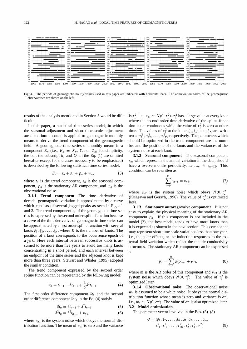
servatories distributed worldwide. The data are collectedthrough the World Data Center system (e.g., see http://swdcdb.kugi.kyoto-u.ac.jp/). The time series atan observatory should be continuous for more than ten years,since a geomagnetic jerk is a sudden change in the trendsof geomagnetic secular variation. A missing period shorterthan about one year is accepted, and it is unnecessary tobe interpolated before the analysis because all componentsexcept for an observational noise component in a statisti-cal model can be estimated by the Kalman filter algorithmeven for the missing period (Kitagawa and Gersch, 1996) asmentioned in the next section. The time series of 124 geo-magnetic observatories are selected according to the criteriamentioned above. The distribution of these observatories isshown in Fig. 3. We use the time series from 1957 (IGY)to 1999 but do not before the IGY, for the worldwide cov-erage of the observatories available is not enough. The pe-riod of data available at each observatory is shown in Fig. 4.Obvious artificial spikes and baseline jumps in the data arecorrected manually before the analysis. Unfortunately smallerrors which would affect the result of statistical time se-ries analysis may remain even after this manual correction.However, we can avoid artifacts due to such small errors by acareful check for the results based on the comparison of theresults with those obtained at other observations as shown inSection 4.

A vector of geomagnetic hourly mean value at the i-thobservatory Oi is expressed as Bn,d,h(Oi ) = (Xn,d,h(Oi ),

Yn,d,h(Oi ), Zn,d,h(Oi ))T , where n is the consecutive month

from January 1957, d is the day of the month, and h (h =1, 2, . . . , 24) is the local time. The superscript T denotesthe transpose operation. Hourly means at h = 1, 2, . . . , and24 correspond to the averages in the periods 0000–0100 LT,0100–0200 LT, . . . , and 2300–2400 LT, respectively. The

Fig. 3. The distribution of the 124 geomagnetic observatories whose dataare used in this paper.

monthly means of each local time are computed from thehourly means by

Bn,h(Oi ) = 1

Dn

Dn∑d=1

Bn,d,h(Oi ), (1)

where Dn is the number of days of the month n.

3. Method of Analysis3.1 Statistical time series model

Most of the papers assume that the geomagnetic jerks oc-curred around 1969, 1978, and 1991, and then obtain thejerk amplitudes. Their methods, however, are subjective inthe determination of the occurrence epochs of jerks, and theestimated jerk amplitudes may not be reliable as has beenpointed out by, for example, Alldredge (1984). Stewart andWhaler (1995) and Alexandrescu et al. (1995) developedthe objective methods with the optimal piecewise regressionanalysis and the wavelet analysis, respectively, for deter-mining the occurrence epochs of jerks. The former methodwas applied to geomagnetic annual means, but it is better toadopt monthly means rather than annual means for jerk anal-yses, because the abrupt change occur only in a few years asseen in Figs. 1 and 2, and the temporal resolution of annualmeans may not be sufficient to analyze the jerk. The lat-ter method, on the other hand, was applied to geomagneticmonthly means and succeeded in the objective determina-tion of jerk epochs. Alexandrescu et al. (1995) and Alexan-drescu et al. (1996) proposed a general expression for a jerksignal

j (t) = β H(t − t0)(t − t0)α, (2)

where t0 is the jerk epoch, α is the regularity, β is the am-plitude, and H(t) is the Heaviside function. Alexandrescuet al. (1995) and Alexandrescu et al. (1996) applied thewavelet analysis to geomagnetic data, and evaluated the reg-ularity to be closer 1.5 rather than to 2. This may indicatethat a model with non-integer α value can be applicable tothe trend component, but the second order spline functionis adopted in this paper otherwise physical interpretation of


1960 1970 1980 1990 2000

AAA

AAE

ABG

ABK

AGN

AIA

ALE

AML

AMS

ANN

API

AQU

ARS

ART

ASH

BEL

BFE

BJI

BLC

BNG

BOU

BRW

BSL

CBB

CCS

1960 1970 1980 1990 2000

CLF

CMO

CNB

CWE

CZT

DAL

DIK

DOU

DRV

DVS

ESK

EYR

FCC

FRD

FRN

FUR

GDH

GNA

GUA

GWC

GZH

HAD

HBA

HBK

HER

1960 1970 1980 1990 2000

HIS

HLP

HON

IRT

ISK

KAK

KGD

KIV

KNY

KZN

LER

LNN

LNP

LOV

LQA

LRV

LVV

MAW

MBC

MBO

MEA

MGD

MIR

MMB

MMK

1960 1970 1980 1990 2000

MNK

MOL

MOS

MUT

NEW

NGK

NUR

NVL

NVS

ODE

OTT

PAF

PAG

PBQ

PET

PMG

POD

PPT

RES

RSV

SBA

SIT

SJG

SNA

SOD

1960 1970 1980 1990 2000

SSH

STJ

SVD

SZT

TAN

TEO

TFS

THL

TIK

TKT

TRD

TSU

TUC

UJJ

VAL

VIC

VLA

VOS

VSS

WIT

WNG

YAK

YKC

YSS

Fig. 4. The periods of geomagnetic hourly values used in this paper are indicated with horizontal bars. The abbreviation codes of the geomagneticobservatories are shown on the left.

results of the analysis mentioned in Section 5 would be dif-ficult.

In this paper, a statistical time series model, in whichthe seasonal adjustment and short time scale adjustmentare taken into account, is applied to geomagnetic monthlymeans to derive the trend component of the geomagneticfield. A geomagnetic time series of monthly means in acomponent En (i.e., En = Xn , Yn , or Zn; for simplicity,the bar, the subscript h, and Oi in the Eq. (1) are omittedhereafter except for the cases necessary to be emphasized)is described by the following statistical time series model:

En = tn + sn + pn + wn, (3)

where tn is the trend component, sn is the seasonal com-ponent, pn is the stationary AR component, and wn is theobservational noise.

3.1.1 Trend component The time derivative ofdecadal geomagnetic variation is approximated by a curvewhich consists of several jagged peaks as seen in Figs. 1and 2. The trend component tn of the geomagnetic time se-ries is expressed by the second order spline function becausea curve of the time derivative of geomagnetic time series canbe approximated by a first order spline function with severalknots ξ1, ξ2, . . . , ξK , where K is the number of knots. Theposition of a knot corresponds to the occurrence epoch ofa jerk. Here each interval between successive knots is as-sumed to be more than five years to avoid too many knotsconcentrating in a short period, and each interval betweenan endpoint of the time series and the adjacent knot is keptmore than three years. Stewart and Whaler (1995) adoptedthe similar condition.

The trend component expressed by the second orderspline function can be represented by the following model:

tn = tn−1 + δtn−1 + 1

2δ2tn−1. (4)

The first order difference component δtn and the secondorder difference component δ2tn in the Eq. (4) satisfy

δtn = δtn−1 + δ2tn−1 (5)

δ2tn = δ2tn−1 + vn1, (6)

where vn1 is the system noise which obeys the normal dis-tribution function. The mean of vn1 is zero and the variance

is τ 21 , i.e., vn1 ∼ N (0, τ 2

1 ). τ 21 has a large value at every knot

where the second order time derivative of the spline func-tion is not continuous while the value of τ 2

1 is zero at othertime. The values of τ 2

1 at the knots ξ1, ξ2, . . . , ξK are writ-ten as τ 2

11, τ212, . . . , τ 2

1K , respectively. The parameters whichshould be optimized in the trend component are the num-ber and the positions of the knots and the variances of thesystem noise at each knot.

3.1.2 Seasonal component The seasonal componentsn , which represents the annual variation in the data, shouldhave a twelve months periodicity, i.e., sn ≈ sn−12. Thiscondition can be rewritten as

11∑i=0

sn−i = vn2, (7)

where vn2 is the system noise which obeys N (0, τ 22 )

(Kitagawa and Gersch, 1996). The value of τ 22 is optimized

later.3.1.3 Stationary autoregressive component It is not

easy to explain the physical meaning of the stationary ARcomponent pn . If this component is not included in themodel (3), the best model tends to have more knots thanit is expected as shown in the next section. This componentmay represent short time scale variations less than one year,i.e., the solar effects, or the induction responses to the ex-ternal field variation which reflect the mantle conductivitystructures. The stationary AR component can be expressedas

pn =m∑

i=1

ai pn−i + vn3, (8)

where m is the AR order of this component and vn3 is thesystem noise which obeys N (0, τ 2

3 ). The value of τ 23 is

optimized later.3.1.4 Observational noise The observational noise

wn is assumed to be a white noise. It obeys the normal dis-tribution function whose mean is zero and variance is σ 2,i.e., wn ∼ N (0, σ 2). The value of σ 2 is also optimized later.3.2 Model optimization

The parameter vector involved in the Eqs. (3)–(8)

θ = (ξ1, ξ2, . . . , ξK , a1, a2, . . . , am,

τ 211, τ

212, . . . , τ 2

1K , τ 22 , τ 2

3 , σ 2) (9)


is estimated simultaneously by the maximum likelihoodmethod. The optimum parameter vector θ (The hat means“optimum” ) that makes the log-likelihood function �(θ)

maximum should be estimated by a numerical method be-cause it is hard to obtain it analytically. The value of thelog-likelihood �(θ) for a given parameter vector θ can becalculated simply by the Kalman filter algorithm through thestate space model (Anderson and Moore, 1979). The statespace model can be constructed as

xn = Fxn−1 + Gvn (10)

En = Hxn + wn (11)

from the Eqs. (3)–(8) by defining the state space vector xn

and the system noise vector vn as

xn = (tn δtn δ2tnsn sn−1 · · · sn−10

pn pn−1 · · · pn−m+1)T (12)

vn = (vn1 vn2 vn3)T , (13)

and the matrices F , G, and H as

F =

1 1 1/2

0 1 1

0 0 1

−1 · · · −1 −1

1. . .

1

a1 · · · am−1 am

1. . .

1

(14)

G =

0

0

1

1

0...

0

1

0...

0

(15)

H = (1 0 0︸︷︷︸3

| 1 0 · · · 0︸︷︷︸11

| 1 0 · · · 0︸︷︷︸m

). (16)

First an appropriate initial parameter vector θ0 is givenand the log-likelihood function �(θ0) is calculated by theKalman filter. Then the parameter vector is updated bythe quasi-Newton method (Press et al., 1986) to make thelog-likelihood larger. This procedure is iterated until theparameter vector θ makes the log-likelihood maximum. TheAIC

AIC = −2�(θ) + 2 dim θ

={

−2�(θ) + 2(2K + 2) (m = 0)

−2�(θ) + 2(2K + m + 3) (m = 0)(17)

is employed to select the best model among the models withdifferent number of the parameters. The model which makesthe AIC minimum is assumed to be the best model for thetime series. See Higuchi and Ohtani (2000) for an applica-tion of the AIC to determination of the number and positionsof the knots. The final estimate of the state vector variable isobtained by the fixed interval smoother algorithm (Kitagawaand Gersch, 1996). The optimum positions of the knots aretreated as candidates for jerk occurrence. It should be notedthat, because our procedure detects any jerk regardless ofits origin (internal or external one), the knot positions deter-mined must undergo further analyses, i.e., an examinationof spatial and local time dependency of occurrence rate andjerk amplitude as explained in Sections 4 and 5. As a result,the jerk of external origin and one due to small artificial er-rors can be excluded. The jerk amplitude δ3 En at a knot ξi

is defined as:

δ3 Eξi = δ2tξi − δ2tξi −1. (18)

The unit of this jerk amplitude is not nT/year3 but nT/year2

because it is defined as a simple difference between suc-cessive second order difference components. The similardefinition of the jerk amplitude (Eq. (18)) is given by theprevious papers (e.g., De Michelis et al., 1998).

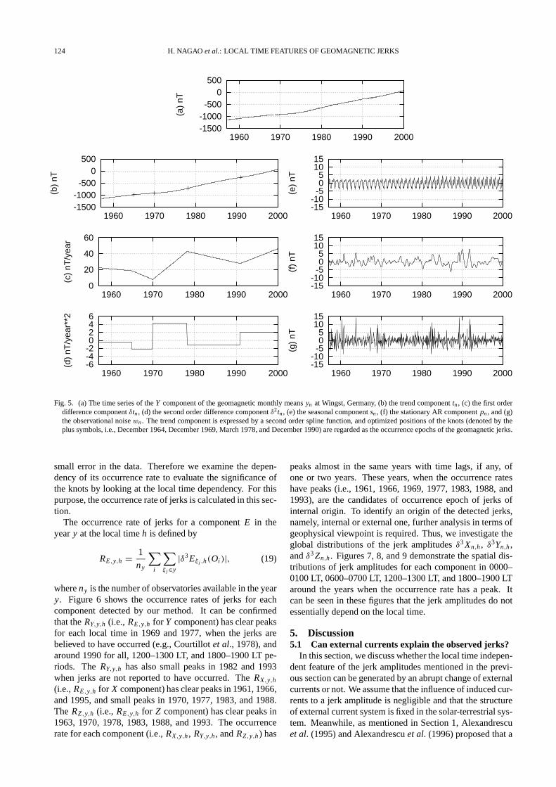
4. ResultsAn example of the decomposition of geomagnetic time

series by the method mentioned in the previous section isshown in Fig. 5. The data used in Fig. 5 are the monthlymeans of the Y component at Wingst (53.75◦N, 9.07◦E),Germany, obtained from 0000–0100 LT. Although there ex-ist missing period for July and August 1968, they can be in-terpolated automatically by the Kalman filter (Anderson andMoore, 1979). The number of the knots for the best modelis K = 4 and they locate at ξ1 = December 1964, ξ2 =December 1969, ξ3 = March 1978, and ξ4 = December1990, when the jerks are believed to have occurred exceptfor 1964. Other parameter values for the best model arem = 2, a1 = 1.32 nT, a2 = −0.487 nT, τ 2

11 = 1.59 × 10−5

nT2, τ 212 = 9.48 × 10−5 nT2, τ 2

13 = 8.18 × 10−5 nT2, τ 214 =

1.30 × 10−3 nT2, τ 22 = 6.84 × 10−3 nT2, τ 2

3 = 1.00 × 10−2

nT2, and σ 2 = 10.3 nT2. The log-likelihood is −1526.29and the AIC is 3078.52. The seasonal component has theamplitude of ∼4 nT. The number of the knots becomes5 and the AIC increases to 3126.22 if the stationary ARcomponent pn is not included in the model (3), which in-dicates an advantage of including the stationary AR compo-nent. The same tendency is seen in most of the cases. Theamplitudes of sn , pn , and wn tend to be amplified and theAR order m tends to increase when the data at high or lowlatitude observatories are used or when the daytime data areused.

As mentioned in Subsection 3.2, not all of the detectedjerks are of internal origin. For example, the optimal knotξ1 detected at Wingst may reflect a local phenomenon or a


-1500-1000-500

0500

1960 1970 1980 1990 2000

(a)

nT

-1500-1000-500

0500

1960 1970 1980 1990 2000

(b)

nT

0

20

40

60

1960 1970 1980 1990 2000

(c)

nT/y

ear

-6-4-20246

1960 1970 1980 1990 2000

(d)

nT/y

ear*

*2

-15-10-505

1015

1960 1970 1980 1990 2000

(e)

nT-15-10-505

1015

1960 1970 1980 1990 2000(f

) nT

-15-10-505

1015

1960 1970 1980 1990 2000

(g)

nT

Fig. 5. (a) The time series of the Y component of the geomagnetic monthly means yn at Wingst, Germany, (b) the trend component tn , (c) the first orderdifference component δtn , (d) the second order difference component δ2tn , (e) the seasonal component sn , (f) the stationary AR component pn , and (g)the observational noise wn . The trend component is expressed by a second order spline function, and optimized positions of the knots (denoted by theplus symbols, i.e., December 1964, December 1969, March 1978, and December 1990) are regarded as the occurrence epochs of the geomagnetic jerks.

small error in the data. Therefore we examine the depen-dency of its occurrence rate to evaluate the significance ofthe knots by looking at the local time dependency. For thispurpose, the occurrence rate of jerks is calculated in this sec-tion.

The occurrence rate of jerks for a component E in theyear y at the local time h is defined by

RE,y,h = 1

ny

∑i

∑ξ j ∈y

|δ3 Eξ j ,h(Oi )|, (19)

where ny is the number of observatories available in the yeary. Figure 6 shows the occurrence rates of jerks for eachcomponent detected by our method. It can be confirmedthat the RY,y,h (i.e., RE,y,h for Y component) has clear peaksfor each local time in 1969 and 1977, when the jerks arebelieved to have occurred (e.g., Courtillot et al., 1978), andaround 1990 for all, 1200–1300 LT, and 1800–1900 LT pe-riods. The RY,y,h has also small peaks in 1982 and 1993when jerks are not reported to have occurred. The RX,y,h

(i.e., RE,y,h for X component) has clear peaks in 1961, 1966,and 1995, and small peaks in 1970, 1977, 1983, and 1988.The RZ ,y,h (i.e., RE,y,h for Z component) has clear peaks in1963, 1970, 1978, 1983, 1988, and 1993. The occurrencerate for each component (i.e., RX,y,h , RY,y,h , and RZ ,y,h) has

peaks almost in the same years with time lags, if any, ofone or two years. These years, when the occurrence rateshave peaks (i.e., 1961, 1966, 1969, 1977, 1983, 1988, and1993), are the candidates of occurrence epoch of jerks ofinternal origin. To identify an origin of the detected jerks,namely, internal or external one, further analysis in terms ofgeophysical viewpoint is required. Thus, we investigate theglobal distributions of the jerk amplitudes δ3 Xn,h , δ3Yn,h ,and δ3 Zn,h . Figures 7, 8, and 9 demonstrate the spatial dis-tributions of jerk amplitudes for each component in 0000–0100 LT, 0600–0700 LT, 1200–1300 LT, and 1800–1900 LTaround the years when the occurrence rate has a peak. Itcan be seen in these figures that the jerk amplitudes do notessentially depend on the local time.

5. Discussion5.1 Can external currents explain the observed jerks?

In this section, we discuss whether the local time indepen-dent feature of the jerk amplitudes mentioned in the previ-ous section can be generated by an abrupt change of externalcurrents or not. We assume that the influence of induced cur-rents to a jerk amplitude is negligible and that the structureof external current system is fixed in the solar-terrestrial sys-tem. Meanwhile, as mentioned in Section 1, Alexandrescuet al. (1995) and Alexandrescu et al. (1996) proposed that a


X Y Z

All

nT/y

ear2

0

0.5

1

1.5

2

1960 1970 1980 1990 20000

0.5

1

1.5

2

1960 1970 1980 1990 20000

0.5

1

1.5

2

1960 1970 1980 1990 2000

0000

-010

0LT

nT/y

ear2

0

0.5

1

1.5

2

1960 1970 1980 1990 20000

0.5

1

1.5

2

1960 1970 1980 1990 20000

0.5

1

1.5

2

1960 1970 1980 1990 2000

0600

-070

0LT

nT/y

ear2

0

0.5

1

1.5

2

1960 1970 1980 1990 20000

0.5

1

1.5

2

1960 1970 1980 1990 20000

0.5

1

1.5

2

1960 1970 1980 1990 2000

1200

-130

0LT

nT/y

ear2

0

0.5

1

1.5

2

1960 1970 1980 1990 20000

0.5

1

1.5

2

1960 1970 1980 1990 20000

0.5

1

1.5

2

1960 1970 1980 1990 2000

1800

-190

0LT

nT/y

ear2

0

0.5

1

1.5

2

1960 1970 1980 1990 20000

0.5

1

1.5

2

1960 1970 1980 1990 20000

0.5

1

1.5

2

1960 1970 1980 1990 2000

Fig. 6. The occurrence rate of geomagnetic jerks for each component obtained from all of the local time (the top three panels) and at each local time. Theoccurrence rate is defined by Eq. (19).

jerk is not just the change in the secular variation trend butalso the behavior of the field over the next decade. Howeverwe discuss the results based on classical definition of jerks,i.e., “a jerk is a sudden change in secular variation trends.”

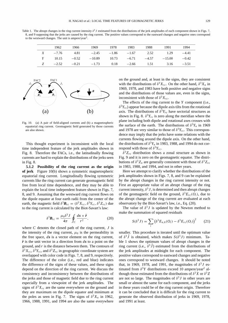
5.1.1 Possibility of field-aligned current as the originof jerk As a simple example, Fig. 10(a) shows a pair ofFACs which produce magnetic disturbance on the ground.An FAC (denoted as FAC1) flows into the dawn side of theionosphere at high latitude region, and another one (denotedas FAC2) flows out from the dusk side of the ionosphere.

The current intensities of FAC1 and FAC2 must be equal(= J ) in order to keep the current continuity. FAC1 gen-erates westward geomagnetic field Y1 at a mid-latitude ob-servatory while FAC2 generates eastward field Y2. Assum-ing that J varies as J = J0eiωt , i.e., Y1 and Y2 vary asY1 = −Y0eiωt and Y2 = Y0eiωt , respectively, we can eas-ily obtain δ3Y1 = −δ3Y2; the signs of the jerk amplitudesare opposite. Generally speaking, a jerk amplitude shoulddepend on the local time not only in its magnitude but alsoin its sign if FACs are the origins of the jerks.


0000-0100LT 0600-0700LT 1200-1300LT 1800-1900LT19

6219

6619

6919

7819

8319

8819

9119

94

Fig. 7. The distributions of the jerk amplitudes for the X component δ3 X in periods 1961–1963, 1965–1967, 1968–1970, 1977–1979, 1982–1984,1987–1989, 1990–1992, and 1993–1995 obtained from the data at 0000–0100 LT, 0600–0700 LT, 1200–1300 LT, and 1800–1900 LT. The blue circlesshow positive values and the red ones show negative values. The magnitude of the jerk amplitudes is represented by the radius of the circles. Thebackground color contour indicates the effects of the westward ring current in the X component estimated by a simple model calculation.


0000-0100LT 0600-0700LT 1200-1300LT 1800-1900LT19

6219

6619

6919

7819

8319

8819

9119

94

Fig. 8. The distributions of the jerk amplitudes for the Y component δ3Y in periods 1961–1963, 1965–1967, 1968–1970, 1977–1979, 1982–1984,1987–1989, 1990–1992, and 1993–1995 obtained from the data at 0000–0100 LT, 0600–0700 LT, 1200–1300 LT, and 1800–1900 LT. The blue circlesshow positive values and the red ones show negative values. The magnitude of the jerk amplitudes is represented by the radius of the circles. Thebackground color contour indicates the effects of the westward ring current in the Y component estimated by a simple model calculation.


0000-0100LT 0600-0700LT 1200-1300LT 1800-1900LT19

6219

6619

6919

7819

8319

8819

9119

94

Fig. 9. The distributions of the jerk amplitudes for the Z component δ3 Z in periods 1961–1963, 1965–1967, 1968–1970, 1977–1979, 1982–1984,1987–1989, 1990–1992, and 1993–1995 obtained from the data at 0000–0100 LT, 0600–0700 LT, 1200–1300 LT, and 1800–1900 LT. The blue circlesshow positive values and the red ones show negative values. The magnitude of the jerk amplitudes is represented by the radius of the circles. Thebackground color contour indicates the effects of the westward ring current in the Z component estimated by a simple model calculation.


Table 1. The abrupt changes in the ring current intensity δ3 J estimated from the distributions of the jerk amplitudes of each component shown in Figs. 7,8, and 9 supposing that the jerks are caused by the ring current. The positive values correspond to the eastward changes and negative ones correspondto the westward changes. The unit is ampere/year2.

1962 1966 1969 1978 1983 1988 1991 1994

X −7.76 4.81 −2.45 −1.86 −1.67 2.52 1.29 −4.41

Y 10.15 −0.52 −10.89 10.73 −6.71 −4.57 −15.00 −0.42

Z −2.52 −0.21 −1.73 0.18 −2.66 1.51 3.16 −3.51

(a) (b)

Fig. 10. (a) A pair of field-aligned currents and (b) a magnetosphericequatorial ring current. Geomagnetic field generated by those currentsare also shown.

This thought experiment is inconsistent with the localtime independent feature of the jerk amplitudes shown inFig. 8. Therefore the FACs, i.e., the latitudinally flowingcurrents are hard to explain the distributions of the jerks seenin Fig. 8.

5.1.2 Possibility of the ring current as the originof jerk Figure 10(b) shows a symmetric magnetosphericequatorial ring current. Longitudinally flowing symmetriccurrents like the ring current can generate geomagnetic fieldfree from local time dependence, and they may be able toexplain the local time independent feature shown in Figs. 7,8, and 9. Assuming that the westward ring current flows onthe dipole equator at four earth radii from the center of theearth, the magnetic field δ3Brc = (δ3 Xrc, δ

3Yrc, δ3 Zrc) due

to the ring current is calculated by the Biot-Savart’s law:

δ3Brc = µ0δ3 J

4π

∮C

ds × rr2

, (20)

where C denotes the closed path of the ring current, J isthe intensity of the ring current, µ0 is the permeability inthe free space, ds is a vector element on the ring current,r is the unit vector in a direction from ds to a point on theground, and r is the distance between them. The contours ofδ3 Xrc, δ3Yrc, and δ3 Zrc in geographic coordinate system areoverlapped with color code in Figs. 7, 8, and 9, respectively.The difference of the color (i.e., red and blue) indicatesthe difference of the signs of these values, and these signsdepend on the direction of the ring current. We discuss theconsistency and inconsistency between the distributions ofthe jerks and those of magnetic field due to the ring currentespecially from a viewpoint of the jerk amplitudes. Thesigns of δ3 Xrc are the same everywhere on the ground andthey are maximum on the dipole equator and minimum atthe poles as seen in Fig. 7. The signs of δ3 Xn in 1962,1966, 1988, 1991, and 1994 are also the same everywhere

on the ground and, at least in the signs, they are consistentwith the distributions of δ3 Xrc. On the other hand, δ3 Xn in1969, 1978, and 1983 have both positive and negative signsand the distributions of those values are, even in the signs,inconsistent with those of δ3 Xrc.

The effects of the ring current to the Y component (i.e.,δ3Yrc) appear because the dipole axis tilts from the rotationalaxis. The distributions of δ3Yrc have sectorial structures asshown in Fig. 8. δ3Yrc is zero along the meridian where theplane including both dipole and rotational axes crosses withthe surface of the earth. The distributions of δ3Yn in 1969and 1978 are very similar to those of δ3Yrc. This correspon-dence may imply that the jerks have some relations with thecurrents flowing around the dipole axis. On the other hand,the distributions of δ3Yn in 1983, 1988, and 1994 do not cor-respond with those of δ3Yrc.

δ3 Zrc distribution shows a zonal structure as shown inFig. 9 and it is zero on the geomagnetic equator. The distri-butions of δ3 Zn are generally consistent with those of δ3 Zrc

in 1983, 1988, and 1994, and not in other years.Here we attempt to clarify whether the distributions of the

jerk amplitudes shown in Figs. 7, 8, and 9 can be explainedby the abrupt changes in the ring current intensity or not.First an appropriate value of an abrupt change of the ringcurrent intensity, δ3 J , is determined and then abrupt changesof the geomagnetic field on the ground, δ3 Erc(Oi ), due tothe abrupt change of the ring current are evaluated at eachobservatory by the Biot-Savart’s law, i.e., Eq. (20).

The value of δ3 J is updated by the Newton method tomake the summation of squared residuals

S(δ3 J ) =∑

i

(δ3 En,h(Oi ) − δ3 Erc(Oi )

)2(21)

smaller. This procedure is iterated until the optimum valueof δ3 J is obtained, which makes S(δ3 J ) minimum. Ta-ble 1 shows the optimum values of abrupt changes in thering current (i.e., δ3 J ) estimated from the distributions ofthe jerk amplitudes at midnight for each component. Thepositive values correspond to eastward changes and negativeones correspond to westward changes. It should be notedthat, in 1969, 1978, and 1991, the magnitudes of δ3 J es-timated from δ3Y distributions exceed 10 ampere/year2 al-though those estimated from the distributions of δ3 X or δ3 Zare not so large. The magnitudes of δ3 J in other years aresmall or almost the same for each component, and the jerksin these years could be of the ring current origin. Thereforeit can be concluded that it is difficult for the ring current togenerate the observed distribution of jerks in 1969, 1978,and 1991 at least.

130 H. NAGAO et al.: LOCAL TIME FEATURES OF GEOMAGNETIC JERKS19

6919

7819

91

Fig. 11. The global distribution of the occurrence epochs of detected jerksat each observatory for the 1969 (the top panel), the 1978 (the middlepanel), and 1991 (the bottom panel) events. The monthly means at0000–0100LT are used. The blue circles denote early arrivals of jerksbefore 1970, 1979, and 1992, respectively, and the red ones denote latearrivals of jerks after 1971, 1980, and 1993, respectively.

From the discussion mentioned above, it is difficult forglobal external currents like the FACs or the ring current toexplain the observed jerks in 1969, 1978, and 1991, and it ismore natural to consider that these jerks are of internal ori-gin. More detailed analyses of the jerks with more extensivedata set are required to investigate the physical mechanismswhich can generate the observed jerks.5.2 Time lags in the occurrence epochs of 1991 jerk

It has been reported that the occurrence epochs of jerksare not simultaneous to the global extent but have time lagswith a few years. Alexandrescu et al. (1996) showed that the

jerks occurred in the southern hemisphere a few years afterthe occurrences of the 1969 and 1978 jerks in the northernhemisphere. De Michelis et al. (1998) showed that the jerkoccurred in North and South America a few years beforethe occurrence of the 1991 jerk in other regions. The resultof our analysis on this topic obtained from 0000–0100 LTdata shown in Fig. 11 clearly demonstrates that the jerksoccurred in the southern hemisphere except for Antarcticaobservatories a few years after the occurrences of the 1969and 1978 jerks in the northern hemisphere. This result is ingood agreement with Alexandrescu et al. (1996). We foundthat the jerk occurred in the southern hemisphere a few yearsafter the occurrence of the 1991 jerk in Europe, which issimilar to the time delay for the 1969 and 1978 jerks. Thesetime lags in the occurrence epochs of the 1969, 1978, and1991 jerks could be due to the mantle conductivity filteringeffect (e.g., Backus, 1983; Alexandrescu et al., 1996).

6. ConclusionsWe analyzed the time series of geomagnetic monthly

means of the X , Y , and Z components at each local timeto clarify the origins and distributions of geomagnetic jerks.Each geomagnetic time series is decomposed into the trend,the seasonal, the stationary AR, and the observational noisecomponents by applying a statistical time series model. Thetrend component is expressed by a second order spline func-tion because a jerk is an impulse in the third order timederivative of the geomagnetic time series. The model pa-rameters including the positions of the knots of the splinefunction are estimated by the maximum likelihood methodand the number of the knots and the AR order are selectedbased on the AIC. Distributions of jerk amplitudes are ob-tained by regarding the optimized positions of the knots asthe occurrence epochs of the jerks.

We obtained the following results: The distributions ofthe geomagnetic jerks are essentially independent of localtime. Longitudinally flowing external currents like the ringcurrent may be able to generate such distributions of thejerks while latitudinally flowing external currents like theFACs cannot generate such distributions. If we assume thatthe ring current is the source of the geomagnetic jerks, themagnitude of the abrupt changes in the ring current intensi-ties estimated from the jerk amplitudes of the Y componentexceed, by an order of magnitude, those obtained from thejerk amplitudes of the X or the Z components in 1969, 1978,and 1991. The distributions of the jerks in 1969, 1978, and1991 are difficult to be explained by the external currentssuch as the FACs or the ring currents. Therefore it is moreplausible that the geomagnetic jerks in 1969, 1978, and 1991are not of external origin but internal one if we ignore theeffects of induced currents due to inhomogeneous conduc-tivity of the crust or the mantle, although the physical mech-anism which generates the observed jerks is still unknown.

We also obtain a new result as to the time lags betweenthe occurrence epoch of the 1991 jerk in the northern hemi-sphere and that in the southern hemisphere. While it is con-firmed that the occurrences of the jerks in the southern hemi-sphere a few years after those of the 1969 and 1978 jerks inthe northern hemisphere as pointed out by Alexandrescu etal. (1996) and De Michelis et al. (1998), it is also found that


the occurrence of the jerk in the southern hemisphere is afew years after that of the 1991 jerk in Europe. Taking thesetime lags in occurrence epochs of the jerks into account, the1969, 1978, and 1991 jerks are confirmed to be global phe-nomena as suggested by previous papers.

Acknowledgments. We are grateful to staff of Data Analysis Cen-ter for Geomagnetism and Space Magnetism, Graduate School ofScience, Kyoto University for supplying us the high quality geo-magnetic data. We also thank to Y. Yokoyama, S. Ohtani, A. Saitoand G. Ueno for the personal discussions and their valuable advice.Miora Mandea and another anonymous referee are also appreci-ated for reviewing our paper and giving us valuable comments.This research was supported by the Ministry of Education, Science,Sports and Culture (MESSC) of Japan, Grant-in-Aid for ScientificResearch on Priority Area “Discovery Science,” 10143106, 1998–2001. Work at the Institute of Statistical Mathematics was in partcarried out under the ISM Cooperative Research Program (H12-ISM.CRP-2026). The computation in this work has been done us-ing SGI2800 of the Institute of Statistical Mathematics.

ReferencesAchache, J., V. Courtillot, J. Ducruix, and J.-L. Le Mouel, The late 1960’s

secular variation impulse: further constraints on deep mantle conductiv-ity, Phys. Earth Planet. Int., 23, 72–75, 1980.

Alexandrescu, M., D. Gibert, G. Hulot, J.-L. Le Mouel, and G. Saracco,Detection of geomagnetic jerks using wavelet analysis, J. Geophys. Res.,100, 12557–12572, 1995.

Alexandrescu, M., D. Gibert, G. Hulot, J.-L. Le Mouel, and G. Saracco,Worldwide wavelet analysis of geomagnetic jerks, J. Geophys. Res., 101,21975–21994, 1996.

Alldredge, L. R., A discussion of impulses and jerks in the geomagneticfield, J. Geophys. Res., 89, 4403–4412, 1984.

Alldredge, L. R., More on the alleged 1970 geomagnetic jerk, Phys. EarthPlanet. Int., 39, 255–264, 1985.

Anderson, B. D. O. and J. B. Moore, Optimal Filtering, Prentice-Hall,1979.

Backus, G. E., Application of mantle filter theory to the magnetic jerk of1969, Geophys. J. R. astr. Soc., 74, 713–746, 1983.

Cafarella, L. and A. Meloni, Evidence for a geomagnetic jerk in 1990across Europe, Annali di Geofisica, XXXVIII, 451–455, 1995.

Courtillot, V., J. Ducruix, and J.-L. Le Mouel, Sur une acceleration recentede la variation seculaire du champ magnetique terrestre, C. R. Acad.Serie D, 1095–1098, 1978.

Davis, R. G. and K. A. Whaler, The 1969 geomagnetic impulse and spin-upof the Earth’s liquid core, Phys. Earth Planet. Int., 103, 181–194, 1997.

De Michelis, P., L. Cafarella, and A. Meloni, Worldwide character of the1991 geomagnetic jerk, Geophys. Res. Lett., 25, 377–380, 1998.

Ducruix, J., V. Courtillot, and J.-L. Le Mouel, The late 1960s secularvariation impulse, the eleven year magnetic variation and the electricalconductivity of the deep mantle, Geophys. J. R. astr. Soc., 61, 73–94,1980.

Gavoret, J., D. Gibert, M. Menvielle, and J.-L. Le Mouel, Long-termvariations of the external and internal components of the earth’s magneticfield, J. Geophys. Res., 91, 4787–4796, 1986.

Golovkov, V. P., T. I. Zvereva, and A. O. Simonyan, Common featuresand differences between “ jerks” of 1947, 1958 and 1969, Geophys.Astrophys. Fluid Dyn., 49, 81–96, 1989.

Gubbins, D. and L. Tomlinson, Secular variation from monthly means fromApia and Amberley magnetic observatories, Geophys. J. R. astr. Soc., 86,603–616, 1986.

Higuchi, T. and S. Ohtani, Automatic identification of large-scale field-aligned current structures, J. Geophys. Res., 105, 25305–25315, 2000.

Kerridge, D. J. and D. R. Barraclough, Evidence for geomagnetic jerksfrom 1931 to 1971, Phys. Earth Planet. Int., 39, 228–236, 1985.

Kitagawa, G. and W. Gersch, Smoothness priors analysis of time series,Lecture Notes in Statistics, 116, Springer-Verlag, New York, 1996.

Le Huy, M., M. Alexandrescu, G. Hulot, and J.-L. Le Mouel, On thecharacteristics of successive geomagnetic jerks, Earth Planets Space, 50,723–732, 1998.

Le Huy, M., M. Mandea, J.-L. Le Mouel, and A. Pais, Time evolution ofthe field flow at the top of the core. Geomagnetic jerks, Earth PlanetsSpace, 52, 163–173, 2000.

Le Mouel, J.-L. and V. Courtillot, Core motions, electromagnetic core-mantle coupling and variations in the earth’s rotation: new constraintsfrom geomagnetic secular variation impulses, Phys. Earth Planet. Int.,24, 236–241, 1981.

Le Mouel, J.-L., J. Ducruix, and C. H. Duyen, The worldwide characterof the 1969–1970 impulse of the secular acceleration rate, Phys. EarthPlanet. Int., 28, 337–350, 1982.

Macmillan, S., A geomagnetic jerk for the early 1990’s, Earth Planet. Sci.Lett., 137, 189–192, 1996.

Malin, S. R. C. and B. M. Hodder, Was the 1970 geomagnetic jerk ofinternal or external origin?, Nature, 296, 726–728, 1982.

Mandea Alexandrescu, M., D. Gibert, J.-L. Le Mouel, G. Hulot, and G.Saracco, An estimate of average lower mantle conductivity by waveletanalysis of geomagnetic jerks, J. Geophys. Res., 104, 17735–17745,1999.

Mandea, M., E. Bellanger, and J.-L. Le Mouel, A geomagnetic jerk for theend of the 20th century?, Earth Planet. Sci. Lett., 183, 369–373, 2000.

McLeod, M. G., On the geomagnetic jerk of 1969, J. Geophys. Res., 90,4597–4610, 1985.

McLeod, M. G., Signals and noise in magnetic observatory annual means:mantle conductivity and jerks, J. Geophys. Res., 97, 17261–17290, 1992.

Nevanlinna, H. and C. Sucksdorff, Impulse in global geomagnetic “secularvariation” , 1977–1979, J. Geophys., 50, 68–69, 1981.

Press, W. H., B. P. Flannery, S. A. Teukolsky, and W. T. Vetterling, Numer-ical Recipes: The Art of Scientific Computing, Cambridge UniversityPress, 1986.

Stewart, D. N. and K. A. Whaler, Optimal piecewise regression analysisand its application to geomagnetic time series, Geophys. J. Int., 121,710–724, 1995.

Thompson, D. and J. C. Cain, The geomagnetic jerk of 1969 and theDGRFs, Phys. Earth Planet. Int., 48, 386–388, 1987.

Whaler, K. A., A new method for analysing geomagnetic impulses, Phys.Earth Planet. Int., 48, 221–240, 1987.

H. Nagao (e-mail: [email protected]), T. Iyemori (e-mail:[email protected]), T. Higuchi (e-mail: [email protected]), S.Nakano (e-mail: [email protected]), and T. Araki (e-mail: [email protected])

Documents

Local time features of geomagnetic jerks - TERRAPUB · Earth Planets Space, 54, 119–131, 2002 Local time features of geomagnetic jerks Hiromichi Nagao1, Toshihiko Iyemori2, Tomoyuki