Local-Prediction-Based Difference Expansion Reversible Watermarking

IEEE TRANSACTIONS ON IMAGE PROCESSING, VOL. 23, NO. 4, APRIL 2014 1779

Local-Prediction-Based Difference ExpansionReversible Watermarking

Ioan-Catalin Dragoi, Member, IEEE, and Dinu Coltuc, Senior Member, IEEE

Abstract— This paper investigates the use of local predictionin difference expansion reversible watermarking. For each pixel,a least square predictor is computed on a square block centeredon the pixel and the corresponding prediction error is expanded.The same predictor is recovered at detection without any addi-tional information. The proposed local prediction is general and itapplies regardless of the predictor order or the prediction context.For the particular cases of least square predictors with the samecontext as the median edge detector, gradient-adjusted predictoror the simple rhombus neighborhood, the local prediction-basedreversible watermarking clearly outperforms the state-of-the-artschemes based on the classical counterparts. Experimental resultsare provided.

Index Terms— Reversible watermarking, difference expansion,adaptive prediction, least square predictors.

I. INTRODUCTION

WHILE classical watermarking introduces permanentdistortions, reversible watermarking not only extracts

the embedded data, but also recovers the original hostsignal/image without any distortion. So far, three majorapproaches have already been developed for image reversiblewatermarking. They are reversible watermarking based onlossless compression, on histogram shifting and on differenceexpansion.

The lossless compression based approach substitutes a partof the host with the compressed code of the substituted partand the watermark [1], [2], etc. In order to avoid artifacts, thesubstitution should be applied on the least significant bits areawhere the compression ratio is poor. This limits the efficiencyof the lossless compression reversible watermarking approach.

A more efficient solution is the histogram shifting approach.The histogram of a pixel based image feature (graylevel[3], pixel difference [4], prediction error [5], interpolationerror [6]) is considered. A histogram bin is selected and thespace for data embedding is created into an adjacent bin (eitherthe bin located at the left or at the right). For instance, letp be the value of the selected bin and let p + 1 (the bin to itsright) be considered for data embedding. The features greater

Manuscript received April 18, 2013; revised October 6, 2013 andDecember 9, 2013; accepted February 12, 2014. Date of publicationFebruary 20, 2014; date of current version March 6, 2014. This work wassupported by UEFISCDI Romania under Grant PN-IIPT-PCCA-2011-3.2-1162. The associate editor coordinating the review of this manuscript andapproving it for publication was Prof. Stefano Tubaro.

The authors are with the Department of Electrical and Electronics Engi-neering, Valahia University Targoviste, Targoviste 130082, Romania (e-mail:[email protected]; [email protected]).

Color versions of one or more of the figures in this paper are availableonline at http://ieeexplore.ieee.org.

Digital Object Identifier 10.1109/TIP.2014.2307482

than p are shifted with one position (by modifying with onegraylevel the value of the corresponding pixels). Furthermore,the embedding is performed into the pixels with the featurevalue equal to p. When a zero is embedded the pixel is leftunchanged, otherwise it is modified with one graylevel inorder to change the feature from p to p + 1. The procedureis similar if p − 1 is considered for embedding, except thatthe shifting proceeds to the left. In a single embedding level,the approach provides an embedding capacity of the sameorder as the size of the selected bin. For this reason, thesimple graylevel histogram used in the original approach of[3] was replaced by Laplacian distributed histograms, with aprominent maximum bin, like the prediction error histogramand so on. The original approach considered the embeddinginto the maximum of the histogram in order to maximize theembedding bit-rate. Several other strategies have also beeninvestigated. For instance, the simultaneous embedding intothe maximum and the second in rank doubles the embeddingbit-rate provided in a single embedding level [7].

For embedding less than the size of the two largest his-togram bins, a very efficient histogram shifting was pro-posed [8]. The embedding is performed into the smallest twobins, one from the left and the other for the right, that providethe needed capacity. Since only the tails of the histogrammust be shifted, the distortion is minimized. As the requiredembedding capacity increases, more embedding stages areperformed. While in a single embedding stage the histogramshifting approach introduces distortion of at most one graylevelper pixel, this is no longer true for multiple embeddinglevels. In such cases, the most efficient approach is differenceexpansion (DE).

Introduced by Tian, [9], DE expands two times the differ-ence between adjacent pairs of pixels. Then, if no overflow orunderflow appears, one bit of data is added to the expandeddifference. In fact, the expansion is a simple multiplication bytwo. Thus, the least significant bit (LSB) of the difference is setto zero and is substituted by a bit of data. The embedded pixelsare identified by using a location map with one bit for eachpair of pixels. The map is lossless compressed and embeddedinto the image as well. At detection, the embedded bits areimmediately recovered as the LSBs of the pixel differencesand the original pixels are recovered. In a single embeddingstage, the scheme provides a bit-rate of at most 0.5 bpp.

In order to gain in embedding capacity, several improve-ments of the original DE scheme have been proposed. Wemention the increase of the theoretical embedding bit-rate from0.5 bpp to n−1

n bpp obtained by simultaneously transforming

1057-7149 © 2014 IEEE. Personal use is permitted, but republication/redistribution requires IEEE permission.See http://www.ieee.org/publications_standards/publications/rights/index.html for more information.

1780 IEEE TRANSACTIONS ON IMAGE PROCESSING, VOL. 23, NO. 4, APRIL 2014

groups of n pixels and embedding n − 1 bits per group [10].The increase is obtained by reducing the size of the locationmap from 1 bit per pair to 1 bit for a group of n pixels.Results are reported for n = 3 or n = 4, where bit-ratescan reach 0.75 bpp. A major advance for the DE algorithmsis the increase of the theoretical embedding bit-rate to 1 bppobtained by embedding into each pixel (see [11]). For medicalimages, a practical solution to increase the embedding bit-rateis the adaptive switching between difference expansion andhistogram shifting in order to embed the large white (or black)regions of such images [12]. Fast DE schemes have also beenproposed [13].

A continuous effort in DE and generally in reversiblewatermarking is devoted to the improvement of the quality ofthe algorithms. The aim is to reduce the embedding distortion.An important advance in this direction is the replacement ofthe location map by a histogram shifting procedure allow-ing the identification of the embedded pixels based on thecorresponding difference [11]. More precisely, the pixels thatcannot be embedded are modified in order to provide, atdetection, a greater difference than the embedded ones. Thepixels that cannot be shifted or embedded are identified byan overflow/underflow map. The overflow/underflow map isconsiderably more efficiently compressed than the originallocation map. On the other hand, the DE with histogramshifting distorts not only the embedded pixels, but also the not-embedded ones. Up to 1 bpp, the DE with histogram shiftingoutperforms the DE with location map. This changes for bit-rates greater than 1 bpp (see [14]) and the implementationswith location map provide better results than the histogramshifting based DE.

A straightforward idea to reduce the embedding distortionconsists of expanding lower differences. The most widely usedapproach is the replacement of the simple pixel difference withthe prediction error (see [11]). Before predictors, let us brieflydiscuss some other ideas. An interesting approach consists ofsorting the pixels based on the smoothness of their context inorder to embed into pixels with low corresponding differences[15]–[17], etc. Another solution considers the embeddingboth by adding and by subtracting the data bit and selectsthe method that minimizes the global distortion [18]. Thedistortion control scheme is also improved in [18]. An adaptivescheme that embeds 2 bits into the pixels of flat regions and1 bit into the pixels of rough regions is proposed in [19]. Thescheme avoids the expansion of pixels where the differences(prediction errors) are susceptible to have large values andat the same time provides high embedding capacity. Theapproach recently proposed in [17] restricts the embedding at3 bits/pair of pixels by eliminating the embedding of “1” intoboth pixels. The loss in embedding bit-rate is minor comparedwith the gain in quality by discarding the case that adds 1 bitof distortion to both pixels. The scheme is efficient mainly forlow embedding bit-rates.

The improvement of the prediction is important for bothhistogram shifting and difference expansion based reversiblewatermarking schemes. The median edge detector predictor(MED) used in [11] and [18], etc., is already a very goodpredictor. We remind you that MED is also used in JPEG-LS

standard [20]. With MED, the prediction context is composedof the right, lower and lower-diagonal neighbors of a pixel.The predictor tends to select the lower vertical neighborin cases where a vertical edge exists right to the currentlocation, the right neighbor in cases of a horizontal edgebelow it, or a linear combination of the context pixels if noedge is detected. The gradient-adjusted predictor (GAP) usedin CALIC (context-based, adaptive, lossless image coding)algorithm [21], outperforms MED. GAP is more complexthan MED. It works on a context of 7 pixels and selects theoutput based not only on the existence of a horizontal/verticaledge, but also on its strength. A simplified version of GAP,SGAP, provides almost similar results, but at a lower cost. Theschemes based on GAP and SGAP outperform the ones basedon MED (see [22]–[24]).

Lower estimation errors than the ones of MED and GAPare provided by the simple average of the four horizontaland vertical neighbors. The problem with the simple averageimmediately appears by considering the usual raster scanordering for watermarking. Each watermarked pixel takes partin the prediction of two other pixels, namely of the righthorizontal and of the lower vertical neighbors. In other words,pixels are predicted by using two original pixel values and twomodified ones. This is because the average of the horizontaland vertical pixels is neither a causal nor an anti-causalpredictor. A better solution is provided by the two stagesembedding of [16]. The image pixels are split in two equalsets, diagonally connected, as the black and white squares ofa chessboard. The watermark is embedded in two stages. Thepixels of a set are marked by using for prediction the pixelsof the other set. The prediction of the first set is done withoriginal pixels, while the one for the second set uses alreadymodified pixels. On the entire image, the overall performanceof the two stages scheme slightly outperforms the direct rasterscan watermarking.

The reversible watermarking of [16] is very efficient.It clearly outperforms the classical DE schemes based onMED or GAP. The overall very good performances of thesimple average on the rhombus context are due to the factthat prediction is performed on an entire neighborhood sur-rounding the pixel and not only on part of it. A contextadaptive version of the rhombus predictor of [16] that providesslightly improved results has been reported in [25]. Thecontext adaptive predictor considers the average of the verticalpixels, the average of the horizontal pixels or the averageof the four horizontal/vertical pixels. In [26], the predictionon the rhombus context is computed by partial differentialequations (PDE). The prediction starts with the average ofthe four horizontal/vertical neighbors. Then, the predictoris updated until stability is reached by considering weightscomputed from the gradients between the four neighbors andthe previous predictor. The PDE predictor may outperformthe simple average on rhombus. In [27], the rhombus contextis extended to the full 3 × 3 window and the central pixelis estimated as 75% of the average of the horizontal/verticalpixels and 25% of the average of the diagonal pixels. A slightlyimproved version of the average on rhombus is obtained bysubtracting a fraction of the prediction error from the upper

DRAGOI AND COLTUC: LOCAL-PREDICTION-BASED DIFFERENCE EXPANSION REVERSIBLE WATERMARKING 1781

pixel and using the raster scan for embedding [28]. The ideais inspired by the context embedding of [24] that spreadsthe expanded prediction error over the prediction context inorder to reduce the overall embedding error. Finally, a moresignificant improvement is reported in [29]. The predictionerror sequence is first computed with the simple average onrhombus and the embedding is done by cleverly substitut-ing blocks of the prediction error sequence with sequencesobtained by decompressing the message bits with codebooksselected in order to minimize the distortion. The informationneeded to recover a block is compressed, concatenated tothe message sequence and embedded in the next block. Theapproach generalizes the prior work of [30].

The prediction can also be improved by using adaptivepredictors. For each image, the coefficients of the predictor arecomputed in order to minimize the prediction error. A popularsolution is the least squares (LS) prediction, namely thesolution minimizes the sum of squares of the prediction error.The LS solution computed for the context of MED usuallyslightly outperforms the results obtained for MED. The use ofLS is somehow natural since the mean square error (PSNR)is used to evaluate the results. Other optimization techniquescan be used as well. For instance, in [31], genetic algorithmsare used for a threshold optimization problem in reversiblewatermarking.

Since image statistics change from one region to another, astraightforward idea is to use multiple local predictors insteadof a single global predictor. Thus, one can split the imageinto blocks and one can compute a distinct LS predictor foreach block. The smaller the blocks, the better the prediction.On the other hand, the use of a predictor for each imageblock increases the size of the additional information. TheLS predictors computed for the entire image or for imageblocks cannot be recovered at detection, since the image ismodified during the marking stage. Thus, the predictors shouldbe embedded into the marked image in order to be available atdetection. This limits the number of predictors in block basedprediction schemes.

This paper investigates the use of local LS prediction inDE reversible watermarking. The basic idea is to compute, foreach pixel, a distinct LS predictor on a block centered on thepixel. The most interesting aspect of our approach is the factthat the same predictor is recovered at detection, avoiding theneed of embedding a large amount of additional information.The proposed local prediction is general and can be appliedregardless of the predictor order or the prediction context.For the particular case of pixel estimation as the average ofits four horizontal and vertical neighbors, the proposed adap-tive reversible watermarking clearly outperforms the schemeof [16], [25], [26], etc. Similarly, the schemes based onlocal prediction on the context of MED, GAP or SGAPsignificantly outperform the classical reversible watermarkingcounterparts.

The outline of the paper is as follows. The differenceexpansion reversible watermarking is briefly reminded inSection II. The local prediction based reversible watermarkingis discussed in Section III. Experimental results and compar-isons with the classical schemes and notably, with the scheme

of [16], are presented in IV. Finally, conclusions are drawn inSection V.

II. DIFFERENCE EXPANSION REVERSIBLE

WATERMARKING

We briefly remind the basic principles of the differenceexpansion with histogram shifting (DE-HS) reversible water-marking for the case of prediction-error expansion (also calledprediction-error expansion). The section introduces the LS pre-diction as well.

A. Basic Reversible Watermarking Scheme

Let x̂i, j be the estimated value of the pixel xi, j .The prediction error is:

ei, j = xi, j − x̂i, j (1)

Let T > 0 be the threshold. The threshold controls thedistortion introduced by the watermark. Thus, if the pre-diction error is less than the threshold and no overflow orunderflow is generated, the pixel is transformed and a bit ofdata, b, is embedded. The transformed pixel is:

x ′i, j = xi, j + ei, j + b (2)

The embedded pixels are also called carrier pixels (see [12]).The pixels that cannot be embedded because |ei, j | ≥ T

(the non-carriers) are shifted in order to provide, at detection,a greater prediction error than the one of the embedded pixels.These pixels are modified as follows:

x ′i, j =

{xi, j + T, if ei, j ≥ T

xi, j − (T − 1), if ei, j ≤ −T .(3)

The underflow/overflow cases are solved either by creating amap of underflow/overflow pixels or by using flag bits [11].

Let us suppose that, at detection, one gets the same predictedvalue for the pixel xi, j . The prediction error at detection is:

e′i, j = x ′

i, j − x̂i, j (4)

The discrimination between embedded and translated pixelsis provided by the prediction error. If −2T ≤ e′

i, j ≤ 2T + 1one has an embedded pixel. For the embedded pixels one hase′

i, j = 2ei, j +b and b follows as the LSB of e′i, j . The original

pixel is immediately recovered as:

x = x ′i, j + x̂i, j − b

2(5)

For the shifted pixels, the original pixel recovery follows byinverting equation (3).

As long as at detection one has the same predicted value, thereversibility of the watermarking scheme is ensured. The samepredicted value is obtained if the pixels within the predictioncontext are recovered before the prediction takes place.

Let us suppose that the watermarking proceeds in a certainscan order. The decoding should proceed in a reverse order.The first pixel restored to its original value is the last embed-ded one. Obviously, for the last embedded pixel, one has thesame prediction context both at detection and at embedding.Once the last embedded pixel has been restored, one recovers


the context for the prediction of its predecessor and so on.Usually, anti-causal predictors are used and the embedding isperformed in raster scan order, row by row, from the upperleft to the lower right pixel. The use of anti-causal predictorswith the normal raster scan has the advantage of using forprediction only the original pixel values.

Before going any further, a comment should be made.In fact, as shown in [24], it is not the predicted value thatshould be exactly recovered at detection, but the expandedprediction error.

The embedding capacity of the basic DE HS scheme is givenby the number of pixels that are embedded with equation (2),namely the pixels having the absolute prediction error lowerthan the threshold. Obviously, the capacity depends on theprediction error, i.e. on the quality of the prediction.

B. Linear Prediction

As said above, adaptive predictors can provide better resultsthan fixed predictors like MED, GAP, the average on the fourhorizontal and vertical neighbors, etc. We shall focus on linearpredictors. By linear prediction, image pixels xi, j are estimatedby a weighted sum over a certain neighborhood of xi, j . Inorder to simplify the notations, we consider an indexing ofthe neighborhood (prediction context), p = 1, . . . , k, namelyx1

i, j , . . . , xki, j , where k is the order of the predictor. Let

v = [v1, . . . , vk]′ be the column vector with the coefficients ofthe predictor. Let xi, j be the row vector obtained by orderingthe context of xi, j according to the indexing. The predictedpixel, x̂i, j = ∑k

p=1 v px pi, j , can be written in closed form as:

x̂i, j = xv (6)

A rather similar form, used mainly in linear regression,includes also a constant term:

x̂i, j = v0 +k∑

p=1

v p x pi, j (7)

When the constant term is used, the vector xi, j is extendedby adding a first element, x0

i, j = 1. We shall consider mainlythis latter form. The predicted value and the prediction errordepend on v. We shall further write x̂i, j (v) and ei, j (v).

A popular solution to the linear regression problem is theleast square (LS) approach. We remind that the LS considersthe weights that minimize the sum of the squares of theprediction error. The LS predictor is the one that provides:

minv

∑i

∑j

ei, j (v)2 (8)

Let y be the column vector obtained by scanning the imagealong the rows and let X be the matrix whose rows are thecorresponding context vectors as defined above. The predictionerror vector is y − Xv. Equation (8) corresponds to the mini-mization of (y−Xv)′(y−Xv), where “′” denotes vector/matrixtransposition. By taking the partial derivatives of the squareerror with respect to the components of v and by setting themequal to zero one gets XX′v = X′y and, finally:

v = (X′X)−1X′y (9)

Fig. 1. Test images: Lena, Mandrill, Jetplane, Barbara, Tiffany and Boat.

TABLE I

THE MEAN SQUARED PREDICTION ERROR FOR RHOMBUS AVERAGE,

GLOBAL PREDICTION AND THE PROPOSED LOCAL PREDICTION

ON SIX STANDARD TEST IMAGES

III. LOCAL PREDICTION REVERSIBLE WATERMARKING

An adaptive global predictor estimates all the pixels of theimage. Since the statistics of the image change from a regionto another, it is very improbable that the predictor will havegood performances everywhere. By dividing the image intoblocks and by computing a distinct predictor for each block,one expects that the predictor will provide better results. Theproblem is to select the size of the blocks or, equivalently, thenumber of blocks. The larger the number of blocks, the betterthe prediction. The limit is the case when one computes onedistinct predictor for each pixel.

In order to illustrate the reduction of the prediction errorprovided by using a distinct predictor for each pixel, a simpleexample is presented. Let us consider the case of the rhombuscontext and let us evaluate the mean squared prediction errorfor local LS prediction computed on a B × B sliding window,with B = {8, 12, 16}. The results for six standard 512 × 512test images, Lena, Mandrill, Jetplane, Barbara, Tiffany andBoat (see Fig. 1) are presented in Table I. From Table Iit clearly appears that, for all three values of B , the localpredictors outperform both the average on the rhombus andthe global predictor. The improvement depends on the imagecontent, namely it is more significant for images with a highcontent of texture or fine details than for the ones with largeuniform areas. Two examples of prediction error histogramsare presented in Fig. 2, one for a predominantly uniform image(Lena) and the other for an image with large textured areas(Barbara).


Fig. 2. The prediction error histograms for the rhombus average, globalprediction and local prediction on two test images.

Fig. 3. Blocks for local predictor computation.

As briefly discussed in Section II-A, the predicted pixelis either embedded or shifted by the reversible watermarkingscheme. Since pixels are modified, the predictor computed onan original block at the embedding stage cannot be recoveredfrom an already embedded block. The solution for such a blockbased scheme is to embed the coefficients of the predictor intothe image as additional information in order to be availableat detection. This strategy limits the number of blocks, sincethe gain obtained by improving the prediction is lost by theincrease of the additional information size.

A. Local Prediction

Next, we investigate the computation of a distinct predictorfor each pixel. Obviously, the embedding of the predictorscoefficients into the image is out of the question. Therefore,instead of computing the predictors on original image blocks,we investigate the computation on blocks containing bothoriginal and modified pixels.

Let the pixels be embedded in a raster-scan order, pixel bypixel and row by row, from the upper left corner to the lowerright one. Obviously, the decoding proceeds in reverse order,from bottom to top, starting with the last embedded pixel.Let us consider the decoding and let xi, j be the currentpixel. Let us take a block of pixels centered on xi, j . If onecompares the block taken at detection, before the decodingof xi, j , with the same block, but taken at embedding, beforethe embedding of xi, j , it immediately appears that only xi, j

is different (Fig. 3). Obviously, since the decoding starts with

the last embedded pixel, all the pixels that follow the currentpixel in the raster-scan order have already been decoded.

The observation that, except the central pixel, the blockscentered on a pixel at embedding are exactly recovered atdetection, suggested to us the computation of the predictor foreach pixel on a B × B block centered on it and the recovery ofthe same predictor at detection. Thus, instead of consideringas in Section II-B, the matrix X and the vector y for theentire image, one should consider a matrix Xi,j and a vectoryi,j by taking only the pixels having the prediction contextincluded into the B × B block centered on the pixel xi, j . Thenthe current predictor vi,j is computed (for instance, by usingequation (9)) and so on.

Obviously, the current pixel cannot be considered in thecomputation of the current predictor. Meanwhile, the currentpixel appears in the prediction context of other pixels of theblock. If the prediction context has k pixels, the central pixeltakes part in k other prediction equations. There are twosolutions:

1) The vector corresponding to the central pixel, xi,j, aswell as the ones that contain the central pixel (xl,m, withxi, j ∈ xl,m) are eliminated from Xi,j and the central pixelas well as the pixels xl,m are eliminated from yi,j;

2) Before the construction of Xi,j and yi,j, the central pixelof the block xi, j is replaced by an estimate x̃i, j computedby using a fixed predictor as the one of equation (10).

The first solution is simple, but does not consider the pixelsclose to the current pixel as sample data for the computationof the current predictor. The second solution eliminates thisdrawback, even if instead of the true central pixel value weuse an estimate.

Since the average on rhombus appears to provide a verygood prediction, we shall use it for the estimation of the centralpixels:

x̃i, j = xi−1, j + xi+1, j + xi, j−1 + xi, j+1

4(10)

Since x̃i, j is not used directly in watermarking, no rounding ofthe average to integer values is necessary. It should be noticedthat two out of the four pixels used to compute x̃i, j , the lefthorizontal and the upper vertical neighbors, xi, j−1 and xi−1, j ,are not original pixels, but already embedded ones. Obviously,x̃i, j replaces xi, j only in Xi,j, not in the cover image.

The predictors for the border pixels placed on the first (last)B/2 rows and columns cannot be computed by using a fullycentered B × B block. For such pixels, either the predictionis performed in a reduced size block, or by using a commonfixed predictor. We shall consider the latter solution.

B. Proposed Scheme

The proposed scheme consists of a basic reversible water-marking scheme (as described in Sect. II-A) tailored for thelocal prediction discussed in Sect. III-A. Let us supposethat a certain prediction context has been selected, as, forexample, the context of a common predictor used in reversiblewatermarking like rhombus, MED, GAP or SGAP. The cor-responding fixed predictor will be used for the border pixels,


while a local LS predictor will be computed for the otherpixels. Let B × B be the size of the window for local predictorcomputation and let T be the embedding threshold. The shapeof the prediction context and B are parameters that should bestored (together with T ) in a header in order to be availableat detection.

Let the image pixels be processed in raster-scan orderstarting from the upper left corner. For each pixel xi, j , themarking proceeds as follows:

1) Compute x̂i, j using a fixed predictor (border pixels) orthe following local LS prediction scheme (other pixels):

a) Extract the B × B block centered on xi, j ;b) Replace the central pixel in the block with x̃i, j

(equation (10));c) Create Xi,j and yi,j by scanning the block;d) Compute the local predictor vi,j by solving yi,j =

Xi,jvi,j (for instance, with equation (9));e) Compute x̂i, j with equation (7);

2) Compute the prediction error ei, j with equation (1);3) Compute x ′

i, j with equation (2) if |ei, j | < T (embed-ding), or with equation (3) (shifting) otherwise;

4) If x ′i, j ∈ [0, 255] (i.e., no overflow/underflow) replace

xi, j by x ′i, j and, if x ′

i, j ∈ [0, T − 1] ∪ [255 − T, 255],insert the flag bit b = 1 into the next embeddable pixel;

5) If x ′i, j /∈ [0, 255], do not replace xi, j and insert the

flag bit b = 0 into the next embeddable pixel.

The detection proceeds pixel by pixel and row by row,starting with the last marked pixel. According to pixel position,the appropriate predictor is selected. If the pixel is a borderpixel, the fixed predictor is used. Otherwise, the least squarepredictor is computed for the data block centered on thecurrent pixel. If the pixel has been embedded, the messagebit is extracted and the original pixel is recovered. If the pixelhas been shifted, it is simply shifted in the opposite directionand so on.

Before going any further, it should be noticed that theproposed local prediction scheme applies regardless of the sizeor the shape of the prediction context. If the watermarking isdone pixel by pixel in raster-scan order, it appears that onlyhalf of the pixels within the block are original pixels. The otherhalf of pixels has already been modified by the watermarkingprocedure (see Fig. 3).

IV. EXPERIMENTAL RESULTS

In this section, experimental results of the proposed localprediction based reversible watermarking scheme are pre-sented. Besides the classical test images already used inSection III, we shall also use the graylevel version of theKodak test set (Fig. 4). The Kodak set is composed of24 true color (24 bits) images of sizes 512 × 768. Asfar as we know, these images have been released by theEastman Kodak Company for unrestricted usage. The imagesare provided in Portable Network Graphics (PNG) format athttp://www.r0k.us/graphics/kodak/. Graylevel versions of thefull color test images have been computed as a weighted aver-age of the three color channels, namely 0.2126R +0.7152G +0.0722B .

Fig. 4. Graylevel versions of Kodak test images 1–24: from left to right andfrom top to bottom.

Fig. 5. Variation of the experimental results (PSNR versus bit-rate) with thesize of the block for the test image Barbara: (a) full-scale; (b) zoomed.

A. Experimental Results on Rhombus Context

The effect of the block size is first investigated. The resultson the graylevel set for block sizes varying from 7×7 to 25×25have been analyzed. We noticed that the optimal block sizedepends on the test image. Thus, one gets 13 × 13 for Lena,12×12 for Jetplane, 17×17 for Mandrill, 11×11 for Barbara,12 × 12 for Tiffany and 9 × 9 for Boat. On the other hand, theprediction is rather robust against moderate variations of theblock size. See, for instance, the results presented in Fig. 5 forthe test image Barbara. Without zooming, the results obtainedfor blocks in the range 9 × 9 to 13 × 13 are indistinguishable.The analysis of the experimental results shows that 12 × 12is a good compromise for the block size. Compared to theoptimum values determined for each image, by using a fixedblock of size 12 × 12, the loss is less than 0.15 dB. Themaximum loss, 0.12 dB, appears for the test image Mandrill.


Fig. 6. Experimental results for local predictors computed with and withoutthe central pixel (Jetplane).

Fig. 7. Experimental results for local predictors (LP) computed with andwithout the constant term (Lena).

The above results are obtained by replacing, before thegeneration of Xi,j and yi,j, the central pixel with the average ofits four horizontal and vertical neighbors (equation (10)). Wehave also tested the elimination of the rows corresponding tothe central pixel and to the four pixels that contain the centralpixel in their prediction context, but the results are slightlyworse. The improvement obtained by using an estimatedcentral pixel is generally less than 0.1 dB. The improvement isslightly larger on Jetplane, namely it reaches 0.25 dB (Fig. 6).

We have tested the LS predictor both with (equation (7))and without constant term. While for the entire image theresults provided by the two LS predictors are identical, for thelocal prediction based watermarking the use of a constant termprovides better results on all the test images. The difference isnoticeable: one gets an average of 0.34 dB on Lena, 0.1 dB onMandrill, 0.18 dB on Jetplane, 0.6 dB on Barbara, 0.24 dB onTiffany and 0.17 on Boat. The results for Lena are presentedin Fig. 7.

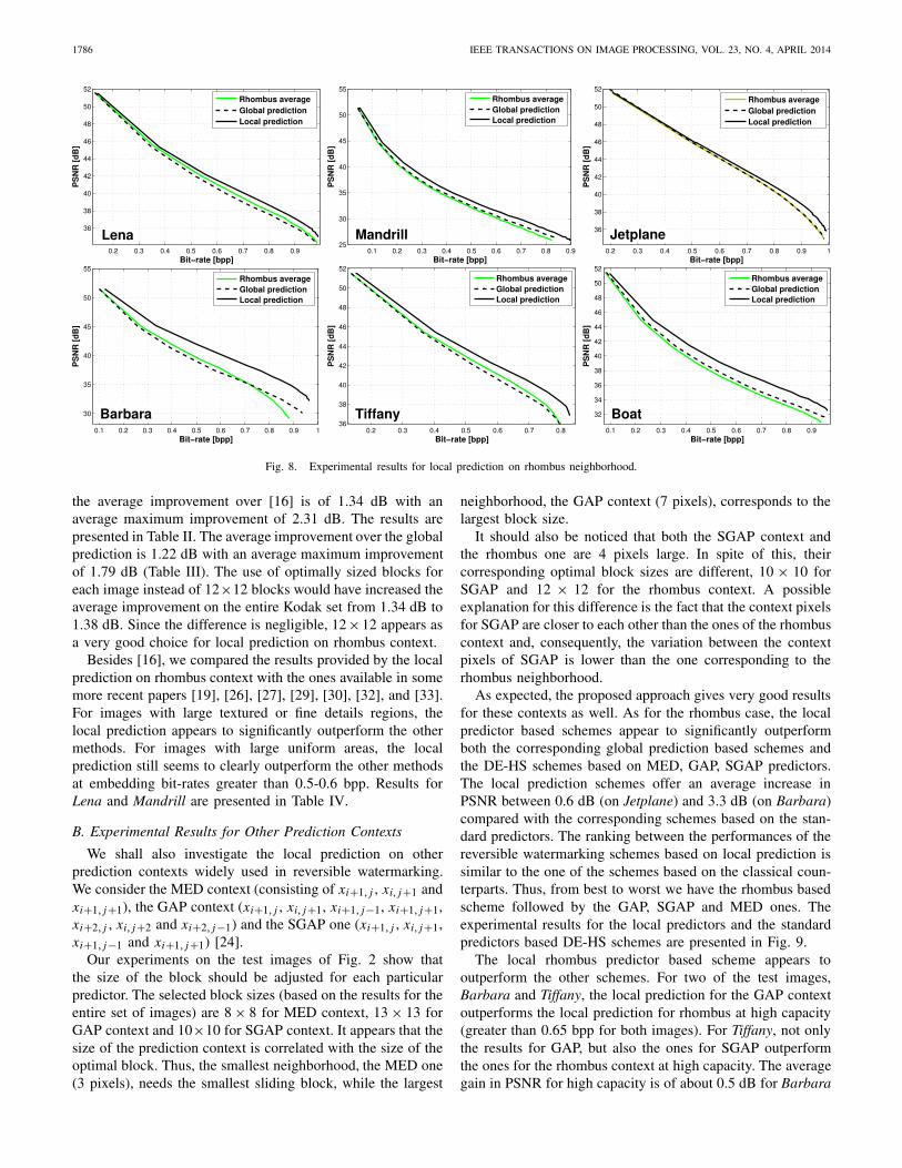
Let us further consider the local prediction with the fol-lowing features: rhombus context plus constant term, thecurrent pixel estimated with equation (10) and the compu-tation performed within a 12 × 12 sliding block. The DE-HSscheme based on local prediction is compared with the globalprediction scheme on rhombus context and with the state ofthe art scheme of [16]. The experimental results for the testimages of Fig. 1 are presented in Fig. 8.

The proposed scheme clearly outperforms both the globallinear prediction based scheme and the two-stages scheme

of [16]. The best results are obtained for Barbara. Comparedwith the results of the previously mentioned schemes, theproposed approach provides an average gain in PSNR ofabout 2.5 dB. At high bit-rates (larger than 0.85 bpp), theproposed scheme outperforms the two-stages scheme of [16]by 5.6 dB and offers an increase in bit-rate of 0.08 bpp. Theincrease in bit-rate corresponds to the embedding of an extra21,000 pixels. A significant increase of the bit-rate appears forMandrill (0.07 bpp) and for Tiffany (0.036 bpp) as well.

The results are also very good for Boat. One gets an averagegain in PSNR of 2 dB compared with [16] and of 1.8 dBcompared with the global prediction scheme. Good resultsare obtained for Mandrill and for Tiffany. For Mandrill, theproposed scheme outperforms [16] by 1.3 dB and the simpleglobal prediction by 1.05 dB. For Tiffany, one gets a gain of0.9 dB compared with [16] and of 1.15 dB compared with theglobal prediction scheme.

For the last two test images, Lena and Jetplane, the increasein PSNR is still easily noticeable, but not as large as onthe other images. We have on Lena an increase of 0.55 dBcompared with the scheme of [16] and of 0.65 dB comparedwith the results provided by the global prediction basedscheme. Finally, for Jetplane, compared with the results of [16]and of the global prediction based scheme, an improvementof 0.5 dB is obtained.

As it can be seen in Fig. 8, the scheme based on the globalpredictor outperforms the rhombus interpolation of [16] onlyon Mandrill and on Boat. As previously mentioned, the mainadvantage of the proposed scheme is the ability to adapt tothe local context of each individual pixel. This can be seenon Barbara where the patterns are clear, at least to the humaneye: a rhombus pattern for the table cloth and stripes for theclothes. Because of the viewing angle and of the creases inthe cloth, the orientations of the stripes vary. Thus, the clotharound the head is a very good example: the lines, slantedto the left, rotate clockwise as we get to the right, wherethey are almost vertical. At the right of the vertical stripes,there are horizontal ones as well. For this type of regionsthe ability to only use the closest pixels for generating thepredictor is crucial, since the patterns change quickly, affectingthe prediction coefficients obtained from large blocks. Thisalso explains the good results on the other textured images,like Mandrill and Boat. On the other end of the spectrum, wehave Jetplane, an image with large uniform areas, ideal forthe rhombus average. The uniform areas are correctly solvedby the proposed scheme as well, but one cannot expect muchimprovement compared with the simple average. Of course,there are also contours and more complex areas, like themountains, where the local prediction gives better results.The case of Lena is rather similar to the one of Jetplane.One has rather large uniform areas where the simple averageperforms well. Because of this, we have a smaller increase inperformance when compared with the other test images.

Next, we tested the rhombus local prediction scheme onthe Kodak graylevel test images and we compared our resultswith the ones of [16] and those of global prediction. Theimprovements are rather similar with the ones obtained forthe classical graylevel test images. On the entire Kodak set,


Fig. 8. Experimental results for local prediction on rhombus neighborhood.

the average improvement over [16] is of 1.34 dB with anaverage maximum improvement of 2.31 dB. The results arepresented in Table II. The average improvement over the globalprediction is 1.22 dB with an average maximum improvementof 1.79 dB (Table III). The use of optimally sized blocks foreach image instead of 12×12 blocks would have increased theaverage improvement on the entire Kodak set from 1.34 dB to1.38 dB. Since the difference is negligible, 12×12 appears asa very good choice for local prediction on rhombus context.

Besides [16], we compared the results provided by the localprediction on rhombus context with the ones available in somemore recent papers [19], [26], [27], [29], [30], [32], and [33].For images with large textured or fine details regions, thelocal prediction appears to significantly outperform the othermethods. For images with large uniform areas, the localprediction still seems to clearly outperform the other methodsat embedding bit-rates greater than 0.5-0.6 bpp. Results forLena and Mandrill are presented in Table IV.

B. Experimental Results for Other Prediction Contexts

We shall also investigate the local prediction on otherprediction contexts widely used in reversible watermarking.We consider the MED context (consisting of xi+1, j , xi, j+1 andxi+1, j+1), the GAP context (xi+1, j , xi, j+1, xi+1, j−1, xi+1, j+1,xi+2, j , xi, j+2 and xi+2, j−1) and the SGAP one (xi+1, j , xi, j+1,xi+1, j−1 and xi+1, j+1) [24].

Our experiments on the test images of Fig. 2 show thatthe size of the block should be adjusted for each particularpredictor. The selected block sizes (based on the results for theentire set of images) are 8 × 8 for MED context, 13 × 13 forGAP context and 10×10 for SGAP context. It appears that thesize of the prediction context is correlated with the size of theoptimal block. Thus, the smallest neighborhood, the MED one(3 pixels), needs the smallest sliding block, while the largest

neighborhood, the GAP context (7 pixels), corresponds to thelargest block size.

It should also be noticed that both the SGAP context andthe rhombus one are 4 pixels large. In spite of this, theircorresponding optimal block sizes are different, 10 × 10 forSGAP and 12 × 12 for the rhombus context. A possibleexplanation for this difference is the fact that the context pixelsfor SGAP are closer to each other than the ones of the rhombuscontext and, consequently, the variation between the contextpixels of SGAP is lower than the one corresponding to therhombus neighborhood.

As expected, the proposed approach gives very good resultsfor these contexts as well. As for the rhombus case, the localpredictor based schemes appear to significantly outperformboth the corresponding global prediction based schemes andthe DE-HS schemes based on MED, GAP, SGAP predictors.The local prediction schemes offer an average increase inPSNR between 0.6 dB (on Jetplane) and 3.3 dB (on Barbara)compared with the corresponding schemes based on the stan-dard predictors. The ranking between the performances of thereversible watermarking schemes based on local prediction issimilar to the one of the schemes based on the classical coun-terparts. Thus, from best to worst we have the rhombus basedscheme followed by the GAP, SGAP and MED ones. Theexperimental results for the local predictors and the standardpredictors based DE-HS schemes are presented in Fig. 9.

The local rhombus predictor based scheme appears tooutperform the other schemes. For two of the test images,Barbara and Tiffany, the local prediction for the GAP contextoutperforms the local prediction for rhombus at high capacity(greater than 0.65 bpp for both images). For Tiffany, not onlythe results for GAP, but also the ones for SGAP outperformthe ones for the rhombus context at high capacity. The averagegain in PSNR for high capacity is of about 0.5 dB for Barbara


TABLE II

GAIN ON KODAK SET OF LOCAL PREDICTORS BASED SCHEMES WITH RESPECT TO CLASSICAL COUNTERPARTS BASED ONES

TABLE III

GAIN ON KODAK SET OF LOCAL PREDICTORS BASED SCHEMES WITH RESPECT TO GLOBAL PREDICTOR BASED ONES

and of 0.27 dB for Tiffany. For capacities lower than 0.65 bppthe results are inferior to the ones obtained with the rhombusneighborhood.

It is interesting to compare the local prediction basedschemes for MED, GAP and SGAP contexts with the schemeof [16] based on the average on rhombus. On three test images,


TABLE IV

PSNR VERSUS BIT-RATE: COMPARISONS WITH SOME RECENT RESULTS

Fig. 9. Experimental results for the classic predictors and the proposed local linear prediction (LP) with different neighborhoods.

(Barbara, Tiffany and Boat), all the local predictors basedschemes outperform [16]. The weakest of the three, the MEDcontext based one, provides an average increase in PSNR of1.4 dB for Barbara, 0.3 dB for Tiffany and 1.2 dB for Boat.On two images, Lena and Mandrill, the results for the MEDcontext and, at low capacities, for GAP and SGAP contexts aswell, overlap with those from [16]. Finally, on Jetplane neitherof the three local predictors outperforms [16]. On the otherhand, the results of [16] outperform the ones of the classicalMED, GAP or SGAP based schemes.

We finally tested the local prediction with the MED, SGAPand GAP context on the Kodak image set. The comparisonwith the fixed prediction based schemes is presented in Table IIand the one with global prediction in Table III. The local pre-diction scheme outperforms its fixed and global counterpartson the entire set, regardless of the pixel context. A comparisonof the results of Tables II and III shows that the schemes based

on rhombus, MED and SGAP are slightly outperformed by theones based on global predictors. The exception is providedby the case of GAP where the fixed predictor based schemeoutperforms with an average of 0.68 dB the one based on theglobal predictor.

The proposed local prediction based schemes for MED,SGAP and GAP contexts can outperform the standard rhombusbased scheme of [16]. The average gain on the entire Kodakset versus [16] is 0.08 dB for LP MED, 0.21 dB for LP SGAPand 0.05 dB for LP GAP. LP MED offers a maximum averageimprovement of 2 dB (image 8), but can also bring a loss ofat most 1.08 dB (image 18). For LP SGAP the maximumimprovement is 2.05 dB (image 8) and the loss is at most1.02 dB (image 18). LP GAP brings a maximum improvementof 1.83 dB (image 8) and a possible loss of at most 1.1 dB(image 13). As expected, the LP scheme based on rhom-bus context outperforms the other three LP based schemes.


It should be noticed that the LP scheme based on rhombusoperates in a single stage in raster-scan order, not in two stagesas the one of [16].

The results presented above have been obtained by using8 × 8 blocks for LP MED, 10 × 10 blocks for LP SGAPand 13 × 13 blocks for LP GAP. Just as it was previouslyobserved on the rhombus based context, the use of optimalsized blocks for each image provides only negligible averageimprovements. More precisely, on the entire set one gets anextra 0.05 dB for MED, 0.03 dB for SGAP and 0.02 dBfor GAP.

C. Mathematical Complexity

Next, we investigate the extra cost required by the localprediction compared with the classical global LS prediction forthe same prediction context. As above, let N × M , B × B andk be the sizes of the image, the block for predictor computationand the prediction context, respectively. For simplicity, oneconsiders N = M . It should be noticed that, for common sizeimages, one has N >> B . In the light of the results presentedabove, one has N > B2 and B > k.

As discussed in Sect. II-B, the computation of a LS predictormeans the solving of an overdetermined system of equations,XX′v = X′y. In the case of a global predictor, the sizes ofthe matrix X and of the vector y are N2 × k and N2 × 1,respectively. The product XX′ needs k2 N2 operations (moreprecisely, k2 N2 multiplications and k2 N2 −k additions). Sincemultiplications are more expensive than the additions, we takeinto account only the multiplications. The product X′y needsonly k N2 operations. After the matrix multiplication step, onegets a simple linear system of k equations with k unknowns.The linear systems of k equations with k unknowns can besolved at a cost of less than k3 operations by using GaussElimination, LU decomposition, etc., (see [34], [35]). Sincek2 N2 is considerably greater than k3, the cost of solving thesystem can be neglected. To conclude, the cost of a globallinear predictor is of about k(k + 1)N2 operations.

The proposed scheme computes a distinct predictor foreach pixel. Instead of solving a single large system of N2

equations, one should solve N2 systems extracted from thelocal B × B blocks. The matrix X and the vector y arereplaced by the matrices Xi,j centered on the central pixeland the corresponding vectors yi,j of sizes B2 × k and B2,respectively. The product of matrices for a single systemdemands k(k + 1)B2 operations. As above, the solving ofthe derived linear system can be neglected. The total cost ofcomputing distinct predictors becomes k(k + 1)B2 N2, i.e. B2

greater than the one of using a global predictor.Since B ∈ [8 − 13], the proposed method appears to be of

about two orders of magnitude more complex than the classicalglobal predictor based reversible watermarking. For instance,for rhombus context, since the entire prediction context isincluded into the 12 × 12 block, the pixels of the first/lastlines and columns are not part of yi,j, just like the centralpixel. Thus, the matrices Xi,j contain only 99 vectors out ofthe 144 of the block. The number of multiplications can bedecreased by updating the products from one block to another.

TABLE V

AVERAGE RUNTIME (IN SECONDS) FOR GLOBAL AND LOCAL

PREDICTION REVERSIBLE WATERMARKING ON 512 × 512

GRAYLEVEL IMAGES

One should replace the effect of the column that leaves theblock with the newly entered one. Theoretically, the updatingof the matrices product can decrease the complexity with aboutone order of magnitude, from B2 to 2B . On the other hand,one has the burden caused by the fact that the current pixelshould not affect the computation.

While the increase of the computational complexity seemsconsiderable, it should be noticed that the cost is still afford-able. Thus, the average execution time of the proposedreversible watermarking scheme on a standard 512 × 512graylevel image using the rhombus context is 12.691 secondsfor the Matlab implementation and 0.554 seconds for theC++ one (using GCC 4.8 of the GNU compiler collection).These results were obtained on a common computer with IntelCore2 Duo E7600 processor at 3.06 GHz, 2 GB MB of RAMand a 64 bit operating system. The average running time forthe different local/global predictors are presented in Table V.The local prediction is computed on blocks of sizes 12 × 12(rhombus), 8 × 8 (MED), 10 × 10 (SGAP), 13 × 13 (GAP).

V. CONCLUSION

The use of local prediction based reversible watermarkinghas been proposed. For each pixel, the least square predictor ina square block centered on the pixel is computed. The schemeis designed to allow the recovery of the same predictor atdetection, without any additional information.

The local prediction based reversible watermarking wasanalyzed for the case of four prediction contexts, namelythe rhombus context and the ones of MED, GAP and SGAPpredictors. The appropriate block sizes have been determinedfor each context. They are 12 × 12 (rhombus), 8 × 8 (MED),10 × 10 (SGAP), 13 × 13 (GAP). The gain obtained byfurther optimization of the block size according to the imageis negligible.

The results obtained so far show that the local predictionbased schemes clearly outperform their global least squareand fixed prediction based counterparts. Among the four localprediction schemes analyzed, the one based on the rhom-bus context provides the best results. The results have beenobtained by using the local prediction with a basic differenceexpansion scheme with simple threshold control, histogramshifting and flag bits.

REFERENCES

[1] M. Goljan, J. Fridrich, and R. Du, “Distortion-free data embedding forimages,” Inf. Hiding, vol. 2137, pp. 27–41, Apr. 2001.

[2] M. U. Celik, G. Sharma, A. M. Tekalp, and E. Saber, “Losslessgeneralized LSB data embedding,” IEEE Trans. Imag. Process., vol. 14,no. 2, pp. 253–266, Feb. 2005.


[3] Z. Ni, Y. Q. Shi, N. Ansari, and W. Su, “Reversible data hiding,”IEEE Trans. Circuits Syst. Video Technol., vol. 16, no. 3, pp. 354–362,Mar. 2006.

[4] C. C. Lin, W. L. Tai, and C. C. Chang, “Multilevel reversible datahiding based on histogram modification of difference images,” PatternRecognit., vol. 41, no. 12, pp. 3582–3591, 2008.

[5] P. Tsai, Y.-C. Hu, and H.-L. Yeh, “Reversible image hiding scheme usingpredictive coding and histogram shifting,” Signal Process., vol. 89, no. 6,pp. 1129–1143, 2009.

[6] L. Luo, Z. Chen, M. Chen, X. Zeng, and Z. Xiong, “Reversible imagewatermarking using interpolation technique,” IEEE Trans. Inf., ForensicsSecurity, vol. 5, no. 1, pp. 187–193, Mar. 2010.

[7] W. Hong, T.-S. Chen, and C.-W. Shiu, “Reversible data hiding for highquality images using modification of prediction errors, J. Syst. Softw.,vol. 82, no. 11, pp. 1833–1842, 2009.

[8] C. Wang, X. Li, and B. Yang, “Efficient reversible image watermarkingby using dynamical prediction-error expansion,” in Proc. 17th ICIP,2010, pp. 3673–3676.

[9] J. Tian, “Reversible data embedding using a difference expansion,”IEEE Trans. Circuits Syst. Video Technol., vol. 13, no. 8, pp. 890–896,Aug. 2003.

[10] A. M. Alattar, “Reversible watermark using the difference expansion ofa generalized integer transform,” IEEE Trans. Image Process., vol. 13,no. 8, pp. 1147–1156, Aug. 2004.

[11] D. M. Thodi and J. J. Rodriguez, “Expansion embedding techniques forreversible watermarking,” IEEE Trans. Image Process., vol. 16, no. 3,pp. 721–729, Mar. 2007.

[12] G. Coatrieux, W. Pan, N. Cuppens-Boulahia, F. Cuppens, and C. Roux,“Reversible watermarking based on invariant image classification anddynamic histogram shifting,” IEEE Trans. Inf., Forensics Security, vol. 8,no. 1, pp. 111–120, Jan. 2013.

[13] D. Coltuc and J.-M. Chassery, “Very fast watermarking by reversiblecontrast mapping,” IEEE Signal Process. Lett., vol. 15, no. 4,pp. 255–258, Apr. 2007.

[14] A. Tudoroiu and D. Coltuc, “Local map versus histogram shifting forprediction error expansion reversible watermarking,” in Proc. ISSCS,2013, pp. 1–4.

[15] L. Kamstra and H. J. A. M. Heijmans, “Reversible data embeddinginto images using wavelet techniques and sorting,” IEEE Trans. ImageProcess., vol. 14, no. 12, pp. 2082–2090, Dec. 2005.

[16] V. Sachnev, H. J. Kim, J. Nam, S. Suresh, and Y. Q. Shi, “Reversiblewatermarking algorithm using sorting and prediction,” IEEE Trans.Circuits Syst. Video Technol., vol. 19, no. 7, pp. 989–999, Jul. 2009.

[17] B. Ou, X. Li, Y. Zhao, R. Ni, and Y. Shi, “Pairwise prediction-errorexpansion for efficient reversible data hiding,” IEEE Trans. ImageProcess., vol. 22, no. 12, pp. 5010–5021, Dec. 2013.

[18] Y. Hu, H.-K. Lee, and J. Li, “DE-based reversible data hiding withimproved overflow location map,” IEEE Trans. Circuits Syst. VideoTechnol., vol. 19, no. 2, pp. 250–260, Feb. 2009.

[19] X. Li, B. Yang, and T. Zeng, “Efficient reversible watermarking basedon adaptive prediction-error expansion and pixel selection,” IEEE Trans.Image Process., vol. 20, no. 12, pp. 524–3533, Dec. 2011.

[20] M. Weinberger, G. Seroussi, and G. Sapiro, “The LOCO-I lossless imagecompression algorithm: Principles and standardization into JPEG-LS,”IEEE Trans. Image Process., vol. 9, no. 8, pp. 1309–1324, Aug. 2000.

[21] X. Wu and N. Memon, “Context-based, adaptive, lossless image coding,”IEEE Trans. Commun., vol. 45, no. 4, pp. 437–444, Apr. 1997.

[22] M. Fallahpour, “Reversible image data hiding based on gradient adjustedprediction,” IEICE Electron. Exp., vol. 5, no. 20, pp. 870–876, 2008.

[23] M. Chen, Z. Chen, X. Zeng, and Z. Xiong, “Reversible data hidingusing additive prediction-error expansion,” in Proc. 11th ACM WorkshopMultimedia Security, 2009, pp. 19–24.

[24] D. Coltuc, “Improved embedding for prediction based reversible water-marking,” IEEE Trans. Inf. Forensics Security, vol. 6, no. 3, pp. 873–882,Sep. 2011.

[25] I.-C. Dragoi and D. Coltuc, “Improved rhombus interpolation forreversible watermarking by difference expansion,” in Proc. 20th Eur.Conf. Signal. Process., 2012, pp. 1688–1692.

[26] B. Ou, X. Li, Y. Zhao, and R. Ni, “Reversible data hiding based on PDEpredictor,” J. Syst. Softw., vol. 86, no. 10, pp. 2700–2709, 2012.

[27] X. Li, B. Li, B. Yang, and T. Zeng, “General framework to histogram-shifting-based reversible data hiding,” IEEE Trans. Image Process.,vol. 22, no. 6, pp. 2181–2191, Jun. 2013.

[28] D. Coltuc and I.-C. Dragoi, “Context embedding for raster-scan rhombusbased reversible watermarking,” in Proc. 1st ACM Workshop Inf. HidingMultimedia Security, 2013, pp. 215-220,

[29] W. Zhang, X. Hu, X. Li, and N. Yu, “Recursive histogram modification:Establishing equivalency between reversible data hiding and losslessdata compression,” IEEE Trans. Image Process., vol. 22, no. 7,pp. 2775–2785, Jul. 2013.

[30] W. Zhang, B. Chen, and N. Yu, “Improving various reversible datahiding schemes via optimal codes for binary covers,” IEEE Trans. ImageProcess., vol. 21, no. 6, pp. 2991–3003, Jun. 2012.

[31] M. Arsalan, S. A. Malik, and A. Khan, “Intelligent reversible water-marking in integer wavelet domain for medical images,” J. Syst. Softw.,vol. 85, no. 4, pp. 883–894, Apr. 2012.

[32] H.-T. Wu and J. Huang, “Reversible image watermarking on predictionerrors by efficient histogram modification,” Signal Process., vol. 92,no. 12, pp. 3000–3012, 2012.

[33] X. Zhang, “Reversible data hiding with optimal value transfer,” IEEETrans. Multimedia, vol. 15, no. 2, pp. 316–325, Feb. 2013.

[34] W. H. Press, S. S. Teukolsky, W. T. Vetterling, and B. P. Flannery,Numerical Recipes in C: The Art of Scientific Computing. Cambridge,MA, USA: Wellesley-Cambridge, 1992.

[35] G. H. Golub and C. F. Van Loan, Matrix Comput.. Baltimore, MD, USA:Johns Hopkins Univ., 1996.

Ioan-Catalin Dragoi received the Diploma of Engi-neer degree in applied electronics and the master’sdegree in advanced telecommunications, informa-tion processing, and transmission systems from theValahia University of Targoviste, Romania, in 2010and 2012, respectively, where he is currently pursu-ing the Ph.D. degree with the Doctoral School ofEngineering. His current research interests includeimage processing and watermarking.

Dinu Coltuc received the Diploma of Engineer andPh.D. degrees in electronics and telecommunica-tions from the Politechnica University of Bucharest,Romania, in 1982 and 1997, respectively. He iscurrently a Professor of Electrical Engineering, Elec-tronics and Information Technology School, ValahiaUniversity of Targoviste, Romania. He is the Direc-tor with the Doctoral School of Engineering andthe Director with the Research Center for ElectricalEngineering, Electronics and Information Technol-ogy, Valahia University of Targoviste. His current

research interests include in the areas of image and signal processing,watermarking, image enhancement, and fast algorithms.

Documents

Local-Prediction-Based Difference Expansion Reversible Watermarking