Local Pivotal Methods for Large Surveys

Jonathan J. Lisic ∗ Nathan B. Cruze ∗

AbstractThe local pivotal method described provides a method to draw a spatially balanced sample for

an arbitrary number of dimensions reducing the need for complex stratification for spatial surveys.Unfortunately, due to its quadratic run-time the local pivotal method has been restricted to popula-tions with less than one million sampling units. In this paper, one alternative implementation andtwo approximations of this method are presented. The first uses a k-d tree data structure to imple-ment the local pivotal method, which results in a sub-quadratic run-time. The second two methodsrelax the nearest-neighbor requirement in exchange for a further reduction in computational timethrough approximate nearest-neighbors. In this paper, an analysis of the effects of approximatingspatial neighborhoods and a comparison of run-times between the proposed methods and existingimplementations are provided for both simulated and real area frames.

Key Words: Nearest-Neighbor, Sampling, Spatial

1. Introduction

Tobler’s First Law of Geography, Tobler (1970), states that “everything is related to every-thing else, but near things are more related than distant things.” This is true for spatiallyclose sampling units such as businesses, farms, and households; where neighboring sam-pling units are likely to have characteristics that exhibit spatial correlation. Because spatialcorrelation lowers the effective sample size when sampling units are close together (seeCressie, 1993), care should be taken to ensure that sampling units are well spread. Severalproposed methods address this specific issue: the local pivotal method (LPM) (see Graf-strom et al., 2012), spatially correlated Poisson sampling (SCPS) (see Grafstrom, 2012), thegeneralized random-tessellation stratified method (GRTS) (see Stevens Jr and Olsen, 2004),and the draw-by-draw sampling excluding the selection of contiguous units (DDSESCU)(see Fattorini, 2006).

Unfortunately, none of these methods scale well to large populations. Both SCPS andLPM require nearest-neighbor searches, yielding quadratic computational complexity asseen in Grafstrom et al. (2012) and Grafstrom (2012) respectively. This particular problemis apparent in Grafstrom et al. (2014), where LPM is approximated to sample from a frameof 818,017 sampling units.

GRTS relies heavily on a data structure known as a quadtree. Quadtrees have excellentproperties with respect to retrieving data, but can be computationally intensive to construct.This limitation can be seen in the R package spsurvey (see Kincaid and Olsen, 2015) wherethe number of levels of a tree are limited to 11, or a little over 4 million possible samplingunits. DDSESCU, the drawn-by-drawn method, uses simulation to determine inclusionprobabilities. This method is not usable for large population sizes due to the low probabilityof re-drawing the same unit.

This paper focuses on reducing the computational complexity of LPM, although a sim-ilar approach could be applied to SCPS. The approach taken here is through the use ofk-dimensional trees (k-d trees) to accelerate nearest-neighbor searches. Section 2 of thispaper provides background on LPM and k-d trees. Section 3 introduces an approximation

∗United States Department of Agriculture, National Agricultural Statistics Service, 1400 IndependenceAvenue SW, Washington, DC 20250

to nearest-neighbor searching in k-d trees, which provides a greater decrease in computa-tion complexity. Section 4 presents algorithms for both exact and approximate LPM usingk-d trees. Simulated and empirical results for the accelerated LPM algorithm and its ap-proximations are provided in Section 5. Finally, a discussion of the results and possiblefuture work are provided in Section 6.

2. Background

The method presented in this paper is built on two key ideas, the local pivotal method andk-dimensional trees. LPM provides a method to create well spread or spatially balancedsamples (Figure 1). This method creates spatial balanced samples by locally aggregat-ing inclusion probabilities from neighboring sampling units, lowering the probability thatadjacent sampling units are sampled. k-d trees assist this method by providing a computa-tionally efficient means to identify neighboring sampling units.

Before introducing the LPM, it is important to first define spatial balance. In this paperspatial balance follows the definition provided by Stevens Jr and Olsen (2004),

B =∑i∈S

−1 +∑j∈Ni

πj

2

(1)

whereS = sample of size n from a population U of size N ;Ni = spatial neighborhood (Voronoi tessellation about sampled point i);πi = Pr (i ∈ S), the first order inclusion probability in sample S ⊂ U .

Necessarily,∑i∈U πi = n and 1 ≥ πi > 0 ∀i ∈ U .

B is bounded on the interval [0, n(n − 1)). The lower bound occurs when the sampleis perfectly balanced; the sum of first order inclusion probabilities over each tessellate isone. The upper bound occurs under two conditions. First, the sampling weights for N − nmembers of the frame have a small inclusion probability π∗, identified asA, and nmembersof the frame have inclusion probabilities close to one, identified as A′. Furthermore, thesets A and A′ are mutually disjoint; A ∪ A′ = U and A ∩ A′ = ∅. Second, the membersof A are sufficiently isolated in the spatial support from A′ such that there exists a samplewith a tessellate containing all n members of A′. If this specific sample is drawn, then asingle tessellate has a sum of inclusion probabilities over Ni close to n, where i ∈ A′. Allother tessellates have sums over Ni close to zero, i ∈ A. In the limit, as π∗ goes to zero,then B goes to n− 1 + (n− 1)2 = n(n− 1). This limit can be verified through Lagrangeoptimization over πi, where −B is minimized with the constraint

∑i∈U πi − n = 0.

An intuitive case for this measure of balance occurs when the first order inclusion prob-abilities are equal and the sampling units in the population are evenly spread across the spa-tial domain. In this case, if each tessellate has the same area, then B is zero; a consequenceof sampled points being well spread. Although it should be noted that B can be zero whenthe sampled points are adjacent to each other, as in the case of the sampled points forminga circle at the center of a disc-shaped spatial region. However, in practice this later case israre.

k-d trees, like the previously mentioned tessellates, partition the spatial domain into aset of mutually disjoint and connected regions. In the case of k-d trees the partitioning isdone through recursively bisecting the spatial domain by a univariate statistic such as a me-dian. The univariate statistic is applied to each dimension of the k-d tree either by iteratingover the index of the dimensions or through a heuristic, such as picking the dimension withthe largest marginal variance. This partitioning algorithm allows for the construction of a

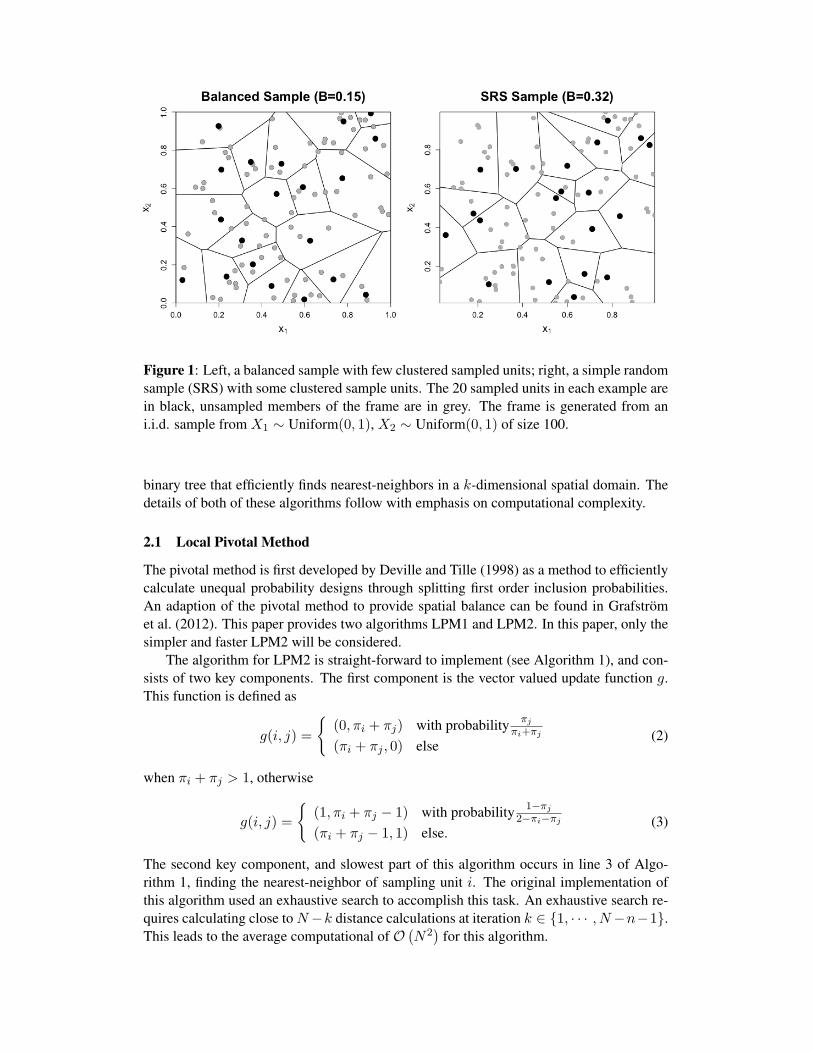
Figure 1: Left, a balanced sample with few clustered sampled units; right, a simple randomsample (SRS) with some clustered sample units. The 20 sampled units in each example arein black, unsampled members of the frame are in grey. The frame is generated from ani.i.d. sample from X1 ∼ Uniform(0, 1), X2 ∼ Uniform(0, 1) of size 100.

binary tree that efficiently finds nearest-neighbors in a k-dimensional spatial domain. Thedetails of both of these algorithms follow with emphasis on computational complexity.

2.1 Local Pivotal Method

The pivotal method is first developed by Deville and Tille (1998) as a method to efficientlycalculate unequal probability designs through splitting first order inclusion probabilities.An adaption of the pivotal method to provide spatial balance can be found in Grafstromet al. (2012). This paper provides two algorithms LPM1 and LPM2. In this paper, only thesimpler and faster LPM2 will be considered.

The algorithm for LPM2 is straight-forward to implement (see Algorithm 1), and con-sists of two key components. The first component is the vector valued update function g.This function is defined as

g(i, j) ={

(0, πi + πj) with probability πj

πi+πj

(πi + πj , 0) else(2)

when πi + πj > 1, otherwise

g(i, j) ={

(1, πi + πj − 1) with probability 1−πj

2−πi−πj

(πi + πj − 1, 1) else.(3)

The second key component, and slowest part of this algorithm occurs in line 3 of Algo-rithm 1, finding the nearest-neighbor of sampling unit i. The original implementation ofthis algorithm used an exhaustive search to accomplish this task. An exhaustive search re-quires calculating close toN−k distance calculations at iteration k ∈ {1, · · · , N−n−1}.This leads to the average computational of O

(N2) for this algorithm.

Algorithm 1 LPM2 Algorithm.1: while length (U∗) > 0 do2: Randomly select sampling unit i ∈ U∗ with uniform probability.3: Set j to the nearest-neighbor of i in U∗.4: Set (πi, πj) := g (πi, πj).5: Set U∗ := U∗\{k ∈ {i, j} : πk ∈ {0, 1}}.6: end while

Simple k-d Tree

x·,1 < 0.504

x·,2 < 0.427

A1

x·,2 ≥ 0.427

A2

x·,1 ≥ 0.504

x·,2 < 0.582

A3

x·,2 ≥ 0.582

A4

Figure 2: k-d tree node structure with depth = 2 applied to the population in Figure 1.

2.2 k-Dimensional Trees

Nearest-neighbors algorithms are integral in common statistical techniques such as k-nearest-neighbor clustering and calculation of high dimensional kernel density estimates. In both ofthese cases, k-d trees and variants provide a data structure that allows for nearest-neighborqueries with average computational complexity of O (log(n)) (see Muja and Lowe, 2014and Lang et al., 2005). This search time is lower than the linear search used in the originalLPM2 algorithm, but comes at the expense of building the k-d tree. k-d tree constructionhasO (n log(n)) computational complexity. Since computational complexity is defined upto a constant, the average computational complexity for tree construction and n queriesagainst the tree is also O (n log(n)). Therefore, even with tree construction the averagecomputational complexity of the n k-d tree searches is much lower than the quadratic com-putational complexity of the linear search.

k-d trees partition a set of k-dimensional points into a set of mutually exclusive sub-sets. This partitioning is done by splitting the original k-dimensional space along a singledimension at the median or other statistic calculated from the points in the space. Subse-quent applications of this partitioning are performed individually on the resulting partitions,choosing a different dimension at each iteration. The choice of dimension can be made bysimply iterating over each dimension repeatedly, or by selecting the dimension based ona heuristic such as the largest marginal variance. Tree construction terminates when thenumber of points in each subspace is less than or equal to a fixed number of nodes, wherethe number is set a priori. A graphical view of a k-d tree applied to data in Figure 1 withleaf node size m equal to 25 is provided in Figure 2 with the partitioning of the spatialsupport depicted in Figure 3. Further partitioning by the algorithm can be seen in Figure 4with m equal to 13 and 7.

An algorithm to build a k-d tree-based on iterating through dimensions is detailed asAlgorithm 2. In this algorithm the set of k-dimensional points X are indexed by the indexI. During each split, the sets and indexes are split between the child nodes. Note that, thealgorithm provided is known as a leaf based k-d tree since all points are stored in the leafsas opposed to within the nodes of the tree, non-leaf based approaches are not pursued inthis research.

Figure 3: Labeled partitions of a k-d tree with max leaf node size ofm = 25 from Figure 2.A query point (labeled 1) and its nearest-neighbors in A1 (labeled point 3) and A2 (labeledpoint 2) are circled.

Once a tree is constructed it can be queried to find neighbors. In the case of LPMand related methods, the query of interest is to find the nearest-neighbor of a point in thek-d tree. Since the point of interest is within the k-d tree, care needs to be taken to avoidreturning the point queried. This can be avoided by performing an index check beforecomparing distances; if the index being queried matches the point to be compared, thenthis point is skipped. An algorithm that will return the nearest-neighbor of a point in the k-d tree is provided as Algorithm 3. To simplify this algorithm, no attempt is made to handleties between distances. Such ties are common if applied to pixel data, and can be handledthrough reservoir sampling (see Sunter, 1977).

The search algorithm goes through three phases to find the nearest-neighbor for a querypoint in the tree. The first phase is a depth first search to find a partition of space thatcontains points close to the query point. Once the first leaf node is encountered phase twobegins. In phase two, each point in the partition associated with the leaf node is comparedto the query point. Care is taken to ensure comparisons are not done between the querypoint and itself. If a point is found closer to the point being queried than any prior pointevaluated, it is set as the current nearest-neighbor and the distance between this point andthe queried point is retained. After all points in the partition of point have been compared,the tree will backtrack to other nodes in the tree. However, in this third phase, only nodesthat could feasibly lead to a point sufficiently close to the query point are considered. Thisfeasibility is determined through the univariate median used for splitting in the k-d tree. Ifthe distance between the query point and the univariate median for a given node is greaterthan the current distance, this node and all of its children will not be visited. This greatly

Figure 4: Labeled partitions of a k-d trees with max leaf node size of m = 13 (left) andm = 7 (right) from Figure 3.

Algorithm 2 Algorithm to build a k-d tree for a k-dimensional data set.1: initialize:

Index the points in the set X with Ii← 1

2: procedure KDTREE(I,i)3: Create new node A, with attributes left, right, median, and data.4: if length (I) > m then5: Split I into Il and Ir by the median of dimension i modulo k plus one.6: Set A’s median to the split point.7: Set A’s left child to KDTREE(Il,i+ 1).8: Set A’s right child to KDTREE(Ir,i+ 1).9: else

10: Set A’s data to I.11: end if12: return A13: end procedure

reduces the number of nodes to explore. These three phases are revisited until all viablenodes are traversed.

As an illustrative example, a query to find the nearest-neighbor of point v = (0.413, 0.437)in a tree with leaf nodes of size 25 is provided. This point is identified in Figure 3 as point1, and the tree in Figure 5 identifies the nodes visited in the query of this tree in bold. Inthe first phase the left node is selected since the first element of v, 0.413, is less than theunivariate median in the first dimension of X; the right node is selected next since the sec-ond element of v is greater than or equal to 0.427. Phase two begins with the exhaustivenearest-neighbor search of all points in the subset of the partition labeled A2; this searchconcludes with identification of the nearest-neighbor, point (0.330, 0.505) with distance0.011 (identified as point 2). In phase three, the distance between the second element ofv and the univariate median of the second dimension is calculated as 0.0001. Since thisdistance is less than the current distance of 0.011, partition A1 is also explored resultingin a nearest-neighbor of (0.420, 0.352) with distance 0.007 (identified as point 3). Finally

Algorithm 3 Algorithm to query a k-d tree for the nearest-neighbor using the L2 norm.1: initialize:

Index the points in the set X with IQuery for index a ∈ Iy ← xa ∈ Xdist←∞

2: procedure SEARCH(A,i,(neighbor, dist))3: if A’s median is defined. then4: Set j to i modulo k.5: q ← A′s median6: if yj ≤ q then7: (neighbor, dist)← SEARCH(Al,i+ 1,(neighbor, dist)).8: if (yj − q)2 < dist then9: (neighbor, dist)← SEARCH(Ar,i+ 1,(neighbor, dist)).

10: end if11: else12: (neighbor, dist)← SEARCH(Ar,i+ 1,(neighbor, dist)).13: if (yj − q)2 < dist then14: (neighbor, dist)← SEARCH(Al,i+ 1,(neighbor, dist)).15: end if16: end if17: else18: for b in A’s data do19: z ← xb20: if a 6= b then21: if ||y − z||22 < dist then22: dist← ||y − z||2223: neighbor← b24: end if25: end if26: end for27: end if28: return (neighbor, dist)29: end procedure

we enter phase 3 again and the distance is calculated between the first element of v andthe univariate median of the first dimension, here the distance is 0.008 exceeding our priorminimum distance of 0.007. Since the minimum distance is exceeded there are no checksdone on the right hand side of the tree. At this point the query terminates because there areno further nodes to check. The point (0.420, 0.352) is returned as the nearest-neighbor.

3. Approximate Nearest-Neighbors

The nearest-neighbor literature also considers approximate nearest-neighbors (ANN) (seeArya et al., 1998) as a means to accelerate searches by sacrificing the requirement forclosest neighbors. Instead of closest neighbors, the requirement is replaced with the closestneighbors found in a fixed amount of time or within a minimum distance. This form ofapproximation can be useful in application to LPM2, by sacrificing balance for speed. Inthis research, two methods of ANN are considered. The first is time-based. In this method

Simple k-d Tree

x·,1 < 0.504

x·,2 < 0.427

A1

x·,2 ≥ 0.427

A2

x·,1 ≥ 0.504

x·,2 < 0.582

A3

x·,2 ≥ 0.582

A4

Figure 5: A search for the nearest-neighbor of point (0.413, 0.437) (point 1. in Figure 3).

Simple k-d Tree

x·,1 < 0.504

x·,2 < 0.427

A1

x·,2 ≥ 0.427

A2

x·,1 ≥ 0.504

x·,2 < 0.582

A3

x·,2 ≥ 0.582

A4

Figure 6: A search for the nearest-neighbor of point (0.413, 0.437) (point 1. in Figure 3),using the time-based ANN (leaf check = 1).

the amount of time to find the closest neighbor is fixed, where time is specified as thenumber of partitions (leaf nodes) to check. The second is distance based, where the firstneighbor found that is sufficiently close to the sampled point will be taken as an ANN.

Time-based ANN methods restrict searching for neighbors to a subset of the spatialdomain. This improves the worst case performance of k-d trees (fixing number of leavesto check), avoiding traversals over large portions of the tree. The path taken by a time-based ANN for the prior example is presented in Figure 6. In this example, the maximumnumber of leaves to check is set to one; this returns the point (0.330, 0.505) with distance0.011 instead of the exact nearest-neighbor with distance 0.007. If the maximum numberof leaves to check is set to two or more, we get the same result as the nearest-neighborssearch Figure 5.

Distance-based approximations treat all potential neighbors within a fixed distance asANNs. Unlike the time-based ANN method, this restriction does not necessarily improvethe worst case performance of k-d trees. Instead, if the threshold is set too low an exactnearest-neighbor search will result. To ensure reduced run-time, some knowledge aboutappropriate distances is required.

In general, ties are not handled for values below the threshold. This lack of tie handlingis potentially problematic if the order of evaluation of points in a leaf node are positivelycorrelated with a variable of interest in the population.

The point returned as an ANN can be sensitive to the choice of threshold distance. Inthe case of the population in Figure 3, a threshold of distance 0.008 or higher will onlyexplore the subset A2 as in Figure 6. A threshold distance of 0.008 will return the samevalue as the time-based ANN with leaf check set at one. Likewise, a threshold set at 0.007or lower will provide no reduction in leaf checks and return an exact nearest-neighbor. Inan extreme case, a positive unbound threshold distance will return the first point found,with distance 0.285.

4. k-d Tree Acceleration

Integration of k-d tree-based nearest-neighbor searches in LPM2 is straight forward andallows for additional acceleration for simulation by preserving the tree structure betweendraws. For further performance gains, approximate nearest-neighbors k-d tree searches canbe integrated in the same way. However, there is a trade-off to be made between the qualityof the approximation and speed.

The LPM2 algorithm, Algorithm 1, can be modified to include k-d tree-based acceler-ated queries in two steps. First, a k-d tree must be built based on the points being sampledbefore line 1. Second, line 3 must be replaced with a k-d tree nearest-neighbor search or anapproximate nearest-neighbor search. This modification will provide an exact replicationof the results from the linear search implementation, provided that tied distances are han-dled in the same way. In k-d tree searches, the only additional burden is the cost of storingthe tree in memory; fortunately, the storage requirements for the tree only grows linearlywith respect to the number of points.

For simulations, multiple draws from the same sample do not require rebuilding thetree. This can make ANN searches considerably more desirable than using exact nearest-neighbor searches, since the approximate approach can have lower per-search cost and thetree building cost is amortized as the number of simulations increases.

ANN variants of LPM2 do make a trade-off between spatial balance and computationalburden. By restricting the number of nodes to search, there is a chance that closer pointsmay be ignored. Since there is a non-zero chance of exploring outside the node that thepoint being queried exists in, the joint inclusion probability of any two points remains non-zero. However, the joint inclusion probability can be substantially lowered for points thatare spatially close but on opposite sides of a split that occurs early in tree formation.

5. Comparison of Algorithms

In this section, the performance and spatial balance of these algorithms are compared.This comparison is performed on simulated and real area frames. For simplicity, equalprobability sampling is used for all comparisons. In the simulated cases, all populations arebased on a bivariate uniform distribution of varying size distributed asX1 ∼ Uniform(0, 1)andX2 ∼ Uniform(0, 1), withX1 independent ofX2, and a fixed sample size of 100. As anapplication to real data, the U.S. Census Bureau’s 2010 block data are used. All calculationsare performed using the R package BalancedSampling (see Grafstrom and Lisic, 2016).

To evaluate performance, a comparison of the log run-times is performed between thelinear search and k-d tree implementations of the LPM2 algorithm, followed by a com-parison between the run-times of the nearest-neighbor and ANN k-d tree implementations.Since the ANN variants of LPM2 do not necessarily preserve the nearest-neighbor, a shortexploration of the effect of approximation on balance is performed. In this exploration, acomparison of spatial balance is performed between simple random sample (SRS), LPM2,and LPM2 approximations.

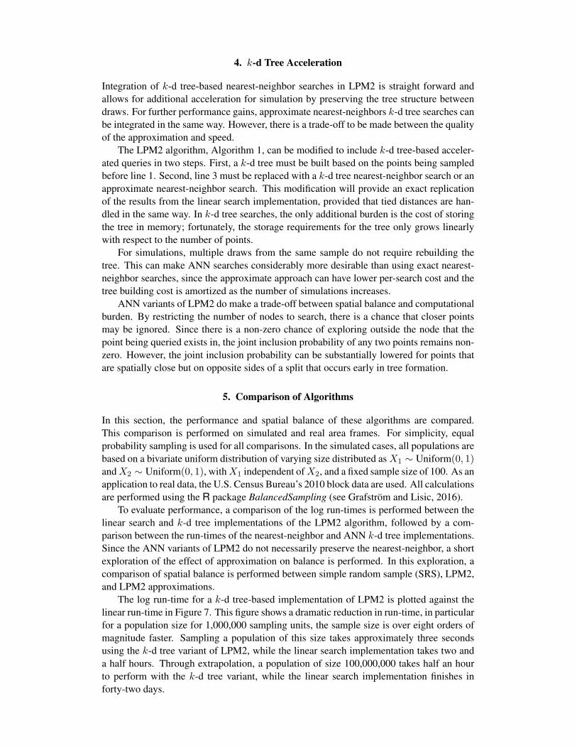
The log run-time for a k-d tree-based implementation of LPM2 is plotted against thelinear run-time in Figure 7. This figure shows a dramatic reduction in run-time, in particularfor a population size for 1,000,000 sampling units, the sample size is over eight orders ofmagnitude faster. Sampling a population of this size takes approximately three secondsusing the k-d tree variant of LPM2, while the linear search implementation takes two anda half hours. Through extrapolation, a population of size 100,000,000 takes half an hourto perform with the k-d tree variant, while the linear search implementation finishes inforty-two days.

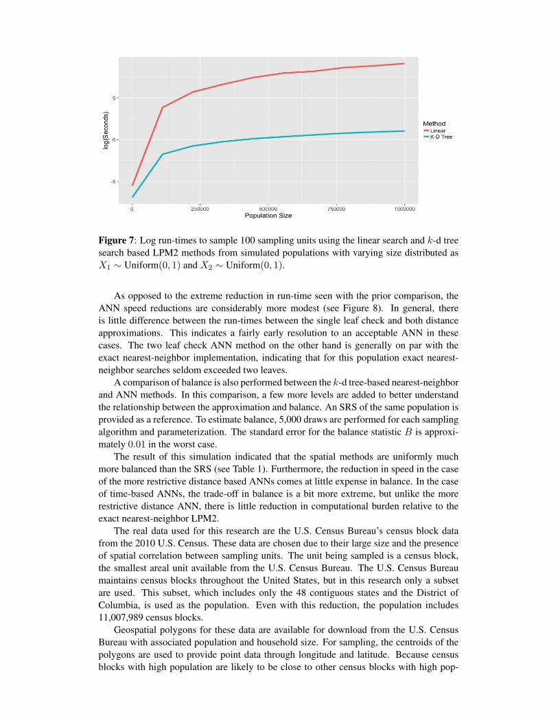
Figure 7: Log run-times to sample 100 sampling units using the linear search and k-d treesearch based LPM2 methods from simulated populations with varying size distributed asX1 ∼ Uniform(0, 1) and X2 ∼ Uniform(0, 1).

As opposed to the extreme reduction in run-time seen with the prior comparison, theANN speed reductions are considerably more modest (see Figure 8). In general, thereis little difference between the run-times between the single leaf check and both distanceapproximations. This indicates a fairly early resolution to an acceptable ANN in thesecases. The two leaf check ANN method on the other hand is generally on par with theexact nearest-neighbor implementation, indicating that for this population exact nearest-neighbor searches seldom exceeded two leaves.

A comparison of balance is also performed between the k-d tree-based nearest-neighborand ANN methods. In this comparison, a few more levels are added to better understandthe relationship between the approximation and balance. An SRS of the same population isprovided as a reference. To estimate balance, 5,000 draws are performed for each samplingalgorithm and parameterization. The standard error for the balance statistic B is approxi-mately 0.01 in the worst case.

The result of this simulation indicated that the spatial methods are uniformly muchmore balanced than the SRS (see Table 1). Furthermore, the reduction in speed in the caseof the more restrictive distance based ANNs comes at little expense in balance. In the caseof time-based ANNs, the trade-off in balance is a bit more extreme, but unlike the morerestrictive distance ANN, there is little reduction in computational burden relative to theexact nearest-neighbor LPM2.

The real data used for this research are the U.S. Census Bureau’s census block datafrom the 2010 U.S. Census. These data are chosen due to their large size and the presenceof spatial correlation between sampling units. The unit being sampled is a census block,the smallest areal unit available from the U.S. Census Bureau. The U.S. Census Bureaumaintains census blocks throughout the United States, but in this research only a subsetare used. This subset, which includes only the 48 contiguous states and the District ofColumbia, is used as the population. Even with this reduction, the population includes11,007,989 census blocks.

Geospatial polygons for these data are available for download from the U.S. CensusBureau with associated population and household size. For sampling, the centroids of thepolygons are used to provide point data through longitude and latitude. Because censusblocks with high population are likely to be close to other census blocks with high pop-

Figure 8: Run-times to sample 100 sample units using k-d tree-based LPM2 methods fromsimulated populations with varying size distributed as X1 ∼ Uniform(0, 1) and X2 ∼Uniform(0, 1).

Table 1: A comparison of the balance statistic calculated from 5,000 draws per algorithmon a simulated population of 10,000 sampling units with sample size 100.

Algorithm BalanceLPM2 0.07

SRS 0.32

k-d Tree TimeLeaf Check

1 2 3 40.10 0.07 0.07 0.07

k-d Tree Dist.Distance

1 0.1 0.01 0.0010.10 0.10 0.09 0.07

ulation, these data exhibit a high degree of spatial correlation between adjacent samplingunits. In this experiment 5,000 samples of size 2,000 are drawn from the entire population.In each draw, a Horvitz-Thompson estimator of the U.S. Population for the 48 contiguousstates is calculated. Owing to limitations of the software, each draw required rebuilding thek-d tree, significantly increasing the run-time.

The results of this simulation are provided in Table 2. In these results, variance relativeto SRS is reduced by 9% for the approximate and 7% for the exact LPM2 sampling. Un-fortunately, the sample variance for these results with 5,000 draws is sufficiently large tomake the differences insignificant at a 5% confidence level. The difference in run-time isfairly insignificant with 45 seconds and 46 seconds for the time and distance based methodsrespectfully, and 58 seconds for the exact method.

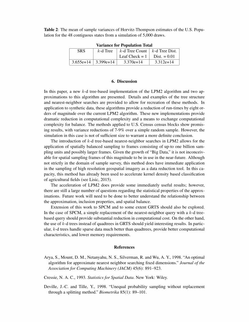
Table 2: The mean of sample variances of Horvitz-Thompson estimates of the U.S. Popu-lation for the 48 contiguous states from a simulation of 5,000 draws.

Variance for Population TotalSRS k-d Tree k-d Tree Count k-d Tree Dist.

Leaf Check = 1 Dist. = 0.013.655e+14 3.399e+14 3.370e+14 3.312e+14

6. Discussion

In this paper, a new k-d tree-based implementation of the LPM2 algorithm and two ap-proximations to this algorithm are presented. Details and examples of the tree structureand nearest-neighbor searches are provided to allow for recreation of these methods. Inapplication to synthetic data, these algorithms provide a reduction of run-times by eight or-ders of magnitude over the current LPM2 algorithm. These new implementations providedramatic reduction in computational complexity and a means to exchange computationalcomplexity for balance. The methods applied to U.S. Census census blocks show promis-ing results, with variance reductions of 7-9% over a simple random sample. However, thesimulation in this case is not of sufficient size to warrant a more definite conclusion.

The introduction of k-d tree-based nearest-neighbor searches in LPM2 allows for theapplication of spatially balanced sampling to frames consisting of up-to one billion sam-pling units and possibly larger frames. Given the growth of “Big Data,” it is not inconceiv-able for spatial sampling frames of this magnitude to be in use in the near-future. Althoughnot strictly in the domain of sample survey, this method does have immediate applicationin the sampling of high resolution geospatial imagery as a data reduction tool. In this ca-pacity, this method has already been used to accelerate kernel density based classificationof agricultural fields (see Lisic, 2015).

The acceleration of LPM2 does provide some immediately useful results; however,there are still a large number of questions regarding the statistical properties of the approx-imations. Future work will need to be done to better understand the relationship betweenthe approximation, inclusion properties, and spatial balance.

Extension of this work to SPCM and to some extent GRTS should also be explored.In the case of SPCM, a simple replacement of the nearest-neighbor query with a k-d tree-based query should provide substantial reduction in computational cost. On the other hand,the use of k-d trees instead of quadtrees in GRTS should yield interesting results. In partic-ular, k-d trees handle sparse data much better than quadtrees, provide better computationalcharacteristics, and lower memory requirements.

References

Arya, S., Mount, D. M., Netanyahu, N. S., Silverman, R. and Wu, A. Y., 1998. “An optimalalgorithm for approximate nearest neighbor searching fixed dimensions.” Journal of theAssociation for Computing Machinery (JACM) 45(6): 891–923.

Cressie, N. A. C., 1993. Statistics for Spatial Data. New York: Wiley.

Deville, J.-C. and Tille, Y., 1998. “Unequal probability sampling without replacementthrough a splitting method.” Biometrika 85(1): 89–101.

Fattorini, L., 2006. “Applying the Horvitz-Thompson criterion in complex designs: acomputer-intensive perspective for estimating inclusion probabilities.” Biometrika 93(2):269–278.

Grafstrom, A., 2012. “Spatially correlated Poisson sampling.” Journal of Statistical Plan-ning and Inference 142(1): 139–147.

Grafstrom, A. and Lisic, J., 2016. BalancedSampling: Balanced and Spa-tially Balanced Sampling. URL https://CRAN.R-project.org/package=BalancedSampling, r package version 1.5.2.

Grafstrom, A., Lundstrom, N. L. and Schelin, L., 2012. “Spatially Balanced Samplingthrough the Pivotal Method.” Biometrics 68: 514–520.

Grafstrom, A., Saarela, S. and Ene, L. T., 2014. “Efficient sampling strategies for forestinventories by spreading the sample in auxiliary space.” Canadian Journal of ForestResearch 44(10): 1156–1164.

Kincaid, T. M. and Olsen, A. R., 2015. spsurvey: Spatial Survey Design and Analysis. URLhttp://www.epa.gov/nheerl/arm/, r package version 3.1.

Lang, D., Klaas, M. and de Freitas, N., 2005. “Empirical testing of fast kernel densityestimation algorithms.” UBC Technical repor 2.

Lisic, J., 2015. Parcel Level Agricultural Land Cover Prediction. Ph.D. dissertation, GeorgeMason University.

Muja, M. and Lowe, D. G., 2014. “Scalable nearest neighbor algorithms for high dimen-sional data.” Pattern Analysis and Machine Intelligence, IEEE Transactions on 36.

Stevens Jr, D. L. and Olsen, A. R., 2004. “Spatially balanced sampling of natural re-sources.” Journal of the American Statistical Association 99(465): 262–278.

Sunter, A. B., 1977. “List sequential sampling with equal or unequal probabilities withoutreplacement.” Journal of the Royal Statistical Society Series C (Applied Statistics) 26(3):261–268.

Tobler, W. R., 1970. “A computer movie simulating urban growth in the Detroit region.”Economic Geography 46: 234–240.