Local Online Motor Babbling:Learning Motor Abundance of AMusculoskeletal Robot ArmLokales Online-Motor Babbling: Lernen der Motorredundanzen eines muskuloskeletalenRoboterarmesMaster-Thesis von Zinan Liu aus HenanTag der Einreichung:

1. Gutachten: Prof. Dr. Jan Peters, Prof. Dr. Koh Hosoda2. Gutachten: Prof. Dr. Heinz Koeppl3. Gutachten: Asst. Prof. Dr. Shuhei Ikemoto, Svenja Stark

Local Online Motor Babbling: Learning Motor Abundance of A Musculoskeletal Robot ArmLokales Online-Motor Babbling: Lernen der Motorredundanzen eines muskuloskeletalen Roboterar-mes

Vorgelegte Master-Thesis von Zinan Liu aus Henan

1. Gutachten: Prof. Dr. Jan Peters, Prof. Dr. Koh Hosoda2. Gutachten: Prof. Dr. Heinz Koeppl3. Gutachten: Asst. Prof. Dr. Shuhei Ikemoto, Svenja Stark

Tag der Einreichung:

Bitte zitieren Sie dieses Dokument als:URN: urn:nbn:de:tuda-tuprints-12345URL: http://tuprints.ulb.tu-darmstadt.de/id/eprint/1234

Dieses Dokument wird bereitgestellt von tuprints,E-Publishing-Service der TU Darmstadthttp://tuprints.ulb.tu-darmstadt.detuprints@ulb.tu-darmstadt.de

Die Veröffentlichung steht unter folgender Creative Commons Lizenz:Namensnennung – Keine kommerzielle Nutzung – Keine Bearbeitung 2.0 Deutschlandhttp://creativecommons.org/licenses/by-nc-nd/2.0/de/

For Anqi

Erklärung zur Master-Thesis

Hiermit versichere ich, die vorliegende Master-Thesis ohne Hilfe Dritter nur mit den angegebenenQuellen und Hilfsmitteln angefertigt zu haben. Alle Stellen, die aus Quellen entnommen wurden, sindals solche kenntlich gemacht. Diese Arbeit hat in gleicher oder ähnlicher Form noch keiner Prüfungs-behörde vorgelegen.

Darmstadt, den 25. April 2019

(Zinan Liu)

AbstractSensorimotor learning of continuum or soft robots has been a challenging problem due to the highly redundant, non-linear system with hysteresis. Recent works in goal babbling have demonstrated successful learning of inverse kinematics(IK) on such systems and suggest that babbling in the goal space better resolves motor redundancy by learning asfew sensorimotor mapping as possible. However, for the musculoskeletal robot, which is a hard-bodied system withsoft actuation, motor redundancy can be of useful information to explain muscle activation patterns, thus the termmotor abundance. This thesis aims to learn the IK and motor abundance of a 10 degree-of-freedom (DoF) bio-inspiredupper limb robot actuated by 24 pneumatic artificial muscles (PAMs), which is a highly redundant and over-actuatedmusculoskeletal system with an unknown task space. Firstly some simple heuristics are introduced to empirically estimatethe unknown task space, so as to facilitate IK learning using directed online goal babbling. The results show that thelearned IK is able to achieve 1.8 cm average accuracy given the best possible average is 1.2 cm. We then further proposelocal online motor babbling using the Covariance Matrix Adaptation Evolution Strategy (CMA-ES), which bootstrapson the collected samples in goal babbling for initialization, such that motor abundance can be queried for any staticgoal within the defined task space. The result shows that our motor babbling approach can efficiently explore motorabundance, and gives useful insights in terms of muscle stiffness and synergy.

ZusammenfassungMotor Babbling und Goal Babbling sind bereits für sensorimotorisches Lernen auf hochgradig redundanten Systemenweicher Roboter benutzt worden. Neue Arbeiten auf dem Gebiet des Goal Babblings haben das erfolgreiche Lernender inversen Kinematic solcher Systeme demonstriert und deuten darauf hin, dass Exploration im Zielraum Motorred-undanzen durch das Lernen von so wenig wie möglich nötigen Sensorimotorzuordnungen besser auflösen kann. Fürmuskuskeletale Robotersysteme können die Motorredundanzen nützliche Informationen zur Erklärung von Muskelak-tivierungsmustern liefern. In der vorliegenden Thesis werden die inverse Kinematik und die Motorredundanzen eineshochgradig redundanten und übersteuerten Muskuskeletalsystems mit unbekanntem Zielraum gelernt. Zunächst wirdeine Heuristik vorgestellt mithilfe derer der unbekannte Zielraum geschätzt werden kann um das Lernen der inversen Ki-nematik unter Benutzung von gerichtetem Online-Goal Babbling zu ermöglichen. Die Ergebnisse zeigen, dass die gelernteinverse Kinematik in der Lage ist, durchschnittlich 1,8cm Genauigkeit zu erzielen. Weiterhin stellen wir lokales Online-Motor Babbling unter der Benutzung der Covariance Matrix Adaptation Evolution Strategy (CMA-ES) vor, welches sichmittels Bootstrapping von den beim Goal Babbling gelernten Beispielen initialisiert, sodass die Motorredundanz für jedesstatische Ziel im definierten Zielraum abgefragt werden kann. Die Ergebnisse zeigen dass unser Motor Babbling Ansatzeffectiv die Motorredundanz explorieren kann und nützliche Einsichten in Hinblick auf Muskelsteifheit und Synergienliefert.

i

AcknowledgmentsI would like to express my appreciation and gratitude to Prof. Jan Peters and Prof. Koh Hosoda, who made this joint thesisproject possible for me, to conduct research and experiments at Adaptive Robotics Laboratory in Osaka University, Japan.I would also like to thank Prof. Heinz Koeppl, who let me explored my interests in robotics as a HiWi before I start mythesis, and who has also made this multidisciplinary thesis possible in Fachbereich Elektrotechnik und Informationstechnik.In addition, my courtesy to Department International Affairs at TU Darmstadt and DAAD for their financial support.During my thesis work, Prof. Ikemoto has been a great mentor in leading me onto the right track, Arne Hitzmann hasbeen of indispensable help to me in programming, software, and setting up of the robot, Svenja Stark has always keptmy work checked and organized thanks to her midnight counseling and proofreading, and last but not least, HiroakiMasuda, who has helped me to mechanically take care of the high-maintenance robot. My sincere thanks go to all of you,and this thesis would not have been possible without you.

ii

Contents

1. Introduction 21.1. Motivation . . . . . . . . . . . . . . . . . . . . . . . . . . . . . . . . . . . . . . . . . . . . . . . . . . . . . . . . . . . . 21.2. Related Work . . . . . . . . . . . . . . . . . . . . . . . . . . . . . . . . . . . . . . . . . . . . . . . . . . . . . . . . . . . 51.3. Overview . . . . . . . . . . . . . . . . . . . . . . . . . . . . . . . . . . . . . . . . . . . . . . . . . . . . . . . . . . . . . 6

2. The Upper Limb Robot 72.1. Musculoskeletal Structure . . . . . . . . . . . . . . . . . . . . . . . . . . . . . . . . . . . . . . . . . . . . . . . . . . . 72.2. Firmware, Control, and Software . . . . . . . . . . . . . . . . . . . . . . . . . . . . . . . . . . . . . . . . . . . . . . 82.3. Detecting the End of A Movement . . . . . . . . . . . . . . . . . . . . . . . . . . . . . . . . . . . . . . . . . . . . . . 102.4. Re-arranging the Muscles . . . . . . . . . . . . . . . . . . . . . . . . . . . . . . . . . . . . . . . . . . . . . . . . . . . 11

3. Theoretical Foundations 133.1. Directed Online Goal Babbling . . . . . . . . . . . . . . . . . . . . . . . . . . . . . . . . . . . . . . . . . . . . . . . . 133.2. Covariance Matrix Adaptation - Evolution Strategies (CMA-ES) . . . . . . . . . . . . . . . . . . . . . . . . . . . . 153.3. Local Online Motor Babbling . . . . . . . . . . . . . . . . . . . . . . . . . . . . . . . . . . . . . . . . . . . . . . . . . 183.4. Reproducing Muscle Abundance . . . . . . . . . . . . . . . . . . . . . . . . . . . . . . . . . . . . . . . . . . . . . . . 19

4. Experiments and Evaluations 204.1. Experiment Setup . . . . . . . . . . . . . . . . . . . . . . . . . . . . . . . . . . . . . . . . . . . . . . . . . . . . . . . . 204.2. Learning Inverse Kinematics . . . . . . . . . . . . . . . . . . . . . . . . . . . . . . . . . . . . . . . . . . . . . . . . . 214.3. Quering Goal Space for Motor Babbling . . . . . . . . . . . . . . . . . . . . . . . . . . . . . . . . . . . . . . . . . . 244.4. Interpreting Muscle Abundance . . . . . . . . . . . . . . . . . . . . . . . . . . . . . . . . . . . . . . . . . . . . . . . 25

5. Conclusion 29

Bibliography 31

A. Appendix 37A.1. Evaluation of the ten queried goals for motor abundance . . . . . . . . . . . . . . . . . . . . . . . . . . . . . . . . 37

iii

Figures and Tables

List of Figures

1.1. Various bio-inspired soft robots . . . . . . . . . . . . . . . . . . . . . . . . . . . . . . . . . . . . . . . . . . . . . . . . 3

2.1. Comparison of a human upper limb skeleton and the CAD rendering of the robot . . . . . . . . . . . . . . . . . 72.2. Cutaway model of a pneumatic aritificial muscle (PAM) used in the presented upper limb robot . . . . . . . . 82.3. Comparison of the human upper limb anatomy and the robot with PAMs . . . . . . . . . . . . . . . . . . . . . . 92.4. The software stack of the robot . . . . . . . . . . . . . . . . . . . . . . . . . . . . . . . . . . . . . . . . . . . . . . . . 102.5. Arrangement of the 24 PAMs . . . . . . . . . . . . . . . . . . . . . . . . . . . . . . . . . . . . . . . . . . . . . . . . . 11

4.1. Final experiment setup of the robot . . . . . . . . . . . . . . . . . . . . . . . . . . . . . . . . . . . . . . . . . . . . . 204.2. Node graph of the ROS architecture for the experiment setup . . . . . . . . . . . . . . . . . . . . . . . . . . . . . 214.3. Preparing convex goal space from the empirical goal space . . . . . . . . . . . . . . . . . . . . . . . . . . . . . . 224.4. Error curve of learned IK using online goal babbling . . . . . . . . . . . . . . . . . . . . . . . . . . . . . . . . . . . 234.5. Reaching error distribution evaluated on the learned IK . . . . . . . . . . . . . . . . . . . . . . . . . . . . . . . . 234.6. Final goal space after removing outlier goals . . . . . . . . . . . . . . . . . . . . . . . . . . . . . . . . . . . . . . . 244.7. Evenly selecting 10 goals to query motor abundance within the learned goal space . . . . . . . . . . . . . . . . 244.8. Comparing the reaching error and muscle variability of directed goal babbling and local motor babbling

using CMA-ES . . . . . . . . . . . . . . . . . . . . . . . . . . . . . . . . . . . . . . . . . . . . . . . . . . . . . . . . . . 254.9. One evolution trial for goal 44 using CMA-ES . . . . . . . . . . . . . . . . . . . . . . . . . . . . . . . . . . . . . . . 264.10.Comparing baseline and CMA-ES covariances . . . . . . . . . . . . . . . . . . . . . . . . . . . . . . . . . . . . . . . 274.11.Annotated static synergy when reproducing motor abundance of goal 44 . . . . . . . . . . . . . . . . . . . . . . 28

A.1. Evaluations of goal 5 and 17: Local online motor babbling using CMA-ES compared with baseline . . . . . . 37A.2. Evaluations of goal 26, 39, 43, and 44: Local online motor babbling using CMA-ES compared with baseline 38A.3. Evaluations of goal 52, 55, 60, and 89: Local online motor babbling using CMA-ES compared with baseline 39

List of Tables

2.1. Muscle numbers with the corresponding names and functions of the 24 PAMs . . . . . . . . . . . . . . . . . . . 12

4.1. Names and functions for the muscles of interest . . . . . . . . . . . . . . . . . . . . . . . . . . . . . . . . . . . . . 26

1

1 Introduction

1.1 Motivation

Soft robotics has attracted great attention in the past decade, due to the enhanced flexibility and adaptability comparedto hard-bodied robots with rigid body links. Soft robots made with highly compliant materials allow the possibility ofworking in unstructured and congested environments, as well as improved safety when working around humans [1, 2].On the other hand, the most commonly used industrial robots are hard-bodied robots, which are usually fixed in well-defined environments such that they can perform a prescribed motion repeatedly with great precision. These hard-bodiedrobots are designed to be stiff to counter the vibration and deformation of the structure and to maintain the accuracyof the movement. The joints are usually flexible only in one rotary or translational direction to provide one degree offreedom (DoF), and all the possible motion combinations of all DoFs and their attached rigid links define the completetask space [2].From another perspective, soft robots use distributed deformation with theoretically an infinite number of DoFs, leadingto a hyper-redundant configuration of the motor space, but also enabling great dexterity and adaptability, where theyhave little resistance to compressive forces and therefore can conform to objects and obstacles, making it possible to tocarry soft and fragile payloads without causing damage, such as the soft gripper in Figure 1.1c [3]. The large straindeformation of the compliant materials also enables squeezing through openings smaller than the nominal dimensions ofthe robot, such as the vine-like growing robot in 1.1d, which is able to squeeze through and navigate in an unstructuredenvironment and perform weight lifting thousand times of its own weight [4]. Recent advances in soft robotics have ledto many bio-inspired designs that display the aforementioned characteristics, as illustrated in Figure 1.1.Although Young’s modulus model only defines the level of "softness" as homogeneous prismatic bars that are subject toaxial loading and small deformations [5], it nevertheless offers a useful measure of the material rigidity used in softrobots. Materials typically used for hard-bodied robots have moduli in the order of 109 − 1012 pascals, whereas naturalskin and muscle tissue usually have moduli in the order of 104 − 109 Pa. Thus soft robots are usually defined as systemscapable of autonomous behavior, and primarily composed of materials with moduli in the range of that of soft biologicalmaterials [1]. However, in this thesis work, we address soft robots either as a major soft body with compliant materials,or a hard robot body equipped with soft and compliant actuation. Soft robots are usually actuated in one of the twoways: variable length tendons or pneumatic actuators [1]. Variable length tendons are usually in the form of tensioncables [6] or shape-memory alloy actuators [7] embedded in soft segments, such as the octopus arm in Figure 1.1b.Pneumatic actuation can be used to inflate channels in a soft material and lead to the desired deformation. Pneumaticartificial muscles (PAMs), or McKibben actuators are one way of pneumatic actuation where rubber tube is inflated insidea braided sleeve that guides the inflation [8]. Another way of pneumatic actuation is to use fluidic elastomer actuators(FEAs), a highly extensible, adaptable, and low-power soft actuator, which comprises synthetic elastomer films operatedby the expansion of embedded channels under pressure [9–11]. The actuation of soft robots usually align the actuators ina muscle-like, biologically inspired agonist-antagonist arrangement that allows bidirectional actuation and co-contractionof muscle pairs for adaptable compliance [1]. Note that hard-bodied robots with hyper-redundant continuum structuresor soft compliant actuation also has the potential to work in unstructured environments and provide high dexterity,much as the soft robots do. The bionic handling assistant inspired by the elephant trunk actually uses hard exteriormaterial built with Additive Manufacturing (AM) technology and actuated with pneumatics to achieve the continuumdeformation [12].Aside from the compliant materials and actuation, compliant robots are also facilitated for sensing, actuation, compu-tation, power storage, and communication, embedded in the compliant material. Algorithms that match the impedanceof the soft body structure are also crucial to delivering the desired motion. This tight coupling blurs the line betweenthe body and the brain, i.e., the body of the robot and the control unit since the control algorithms can be simplified byoutsourcing to the morphology of the body. The mechanical adaptability and dexterity of the compliant materials andactuation can be viewed as embodied intelligence that augments the brain with morphological computation [1, 13, 14].The behavior of the system does not solely come from the internal control structure but are also shaped by the interactionwith the environment, and its own morphology, i.e., body shape, as well as the placing of sensors and effectors. Thesephysical constraints shape the dynamics of interaction, which the body morphology, as well as the coupled sensory-motoractivity, induce statistical regularities and therefore enhance the internal information processing [15].

2

(a) Fish robot1 (b) Octopus arm robot2 (c) Soft gripper3

(d) Vine-like growing robot4 (e) Earthworm robot5 (f) Bionic trunk robot6

Figure 1.1.: Various bio-inspired soft robots: (a) Soft-bodied fish robot self-contained with an array of fluidic elastomeractuators, capable of rapid, continuum body motion that emulates escape responses in addition to forwardswimming [16]. (b) An octopus arm robot mimicking the muscular hydrostat structure by using Electro-ActivePolymer (EAP) technology and emulating the antagonistic muscle contractions to provide varied stiffness andelongation other than bending in all directions [17]. (c) A light-weight soft gripper robot made of an origami"magic-ball" and a flexible membrane, driven by vacuum, is capable of lifting a large variety of objects fromdelicate foods to heavy bottles [3]. (d) A vine-line soft pneumatic robot that navigates through growth,where the pressurization of the inverted thin-walled vessel allows rapid asymmetric lengthening of the robottip for locomotion and direction control [4]. (e) An earthworm robot equipped with nickel titanium coilactuators in a flexible braided mesh-tube, capable of generating sequential antagonistic motion that leadsto peristaltic locomotion [18]. (f) The bionic handling assistant inspired by the elephant trunk, driven bypneumatic actuators in the continuum chambers made with Additive Manufacturing (AM) technology [12].This is, however, a hard-bodied continuum robot yet with soft actuation, i.e., pneumatic actuators.

Recent researches in compliant robots has made evident of the embodied intelligence: [19] demonstrates multiplequadruped gaits by using linear readout weights to combine the sensor values from an actuated multi-joint spine embed-ded with force sensors, [20] exploits the dynamics of the soft octopus arm robot to approximate non-linear dynamicalsystems and embedded non-linear limit cycles, and [21] deploys the spring-loaded inverted pendulum model on a com-pliantly actuated that achieves various quadruped locomotion. However, these approaches rely heavily on the designand manufacturing of the robot, and the interplay with the environment. [22] has proposed a theoretical framework formorphological computation on compliantly embodied robots, which models the physical bodies as mass-spring systemsimplemented with complex nonlinear operators. By adding a simple static readout to the morphology, complex mappings

1 Taken from: http://news.mit.edu/2018/soft-robotic-fish-swims-alongside-real-ones-coral-reefs-03212 Taken from: http://www.octopus-project.eu/gallery.html3 Taken from: https://techxplore.com/news/2019-03-robot-soft-strong.html4 Taken from: https://news.stanford.edu/2017/07/19/stanford-researchers-develop-new-type-soft-growing-robot/5 Taken from: https://newatlas.com/meshworm-robotic-earthworm/23674/6 Taken from: https://www.festo.com/group/de/cms/10241.htm

3

of input to output streams can be emulated in continuous time. Nevertheless bridging the gap between artificial andnatural systems still poses great theoretical and technological challenges.A reliable long-term application of such continuum/soft robots is strongly dependent on the real-time kinematic and/ordynamic controllers for fast, accurate, and energy-efficient control, not only because of the uneasy manipulation com-pared to simple translation and rotations of hard-bodied robots, but also due to the highly redundant and nonlinearcharacteristics, e.g., compliance and hysteresis, that restrict high-frequency accurate control [23]. Even the research isstill in its infancy, the survey [23] summarized the state-of-art control strategies for continuum/soft robotic manipulators,which are categorized as follows:

• Model-based static controllers: assuming steady-state under force equilibrium, the full configuration of the softmanipulator can be defined by a low-dimensional state space representation. The simplest and most commonkinematics model assumes a 3D configuration space, and that the continuum/soft module can be parametrized bythree variables, known as the constant curvature (CC) approximation [24]. However the CC method reduces aninfinite dimensional structure to 3D, ignoring a large portion of the manipulator dynamics, and only suitable ifthe manipulator is uniform in shape and symmetric in actuation design, in addition to negligible external loadingeffect and minimal torsional effects [23].

• Model-free static controllers: machine learning and data-driven approaches for model-free control of continu-um/soft manipulators is relatively new yet a field with great potential: [25] was the first to propose a feedforwardneural network to learn the inverse kinematics (IK), which proves to be significantly better than the analyticalmethod [26,27]. Online goal babbling scales better to hyper-redundant systems and bootstraps fast on efficientlygenerate samples in the task space for IK mapping using self-organizing maps [22, 28]. A "model-less" techniqueis later developed to empirically estimate the kinematic Jacobian matrix online by incrementally moving each ac-tuator, leading to a highly robust, accurate, and generic approach for closed-loop task space control of continuumrobots [29]. Recent advances in reinforcement learning have been approaching the problem by learning determin-istic stationary policies [30] and fuzzy logic-based controllers [31]. Other attempts in transfer learning [32] anddifferential IK [33,34] has also been carried out, yet only in simulations so far. Model-free approaches circumventthe need for parameter definition of the configuration space, and treat the joint space and the manipulator spaceindependently, making it a better choice for systems that are highly nonlinear and nonuniform [23,26].

• Model-based dynamic controllers: model-based approaches in developing dynamic controllers would requirethe formulation of the kinematic model with an associated dynamic formulation, which is extremely challenginggiven that the kinematics are difficult to model for continuum/soft robots, to begin with, a dynamic formulation issubjected to the aggravation of model uncertainties [23]. This field is still in the nascent stage where most worksare only in simulations. Based on the formulated kinematics using the CC model for a simulated 2D multisectionrobot, the dynamic model is represented in the Euler-Lagrangian form using lumped dynamic parameters, mak-ing [35] the first to demonstrate a closed-loop task space dynamic controller for continuum robots. A differentapproach then proposed the same kinematic and dynamic model, but with sliding mode controller [36], alongwith other variant attempts of [35,36] in [23,37–41].

• Model-free dynamic controllers: this field is relatively unexplored for continuum/soft robots. Early attemptsfirst use machine learning techniques to compensate for dynamic uncertainties [42], however only for closed-loop dynamic control of the joint variables. In the field of reinforcement learning, reaching dynamics of asimulated multisegmented dynamical planar model of the octopus arm was demonstrated, and solved the hid-den Markov model by using a nonparametric Gaussian temporal difference learning algorithm [43]. Recently, aforward dynamic model using a class of recurrent neural network and trajectory optimization first experimen-tally demonstrated direct actuator space to task space dynamic control on a 3D soft pneumatic manipulator [44].Model-free approaches offer a simpler way to develop dynamic controllers, however, challenges still remain inbringing reinforcement learning onto real robots in practice, or in closing the open loop of high computationalcomplexity [23].

Aside from hard-bodied continuum robots and soft robots, musculoskeletal robot systems also exhibit similar compliantand deformable characteristics. The movement coordination of these robots is achieved primarily through peripheral me-chanical feedback loops and the biomechanical constraints provided by the musculoskeletal system. Effective explorationstrategies can be exploited by the emerging behavior from the synergistic coupling of the system’s morphology [22]. Assuggested by the name, the musculoskeletal structure consists of hard-bodied skeleton actuated with soft or compliantmuscles or/and tendons. Many types of musculoskeletal robots have been developed in recent years, to name a few ahumanoid with flexible spined torso and whole-body muscle-tendon driven systems [45], a human-like robot arm with

4

Festo’s fluidic muscle actuator 7 [46], the 114 DoF tendon-driven humanoid Kengoro actuated by the sensor-driver inte-grated muscle module [47]. Different from PAMs, these muscle modules consist of motors, motor drivers, tension sensorsand thermal sensors, covered by sheet metals, enabling flexible tension control [48].The human-inspired musculoskeletal system mimics the skeleton and muscle structures of a human. However, the humanbody is an over-actuated system, not only does it have a higher dimension in motor space than the degree of freedoms inthe action space, i.e., more number of muscles than joints, it also has more degree of freedoms (DoFs) than necessary toachieve a certain motor task. How the effector redundant system of the human body adaptively coordinates movementsremains a challenging problem. The most common approaches deal with compound action such as walking using asimple rule-based control system and outsource the complex dynamics to the morphology of the robot while interactingwith the environment [24, 49, 50], such as achieving door opening task and human-like throwing motion generated bya musculoskeletal upper limb robot [51, 52]. However, the simple rule scheme is not enough for accurate control ofgeneral reaching tasks, nor for complex dynamic motions with torque control. And given that the musculoskeletal designis inherently non-uniform and asymmetric, typical model-based controllers do not apply, thus we investigate in applyingmodel-free approaches on musculoskeletal systems, in particular on learning the inverse kinematics, and interpretingmotor redundancy as variability and abundance.

1.2 Related Work

Various model-free approaches have been tried on the control and sensorimotor learning of musculoskeletal systems. [53]has demonstrated direct teaching on a musculoskeletal robot arm by controlling the internal pressures or the axial ten-sions of the PAMs under specific constraints, which forces the PAMs’ lengths in the reproducing phase similar to that of theteaching demonstration. [54] extracted analytical linear models from neural networks and applied feedback control ona two-link musculoskeletal manipulator. [55] developed real-time inverse dynamics learning for musculoskeletal robotsusing goal babbling to effectively reduce the search space, a recurrent neural network, specifically the echo state network,to represent the state of the robot arm, and novel online Gaussian processes for regression. However these methods indirect teaching [53] and various learning schemes with artificial neuro networks [54,55] are highly training dependent,which can be expensive to conduct experiments and inefficient to collect sample data, and do not generalize well to thecomplete task space for accurate control.By extending to other domains such as sensorimotor learning in hard-bodied robots, or continuum robots, this problem istypically addressed by learning the forward kinematics via motor babbling, and explore the motor-sensory mapping fromscratch [56–58] until eventually the robot can predict the effects of its own actions. However autonomous explorationwithout prior knowledge in motor babbling doesn’t scale well to high dimensional sensorimotor space, due to the ratherinefficient sampling of random motor commands in over-actuated systems. Inspired by infant development, i.e., reachinga goal by trying to reach. [59] and [60] introduced online goal babbling. This alternative suggests that learning inversekinematics by goal babbling avoids the curse of dimensionality simply because the goal space is of much smaller dimen-sion than the redundant motor space [59, 60]. [60] aims to solve the inverse kinematics by actively and autonomouslygenerating goals, based on the progress measure in the region of interest. The progress measure is computed as thederivative of the summed reaching error in a certain time window of the region, which in turn also serves the criteriato recursively split the goal space using the k-d tree into further interest regions. In this way, unreachable regions orexplored regions with high reaching accuracy will have low progress, such that goal generation can emphasize on therelatively unexplored yet reachable regions. Nonetheless, [60] assumes that the sensorimotor space can be entirely ex-plored, which is not feasible in practice for high dimensional motor systems [28]. [59] then proposed to specify the goalspace a priori as a grid, and sampling the goal grid points to guide exploration [61], such that sensorimotor mappingcan be sufficiently generalized and bootstrapped for efficient online learning. It has also been quantitatively evaluatedfor an average of sub-centimeter reaching accuracy on an elephant trunk robot [28] with reasonable experiment time.We therefore pursuit in this direction of research by bringing goal babbling of hard-bodied continuum robot [28] tomusculoskeletal robots [62].Given the above works aiming to reduce motor redundancy for learning [28, 56–58, 60, 61], it can be argued that mo-tor redundancy in human musculoskeletal systems is actually the keystone to natural movements with flexibility andadaptability, hence should be termed motor abundance rather than redundancy [63] [64]. It is also suggested that jointredundancy facilitates motor learning, whereas task space variability does not [65]. Thus based on the studies andimplementation of goal babbling and IK learning on the 10 DoFs musculoskeletal robot arm, we further extend on inter-preting motor redundancy as motor abundance, share insights on muscle stiffness and muscle synergies, which enablesthe generalized yet accurate IK control with variable muscle strengths and configurations, and lays the foundation forfuture research on model-free dynamic learning approaches on musculoskeletal robot systems.

7 https://www.festo.com/cat/en_gb/data/doc_engb/PDF/EN/DMSP_EN.PDF

5

1.3 Overview

In this thesis, we work with a 10 DoF musculoskeletal upper limb robot actuated by 24 PAMs. We investigate on sensori-motor learning of this system using model-free approaches with machine learning algorithms, starting with learning theinverse kinematics using directed goal babbling [59], which reduces the motor redundancy and bootstraps online to effi-ciently explore and generate IK mapping samples [28,61]. However since the goal space of the robot arm is unknown andnonconvex [62], we empirically estimate the goal space with randomly generated postures, forcing the convex hull suchthat directed goal babbling can be applied, and subsequently remove the outlier goals in the goal space after IK learningfor further online motor babbling to learn the queried motor abundance. On the other hand, the inherent redundancy ofthe musculoskeletal system gives rise to embodied intelligence [22] and natural movements with great adaptability andflexibility, it is suggested as motor abundance rather than motor redundancy [63, 64]. Particularly for musculoskeletalsystems, motor abundance can be of useful information to explain muscle stiffness and muscle synergy. Therefore thisthesis also further explores the motor abundance by local motor babbling, where online learning takes place with theinitialization of the local sampled data from the learned IK, and use Covariance Matrix Adaptation-Evolution Strategies(CMAES) [66] to explore motor variability by fixing the end effector and the queried goal point. The intuition of usingCMA-ES, is to intentionally set the starting point of the optimization away from the optimum, i.e., the motor commandsthat lead to the desired queried goal, which is the neighbouring goal from the learned IK, and conducts the CMA-ES trialsmultiple times to collect varied data series of different initialization and evolution paths, such that muscle stiffness andsynergies can be reproduced for the queried goal.This thesis is organized as follows: in Chapter 2 the musculoskeletal robot upper limb is introduced as the search platform.Chapter 3 reviews directed online goal babbling [28,59,61], the black box optimization method CMA-ES [66], and howto bootstrap the initialization on the local goal babbling data, and learn motor abundance via goal babbling using CMA-ES. Chapter 4 shows the experiments and evaluations of the learned IK and motor abundance. Chapter 5 then concludesthe thesis with an outlook on future research potential with the musculoskeletal robot platform.

6

2 The Upper Limb Robot

2.1 Musculoskeletal Structure

The upper limb robot that we use for experiments in this thesis is of musculoskeletal systems design that aims to mimic thebiological structure and motoric characteristics of a human. The upper limb consists of a shoulder linkage mechanism andan arm, similar to the human upper limb skeleton structure and muscle arrangement. The skeleton provides attachmentpoints for the tendons and muscles, while the linkage structure imposes mechanical constraints onto the body’s rangeof motion and defines the task space [62]. As illustrated in Figure. 2.1, the structural proportions and the compositionof the robot demonstrate great resemblance to that of a human. Bones as the humerus, ulna carpals, metacarpals, andphalanges are adopted directly as well as their spatial relation, proportions, and mechanical properties. An earlier designof the robot shoulder mechanism imitates the human scapula and clavicle, which however tend to separate unless heldin place by a coupling muscle. In order to ease the design and enhance mechanical durability, a series of sliding joints incombination with four ball joints are applied in the robot shoulder complex, while also allowing to replicate the range ofmotion of the human shoulder [67].

Scapula & Clavicle / Shoulder Linkage

Humerus

RadiusUlna

Figure 2.1.: Taken from [62], this figure shows the comparison of a human upper limb skeleton and the CAD renderingof the robot, where the structural resemblance between the robot skeleton design and the skeleton canbe observed. The shoulder joint that consists of clavicle and scapula is replaced with a shoulder linkagemechanism [67] for mechanical integrity and durability. Movements generated in the imposed task space arealso human-like as they adhere to the same underlying physical limitations.

To mimic the motoric characteristics and anthropomorphism of a human, the robot needs to be actuated with comparableflexibility and compliance. Pneumatic Artificial Muscles (PAMs) make a viable choice due to the lightweight yet strong,and inherently compliant characteristics. The most common PAMs are the McKibben muscles, or McKibben actuators,which are compliant linear soft actuators composed of elastomer tubes in braided fiber sleeves [8]. The actuation is

7

realized by controlling compressed air with proportional valves, allowing continuous contraction at varying speeds. Asshown in Figure 2.2, the muscle consists of a rubber tube plugged at one end and connected to the air supply line on theother, covered by a braided sleeve to limit and guide the inflation of the rubber tube. The braided sleeve expands as therubber tube expands, while the muscle bulges and the length decreases, where the sleeve’s diameter is approximatelyinversely proportional to its length. The airline is monitored by a pressure sensor such that the muscle pressure can becontrolled with a simple PID controller [62].

Figure 2.2.: Taken from [62], this figure illustrates the cutaway model of a pneumatic aritificial muscle (PAM) used in thepresented upper limb robot

Assuming no external forces, the volume and tension of a single muscle can be analytically modeled as in [68]. However,the abrasion and friction between the rubber tubes and the braided sleeves, the bent routing of the muscles, and theantagonistic yet synergetic nature of muscle groups not only let the real values deviate away from the modeled predic-tions, but also wear and tear the muscles and reduce the life span of a PAM around 10,000 cycles [68]. The rubber tuberuptures when pressurized up to 0.87MPa, and due to the routing of the muscles and strappings with the skeleton, it isadvised to keep the actuation range below 0.4MPa for a relatively smooth forward kinematics, which also prolongs thelife cycles of the PAMs. Thanks to the simple McKibben design, the muscles can be easily produced and replaced whenthey’re worn out [62].In order to attach PAMs onto the skeleton, the correspondence between the muscles of the human upper limb and therobot’s muscles is taken into consideration, as shown in Figure 2.3. When selecting which muscles to adopt on the robot,often times the sets of adjacent muscles are combined and approximated into a single muscle, whereas small singlemuscles are omitted. Thus a bundle of PAMs does not quite resemble a bundle of real muscles, lacking the fine yetintricate fibers, and small single muscles cannot be accurately emulated by the PAMs [62].

2.2 Firmware, Control, and Software

The robot operates on a custom made printed circuit board (PCB) as a single control system providing low-level controlof the air valves and reading the pressure sensors, where digital-analog (DAC) and analog-digital (ADC) convertersare implemented correspondingly for the air valve and pressure sensor control for each muscle. A custom driver isimplemented to read the pressure sensor values and write the actuator commands of the valve at the rate of 500Hz ina realtime-enabled context. Therefore, the individual muscles are updated at the same rate. Non-realtime contextedcommunication is initiated by the driver, such that an interruption-free main control loop is guaranteed by orchestratingthe two differently prioritized contexts when exchanging and accessing data. The PCB communicates to a single-board-computer (SBC), i.e., Raspberry Pi 3(B), where the Robot Operating System (ROS) is used to provide a well-documentedcommunication framework for high-level control [62].ROS compatibility is also integrated within the main driver for topic advertisement and subscription. The custom con-troller for each muscle is spawned and the configurations from the ROS parameter server are loaded, so as to update themuscle’s PID controllers. This design pattern is based on the ros_control interface [69], which provides multi-threadingcapabilities in real-time along with the real-time context of the main driver. Instead of torque, velocity, and positioncontrol for typical rigid link robots offered by ros_control, a new controller class resembling the muscle actuator isimplemented, which provides the control of the internal pressure of the individual muscles [62]. Note that the tendonorgan inspired tension sensors in [62] are not used for experiments in this thesis, as the measurements are noisy due tothe strapped muscles and mechanical constraints of the skeleton, such that goal babbling exploration in the task spacewould introduce even more inconsistencies and redundancies to learn the inverse kinematics.

8

Trapezoid

Deltoid

Pectoralis Major

Pectoralis Minor

Triceps Brachii

Biceps Brachii

Extensor Carpi Radialis Longus

Brachioradialis

Flexor Carpi Radialis

Supraspinatus

Serratus Anterior

Latissimus Dorsi

Teres Minor

Brachialis

Flexor Digitorum Profundus

Pronator Quadratus

Extensor Digitorum

Extensor Carpi Ulnaris

Extensor Carpi Radialis Brevis

Anconeus

Supinator

Weight whole system: ~150kg

Weight arm assembly: 4.4kg

Approx. Range of Motion:

46cm33cm

57cm

36cm

34cm

29cm

21cm

Weigh whole system: 150kg

Weight arm assembly: 4.4kg

Approx. task space of the end effector: ----

Figure 2.3.: Taken from [62], the above comparisons of human upper limb anatomy and the robot illustrates the muscu-loskeletal system design with identical dimensional relations to the human body parts, i.e., shoulder, chest,upper arm, fore arm, and the hand. The system displays similar morphology characteristics and sufficientlylarge task space compared to the human upper limb, where the major artificial muscles are adopted corre-spondingly from the human anatomy. This musculoskeletal robot arm is a highly redundant system consistingof 10 DoFs and 32 PAMs [62].

9

ControllerManager

Controller 1

Controller 2

Controller 28

Controller 3

...

ROS Topic(Muscle State)

cm.update()

ROS Topic(Musculature Command)

ROS Topic(Musculature State)

Driver Context Controller N (Muscle Controller)

HardwareInterface (Muscle Interface)

ADCs, DACs, Bridge Transducers

SPIread() write()

Sharing Pointers

desired pressure

HardwareHandle (Muscle Handle)

current pressure

RobotHW (ARL Robot)

desired pressure current pressure

...

...

Handle.set...() Handle.get...()

subscribes publishes

publishes

spaw

ns

calls

ROS Service Call(Emergency Stop)

advertises

Figure 2.4.: Taken from [62], the figure illustrates the software stack of the robot, which consists of the main drive, whichupdates the data of the hardware controllers via SPI and stores them inside of the RobotHW interface, and themuscle controller threads spawned by the controller manager to calculate the individual control parametersfor each muscle [62].

2.3 Detecting the End of A Movement

In online goal babbling and online motor babblng, tens of thousands movements are carried out to generate samples forsensorimotor learning. Therefore the dectection of the end of a movement is needed to efficiently generate movementsand to speedup the experiments. Given the controller for each muscle and the published muscle state ROS topic thatmonitors the current pressure of the muscle, the end of an execution can be detected as all muscle pressures havereached the desired pressures within a small threshold ε governed by the PID controller. However, since the muscleshave different sizes, different routings, and different mechanical constraints while interacting in the environment, the εwould be different for each muscle and is non-stationary over time. Therefore as long as the average muscle pressurechanges within a windowed time is below ε, we conclude the execution. Given the internal pressures of all muscles q ina first-in last-out (FILO) buffer stack of size p, i.e., q1, · · · ,qp, if

Σp−1i=1 ||q

p − qi ||p

< ε, (2.1)

where || · || is the Euclidean norm, the execution could be considered finished. Nevertheless, there are cases wherea sudden change in pressure actuation could lead to an oscillating or jittering end effector due to the elasticity andcompliance of the PAMs. In order to address this issue, we also consider the stability of the end effector as the otherindicator for the end of an execution. Similar to (2.1), given the tracking of the end effector position x,

Σl−1j=1||x

l − x j ||

l< ξ, (2.2)

where the FILO buffer stack is of length l and ξ is the threshold. If both conditions (2.1) and (2.2) are met, the executionthen has ended and a new execution command can be sent. In the experiments both p and l is set to 100, ε= 4.5×10−3,and ξ = 2× 10−3. The rate of updating qi and x j is set to 100Hz, thus the detection is initialized 1 second before anymotor command is sent out.

10

2.4 Re-arranging the Muscles

(a) Front shoulder complex (b) Back shoulder complex

(c) Front arm linkage (d) Back arm linkage

Figure 2.5.: The current muscle arrangements of the 24 muscles with extended task space [70], reduced from the 32 PAMsas in [62]. The muscles are labelled and displayed in either shoulder or arm groups from the front or backview. The names and functionalities of the muscles can be looked up in Table 2.1. The major muscles groups ofthe upper limb, such as the trapezius, deltoid, triceps, and biceps etc., are all preserved to replicate human-likeupper limb movements.

In order to extend the task space, and arrange the muscles in an easily maintainable and replaceable fashion, we reducedthe number of PAMs from 32 in [62] to 24 in [70] and adjusted the muscle arrangements. The new arrangementis shown in Figure 2.5, where the major muscle groups of a human are preserved in the upper limb robot, and thecorresponding muscle names and functions can be looked up in Table 2.1. It can be observed that the major muscle groupsof the shoulder complex, namely the trapezius and deltoid, are preserved to reproduce the abduction/adduction andflexion/extension movements of the shoulder. The major muscles of the upper arm, the triceps, and biceps are responsiblefor the flexion/extension and the supination of the arm. Antagonistic pairs of muscles are also implemented, such asmuscle 21 and 24, i.e., the extensor carpi ulnaris extends and the flexor carpi ulnaris flexes the wrist antagonistically.

11

# Muscle Name Function

1 Pectoralis major flexes, abducts, and rotates the humerus

2 Pectoralis minor depresses the points of the shoulder and drawing the scapula superior

3 Serratus anterior pulls scapula forward

4 Trapezius (superior) rotates the scapula

5 Trapezius (middle) retracts the scapula

6 Trapezius (inferior) rotates the scapula

7 Latissimus dorsi rotates scapula downward

8 Deltoid (rear) abducts, flexes,

10 Deltoid (front) and extends

9 Infraspinatus externally rotates the humerus and stabilize the shoulder joints

11 Deltoid (medial) the shoulder

12 Supraspinatus abducts the arm

13 Biceps (short head) supinate the forearm and flex the elbow

14 Triceps (long head) extend the shoulder and elbow

15 Biceps (long head) flex and supinate the forearm

16 Subscapularis rotates and adducts the humerus

17 Triceps (lateral head) extend the elbow

18 Brachialis flexes the elbow

19 Pronator pronates the hand

20 Supinator supinates the hand

21 Extensor carpi ulnaris extends and adducts the wrist

22 Extensor carpi radialis brevis extends and abducts the wrist

23 Extensor carpi radialis longus extends and radially abducts the wrist

24 Flexor carpi ulnaris flexes the wrist

Table 2.1.: Muscle numbers with the corresponding names and functions of the 24 PAMs used for experiments. Themajor muscle groups of a human upper limb are preserved in the robot to mimic the motions of human armand shoulder.

12

3 Theoretical FoundationsFor learning the inverse kinematics, we use directed online goal babbling, and bootstrap on the generated samples toinitialize for further motor babbling using CMA-ES. We will first review directed online goal babbling and CMA-ES, thenintroduce the local online motor babbling algorithm, which queries any static point within the space of learned IK formotor abundance.

3.1 Directed Online Goal Babbling

Given the specified convex goal space X∗ ∈ Rn encapsulating K goal points, and denoting all the reachable set of com-mands in the motor space as Q ∈ Rm, the aim is to learn the inverse kinematics model X∗→ Q, that generalizes all pointsin the goal space to a subset of solutions in the motor space. Starting from the known home position xhome

0 , and homeposture qhome

0 , i.e., the inverse mapping g(xhome0 ) = qhome

0 , the goal-directed exploration is generated by

q∗t = g(x∗t ,θ t) + Et(x∗t ), (3.1)

where g(x∗t ,θ t) is the inverse mapping given learning parameter θ t , and Et(x∗t ) adds perturbation noise to discovernew positions or more efficient motor commands in reaching goals. At every time step, the motor system forwards theperturbed inverse estimate, xt ,qt = fwd (q∗t ), and the actual (xt ,qt) samples are used for regression, where prototypevectors and local linear mapping [72] is used as the regression model, and to monitor the progress of exploration in thedefined goal space.The major part of directed goal babbling is to direct the babbling of the end effector at specified goals and target positions.Each trial of goal babbling is directed towards one goal randomly chosen from X∗, and continuous piecewise linear targetsare interpolated along the path

x∗t+1 = x∗t +δx

||X∗g − x∗t ||· (x∗g − x∗t ), (3.2)

where x∗t ,X∗g are the target position and final goal of the trial, and δx being the step size. Target positions are generated

until x∗t is closer than δx to X∗g , then a new goal X∗g+1 is chosen. The purpose of directed goal babbling is to generatesmooth movement around the end effector position, such that the locally learned prototype vectors can bootstrap andextend the exploration of the goal space, and allow the integration of the following weighting scheme

wdirt =

12(1+ arccos(x∗t − x∗t−1,xt − xt−1)

wefft = ||xt − xt−1|| · ||qt − qt−1||

−1

wt = wdirt ·w

efft , (3.3)

wdirt and weff

t measure direction and kinematic efficiency of the movement, such that inconsistency of a folded manifold,and redundant joint positions can be optimized [61]. The multiplicative weighting factor wt is then integrated to thegradient descent that fits the currently generated samples by reducing the weighted square error.To prevent drifting to irrelevant regions and facilitate bootstrapping on the local prototype centers, the system returns to(xhome,qhome) with probability phome instead of following another goal directed movement. Returning to home posturestablizes the exploration in the known area of the sensorimotor space [28,59], similar to infants returning their arms toa comfortable resting posture between practices:

q∗t+1 = q∗t +δq

||qhome − q∗t || · (qhome − q∗t ), (3.4)

the system moves from the last posture q∗t to the home posture qhome in the same way as in equation (3.2) by linearlyinterpolating the via-points along the path, until ||qhome − q∗t ||< δq.

13

3.1.1 Local Linear Mapping Regression

The inverse mapping uses the Local Linear Model (LLM) for regression [72]. Let’s define x to be the input, which in thegoal babbling inverse mapping problem corresponds to the end effector position in 3D space, and q is the inferred motorcommand in the joint space. The LLM then comprises of l = 1, · · · , L linear models

gl(x ) = W l x + bl

which are combined as

q(x ) =1

n(x )

L∑

l=1

b� x − pl

d

�

gl

� x − p l

d

�

with Gaussian responsibilities

b(x ) = exp(−||x ||2)

and the normalization

1n(x )

=L∑

l=1

b� x − pl

d

�

.

The linear functions gl , weighted by the Gaussian responsibilities, are activated in the vicinity of the prototype vectors,i.e., the local centers, p l . New local functions gl and prototype centers p l are added dynamically during online training.Starting with the first training sample (x 1, y1), the first linear model with center p1 = x 1, linear weight W 1 = 0, andbias b1 = y1 is initialized. When new input x is received, that has a distance of at least d, i.e., the radius of the prototypecenters, to all existing prototypes, a new prototype is then created.In order to avoid abrupt changes in the inverse estimate, the new weight matrix to the newly added local model isinitialized to be the Jacobian of the inverse estimate, i.e., W K+1

l = J(x ) = ∂ gl(x )/∂ x , and the offset is set to be the lastinverse estimate before inserting the new local function, i.e., bK+1

l = gl(x )In each time step, the inverse estimate is then fitted to the current sample (x t ,q t) by reducing the weight square error

EXw = wn · ||qt − g(xt)||

using online gradient descent on EXw with a learning rate η

W(k)t+1 =W(k)

t −η∂ EX

w

∂W(k), b(k)t+1 = b(k)t −η

∂ EXw

∂ b(k),

where wt is the weighting scheme in equation (3.3).

3.1.2 Exploratory Noise

The exploratory noise, or motor perturbation in 3.1, is crucial for discovering new postures that would otherwise notbe found by the inverse estimate [28, 59]. By exploring the local surrounding of the inverse estimate with i.i.d normaldistribution in each motor dimension, and varying these distribution parameters with a normalized Gaussian randomwalk, the noise is modeled as:

Et(x∗t ) = At · x∗t + bt , At ∈ Rm×n, bt ∈ Rm, (3.5)

where all entries eit in the matrix At is initialized and varied as follows:

ei0 ∼N (0,σ2), δi

t+1 ∼N (0,σ2∆)

eit+1 =

√

√

√σ2

σ2 +σ2∆

· (eit +δ

it+1)∼N (0,σ2).

14

3.1.3 Feedback Controller

After learning, the average reaching accuracy is evaluated by querying the inverse model for every goal within the definedgoal space X∗, and a simple feedback controller to adapt execution failures. Execution failure occurs when the inverseestimate is not possible to execute, i.e., q∗ /∈ Q, due to interference, non-stationary bionic robot design and Q constantlychanging overtime. Given the queried goal x∗ and the predicted posture q∗ = g(x∗), where q∗ /∈ Q, the feedback controllerwould slightly shift the queried goal from x∗ to x̂∗t , then forwarding the inverse estimate xt = fwd(g(x̂∗t )). Target shiftingfollows the current observed error errt = x∗ − xt , and integrated over time:

x̂∗0 = x∗, x̂∗t+1 = x̂∗t +α · errt . (3.6)

3.2 Covariance Matrix Adaptation - Evolution Strategies (CMA-ES)

CMA-ES is a method of black box optimization that minimizes the objective function f : Q ∈ Rm→ R, q→ f (q), where fis assumed to be a high dimensional, non-convex, non-separable, and ill-conditioned mapping of the state space modelledby a multi-variate normal distribution.The idea of CMA-ES is introducing a multi-variate normal distribution to sample a population, evaluating the populationf (q) to select the good candidates, and updating the search distribution parameters by adapting the covariance andshifting the mean of the distribution according to the candidates.Given a start point q0 and initializing the covariance to identity matrix C0 = I, the search points in one populationiteration is sampled as follows:

q(g+1)k ∼m(g) +σy(g)k k = 1, · · · ,λ qk,m ∈ Rn,σ ∈ R+,C ∈ Rn×n (3.7)

where y(g)k =Ni(0,C(g)), m being the mean vector, σ being the step-size, and λ is the population size [66]. For notationsimplicity, the generation index (g) is henceforth omitted.

3.2.1 Updating the Mean

The mean vector m is updated by using the non-elitistic selection [66], where a weighted intermediate recombinationof the best µ solutions is applied, rather than choosing the only best as in the elitistic selection. Let qi:λ denote theith best solution in the population of λ, the best µ points from the sampled population are then selected, such thatf (q1:λ)≤ · · · ≤ f (qµ:λ), and weighted intermediate recombination is applied:

m←m+µ∑

i=1

wiyi:λ =: m+ yw, (3.8)

where w1 ≥ · · · ≥ wµ > 0,µ∑

i=1

wi = 1, (3.9)

and µeff =� ||w||1||w||2

�2

=||w||21||w||22

=(∑u

i=1 |wi |2)∑u

i=1 w2i

=1

∑ui=1 w2

i

=: µw ≈λ

4. (3.10)

µeff is refered as the variance effective selection mass. From the definition of wi in (3.9) we can derive that 1 ≤ µeff ≤ µ,and µeff = µ for equal recombination weights. Usually µeff ≈ λ/4 indicates a reasonable setting of wi . A a simple andfeasible setting could be wi ∝ µ− i + 1, and µ≈ λ/2 [66].

3.2.2 Adapting the Covariance Matrix

The covariance matrix evolves the scale of distribution, shaping the population solutions in the favored direction ac-cording to the evaluated object function values. Starting from the empirical estimation of the covariance matrix, bothrank-µ-update and rank-one-update are derived and used to adapt the covariance matrix.

15

Estimating the Covariance Matrix

Assume that the popuplation ccontains enough information to estimate a covariance metrix reliably, we can empiricallyestimate the covariance matrix from scratch using the sampled population from (3.7), q1, · · · ,qλ, via the empiricalcovariance matrix

Cemp =1

λ− 1

λ∑

i=1

qi −1λ

λ∑

j=1

q j

!

qi −1λ

λ∑

j=1

q j

!T

,

where Cemp uses the actually realized sample as the reference mean value, and the covariance estimator can be interpretedas the estimated distribution variance within the sampled points. However in order to estimate the variances of sampledsteps and the evolution between generations, the reference mean value m can be used for the covariance estimation,

Cλ =1λ

λ∑

i=1

(qi −m)(qi −m)T

=1λσ2

λ∑

i=1

yiyiT .

For a more robust estimation, the same weighted selection as in (3.8) can be applied

Cµ = σ2µ∑

i=1

wiyiyiT , (3.11)

the matrix Cµ is an estimator for the distribution of the selected steps, whereas Cλ estimates the original distributionof steps before selection. Choosing the best µ samples from the population tend to reproduce successful steps whensampling from the adapted new covariance Cµ [66].

Rank-µ-Update

In order to get a reliable estimation, the variance effective selection mass µeff must be larget enough, however evaluationof the objective function f (q) can be expensive as each trial would require the upper limb robot to execute the movementq. Thus to achieve a fast search, both the population size λ and µeff must be small, e.g., we may assume µeff ≤ 1+ ln m,where m is the dimension of the motor space, i.e., m = 24 PAMs. In addition, we use information from previousgenerations, i.e., using the mean of all the estimated covariance matrices after a sufficient number of generations,

C(g+1) =1

g + 1

g∑

i=1

1σ(i)2

C(i+1)µ

then becomes a more reliable estimator for the selected steps. However all generation steps have the same weight.Exponential smoothing is then introduced to assign recent generations a higher weight. Choosing C(0) = I to be the unitymatrix and a learning rate 0< cµ ≤ 1, then Cg+1 is updated as

C(g+1) = (1− cµ)C(g) + cµ

1σ(g)2

C(g+1)µ

= (1− cµ)C(g) + cµ

µ∑

i=1

wiy(g+1)i:λ y(g+1)

i:λ

T

omiting (g), i.e., C← (1− cµ)C+ cµ

µ∑

i=1

wiyi:λyi:λT . (3.12)

This update is then called the rank-µ-update [74], since the sum of the outer products in (3.12) is of rank min(µ, m) withprobability one (given µ non-zero weights) [66].

16

Rank-One-Update Utilizing the Evolution Path

When estimating the covariance matrix from scratch, all selected steps are used from a single generation, an oppositeviewpoint would suggest to repeatedly update the covariance matrix in the generation sequence using a single selectedstep only, where µ= 1 and y1:λ = (x1:λ −m)/σ, then the rank-one update of the covariance matrix reads

C← (1− c1)C+ c1y1:λyT1:λ, (3.13)

where c1 is the learning rate and 0< c1 ≤ 1. Rank-one update has been independently found in several domains [75–78],in light of CMA-ES and adapting parameters, specifically the covariance, the evolution strategies mainly rely on thecovariance adaptation of arbitrary normal mutation distributions [76]. Consider the vectors y1, · · · ,yg0

∈ Rm, g0 ≥ m,which span Rm, and let N (0,1) denote independent (0, 1)-normally distributed random numbers, an n-dimensionalnormal distributions with zero mean can then be produced as

N (0,1)y1 + · · ·+N (0, 1)yg0∼N

�

0,g0∑

i=1

yiyiT

�

, (3.14)

which can be interpreted as a normally distributed random vector with zero mean covariance matrix∑g0

i=1 yiyiT generated

by adding "line distributions" N (0,1)yi. Considerring all normal distributions with zero mean, the singular distributionN (0,1)yi ∼N (0,yiy

Ti ) generates the vector yi with maximum likelihood, which must live on a line that includes yi , and

thus the distribution must obeyN (0,1)σyi ∼N (0,σ2yiyTi ), otherwise any other line distribution with zero mean cannot

generate y at all. Choosing a proper σ then reduces to choosing the maximum likelihood of ||y|| for the one-dimensionalgaussian N (0,σ2||y2

i ||), which is σ = 1. Having the rank of one, the only eigenvectors of the covariance matrix yiyTi are

{αyi |α ∈ R\0} with the eigenvalue ||yi ||2. Thus any normal distributions can be realized using (3.14) when yi are chosenappropriately, as long as the vectors yi are not the eigenvectors of the covariance matrix, which they usually are not.Considering (3.14) and a slight simplification of (3.12), the sum in (3.12) can be consist of a single summand only, thusleading to the rank-one update of the covariance matrix in (3.13).In (3.12) and (3.13), the covariance matrix is updated using the matrix multiplication of the selected steps, i.e., yiy

Ti ,

however since yiyTi = −yi(−yi)

T , the sign information is lost when updating the covariance. Thus a so-called evolutionpath is introduced to restore the sign information. Evolution path refers to the sum of a sequence of successive steps overa number of generations, weighted by exponential smoothing. Starting with p(0)c = 0, and pc ∈ Rn, the evolution path isupdated as

p(g+1)c = (1− cc)p

(g)c +

Æ

cc(2− cc)µeffm(g+1) −m(g)

σ(g), (3.15)

where cc ≤ 1 being the learning rate, and 1/cc can be considered as the backward time horizon of the evolution path pcthat contains roughly 63% of the overall weight [66]. The factor

p

cc(2− cc)µeff is then a normalization constant for pc .When cc = 1 and µeff = 1, the factor reduces to one, and p(g+1)

c = (q(g+1)1:λ −m(g))/σ(g).

By integrating rank-one-update in (3.13) with the evolution path (3.15), the update of covariance matrix then reads [88]

C← (1− c1)C+ c1pcpTc . (3.16)

The rank-one-update with revolution path (3.16) significantly improves the the covariance update compared to (3.13)for small µeff, due to the heavily explored correlations between consecutive steps and the restored sign information [66].

Update the Covariance Using Both Rank-One-Update and Rank-µ-Update

Combining rank-µ-update in (3.12) and rank-one-update in (3.16), the final CMA update of the covariance matrix reads

C← (1− c1 − cµ)C+ c1pcpTc + cµ

λ∑

i=1

wiyi:λyi:λT , (3.17)

where

c1 ≈2

m2, cµ ≈min(

µeff

m2, 1− c1),

y(g+1)i:λ =

(x(g+1)i:λ −m(g))

σ(g),∑

w j =λ∑

i=1

wi ≈ −c1

cµ.

The combined update (3.17) combines both the advantages of rank-µ-update and the rank-one update. Rank-µ-updateefficiently uses information from the entire population, suitable for large populations, while rank-one-update exploits thecorrelations between generations using the evolution path, which is crucial in small populations [66].

17

3.2.3 Step-Size Control

The covariance matrix adaptation in (3.17), increases or decreses the scale of the distribution only in a single directionfor each selected step, or decreases the scale by fading out old information by a given, non-adaptive factor. HoweverCMA does not explicity control the "overall scale" of the distribution, i.e., step length σ, mainly due to the fact that thelargest reliable learning for the CMA in (3.17) is too slow to achieve competitive change rates for the overall step length.Thus a step-size control is needed in addition to the adaptation rule (3.17) [66].The step size σ is updated using cumulative step-size adaptation (CSA). The intuition is when the evolution path, i.e.,the sum of successive steps, is short, single steps tend to be uncorrelated and cancel each other out, thus the step-sizeshould be decreased. On the contrary, when evolution path is long, single steps points to similar directions and tend to becorrelated, therefore increasing the step size. When in desired situations, the steps are then approximately perpendicularin expectation and therefore uncorrelated. The same idea of evolution path as in (3.15) is constructed, however thedifference here is that a conjugate evolution path is considered since pc from (3.15) depends on its direction. Initializingthe evolution path vector pσ = 0, the conjugate evolution path reads:

pσ← (1− cσ)pσ +q

cσ(2− cσ)µeffC− 1

2m(g+1) −m(g)

σ(g), (3.18)

where cσ < 1 being the learning rate, similar to c1 and cc in (3.17), and 1/cσ is the backward time horizon of the evolutionpath.

Æ

cσ(2− cσ)µeff is the normalization constant. And C−0.5 ¬ BD−1BT , where C= BD2BT is an eigendecomposition ofC. BT is the transform of the orthonormal basis of eigenvectors, which rotates the space such that the principal axes of thedistribution 0,C is aligned in the coordinate axes. The diagonal elements of D are the square roots of the correspondingpositive eigenvalues, where D−1 applies a (re)-scaling so that all axes are equally sized. B then rotates the result backinto the original coordinate system, ensuring that the principal axes of the distributions are not rotated by the overalltransformation and directions of the consecutive steps are comparable. Therefore the transformation C−0.5 makes theexpected length of pσ independent of its direction, and for any sequence of realized covariance matrices C(g)g=0,1,2,···, given

p(0)σ ∼N (0, I), the evolution path is under random selection p(g+1)σ ∼N (0, I) [78].

In order to update the step length σ, the ||pσ|| is "compared" with its expected length E||N (0, I)||, and updated in logscale which is unbiased. With some manipulations, the final update of σ reads [66]

σ← σ× exp�

cσdσ

� ||pσ||E||N ((0, I))||

− 1��

, (3.19)

where dσ ≈ 1 being the damping factor lnσ [78], and E||N ((0, I))|| is the expectation of the Euclidean norm of a randomvector that’s normally distributed with zero mean [66].

3.3 Local Online Motor Babbling

When learning inverse kinematics using online goal babbling, since there are multiple postures q reaching x∗, it isassumed that we don’t need to know all redundancy, and only learn the ones with most direction and kinematic efficiencyby integrating the weighting scheme (3.3) in the optimization. In fact, Q is not only unknown, and may never beexhaustively explored on a physical system, but also non-stationary due to the nature of musculoskeletal robot designwith PAMs. This can be addressed by using the simple feedback controller in (3.6), where execution failures due to thechanging of Q are adapted when the queried goal x∗ is slightly shifted based on the proportion of the euclidean errorx∗ − x t .As illustrated in Algorithm 1, the queried goal x∗, the learned inverse model g(x), and the neighboring postures Q̂x :qt∀x t ⇐⇒ ||x t − x∗|| < r, which is collected from the goal babbling process, are the input to online motor babbling.The aim of the algorithm is to output a new posture configuration set Qcma, from which different muscle stiffness canbe generated while keeping the end effector position fixed. The initialization sets the gain and number of iteration ofthe feedback controller to α = 0.05, T = 30, t number of trials for CMA-ES N = 5, and the prototype sphere radiusis r = 0.02. We use pycma library [79] to implement CMA-ES, where we encode variables q in the objective functionimplicitly f (fwd(q)) [66]. The objective function is simply set as the euclidean norm to the goal scaled with a constant,i.e., c · ||x∗− x t ||, where c = 10, and the optimum objective function value is set to f ∗ = 0.03, meaning that an empiricaloptimum of f ∗/c = 3mm to the goal, which is also the stopping criteria for each CMA-ES trial.Each trial of CMA-ES starts by iterating the feedback controller and finding the posture qt that leads closest to theneighboring goal, and qt is subsequently used to initialize the mean vector m. The covariance is initialized to be anidentity matrix, which allows isotropic search and avoids bias. In order to initialize the step-size, an empirical varianceis estimated from Q̂x ∪Qfb, and the mean of the variance is taken as initialization. The union of the two sets is to ensure

18

Algorithm 1: Motor Babbling Using CMA-ES

input : x∗, g(x), Q̂xoutput : Qcmainitialize: α= 0.05, T = 30, N = 5, λ= 13, r = 0.02, c = 10, f ∗ = 0.03, Qcma = {}

select N closest goals x∗1, · · · , x∗N to x∗;for n← 0 to N do

x̂∗0 = x∗n;Qfb = {};for t ← 0 to T do

x t , qt = forward(g( x̂∗t ));x̂∗t = x̂∗t−1 +α · (x

∗ − x t);if ||x∗ − x t ||< r then

collect (x t , qt) In Qfb;

select qt for the minimum ||x t − x∗|| in Qfb;initialize m= qt , σ =mean(var(Q̂x ∪Qfb)), C= I;while f̂ < f ∗ do

sample posture population qs : q1 · · ·qλ as in (3.7);for k← 1 to λ do

x t , qt = forward(qk);f̂ = f (xk) = c · ||x∗ − x t ||;if ||x∗ − x t ||< r then

collect qk in Qcma;

update m as in (3.8);update pσ and σ as in (3.18), (3.19);update pc and C as in (3.15), (3.17);

sufficient data for a feasible estimation. Near the home position, which is the centroid of the goal space, many datasamples are available as online goal babbling often comes back to (xhome, qhome). However around the edges of the goalspace, there are often very few local samples, sometimes less than the action space dimension, i.e., the 24 muscles. Bytaking in the samples generated by feedback controller, a better initialization of σ can be robustly estimated.

3.4 Reproducing Muscle Abundance

In order to visualize muscle abundance, namely in terms of reproducing muscle stiffness and muscle synergy encoded inthe evolved covariance matrix, we assume the distribution of parameters to be multi-variate Gaussian and multi-modal,as the motor space is of high dimension, and there can be different muscle group posture configurations while keepingthe end effector fixed. Therefore a multi-variate Gaussian Mixture Model [80] is fit to the collected data in Q. Byassuming a distribution of Gaussian parameters over the data samples p(Q|θ ), a prior multi-variate Gaussian distributionis introduced

p(θ ) =K∑

i=1

wiN (µi,Σi),

wi are the weights for each Gaussian mixture component, and the posterior distribution is estimated by using Bayesrule [80], such that the posterior distribution would preserve the form Gaussian mixture model, i.e.,

p(θ |Q) =K∑

i=1

w̃iN (~µi, Σ̃i),

where the parameters (~µi, Σ̃i) and weights w̃i are updated using Expectation Maximization (EM) to maximize the likeli-hood [80]. The number of mixture models P is estimated using Bayesian Information Criterion (BIC) [80] for P ∈ [1,10],where the lowest BIC of P is taken. Finally, we sample from the mixture model with updated parameters and weightsq∗ ∼

∑Ki=1 w̃iN (~µi, Σ̃i) and forward q∗ on the robot.

19

4 Experiments and EvaluationsWe implement directed online goal babbling to learn the IK, and local online motor babbling to explore for motorabundance for the queried goal point, respectively. Since the task space is unknown, we first empirically estimate thegoal space using some simple heuristics. Here the term task space and goal space are slightly abused. The originalliterature refers to the defined space for goal babbling as the goal space, which is technically a subset of the task spacethat encapsulates all the reachable positions by the end effector. In our experiment setup, we try to maximize the definedgoal space to equate to the size of the unknown task space, thus the term goal space and task space is henceforthinterchangeably used.

4.1 Experiment Setup

The general setup for goal babbling and motor babbling experiments consists of the mentioned robot hardware above,firmware and software. The sensory space so far only consists of the pressure sensor in each muscle for PID control, thusin order to learn the IK with sensorimotor mapping, tracking is needed to obtain the end effector position in 3D. In theexperiments, the tracking is performed using Intel RealSense ZR300 and its open source API [71]. As shown in Figure4.1, the hand of the robot is replaced with a tennis ball as the color marker, and tracking of the end effector is performedin reference to the center of the red marker as the origin. However, the tracking introduces an error up to 1 cm in depth,i.e., x-axis, and sub-millimeter error in y and z-axis. The colored point cloud overlayed in ROS rviz is the specified convexgoal space, which will be introduced in Section 4.2.1.

Figure 4.1.: The final experiment setup of the robot, ready to conduct goal babbling. The 10 DoF musculoskeletal robotarm is actuated by the 24 PAMs shown in Figure 2.5, with an empirically defined goal space in reference tothe red marker on the chest, visualized in rviz.

The ROS architecture of the setup is shown as a node graph in Figure 4.2. The /muscle_controller_spawner spawns thePID parameters to the ROS server, as shown in Figure 2.4. /arl_driver_node provides information for /diagnostics,

20

and current muscle pressure to /musculature/state, which further publishes the internal pressures for exec_dectionas in equation (2.1). The defined goal space that is reachable by the end effector of the robot is published by/pointcloud_pub, displayed as the colorful point cloud in Figure 4.1. The red marker on the chest of the robot isused as a static /tf frame for the reference as the origin, the tracked end effector position is then transformed withrespect to the origin in /tf and publish to /hand_pose for /eff_detection as in equation (2.2).

Figure 4.2.: Node graph of the ROS architecture for the experiment setup: The driver communicates the muscle statepressure for diagnostics, and publishes for execution detection as in equation (2.1). The defined goal spaceis published for visualization. The tracking uses the red frame on the chest of the robot as a static tf framefor origin, transforms the current end effector position in /tf and publishes to /hand_pose, which is used todetect the end of a movement shown in equation (2.2) as the end effector stabilizes.

Before learning the IK, the best achievable accuracy in reaching tasks is estimated as in [28]

x̄p =1R

∑

r

x rp,

D =1P

∑

p

1R

∑

r

||x rp − x̄p||.

By repeating P = 20 random postures for R = 20 times each, the average Euclidean norm error is computed to beD = 1.2 cm, meaning that the musculoskeletal upper limb robot can reach with the best average error of 1.2 cm. Incomparison to accurate and agile control in typical robots with rigid links, this is of quite low accuracy. For soft robotswith a musculoskeletal structure, reaching accuracy is traded for better flexibility and compliance. Nevertheless, thishighly non-linear non-stationary redundant system still poses great challenges to learn an accurate IK, due to friction,hysterisis, and the strong mechanical interplay between the bended muscles and the skeleton. The nonstationarity andthe quick wear-and-tear of the PAMs can lead to deviations in end effector positions even when supplying the same airpressures, and thus changing the reachable goal space, which is not even analytically known in the first place. Thesechallenges will be addressed later by using directed online goal babbling that bootstraps on the inverse mapping, anda simple feedback controller to adapt to the nonstationary changes during the learning process [28, 61]. The unknowngoal space will be empirically estimated and approximated using simple heuristics, which are introduced in Section 4.2.

4.2 Learning Inverse Kinematics

4.2.1 Defining the Goal Space

The complete task space of the upper limb robot is unknown and non-convex, however directed goal babbling wouldrequire the specified goal space to be convex to efficiently bootstrap and allow the integration of the weighting schemein equation (3.3). Thus we first empirically estimate the goal space by randomly generating 2000 random postures foreach muscle within [0,0.4] MPa, and denote as the empirical goal space XE .

21

X [m

]

-0.20-0.15

-0.10-0.050.00

0.050.10

0.150.20Y [m]

-0.60 -0.50 -0.40 -0.30 -0.20

Z [m]

-0.42-0.40-0.38-0.35-0.33-0.30-0.28-0.25

empirical goal space XE

forced convex goal space XC

Figure 4.3.: Empirical goal space XE (in blue) is obtained by sampling from 2000 random postures. A uniformly sampledconvex goal space XC (in red) is first defined by a cube grid C with 3 cm spacing encapsulating XE , andintersected with the forced convex hull of XE using the quickhull algorithm [73], i.e., XC = Conv (XE)∩ C. XCis then used for learning IK, as shown in Figure 4.1

In order to approximate the uniform samples in XE for efficient online learning and evaluations, a cube grid C with 3cmspacing encapsulating XE is defined, where XE ⊂ C. The sampled convex hull goal grid XC in Figure 4.1 is then madefrom the intersection of all points in the empirical goal space and the cube grid, i.e., XC = Conv (XE) ∩ C, where Convforces the convex hull using the quickhull algorithm [73]. However, as shown in Figure 4.3, XE is a slanted non-convexirregular ellipsoid, forcing a convex hull in the 2000 random posture samples would introduce non-reachable regionsin the goal space. This is addressed later with the similar set operation to remove the outlier goals using the learnedprototype vector space.

4.2.2 Evaluations and Results

The experiment is conducted with T = 20000 samples, with target step length δx = 0.02, which corresponds to thetarget velocity of 2 cm/s, allowing the robot to generate smooth local movements. The sampling rate is set to 5Hz,generating 5 targets and directed micro movements for learning. After every 4000 samples, performance evaluation iscarried out online. The learning experiment including online evaluations amount to less than 2 hours real time. Asillustrated in Figure 4.4, the learning bootstraps quite fast in the first 4000 samples, followed by a slow convergence until16000 samples. At T = 20000, the feedback controller is applied, the performance error drops to 3.4cm. However in XCthere are still many outlier goals, which are the non-reachable regions introduced by forcing the convex hull. A similarset intersection operation is applied with the learned prototype spheres S and the goal space XC, where S is taken as theencapsulated space of the prototype spheres, and the final goal space is XS = S∩ XC , as shown in Figure 4.6, where thenumber of goals has been reduced from 179 in XC to 94 in XS . We then evaluate again these 94 goals with the feedbackcontroller, the performance error reduces further to an average of 1.8 cm in 4.4. However due to the forced convex hullXC , local inverse models cannot efficiently regress at the edge of the task space, the error distribution still shows a fewerrors larger than 3 cm, which can be further reduced later by motor babbling using CMA-ES.

22

0 4k 8k 12k 16k 20k_fb 20k_cutSamples

0.00

0.05

0.10

0.15

0.20

0.25

Perf

orm

ance E

rror

[m]

0.035

0.018

with feedback control

cut goal space and with feedback

Figure 4.4.: Decreasing performance error up to 20000 samples, i.e., the average Euclidean norm to the goals evaluatedthroughout the convex goal space XC, the feedback controller is applied at 20000 samples, resulting an av-erage error of 3.5 cm. However there are still outlier goals remaining from forcing the convex hull, thus wetake the explored prototype sphere space S and intersect with XC, i.e., XS = S ∩ XC to remove the outliers.Evaluating on the cut goal space XS reduces the error to 1.8 cm.

0.00 0.02 0.04 0.06 0.08 0.10 0.12 0.14 0.16 0.18Performance Error [m]

0

5

10

15

20

25

30

Count

Evaluated in XCEvaluated in XS

Figure 4.5.: Performance error distribution evaluated on the 179 goals of the convex goal space XC used for IK learningin Figure 4.3, compared with the error distribution evaluated on the 79 goals of XS, as in Figure 4.6, wherethe cut goal space with outlier goals removed. The comparison shows that performance error has beensignificantly reduced after removing outlier goals, reaching an average error of 1.8 cm as shown in Figure 4.4,where most errors are distributed below 2 cm, and the worst error not more than 5 cm.

23

X [m

]

-0.15-0.10

-0.050.00

0.050.10

0.15Y [m]

-0.60 -0.55 -0.50 -0.45 -0.40 -0.35 -0.30 -0.25

Z [m]

-0.40-0.38-0.36-0.34-0.32-0.30-0.28-0.26

prototype spheres Sgoal space XS, where XS∈S

Figure 4.6.: Prototype spheres S (green) encapsulating the final goal space XS (red) with outlier goals removed, which islater used for motor babbling. XS is made with a similar set intersection operation, where the encapsulatedspace populated with learned prototype spheres S and the goal space XC are intersected, i.e., XS = S∩XC . Asshown in the figure, the number of goals has been reduced from 179 in XC to 94 in XS

4.3 Quering Goal Space for Motor BabblingX

[m]

-0.12-0.10

-0.07-0.05

-0.020.00

0.030.05

0.080.10Y [m]

-0.60 -0.55 -0.50 -0.45 -0.40 -0.35 -0.30

Z [m]

-0.40-0.38-0.36-0.34-0.32-0.30-0.28-0.26

1726

39

44 89

43

5552

60

5

goal space XS

selected goals

Figure 4.7.: 10 goal points for motor babbling in the final goal space XS are evenly selected to show case the generalityof local online motor babbling using CMA-ES. The color point clouds are the local samples within 2cm radiusof the queried goals, generated during the goal babbling online IK learning process. These local data aroundthe queried goal is then used to initialize the step-size σ for the CMA-ES trials.

We evenly selected 10 goals in the final goal space XS to perform online motor babbling. The selected goals and theirlocal samples within 2cm radius are shown in Figure 4.7. The goals are selected to show case the generality of queryingany goal within the goal space for motor babbling. Around the edges, goal 26, 5, 89, 52 are chosen, and near the centroidhome position, goal 44 and 39 are selected. The rest goals 17, 43, 55, and 60 are to populate the rest of the goal space.It can be expected and observed that more samples were generated near the home posture, since in online goal babblingthe arm returns to (xhome, qhome) with probability phome, whereas goals around the edges have only a few samples, suchas goal 26 and 89.

24

0.00

0.02

0.04

0.06

Dist

ance

to G

oals

(m) goal babbling

motor babbling

17 26 5 39 44 89 43 55 52 60Goal Number

0.000

0.005

0.010

0.015

Mea

n an

d st

d of

Var

Figure 4.8.: Comparing the reaching error and muscle variability of directed goal babbling and local motor babbling usingCMA-ES. The data is obtained by sampling 200 motor commands from the fitted GMM, which reproduces thelearned local motor abundance for each queried goal as mentioned in Section 3.4. The motor commands arethen fed to the robot for execution, and the end effector positions are recorded. The upper bar plot showsthe average distance and standard deviation of the 200 trials to the queried goal, and the lower one showsthe mean and standard deviation of pressure variances for all the PAMs. It can be observed that CMA-ES notonly increased the means and standard deviations of all 24 muscle variances for the 10 queried goals, butthe reaching error has also been reduced, meaning that motor abundance has been efficiently explored withvaried muscle stiffness and synerigies, while keeping the end effector position fixed for the queried goal.

For each selected goal, N = 5 trials of CMA-ES is performed as in Algorithm 1, where each trial takes on average 5minutes experiment time on the robot. Muscle stiffness is then reproduced by first fitting the collected neighboringsamples Q̂x to the Gaussian mixture model, which serves as a baseline learned during goal babbling, followed by anotherexperiment fitting Qcma to the mixture model and the subsequent sampling. 200 samples from the mixture model isevaluated on the robot, the mean and standard deviation of the reaching error, and of pressure variance are plotted. Asillustrated in Figure 4.8, CMA-ES outperforms the baseline in terms of both larger muscle pressure variance and smallergoal reaching error, where the average lies close to the 2cm prototype sphere radius. Since online goal babbling favorskinematic and direction efficiency by reducing motor redundancy, the sampled muscle pressure generally varies triviallycompared to the ones generated from the CMA-ES GMM model, which expands the variance in search of global optimumwhile keeping the goal reaching accuracy. Due to non-stationary changes of the possible posture configurations Q, thelocal neighboring samples Q̂x no longer lead to a close position to the goal, however Q̂x of the neighboring goals can beused for initializing the step-size σ, and initializing the mean vector m from Qfb, to adapt to non-stationary changes andmaintain the goal reaching accuracy while performing motor babbling.It can be observed that for goal 44, which is closest to the home position, the motor variance doesn’t increase muchas other queried goals. This is because every time the interpolated directed goal path comes across the centroid homeregion, goal 44 has a higher chance of collecting more samples qt of varied motor configurations within the neighborhood.Nevertheless, CMA-ES still explores motor redundancy rather efficiently. As shown in Figure 4.9, the evolution trialexpands the maximum and minimum standard deviation of the search, i.e., such that the optimum f ∗ is reached. After 5such evolution trials, the sampled GMM data is used to estimate the covariance, compared with the covariance estimatefrom the baseline GMM data. As shown in 4.10, CMA-ES preserves the structure while enhancing the variance on thediagonal, while also discovers more correlation within different groups of muscles, which can be prominently observedon the robot in Figure 4.11.

4.4 Interpreting Muscle Abundance

The muscle pressure variability in the covariance encodes muscle abundance, which can be interpreted as muscle stiffnessand static muscle synergies. Loosely speaking, muscle synergy is defined as a co-activation pattern of muscles in a certain

25

0 5 10 15 20 25 30Number of Iterations

0.05

0.10

0.15

0.20

0.25

f val

ues

best f value in each iterationoptimum f *

max and min stdstep-size σ

Figure 4.9.: One evolution trial for goal 44 is selected to demonstrate the evolution of the optimization, or in the caseof motor babbling, to illustrate the effective way of exploring motor variability. It can be observed that thevalue of the objective function fluctuates while the maximum and minimum standard deviations of the stepsize keep on expanding, indicating the growing search distribution of the covariance matrix, until the definedoptimum objective function value is found.

# Muscle Name Function

3 serratus anterior pulls scapula forward

7 latissimus dorsi rotates scapula downward

8 rear deltoid abducts, flexes,

10 front deltoid and extends

11 medial deltoid the shoulder

15 biceps brachii flexes and supinates the forearm

18 brachialis flexes the elbow

19 pronator pronates the hand

20 supinator supinates the hand

Table 4.1.: Names and functions for the muscles of interest

movement from a single neural command signal [81]. It can be argued that muscle synergy is a way of kineticallyconstraining the redundant motor control of limited DoFs, or as neural strategies to handle the sensorimotor systems [82].We claim no sides in the sensorimotor learning of humans, however, by constraining the end effector position of themusculoskeletal robot arm, the static muscle synergies and stiffness can be encoded in the covariance matrix and providesome useful insights. In Figure 4.10, muscles of high variances, namely muscle 3, 7, 8, 10, 11, 15, 18, 19, 20 are ofparticular interest, where muscle 7 and 8, 20 and 8 are highly negatively correlated. Inspired by the human’s upperlimb, the PAMs of the robot arm mimics the function of human arm muscles, as illustrated in Table 4.1. By fitting thedata Qcma in the mixture models and subsequently applying sampling, we can observe the co-activation patterns of themuscles. As shown in Figure 4.11a and 4.11c, the upper limb first reaches goal 44 with a relaxed arm posture and alowered adducted shoulder, whereas in Figure 4.11b and 4.11d the end effector position is maintained by stiffening thearm, lifting the extended shoulder, and pronating the hand. The negative correlation of muscle 7 and 8 can be interpretedas the coordination of extension and abduction, as well as the flexion and adduction of the shoulder. Muscle 8 and 20coordinate shoulder abduction with a supinating hand, and by adducting shoulder while pronating the hand.

26

123456789

101112131415161718192021222324

baseline

1 2 3 4 5 6 7 8 91

01

11

21

31

41

51

61

71

81

92

02

12

22

32

4

123456789

101112131415161718192021222324

cm

aes

−0.006

0.000

0.006

0.012

Figure 4.10.: Comparing baseline and CMA-ES covariances of goal 44 to illustrate the effective exploration for motorabundance. The reason of choosing goal 44 is that the baseline motor variability, which is encoded in thelocal samples generated throughout the whole goal babbling process, is already quite abundant, and thatfurther exploration for more motor abundance would be much more difficult than the other queried goals.Since goal 44 is near the home position xhome, various motor configurations has been collected when beingswept across in the directed goal babbling process. Desipte the difficulty, we can still observe the enhance-ment of motor abundance encoded in the covariance matrix after motor babbling. As shown in the figure,the largest change of variance occurs at muscle pair (8,20), changing from 0.003 to -0.01, where the -0.01covariance corresponds to the standard deviation of 0.1 MPa pressure change, consituting 25% of the PAMactuation range.

27

(a) Pose 1 front arm (b) Pose 2 front arm

(c) Pose 1 back shoulder (d) Pose 2 back shoulder

Figure 4.11.: Static muscle synergies reproduced from the learned motor abundance of goal 44, the labelled muscles arecolor coded in green (low), orange (medium), and red (high) to indicate the state of pressure actuation.A relaxed arm posture with a lowered shoulder can be observed in (a) and (c), whereas a stiffened armwith pronating hand and a lifted shoulder and can be observed in (b) and (d), while keep the end effectorposition fixed.

28

5 ConclusionWe have implemented directed goal babbling [61] to learn the inverse kinematics of a 10 DoF musculoskeletal robot armactuated by 24 PAMs. We defined the unknown goal space by empirically sampling 2000 random postures and forcing aconvex hull ready for learning, and post-processed the goal space to remove outlier goals. The result shows an averagereaching error of 1.8 cm, where the reaching accuracy achievable by the robot is 1.2 cm. The simple heuristics andapproximation of the goal space allows us to use directed goal babbling to learn a larger sensory space compared to awell-defined yet small partial task space, and promote more efficient mapping to the motor space compared to activeexploration [60]. Nevertheless, learning with a forced convex goal space where the intrinsic task space is non-convexintroduces outlier goals, which the corresponding directed babbling can be misleading. A future research direction ofintegrating directed goal babbling with active exploration could be of interest, where the goal space grid can be definedlarge enough to encapsulate the whole task space, and active exploration guided by the k-d tree splitting and progresslogging can indicate the learned task space while still keeping the bootstrapping flavor of the inverse model.We further extended the directed goal babbling method to local online motor babbling using CMA-ES to effectively searchfor more motor abundance. By initializing the evolution strategy with local samples generated from goal babbling, anypoint within the goal space can be queried for motor abundance. The idea is to intentionally initialize the mean vector ofCMA-ES slightly away from the queried goal. By expanding covariance and setting the stop condition to meeting the setoptimum of the objective function value, efficient motor babbling data can be generated locally around the queried goalwith a few CMA-ES trials of different initializations from the neighboring goals. We evenly selected 10 goals within thegoal space to showcase the generality of local online motor babbling. The results show that our proposed method hassignificantly increased the average muscle pressure variances, while keeping the end effector more stable and closer to thequeried goals, compared with the goal babbling baseline. Even in the home position where motor abundance has alreadybeen well-explored, local motor babbling shows a maximum increased standard deviation of 0.1 MPa, constituting 25%of the muscle pressure actuation range. Our method also adapts to queried goals near the edges of the goal space wheresamples for initialization are sparse due to the uneasy posture of the robot arm around such goals.By fitting Gaussian mixture models to the data collected using local motor babbling, the sampling of the GMMs canreproduce motor abundance in terms of muscle stiffness and muscle synergies encoded in the evolved single-modecovariance matrix. Muscle stiffness can be seen on the inflating and deflating muscles, and muscle synergies can beclearly observed in the covariance where variances and correlations are strong, as well as when GMM sampled posturesare applied on the robot correspondingly. The bonus that comes with the encoded covariance and mixture models isthat the queried motor abundance can be captured and reproduced by distributions, which enables the formulation oftrials for reinforcement learning in future research, such as learning weight lifting with varied muscle stiffness, planningtrajectories and learning dynamics using via-points and the locally queried motor abundance library.

29

Bibliography[1] D. Rus and M. T. Tolley, “Design, fabrication and control of soft robots,” Nature, vol. 521, no. 7553, p. 467, 2015.

[2] D. Trivedi, C. D. Rahn, W. M. Kier, and I. D. Walker, “Soft robotics: Biological inspiration, state of the art, and futureresearch,” Applied bionics and biomechanics, vol. 5, no. 3, pp. 99–117, 2008.

[3] S. Li, J. J. Stampfli, H. J. Xu, E. Malkin, E. V. Diaz, D. Rus, and R. J. Wood, “A vacuum-driven origami “magic-ball”soft gripper,” 2019.

[4] E. W. Hawkes, L. H. Blumenschein, J. D. Greer, and A. M. Okamura, “A soft robot that navigates its environmentthrough growth,” Science Robotics, vol. 2, no. 8, p. eaan3028, 2017.

[5] C. Majidi, “Soft robotics: a perspective—current trends and prospects for the future,” Soft Robotics, vol. 1, no. 1,pp. 5–11, 2014.

[6] M. Calisti, M. Giorelli, G. Levy, B. Mazzolai, B. Hochner, C. Laschi, and P. Dario, “An octopus-bioinspired solution tomovement and manipulation for soft robots,” Bioinspiration & biomimetics, vol. 6, no. 3, p. 036002, 2011.

[7] C. Laschi, M. Cianchetti, B. Mazzolai, L. Margheri, M. Follador, and P. Dario, “Soft robot arm inspired by theoctopus,” Advanced Robotics, vol. 26, no. 7, pp. 709–727, 2012.

[8] C.-P. Chou and B. Hannaford, “Measurement and modeling of mckibben pneumatic artificial muscles,” IEEE Trans-actions on robotics and automation, vol. 12, no. 1, pp. 90–102, 1996.

[9] K. Suzumori, S. Iikura, and H. Tanaka, “Applying a flexible microactuator to robotic mechanisms,” IEEE Controlsystems magazine, vol. 12, no. 1, pp. 21–27, 1992.

[10] C. D. Onal, X. Chen, G. M. Whitesides, and D. Rus, “Soft mobile robots with on-board chemical pressure generation,”in Robotics Research, pp. 525–540, Springer, 2017.

[11] R. F. Shepherd, F. Ilievski, W. Choi, S. A. Morin, A. A. Stokes, A. D. Mazzeo, X. Chen, M. Wang, and G. M. Whitesides,“Multigait soft robot,” Proceedings of the national academy of sciences, vol. 108, no. 51, pp. 20400–20403, 2011.

[12] A. Grzesiak, R. Becker, and A. Verl, “The bionic handling assistant: a success story of additive manufacturing,”Assembly Automation, vol. 31, no. 4, pp. 329–333, 2011.

[13] C. Paul, “Morphological computation: A basis for the analysis of morphology and control requirements,” Roboticsand Autonomous Systems, vol. 54, no. 8, pp. 619–630, 2006.

[14] H. Hauser, A. J. Ijspeert, R. M. Füchslin, R. Pfeifer, and W. Maass, “Towards a theoretical foundation for morpho-logical computation with compliant bodies,” Biological cybernetics, vol. 105, no. 5-6, pp. 355–370, 2011.

[15] R. Pfeifer, M. Lungarella, and F. Iida, “Self-organization, embodiment, and biologically inspired robotics,” science,vol. 318, no. 5853, pp. 1088–1093, 2007.

[16] A. D. Marchese, C. D. Onal, and D. Rus, “Autonomous soft robotic fish capable of escape maneuvers using fluidicelastomer actuators,” Soft Robotics, vol. 1, no. 1, pp. 75–87, 2014.

[17] C. Laschi, B. Mazzolai, V. Mattoli, M. Cianchetti, and P. Dario, “Design and development of a soft actuator for arobot inspired by the octopus arm,” in Experimental Robotics, pp. 25–33, Springer, 2009.

[18] S. Seok, C. D. Onal, K.-J. Cho, R. J. Wood, D. Rus, and S. Kim, “Meshworm: a peristaltic soft robot with antagonisticnickel titanium coil actuators,” IEEE/ASME Transactions on mechatronics, vol. 18, no. 5, pp. 1485–1497, 2013.

[19] Q. Zhao, K. Nakajima, H. Sumioka, H. Hauser, and R. Pfeifer, “Spine dynamics as a computational resource inspine-driven quadruped locomotion,” in 2013 IEEE/RSJ International Conference on Intelligent Robots and Systems,pp. 1445–1451, IEEE, 2013.

31

[20] K. Nakajima, H. Hauser, R. Kang, E. Guglielmino, D. G. Caldwell, and R. Pfeifer, “A soft body as a reservoir: casestudies in a dynamic model of octopus-inspired soft robotic arm,” Frontiers in computational neuroscience, vol. 7,p. 91, 2013.

[21] D. Lakatos, K. Ploeger, F. Loeffl, D. Seidel, F. Schmidt, T. Gumpert, F. John, T. Bertram, and A. Albu-Schäffer,“Dynamic locomotion gaits of a compliantly actuated quadruped with slip-like articulated legs embodied in themechanical design,” IEEE Robotics and Automation Letters, vol. 3, no. 4, pp. 3908–3915, 2018.

[22] R. Pfeifer, M. Lungarella, and F. Iida, “Self-organization, embodiment, and biologically inspired robotics,” science,vol. 318, no. 5853, pp. 1088–1093, 2007.

[23] T. George Thuruthel, Y. Ansari, E. Falotico, and C. Laschi, “Control strategies for soft robotic manipulators: Asurvey,” Soft robotics, vol. 5, no. 2, pp. 149–163, 2018.

[24] M. W. Hannan and I. D. Walker, “Kinematics and the implementation of an elephant’s trunk manipulator and othercontinuum style robots,” Journal of robotic systems, vol. 20, no. 2, pp. 45–63, 2003.

[25] M. Giorelli, F. Renda, G. Ferri, and C. Laschi, “A feed-forward neural network learning the inverse kinetics of asoft cable-driven manipulator moving in three-dimensional space,” in 2013 IEEE/RSJ International Conference onIntelligent Robots and Systems, pp. 5033–5039, IEEE, 2013.

[26] M. Giorelli, F. Renda, M. Calisti, A. Arienti, G. Ferri, and C. Laschi, “Neural network and jacobian method for solvingthe inverse statics of a cable-driven soft arm with nonconstant curvature,” IEEE Transactions on Robotics, vol. 31,no. 4, pp. 823–834, 2015.

[27] M. Giorelli, F. Renda, M. Calisti, A. Arienti, G. Ferri, and C. Laschi, “Learning the inverse kinetics of an octopus-likemanipulator in three-dimensional space,” Bioinspiration & biomimetics, vol. 10, no. 3, p. 035006, 2015.

[28] M. Rolf and J. J. Steil, “Efficient exploratory learning of inverse kinematics on a bionic elephant trunk,” IEEEtransactions on neural networks and learning systems, vol. 25, no. 6, pp. 1147–1160, 2014.

[29] M. C. Yip and D. B. Camarillo, “Model-less feedback control of continuum manipulators in constrained environ-ments,” IEEE Transactions on Robotics, vol. 30, no. 4, pp. 880–889, 2014.

[30] Y. Ansari, M. Manti, E. Falotico, M. Cianchetti, and C. Laschi, “Multiobjective optimization for stiffness and positioncontrol in a soft robot arm module,” IEEE Robotics and Automation Letters, vol. 3, no. 1, pp. 108–115, 2018.

[31] P. Qi, C. Liu, A. Ataka, H.-K. Lam, and K. Althoefer, “Kinematic control of continuum manipulators using a fuzzy-model-based approach,” IEEE Transactions on Industrial Electronics, vol. 63, no. 8, pp. 5022–5035, 2016.

[32] M. S. Malekzadeh, S. Calinon, D. Bruno, and D. G. Caldwell, “Learning by imitation with the stiff-flop surgicalrobot: a biomimetic approach inspired by octopus movements,” Robotics and Biomimetics, vol. 1, no. 1, p. 13, 2014.

[33] T. G. Thuruthel, E. Falotico, M. Cianchetti, and C. Laschi, “Learning global inverse kinematics solutions for acontinuum robot,” in Symposium on Robot Design, Dynamics and Control, pp. 47–54, Springer, 2016.

[34] T. Thuruthel, E. Falotico, M. Cianchetti, F. Renda, and C. Laschi, “Learning global inverse statics solution for aredundant soft robot,” in Proceedings of the 13th International Conference on Informatics in Control, Automation andRobotics, vol. 2, pp. 303–310, 2016.

[35] A. Kapadia and I. D. Walker, “Task-space control of extensible continuum manipulators,” in 2011 IEEE/RSJ Interna-tional Conference on Intelligent Robots and Systems, pp. 1087–1092, IEEE, 2011.

[36] A. D. Kapadia, I. D. Walker, D. M. Dawson, and E. Tatlicioglu, “A model-based sliding mode controller for extensiblecontinuum robots,” in Proceedings of the 9th WSEAS international conference on Signal processing, robotics andautomation, pp. 113–120, World Scientific and Engineering Academy and Society (WSEAS), 2010.

[37] A. D. Kapadia, K. E. Fry, and I. D. Walker, “Empirical investigation of closed-loop control of extensible continuummanipulators,” in 2014 IEEE/RSJ International Conference on Intelligent Robots and Systems, pp. 329–335, IEEE,2014.

[38] V. Falkenhahn, A. Hildebrandt, and O. Sawodny, “Trajectory optimization of pneumatically actuated, redundantcontinuum manipulators,” in 2014 American Control Conference, pp. 4008–4013, IEEE, 2014.

32

[39] A. D. Marchese, R. Tedrake, and D. Rus, “Dynamics and trajectory optimization for a soft spatial fluidic elastomermanipulator,” The International Journal of Robotics Research, vol. 35, no. 8, pp. 1000–1019, 2016.

[40] V. Falkenhahn, A. Hildebrandt, R. Neumann, and O. Sawodny, “Model-based feedforward position control of con-stant curvature continuum robots using feedback linearization,” in 2015 IEEE International Conference on Roboticsand Automation (ICRA), pp. 762–767, IEEE, 2015.

[41] V. Falkenhahn, A. Hildebrandt, R. Neumann, and O. Sawodny, “Dynamic control of the bionic handling assistant,”IEEE/ASME Transactions on Mechatronics, vol. 22, no. 1, pp. 6–17, 2017.

[42] D. Braganza, D. M. Dawson, I. D. Walker, and N. Nath, “A neural network controller for continuum robots,” IEEEtransactions on robotics, vol. 23, no. 6, pp. 1270–1277, 2007.

[43] D. Silver, G. Lever, N. Heess, T. Degris, D. Wierstra, and M. Riedmiller, “Deterministic policy gradient algorithms,”in ICML, 2014.

[44] T. G. Thuruthel, E. Falotico, F. Renda, and C. Laschi, “Learning dynamic models for open loop predictive control ofsoft robotic manipulators,” Bioinspiration & biomimetics, vol. 12, no. 6, p. 066003, 2017.

[45] M. Inaba, I. Mizuuchi, R. Tajima, T. Yoshikai, D. Sato, K. Nagashima, and H. Inoue, “Building spined muscle-tendonhumanoid,” in Robotics Research, pp. 113–127, Springer, 2003.

[46] I. Boblan, R. Bannasch, H. Schwenk, F. Prietzel, L. Miertsch, and A. Schulz, “A human-like robot hand and arm withfluidic muscles: Biologically inspired construction and functionality,” in Embodied Artificial Intelligence, pp. 160–179, Springer, 2004.

[47] Y. Asano, T. Kozuki, S. Ookubo, M. Kawamura, S. Nakashima, T. Katayama, I. Yanokura, T. Hirose, K. Kawaharazuka,S. Makino, et al., “Human mimetic musculoskeletal humanoid kengoro toward real world physically interactiveactions,” in 2016 IEEE-RAS 16th International Conference on Humanoid Robots (Humanoids), pp. 876–883, IEEE,2016.

[48] Y. Asano, T. Kozuki, S. Ookubo, K. Kawasaki, T. Shirai, K. Kimura, K. Okada, and M. Inaba, “A sensor-driver inte-grated muscle module with high-tension measurability and flexibility for tendon-driven robots,” in 2015 IEEE/RSJInternational Conference on Intelligent Robots and Systems (IROS), pp. 5960–5965, IEEE, 2015.

[49] R. Niiyama, K. Kakitani, and Y. Kuniyoshi, “Learning to jump with a musculoskeletal robot using a sparse coding ofactivation,” in Proc. ICRA 2009 Workshop on Approaches to Sensorimotor Learning on Humanoid Robots, pp. 30–31,2009.

[50] R. Niiyama, S. Nishikawa, and Y. Kuniyoshi, “Athlete robot with applied human muscle activation patterns forbipedal running,” in 2010 10th IEEE-RAS International Conference on Humanoid Robots, pp. 498–503, IEEE, 2010.

[51] K. Hosoda, H. Saito, and S. Ikemoto, “Muscular-skeletal humanoid robot for body image construction,” in 2016International Symposium on Micro-NanoMechatronics and Human Science (MHS), pp. 1–3, IEEE, 2016.

[52] S. Ikemoto, F. Kannou, and K. Hosoda, “Humanlike shoulder complex for musculoskeletal robot arms,” in 2012IEEE/RSJ International Conference on Intelligent Robots and Systems, pp. 4892–4897, IEEE, 2012.

[53] S. Ikemoto, Y. Nishigori, and K. Hosoda, “Direct teaching method for musculoskeletal robots driven by pneumaticartificial muscles,” in 2012 IEEE International Conference on Robotics and Automation, pp. 3185–3191, IEEE, 2012.

[54] Y. Duan, S. Ikemoto, and K. Hosoda, “Optimal feedback control based on analytical linear models extracted fromneural networks trained for nonlinear systems,” in 2018 IEEE/RSJ International Conference on Intelligent Robots andSystems (IROS), pp. 8689–8694, IEEE, 2018.

[55] C. Hartmann, J. Boedecker, O. Obst, S. Ikemoto, and M. Asada, Real-time inverse dynamics learning for musculoskele-tal robots based on echo state gaussian process regression. 2012.

[56] P. Gaudiano and S. Grossberg, “Vector associative maps: Unsupervised real-time error-based learning and controlof movement trajectories,” Neural networks, vol. 4, no. 2, pp. 147–183, 1991.

[57] Y. Demiris and A. Dearden, “From motor babbling to hierarchical learning by imitation: a robot developmentalpathway,” 2005.

33

[58] A. D’Souza, S. Vijayakumar, and S. Schaal, “Learning inverse kinematics,” in Proceedings 2001 IEEE/RSJ Interna-tional Conference on Intelligent Robots and Systems. Expanding the Societal Role of Robotics in the the Next Millennium(Cat. No. 01CH37180), vol. 1, pp. 298–303, IEEE, 2001.

[59] M. Rolf, J. J. Steil, and M. Gienger, “Goal babbling permits direct learning of inverse kinematics,” IEEE Transactionson Autonomous Mental Development, vol. 2, no. 3, pp. 216–229, 2010.

[60] A. Baranes and P.-Y. Oudeyer, “Active learning of inverse models with intrinsically motivated goal exploration inrobots,” Robotics and Autonomous Systems, vol. 61, no. 1, pp. 49–73, 2013.

[61] M. Rolf, J. J. Steil, and M. Gienger, “Online goal babbling for rapid bootstrapping of inverse models in high di-mensions,” in Development and Learning (ICDL), 2011 IEEE International Conference on, vol. 2, pp. 1–8, IEEE,2011.

[62] A. Hitzmann, H. Masuda, S. Ikemoto, and K. Hosoda, “Anthropomorphic musculoskeletal 10 degrees-of-freedomrobot arm driven by pneumatic artificial muscles,” Advanced Robotics, vol. 32, no. 15, pp. 865–878, 2018.

[63] M. Latash, “There is no motor redundancy in human movements. there is motor abundance,” 2000.

[64] M. L. Latash, “The bliss (not the problem) of motor abundance (not redundancy),” Experimental brain research,vol. 217, no. 1, pp. 1–5, 2012.

[65] P. Singh, S. Jana, A. Ghosal, and A. Murthy, “Exploration of joint redundancy but not task space variability facilitatessupervised motor learning,” Proceedings of the National Academy of Sciences, vol. 113, no. 50, pp. 14414–14419,2016.

[66] N. Hansen, “The cma evolution strategy: A tutorial,” arXiv preprint arXiv:1604.00772, 2016.

[67] S. Ikemoto, F. Kannou, and K. Hosoda, “Humanlike shoulder complex for musculoskeletal robot arms,” in 2012IEEE/RSJ International Conference on Intelligent Robots and Systems, pp. 4892–4897, IEEE, 2012.

[68] F. Daerden and D. Lefeber, “Pneumatic artificial muscles: actuators for robotics and automation,” European journalof mechanical and environmental engineering, vol. 47, no. 1, pp. 11–21, 2002.

[69] A. R. Tsouroukdissian, “ros-control: An overview,” ROSCon, 2014.

[70] K. H. Hiroaki Masuda, Arne Hitzmann and S. Ikemoto, Common dimensional autoencoder for learning redundantmuscle-posture mappings of complex musculoskeletal robots. Adaptive Robotics Laboratory, School of EngineeringScience, Osaka University, 2019.

[71] S. Dorodnicov, “Intel realsense cross platform api.” https://github.com/IntelRealSense/librealsense/tree/v1.12.1, 2016.

[72] T. Kohonen, “The self-organizing map,” Proceedings of the IEEE, vol. 78, no. 9, pp. 1464–1480, 1990.

[73] C. B. Barber, D. P. Dobkin, D. P. Dobkin, and H. Huhdanpaa, “The quickhull algorithm for convex hulls,” ACMTransactions on Mathematical Software (TOMS), vol. 22, no. 4, pp. 469–483, 1996.

[74] N. Hansen, S. D. Müller, and P. Koumoutsakos, “Reducing the time complexity of the derandomized evolutionstrategy with covariance matrix adaptation (cma-es),” Evolutionary computation, vol. 11, no. 1, pp. 1–18, 2003.

[75] H.-G. Beyer and K. Deb, “On self-adaptive features in real-parameter evolutionary algorithms,” IEEE Transactionson evolutionary computation, vol. 5, no. 3, pp. 250–270, 2001.

[76] G. Collange, N. Delattre, N. Hansen, I. Quinquis, and M. Schoenauer, “Multidisciplinary optimization in the designof future space launchers,” Multidisciplinary Design Optimization in Computational Mechanics, pp. 459–468, 2013.

[77] T. Glasmachers, T. Schaul, S. Yi, D. Wierstra, and J. Schmidhuber, “Exponential natural evolution strategies,” inProceedings of the 12th annual conference on Genetic and evolutionary computation, pp. 393–400, ACM, 2010.

[78] N. Hansen, “Verallgemeinerte individuelle schrittweitenregelung in der evolutionsstrategie,” Mensch & Buch Verlag,Berlin, 1998.

[79] N. Hansen, Y. Akimoto, and P. Baudis, “CMA-ES/pycma on Github.” Zenodo, DOI:10.5281/zenodo.2559634, Feb.2019.

34

[80] C. M. Bishop, Pattern recognition and machine learning. springer, 2006.

[81] G. Torres-Oviedo, J. M. Macpherson, and L. H. Ting, “Muscle synergy organization is robust across a variety ofpostural perturbations,” Journal of neurophysiology, 2006.

[82] M. C. Tresch and A. Jarc, “The case for and against muscle synergies,” Current opinion in neurobiology, vol. 19,no. 6, pp. 601–607, 2009.

[83] D. Nguyen-Tuong and J. Peters, “Model learning for robot control: a survey,” Cognitive processing, vol. 12, no. 4,pp. 319–340, 2011.

[84] R. P. Paul, Robot manipulators: mathematics, programming, and control: the computer control of robot manipulators.Richard Paul, 1981.

[85] K. Hosoda, S. Sekimoto, Y. Nishigori, S. Takamuku, and S. Ikemoto, “Anthropomorphic muscular–skeletal roboticupper limb for understanding embodied intelligence,” Advanced Robotics, vol. 26, no. 7, pp. 729–744, 2012.

[86] R. Niiyama, S. Nishikawa, and Y. Kuniyoshi, “Biomechanical approach to open-loop bipedal running with a muscu-loskeletal athlete robot,” Advanced Robotics, vol. 26, no. 3-4, pp. 383–398, 2012.

[87] D. M. Wolpert, R. C. Miall, and M. Kawato, “Internal models in the cerebellum,” Trends in cognitive sciences, vol. 2,no. 9, pp. 338–347, 1998.

[88] N. Hansen and A. Ostermeier, “Adapting arbitrary normal mutation distributions in evolution strategies: The covari-ance matrix adaptation,” in Proceedings of IEEE international conference on evolutionary computation, pp. 312–317,IEEE, 1996.

35

A Appendix

A.1 Evaluation of the ten queried goals for motor abundance

In Figure 4.7, 10 goals are selected to show case the generality of local online motor babbling using CMA-ES. The learnedmotor babbling results for all of the 10 goals are illustrated below, where the comparisons of the final adapted covariancematrix in CMA-ES and the one estimated from the local neighbouring samples generated throughout the goal babblingprocess. We can see that for all goals the covariance matrix learned from motor babbling has been enhanced, namelyincreased variances and increased correlations, including negative ones.

(a) Goal 5 (b) Goal 17

Figure A.1.: Evaluations of goal 5 and 17: Covariance comparison of local online motor babbling using CMA-ES with thebaseline using directed online goal babbling

37

(a) Goal 26 (b) Goal 39

(c) Goal 43 (d) Goal 44

Figure A.2.: Evaluations of goal 26, 39, 43, and 44: Covariance comparison of local online motor babbling using CMA-ESwith the baseline using directed online goal babbling

38

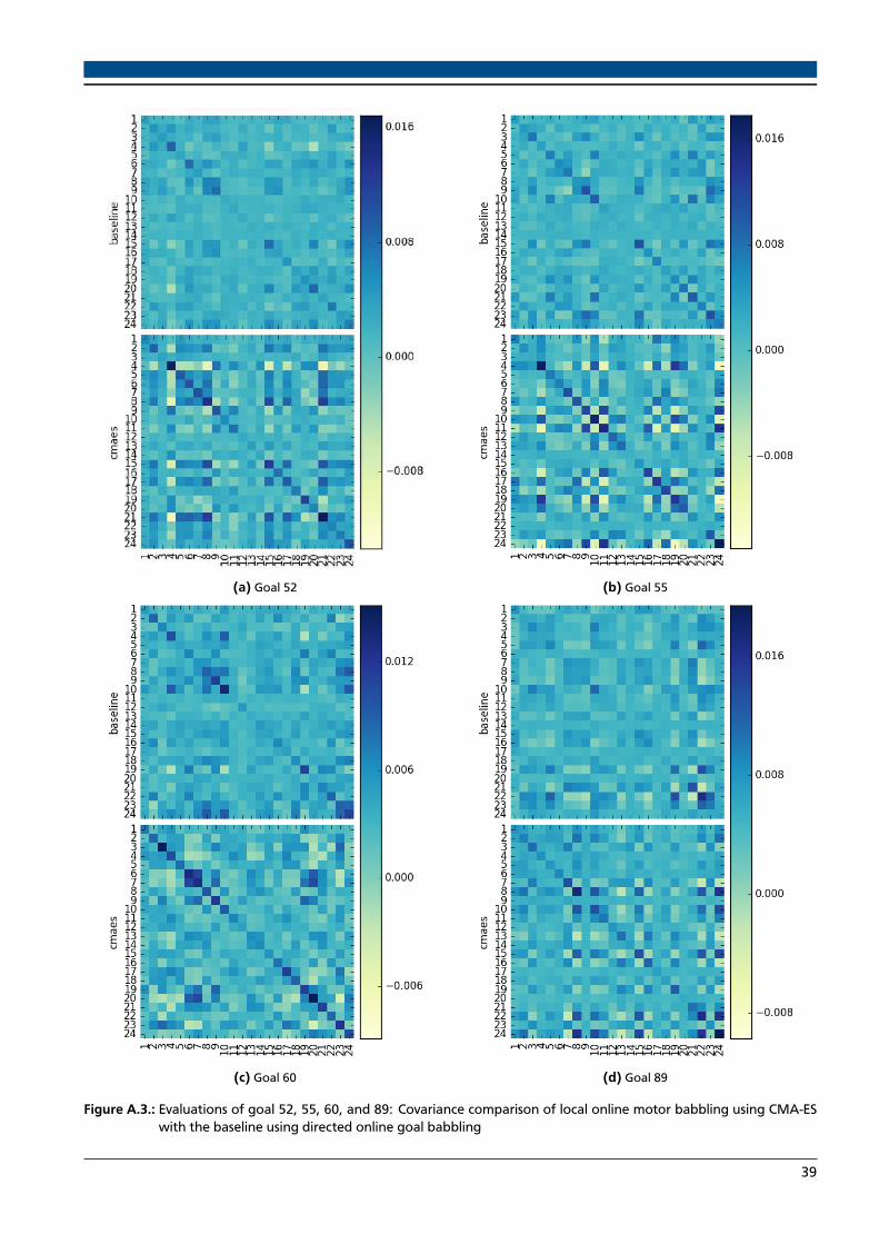
(a) Goal 52 (b) Goal 55

(c) Goal 60 (d) Goal 89

Figure A.3.: Evaluations of goal 52, 55, 60, and 89: Covariance comparison of local online motor babbling using CMA-ESwith the baseline using directed online goal babbling

39