Embed Size (px)
Citation preview

Local Microcode Compact ion Techniques
DAVID LANDSKOV, SCOTT DAVIDSON, AND BRUCE SHRIVER University of Southwestern Louisiana, Computer Science Department, P.O. Box 44330 U.S.L., Lafayette, Louisiana 70504
PATRICK W. MALLETT Computer Sciences Corporation, 6565 Arlington Boulevard, Falls Church, Virginia 22046
Microcode compaction is an essential tool for the compilation of high-level language microprograms into microinstructions with parallel microoperations. Although guaranteeing minimum execution time is an exponentially complex problem, recent research indicates that it is not difficult to obtain practical results. This paper, which assumes no prior knowledge of microprogramming on the part of the reader, surveys the approaches that have been developed for compacting microcode. A comprehensive terminology for the area is presented, as well as a general model of processor behavior suitable for comparing the algorithms. Execution examples and a discussion of strengths and weaknesses are given for each of the four classes of loc .al compaction algorithms: linear, critical path, branch and bound, and list scheduling. Local compaction, which applies to jump-free code, is fundamental to any compaction technique. The presentation emphasizes the conceptual distinction between data dependency and conflict analysis.
Keywords and Phrases: compaction, data dependency, horizontal architecture, horizontal optimization, microcode compaction, microinstruction, microprogram, parallel, resource conflict, scheduling
CR Categories: 4.12, 6.21, 6.33
INTRODUCTION
As the use of microprogramming increases, it becomes costly to write microprograms in unstructured unwieldy languages. The same pressures that led to the widespread acceptance of conventional high-level lan- guages now apply to microprogramming [DAvI78]. The time is long overdue for the development of machine-independent, high-level microprogramming language compilers.
This work was supported in part by the National Science Foundation under Grant MCS 76-01661.
Microprogrammable processors that al- low simultaneous control of several hard- ware resources present special challenges to the implementor of a high-level language compiler. These horizontal processors must have their microprograms compacted in or- der to run efficiently. Compaction involves choosing from the possible arrangements of concurrent activities one that will minimize the execution time of the microprogram and possibly its size as well.
The first step in such a compaction is the division of the program into branch-free segments. The analysis, or local compac- tion, of one of these segments is an expo-
Permission to copy without fee all or part of this material is granted provided that the copies are not made or distributed for direct commercial advantage, the ACM copyright notice and the title of the publication and its date appear, and notice is given that copying is by permission of the Association for Computing Machinery. To copy otherwise, or to republish, requires a fee and/or specific permission. © 1980 ACM 0010-4892/80/0900-0261 $00.75
Computing Surveys, Vol. 12, No. 3, September 1980

262
CONTENTS
• D. Landskov, S. Davidson, B. Shriver, P. W. Mallett
INTRODUCTION DefinitiQn of the Problem The Minimum Manhole Shifts Analogy How This Paper Is Organized
1. DATA DEPENDENCY ANALYSIS 1.1 The Definition of Data Dependency 1.2 Extending the Data Dependency Concept 1.3 Forming a Data Dependency Graph
2. DESCRIBING THE HOST MACHINE 2.1 Micmoperation Tuples 2.2 Rehtionships Between Tuples
3. FORMING COMPLETE INSTRUCTIONS 3.1 Tile FormCIs Algorithm 3,2 Alternative Approaches
4. COMPACTION ALGORI~4MS 4.1 The Linear, Algorithm
• 4.2 The Critical Pafit Algorithm 4.3 The Branch and Bound Algorithm 4.4 Branch and Bound Heuristics and List Sched-
unng 4.5 Computational Complexity 4.6 Register Allocation
5. CONCLUSIONS GLOSSARY ACKNOWLEDGMENTS REFERENCES
T
nentially complex problem, i.e., one that is time consuming to calculate. In the past, because of this complexity, it was feared that a compiler capable of generating effi- cient horizontal microcode would run too slowly to be. usable. Because micropro- grams are at the lowest programmable level, their efficiency directly affects the efficiency of the entire system.
Recent research [TOKo77, MALL78, WOOD79, FXSH79] indicates that local com- paction algorithms can be practical. De- spite the theoretical computational com- plexity, optima[ or near-optimal results can be found in a reasonable (i.e., nonexponen- tial) amount of time. Thus one of the major obstacles to practical microcode compilers for horizontal machines is surmountable.
This paper surveys the various ap- proaches that have been taken for com- pacting microcode [RAMA74, TABA74, TSUC74, YAU74, DEWx75, AGER76, DASG76, MALL78, WOOD78, FISH79] . Clear defini- tions are presented for the terms required
to understand this area, since the variations in terminology and the lack of a compre- hensive vocabulary have constituted a ma- jor problem. This paper presents a unifying terminology for studying the issues in- volved and applies this terminology to the different approaches.
The development of compaction algo- rithms in existing literature is based on a number of different models of the processor environment. These differences make com- parison of the algorithms difficult, and sometimes model differences are confused with the differences in the algorithms them- selves. This paper presents a model which incorporates the major features of existing models, yet avoids unnecessary details. All of the algorithms presented are explained in terms of this general model.
Local compaction is a fundamental part of any compaction process. There are four major classes of algorithms for locally com- pacting microcode: linear analysis, critical path, branch and bound, and list schedul- ing. Each of these classes is explained using the terms defined in this paper. A common example illustrates the execution of each kind of algorithm. There are also detailed presentations of two nontrivial support al- gorithms which are rarely explained in the literature.
Definition of the Problem
A microprogram is a sequence of microin- s t ruc t ions (MIs). A microprogram is stored in a memory, often a special memory called the control store, from which the instructions are executed one at a time. During its execution, an MI is the control .word for its machine.
Each separate machine activity specified in an MI is called a m i c r o o p e r a t i o n (MO). Thus an MI can be characterized as a set of MOs. A field is a collection of control word bits that controls a primitive machine ac- tivity. An MO requires one or more fields in order to execute. The format of a control word determines how many and which MOs can be placed together in an MI. Figure 1 shows the relationship between fields and microoperations in the control word orga- nization for a hypothetical machine. If only
~one or a few MOs can fit into an MI, the
Computing Surveys, Vol. 12. N 0. 3, September 1980

Fieldl
Local Microcode Compaction Techniques
Source Destination Field2 Field Field
263
(a)
Field1 Field2 Source Destination
rno~: ADD d too2: MOVE s mo3: SHIFTL n mo4: SHIFTR n
where s, d E AC (accumulator), RA (reg A), RB, or SH (shifter); n ~ I. ,4. (b)
MOVE empty
I ISHIFTL 13R I (c)
FIGURE 1. Example control word organization. (a) Microinstruction format. (b) Partial list of microop- erations. (c) Two possible microinstructions.
machine is said to have a ver t ica l archi- tecture. Otherwise it is said to have a hor izonta l a rch i tec ture . A more detailed discussion of control word format can be found in DASG79.
The microcode c o m p a c t i o n p r o b l e m is as follows. Suppose that for a particular machine, the hos t machine , we are given a microprogram expressed as a sequence of MOs. These MOs are to be placed into MIs so that the microprogram execution time is minimized. This must be done under the restriction that the resulting sequence of MIs must be semantically equivalent to the original sequence of MOs. "Semantically equivalent" means that if both sequences are executed, the same input always results in the same output. The original sequence of MOs is not executable as it stands but can easily be made executable by placing each MO in a separate MI. Some MOs may have to be placed in the same MI as a previous MO, as explained in the section on coupling. Informally, the problem is to
"compact" the program into a small mem- ory space.
We discuss microcode compaction for horizontal architectures. Although compac- tion can be performed for any architecture, including a vertical one, the compaction problem is only interesting if a useful con- currency of MO execution can be achieved. Not only are vertical architectures limited in their potential concurrency, but this lim- itation is one of the justifications of their design. Vertical machines are easier to mi- croprogram precisely because they avoid the time-consuming and error-prone pro- cedure of manually analyzing concurrency.
In order to analyze possible concurrent activity, the microprogram is divided into straight-line microcode sections.
Definition. A straight-Hne microcode sec t ion (ELM) is an ordered collection of MOs with no entry points, except at the beginning, and no branches, except possibly at the end.
Computing Surveys, Vol. 12, No. 3, September 1980

264 • D. Landskov, S. Davidson, B. Shriver, P. W. Mallett
HLL i '" microprogram
Compile to MO level
G e n e r a t e MOs
Apply conventional code optimization
List of MOs
Host MO Definition
Table
Analyze flow of control
SLMs i !
(Locally) compact each SLM
List of Mls
IZIOgl~ "2, One poa~)le microcode compilation system.
SLMs are also known as basic blocks. Within ~ SLM, minimizing execution time is achieved by minimizing the number of compacted microinstructions. Analysis of a single SLM is called local analysis , and of more than one SLM, global analysis.
In global analysis, minimizing the num- ber of microinstrUctions does not necessar- ily minimize execution time, since some SLMs may be executed many more times
than others. Global analysis is very much an active research problem [TOKo78, DAso79, WooD79, FzSH79]. Interesting ap- proaches based on treating a compacted SLM as a primitive in a more global SLM are found in WOOD79 and FISH79. Our pa- per is confined to the local analysis prob- lem, which is examined in detail.
The role of local compaction analysis in a high-leval microprogramming language
C o m p u ~ Surve:~J, Vol. 1~ NO. 3, September 1980

Local Microcode Compaction Techniques • 265
, I COMPACT EACH SLM I
FI(}URE 3. Subalgorithm modules BuildDDG and FormCIs are used
translation system [cf. MALL75] is shown in Figure 2. Two relatively distinct analyses must be performed as part of the local compaction process (see Figure 3). The way in which data are passed from MO to MO forces some MOs to be kept in the order in which they appeared in the original SLM. Data dependency ana lys i s decides the partial ordering. Confl ict ana lys i s deter- mines whether two MOs can fit into the same MI without conflicting over a hard- ware resource.
Many of the optimization techniques of conventional compilers are applicable to microprograms--which is not surprising, since a sequence of MOs strongly resembles a conventional machine language program [KLEI71]. These techniques consist primar- ily of code transformations that reduce the number or the execution time of MOs in sequential form. For the rest of our discus- sion we assume that any code transforma- tions have already been applied.
Sometimes compaction is termed hori- zontal optimization, but this is misleading because conventional compiler optimiza- tion is different from compaction and be- cause compaction can reduce micropro- gram size and execution time without nec- essarily minimizing them. Horizontal im- provement would be a more accurate term.
The Minimum Manhole Shifts Analogy
The reader can gain an appreciation for some of the issues involved by considering the following analogy, in which the sched- uling problems of an underground con~struc- tion project are compared to those of local
Data Dependency Analysis
(BuildDDG) i
Conflict Analysis
(FormCls)
used by compaction algorithms. in most of the approaches.
microcode compaction. The appropriate compaction term is placed in parentheses following discussion in the applicable anal. ogy.
Both compaction and this analogy are examples of job shop scheduling problems [COFF76]. Compaction also bears a direct resemblance to the processor scheduling problem [GoNz77].
The Analogy
The foreman of a crew working in a man- hole has a big job to do. The job entails a large number of specific tasks, but there is no shortage of workers. There is, however, a limited amount of space in the manhole and a limited number of tools. The fore- man's problem is how to perform a given job in the minimum number of shifts.
The analogy thus far:
The manhole: an MI or a control store word.
The shift: one MI cycle. The job: an SLM. The task and its associated worker: an MO. The tool: a processor's operational unit
(ALU, BUS, etc.)
Some workers' tasks depend on the com- pletion of tasks by other workers. The foreman must make a list of which tasks depend on which other tasks and not send a worker down into the manhole before the necessary prerequisite tasks have been completed (data dependency).
Assume for now that a worker's task al- ways takes exactly one shift to complete (monophase MI). Thus a worker depend-
Computing Surveys, VoL 12, No. 3, September 1980

266 , D. Landskov, S. Davidson, B. Shriver, P. W. Mailett
ing o n the job done by another should not go into the manhole until the shift ~ r that of the first worker. Of course, the tasks of twoworke r s do not~always involve a dependency. I f this is the case, they can go down into the manhole together, assuming there are no other problems between them (data independence).
When can workers with independent tasks not be sent down into the manhole together? There are two possibilities. First, they may require the same tool to do their jobs. If there is only one such tool, one worker must wait for the next shift (re- source unit conflict). Second, the two work- ers may not fit into the manhole together. This can happen if the two workers must work in the same place (at an exposed water pipe, for instance) in the manhole (mi- crooperation field conflict).
Now, w h a t i f the assumption that each worker needs an entire shift is unrealistic? Suppose that some workers need only part of a shift to perform their .t~ks (polyphase MIs). A union rule states that a worker must stay in the manhole during the entire eight-hour shift, but also that a worker may be idle some of that time. Consider two workers with independent tasks who need the same tool.• I f they can work at separate times, one can use the tool for the first few hours, the other, for the remaining :hours. Thus two workers who need the same tool during different par t s of the shift can be sent into the manhole together (resource unit compatibility). They still must fit to- gether in the manhole, however (mieroop- eration field compatibility).
Suppose worker 2's task can only be per- formed after the completion of worker l 's task. If worker 1 starts in the morning and takes two hours to finish and worker 2 needs four hours, they can be sent into the manhole together, worker 2 waiting until worker 1 is finished. Thus, assuming that the workers can fit together in the manhole, they can~ be sent down together (weakly dependent MOs):
Now, let worker 3 perform a delicate task, such as cleaning a joint in preparation for welding. Worker 4 does the welding. If the cleaned joint is left overnight, it gets dirty again, and the job must be redone. There- fore worker 4 must be sent into the manhole
on the same shift as worker 3 (coupled MOs). The foreman decides to simplify the analysis of task dependencies by consider- ing two or more inseparable tasks as one task with multiple workers (Me bundles).
Some tools may be multifunctional. A drill can be used for drilling or modified and used for polishing, but a polisher can be used only for polishing. If worker 5 needs a drill and worker 6 a polisher, worker 6 should be given the polisher, not the drill/ polisher. The foreman should tell the work- ers which tools to use, thus eliminating this kind of conflict (versions of resource units). Similarly, ff worker 7 can work either in a corner or by a wall (needing access to pipes, say), and worker 8 can work only on a junction box in a corner, worker 7 should be told to work by a wall (versions of mi- crooperation fields).
These are some of the issues the foreman must contend with when attempting to minimize the number of shifts required to complete a job.
The manhole analogy makes the sched- uling nature of the local compaction prob- lem clear. The terms in parentheses are explained in the appropriate sections of this paper. The reader should refer to this anal- ogy when studying these terms.
How This Paper Is Organized
Many of the sections in this paper are ex- planations of algorithms. Although the de- tails of an algorithm can be skipped without a serious loss of understanding of subse- quent sections, it is crucial to understand the problem that each algorithm is designed to solve.
Section 1 analyzes the data dependency problem and presents an algorithm for building a data dependency graph from an SLM in sequential form. Section 2 explains a model of processor behavior and shows how it can be used to detect conflicts in resource usage. Section 3 examines an al- gorithm that uses this model to form mi- croinstructions. Finally, Section 4 presents examples from each of the four classes of compaction algorithms and discusses the computational complexity of each class.
Little or no prior knowledge of micropro-
Computing SurVeys, Vol.12, No. 3, Sei~ember 1980
• i :

L o c a l M i c r o c o d e C o m p a c t i o n T e c h n i q u e s , 267
gramming is needed in order to understand this article.
1. DATA DEPENDENCY ANALYSIS
Data dependency analysis is the first step performed in the local compaction process. It is based on an examination of the input and output resources of each microopera- tion.
1.1 The Definition of Data Dependency
Most of the microoperations of a given ma- chine operate on registers . A register whose value is used by an MO is called an inpu t storage resource or an input operand. Similarly, a register whose value is changed by an MO is called an ou tpu t storage re- source or an output operand. ("Source" is often used instead of "input" and "sink" or "destination" instead of "output.")
As long as the number of variables used in the entire microprogram (not just one SLM) does not exceed the number of reg- isters available, a register is essentially a variable. Assume for now that this is the case; the problem of reallocating registers is discussed in Section 4.6.
Given an SLM to be compacted, the final list of MIs must be "semantically equiva- lent" to the SLM in the sense that both must produce the same results when given the same input values. If they are not se- mantically equivalent, data integrity has been violated. Some of the MOs cannot change their order of execution without producing different answers. In particular, the order of two MOs cannot be changed if they satisfy the following definition.
Def in i t ion . Two MOs, moi and moj, have a data interact ion if they satisfy any of the following conditions (assuming that moi precedes moj in the original SLM):
(1) An output resource of moi is also an input resource of moj (if moj were first, it would have an old value in its input resource, one that should have been updated by moi but was not).
(2) An input resource of moi is also an output resource of moj (if moj were first, it would be able to change the value that moi was expecting as input before moi had a chance to use it).
(3) An output resource of moi is also an output resource of moj (if moy were first, moi would be able to overwrite moj 's output value, when m o f s value is the one that should remain after both MOs are finished).
The definition of data interaction can be applied to any two MOs without reference to their order in the original SLM. Section 2 presents a representation for the input and output resources of MOs that allows data interaction to be tested by examining set intersections.
The remainder of our development of data dependency analysis rests on the fol- lowing assertion.
A compacted list of MIs will be semanti- cally equivalent to its original SLM if, for every two MOs in the MI list that have a data interaction, the MO occurring ear- lier in the SLM finishes with each of the resources causing the data interaction be- fore the later MO starts to use it.
Several definitions are based on this as- sertion, as shown in the following.
Def in i t ion . Given two MOs, moi and moj, where moi precedes moj in the SLM, then these MOs are o rde r p re se rv ing if their execution in the same MI obeys the following rule (assume it is otherwise pos- sible): For each resource causing a data interaction between them, moi finishes with that resource before moj starts to use it.
If two MOs are order preserving, they can be in the same MI without violating data integrity. If an MO is order preserving with respect to every MO in an MI, it is order preserving with respect to that MI.
The next definition defines a partial or- der over the MOs.
Def in i t ion . Given two MOs, moi and moj, where moi precedes moj in the original SLM, moj is d i rec t ly d a t a dependen t on moi {written moi ddd moj) if the two MOs have a data interaction and if there is no sequence of MOs, mokl, rook2 . . . . , mok , , n -- 1, such that moi ddd mokl, mokl ddd r o O k 2 . . . . . roOk(n-l) ddd mokn, mOkn ddd moj.
The second part of the definition ensures that two directly data-dependent MOs will
Computing Surwyo, Vol. 12, I ~ 3, September 1980

268
have no "chain" of directly data-dependent MOs between them.
Data dependency is the transitive closure of the direct data dependency relation.
Definition. Given two MOs, moi and moi, mo~ is data dependent on mo~ (writ- t e n mo~ dd moj) if
moi ddd mo#
or if there exists an Me , rook, such that
moi ddd rook and rook dd moj.
If mo~ dd moj, then moj cannot execute before moi without violating data integrity. Usually they cannot execute in the same MI either; this situation is discussed in the next section. Two MOs that are not data dependent are said to be d a t a indepen- dent . It should be clear that data indepen- dence implies order preservation.
Suppose a list of MIs is being constructed from an SLM and the MOs in the SLM are being considered one at a time. The data dependency concept is used to determine whether adding a particular M e to a par- ticular MI in the list will violate data integ- rity. If the answer is no, the M e is said to be d a t a ava i lab le with respect to that MI. Data availability is discussed more formally in the next section.
The direct data dependency relation de- fines a partial order over the MOs of an SLM. The representation of this ordering in graph form is called a d a t a dependency g r a p h (DDG). Each node on a DDG, node i say, corresponds to a unique MO in the SLM, moi. If there is a link from i to j on the graph, then mo~ ddd moj. The definition of direct data dependency ensures that this link is the only path in the graph from i to j. Figure 4 shows a simple DDG where mol
• D. Landskov , S. Davidson, B. Shriver, P. W. Mal l e t t
(1) /
(2)
(3) FIOUBE 4. A data dependency graph. Nodes I and 3 cannot be linked.
ddd mo2 and mo2 ddd too3. There cannot be a link between node 1 and node 3 be- cause they are already linked indirectly.
Many compaction algorithms use a DDG of the SLM as input (see Section 4). A well- designed microcode compilation system might have the code generator produce the MOs in graph form. Otherwise, the first step of compaction is to form a DDG from the SLM.
1.2 Extending the Data Dependency Concept
There are several machine features that can be incorporated into data dependency analysis.
1.2.1 Finishing with a Resource Before the End of a Cycle
Sometimes an M e does not affect machine resources during the entire time that the machine allows an MI to execute (i.e., the instruction cycle time). In Section 2, a no- tation for specifying the parts of an MI cycle in which an M e executes is devel- oped. If mo~ and moi are in the same MI, and if moi finishes executing before moj begins, then data integrity is preserved even i f me# is data dependent on moi. This mo- tivates the following definition.
Definit ion. Given two MOs, moi and moj, then moj is w e a k l y d e p e n d e n t on moi (moi w d moj) i f moj is directly data depen- dent on moi, and if for every resource caus- ing a data interaction between them, moi finishes with that resource before me~ starts to use it.
Clearly, taking advantage of weak de- pendencies makes compactions with fewer MIs possible, since two MOs related by a weak dependency may be able to fit into the same MI. In DASO76, the term "condi- tionally disjoint" is almost a synonym for weakly dependent (the difference in mean- ing arises from model differences and is not significant). If moi ddd moj, and it is known that moi is not weakly dependent on mo~, then moi is strongly dependent on mo~ (moi sd moy). If MOs are placed in a list of MIs so that the MOs are order preserving,
mo~ sd moj implies mo~ < moj mo~ wd moj implies mo~ <_ me~
The weak dependency concept allows a more precise analysis of some of the M e
Computing Surveys, Vol. 12, I'4o. 3, September L980

Local Microcode Compaction Techniques • 269
relationships. One conclusion that can be drawn is
If two MOs are data independent, or if one is weakly dependent on the other, then they are order preserving.
These are the only two conditions consid- ered here which allow two MOs to fit into the same MI and still preserve data integ- rity.
The term d a t a avai lable applies when a list of MIs is considered instead of just an individual MI. We observe that
Given an SLM of MOs, and a list of MIs constructed from some of these MOs, moi is called data available with respect to mij if
(1) every MO in the SLM on which moi is data dependent appears in an MI which is above mij in the list, or ap- pears in mij itself, and
(2) moi is not strongly dependent on any MO in mij.
Item 2 is a rewording of order preservation. Notice that this definition applies even if mi~ is empty, or if the list of MIs has no other elements.
•.2.2 Transitory-Data Resources
One particular kind of weak dependency has a special importance. The example in Figure 5 depicts an MI sequence in which mol, too2, and mo3 combine to take the data stored in register A1 and move (gate) it through latches 1 and 2 to register A2.
Registers A1 and A2 are examples of s ta t ic resources. A static storage resource is one whose contents are maintained in- definitely until explicitly overwritten by the execution of an MO. A transitory-data storage resource is any storage resource that is not static, that is, one whose con- tents can become undefined at the termi- nation of an MI in which it has been given a value. Latches are examples of transitory- data resources.
Two MOs are said to be d i rec t ly cou- pled if one of them passes data to the other through a transitory-data resource. Two MOs are said to be coupled if a sequence of MOs exists such that one of the two MOs
mo~: Input ffi A1, Output - Latchl i (MOs activating devices that use
the contents of Latch1) mo2". Input ffi Latch1, Output ~ Latch2
: (MOs activating devices that use the contents of Latch 2)
mo3: Input ffi Latch2, Output ffi A2
FIGURE 5. MOs coupled through transitory-data resources.
is the first element of the sequence, the other is _the last, and each element of the sequence is directly coupled to its adjacent elements. Coupled MOs must be placed in the same MI to work properly. Coupling can occur in a variety of microprogram instruction sets [AGRA76, SHRI73].
It is the authors' experience that the only way to accommodate coupling in the com- paction algorithms without causing serious confusion is to incorporate coupling into the definitions of the MO-to-M0 relation- ships. This can be done using the concept of bundling.
Definition. A mic roope ra t ion bund le (MB) is a set of MOs, all of which are coupled to one another.
Thus every MO in an MB must go into the same MI because of the nature of tran- sitory-data resources.
The SLM is changed from a list of MOs to a list of MBs by putting coupled MOs into the same MB and by putting each uncoupled MO into its own MB. All of the relations over MOs can be defined over MBs in a straightforward manner. For ex- ample, mbj is data dependent on mbi (mbi dd mbj) if there exists an moi in mbi and an moj in mbj such that moi dd moj.
After the MB relationships are defined, the compaction algorithms can operate with MBs just as they previously operated with MOs. The nodes of a D D G are now MBs, and compaction algorithms change an SLM of MBs into a list of MIs. An MI is now a set of MBs.
For the rest of this paper we discuss compaction in terms of MBs. When relating this paper to other papers that do not dis- cuss coupling, the reader may substitute the word microoperation for microopera- tion bundle.
Computing Surveys, Voi. 12, No. 3, September 1980

270
1.2.3 Multicycle Operations
In many mach ines there are microopera- tions which need more than one instruction cycle to exJ~cute. Amain memory reference is a common example of such a multicyc!e operation. An MB which is data dependent on an MB containing a multicycle operation must be d e l a y e d the proper number of cycles following the multicycle MI's start- up. This is easily accomplished in data de- pendency analysis by using d u m m y mi- crooperation bundles . An operation re- quiring n cycles to execute is represented by a sequence of n MBs, each one data dependent on the previous MB in the se- quence. The first MB has all Of the input and output resources of the operation; the others are dummies which use the delayed output resources of the operation for both input and output. Figure 6 shows an ex- ample DDG where mbl has a three-cycle operation. Nodes la and lb represent dummy MBs.
(1) I
( l a ) ( 2 ) I "
k ( l b ) I
( 3 )
FIGURe. 6. A data dependency graph with a three-cycle mi- crooperation.
• D. Landskov, S. Davidson, B. Shriver, P. W. Mallett
Although dummy MBs do not corre- spond to actual microoperations, an MI containing only dummy MBs has to be created as a no-operation (NOOP). Such a NOOP indicates that the machine has noth- ing else to do while waiting for the comple- tion of a multicycle operation. Global anal- ysis can eliminate NOOPs at the end of an SLM by moving the corresponding dummy MBs to all the SLMs that can execute immediately after this one [MALL78].
1.3 Forming a Data Dependency Graph
Few of the compaction articles referenced by this paper define an algorithm for con- structing a data dependency graph from a list of MBs (or MOs). Although algorithms of this kind exist, they are not widely known and have not been explained in terms of the
mi'crocode compaction problem. Thus the following algorithm should be of general interest.
The algori thm presented (BuildDDG) cor~structs t h e g r a p h o n e MB at a time, starting with the first MB in the list and proceeding through the list in sequential order. Each MB is added as a new node to the graph formed by the MB's predecessors in the list. Then the graph is searched to find which nodes should be linked to this new node. We say that we are adding the "current MB" to the "current graph."
The directed graph is defined in a con- ventional way. "Node A is a parent of node B" means that "B is directly data depen- dent on A"; we write node A above node B with a link, or line, connecting them. The nodes without parents are the roots , and are drawn at the top of the graph. The nodes with no children are the leaves . A path is a sequence of distinct nodes, each of which is a parent to the next node in the sequence. Node A is an a n c e s t o r of node B if a path exists from A to B.
While adding the current MB to the graph, we test an MB already in the graph (a graph MB) to see if the current MB is data dependent on it. Whenever the test indicates a data dependency, a link is formed. Each graph MB needs to be tested once at most when adding the current MB. The data interaction part of the test can be performed by looking at only the two MBs involved. However the definition of direct data dependency tells us when data inter- action does not imply direct data depend- ency. We can restate this part of the defi- nition as follows:
If the cu r r en t microoperation bundle, mbk, is directly data dependent on a mi- crooperation bundle, mbj, then mbk can- not bed i r ec t l y data dependent on an ancestor of mbi.
It immediately follows that a graph-MB should not be linked if it is an ancestor of the current MB. Such links are not formed, and the unnecessary testing of such MBs for data interaction is avoided by observing the following rule:
Data lnteraction Testing Rule. A graph MB is tested for data interaction with the current MB if and only if all of the graph
Computing Surv~s, Vol. 12, No. 3, September 1080

Direct Data Dependencies:
Current Current Compare Graph MB to
(1) /
(2)
(I) (3) /
(2)
(I) (3) / \
(2) (4)
(I) (3) / \
(2) (4) I
(5)
w
2 I
4
2 I
3
2
4
3
2
Local Microcode Compaction Techn~ues
i i l l i
I ddd 2, I ddd 6, 4 ddd 5. I ddd 4, 3 ddd 6,
i
t~ext ddd? Action
no
no
no yes
no
no
yes
no
no
5 no 4 no
I yes
3 yes
Add node for 3; Test next leaf (2).
Check 2's parents. (No parent); Next MB.
Add node for 4; Test next leaf (2).
Check 2's parents. Form link from I to 4;
Test next leaf (3). (No parent); Next MB.
Add node for 5; Test next leaf (2).
(2's parent has untested child, 4); Test next leaf (4).
Form link from 4 to 5; Test next leaf (3).
(No parent); t~ext MB.
Add node for 6; Test next leaf (2).
(2's parent has untested child, 4); Test next leaf (5).
Check 5's parents. Check 4's parents (1's
children now verified) Form link from I to 6;
Test next leaf (3). Form link from 3 to 6;
Stop (out of gBs).
271
(I) (3)
/ 1 \ / (2) (4) (5)
I (5)
Resulting Data Dependency Graph
FIGURE 7. Example of formation of a data dependency graph.
MB's children are verified nonancestors of the current MB.
By following this rule a positive test for data interaction implies direct data depend- ency.
Now an algorithm that searches for graph nodes on which the current MB is directly data dependent can be specified. A search
progresses upward from each leaf, since each leaf automatically satisfies the testing rule. If the test of an MB for data interac- tion is positive, then a link is formed to the current MB. If the test is negative, then that MB has been verified as a nonancestor of the current MB. Each of its parents is informed that another child has been veri-
Computing Surveys, Vol. 12, No. 3, September 1980

272 • D . Landskov, S. Davidson, B. Shriver, P. W. Mallett
fled. Each parent is also checked to see if it now satisfies the testing rule. If it does, then the parent is tested..Searching ends when there are no more MBs to be tested.
Figure 7 shows the formation of a data dependency graph from an SLM of six MBs. The direct data dependencies which should be detected by the algorithm are listed at the top of the illustration. The algorithm starts by placing mbl in the graph. Then mb2 becomes the current MB. Since mbl is a leaf of the current graph, it is tested against mb2 for data interaction. The test is positive and a link is formed. No more MBs remain to be tested, so mb~ becomes the new current MB. Refer to Figure 7 for a trace of the rest of the exe- cution.
The resulting data dependency graph shows that it is not possible for mb5 to be directly data dependent on mb~ (since they are indirectly linked on the graph), even though there may be a data interaction between them. The algorithm did not per- form the needless test for this data inter- action. Notice also that the algorithm searches parents (and leaves) from left to right. The order in which parents are searched makes no difference. The searches could proceed in parallel.
No reference has been made yet to the data structure used to represent the graph. Any structure capable of representing a directed graph will work. An adjacency ma- trix where DDG~ -= true means mbi ddd mb~ is a reasonable choice.
2. DESCRIBING THE HOST MACHINE
Section I examined the ordering that must be preserved while placing microoperation bundles into microinstructions. There re- mains the question of the restrictions im- posed by the host machine itself. Two MBs cannot be placed in the same MI if they both need exclusive control over the same
• resource at the same time. Such a situation is called a conflict. For example, usually two MBs cannot use the same ALU at the same time.
To be able to detect conflicts, a compac- tion algorithm must operate within the framework of a machine model. More pre- cisely, this framework should be a model of a machine control word, since control word
Comp,t~S,rvey~VoLla, No.a, S e l ~ " 19S0
behavior defines the legality of an MI. This model should have the following properties.
Machine independence. The model should be applicable to a variety of physical machineL Table-driven models can isolate machine-dependent information, such as the host instruction set or the number of resources of a given type. In any case the data structures used by the compaction algorithms should be general.
Manageability.The data structures used by the model should support clear, well. structured design. Appropriate primitives should be defined and used in the code. The model should not contain hardware details unnecessary for the execution of the algo- rithms. Efficiency should also be consid- ered, since some potential uses of the model involve computations of exponential com- plexity.
Completeness. The model must be able to represent real-world machines. This im- plies that some machine features ignored in the past will have to be supported by the model. Designing a simple model and add- ing extensions later can have disastrous effects on its manageability.
In the following sections we present a model which is a synthesis of most of the models in the literature [I~EI74, DAsQ76, DEW176, MALL78, RAMA74, YAU74]. This model demonstrates that the above goals can be (and have been) met. Several fea- tures of this model contribute to its com- pleteness. One previously mentioned is the ability to represent microoperatious that are not active throughout an entire MI cycle. A machine that supports such MOs is said to have polyphase timing. Many compaction algorithms deal only with monophase timing [DEWI76, RAMA74, YAU74]. Another important feature of the model we are presenting is the ability to delay resource binding until MIs are formed, that is, until the compaction pro- cess. Some models do this for registers only [DEWI76]. The binding concept allows an MO to have a choice of other kinds of resources as well.
This model is not claimed to be the best choice for all compaction problems but is offered to demonstrate the feasibility of describing a variety of realistic machine features. Although coding details are not

Local Microcode Compaction Tedb-dques • 273
m__oo[i] : <ADD, {A, B}, Latchl, ADDERI, Phase2, Field1>
explanation: Latchl <- A + B; Adder ADDERI is used to add the contents of its two input registers A and B. The results are placed in the register Latchl. Execution occurs during clock phase 2. The encoding for the MO is contained in MO field Fieldl. The name of the MO is "ADD."
m_~o[j] : <MOVE, A, B, BUS, PhaseO, Field2>
explanation: B <- A; Using the bus BUS, data is gated from register A to B. Execution is at clock phase PhaseO and the MO's encoding is in MO field Field2.
mo[k] : <JUMP, empty, empty, CSAU, PhaseS, {Field5, Field6:"9"}>
explanation: Unconditional Branch; The Control Store Address Unit (CSAU) uses the immediate data (9) contained in MO field Field6 as the target address for the branch. Execution occurs at Phase5, and Field5 contains the encoding of the MO. Ho input or output resources are required.
i
m~o[l] = <SHIFT, ShiftA, ShiftA, SHIFTER, Phase3, Field3>
explanation: ShiftA <- SHIFTER(ShiftA); The shifter SHIFTER is used to shift the contents of register ShiftA. Execution is during clock phase Phase3. The encoding occupies MO field Field3.
FIGURE 8. Examples of MO tuple representation.
presented here, implementations of the fea- tures do exist [MALL78, WOOD78, FISH79].
2.1 Microoperation Tuples
The MO is the most primitive activity ac- commodated in our model. An MB is rep- resented as a set of MOs. The semantics of an MO are represented by a six-tuple, (name, I, O, U, T, F), where the tuple elements are
(1) name--an identification of the MO to be performed,
(2) I - - the set of all storage resources whose contents are required by the MO as input,
(3) O-- the set of all storage resources into which the MO places output,
(4) U-- the set of all functional units re-
quired by the MO while the MO is executing,
(5) T- - the set of processor clock phases required for MO execution, and
(6) F-- the set of all microinstruction fields required by the MO (they contain the encoding of the MO and possibly im- mediate data).
Elements 2 through 6 are known as tuple sets. Figure 8 shows examples of four MOs with their tuple sets enumerated. Note that the "{" and "}" braces are not written around singleton sets. An MI is a group of MOs contained in one word of control store. The execution time for one MI is called the instruction cycle t ime and may consist of several subcycles cal led clock phases. A microprogram is an ordered list of MOs or

274 • D. Landskov, S. Davidson, B. Shriver, P. W. Mallett
MIs which real i~ the logic of a particular " ular binding upon all Orlists within a tuple
The six-tuple specification of M0 sen;an- tics is a machine-independent representa- tion o f a mic/ooperation: When t h e MO s and resources of a particular machine are enumerated in this format, the representa- tion becomes tailored to that machine. The tuple is used by a code compaction algo- rithm to detect conflicts and analyze re- source usage between MOs.
The definition of the individual sets of the six-tuple, as given in Figure 8, is not complete. We extend it to take into account r e s o u r c e al locat ion. The tuple se ts are considered to be b o u n d or u n b o u n d with respect to their allocated processor re- sources. An unbound set contains, as ele- ments, the enumeration of all possible re- sources that can be allocated to the set. A bound set contains, as elements, those re- sources that were actually assigned to the set. Consider the following unbound Unit set (Uset).
Ui ffi (ALU1 or ALU2}
This set is characterized as unbound by its "or" operator, which indicates an Orlist . The Orlist signifies that at some point be- fore the MO can be executed, achoios must be made as to which hardware resource will be assigned to beused by the MO. An Orlist in which the assignments have been made (i.e., the Orlist has only one item in the list) is a v e r s i o n o f the set. For example, bind- ing the foregoing User generates two bound Orlists and thus two versions of the Uset:
U ~ e r l = {ALUI) U ~ e r 2 = (ALU2)
Another resource allocation grouping is the Andlist , which groups one or more Orlists in an unbound or bound tuple set. Consider an example o f an unbound Uset:
U j = ((ALU1 or ALU2), (ALU3 or ALU4))
The Andlist indicates that one unit must be assigned from each Orlist. One version of Uj is
: UjVer l ffi (ALU1, ALU3)
Tuple sets are either bound or unbound sets. Resource allocation imposes a partic-
The elements of a field set (Fset) specify the MI fields used for storage of the encod- ings of the MOs and immediate (literal) data. Immediate data are data that an MO
n e e d s available ~within the same MI. An example of an Fset is
Fi = {Field1 or Field2)
An MO with this field set would require one of the two fields, "Field1" or "Field2," to store the bit encoding of the MO. Next we have an MO that, in addition to a control field, requires that "Field5" contain the decimal constant "8" to be used as imme- diate data. The Fset of such an MO might look like
Fj = (Fieldl, Field5 ffi "8")
2.2 Relationships Between Tuples
Using the tuple set model to detect resource conflicts is done primarily by testing for non_null set intersections. Consider the fol- lowing definitions.
Two MOs are un i t compa t ib l e if their Usets are disjoint or if their Usets are not disjoint but their Tsets are disjoint.
This definition simply states that a unit cannot be used by two different MOs at the same time.
Two MOs are field compa t ib l e if their Fsets are disjoint or if all of the common elements of their Fsets contain the'same value.
Since the use of a field lasts an entire in- struction cycle, timing sets need not be considered. The last clause of the definition allows two MOs to share the same literal value. For example, two field-compatible MOs might both need a "5" in Field9. Not only does our model allow two MOs to share a literal, there is no way to prevent them from sharing one. With most ma- chines this would cause problems. An ex- tremely flexible representation of field se- mantics can be found in DEW176.
For the use of registers to be conflict-free, the same register cannot be used by two MOs at the same time, unless both MOs
Comp~ s,~ey~ yol. ~, No. s, S~p~b~ 19So

Local Microcode Compaction Techniques • 275
are reading. But this is just the negation of data interaction, with a timing considera- tion added:
Two MOs are da t a compat ib le if there is no data interaction between them, or if their Tsets are disjoint.
Notice that this definition applies to two dependent MOs which execute at separate times in the MI cycle, but in the wrong order. Thus data compatibility does not imply order preservation. It is easy to ver- ify, however, that if two MOs are order preserving, they are also data compatible.
If two MOs are unit compatible, field compatible, and data compatible, then they are said to be resource compatible . In this model, resource compatible implies conflict-free.
Two MOs which are order preserving and conflict-free are defined to be paral lel . Parallel MOs can be placed in the same MI. During the construction of a list of MIs from an SLM, an MO which is data avail- able to an MI in the list and is also resource compatible with that MI is said to be c o m o pac tab le into that MI. The word compos- able has been used synonymously with compactable.
3. FORMING COMPLETE INSTRUCTIONS
An algorithm for forming complete instruc- tions (CIs) examines a set of microopera- tion bundles and constructs conflict-free microinstructions from them. The resource conflicts are detected using a control word model such as the one discussed in Section 2. An MI is complete with respect to a set of MBs if no other members of the set can be added to the MI; otherwise it is incom- plete. An algorithm that forms complete instructions is used in some form by all of the compaction algorithms in Section 4 ex- cept the linear algorithm.
A particular algorithm (FormCIs) is pre- sented in the following two subsections. FormCIs builds combinations of MBs from the input set by examining one MB at a time. Each MB is alternately considered as included in or excluded from the combina- tion. A combination can be rejected be- cause of (1) resource conflict or (2) incom- pleteness.
As seen in Section 3.2 the algorithm pre- sented here is not the only possible ap- proach, but it is consistent with our model, and a good demonstration of the model's use.
3.1 The FormCIs Algorithm
FormCIs is applied to a set of data-available MBs, which are called the Dset. Since the MBs are known to be data available, only units and fields need to be checked for conflicts. However weakly dependent chil- dren of MBs in the Dset may be added to an MI if their parents are added--as ex- plained in the following.
Given a Dset, FormCIs generates all pos- sible complete instructions from it. Each MB in the ]:)set can be either included in or excluded from the instruction currently being generated. If its inclusion or exclusion is not yet decided, the MB is said to be a r e m a i n i n g MB. The set of all remaining MBs is called the r e m a i n i n g Dset (RDset). An instruction for which remain- ing MBs exist is said to be a pa r t i a l in- s t ruct ion. An instruction under construc- tion is considered a partial instruction until the disposition of all MBs has been decided.
We wish to detect when a partial instruc- tion is incomplete. A useful concept is that of the subins t ruc t ion . A partial instruc- tion is a subinstruction to an instruction if the union of the partial instruction and all MBs that can potentially be added is a subset of the instruction. The only MBs that can be added ar e the remaining MBs, unless adding weakly dependent MBs is allowed. This possibility is discussed in Sec- tion 3.1.2.
As an example of the subinstruction re- lation, suppose that
I1 ffi {1, 2, 4 )
is a microinstruction and that
PI1 = {1}
is a partial instruction associated with the remaining Dset
RDset ffi {4}
In this case, PI1 is a subinstruction to I1 because the union of PI1 and RDset, (1, 4}, is a subset of I1.
C0mputing Surveys, VoL 12jNo. 3,September 1980 i

276 • D. Landslwv, S. Davidson, B. Shriver, P. W. MaUett
A pineal instruction that is a sub'mstruc- tion to a /previously- generated ~, c o / ~ e t e instruc~n wa! he iacoaqdete under any disposition of its r e m ~ MB~A pa/h'al instrUction that is not a subinstruction to any known complete instruction is said to be potent ial ly oomplete, ~ - •
The set of compete instructions is formed by repeatedly applying the proce- dure outlined in the following.
FormCIs (1) Let I represent the current partial in-
struction. I is initially empty and the remaining ]:)set is initially equal to the Dset.
(2) Pick an MB from the remaining Dset. Consider including this MBin I, possi- bly in more than one version, If it does not conflict with an MB already in I, reapply this procedure with this MB in I (once for each version)J
(3) Then consider excluding the MB from I. If this does not make I a subinstruc- tion to an already found complete in- struction, reapply this procedure with this MB excluded from I.
(4) If the remaining Dset is, empty, select I to be a generated instruction.
FormCIs generates all combinations of the MBsin the Dset except those having conflicts and thoSeknown to be incomplete. Thus all complete instructions will begen- erated. It is not immediately obvious that each instruction is guaranteed to be com- plete. This is, in fact, the case; the CI "purg- ing extension" presented in Section 3.1.2 makes proving completeness trivial for the fun a~orithm.
Besides conflict and incompletenebs, there is one other case where a partial instruction does not require exhaustive ex- amination of its remaining Dset. Suppose that a complete instruction has just been generated and consider the last MB that was excluded from this instruction (if any). All MBs selected after the last excluded MB were found conflict-free. Any other disposition of these MBs could not possibly lead to an instruction with a different MB in it. Thus, whenever a complete instruc- tion is generated, the examination of partial
~ t ruc t ion combinations backs up to the last excluded node.
If desired, the rest of Section 3.1 can be skipped on first reading.
3.1. i Introductory Example of FormCIs Execution
The execution of the FormCIs algorithm forms a tree. Each node on the tree corre- sponds to an MB picked for inclusion or exclusion. The first of these, an "include node," is drawn as the name of the MB in parentheses. The second, an "exclude node," is drawn as the name of the MB in square brackets surrounded by parenthe- ses. The tree is referred to as a FormCIs tree. An instance of a node is also repre- sented numerically by two digits separated by a decimal point. The first digit indicates the vertical position of a node counting ascending from 1. The second digit repre- sents the horizontal position of a node counting ascending from 1. The Check- NextMB procedure, shown in a later dia- gram, corresponds to a node on the tree. The tree is created in depth-first, left-to- right order. Notice in Figure 9 that the partial instruction at a node is identified by the path from the root to that node. In- structions are written as a list of MBs de- limited by commas. Excluded MBs are also shown because they can be used in checking completeness. The final instructions pro- duced by this algorithm are a set of in- cluded MBs.
Figure 9 is an introductory example of t h e formation of complete instructions. Suppose the Dset contains three MBs: 1, 2, and 3. Furthermore, assume that 1 conflicts with 2 (1 c 2) and that 1 conflicts with 3 (1 c 3). For this example, it is not important to know what resources cause the conflicts. We now examine the execution of the al- gorithm, one tree node at a time.
First, MB 2 is picked arbitrarily and in- cluded in I, the current partial instruction
• (node 1.1). Then MB 1 is picked for inclu- sion in I, but 1 conflicts with 2, and so we are finished with this node (node 2.1). Next 1 is considered as excluded from I (node 2.2). There are not yet any selected instruc- tions to compare with I, so I is potentially complete. Now MB 3 is picked and checked

Local Microcode Compaction TeclmblUes • 277
_ _
(2) /
(I) c2
\ ([i]) / b
(3) L FormCIs Tree: - - \
([2]) / \
(i) ([I]) / \ i
(3) ([3]) ci i
Selectedls
ii {2, [I], 3}
2 {[2], I, [3]}
MBs: 1, 2,
Conflicts: I c 2, 1 c 3.
Where: c - conflict, i - incomplete, b - backup.
Execution Trace: Con-
Node MB flict? Dset 0 - - {1,2,3} 1.1 2 no {1,3} 2.1 I yes 2.2 [I] n 9 {3} 3.1 3 no {} 1.2 [2] no {1,3} 2.3 I no {3} 3.2 3 yes 3 3 [3] no {}
Remaining Partial Incom- Selected Instruction plete? Instructs. empty - {} {2} no {}
{2,[I]} no {} {2,[I],3} no {2,[I],3} {[2]} no {2,[I],3} {[2],I} no {2,[I],3}
{[2],I,[3]} no
2.4 [I] no {3} {[2],[I]}
{2,[I],3; [2],I,[3]}
Comments About the Trace:
Node O: Node 2. I : NoOe 3. I :
Node 3.2: Node 3.3:
1~ooe 2.4:
The remaining Dset is initially the same as Dset. I conflicts with 2, so return to parent node. remaining Dset empty, so add the current partial instruction to the SelectedIs, then backup to the first ancestral exclude node, which is Node 2.2. 3 conflicts with I, so return to parent node. Select the current partial instruction. Since the current node is an exclude node, there is no backu~ to an exclude node. Return to parent node. The partial instruction {[23,[I]} is a subinstruction to the first selected instruction, {2,[I],3}. Return to parent node.
FIGURE 9. Introductory example of forming complete instructions.
for inclusion in I. There is no conflict and the remaining Dset is empty, so I ({2, [1], 3} ) is selected (node 3.1). We back up to the most recent exclude node, indicated by the b next to node 2.2. Now we consider excluding 2 (node 1.2). I ({ [2]} ) is not a subinstruction to the selected instruction {2, [1], 3} since I might be able to contain 1. Next I is picked, found to have no conflict with I, and added to I (node 2.3). Then 3 is picked, but its inclusion conflicts with 1
(node 3.2). Excluding 3 does not cause I ( { [2], 1, [3] } ) to be a subinstruction to {2, [1], 3}, so I is selected (node 3.3). Since the last node on the path is an exclude node, there is n0 backup. The next node in the normal order is [1], but the resulting I( {[2], [1]} ) is found to be a subinstruction to the first selected I ( {2, [1], 3} ). Thus I is incom- plete relative to the first selected instruc- tion (node 2.4). This completes the FormCIs execution.
Computing Survey~Vol. i~ No, 3, September 1980

278 • D.~'Landskov, S. Davidson, B.
3.1.2 The Full ForrnGIs Algorithm
Accommodating unbound resources in the proposed algo~ is straightforward. We produce a version of an MB for each pos- sible binding of its resott~es. Whenever an MB is considered for inclusion, an include node for each version is generated. How- ever it now becomes possible for a new selected instruction to "supersede" an old one. In other words, an already selected instruction might be a subinstmction to the newly selected one; the new one cannot be a subinstruction because such an'instruc- tion fails the completeness test. The algoo rithm discards superseded instructions. As a consequence each instruction in the final list of instructions is guaranteed to be com- plete. (Recall that in Section 3.1 we stated that every complete instruction is in the list.)
We now redefine subinstruction to incor- porate the concept of weak dependency. First, we define the e x t e n d e d r e m a i n i n g Dset. An MB is in the extended remaining Dset if it is in the remaining Dset or if it is below the remaining Dset in the graph and each of its parents satisfies one of the fol- lowing:
(1) the parent is above the original Dset in the graph, or
(2) the parent is in the extended remaining Dset and the MB is weakly dependent on it.
Now we can say that a partial instrUction is a subinstruction to an instruction if the union of the partial instruction and its ex- tended remaining Dset is a subset of the instruction.
Alternatively, an analysis of subinstruc- tion could be based on the excluded MBs instead of the remaining Dset, but the al- gorithm would operate in essentially the same manner. The application of the ex- tended algorithm in a simple example can be seen m Figure 10. A flow diagram for the full algorithm appears in Figure 11.
3.2 Alternative Approaches
List scheduling algorithms (Section 4.4) consider only one possible complete in- struction from each Dset. This allows a corresponding simplification in the calcu- lation of complete instructions [WooD78,
' " ' . . . . / ' ' V " '~ ' ~ ' " " ~ " ~ " •
Shriver, P. W. Mallett
FmH79]. The tree of MBs is collapsed into a linear list of MBs. Each time a choice of MBs is possible, only one of them is consid- ered. A weighting function is applied to make the choice.
There are two advantages to this ap- proach. First, the computational complex- ity of forming complete instructions is re- duced from exponential to linear. This is significant since sets of complete instruc- tions are calculated many times during the course of a compaction. Second, this algo- ri thm is much easier to program. Since only one instruction is being generated, there is no need to do subinstruction analysis.
Another approach to forming complete instructions has been developed by DeWitt [DEWI76]. DeWitt's algorithm, AP- PLYCWM, is significant because it gener- ates all possible complete instructions yet is computationally less complex than the FormCIs algorithm of the previous section. An execution tree generated by AP- PLYCWM has fewer nodes than a FormCIs tree for the same Dset.
APPLYCWM begins with an empty MI and starts adding MBs one at a time, just as FormCIs does. However no new node is generated until a resource conflict actually occurs. Thus one node can contain several MBs. When a conflict occurs between two MBs, two new nodes under the current node are created. One contains the MBs in the current node and one of the conflicting MBs, and the other contains the current node's MBs and the other conflicting MB. Then APPLYCWM continues adding MBs from the Dset to both of the new nodes. This process continues until all the nodes from the Dset have been used.
Since the execution tree for AP- PLYCWM only branches if a new MB con- flicts with the MBs already in a node, it will be smaller than the tree for FormCIs, which has multiple branches for every new MB. However APPLYCWM cannot be used with the model from Section 2, because it makes no provision for handling different Versions of the same MB.
It is not clear how APPLYCWM and the model can be extended in order to work together. The version concept could possi- bly be modified to allow an individual re- source to be bound without binding an en- tire MO. Then APPLYCWM could be rood-

FormCIs Tree:
Local Microcode Compaction Techniques •
( IA ) ( IS ) / \ / b
(2A) ( [ 2 ] ) (2A) / \ i / b
(3A) ([3]) (3A)
clA L l SelectedIs
1 {IA; 2A; [3 ] }
2 {IB~ 2A; 3A}
Execution Trace: Con-
Node MD 0 -- --
1.1 IA no 2.1 2A no 3.1 3A yes 3.2 [3] no ,2.~ [2] no 1 .2 IB no 2 .3 2A no 5 .3 3A no i
MB: I, 2, 3
Versions: ~'IA 2A 3A 1 IB
Conflicts: IA c 3A.
DDG: (I) (2) I wd (3)
*-The indicated Selected I is discarded because it is a subinstruction to the new Selected I
Remaining Partial Incom- flict? Dset Instruction plete?
{1,2} empty - {2} {IA} no {3} {IA,2} no
{} {1A,2A,[3]} no {} {IA,[2]} yes {2} {IB} no {3} {IB,2B} no {} {IB,2A,3A} no
Selected Is
{} [} {}
{1A,2A,[3]}
{1A,2A,[3]} {IA,2A,[3]} {IB,2A,3A}
lCommen5s About the Trace: iNodeO: The Dset is {1,2}. MB 3 is not data available. INode2.1: Choosing MB 2 causes its wd descendant,
MB 3, to be added to the RemainingDset. Node3.1: 3A conflicts with IA, so return to parent node. Node3.2: The empty RemainingDset causes us to select the
current partial instruction. There is no backup because the current node is an exclude node.
Node2.2: The partial instruction {IA,[2]}is a subinstruction to the selected instruction {1A,2A,[3]} because excluding 2 implies excluding 3 (since 2 wd 3). Return to parent node.
Node3.3: While entering the current partial instruction, we remove the previously selected instructions which are subinstructions to it. We try to backup to the first ancestral exclude node, and, since there is not one, we are back at node 0 and are finished.
279
FmVRE 10. Example trace of the full FormCIs algorithm.
ified to bind resources in order to resolve a conflict. Although final instructions might still contain unbound resources, this pre- sents no problem since an arbitrary binding is sufficient at this point.
4. COMPACTION ALGORITHMS
All o f the microcode compact ion algorithms t h a t have appea red as of this writing fall into one of four categories: linear analysis,
critical path, branch and bound, and list scheduling. Representative algorithms for each of these categories are presented in the following sections.
The operation of the compaction algo- rithms is shown by a common example. The data dependency graph and conflicts for the example SLM are given in Figure 12. This SLM has eight r~dcrooperation bun- dles. MB 3 depends on MB 2, MB 4 on both
Comput~ ~rveys; VoL t$,No.~, September 1980
28O D. Landsko~ S. Davidson, B. Shriver, P. W. Mallett I~" i i i I
CheckNextMB:
I £ Rez , la in lngDset i s empty t h e n : A d d a copy o f I t o S e l e c t e d I s ; Remove any S e l e c t e d l s t h a t a r e subinstruetions t o I ; Set BackUpToAnExcludedMB true; Return.
t i
Pick and remove a MB from RemainingDset. Add its data available wd successors.
t i I i i
For each version of the MB:
If this version conflicts with a HB in I, then Skip the rest of this box.
Add this version of HB to I. Call Che~kNextMB (to consider all
possible ways of addinE MBs still in RemalningDset).
Subtract this version of MB from I. If BackUpToAnExcludedMB was set to true
dgring the call then Return.
[ l
ii l [
t .Subtract the wd successors t h a t were added to Remainingbset.
t
I f addinE this MB to MBsNotInI implies that I will be a subinstruction to one
: of ~electedIs then Skip the rest of this box.
Add MB to MBsNotInAnI. Call CheckNextMB. Subtract FiB from MBsNotInl. If BackUpToAnExcludedHB was set to true
durinE the call then Set it to false. Subtract MB from MBNotInI. ~eturn.
i
F[GURI~ 11. Flow diagram of Fo~n~CIs algorithm.
MBs 1 and 3, both MBs 5 and 6 on MB 4, and MB 8 on MB 7. There are three con- flicts between MBs:. MB 2 with MB 7, MB 3 with MB 7, and. MB 5 with MB 6. For this example _the type of conflict is unim- portant. •
4 . 1 T h e L i n e a r A l g o r i t h m " "
The linear algorithm (Lin) is a modification of that described by D~gupta and Tartar [DAsG76, BAlZN78, DASG78, DASG79]. It is
Comp=~ s ~ . ~ voi ~t~k, ~ ~ ~mo
restructured to fit our model and also is more efficient than their algorithm. Lin op- erates on an SLM which is in the form of a list of MBs. MBs from the SLM are added, i n t h e order in which they appear on the list, to an initially empty list of microin- structions. For each MB in the SLM, an attempt is first made to add the MB to an existing MI, and if this fails, to a new MI created to hold it. (The name "linear" comes from the linear examination of the
• i ~ "~

Local Microcode Compaction Techniques • 281
(I) (2) (7)
(3) (8) /
(4) 2 e 7 / \ 3 e 7
(5) (6) 5 e 6 (a) (b)
FIGURE 12. Sample compaction problem. (a) Data dependency graph. (b) MB conflicts.
original SLM and does not imply that the algorithm executes in linear time.) We now present the algorithm in more detail.
The search for an existing MI to which the MB currently being examined can be added begins with data dependency analy- sis. Starting at the bottom of the MI list and proceeding upward, examine each MI. Continue the search above a microinstruc- tion in the list if the MB under current consideration is not data dependent on any MB in that MI. If the current MB is data dependent on an MB in the ith microin- struction, the current MB cannot be placed in any microinstruction earlier than i. It can only be placed in the ith MI if it is weakly dependent with every MB on which it is data dependent. In other words, it can be placed if it will not execute until these MBs are finished. The object of this search is to find the earliest (highest) microin- struction in which the new MB can be placed without violating the ordering im- posed by the data dependencies in the SLM. This MI is called the r ise l i m i t .
The next step in the search for an existing MI is the examination of resource conflicts. To be placed in a microinstruction, the current MB must not conflict with any MB already in that microinstruction. Assuming that a rise limit i was found, search down-
ward in the list, starting with microinstruc- tion i, for some microinstruction in which the new MB can be placed. When such a microinstruction is found, add the new MB. If no such microinstruction is found, add the new MB to the end of the microinstruc- tion list, thus forming a new microinstruc- tion containing only one MB.
If no rise limit was found, then the cur- rent MB was not data dependent on any MB in the microinstruction list, and the MB can be added to any microinstruction with which it has no conflicts. In this case begin the downward search at the top of the MI list. If there are no microinstruc- tions to which the MB can be added with- out conflict, use the MB to form a new microinstruction at the top of all the other microinstructions. Placing this MB at the top will keep it from blocking any new MBs that depend on it.
Figure 13 shows the algorithm at work on the MBs of the example SLM. The first MB processed is MB 1. Since the list of MIs is initially empty, MB 1 is placed by itself in MI 1. The next MB, MB 2, is not data dependent on MB 1. It can therefore be placed in MI I along with MB 1, assum- ing no conflicts exist. Since MB 1 and MB 2 do not conflict, they are combined into a two-MB MI.
The next MB is MB 3. It is data depen- dent on MB 2, so it can be placed no higher than MI 2. Therefore a new MI, MI 2, that holds MB 3 is created,
MB 4, being data dependent on MB 3, similarly forms a new MI, MI 3. In the same fashion, MB 5 forms MI 4. MB 6, data dependent on MB 4, can rise no higher than MI 4. MB 6 cannot be placed in MI 4, however, because of a conflict between MBs 5 and 6. MB 6 is placed in a new microinstruction, MI 5.
FIGURE 13. Lm execution ~acefor ~eexample m Figure12.
List of MIs after Adding Microoperation Bundle:
I 2 3 4 5 6 7 8 MI I I 1,2 1,2 1,2 1,2 1,2 1,2 1,2 2 3 3 3 3 3 3 3 4 4 4 4,7 4,7 4 5 5 5 5,8 5 6 6 6
ComputingSurveys, VoL 12, N o. 3, ~e~tember 1980

282 • D. Landskov, S. Davidson, B. Shriver, P. W. Mallett
(* predefined eons t maxMBs, maxInstrs; predeflned type MOBUNDLE, INSTR; ~ type SLMB s a r r ay [0 , j n a ~ ] ~ ' MOBUNDLE; 0th elem m length t ~ e SLMI - a r r ~ [0..m~lnstr.] otmSTa; ~h elm - length The procedures and functions used must be'defined.
• ) " :
7oed e L in (sh B:
Approximate mirJmization of number of microinstructions constructed from microoperation bundles in slm form (branches 0nly at end, entries only at start).
,) v a r b: MOBUNDLE;
bNum: 1..maxMBs; i : integer; riseLimit:0..maxInstrs; (* instr that b cannot precede *) lastI: 0..maxInstrs;
begin AppendI (InstrFromMB (slmB[1]), slmI); lastI :R 1; for bNum ffi 2 to NumElements (slmB) do b e g i n
b : - slmB[bNum]; (* Find RiseLhnit *) i :ffi lastI; whi le (i > 0) and CanPrecedeI (b, s imile) do i :ffi i - 1; riseLimit :E i ; (* Add b to an instr <ffi riseLimit *) i f (riseLimit ()0) and
CanAddToUnprecedableI (b, slmI[riseLimit]) t hen AddToI (b, slml[riseLimit]) e lse beg in
(* i is still ~- riseLimit *) (* note slmI[lastI + 1] might be referenced below *) r e p e a t i :ffi i + 1 unt i l ( i > lastI) or CanAddToPrecedablel (b, slmI[i]); i f i <~- lastI t hen AddToI (b, slmI[i]) e lse beg in (* no instr where b can be added *)
ff riseLimit ffi 0 then InsertIAtTop (InstrFr0mMB (b), slmI) else AppendI (InstrFromMB (b), slml); lestI : s lastl ÷ 1;
end (* if *); end (* if*);
end (* for *); end (* Lin *);
FxcuaE 14. Lin in PASCAL.
The next MB, MB 7, is not data depen- dent on any previously placed MB. It can therefore be placed in any- MI with which it does not conflict. The search for such an MI starts with MI 1. MB 7 cannot be placed in MI 1 because of a conflict with MB 2. It cannot be placed in MI 2 because of a conflict with MB 3. There is no conflict with MB 4, so MB 7 can be added to MI 3. MB 8 is the last MB to be placed. It cannot
Computing $~rveys, V ol,I12,N0. ~ ~ p ~ 1980
be placed in an MI before MI 4 because of its data dependency on MB 7. It can be added to MI 4 since there is no conflict between MBs 5 and 8.
The final microprogram has five microin- structions and is of optimal length. That is, there is no way to form fewer than five microinstructions from this SLM. We can intuitively see that five is the minimum length by noticing that the longest path
Local Microcode Compaction Techniques • 283
(2) (3) (I)
(5) (4) /
(6) I c 3 / \ I c5
(7) (8) 7 c 8
(a) (b)
List of Mls after Microoperation Bundle:
I 2 3 4 5 6 7 8 MI I I 1,2 3 3 3 3 3 3 2 1,2 1,2 1,2 1,2 1,2 1,2 3 4 4,5 4,5 4,5 4,5 4 6 6 6 5 7 7 6 8
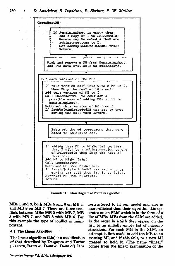
(c) FIGURE 15. Example of nonoptimal Lin execution. (a) Renumbered
data dependency graph. (b) Renumbered microoperation conflicts. (c) Execution trace.
through the DDG is of length 4. To keep data-dependent MBs in different MIs, we need at least four MIs, and therefore 4 is the theoretical lower bound. A fifth MI is necessary due to the conflict between MB 5 and MB 6.
A PASCAL procedure for the Lin algo- rithm can be seen in Figure 14. In order to run, this procedure must be supported by the predefined types MOBUNDLE and INSTR, as well as by the following routines: AppendI, CanPrecedeI, CanAddToUnpre- cedableI, CanAddToPrecedableI, AddToI, and InsertIAtTop.
Though the Lin algorithm performed op- timally in the example of Figure 13, it is not guaranteed to do so. Figure 15a shows the DDG in Figure 12 renumbered. Since Lin is a first-come, first-served algorithm, this will have an effect on the performance.
Figure 15c shows the performance of Lin on this DDG. MBs 1 and 2 are not data dependent on each other and do not con- flict, and so are combined into MI I. MB 3 is not data dependent on either of the pre- vious MBs and so can be added to MI I if it does not conflict with the MBs. However MB 3 does conflict with MB 1, so a new MI must be formed. In this case, as mentioned previously, we form a new MI above the already formed MI. MB 4, data dependent on MB 1, is placed in MI 3. MB 5, data dependent on MB 3, can be placed no ear-
lier than MI 2. It conflicts with MB I in MI 2, however, and is therefore placed in MI 3. MBs 6, 7, and 8 are placed next, forming three new MIs, as in the foregoing example. The resulting microprogram is six microin- structions long and is thus nonoptimal.
How can this algorithm be made always to produce optimal results? This can be accomplished only by running the algo- rithm with the MBs in the SLM in every legal order (every order that does not vio- late data dependency) until an optimal list of MIs is obtained. However it is imprac- tical to do this because the many redundant calculations involved make. this approach much slower than the BAB algorithm of Section 4.3.
Weak dependencies are handled in a straightforward manner by the Lin algo- rithm. They are tested when Lin starts to check for conflicts with the rise limit. The current MB was found to be dependent on some MB(s) in the rise limit. Any strong dependency here means the current MB cannot be added to the rise limit MI. In the PASCAL example of Figure 14, this analy- sis is done by CanAddToUnprecedableI.
4.2 The Critical Path Algorithm
Critical path algorithms for ~dcrocode com- paction were introduced by Ramamoorthy
Computing Surveys, VoL 12, :No. 3, September 1980

284 • D. Landskov, S. Davidson, B. 8hriver, P. W. Mallett
Early Partition Late Partition Critical Partition Frame
1 1 , 2 , 7 2 2 2 3,8 1,3 3 3 4 4,7 4 4 5,6 5,6,8 5,6
(a)
Revised Critical Partition Frame
I 2 2 3 3 4 4a 5 4b 6
Co)
Noncritical MBs
1,7,8
List of MIs After Adding Noncritical MB:
1 7 8 Frame
I 1,2 1,2 1,2 2 3 3 3 3 4 4,7 4,7 4a 5 5 5,8 4b 6 6 6
(c)
FIouR~. 16. CPath execution of the example in Figure 12. (a) Forming tl~e critical partition. (b) The revised critical partition. (c) Adding the noncritical MBs.
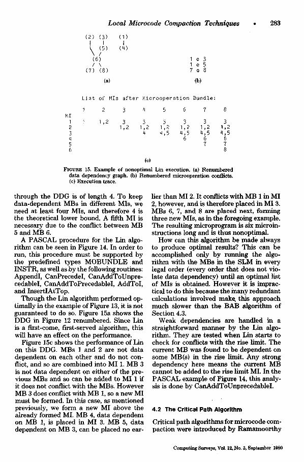
and Tsuchiya [RAMA74]. Their technique was similar to the critical path approach to processor scheduling [RAMA69, GONZ77]. The following critical path algori thm (CPath) attempts to identify MBs that must be executed at a certain time in order for the list of MIs to be optimal. The MBs chosen are those which are on a longest path (the critical path) through the DDG. As noted, the minimum possible number of MIs is just the length of a longest path. If any MB on this path is delayed beyond the MI where it first becomes data available, any MB following will also be delayed, and the number of MIs in the list will be in- creased.
CPath proceeds as follows (see Figure 16). The first s tep is to create an ea r ly pa r t i t i on (EP). Each time frame of the EP contains those MBs that could be executed in that time, at the earliest. Figure 16a
Computing Surveys, Vot 12, No. 3, September 1990
shows the EP for the example SLM. Since MBs 1, 2, and 7 are not data dependent on any other MB, they can be executed in frame 1. MBs 3 and 8 are each dependent on an MB in frame 1 and thus can be executed in frame 2 at the earliest. MB 4 is dependent on MB 3 in frame 2, so it can be executed in frame 3. Notice that although MB 4 is also dependent on MB 1, i t must be placed in frame 3; otherwise it could execute at the same time as one of its ancestors in the DDG. An MB must be placed in the frame of the EP after the frame of its latest ancestor.
MB 5, being dependent on MB 4, is placed in frame 4. The same is true for MB 6. Notice that data dependencies alone de- termine the placement of MBs in the EP. Conflicts are resolved later.
The final early partition is of length 4. This is the length of the longest path
Local Microcode Compaction Techniques , 285
through the DDG and defines the minimal number of MIs in the list of MIs.
The next step is the creation of a la te pa r t i t ion (LP). In the LP the latest possi- ble timings of the MBs are displayed. The LP is created by moving backward through the SLM. No MB is dependent on MB 8, so MB 8 can be the last MB executed. It can therefore be placed in time frame 4 of the LP. Again, the length of the LP is just the length of the longest path through the DDG.
The next MB placed is MB 7. Since MB 8 is dependent on MB 7, MB 7 must be placed in the time frame before MB 8, or frame 6. No MBs are data dependent on either MB 5 or 6, and so these MBs can be placed in time frame 4. Since MBs 5 and 6 are dependent on MB 4, MB 4 must be placed in frame 3. MBs 1 and 3, both ances- tors of MB 4, must be placed in the frame preceding that of MB 4, flame 2. Finally, MB 2, the ancestor of MB 3, is placed in frame 1. The resulting LP is in Figure 16a. If the data dependency graph is represented by a matrix, the LP can be created by applying the EP algorithm to the transpose of the graph matrix.
The construction of these partitions fa- cilitates the identification of MBs on the critical path of the DDG. These MBs, called critical MBs, are just those with the same early and late timings. It is trivial to construct a cr i t ical pa r t i t ion (CP) by ex- amining the EP and LP. The critical parti- tion for our example is shown in Figure 16a. MBs 2, 3, 4, 5, and 6 are critical here. The length of the CP is, of course, the length of the longest path through the DDG, in this case 4. The CP serves as a skeleton of our final list of MIs.
Since the CP was constructed by consid- ering only data dependencies between MBs, two MBs in the same frame of the CP may conflict. And since the frames of the CP will serve as a basis for MIs in the list of MIs, conflicting MBs in a frame must be separated. In frame 4 of our example CP, MBs 5 and 6 conflict. A frame with conflict- ing MBs must be split so that the MBs in the resulting subframes do not conflict. In our example frame 4 is trivially split into subframes 4a and 4b, each containing a single MB. The result of this process, the r ev i s ed cr i t ical pa r t i t i on (RCP), is
shown in Figure 16b. We will continue to talk in terms of frames because they pro- vide a link between the RCP and the early and late partitions. As seen from frame 4, one frame can contain several microinstruc- tions. A subframe is a partially complete microinstruction. Either FonnCIs or a sim- ilar algorithm must be used to form the subframes.
The next and final step of CPath is to add the noncritical MBs to the RCP, form- ing the final list of MIs. The noncritical MBs here are MBs 1, 7, and 8. We search the RCP from the frame containing the MB in the EP to the frame containing the MB in the LP for a microinstruction to which the noncritical MB can be added. In the case of MB 1, we start with frame 1 and end with frame 2. If the MB cannot be added to any of the frames within this range, a new subframe is created. This subframe is posi- tioned at the end of the last frame in the range. The MB is placed in this subframe, creating an MI with only one MB. In our example, however, MB 1 can be added to the MI in frame 1 without difficulty. Figure 16c, column 1, shows the list of MIs after MB 1 is added.
MB 7 can be added to either frame 1, 2, or 3. It cannot be added to frame 1 because' of a conflict with MB 2 or to frame 2 because of a conflict with MB 3. It can be added to frame 3 however.
The final MB to add is biB 8. If we used the EP to indicate the earliest frame to which MB 8 could be added, we would find that it could be added to frame 2. If it were added to frame 2, however, it would be placed before MB 7, thus violating the data dependency constraint. Therefore we must revise the EP to place all MBs dependent on MB 7 after MB 7. The earliest timing of MB 8 becomes frame 4, which is also the latest possible timing. We at tempt to add MB 8 to the subframes of frame 4, in turn, and find that MB 8 can indeed be placed in subframe 4a. Column 8 of Figure 16c shows the final list of MIs, which is of length 5 and therefore optimal.
The critical path algorithm, like the lin- ear algorithm, does not always produce op- timal results. This can be shown by consid- ering our example DDG, plus the following conflict: 4 c 7. The early, late, critical, and revised critical partitions remain the same
Compttting Sm~veys, VoL ~No. 3~ Sel~mnber 1980

286 D. Landskov, S. Davidson, B. Shriver, P. W. Mallett
List of MIs a£ter adding Noncritical MB:
" 1 7 8 Frame , F r a m e ~ ,
1 1,2 1 1,2 1,2 2 3 2 3 3 3 q 3a . 4 4 4a 5 3b 7 7 4b 6 t l a 5 5,8
4b 6 6
FIGURE 17. Example of nonoptimal CPath execution: Adding the noncritical MBs.
as fo~ the foregoing example. However the result of adding the noncritical MBs is changed. MB I can be added to frame 1, as before. MB 7, however, cannot be added to frame 3 because of a conflict with MB 4. Since frame 3 is the latest time frame of MB 7, a new subframe must be created after frame 3 and before frame 4a. In col- umn 7 of Figure 17 MB 4 is in frame 3a and MB 7 is in frame 3]).
As before, MB 8 must be placed within frame 4. It can be placed in frame 4a, giving the list of MIs of•Figure 17, colUmn 8. This list of MIs is of length 6 and is nonoptimal, as can be seen by moving MB 8 to frame 4b and MB 7 to frame 4a, giving the list of MIs of Figure 18. This list of MIs is five microin- structions long and is optimal.
This example shows the weakness of the critical path algorithm. Two adjacent subframes may be composed into a single microinstruction but are not because of the rigid boundaries between frames imposed by the algorithm. This problem does not arise from the first-come, first-served na- ture of the algorithm. The foregoing non- optimal list of MIs would have been ob- tained for any ordering. Both an exhaustive search of the possible orderings and an attempt to cc,'nbine adjacent frames would be necessary to make this algorithm opti- mal.
Frame MI
FIGURE 18. Figure 17.
I 1,2 2 3 3 4 4a 5,7 4b 6,8
An optimal solution to•the problem of
Weak dependencies are handled in CPatl~ by putting MBs in the same frame of the E P a n d LP as the parents on which they are weakly dependent.
• 4 .3 The Branch and Bound Algorithm
The third algorithm to be considered is branch and bound (BAB), a general class of tree,searching scheduling a~gorithms. Yau, Schowe, and Tsuchiya [YAU74] were the first todescribe the application of this technique to micr6code compaction.
In BAB, a tree is built, the nodes of which correspond to micrginstructions. A path from the root of thee tree to a leaf is an ordering of MIs, and thus a list of MIs. The tree branches whenever there is more than one mie_roinstruction that could be placed at a point in the list of MIs. A complete tree represents every possible microinstruction ordering.
There are two variants of this algorithm. The first is BAB exhaustive, in which every branch of the tree that could possibly lead to an optimal MB ordering is explored. The other is BAB heuristic, in which pruning is done to the tree. BAB exhaustive is an optimal algorithm, thus running in expo- nential time, while BAB heuristic is not guaranteed optimal and can be made to run in polynomial time.
The growth of the tree can be bounded even in BAB exhaustive. As in the other algorithms, calculate the lower bound on the number of microinstructions in the best possible ordering. (Remember that this is the longest path through the DDG.) A path through the BAB tree of this length repre- sents an optimal ordering, and the algo- rithm can stop once such a path is obtained.
Local Microcode Compaction Techniqueg • 287
The growth of the tree can be further bounded by remembering the length of the best (shortest) path found so far. If the length of an incomplete list of MIs is greater than or equal to this length, the current path needs no further consideration.
Like the critical path algorithm, the BAB algorithm gets its information on the data dependencies of an SLM's MBs through a DDG. The first step of the BAB exhaustive algorithm is the construction of a data ava i lab le se t (Dset). This is the set of all unplaced MBs that are not data dependent on any unplaced MB. The contents of the Dset change as execution of the algorithm progresses. The initial Dset (Dset 1) for our example in Figure 12 is 1, 2, 7 (just those MBs not dependent on any other MB).
The next step is to form microinstruc- tions from the MBs in the Dset. We wish to form only the largest possible MIs. These are called complete instructions (CIs). A complete instruction is defined as an in- struction to which no other MB in the Dset can be added (see Section 3). Thus a CI is not a subset of any other legal MI. CIs make up the nodes of the BAB tree so that a path through the tree (a list of MIs) is a list of CIs.
An algorithm for the identification of CIs is found in Section 3. For our example, the CIs are easily identified. For Dset 1, the CIs are 1, 2 (I1) and 1, 7 (I2). MBs 2 and 7 cannot appear together because of the con- flict between them. MB 1 by itself is a legal microinstruction but not a CI because it is a subset of I1.
At this point it is not known which of the CIs will lead to a better list of MIs. There- fore the tree must be split and each CI dealt with in turn. Figure 19 shows the execution of the BAB exhaustive algorithm. Each part of the figure shows one step. In Figure 19a the initial Dset, the CIs generated from it, and the tree produced by splitting the CIs are shown.
We built the BAB tree depth-first to allow us to find the length of some com- pleted paths which may enable us to cut off some other paths. Let us proceed with the left branch of the tree.
Calculate Dset 2 by first removing the MBs in I1 from Dset 1. This leaves MB 7 in the Dset. Next add the MBs that have
become data available to the Dset. At this point MB 3, data dependent on MB 2, becomes data available because MB 2 has been added to the tree. Note that MB 4 does not become data available because it is dependent on MB 3, which is still in the Dset at this point.
Since MBs 3 and 7 conflict, there are two single MB CIs that can be generated from Dset 2: I3, which consists of MB 3, and I4, which consists of MB 7. Split the tree again. Figure 19b shows the state of the tree at this point.
Again proceeding down the left branch, calculate Dset 3. This Dset consists of MBs 4 (dependent on MB 3) and 7. Since these MBs do not conflict, only one CI can be generated from this ]:)set, which consists of both MBs 4 and 7. Thus we do not branch here. The tree with this node added is shown in Figure 19c.
The new Dset (Dset 4) consists of those MBs dependent on MBs 4 and 7. All the remaining MBs fit this description, so Dset 4 contains MBs 5, 6, and 8. Since MBs 5 and 6 conflict, two CIs are formed from this Dset; one contains MBs 5 and 8, and the other contains MBs 6 and 8. Since there are two CIs, the tree branches, thus producing the tree of Figure 19d.
Pick I6, leaving MB 6 in the Dset. This Dset, Dset 5, obviously forms just one CI, I8. Adding I8 to the tree exhausts the MBs in the SLM, so the path from the root to I8 forms a list of MIs of elements I1, I3, I5, I6, and I8. Figure 19e shows the equivalent list of MIs, which is of length 5 and is optimal. However it does not reach the lower bound of length 4, and since there are more CIs to investigate, execution of the algorithm does not terminate. Mark the leaf of this path with a "P" to indicate that this is the best path tbund so far.
Now back up to Dset 4 and move down the right path, choosing I7. The new Dset, Dset 6, consists of MB 5, which forms one CI, I9. Add I9 to the tree (Figure 190, thus exhausting our list of MBs and producing a new list of MIs. Since this list of MIs is of length 5, which is no better than the first one produced, we throw this list of MIs away--indicated by placing an "X" below node I9.
The next incomplete path ends with node
Computing Surveys, Vol. 12, No. 3, September 1980
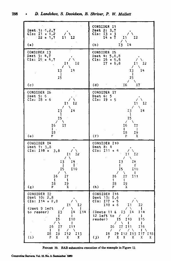
288 • D. Landskov, S. Davidson, B. Shriver, P. W. Mallett
Dset. 1~: '1 ,2,7 CIs:~ 11 = 1,2 I'\.
12 = I ,7 11 12
(a) i il
CONSIDER I3 Dset 3:4,7 tIs: 15 = 4,7 I \
II I2 / \
I3 I4 I
I5
(o) i i u ,
CONSIDER 16 Dset 5:6 CIs: 18 = 6 / \
11 12 / \
I3 14 I
15 / \
16 17 I. I8
(e) P
CONSIDER I4 Dset 7:3,8 Cls: II0 = 3,8 I \
11 12 / \
i3 I4 I l
I5 I10 / \
16 17 t I
18 19 (g) P x
CONSIDER I2 Dset 1 0 : 2 , 8 Cls: I14 : 2,8 / \
II I2 (Dset 9 left / \ I to reaOer) I3 14 114
i l I5 II0
/ \ I I6 I7 ' II I l I / \
18 I9 I12 113 (i) P X X X
CONSIDER II Pset 2:3,7 CIs: I3 = 3
I4 = 7
(b)
CONSIDER I5 Dset 4:5,6,8 CIs: I6 = 5,8
I7 : 6,8
(d)
CONSIDER I7 Dset 6:5 CIs: 19 = 5
(f)
CONSIDER 110 Dset 8:4 Cls: 111 : 4
/ \ II I2
/ \ I3 I4
/ \ II I2
/ \
I3 14 I
15 / \
I6 I7
/ \ II I2
/ \ I3 I4 i
I5 / \
I6 I7 i l I8 I9 P X
I \ II I2
/ \ I3 I4 I I' 15 ii0
/ \ I I6 I7 I11 i I I8 I9
( h ) P x i
CONSIDER I16 Dset 13:5,6 CIs: I17 = 5 / \
I18 = 6 II I2 /\ I
(Dsets; 11 & .I3 I4 I14 12 left to / / I reader) 15 110 I15
/ \ I I I6 I7 I11 I16 I I I\ I\
I8 I9 I12 I13 I17 I18 (j) P x x x x x
FIOURE 19. BAB exhaustive execution of the example in Figure 12.
Computing VoL 12, .3,

Local Microcode Compaction Techniques
I4. Remember from Figure 19b that the Dset when this node was added to the tree was 3, 7. I4 corresponds to the choice of the CI consisting of MB 7. Thus the remaining Dset consists of MB 3. The new Dset, Dset 7, consists of the MBs dependent on MB 7 (MB 8) and MB 3. Dset 7 is shown in Figure 19g. Only one CI can be formed from this Dset. This instruction, I10, consists of both MBs 3 and 8. It is added to the tree after I4, as shown in Figure 19g.
Figure 19h shows the addition of the next CI, I l l . There is nothing new in this step, or until the state shown by the tree in Figure 19i. I12 consists of MB 5. At this point we have placed all MBs except MB 6 in 5 MIs. Since we have equaled the best path length, with one more MB to place, we know we can do no better than the list of MIs shown in Figure 19e, and we cut off this path. The same holds for the path ending with I13, except that here we have placed all but MB 5.
Next back up to I2, constructing I14 out of Dset 10 as shown in Figure 19i. The end of this path, and the complete BAB tree, is shown in Figure 19j. As in the case of the path ending with I12 and I13, at nodes I17 and I18 we have equaled the best path length so far without placing all of the MBs in the SLM. Therefore we can cut off, as shown by the X's under nodes I17 and I18. At this point there are no more incomplete paths, and the algorithm has completed. The list of CIs found is the one shown in Figure 20. This list of CIs is of optimal length.
In BAB weak dependencies are handled b y the FormCIs algorithm.
CI MBs
FIGURE 20.
11 1,2 I3 3 I5 4,7 I6 5,8 18 6
The solution ~und m Figure 19.
4.4 Branch and Bound Heuristics and List Scheduling
Since the branch and bound algorithm con- siders all possible combinations of MBs, it is guaranteed to produce an optimally im-
• • 2 8 9
proved microprogram. The cost, however, is exponential since all of the paths of the tree must be explored. It is possible to find a heuristic that will prune the BAB tree without affecting the resulting micropro- gram too adversely. Such a heuristic will, of course, not always produce optimal re- sults, but it should save a great deal of time. Tests of different heuristics have been re- ported by Mallett [MALL78].
Consider the following heuristic: Instead of examining each complete instruction generated from a Dset, examine only the "best" CI, where the best instruction is determined by some metric. This heuristic requires only an amount of time that grows polynomially with the number of MBs in the SLM.
An algorithm that executes in this man- ner is an example of a list scheduling algo- rithm [ADAM74, FISH79]. Although list scheduling algorithms can be considered a special case of branch and bound algo- rithms, they are important in their own right. A list scheduling algorithm can be programmed much more easily than a full branch and bound algorithm. The tree of CIs is just one branch, and no bounds checking need be done. Furthermore, the complexity of FormCIs is greatly reduced, as noted in Section 3.2.
MB Weight
1 3 2 4 3 3 4 2 5 0 5 0 7 I 8 0
FIGURE 21. MB weights for the example in Figure 12 (number of descendants in DDG).
The weighting function used in forming the complete instruction affects the opti- mality of the compaction. Extensive tests of different functions were reported by Fisher [FISH79]. We present an example using a function proposed by Wood [WooD78].
The metric used by Wood is as follows. Assign a weight to each MB in the DDG. The weight of an MB is the number of descendants of that MB (direct or indirect)
Computing Surveys, VoL 12, No. 3, September 1980

290 • D. Landsko~ S. Davidson, B. Shriver, P. W. Mal~tt
Dset Contents Complete Inst. List of ~
I 1,2,7 2,1~, ~ ~2,1
2 3,7 3 2,1 3
3. 4,7 4,7 2,1 3
4,7
4 5,6,8 5,8 2,1 (First-Come, 3 First-Served) 4,7
5,8
5 6 6 2,1 3
4,7 5,8 6
FIGURE22. Lmtschedulingexecutionoftheexamplein Figurel2.
Mls
in the DDG. Figure 21 gives the weights of the MBs in our example. MB I has a weight of 3, since MBs 4, 5, and 6 are its descen- dants. MB 2 has a weight of 4, since its descendants are 3, 4, 5, and 6. MBs with no descendants, such as MB 8, are assigned a weight of 0.
Execution proceeds as follows (see Figure 22). Compute a Dset from the DDG. Find the MB in the Dset with the highest weight. Add it to the MI, which is initially empty. Then find the MB with the second highest weight. If this MB does not conflict with any MB already in the MI, add it. Repeat until all the MBs in the Dset have been examined. The resulting MI is the CI with the highest weight. Add this MI to the list of MIs and compute a new Dset. Repeat until all of the MBs in the SLM have been placed.
In Figure 22, Dset I contains MBs 1, 2, and 7. MB 2 is the MB of highest weight and is placed first in the CI. MB I has the second highest weight and can be added to the CI without conflict. The remaining MB in the Dset, MB 7, cannot be added to the CI because of a conflict between MBs 2 and 7, and so the first instruction in the list of MIs is 2, 1. The construction of the rest of the list of MIs is straightforward. In this case the final list of Mis is of length 5, is optimal, and is exactly the same as the list of MIs produced by the exhaustive variant of BAB.
Computing Surveys, Vol. 12, No. 3, S e p ~ 1980
4.5 Computationa! Complexity
In the past, the microcode compaction problem has had the reputation of being very complex [AO~.R76]. It was widely be- lieved that a program for automatic com- paction would be too expensive to run in a production environment. This reputation is well deserved in the optimal case. Compac- tion is in a class of difficult problems which includes such well-known elements as the "traveling salesman problem." But as with many of these problems, there exist practi- cal algorithms that can produce acceptable results for many applications.
NP is a well-known class of "difficult" problems [MACH78]. Problems in this class can be solved on a nondeterministic Turing machine in polynomial time. Certain prob- lems in N P are NP complete. If a polyno- mial time (deterministic) algorithm can be found to solve any problem that is NP complete, then a polynomial time algorithm can be found to solve every problem in the class. Since an algorithm with less than exponential time has never been found for an NP-complete problem, it is widely be- lieved that all NP-complete problems are of at least exponential complexity. We now show that microcod¢ compaction is at least as difficult as NP-complete problems.
In ULLM73 the unit time scheduling prob- lem is shown to be NP complete. This prob- lem is as follows:

Local Microcode Compaction Techniques • 291
Given
(1) a set S ffi { J1 , . . . , Jn} of jobs, (2) a partial order << on S, (3) that each job requires one time unit,
and (4) a number of processors, k
(up to k jobs may be executed at each time unit), minimize tmax, the total number of time units required, under the constraint that if J << J ' , then J ' does not execute until at least one time unit after J.
It is straightforward to restrict our model to this problem. Let the SLM correspond to S, let data dependency be <<, and let the number of fields in an MI be k, where each MB can be in any field. (This same proof is done for a slightly different model in DEWI76.) Thus, if microcode compaction can be solved in less than exponential time, so can all problems in NP complete.
An alternate approach to establishing the exponential complexity of microcode com- paction can be found in YAU74. It should be pointed out that some articles in the literature have claimed to have less-than- exponential solutions to the optimal com- paction problem. All of these claims have been shown to be invalid.
Nonoptimal algorithms do not have to be exponential. The critical path, linear, and list scheduling algorithms work in polyno- mial time. It should be noted that the name linear does not imply that this algorithm has linear complexity but rather that the SLM is processed one MB at a time.
That the linear algorithm runs in poly- nomial time can be shown by considering the worst case SLM, wherein there are no data dependencies between MBs and where each MB conflicts with each other MB. In this case each already placed MB must be examined in order to ascertain that the new MB is not data dependent on any MB in the list of MIs. That is, i - 1 checks for data dependency must be done for the ith MB. The total number of checks done for an n MB SLM is therefore (n - 1)n/2. Each already-placed MB must be checked for conflict during the search for an MI to which the MB can be added. Again, for an n MB SLM, (n - 1)n/2 checks for conflicts must be done. Therefore n ~ - n compari- sons must be done between MBs in this
worst case, showing that the complexity is O(n2).
A branch and bound algorithm with suit- able heuristics is competitive with the other algorithms.
Extensive tests which support these con- clusions are reported in MALL78. In one test of an SLM of 96 MBs (231 MOs), for example, Lin compacted to 55 MIs using 309 MO-to-MO comparisons, CPath com- pacted to 54 MIs using 376 comparisons, and a BAB heuristic restricted to list sched- uling compacted to the optimal 50 MIs using 491 comparisons. The execution times on a Honeywell 68/80 processor (MUL- TICS) were 6.7 seconds, 11~ seconds, and 7.5 seconds, respectively. By contrast, an exhaustive BAB compaction required 183,364 comparisons to find the optimal 50 MIs and ran in 2629 seconds.
One practical factor affecting the execu- tion times of compaction programs is often overlooked. Because branches and entry points (i.e., labels) are common inmicro- programs, the typical SLM is not very long.
4.6 Register Allocation
The previous sections on compaction algo- rithms do not address the problem of allo- cating registers. This makes the presenta- tions easier to understand. Furthermore, many applications do not need the compac- tion routine to allocate registers. Spurred by the rapid drop in the cost of high-speed memory, the trend in computer architec- ture is to include more and more registers for microprogramming. If there are more registers than microprogram variables, each variable can be allocated a register before compaction, and reallocation need never be done.
The register allocation problem is as fol- lows. In addition to process registers, most microprogrammable processors have a lo- cal store. Data can be moved back and forth between the registers and local store. If there are more variables than registers, registers must be reallocated during the execution of the program. To reallocate a register, the value of the old variable must be saved in local store (if the register has changed value), and the value of the new variable must be loaded from local store (if it is needed). The difficulty with register
Computing Surveys~ VoL 12, No. 3, September 1980
292 • D. Landskov, S. Davidson, B.
reallocation is deciding which variables to reaUocate when a variable needs a register and there are no more unailocated (f~ee) registers. The wrong choice of variables can necessitate extra reallocations later.
Register allocation can be incorporated into the compaction algorithms presented here by considering variables as unbound resources. The variable-to-register binding must be maintained in a separate data structure. Whenever a register reallocation becomes necessary, the different possible reallocations correspond to different MB versions. Store and load microoperations must also be added to perform t h e reallo- cation. The register allocation problem is discussed at length in DEWI76.
It should be noted that register allocation also-affects global analysis. Since register allocations are maintained between SLMs as well as within them, an SLM is often constrained by initial and final register al- locations. Under this constraint the order in which SLM compactions are performed is important. An unconstrained SLM may compact to fewer MIs than its constrained counterpart. Thus the most critical SLMs (inside loops, say) should be compacted first.
5. CONCLUSIONS
Linear analysis compaction algorithms are easy to write, and they run in a reasonable amount of time. However they can only operate on SLMs in sequential form, and their results depend orL the order of the microoperation bundles in the SLM. It is easy to construct an example for which linear algorithn~ produce more MIs than necessary.
Critical path, branch and bound, and list scheduling algorithms operate on the SLM in graph form. Having to build a graph does not significantly increase execution time. The graph building program is also easy to write, although the compaction algorithms themselves are not straightforward to pro- gram. Critical path algorithms have diffi- culties with the rigid boundaries they im- pose between frames. These kinds of algo- rithms do not seem to be the best approach for microcode compaction.
Branch and bound algorithms can be ex- haustively run to find optimum solutions (for the minimization of the number of MIs
Computing storeys, Vol. 1~ No. S, September
Shriver, P. W. Mallett
for the SLM), but doing so is prohibitively expensive. List scheduling algorithms and branch and bound algorithms with suitable heuristics can compact approximately as fast as linear analysis algorithm.s and are not nearly as dependent on the original order of the microoperations. Furthermore the probability of an optimal branch and bound compaction can be adjusted by changing the heuristics. List scheduling programs are easier to write than branch and bound programs.
These algorithms can work with realistic processor models. It is true, however, that realistic hardware details make the algo- rithms harder to program. In particular, whenever microoperations have a choice of resources (registers, fields, e tc . )where the choice can have an adverse effect on later execution, the complexity of the compac- tion problem increases. Further investiga- tion of modeling processor control is needed.
Exhaustive comparisons of the compac- tion algorithms have shown that all four kinds are capable of producing acceptable compactions in a reasonable amount of time. Often the small size of an SLM makes local compaction trivial. Although many issues merit further study, especially with regard to global compaction, practical com- pilation of horizontal microcode is feasible.
GLOSSARY Compaction--Production of a sequence of mi-
croinstructions that is semantically equivalent to a given ordered set of microoperations. Most compaction~ try to minimize execution time.
Compatible--Having no resource conflicts. Complete instruction (CI)--Instruction to
which no other MB in the Dset can be added. Confliet--Attempt to share an unsharable re-
s o u r c e .
Data available--Addition of an MO to a par- ticular MI in a list of MIs does not violate data integrity.
Data dependent (dd)--mol dd mo/if moy is directly data dependent either on moi or on an MO which is itself data dependent on mol.
Data dependency graph (DDG)--Graphical representation of a partial order over the MOs of an SLM.
L o c a l M i c r o c o d e C o m p a c t i o n T e c h n i q u e s
D a t a i n d e p e n d e n t ~ N o t data dependent.
D a t a i n t e r a c t i o n - - T w o MOs have a da ta in- teraction if an input operand of one is also an output operand of the other or if they have an output operand in common.
D i r e c t l y d a t a d e p e n d e n t (ddd)--mo~ d d d moi if mol precedes moj in the given MO ordering, if moi and moy have a data interaction, and if no nonempty chain of directly data dependent MOs exists between them.
F ie ld - -Col lec t ion of bits in the control word tha t controls a primitive machine activity.
G l o b a l a n a l y s i s - - A n a l y s i s that considersmore than one SLM.
H o r i z o n t a l a r c h i t e c t u r e - - A r c h i t e c t u r e tha t allows many MOs in the same MI.
Host m a c h i n e - - C o m p u t e r tha t a given micro- program is designed to control.
L o c a l a n a l y s i s - - A n a l y s i s tha t considers one SLM.
M i c r o i n s t r u c t i o n (MI)--Specif icat ion of all MOs tha t are to s tar t during one machine cycle, i.e., a conflict-free set of MOs.
M i c r o o p e r a t i o n (MO)--Specif icat ion of a primitive machine operation.
Microoperation b u n d l e ( M B ) - - A set of one or more MOs tha t must be executed in the same MI.
M i c r o p r o g r a m - - S e q u e n c e of microinstruc- tions.
R e m a i n i n g D s e t ( R D s e t ) - - S e t of all remain- ing MBs.
R e m a i n i n g M B - - M B in a Dset that has not yet been included in or excluded from the current microinstruction.
O r d e r p r e s e r v i n g - - T w o MOs are order pre- serving if they can be placed in the same MI (ignoring resource conflicts) such tha t for ev- ery resource causing a data interaction be- tween them, the MO that is earlier in the SLM finishes with the resource before the other MO star ts to use it.
P a r a l l e l - - T w o MOs which are order preserving and conflict-free are parallel.
P a r t i a l i n s t ruc t ion - -Mic ro ins t ruc t ion for which remaining MBs exist.
P o l y p h a s e t i m i n g - - A n MI cycle is composed of dist inct phases; MOs are active only in specified phases.
• 293
P o t e n t i a l l y c o m p l e t e i n s t r u c t i o n - - P a r t i a l instruction tha t is not a subinstruction to any known complete instruction.
S t r a i g h t - l i n e m i e r o e o d e s e c t i o n (SLM)--Or- dered collection of MOs with no entry points except at the beginning and no branches ex- cept possibly at the end.
S t r o n g l y d e p e n d e n t ( s d ) - - I f moi d d d mo s and it is known tha t moi is not weakly dependent on moi, then mos is strongly dependent on moi (moi sd moj).
Subinstruction--A part ia l instruction is a sub. instruction to an instruction if the union of the part ia l instruction and all MBs tha t can potential ly be added to i t is a subset of the instruction.
T r a n s i t o r y - d a t a r e s o u r c e - - S t o r a g e resource whose contents can become undefined at the terminat ion of an MI in which i t has been given a value.
V e r t i c a l a r c h i t e c t u r e - - O n e tha t allows only a few MOs, or one M 0 , in an MI.
W e a k l y d e p e n d e n t (wd) - -Given two MOs, moi and moj, then moj is weakly dependent on moi (moi w d rnoj) if moj is directly data depen- dent on mo~, and if for every resource causing a da ta interaction between them, moi finishes with the resource before moj s tar ts to use it.
ACKNOWLEDGMENTS
The authors wish to thank the referees for their help- ful comments. We are also grateful to Julie Jackson for her many hours of assistance and to the other volunteers who gave of their time.
ADAM74
AGER76
AGRA76
BARN78
COFF76
REFERENCES
AVAM, T. L., CHANDY, K. M., AND DICK- SOS, J.R. "A comparison oflis~ schedules for parallel processing systems," Commun. ACM 17, 12 (Dec. 1974), 685-690. AG~.RWALA, T. "Microprogram optimi- zation: A survey," IEEE Trans. Comput. C-25, 10 (Oct. 1976), 962-973. AGRAWALA, A. K., ANY RAUSCHER, T. G. Foundations of microprogramming, Academic Press, New York, 1976. BARNES, G. E. "Comments on the identification of maximal parallelism in straight-line microprograms," IEEE Trans. Comput. C-27, 3 (March 1978), 286- 287. COFFMAN, E. G., JR., Eb. Computer and job-shop scheduling theory, Wiley, New York, 1976.
Computing Sm-veys, VoL 12, No. 3, September 1980

294 • D. Landskov, S. Davidson, B. Shriver, P. W. Mallett
DASG76 DASGUm, S., AND TARTAR, J. "The RAMA69 idant'dlcation of maximal parallelism in straight-line microprograms," IEEE Trans. Comput. C-25, 10 (Oct. 1976), 986- 992. DASOV~A, S. "Comment on the identi- fication of maximal parallelism in straight- RaMA74 line microprograms," IEEE Trans. Corn- put. Co27, 3 (March 1978), 285-286. DASOm~rA, S. "The organization of mi- croprogTam stores," ACM Comput. Surv. SHIn73 11, 1 (March 1979), 39-35/ DAVIDSON, S., AND SHRFeEE, B.D. "An overview of fn, mware engin~ing," Corn- TABA74 purer 11, 5 (May 1978), 21-33. DEWIer, D.J. "A control word model for detecting conflicts between micr0opera- tions," in Proc. 8th Annual Workshop on Microprogramming (ACM), 1975, pp. 6- TOKO77 12. DEWITT, D.J . "A machine-independent approach to the production of horizontal microcode," Ph.D. dissertation, Univ. Michigan, Ann Arbor, June 1976; Tech.
• Rep. 76 DT4, Aug. 1976. FISHER, J. A. The optimization of horizon- TOKo78 tal microcode within and beyond basic blocks: An application of proeessor sched- uling with resources, U.S. Dept. of Energy Report, Mathematics and Computing COO. 3077-161, New York Univ., Oct. 1979. Tsuc74 GONZALEZ, M. J., JR. "Deterministic processor scheduling," ACM Comput. Surv. 9, 3 (Sept. 1977), 173-204. KLEIn, R. L., AND RAMAMGoRTHY, C. V. "Optimization strategies for micropro- grams," IEEE Trans. Comput. C-20, 7 (July 1971), 783-795. K~Em, R. L. "A representation for the analysis of microprogram operation," in Proc. 7th Annual Workshop on Micropro- WOOD78 gramming (ACM), 1974. MACHTEY, M., AND YOUNG, P. An intro- duction to the general theory of algo. rithms, North-Holland, New York, 1978. MALLETT, P. W., AND LEWIS, T. G. "Con- WOOD79 sidarations for implementing a high level microprogramming language translation system," Computer 8, 8 (Aug. 1975), 40-52. YAu74 MALLET% P.W. "Methods of compacting microprograms," Ph.D. dissertation, Univ. Southwestern Louisiana, Lafayette, Dec. 1978,
DASO78
DASG79
DAVI78
DEWI75
DEWI~
FISH79
GONZ77
KLEI71
E~EI74
MACH78
MALL75
MALL78
ULLM73
RAMAMOOIVI'HY, C. V., AND GONZALEZ, J., JR. "A survey of techniques for rec-
• o ~ n g parallel processable streams in computer programs," in Pro¢. 1960AFIPS Fall Joint Computer Conf., AFIPS Press, Arlington, Va., pp. 1-15. RAMAMOORTHY, C. V., AND TSUCHIYA, M. "A high-leval language for horizontal microprogramming," IEEE Trans. Corn- put. C-23, 8 (Aug. 1974), 791-801. SHmVER, B. D. "A description of the MATHILDA system," DA]MI PB-13, Univ. Aarhns, Denmark, 1973. TARANDEH, M., AND RAMAMOORTHY, C. V. "Execution time and memory optimi- zation in microprograms," in Proc. 7th An- nual Workshop on Microprogramming (ACM), 1974. ToXORO, M., TAMURA, E., TAKASE, K., AND TAMURA, K. "An approach to micro- program optimization considering resource occupancy and instruction formats," in Proe. lOth Annual Workshop on Micro- programming (ACM), Oct. 1977, pp. 92- 108. TOKORO, M., TAKIZUKA, T., TAMURA, E., AND YAMAURA, I. "A technique of global Optimization of microprograms," in Proc. l l th Annual Workshop on Microprogram. m/ng (ACM), 1978, pp. 41-50. TSUCHIYA, M., AND GONZALEZ, M. J., JR. "An approach to optimization of hor- izontal microprograms," in Proc. 7th An- nual Workshop on Microprogramming (ACM), 1974, pp. 85-90. ULLMAN, J. D. "Polynomial complete scheduling problems," in Proc. 4th Sym- posium on Operating Systems Principles; ACM Operating Syst. ReD. 7, 4 (Oct. 1973), 96-101. WOOD, G. "On the packing of micro-op- erations into micro-instruction words/' in Proc. l l th Annual Workshop on Micro- programming SIGMICRO Newsletter 9, 4 (Dec. 1978), 51-55. WooD, W.G. "The computer aided de- sign of microprograms," Ph.D. dissertation, Univ. Edinburgh, Scotland, 1979. YAU, S. S., SCHOWE, A. C., AND TSUCHIYA, M' "On storage optimization for horizon- tal microprograms," in Proc. 7th Annual Workshop on Microprogramming (ACM), 1974, pp. 98-106.
RECEIVED DECEMBER 1979; FZNAL REVISION MARCH 1980; ACCEPTED MAY 1980
Computing Surveys, Vo1.12, NO. 3, S e p t . bet H~0