Local level household income estimates 2014 summary report

Experimental Statistics: data being developed - These are new statistics being developed and have been published to involve users and stakeholders in their development and to build in quality and understanding at an early stage.

1

Scottish Government Experimental Statistics on Local Level Household Income Estimates

2014 – Summary of Results and Methodology

This paper provides a summary of the results from the local level synthetic income modelling

research for the year 2014 that has been prepared for the Scottish Government by Heriot Watt

University in association with David Simmonds Consultancy. The results provide gross household

income distribution estimates at Data Zone level for 2014 for use in housing affordability analyses.

Annex A provides a summary of the underlying modelling methodology used. An updated set of

2015 based figures are planned to be developed and published later in 2017.

An Excel workbook with Data Zone level results is available at http://www.gov.scot/Topics/Built-

Environment/Housing/supply-demand/chma. Data Zone level results will also be made available at

http://statistics.gov.scot/. For any further information please contact [email protected].

Important notes on the intended use of these income estimates:

- The household income estimates for 2014 have been produced for the purposes of updating the

Scottish Government Housing Need and Demand Assessment (HNDA) Tool.

-The estimates will also inform work on housing affordability more generally across different

tenures and different geographic areas of Scotland, and will help to support local authorities and

their partners in the production of Local Housing Strategies and other planning documents.

- It is important to note that the gross household income estimates are only one measure of income,

and should not be considered on their own without consideration of other local level information.

Users are strongly encouraged to use other detailed statistics such as the Scottish Index of Multiple

Deprivation or the Scottish Census to develop a basket of evidence and statistics to build up a

comprehensive picture of people and households in local areas.

- It is also important to note that the gross household income estimates are not intended to be a

measure of person-level income, they do not reflect household income adjusted by household size,

they do not reflect income levels after tax or after housing costs, they do not provide information on

wealth or assets, and they are not intended as a measure of income based deprivation. Not all

people in areas of low average gross household incomes will necessarily be deprived or in poverty,

and not all households in areas of high average gross household incomes will necessarily contain

people with high levels of personal disposable income or wealth.

Key Findings:

Note that:

- The income estimates presented below relate to gross household income, which covers total income

received by all adult members of a household, including welfare benefits, tax credits and housing benefit.

The estimates reflect total income before any deductions are taken off for income tax, national insurance

contributions and council tax etc.

- Local gross household income data allows household income levels to be compared to other data on

house prices and rental costs to ascertain levels of housing affordability across particular geographic areas.

http://www.gov.scot/Topics/Built-Environment/Housing/supply-demand/chma

http://www.gov.scot/Topics/Built-Environment/Housing/supply-demand/chma

http://statistics.gov.scot/

mailto:[email protected]


2

If you wish to use the income estimates for reasons other than housing affordability, you should be clear

about the methodology and limitations associated with the data and you may wish to seek advice first from

Scottish Government Centre for Housing Market Analysis ([email protected]).

- The figures presented are synthetic modelled estimates, in which data on income and household

characteristics from a national survey (the Scottish Household Survey) has been combined with associated

local area level data. The estimates generated for a given local area level are therefore the expected levels

of income in that area based on the household characteristics as measured by the associated local level

data, and are not aggregations of actual income data at a local level.

- Data zones are the key geography for the dissemination of small area statistics in Scotland and are widely

used across the public and private sector. They are designed to have roughly standard populations of 500

to 1,000 household residents, nest within local authorities, have compact shapes that respect physical

boundaries where possible, and to contain households with similar social characteristics. Findings below

relate to a total of 6,970 Data Zones out of 6,976 for which results are available1.

Mean weekly gross household income in Scotland in 2014 at a Data Zone level was estimated to

range between £337 (Glasgow Cowlairs and Port Dundas 01) and £1,559 (Stirling Dunblane East

05), with the national average being estimated to be £668 per week. A total of 3,800 (56%) of Data

Zones had a mean income less than the national average, with 3,170 (44%) having a mean income

greater than the national average.

Of the 100 Data Zones with the highest estimated average weekly gross household income (Data

Zones with average incomes of between £1,155 and £1,559), over two-thirds were located in the

following local authority areas: Aberdeenshire (18 Data Zones), West Lothian (15 Data Zones),

Aberdeen City (14 Data Zones), South Lanarkshire (12 Data Zones), and North Lanarkshire (8 Data

Zones).

Of the 100 Data Zones with the lowest estimated average weekly gross household income (Data

Zones with average incomes of between £337 and £429), over three-quarters were located in the

following local authority areas: Glasgow (52 Data Zones), Dundee (14 Data Zones), and

Renfrewshire (11 Data Zones).

Median weekly gross household income in 2014 at a Data Zone level was estimated to range

between £280 (Dundee Perth Road 05) and £1,431 (Stirling Dunblane East 05), with the national

average being £550. A total of 3,400 (49%) of Data Zones had a median income less than the

national average, with 3,570 (51%) having a median income greater than the national average.

The approximate proportion of households below 60% of median income in 2014 (i.e.

households with an income under 60% of the median value of £550 per week after adjusting for size

of household) was estimated to range from 0.3% in Fife Rosyth Dockyard and Castle to 52% in

each of Fife Masterton Central, Fife Masterton South, and Fife Middlebank. The national average

was estimated to be 15%. A total of 3,742 (54%) of Data Zones had proportion less than the

national average, with 3,228 (46%) having a proportion greater than or equal to the average.

1 There were two Data Zones in which there was insufficient source data, for example where demolitions have reduced the number of occupied households in these areas, as well as four Data Zones which were removed from the final results due income levels that appeared anomalously high – further information on these is provided in Annex A (see page 16).


3

Summary of results - Gross Household Income:

The income results include measures of mean and median gross household income along with the

proportions of households with incomes below a series of bands from £50 per week to £2000 per week.

The income estimates have been controlled for consistency to national level income levels from the Family

Resources Survey (FRS), and therefore provide local level information that is calibrated to existing national

level survey income estimates.

Mean weekly gross household income in Scotland in 2014 at a Data Zone level was estimated to range

between £337 (Glasgow Cowlairs and Port Dundas) and £1,559 (Dunblane East 05), with the national

average being estimated to be £668 per week. A total of 3,800 (56%) of Data Zones had a mean income

less than the national average, with 3,170 (44%) having a mean income greater than the average.

Of the 100 Data Zones with the highest estimated average weekly gross household income, over two-thirds

were located in the following local authority areas: Aberdeenshire (18 Data Zones), West Lothian (15 Data

Zones), Aberdeen City (14 Data Zones), South Lanarkshire (12 Data Zones), and North Lanarkshire (8

Data Zones). Of the 100 Data Zones with the lowest estimated average weekly gross household income,

over three-quarters were located in the following local authority areas: Glasgow (52 Data Zones), Dundee

(14 Data Zones), and Renfrewshire (11 Data Zones).

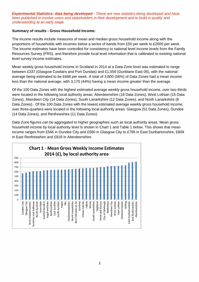
Data Zone figures can be aggregated to higher geographies such as local authority areas. Mean gross

household income by local authority level is shown in Chart 1 and Table 1 below. This shows that mean

income ranges from £566 in Dundee City and £580 in Glasgow City to £795 in East Dunbartonshire, £809

in East Renfrewshire and £818 in Aberdeenshire.


4

Median weekly gross household income in 2014 at a Data Zone level was estimated to range between

£280 (Dundee Perth Road 5) and £1,431 (Dunblane East 05), with the national average being £550. A total

of 3,400 (49%) of Data Zones had a median income less than the national average, with 3,570 (51%)

having a median income greater than the national average.

Summary of results - Households with an income of 60% less than the Median (i.e. households with

an income under 60% of the median value of £550 per week after adjusting for size of household):

A measure of relative low income poverty has been calculated for each Data Zone based on the modelled

synthetic income distribution estimates, which gives information on the proportion of households with an

income of 60% less than the median value of £550 per week. This is similar in concept to the former UK

Government target measure of relative low income, based on measuring households below 60% of the

median net equivalent income before housing costs, however differs in that the income thresholds have

been translated to a gross basis for the nine household types used in the model, based on an average

value from an OECD equivalence scale for each household type. This measure should therefore be

considered an approximate estimate only, but may be of interest for local level poverty related analysis.

Local Authority

Mean Gross

Weekly

Income (£)

Aberdeen City 722

Aberdeenshire 818

Angus 646

Argyll and Bute 635

City of Edinburgh 701

Clackmannanshire 654

Dumfries and Galloway 611

Dundee City 566

East Ayrshire 640

East Dunbartonshire 795

East Lothian 730

East Renfrewshire 809

Falkirk 679

Fife 648

Glasgow City 580

Highland 691

Inverclyde 616

Midlothian 718

Moray 679

Na h-Eileanan an Iar 661

North Ayrshire 613

North Lanarkshire 659

Orkney Islands 672

Perth and Kinross 697

Renfrewshire 640

Scottish Borders 633

Shetland Islands 737

South Ayrshire 646

South Lanarkshire 682

Stirling 741

West Dunbartonshire 597

West Lothian 725

Scotland 668

Table 1 - Mean Gross Weekly Income

Estimates 2014 (£), by local authority area


5

These figures are a helpful first step in illustrating poverty at local levels and how poverty differs across

Scotland on a gross household income basis, which is not currently available from over sources. We

welcome stakeholder views on how these figures can be developed, and this could involve work to

translate these figures into something more comparable to separate national level poverty and income

inequality figures that are currently produced using a more established National Statistics methodology2.

For monitoring national level trends we advise that the existing published National Statistics figures should

continue to be used as official measures of poverty and income inequality in Scotland.

The approximate proportion of households below 60% of median income in 2014 at a Data Zone level was

estimated to range from 0.3% in Fife Rosyth Dockyard and Castle to 52% in each of Fife Masterton Central,

Fife Masterton South, and Fife Middlebank. The national average was estimated to be 15%. A total of 3,742

(54%) of Data Zones had proportion less than the national average, with 3,221 (46%) having a proportion

greater than the national average.

The approximate proportion of households below 60% of median income in 2014 at local authority level is

shown in Chart 2 and Table 2 below. Proportions range from 0.11 in Aberdeenshire and Shetland Islands to

0.19 in Dundee City.

2 http://www.gov.scot/Topics/Statistics/Browse/Social-Welfare/IncomePoverty

http://www.gov.scot/Topics/Statistics/Browse/Social-Welfare/IncomePoverty


6

Summary of results – Lowest 25 and Highest 25 ranked Data Zones by gross household income,

with other income related variables:

Table 3 below presents the lowest 25 and highest 25 ranked Data Zones by gross household income, and

includes additional variables on the proportion of households under 60% of median income along with

SIMD16 variables.

It can be seen that for these Data Zones, areas ranked low or high for mean gross household income

generally have similarly rankings for low or high median gross household income. Data Zones ranked low

or high for income appear to contain some more varied rankings for the proportions of households under

60% of median income, and in terms of rankings for SIMD16 variables. This is not unexpected and is likely

to be due to a range of factors including that the mean and median income variables relate to gross

unequivalised income (i.e reflecting total household income), and therefore Data Zones with many smaller

sized households may by definition be more likely to have lower incomes compared to other measures.

Local Authority

Approx proportion of

households under 60%

of median gross

income, 2014

Aberdeen City 0.12

Aberdeenshire 0.11

Angus 0.16

Argyll and Bute 0.16

City of Edinburgh 0.13

Clackmannanshire 0.16

Dumfries and Galloway 0.17

Dundee City 0.19

East Ayrshire 0.17

East Dunbartonshire 0.12

East Lothian 0.13

East Renfrewshire 0.12

Falkirk 0.15

Fife 0.16

Glasgow City 0.17

Highland 0.14

Inverclyde 0.17

Midlothian 0.14

Moray 0.14

Na h-Eileanan an Iar 0.13

North Ayrshire 0.17

North Lanarkshire 0.16

Orkney Islands 0.14

Perth and Kinross 0.14

Renfrewshire 0.16

Scottish Borders 0.16

Shetland Islands 0.11

South Ayrshire 0.16

South Lanarkshire 0.15

Stirling 0.13

West Dunbartonshire 0.17

West Lothian 0.14

Scotland 0.15

Table 2 - Approximate proportion of households

under 60% of median gross income, 2014 - by

local authority area


7

However, broadly speaking this table shows that for most of these Data Zones, having a low average

income appears to correspond to having a higher than average proportion of households under 60% of

median income and a higher than average proportion of people income deprived from SIMD16. (And vice

versa).

This table is useful in emphasising that there can be some differences in rankings and values per Data

Zone depending on the choice of measure used, and so it is important to ensure that the most relevant

measure is used depending on the use being made of the data. For example mean or median gross

household income measures are likely to be appropriate to use when looking at housing affordability, i.e.

Table 3 - Data Zones ranked lowest 25 and highest 25 by gross household income - with other selected income related variables and rankings

2011 Data

Zone code 2011 Data Zone name

Local Authority

Area name

Mean

Gross

Weekly

Income (£)

Mean

Gross

Weekly

Income

(rank)

Median

Gross

Weekly

Income

(£)

Median

Gross

Weekly

Income

(rank)

Approx

proportion

of

households

under 60%

of median

gross

income

Approx

proportion of

households

under 60% of

median

gross

income

(rank)

SIMD16

Rank

SIMD16

Income

Domain

Rank

SIMD16

Percentage

of people

who are

income

deprived

Data Zones ranked 1 to 25 (i.e. lowest 25) on mean gross income:

S01010219 Cowlairs and Port Dundas - 01 Glasgow City 337 1 290 3 0.44 4 1,702 1,561 0.19

S01009150 Falkirk - Town Centre and Callendar Park - 02 Falkirk 345 2 285 2 0.21 642 895 858 0.25

S01010035 Laurieston and Tradeston - 05 Glasgow City 351 3 301 4 0.36 7 1,721 3,222 0.11

S01007693 Perth Road - 05 Dundee City 353 4 280 1 0.35 9 3,373 3,973 0.08

S01010262 City Centre East - 04 Glasgow City 364 5 310 8 0.25 104 377 322 0.32

S01010244 Carntyne West and Haghill - 03 Glasgow City 369 6 307 7 0.31 14 711 1,199 0.22

S01010226 Sighthill - 02 Glasgow City 375 7 313 12 0.38 5 1,562 843 0.25

S01010230 Roystonhill, Blochairn, and Provanmill - 03 Glasgow City 376 8 318 14 0.33 12 128 83 0.40

S01010023 Gorbals and Hutchesontown - 01 Glasgow City 378 9 324 19 0.26 56 311 588 0.28

S01010051 Parkhead West and Barrowfield - 03 Glasgow City 383 10 326 24 0.26 75 193 466 0.30

S01010138 Shettleston North - 02 Glasgow City 383 11 312 11 0.22 443 47 19 0.46

S01007706 City Centre - 06 Dundee City 384 12 329 28 0.31 15 4,397 4,807 0.06

S01010891 Greenock Town Centre and East Central - 02 Inverclyde 385 13 310 9 0.22 520 23 72 0.41

S01010873 Greenock West and Central - 04 Inverclyde 387 14 311 10 0.19 1,266 175 147 0.37

S01010362 Wyndford - 05 Glasgow City 387 15 316 13 0.19 1,094 30 20 0.46

S01009907 Strathbungo - 03 Glasgow City 388 16 325 22 0.24 221 993 1,274 0.21

S01007718 Hilltown - 05 Dundee City 389 17 326 23 0.24 149 813 661 0.27

S01011598 Cliftonville - 01 North Lanarkshire 389 18 323 18 0.24 188 8 29 0.44

S01009937 Pollokshaws - 05 Glasgow City 390 19 330 29 0.31 16 2,919 3,448 0.10

S01010361 Wyndford - 04 Glasgow City 391 20 324 20 0.25 141 33 44 0.43

S01009939 Carnwadric West - 01 Glasgow City 391 21 340 49 0.28 33 21 106 0.39

S01008929 Muirhouse - 01 City of Edinburgh 392 22 328 25 0.27 54 6 24 0.45

S01010309 Keppochhill - 01 Glasgow City 395 23 329 27 0.25 98 1,056 1,240 0.22

S01010323 Possil Park - 01 Glasgow City 396 24 336 40 0.24 192 7 4 0.55

S01010916 Port Glasgow Mid, East and Central - 01 Inverclyde 396 25 322 17 0.28 36 440 925 0.24

Data Zones ranked 6,947 to 6,971 (i.e. highest 25) on mean gross income:

S01011788 Kilsyth East and Croy - 03 North Lanarkshire 1,296 6,947 1,189 6,953 0.06 6,839 5,251 5,034 0.05

S01013095 Dunblane East - 02 Stirling 1,297 6,948 1,174 6,949 0.07 6,638 6,313 6,588 0.02

S01006519 Cults, Bieldside and Milltimber East - 02 Aberdeen City 1,306 6,949 1,160 6,944 0.07 6,680 6,404 6,680 0.02

S01006932 Westhill North and South - 04 Aberdeenshire 1,311 6,950 1,196 6,955 0.05 6,887 6,364 6,907 0.01

S01012947 Stewartfield West - 06 South Lanarkshire 1,312 6,951 1,192 6,954 0.06 6,855 6,068 6,929 0.01

S01006516 Cults, Bieldside and Milltimber West - 04 Aberdeen City 1,331 6,952 1,165 6,945 0.05 6,871 6,259 6,272 0.02

S01006913 Durno-Chapel of Garioch - 05 Aberdeenshire 1,333 6,953 1,215 6,956 0.03 6,964 5,895 5,636 0.04

S01011786 Kilsyth East and Croy - 01 North Lanarkshire 1,333 6,954 1,224 6,957 0.04 6,957 5,459 4,969 0.05

S01011776 Carrickstone - 06 North Lanarkshire 1,343 6,955 1,235 6,958 0.04 6,946 6,547 6,813 0.01

S01012606 Carluke East - 01 South Lanarkshire 1,352 6,956 1,247 6,961 0.03 6,963 6,106 6,921 0.01

S01008341 Mearns Village, Westacres and Greenfarm - 07 East Renfrewshire 1,356 6,957 1,246 6,960 0.04 6,933 6,748 6,482 0.02

S01006834 Stonehaven North - 05 Aberdeenshire 1,366 6,958 1,254 6,962 0.04 6,959 6,829 6,628 0.02

S01007420 Tullibody North and Glenochil - 06 Clackmannanshire 1,371 6,959 1,235 6,959 0.04 6,953 5,225 6,185 0.03

S01006829 Stonehaven South - 07 Aberdeenshire 1,371 6,960 1,256 6,963 0.04 6,940 6,563 6,764 0.01

S01006861 Banchory East - 03 Aberdeenshire 1,378 6,961 1,259 6,964 0.04 6,949 6,394 6,702 0.02

S01012951 Thorntonhall, Jackton and Gardenhall - 04 South Lanarkshire 1,403 6,962 1,292 6,966 0.03 6,968 6,512 6,919 0.01

S01013265 Bellsquarry, Adambrae and Kirkton - 03 West Lothian 1,406 6,963 1,292 6,967 0.04 6,960 6,212 6,445 0.02

S01006929 Westhill North and South - 01 Aberdeenshire 1,411 6,964 1,280 6,965 0.04 6,936 6,559 5,630 0.04

S01010174 Riddrie and Hogganfield - 03 Glasgow City 1,427 6,965 916 6,683 0.07 6,628 2,598 3,888 0.08

S01007142 Monikie - 06 Angus 1,435 6,966 1,302 6,968 0.03 6,967 6,135 6,545 0.02

S01006943 Garlogie and Elrick - 03 Aberdeenshire 1,475 6,967 1,351 6,969 0.03 6,966 6,713 6,949 0.01

S01011429 Allanton - Newmains Rural - 04 North Lanarkshire 1,510 6,968 1,383 6,970 0.03 6,965 4,817 5,803 0.03

S01008425 Currie West - 01 City of Edinburgh 1,552 6,969 954 6,761 0.09 6,104 6,763 6,860 0.01

S01006520 Cults, Bieldside and Milltimber East - 03 Aberdeen City 1,557 6,970 1,403 6,971 0.05 6,931 6,456 6,967 0.00

S01013098 Dunblane East - 05 Stirling 1,559 6,971 1,431 6,972 0.04 6,951 6,262 6,962 0.00


8

how total household incomes compare to house prices and rental costs which are largely measured at a

whole household level. However other types of analyses, including those focussing on poverty or income

of people rather than households, may be better placed to use a measure other than gross income.


9

Annex A – Methodology: Local Income Model and Income Distribution Estimates

This Annex provides details of the methodology and research that has been developed and carried out to

model and estimate local level income distributions by Heriot Watt University in association with David

Simmonds Consultancy.

Summary of General Approach

The methodology developed has been built on a blending of two previous approaches used in (a) the

Improvement Service / Scottish Government (Bramley & Watkins 2013) study on Local Income and Poverty

in Scotland3, and (b) the generation of Local Income data for Transport Scotland’s Transport Model for

Scotland (TMfS)4.

Method (a) was a 3-step process, entailing (1) developing predictive functions for income levels (or

proportions below thresholds) within the survey-based micro datasets with some area attributes attached;

(2) creating synthetic estimates at small area level using census and other sources for equivalent variables

to the predictors in (1); (3) controlling the predictions to actual values for types of Data Zone and local

authorities based on the ONS OAC classification5.

Method (b) relied on a disaggregation of households into 33 groups based on age, household composition,

and socio-economic level. Lognormal distributions were established for each group based on national data

from the major surveys, e.g. Understanding Society (UKHLS), and then local variations in the parameters of

these distributions were generated from additional data on the economic activity profile of these groups and

other local characteristics, again drawn from the Census and other local sources.

For the current set of research, Understanding Society (UKHLS) and Scottish Household Survey (SHS)

national survey sources have been used. SHS income data has been enhanced using an imputation

process, and also adjusted from a net to a gross basis. The final version of the income estimates have

been controlled for consistency with the Family Resources Survey (FRS) data for Great Britain and

Scotland in terms of overall income levels.

Monetary values are for 2014, scaled for consistency with the FRS values for Scotland in that year.

However, it should be emphasized that the base year for the analysis was 2011, using SHS data pooled

over the period 2009/10 to 2013/14 linked to 2011 Census and other data.

Underlying Assumptions and Hypotheses in Building the Model

Underlying the general approach suggested above are a number of assumptions or hypotheses about the

processes generating local income distributions, which it is useful to make explicit:

1) Household composition effects, particularly household size / type, age and occupation of main earner,

are important determinants of differences in household incomes.

2) Additional influences on income levels are likely to include levels of work participation per household,

prevalence of part-time work, and possibly factors like qualifications or ethnicity.

3 http://www.improvementservice.org.uk/assets/local-incomes-poverty-scotland.pdf 4 https://www.transport.gov.scot/our-approach/industry-guidance/land-use-and-transport-integrations-in-scotland-latis/# 5 http://webarchive.nationalarchives.gov.uk/20160105160709/http://www.ons.gov.uk/ons/guide-method/geography/products/area-classifications/ns-area-classifications/ns-2011-area-classifications/index.html

http://www.improvementservice.org.uk/assets/local-incomes-poverty-scotland.pdf

https://www.transport.gov.scot/our-approach/industry-guidance/land-use-and-transport-integrations-in-scotland-latis/

http://webarchive.nationalarchives.gov.uk/20160105160709/http:/www.ons.gov.uk/ons/guide-method/geography/products/area-classifications/ns-area-classifications/ns-2011-area-classifications/index.html

http://webarchive.nationalarchives.gov.uk/20160105160709/http:/www.ons.gov.uk/ons/guide-method/geography/products/area-classifications/ns-area-classifications/ns-2011-area-classifications/index.html


10

3) Housing and labour markets exert an influence on income levels, and distributions, at the level of travel-

to-work or housing market areas, for example through variables such as earnings, unemployment or house

prices.

4) Certain other attributes are known to be associated with higher or lower incomes, for example because

they reflect levels of consumption expenditure, and may act as effective proxy predictors, even though they

are not claimed to be causal influences on income; examples include car ownership, housing tenure

(especially social renting), large or small houses, or houses in top or bottom Council Tax bands.

5) Some of the above variables may be associated with income in non-linear or interactive fashion.

6) Because ‘like attracts like’, and because of market sorting processes, there may be spatial spillover or

dependence effects for incomes at small area level.

7) (a) For a given household type or occupation group, the distribution of household income at a small area

level (e.g. Data Zone) will be similar to the distribution at national level, but subject to some shifting up or

down to reflect point 2) above or other effects.

or (b) For a given household type/occupation group, households in a particular Data Zone will tend to be

drawn from a particular narrower stratum of income within the overall national distribution (i.e. assumes a

strong degree of income-based sorting).

8) For a given household type or occupation group, the distribution of household income at a small area

level may be best conceived and modelled as the sum of two or more distributions, for example a smooth

lognormal and a sharply peaked or stepped distribution which may arise from operation of the Benefits

system or the National Minimum Wage.

Much of the technical development work in the development phase of the modelling work was concerned

with exploring and testing these hypotheses, and finding a most appropriate practical way of reflecting

these findings in the model architecture.

Taking point 1), the significant predictive power of dummy variables for different household types and

occupational groups in general models of predicted income was tested. The overall proportion of variance

accounted for by between-group differences, based on the proposed typology or variants on it, was also

assessed.

For point 2), the inclusion or exclusion of these variables (e.g. unemployment) within general models to

predict income was tested, alongside the factors highlighted by point 1). These tests were conducted within

broad sub-groupings of households, e.g. separately for retirement age group and for households with one

or multiple adults.

For point 3), variables such as these were tested at higher geographical levels in the predictive models.

There may be issues and options about what geographical units to use to approximate to these ‘ideal types’

of labour market or housing market areas. In theory it might be possible to adopt a multi-level modelling

strategy here, but it may not be necessary unless we are hypothesizing more complex, varying processes

between different market areas, for example differential changes over time. Also such complexity may

make for significant difficulties in actually simulating local incomes. In practice, higher level market factors

are easiest to include at local authority level, but seem to be relatively marginal in their impact.

With regard to point 4), the test of whether to include such factors (e.g. car ownership) is whether they

improve prediction accuracy, not whether they are plausible as causal factors – some of these factors are


11

better seen as consequences rather than causes. Some may also be quite good proxies for the two ends of

the income distribution, ‘poverty’ and ‘wealth’, which previous experience (Bramley & Smart 19966, Bramley

& Lancaster 19997, Bramley et al 2006, Bramley & Watkins 20138) suggests is important.

Point 5) suggests that the inclusion of predictor variables in non-linear (e.g. quadratic) or interactive (e.g.

multiplicative) form should be routinely tested. This may be appropriate in some instances, but care is

needed, because problems can arise with such non-linear relationships when aggregating from individual to

small area or from small area to larger area. The models used in Bramley and Watkins (2013) were

generally linear for this reason. One way to deal with this was to obtain from the census particular

‘multivariate counts’ which captured particular interactions in the form of a new variable. Part of the benefit

of ‘Method (b)’ is that it builds some of this into the structure of the model. The considered view was that, in

the light of the above considerations and time constraints, this issue should not be considered further at the

current time.

Point 6) suggests that there is a need to test and perhaps control for these small-scale spatial

dependencies or spatially correlated ‘errors’, i.e deviations from normal predicted income levels. Spatial

econometric tools and techniques were assessed to explore how significant an issue this is and what

corrections might be imposed. The basic approach assumes that the primary determinant of small area

income level will be the composition of the population in terms of age, household composition, socio-

economic group and economic activity (as in points 1) and 2) ), so these kinds of spatial effects are going to

be secondary in importance. Nevertheless, a practical way of incorporating them in the model was

identified by calculating a ‘moving window’ measure of the average of spatially adjacent households. The

method entailed creating buffer zones of 1km (urban) and 2.5km (rural) outside the boundary of each Data

Zone, and averaging incomes in all Data Zones with intersecting buffer zones. These indicators have quite

a significant impact in the Scottish model, which operates at the relatively fine spatial scale of Data Zones –

the effects in the coarser MSOA-level English model, also tested were weaker.

Point 7) exposes a key issue posed if going down the route of Method (b). Are small area income

distributions simply scale models of national distributions, shifted up or down according the influence of

some predictor variables, or are they more like a slice through the distribution, i.e a relatively narrow

stratum of households who fit that particular area’s niche in the housing market pecking order. In the earlier

work of Bramley, going back to Bramley & Smart 1996, the main emphasis was on income distributions at a

relatively broad geographical aggregation level (LA district), so there was a presumption towards the first of

these options. With this project focused on modelling at the small scale of Data Zones, the alternative

approach (point 7b)) of seeing the local distribution as a slice rather than as a distribution seems potentially

more persuasive. However, it is not so clear how the model could be implemented to reflect this

perspective.

An extreme approach would be to divide the overall distribution for an area such as a Housing Market Area

into a series of rectangular distributions, and assign these to different groups of Data Zones according to

their ranking of a pecking order of desirability, measured by wealth and poverty proxies. Less extreme and,

more consistent with the general methodology in Model (b), is to greatly reduce the spread parameter

(‘sigma’) in the lognormal distributions, relative to its national value. The problem here is to arrive at the

right degree of reduction, given that there are other unknowns in the system as well. Ad hoc adjustments of

6 https://researchportal.hw.ac.uk/en/publications/modelling-local-income-distributions-in-britain 7 https://researchportal.hw.ac.uk/en/publications/modelling-local-and-small-area-income-distributions-in-scotland 8 http://www.improvementservice.org.uk/assets/local-incomes-poverty-scotland.pdf

https://researchportal.hw.ac.uk/en/publications/modelling-local-income-distributions-in-britain

https://researchportal.hw.ac.uk/en/publications/modelling-local-and-small-area-income-distributions-in-scotland

http://www.improvementservice.org.uk/assets/local-incomes-poverty-scotland.pdf


12

this kind were undertaken in the LATIS project. Another approach could be to follow up the suggestion of

point 8).

A broader comment from the research team is that the real world process which generates local income

distributions is not such as to make extreme versions of the ‘slice’ approach plausible. People choose

where to live based on a wider range of factors than just income. Some people move frequently, others

rarely, while income and other household composition or characteristics change ‘in situ’. Many people have

psychological and practical attachments to place, regardless of whether it is the most ‘optimal’ location for

them in some economic model. Therefore, there is always a distribution of income, with some people

poorer and some better off.

After discussion of this issue within the research team, it was agreed not to pursue the ‘slice’ approach to

modelling small area incomes, but to concentrate on exploring the extent to which the spread parameter

should be adjusted.

Point 8) was originally suggested by a reviewer of Bramley & Smart (1996), mindful of the very ‘peaky’

nature of some benefit-dependent groups’ incomes. It is also suggested by some of the plotted distributions

for particular household groups, as in the LATIS project or in much earlier work. Irregular shaped, possibly

multi-modal distributions, also tend to suggest that they are an amalgamation of different groups with

different distributions. One response to that is to disaggregate further, whilst another approach may be to

take the hybrid of two distributions. This still leaves open the issue of what the second distribution is based

on, theoretically and in practice. However, it might be possible to construct such notional distributions for

households (of a given type or composition) based on benefit rates and minimum wage information.

Given time constraints there was not time to fully test this variant approach comprehensively. However, as

the initial intended model in this direction was modified, in one respect, by splitting each household activity

group according to the number of workers, e.g. for single adult households distinguishing ‘no worker’ from

‘one worker’ cases.

To sum up, in essence, the modelling methodology accepts the utility of subdividing households by age /

composition / socio-economic level / number of workers (method (b)) and of applying lognormal

distributions to each group. However, it seeks to predict systematic geographical variations in the level of

income within these groups by fitting regression models of the method (a) type for broader sub-groupings of

household composition in order to calibrate predictive indices for these variations. The predictions of

average income levels, as well of their spread, are then compared and controlled at the level of area types

based on ONS typology, again in line with an aspect of method (a).

Partly for practical reasons in terms of data availability and partly in line with a ‘general to particular’

sequence, the research team started exploring these combined methods using UKHLS data for England,

with small area units defined at intermediate geography (MSOA) level. Having obtained reasonable results

in this context, it was then possible to extend that model to Scotland using a similar approach for Scotland,

specifically based on SHS data using the lower Data Zone geography. The intention was and remains that

the SHS-based estimates are the primary basis of the final outputs, with the parallel UKHLS-based analysis

acting as a valuable cross-check on different stages of the process as well as final outputs.

Steps in the Analysis

The steps in the analysis carried out were as follows:


13

*1 Define income variable of interest, converting if necessary from net to gross income; check low /

negative values, average values, and for consistency with FRS etc.

*2 Imputing income for other household members.

*3 Define geographical areas of interest.

*4 Define household types and socio-economic levels (SEL).

*5 Establish unweighted sample numbers for these groups - amend group definitions if necessary.

*6 Generate parameters for income distributions (median, and standard deviation of log of income), overall

and by activity groups.

*7 Descriptive analysis of amount of income variation accounted for by groups, and of distributional

patterns within groups (compared with standard lognormal model)

*8 Identify potential explanatory/predictive variables for regression modelling, from previous studies

(particularly IS/SG study 2013), and create appropriate (mainly dummy) versions of these within micro

dataset, and parallel Census / IMD dataset at small area level.

*9 Fit micro / mixed regression models to predict log of income for broad sub-groups of households –

experiment with variable combinations and reduce to more parsimonious forms

*10 Compare and document the predictive performance of these micro models and equivalent synthetic

models at area-type level (which combine regression-based predictive indices with ‘group’-based

distributions)

*11 Test for the influence of additional spatial dependence terms in the predictive models

*12 Test a range of assumptions about the behaviour of the income spread parameters at small area level

to find the best fit to actual data on proportions by income band at level of area-types

*13 Apply final controls for consistency of average income at area-type level with actual survey data and at

national level with FRS.

*14 Tabulate results at Data Zone level, area type level, and LA level, including summary measures and

supplementary poverty and affordability indicators

These analysis steps *1 to *14 were first carried out on the UKHLS data for England, generating a set of

test estimates at MSOA level. Subsequently a similar process was developed and applied using SHS as

the base and 2011 Data Zones as the spatial units within Scotland. Findings from the process and results

are discussed in the main summary results section of this report.

With regard to step *2, a specific exercise was undertaken to enable the imputation of incomes for

additional adult household members in SHS, based on an analysis of FRS. This is reported in more detail

later in the Annex.

Regression Models and Results

Regression models as specified in Step 9 were used to predict the log of income within four main

household composition groups. These results were then taken to generate predictive indices applied to the

census etc. data for Data Zones, in order to generate the synthetic income estimates – essentially to


14

predict the median incomes there. These included a spatial lag term reflecting average incomes in a

moving window of surrounding areas.

The variables in these models fall into the following general categories:

Socio-economic level (based on occupational groups) – although the regression controls for these,

they are represented directly in the synthetic model through the household activity group structure

Economic activity levels – number of workers, non-workers, children, retired per household – these

are featured in census-based tabulations, so that in the synthetic model the values of these

variables will be specific to household activity groups within Data Zones

Other economic activity related indicators – proportion of part-time workers, unemployed, high

qualifications, no qualifications – are represented by corresponding general indicators for the whole

working age population in Data Zones

Other demographics, beyond those embodied in the household age / type group structure, are

picked up by indicators for female HRP, younger aged HRP, ethnic groups or non-UK born

Indicators of poverty, particularly claiming means tested benefits, plus neighbourhood poverty (IMD

low income score), as well as indirect multivariate count indicators of groups at higher risk of poverty

(e.g. younger female lone parents with >2 dependent children)

Indicators of workers being in relatively higher or lower paying industries (e.g. agriculture,

hospitality, retail, education)

Indicators of higher/lower levels of consumption of housing (rental tenures, house type, number of

rooms, Council Tax bands) or of transport (car ownership) act as indirect proxies of income levels

Geographical effects are captured through a rural proxy (log of sparsity), and through a spatial

moving window measure of income in nearby places (a buffer of 1km in urban areas and 2.5km in

rural areas)

Local or sub-regional housing and labour market effects are captured through LA-level measures of

house prices and employment/unemployment

Generally the models for working age households explained up to 45% of the variance in log of household

income at individual household level, a better performance than the equivalent test models for England. It

was found that the model for SARA (single adult retirement age) had a much poorer fit (15% of variance

explained), despite including variables of marginal significance. It seems that this group had less

systematic variance. The model for multi-adult retirement age was also not very good in terms of fit (22% of

variance explained). One of the problems for the retirement age groups is that most cases in the SHS does

not have last occupation recorded.

An issue flagged for consideration early in the research was the potential role of spatial autocorrelation or

spatial dependence in the modelling of local incomes. This was mentioned but not explicitly addressed in

the previous IS study. A couple of approaches were investigated. A conventional spatial econometrics

approach, using the Stata ‘spatreg’ routine allied to a spatial weights matrix, proved difficult to implement

on the micro dataset, because the size of the matrix became unmanageable. A more common-sense

approach, based on developing a moving window measure of average income (by the four groups) in

nearby areas proved to be feasible (in England, MSOAs with boundaries touching within 10km in urban

areas and 25km is rural areas; in Scotland, DZs within 1km / 2.5km were used). The version as used in

Scotland may be seen as representing a ‘walking distance’ buffer zone in urban areas, or a short drive

zone in rural areas.


15

These spatial income variables were quite significant, particularly for the retirement age group. Inclusion of

these variables improves the models in two respects: (a) by capturing a real tendency of different income

groups to cluster together spatially, to some extent; (b) by lessening the problem of spatial autocorrelation

(‘spatial error’) leading to biased estimates of the effects of some other variables. Having said this, there

were no dramatic changes in the coefficients on most other variables when the spatial term was included.

The regression results are shown in the table below.

Most of the variables included in the models had effects in the direction expected. Partial exceptions to this

should are as follows:

Scottish Household Survey (SHS)

2009/10-2013/14 pooled data, repriced to 2011

Scotland

SAWA MAWA SARA MARA

Single Adult, Working Age Multi Adult, Working Age Single Adult, Retirement Age Multi Adult, Retirement Age

Variable Description

Unstanda

rdized

Coefficien

ts t Sig.

Unstanda

rdized

Coefficien

ts t Sig.

Unstanda

rdized

Coefficien

ts t Sig.

Unstanda

rdized

Coefficie

nts t Sig.

B B B B

Constant(Constant) 3.067 18.370 .000 (Constant) 3.595 23.241 .000 (Constant) 0.580 2.256 .024 (Constant) 1.081 3.787 .000

Professional, managerial occs sel1 .303 16.395 .000 sel1 .234 26.952 .000 sel1 .275 4.951 .000 sel1 .256 6.012 .000

Intermediate occs sel2 .099 7.457 .000 sel2 .094 13.682 .000 sel2 .072 2.197 .028 sel2 .164 5.397 .000

Routine occs sel4 -.087 -6.410 .000 sel4 -.070 -9.238 .000

Unclassified/unknown occs sel5 .113 7.082 .000 sel5 -.018 -1.782 .075 sel5 .047 1.988 .047 sel5 .060 2.799 .005

High Qualifications (degree level) hiqual .110 10.431 .000 hiqual .083 14.227 .000 hiqual .174 11.726 .000 hiqual .149 8.667 .000

No Qualifications noqual -.057 -5.113 .000 noqual -.060 -7.733 .000 noqual -.051 -4.779 .000 noqual -.062 -4.437 .000

Number of workers nwkr .521 41.929 0.000 nwkr -.027 -2.157 0.031 nwkr .447 13.597 0.000 nwkr .360 22.793 0.000

Employment rate (adults) emphhrat emphhrat 0.630856 20.556 2E-93

Part time employmentemppt -.210 -11.528 .000 emppt -.115 -8.414 .000 emppt -.258 -4.554 .000 emppt -.219 -4.474 .000

Unemployment propn in hhd hunem -.286 -17.033 .000 hunem -.416 -22.467 .000

(HRP) aged under 25 ageu25 -.114 -7.422 .000 ageu25 -.102 -7.079 .000 age85ov -.021 -1.607 .108 age85ov -.071 -2.624 .009

(HRP) aged 25-34 age2534 age2534 -0.0198 -2.871 0.0041

Number of adults numadult numadult 0.27635 33.329 8E-240

Female HRP hihfem -.067 -7.840 .000 hihfem -.013 -2.416 .016 hihfem -.060 -5.517 .000

Number of children nchild .169 25.723 .000 nchild .027 8.937 .000 randmar .036 2.354 .019

Social renter tensr -.044 -4.337 .000 tensr -.049 -6.111 .000 tensr .108 8.947 .000 tensr .087 4.154 .000

Private renter tenpr tenpr -0.03723 -4.416 1E-05 tenpr 0.06726 2.6627 0.008

Number of rooms in accom. rooms .047 10.723 .000 rooms .050 23.238 .000 rooms .033 6.037 .000 rooms .037 6.516 .000

Black ethnicity black -.140 -2.725 .006 black -.058 -1.695 .090

Asian ethnicity asian -.071 -1.793 .073 asian -.132 -6.806 .000

Mixed/other ethnicitymixoth -.090 -1.664 .096 mixoth -.074 -2.633 .008

Income-related benefits irben .144 14.337 .000 irben .071 11.676 .000 irben .187 17.953 .000 irben .174 8.301 .000

Limiting long term illness/disab llti llti -0.02708 -3.741 0.0002 llti 0.10264 7.1443 1E-12 llti 0.06986 3.862 0

No Carhnocar -.109 -11.315 .000 hnocar -.027 -3.223 .001 hnocar -.100 -8.708 .000 hnocar -.050 -2.826 .005

2 or more cars hcars2 .107 5.126 .000 hcars2 .115 20.798 .000 hcars2 .136 8.010 .000

Dwelling is flat hflat hflat -0.01603 -1.461 0.144

Non-selfcontained/roomshnscrms hnscrms

-0.03824 -1.35 0.177hnscrms

-0.13501 -1.717 0.09

Caravan, mobile home hcarmob -.193 -2.270 .023

Couple, head inactive ncplhin -.074 -5.200 .000

Low income score (DZ)incscr10p .055 1.048 .295 incscr10p .089 2.080 .037 incscr10p -.215 -2.553 .011

Male HRP aged 50-64, inactive mhrp5064in mhrp5064in -0.20115 -10.69 1E-26

Council Tax Bands A & B (DZ) ctbabdz ctbabdz -0.01897 -1.553 0.1204

Council Tax Bands G & H (DZ)ctbghdz ctbghdz

0.13314 2.4226 0.015

Log of DZ level sparsity (ha/pers) ldzspars -.011 -4.457 .000 ldzspars -.010 -5.651 .000 ldzspars -.009 -2.445 .014

No central heating noheat -.005 -3.618 .000 noheat -.003 -3.160 .002

Employed in agric, for, fishing pcaff pcaff0.002031 2.7026 0.0069

pcaff-0.00263 -1.623 0.105

pcaff-0.00275 -1.976 0.05

Employed in distribution

pcdistrib pcdistrib

-0.00158 -2.039 0.0415

Employed in hospitality pchosp pchosp 0.003789 3.0575 0.0022 pchosp 0.0051 2.1815 0.029

Employed in educationpceduc .005 3.311 .001 pceduc .008 7.500 .000

Median house price 2011, £mnmdprice11m mdprice11m

-0.16818 -1.748 0.0805mdprice11m

-0.35821 -1.962 0.05mdprice11m

-0.64448 -2.804 0.01

Log of moving window hhd incomelmwincsawa

.362 13.365 .000lmwincmaw

a.247 10.809 .000

lmwincsara.824 18.646 .000

lmwincmara.750 16.163 .000

Ln(gross hhd income £pw) Dep Var lgincwk Dep Var lgincwk Dep Var lgincwk Dep Var lgincwkAdj R-sq .447 Adj R-sq .452 Adj R-sq .154 Adj R-sq .222

Std Err 0.484 Std Err 0.438 Std Err 0.455 Std Err 0.475

F ratio 464.3 F ratio 788.9 F ratio 84.5 F ratio 100.3

N of Cases 15465 N of Cases 35403 N of Cases 10061 N of Cases 6939


16

Unclassified or unknown occupation (SEL5) would be expected to have a negative sign, relative to

the default category (SEL3, Skilled, sales and customer service occupations); while this is the case

for multi-adult working age households, the sign is positive for the other three groups. However, it

must be emphasized that most retirement age households are classified into SEL5 due to lack of

previous occupation data. Using UKHLS in England, this variable was usually not significant

Rental tenures are negative for working age households but positive for retirement age households.

This is probably because they are quite likely to receive Housing Benefit, which is counted as part of

gross household income

Receiving income-related benefits is positive in all models. An interpretation of this is that, given

values of all the other variables in the model which capture the causes and circumstances

associated with low income, someone with otherwise similar characteristics who does receive

benefits will have a higher income than someone who does not. Another way of putting this is to say

that the benefit system is not ‘perfect’ at compensating for all the things which affect income,

although in some cases it may be compensating for things which affect cost of living (rental housing

costs or disability).

Having a limiting long term illness (LLTI) is negatively associated with income for working age but

positively for retirement age households. This is probably because such households receive a

higher level of benefits alongside pensions, whereas for working age the general labour market

disadvantages of LLTI outweigh this.

The area-based SIMD low income score is weakly positive for working age multi-adult but negative

for retirement age multi-adult; this suggests that neighbourhood level ‘area effects’ on poverty are

not that strong or that the kind of effects mentioned above, in relation to means tested benefits,

apply. The inclusion of the spatial income variable may also have the effect of weakening any

expected area effect from SIMD.

The general effect of rurality (log of DZ level sparsity) appears clearly negative, particularly for

working age, which is in line with some expectations around lower paid work opportunities in rural

areas, but the agriculture / forestry / fishing industry factor appears to be weakly positive for multi-

adult working age, as does the hospitality industry; these might pick up areas where there are more

opportunities associated with tourism or seasonal work.

The house price variable is slightly negative in this version of the model, which probably reflects the

powerful effect of the moving window spatial income factor, which picks up the general tendency of

affluent people to cluster in areas with valuable housing.

The model fit was tested at different stages, starting with the modelling for England based on UKHLS, firstly

at Stage 1, comparing simple group-based predictions with regression-based and combined predictions,

and then at Stage 2, comparing the output of the synthetic model with the actual data in the base survey.

This process was repeated in the SHS-based modelling for Scotland.

Even with an area-level controlling process, it is not possible to eliminate all errors, partly because other

categories are also being controlled for (e.g. household type), partly because non-linear functions are being

aggregated, and partly because there is some lumpiness in some of the income distributions. Analysis

shows that the mean absolute deviation of the modelled median income from the actual is about 3.3%.

Further tests assessed the extent in which the Stage 2/3 model replicated the distributional pattern of

income across the different area types for the main household groups. This was tested by looking at the

cumulative percentage of households below three lower thresholds (£100, £200 and £300) and three higher

thresholds (£600, £800, £1000 per week). The average error across these key band points was 1.6%, with


17

a particularly low value for the multi-adult working age group but slightly higher values for the single adult

groups.

There may be a case for further work in the future, taking account of the picture of distributions for

particular household types with particular occupational level, to vary some parameters, perhaps in a more

discriminating way between different SEL groups as well as household groups.

Quality assurance testing resulted in a household type control factor being applied to reduce some

systematic discrepancies between actual and predicted income levels for certain household types, notably

lone parents, in which the control values by household type were based on a blending of the SHS and

UKHLS values.

Results have not been directly controlled for consistency with local authority level figures derived from SHS.

However this is something that was checked, and the overall fit to average income at local authority level

appeared to be fairly good, with a mean absolute deviation of 2.3%, a maximum of 7.6% (Orkney) and only

one other value above 5%.

The results were assessed for outliers and as a result four Data Zones were removed from the final results

due income levels that appeared anomalously high (S01007378 Garelochhead 06, S01013083 Bridge of

Allan and University 01, S01011139 Lossiemouth West 04, and S01009741 Leuchars East). In addition

there were two further Data Zones (S0101227 Sighthill 03, and S01010206 Petershill 04) in which there

was insufficient source data, for example where demolitions have reduced the number of occupied

households in these areas, to be able to produce income estimates for the year 2014.

In addition to reporting mean and median gross household income and proportions with incomes below a

series of bands from £50 per week to £2000 per week, a measure of relative low income poverty has been

calculated. This is similar to the former UK Government target measure of relative low income, based on

households below 60% of the median net equivalent income before housing costs, however differs in that

the income thresholds are translated to a gross basis for the nine household types used in the model,

based on an average value for the OECD equivalence scale for each type in the SHS data.

Issues in the Definition and Measurement of Income – Net to Gross Income

The process of converting from net to gross household incomes can raise some challenging issues,

although the research team have considered that we have more or less solved this for the purposes of this

research.

The FRS has been used as a basis for examining the issue and providing a benchmark. The FRS definition

of gross income is fairly comprehensive and includes for example welfare benefits, tax credits and housing

benefit. Net income obviously entails deducting income tax (IT) and national insurance contributions (NIC),

and to calculate these one needs to distinguish income which is liable for both IT and NIC, income which is

liable for IT only, and income which is tax exempt. IT and NIC are applied to individuals, whereas we are

working effectively with ‘Benefit Units’ – this means an approximating assumption has to be made of the

split of income between individuals and which / how many tax allowances apply. This is also simplified by

equating the thresholds for NIC contributions and the IT personal allowance/higher rate threshold.

In addition to deductions of IT and NIC, the FRS definition applies certain other deductions in getting from

gross to net. These include most importantly gross Council Tax payment, but also contributions to

Occupational Pension Schemes, Maintenance / Alimony / Child Support, certain parental contributions to

students living away from home, and student loan repayments. These items can be identified in FRS, which


18

suggests that first item is generally important, the second is important for higher income groups, and the

other items are relatively unimportant overall. This is perhaps as well, because we cannot reliably identify

them in other datasets. The rationale for the deduction of Council Tax is that (a) this is considered a direct

tax and (b) people have to pay it and it is a prior commitment before they get to disposable income.

Argument (b) applies to the other items as well.

In order to model net from gross, or vice versa, ideally the following variables would be needed: Gross

earnings from employment; other taxable income; other tax exempt income; ‘deductions’ (as above); plus

assumed applicable tax allowances based on household composition (basically one or two allowances,

working age or pensioner). Within datasets used for the modelled estimates these can generally identify

employment earnings, other taxable and tax exempt (the latter being mainly the means tested benefits),

and an estimate can be made for Council Tax – the other ‘deductions’ are more difficult to estimate in

datasets other than FRS but are relatively trivial, apart from occupational pensions.

In the FRS data, actual figures for gross and net were compared with a ‘modelled’ net based on the above

principles. Results were tabulated by a special classification of households by income levels (related to the

thresholds), to check that the model gave reasonable results in most cases. The ratio of gross to net was

also calculated for each cell in this classification. When modelling from net to gross in SHS, the average of

the formula-based amount and the typology-category ratio based amount was used. In most cases the

‘error’ as between the modelled and the actual net income was fairly small, with larger errors mainly found

in categories that had very small samples; however there were also larger errors in the lowest income

groups for some household types.

It is important to note that the transition from net to gross income was made for First Benefit Units (FBUs),

not whole households – in other words for the householder and any partner, excluding other adult

household members. This corresponds to the unit for which income data is available within SHS. This net-

to-gross translation was carried out first, before considering the imputation of incomes for other adults. This

imputation was done on a gross income basis.

Issues in the Definition and Measurement of Income – Adequacy of Survey-Based Income Measures

A further issue in the use of income data from major surveys is the broader one of how adequate they are

in measuring household income, in general or in relation to particular groups.

With regard to UKHLS, the research team engaged in a specific correspondence with Prof Stephen Jenkins

(LSE) and Dr Paul Fisher (ISER-Essex Univ). This identified that there was no reason to doubt the general

quality of UKHLS income data, certainly for Wave 3 and subsequently. There were some problems with

some income sources in the first wave (not used in the income modelling), which have subsequently been

dealt with.

For the SHS, while in general the level of missing data is minimal, the income section of the questionnaire

is more affected by missing information, where approximately one-in-three of respondents either refuse to

answer the questions or are unable to provide information that is sufficiently reliable to report, for example,

because there are no details of the level of income received for one or more components of their income.

Statistical analysis of data gathered in the survey on the characteristics of households where income is

available, allows income data to be imputed for households where income data is missing. Income

imputation is a process whereby complete information given by 'similar' households is used for respondents

that have missing income information. Income is collected as a variety of different components, such as

income from employment, benefits and other sources, which are summed to create total net household


19

income. Income was imputed for each component using either Hot Deck imputation, where the sample is

divided into subgroups based on relevant characteristics, or Predictive Mean, where a statistical model is

constructed and the value is predicted using this model. After imputation, income data is unavailable for

between 3%-4% of households.

The problems with the data may perhaps be summarised as twofold: on the one hand, key elements of

income may not be very accurately reported, because they are based on recall rather than documentary

evidence; on the other hand, elements of income are not reported at all and have to be imputed.

The first problem means that there is a greater element of random error in the numbers, but not necessarily

bias. The second problem means that, from the imputation process, there will again be a greater element of

random error, but also a certain tendency for incomes to follow a modelled relationship with other

household attributes. How does this affect our models? The greater randomness would be expected to lead

to our models having a poorer fit – yet in practice the Scottish income models using SHS seem to have a

better fit than UKHLS models. However, the second problem could mean that our predictive models,

instead of picking up ‘true’ relationships, may be retrieving the models used in imputation (although these

themselves were calibrated on some real data). It could be possible to control for this, to a degree, by

weighting the observations according to the degree of imputation used.

The main conclusion to draw is that it is important, for the robustness and credibility of the income

modelling exercise, that future modelling work continues to use a parallel track of UKHLS-based analysis

alongside the SHS-based analysis. Not only can does this allow the comparison of the predictive models

and the actual values resulting, for different groups and area types, but it also allows the option of formally

incorporating UKHLS results at the final controlling stage.

Issues in the Definition and Measurement of Income – Imputation of other adult incomes for SHS

The SHS only directly records incomes of the core ‘Benefit Unit’ in the household, i.e the householder and

any partner. Therefore it has been necessary for the research team to impute incomes for the other

household members in order to build measures of total household income within the SHS data.

A method was developed by the research team using data from the FRS. The method involves the

following steps:

1. Identify other adults in the FRS dataset who are not members of the primary benefit unit in the

household.

2. Identify a set of socio-demographic attributes which are expected to account for the main systematic

variations in typical income levels for these adults; these may be (a) individual attributes, confined to those

which are recorded for all adults in the SHS (a very restricted set); (b) household-level attributes

3. Use cross-tabulations and regression models to establish which of these variables, with what discrete

categories or cutoffs, account for the most variation in average income levels of other adults

4. Devise a relatively simple combined categorization based on this evidence which captures these

systematic variations.

5. Collapse this categorization to ensure that every cell remaining has a viable minimum sample number of

other adults (set at a minimum of 10).


20

6. Tabulate the key parameters of the income distributions for each of these cells, having regard to the

general distributional assumptions to be applied; consistent with the general approach in this project, we

propose to use a lognormal distribution for positive incomes, while also allowing for the prevalence of zero

incomes.

7. Assign an imputed value to each other adult in the sample, drawn at random from the chosen distribution

(whose parameters are known) within each cell group.

8. If necessary, control average values for consistency with the observed averages for actual individual

incomes within FRS.

9. Aggregate the imputed values to household level and compare with actual total household incomes

within FRS.

10. If required, we could run this procedure (steps 7-9) repeatedly to generate statistics on the average

error variance associated with this procedure.

The research team established that this procedure was feasible and appeared to work reasonably within

FRS, and proceeded to replicate this in SHS.

The final (parsimonious) model derived in this way is shown in the table below.

Parsimonious Regression Model of Log of Individual Income of Other Adults (FRS 2012)

Variable description Varname Coeff Std Coeff t-stat Sig.

B Std. Error Beta

Constant (Constant) 4.805 .033 145.381 0.000

High/intermediate occs Hiintsec .201 .032 .100 6.276 .000

Full time worker Ftw .830 .038 .421 21.906 .000

Part time worker Ptw .147 .042 .059 3.461 .001

Unemployed etc Unem -.683 .046 -.239 -14.708 .000

Young <25 Young -.182 .028 -.093 -6.436 .000

Younger HRP <35 Fynghrp .256 .042 .086 6.090 .000

London Londdum .161 .045 .050 3.596 .000

Model Summary

Model R R Square

Adjusted R Square

Std. Error of the

Estimate

1 .610a .372 .371 .77506

ANOVAa

Model Sum of Squares df

Mean Square F Sig.

1 Regression 1160.103 7 165.729 275.882 .000b

Residual 1958.364 3260 .601

Total 3118.467 3267


21

The model has only seven variables summarising five factors: occupational level, economic status, young

individuals, younger (<35) HRP, and London location. This still explains 37.1% of the variance.

The classification associated with this model contains a theoretical maximum of 64 cells, of which 5 are

missing in FRS data (no cases), 38 are viable in terms of having more than 10 sample members, and 21

are non-viable, requiring to be amalgamated with other similar categories. The model can be seen as

hierarchically structured, in the sequence (1) Young vs mid/older indiv (2) Economic status 4 cats (3)

Occupation (2 cats) (4) younger HRP vs rest (5) London vs rest. Therefore we normally combine with the

previous, most similar, viable category. The final resulting classification has 37 categories, with an average

sample per cell of 97 and a range from 10 to 366.

After this income distributions for each of these groupings of other adults were assessed. There was a

significant phenomenon of zero incomes, particularly in the unemployed groups and to some extent in the

‘Retired/L T Sick/Student group. This was simulated by using the following expression in SPSS:

if (rv.uniform(0,100)<100*zincad) impindinc=0.

Where ‘zincad’ is the proportion of cases in each cell who have zero income, and ‘rv.uniform(0,100) draws

a random value from a uniform distribution between 0 and 100 - if this is less than the percentage of zero

income cases, the imputed income was set at zero.

For the remaining cases, those with positive incomes, it was assumed that this is drawn at random from a

lognormal distribution whose parameters (mu, the mean of log of income, and sigma, the standard

deviation of log of income) are those derived empirically from the FRS data on the individual incomes of

other adults in the relevant category. This was implemented by the following expression in SPSS:

compute impindinc=exp(rv.normal(muad, sigmad)).

Where rv.normal draws a random value from a normal distribution with the parameter values appropriate to

that category of other adults, and exp() translates this back into £ per week.

Tests of this procedure showed that it appeared to work. The resulting household incomes, using imputed

values, were similar to actual values, on average by category, although with a slight tendency of over-

estimate. It is not quite clear what the reason for this is, but it may reflect the fact that the relevant incomes

are not strictly log-normally distributed. A small proportional controlling factor could be applied to offset this.

Documents

Local level household income estimates 2014 summary report