Local Lagrange interpolation using cubic C1 splines on ... · M.A. Matt, G. Nurnberger / Journal of Approximation Theory 162 (2010) 494–511¨ 495 In this paper, we describe a local

Journal of Approximation Theory 162 (2010) 494–511www.elsevier.com/locate/jat

Local Lagrange interpolation using cubic C1 splines ontype-4 cube partitions

Michael A. Matt, Gunther Nurnberger∗

Institute for Mathematics, University of Mannheim, 68131 Mannheim, Germany

Received 11 February 2009; received in revised form 10 June 2009; accepted 27 July 2009Available online 6 August 2009

Communicated by Special Is Guest Editor

Abstract

We describe a local Lagrange interpolation method using cubic (i.e. non-tensor product) C1 splineson cube partitions with five tetrahedra in each cube. We show, by applying a complex proof, that theinterpolation method is local, stable, has optimal approximation order and linear complexity. Since nonumerical results on trivariate cubic C1 spline interpolation are known from the literature, the steps of thealgorithm, which are different from those of the known methods, are focused on its implementation. In thisway, we are able to describe the first implementation of a trivariate C1 spline interpolation method, runnumerical tests and visualize the corresponding isosurfaces. These tests with up to 5.5× 1011 data confirmthe efficiency of the algorithm.c© 2009 Elsevier Inc. All rights reserved.

Keywords: Trivariate splines; Lagrange interpolation; Type-4 partitions

1. Introduction

In the last few years, a series of papers have appeared on local Lagrange interpolation usingbivariate splines (see [11,8,9,7,6]). On the other hand, only a few results are known for thisproblem in the trivariate case (see [3,4,12,10]). Up to now, no Lagrange interpolation algorithmsusing trivariate cubic C1 splines have been implemented.

∗ Corresponding author.E-mail addresses: [email protected] (M.A. Matt), [email protected]

(G. Nurnberger).

0021-9045/$ - see front matter c© 2009 Elsevier Inc. All rights reserved.doi:10.1016/j.jat.2009.07.009

http://www.elsevier.com/locate/jat

mailto:[email protected]

mailto:[email protected]

http://dx.doi.org/10.1016/j.jat.2009.07.009

M.A. Matt, G. Nurnberger / Journal of Approximation Theory 162 (2010) 494–511 495

In this paper, we describe a local Lagrange interpolation method using cubic C1 splines oncube partitions with five tetrahedra in each cube, called type-4 tetrahedral partitions. For the firsttime, a trivariate spline interpolation algorithm is implemented and its efficiency is verified.

A fundamental method for constructing local Lagrange interpolation sets for spaces of cubicC1 splines on refined arbitrary partitions was developed by [4]. The method is based ondecompositions into classes of tetrahedra and the refinement of certain tetrahedra by partialWorsey–Farin splits. A spline space together with a corresponding Lagrange interpolation setis called an interpolation pair (cf. [4]). We note that the above decompositions are not unique.

As regards the aspect of implementation, we investigate type-4 tetrahedral partitions anddescribe efficient decompositions of these partitions. The tetrahedral partitions are decomposedinto classes of cubes such that for each cube, the interpolating splines can be computed by simplyrepeating the same steps. Moreover, all steps are very similar and - roughly speaking - slightmodifications of one single step.

In order to simplify the implementation, we describe in detail which tetrahedra are refined by apartial Worsey–Farin split and which interpolation points are chosen. We note that the algorithmis different from the general method in [4] and from the algorithm in [3] for Freudenthalpartitions. In [4], the computation of the interpolating spline is based on chains of tetrahedra withcommon vertices and common edges, while in [3], a black and white coloring of the tetrahedrais used.

It is proved that the Lagrange interpolating splines can be computed locally and stably, whichimplies that the method yields optimal approximation order for smooth functions. In addition,the computational complexity of the method is linear in the number of vertices of the cubes.

We implement the algorithm and give numerical results and visualizations of thecorresponding isosurfaces. Moreover, we also implement the method of [3] for Freudenthalpartitions. The results for our method are slightly better than those for the Freudenthal partition,although fewer tetrahedra are used.

We note, that for trivariate C1 tensor product spline interpolation, splines of higher degreehave to be used.

The paper is organized as follows. In Section 2, we recall the basic Bernstein–Bezier theory ofsplines. In Section 3, we define type-4 partitions and the classifications of cubes and tetrahedra.We recall the so called partial Worsey–Farin splits in Section 4. In Section 5, we describean algorithm for refining the given tetrahedral partition and for constructing a correspondingLagrange interpolation set. Moreover, we give our main result on the locality and the stabilityof our method by using a complex proof. In Section 6, we establish error bounds for thecorresponding interpolation operator. In the last section, we give some numerical tests andvisualizations, and we compare them with other methods.

2. Preliminaries

For any given tetrahedral partition ∆, the associated space of C1 cubic splines is defined by

S 13 := s ∈ C1

: s|T ∈ P3,∀T ∈ ∆,

where P3 is the 20-dimensional space of trivariate cubic polynomials. In this paper we use thewell-known Bernstein–Bezier techniques (see the book [5], chapter 15.3–15.4). For a collectionof tetrahedra ∆ ⊂ R3, let

D∆ :=⋃

T∈∆

DT ,

496 M.A. Matt, G. Nurnberger / Journal of Approximation Theory 162 (2010) 494–511

be the set of domain points, where

DT :=

ξ T

i, j,k,l :=iv1 + jv2 + kv3 + lv4

3, i + j + k + l = 3

and T := 〈v1, v2, v3, v4〉.

Definition 2.1. The ball of radius 1 around v1 is defined by

DT1 (v1) := ξ

Ti, j,k,l : i ≥ 2,

which consists of four domain points. The definition is similar for the other vertices of T . If v isa vertex of a collection of tetrahedra ∆, we define

D1(v) :=⋃

T∈∆: v∈T

DT1 (v).

The tube of radius 1 around e := 〈v1, v2〉 is defined by

ET1 (e) := ξ

Ti, j,k,l : k + l ≤ 1,

which consists of ten domain points. If e is an edge of a collection of tetrahedra ∆, we define

E1(e) :=⋃

T∈∆: e∈T

ET1 (e).

We have for every spline s ∈ S 03 (∆),

s|T =∑

i+ j+k+l=3

cTi, j,k,l B3

i, j,k,l

where B3i, j,k,l =

3!i ! j !k!l!Φ

i1Φ

j2 Φk

3Φl4 are the Bernstein polynomials of degree 3 associated with T

and Φν ∈ P1, ν = 1, 2, 3, 4, are the barycentric coordinates of T . Then each spline s ∈ S 03 (∆) is

uniquely determined by its corresponding set of B-coefficients cξ ξ∈Dd,∆ , with cξTi, j,k,l:= cT

i, j,k,l .

Suppose T := 〈v5, v2, v3, v4〉 is a further tetrahedron in ∆, and T and T share the facef := 〈v2, v3, v4〉. Let p and p be two polynomials of degree 3 with B-coefficients cT

i, j,k,l and

cTi, j,k,l . Then p and p join with Cr continuity across the face f if and only if

cTi, j,k,l =

∑α+β+γ+δ=i

cTα, j+β,k+γ,l+δBi

α,β,γ,δ(v5),

for i = 0, . . . , r, j + k + l = 3− i ; see [5], chapter 17.2.In this paper we also use the concept of minimal determining sets. A set M of domain points

is called a minimal determining set for a spline space S provided it is the smallest set of pointssuch that the corresponding B-coefficients cξ ξ∈M can be set independently, and all other B-coefficients of a spline s ∈ S are consistently determined from smoothness conditions; see [5],chapter 17.3.

3. Classification of cubes and tetrahedra

Let n be an odd integer and let be the cube partition of Ω = [0, n] × [0, n] × [0, n] ⊆ R3

which is obtained by intersecting Ω with n + 1 parallel planes in each of the three space


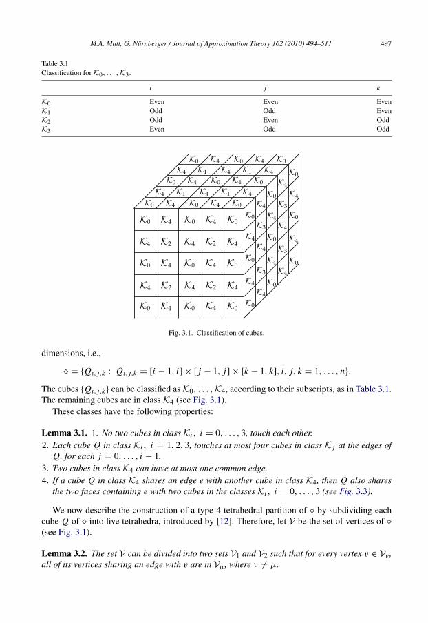
Table 3.1Classification for K0, . . . ,K3.

i j k

K0 Even Even EvenK1 Odd Odd EvenK2 Odd Even OddK3 Even Odd Odd

Fig. 3.1. Classification of cubes.

dimensions, i.e.,

= Qi, j,k : Qi, j,k = [i − 1, i] × [ j − 1, j] × [k − 1, k], i, j, k = 1, . . . , n.

The cubes Qi, j,k can be classified as K0, . . . ,K4, according to their subscripts, as in Table 3.1.The remaining cubes are in class K4 (see Fig. 3.1).

These classes have the following properties:

Lemma 3.1. 1. No two cubes in class Ki , i = 0, . . . , 3, touch each other.2. Each cube Q in class Ki , i = 1, 2, 3, touches at most four cubes in class K j at the edges of

Q, for each j = 0, . . . , i − 1.3. Two cubes in class K4 can have at most one common edge.4. If a cube Q in class K4 shares an edge e with another cube in class K4, then Q also shares

the two faces containing e with two cubes in the classes Ki , i = 0, . . . , 3 (see Fig. 3.3).

We now describe the construction of a type-4 tetrahedral partition of by subdividing eachcube Q of into five tetrahedra, introduced by [12]. Therefore, let V be the set of vertices of (see Fig. 3.1).

Lemma 3.2. The set V can be divided into two sets V1 and V2 such that for every vertex v ∈ Vν ,all of its vertices sharing an edge with v are in Vµ, where ν 6= µ.


This partition of V is not unique in the sense that there can be other partitions of V into V1 andV2 depending on the choice of the vertices.

Without loss of generality we assume that v0,0,0, v0,1,1, v1,0,1, v1,1,0 ∈ V1. Thus all othervertices are uniquely classified and can be more easily described.

We say that the vertices in V1 are of type-1 and those in V2 are of type-2.Now it is possible to define the following type-4 tetrahedral partition:

Definition 3.1 (Type-4 Tetrahedral Partition). Given a cube partition in R3, suppose ∆ is thecollection of tetrahedra which is obtained by splitting each cube Q of into five tetrahedra byconnecting its four type-2 vertices with each other. ∆ is called a type-4 partition of .

For a simpler description of the different tetrahedra in a single cube Qi, j,k we write

T 1i, j,k := 〈vi, j,k, vi, j,k+1, vi, j+1,k, vi+1, j,k〉,

T 2i, j,k := 〈vi, j,k+1, vi, j+1,k, vi, j+1,k+1, vi+1, j+1,k+1〉,

T 3i, j,k := 〈vi, j,k+1, vi+1, j,k, vi+1, j,k+1, vi+1, j+1,k+1〉,

T 4i, j,k := 〈vi, j+1,k, vi+1, j,k, vi+1, j+1,k, vi+1, j+1,k+1〉,

T 5i, j,k := 〈vi, j,k+1, vi, j+1,k, vi+1, j,k, vi+1, j+1,k+1〉,

for the tetrahedra in cubes of the classes K0,K1,K2 and K3 (see Fig. 3.4).For the different tetrahedra in a cube Qi, j,k in class K4 (see Fig. 3.5) we use the notation

T 1i, j,k := 〈vi, j,k, vi, j+1,k, vi, j+1,k+1, vi+1, j+1,k〉,

T 2i, j,k := 〈vi, j,k, vi, j,k+1, vi, j+1,k+1, vi+1, j,k+1〉,

T 3i, j,k := 〈vi, j+1,k, vi+1, j,k+1, vi+1, j+1,k, vi+1, j+1,k+1〉,

T 4i, j,k := 〈vi, j,k, vi+1, j,k, vi+1, j,k+1, vi+1, j+1,k〉,

T 5i, j,k := 〈vi, j,k, vi, j+1,k+1, vi+1, j,k+1, vi+1, j+1,k〉.

4. Partial Worsey–Farin splits

In this section we recall the partial Worsey–Farin split. In order to describe a partialWorsey–Farin split we also need the Clough–Tocher split of a triangle. The Clough–Tocher splitFCT of a triangle F := 〈v1, v2, v3〉 with interior point vF can be obtained by connecting all threevertices of F to vF . Then FCT consists of the three subtriangles Fi := 〈vI , vi+1, vF 〉, i = 1, 2, 3,where v4 = v1.

The following definition can be found in a similar way in [3].

Definition 4.1. Let T be a tetrahedron, and let vT be its barycenter. Given an integer 1 ≤ m ≤ 4,let F1, . . . , Fm be distinct faces of T , and for each i = 1, . . . ,m, let vFi be a point in the interiorof Fi . Then we define the m-th-order partial Worsey–Farin split ∆m

W F of T to be the tetrahedralpartition obtained by the following steps:

1. connect vT to each of the four vertices of T ,2. connect vT to the points vFi for i = 1, . . . ,m,3. connect vFi to the three vertices of Fi for i = 1, . . . ,m.


The m-th-order partial Worsey–Farin split of a tetrahedron results in 4 + 2m subtetrahedra; seeFig. 4.1. The split ∆4

W F is the well-known Worsey–Farin split; see [14]. We need the followingresult on the space S 1

3 (∆mW F ), where ∆m

W F is the m-th-order partial Worsey–Farin split of atetrahedron T := 〈v1, v2, v3, v4〉.

Theorem 4.1 ([3], Theorem 6.3). Fix 0 ≤ m ≤ 4. Let Mm be the union of the following sets ofdomain points in D∆m

W F:

1. for each i = 1, . . . , 4, D(vi ) ∩ Ti for some tetrahedron Ti ∈ ∆mW F containing vi ,

2. for each face F of T that is not split, the point ξ F1,1,1,

3. for each face F of T that has been subjected to a Clough–Tocher split, the points ξ Fi1,1,1

3i=1,

where F1, F2, F3 are the subfaces of F.

Then Mm is a minimal determining set for S 13 (∆

mW F ).

5. Main result

In this section we give an algorithm for the refinement of ∆ to ∆∗ and develop a local andstable Lagrange interpolation method for S 1

3 (∆∗). In this algorithm we split some of the faces

of the tetrahedra with a Clough–Tocher split and the tetrahedra with the corresponding partialWorsey–Farin split. To uniquely define these splits we specify the points vF , where the faceshave to be split, in the following way:

1. if F is a face that is shared by two tetrahedra T and T in ∆, then choose vF to be theintersection of F with the line connecting the barycenters vT and vT of T and T ;

2. otherwise choose the barycenter of F to be vF .

Let be a cube partition and ∆ the corresponding type-4 tetrahedral partition. Moreover, letKi , i = 0, . . . , 4, be the classes of cubes and T l

i, j,k, l = 1, . . . , 5, the tetrahedra as in Section 3.

Algorithm 5.1. Step 1: For each cube Qi, j,k ∈ K0,(1a) choose the 20 points DT 1

i, j,k,

(1b) choose the 10 points DT 2i, j,k\ E

T 2i, j,k

1 (〈vi, j,k+1, vi, j+1,k〉),

(1c) split T 3i, j,k with a first-order partial Worsey–Farin split at 〈vi, j,k+1, vi+1, j,k,

vi+1, j+1,k+1〉 and choose the four points DT1 (vi+1, j,k+1), vi+1, j,k+1 ∈ T ⊂ T 3

i, j,k ,vF ∈ 〈vi+1, j,k, vi+1, j,k+1, vi+1, j+1,k+1〉 and vF ∈ 〈vi, j,k+1, vi+1, j,k, vi+1, j+1,k+1〉,

(1d) and split T 4i, j,k with a first-order partial Worsey–Farin split at 〈vi, j+1,k, vi+1, j,k,

vi+1, j+1,k+1〉 and choose the four points DT1 (vi+1, j+1,k), vi+1, j+1,k ∈ T ⊂ T 4

i, j,k .Step 2: Define all edges of ∆\K0 as “unmarked” and all edges in cubes in class K0 as “marked”.Step 3: For each cube Qi, j,k in Kl , l = 1, . . . , 4, for each tetrahedron T m

i, j,k, m = 1, . . . , 4, inQi, j,k ,3(a) if T := T m

i, j,k has h faces with two or three marked edges, then split these faces witha Clough–Tocher split, T with an h-th-order partial Worsey–Farin split and replaceT in ∆ by the resulting subtetrahedra,

3(b) if a face 〈v1, v2, v3〉 of T has no or two marked edges, choose the point vF ,3(c) mark all edges of T .

Step 4: Split each tetrahedron T 5i, j,k in ∆ with a fourth-order partial Worsey–Farin split.


Table 5.1Possible splits for the different tetrahedra for cubes in K0 ∪ · · · ∪K3.

No split 1-WF 2-WF 3-WF 4-WF

K0T 1i, j,k × – – – –

K0T 2i, j,k × – – – –

K0T 3i, j,k – × – – –

K0T 4i, j,k – × – – –

K0T 5i, j,k – – – – ×

K1T 1i, j,k × – – – –

K1T 2i, j,k – × – – –

K1T 3i, j,k – – × – –

K1T 4i, j,k – – – × –

K1T 5i, j,k – – – – ×

K2T 1i, j,k o × – – –

K2T 2i, j,k – o × – –

K2T 3i, j,k – – o × –

K2T 4i, j,k – – – o ×

K2T 5i, j,k – – – – ×

K3T 1i, j,k o – – × –

K3T 2i, j,k o – – × –

K3T 3i, j,k – – – o ×

K3T 4i, j,k – – – o ×

K3T 5i, j,k – – – – ×

Now, let L be the set of all interpolation points chosen in Algorithm 5.1 and ∆∗ be the tetrahedralpartition obtained from Algorithm 5.1.

It may be helpful to list the types of the splits that may be applied to the tetrahedra in thedifferent classes—see Tables 5.1 and 5.2. m-WF stands for the m-th-order partial Worsey–Farinsplit. In the table the symbol “–” indicates that the corresponding tetrahedra are not subdividedwith the indicated split. The symbol “o” identifies cases which can occur when the correspondingcube is on the boundary of . The splits for tetrahedra of cubes in the interior of are identifiedwith the symbol “×”.

Note that the tetrahedral partition obtained is not the final partition. Let T and T be twotetrahedra with a common face F . By Algorithm 5.1, F has not been split as a face of tetrahedron

T , but it has been split as a face of T . We first determine the spline on T . Then, we split T at Fand represent the spline as a spline on the subdivided tetrahedron T . This representation can beeasily obtained by applying the de Casteljau algorithm. Next, the spline can be determined on T .Note that in the Tables 5.1 and 5.2 these additional splits are not considered.

Definition 5.1. A set L := ξi i=1,...,N is called a Lagrange interpolation set for the spline spaceS 1

3 (∆∗) if N is the dimension of S 1

3 (∆∗) and for every choice of real numbers fi i=1,...,N there

is a unique spline s ∈ S satisfying

s(ξi ) = fi , i = 1, . . . , N .


Table 5.2Possible splits for the different tetrahedra for cubes in K4.

No split 1-WF 2-WF 3-WF 4-WF

K4T 1i, j,k – o – – ×

K4T 2i, j,k – o o – ×

K4T 3i, j,k – – – o ×

K4T 4i, j,k – – – – ×

K4T 5i, j,k – – – – ×

Fig. 3.2. Layers of cubes.

Definition 5.2. A Lagrange interpolation set L is local if for any tetrahedron T in ∆∗ and aspline s ∈ S 1

3 (∆∗), s|T depends only on values fξ ξ∈L∩ΩT , with ΩT ⊂ Ω .

L is also stable if

|cξ | ≤ K maxη∈ΩT

| fη| (5.1)

holds for the B-coefficients cξ of s|T , with an absolute constant K .

Now, we are ready to state the main result of this paper.

Theorem 5.1. L is a local and stable Lagrange interpolation set for S13(∆

∗).

Before giving the proof, we describe how a spline on can be computed. Therefore, we arguewith layers of cubes; see Fig. 3.2. In Algorithm 5.1, we first choose the interpolation points intetrahedra of cubes in class K0. These can be chosen independently, since the cubes in class K0are disjoint (cf. Lemma 3.1). Thus, we can compute s on all cubes in class K0 independently.Moreover, for all cubes in class K0, these computations are the same.

Next, s can be computed on the cubes in class K1. Therefore, the interpolation points intetrahedra of cubes in class K1 are chosen considering the common edges with cubes in K0. Thecomputations are very similar to those for the cubes in class K0. For cubes in class K1 in theinterior of , we always have the same computations, since these cubes are disjoint and each onetouches exactly four cubes in class K0, which lie in the same layer. Thus, s only depends on thevalues of the interpolation points in each cube in class K1 and at most four cubes in class K0 witha common edge in the same layer. In the same way s can be computed in the cubes in the otherclasses. So we compute s in the cubes of K0,K1,K2,K3 and finally K4 (see Figs. 3.4 and 3.5).


Fig. 3.3. Cube Q ∈ K4 sharing e with a cube in class K4 and sharing two faces with cubes in classes Ki andK j , i, j = 0, . . . , 3.

Fig. 3.4. The partition of a cube Qi, j,k ∈ K0 ∪K1 ∪K2 ∪K3 into five tetrahedra with marked vertices of type-1 andtype-2.

Therefore, a spline s can be computed locally in the sense that s|Q , where Q is a cube in classK4, only depends on values in Q and the coefficients of s in the surrounding cubes.

For the proof of our main result we need the following two bivariate Lemmas from [3].Therefore, we also need some bivariate Bernstein–Bezier techniques (cf. [5], chapter 2.3). LetD F := ξ

Ti, j,k :=

iv1+ jv2+kv33 , i + j + k = 3 be the set of domain points of a triangle F :=

〈v1, v2, v3〉. Moreover, let Bi, j,ki+ j+k=3 be the bivariate Bernstein polynomials associated withF . Then every bivariate polynomial p of degree 3 can be uniquely written as

p =∑

i+ j+k=3

cFi, j,k Bi, j,k,

where cFi, j,k are the B-coefficients of p associated with the domain points in F .

Lemma 5.1. Suppose that we are given all of the coefficients cFi, j,k of a bivariate cubic

polynomial p except for cF1,1,1. Then for any given real number z and any point vF in the interior

of F, there exists a unique cF1,1,1 such that p(vF ) = z.

Let FCT be a triangle which has been subjected to the Clough–Tocher split with subfacesFi , i = 1, 2, 3, as in Section 4. Moreover, let s be a bivariate cubic C1 spline, with B-coefficientscFl

i, j,ki+ j+k=3,l=1,2,3.


Fig. 3.5. The partition of a cube Qi, j,k ∈ K4 into five tetrahedra with marked vertices of type-1 and type-2.

Fig. 4.1. Partial Worsey–Farin splits of m-th order for m = 1, . . . , 4.

Lemma 5.2. Suppose that we are given all of the coefficients of s ∈ S13(FCT ) except for

cF13,0,0, cF1

2,1,0, cF12,0,1, cF1

1,1,1. Then for any given real number z, there exists a unique choice of thesecoefficients such that s(vF ) = z.

Note that the spline in Lemma 5.2 is not uniquely determined without the interpolation conditionat vF .

Proof of Theorem 5.1. To show that L is a local Lagrange interpolation set for S13(∆

∗), we fixthe values zξ ξ∈L for a spline s ∈ S1

3(∆∗). Then we show that s is locally, stably and uniquely

determined. We have to consider three cases.Case 1: Qi, j,k ∈ K0.

We begin with s|Qi, j,k , Qi, j,k ∈ K0. By Lemma 3.1 all cubes Qi, j,k ∈ K0 are disjoint.Therefore, we only consider one cube Q ∈ K0; the remaining cubes in class K0 can be treatedanalogously. For simplicity, in the following we set i = j = k = 0.


Case 1.1: T 10,0,0.

Since L contains all the points DT 10,0,0

, the B-coefficients of s|T 10,0,0

can be uniquely and stably

computed form the values zξ ξ∈L∩T 10,0,0

. Thus, all B-coefficients of s associated with domain

points in D1(v), v ∈ T 10,0,0, and E1(e), e ∈ T 1

0,0,0, can be uniquely and stably determined using

the C1 smoothness conditions of s at the edges and vertices of T 10,0,0. Since these computations

only involve values zξ ξ∈L∩T 10,0,0

, they are also local.

Case 1.2: T 20,0,0.

Next, we consider the tetrahedron T 20,0,0. The B-coefficients associated with the 10

domain points in ET 2

0,0,01 (〈v0,0,1, v0,1,0〉) are already uniquely determined. Then the remaining

undetermined B-coefficients of s|T 20,0,0

can be uniquely and stably computed using the values

zξ ξ∈L∩T 20,0,0

. Thus, the spline s|T 20,0,0

can be computed locally, since the corresponding B-

coefficients only depend on the values zξ ξ∈L∩(T 10,0,0∪T 2

0,0,0). Now, also all B-coefficients of s

associated with domain points in D1(v), v ∈ T 20,0,0, and E1(e), e ∈ T 2

0,0,0, can be uniquely and

stably determined using the C1 smoothness conditions of s at the edges and vertices of T 20,0,0.

Case 1.3: T 30,0,0.

Next, we consider the tetrahedron T 30,0,0, which has been subjected to a first-order partial

Worsey–Farin split. The B-coefficients associated with the domain points in E1(〈v0,0,1, v1,0,0〉)∪

E1(〈v0,0,1, v1,1,1〉) are already uniquely determined. Those coefficients associated with thedomain points in D1(v1,0,1) can be uniquely determined from the values at the interpolationpoints ξ ∈ DT

1 (v1,0,1) ⊂ L, v1,0,1 ∈ T ⊂ T 30,0,0. The undetermined B-coefficients in the

faces 〈v1,0,0, v1,0,1, v1,1,1〉 and 〈v0,0,1, v1,0,0, v1,1,1〉 can be computed from the values at thetwo points vF ∈ L and vF ∈ L in these faces using Lemmas 5.1 and 5.2, respectively. Thus,all B-coefficients associated with the domain points in the minimal determining set M1 fromTheorem 4.1 are uniquely and stably determined. Therefore, all other B-coefficients of s|T 3

0,0,0

are uniquely and stably determined. The computation of these B-coefficients is also local, sincethey only depend on the values zξ ξ∈L∩(T 1

0,0,0∪T 20,0,0∪T 3

0,0,0). So, all B-coefficients of s associated

with domain points in D1(v), v ∈ T 30,0,0, and E1(e), e ∈ T 3

0,0,0, can be uniquely and stably

determined using the C1 smoothness conditions of s at the edges and vertices of T 30,0,0.

Case 1.4: T 40,0,0.

Now, we consider the tetrahedron T 40,0,0. This tetrahedron has also been subjected to a

first-order partial Worsey–Farin split. Moreover, the B-coefficients associated with the domainpoints in E1(〈v0,1,0, v1,0,0〉) ∪ E1(〈v0,1,0, v1,1,1〉) ∪ E1(〈v1,0,0, v1,1,1〉) are already uniquelydetermined. Thus, all B-coefficients of s|〈v0,1,0,v1,0,0,v1,1,1〉 are already uniquely and stablydetermined, since we already know the B-coefficients corresponding to the domain points in theminimal determining set of the classical Clough–Tocher macro-element (cf. [1]). The remainingB-coefficients of s|T 4

0,0,0can be uniquely and stably determined from the values at the

interpolation points ξ ∈ DT1 (v1,1,0) ⊂ L, v1,1,0 ∈ T ⊂ T 4

0,0,0. Thus, all B-coefficients of s

associated with domain points in D1(v), v ∈ T 40,0,0, and E1(e), e ∈ T 4

0,0,0, can be uniquely and

stably determined using the C1 smoothness conditions of s at the edges and vertices of T 40,0,0.

At this point s is uniquely and stably determined on all edges of ∆∗.


Case 1.5: T 50,0,0.

Next, we consider the last tetrahedron in Q, T 50,0,0. By the construction of ∆, T 5

0,0,0 has

one common face with each of the four tetrahedra T l0,0,0, l = 1, . . . , 4. Furthermore, by

Algorithm 5.1 T 50,0,0 has been subjected to the fourth-order partial Worsey–Farin split. Since

s|T l0,0,0, l = 1, . . . , 4, is already uniquely determined, we use the de Casteljau Algorithm to

subdivide the tetrahedra T l0,0,0, l = 1, 2, 3, with a partial Worsey–Farin split with a split face

at the common face with T 50,0,0 and the C1 smoothness conditions at the edges and vertices of

∆∗, to uniquely and stably determine the B-coefficients associated with the domain points on thefaces of T 5

0,0,0. Now, we have determined all B-coefficients associated with the domain points inthe minimal determining set M4 for a spline s over the fourth-order partial Worsey–Farin splitand the remaining undetermined B-coefficients of s|T 5

0,0,0can be uniquely and stably computed

(see Theorem 4.1). These computations are also local, since the B-coefficients of s|T 50,0,0

only

depend on the values zξ ξ∈L∩Q .Case 2: Qi, j,k ∈ (K1 ∪K2 ∪K3).

In the following we consider the cubes Qi, j,k ∈ (K1 ∪ K2 ∪ K3). The spline s is determinedon these cubes according to the ordering imposed by their classes. So, first s can be determinedon all cubes in the class K1, then on all cubes in class K2 and afterwards on all cubes in classK3. By Lemma 3.1, no two cubes in class Ki , i = 0, . . . , 3, touch each other. Therefore, wecan compute s on each cube Qi, j,k ∈ Kl , l = 1, . . . , 3, in the same way. These computationsare also very similar to those for determining s|K0 . Let Q be a cube in (K1 ∪ K2 ∪ K3) andT l

i, j,k, l = 1, . . . , 5, the tetrahedra in Q. Since s is already uniquely determined on the edges of∆∗, the only undetermined B-coefficients of s|Q are associated with domain points on the faces

of the tetrahedra in Q.Case 2.1: T 1

i, j,k, T 2i, j,k, T 3

i, j,k, T 4i, j,k .

We first consider the faces of the tetrahedron T 1i, j,k . Let F be a face of T 1

i, j,k . We have todistinguish four cases:

(1) If F has no marked edges, then L contains the barycenter vF of F and the remainingundetermined B-coefficient of s|F can be uniquely and stably determined using Lemma 5.1.

(2) If F has one marked edge, then the remaining undetermined B-coefficient of s|F can beuniquely and stably determined using the C1 smoothness conditions at the marked edge.

(3) If F has two marked edges, then F is split with a Clough–Tocher split and L contains thebarycenter vF of F and the remaining undetermined B-coefficients of s|F can be uniquelyand stably determined using Lemma 5.2.

(4) If F has three marked edges, then F is split with a Clough–Tocher split and the remainingundetermined B-coefficients of s|F can be uniquely and stably computed using the C1

smoothness conditions at the edges of F , since s|F is just a classical C1 Clough–Tochermacro-element (cf. [1]).

If none of the faces of T 1i, j,k is subdivided by a Clough–Tocher split, s|T 1

i, j,kis uniquely and

stably determined. If one or more of the faces of T 1i, j,k is subdivided, we can use Theorem 4.1 to

uniquely and stably determine s|T 1i, j,k

. All these computations are also local. The spline s|T 1i, j,k

can be uniquely determined from values corresponding to interpolation points in T 1i, j,k , the

B-coefficients of s associated with domain points in the cubes in class K0 sharing vertices withQ and the maximal four cubes in class Ki−1 touching Q at the edges, where Q is in class Ki .The cube Q can touch fewer cubes in class Ki−1 if it lies on the boundary of .


On the tetrahedra T li, j,k, l = 2, 3, 4, s can be determined in the same way as on T 1

i, j,k . Theonly difference is, that s|T l

i, j,k, l = 2, 3, 4, then also depends on the B-coefficients of s associated

with domain points in the tetrahedra T mi, j,k, m = 1, . . . , l.

Case 2.2: T 5i, j,k .

Now, we can determine s|T 5i, j,k

. The tetrahedron T 5i, j,k has exactly one common face with each

of the four tetrahedra T 1i, j,k, . . . , T 4

i, j,k and by Algorithm 5.1 T 5i, j,k has been subjected to the

fourth order partial Worsey–Farin split. So, we use the de Casteljau Algorithm to subdivide thetetrahedra T 1

i, j,k, . . . , T 4i, j,k with a partial Worsey–Farin split with a split face at the common face

with T 5i, j,k , if not done earlier, and the C1 smoothness conditions at the edges and vertices of ∆∗,

to uniquely and stably determine the B-coefficients associated with the domain points on the facesof T 5

i, j,k . Thus, we have determined all B-coefficients associated with the domain points in theminimal determining set M4 for a spline s over the fourth-order partial Worsey–Farin split andthe remaining undetermined B-coefficients of s|T 5

i, j,kcan be uniquely and stably computed (see

Theorem 4.1). These computations are also local, since the B-coefficients of s|T 5i, j,k

depend on the

same values and already determined B-coefficients as the previous tetrahedra T 1i, j,k, . . . , T 4

i, j,k .Case 3: Qi, j,k ∈ K4.

Finally, we determine s|Qi, j,k , Qi, j,k ∈ K4. Let Q be a cube in class K4. Then the tetrahedra

in Q can be determined in the same way and in the same ordering as the tetrahedra in the cubesin K0, . . . ,K3. Note that for each tetrahedron T sharing a face with a tetrahedron T ∈ Q we alsosplit these faces in the neighboring tetrahedra, if this has not already happened, and use the deCasteljau Algorithm to subdivide s|T with the corresponding partial Worsey–Farin split.

These computations are also local and stable and s|Q depends only on the values associated

with the interpolation points inside Q and the B-coefficients of s associated with the domainpoints in the cubes sharing an edge or a vertex with Q, which are not in K4. Moreover, none ofthe C1 smoothness conditions is violated. By Lemma 3.1 two cubes in class K4 can only touchon edges and moreover Q must also touch two cubes in the classes Ki , i = 0, . . . , 3, at theseedges. But s is already determined on the cubes in these classes.

In the proof it is shown that L is a local and stable Lagrange interpolation method for S 13 (∆

∗).Since the spline is computed locally on each cube, it can easily be seen that for any tetrahedronT of a cube in class K4, s|T depends only on values zξ ξ∈L∩ΩT , where ΩT is the collectionof at most 5 × 5 × 7 cubes, where T lies in the middle of ΩT . But we emphasize that s onlydepends on the cubes in ΩT of lower class. Thus, for tetrahedra in cubes of lower class, ΩT isstill smaller. Moreover, since we only use the C1 smoothness conditions and some small systemsof linear equations to determine s, all computations needed to uniquely determine s are stable inthe sense that

|cξ | ≤ maxη∈ΩT

|zη| (5.2)

holds with an absolute constant K , since the angles of ∆ are bounded away from zero by anabsolute constant independent of the mesh size of ∆. Therefore, also

‖s‖T ≤ K‖ f ‖ΩT (5.3)

holds with an absolute constant K , where s is the interpolating spline of the function f ∈ C(Ω).


Remark 5.1. In the notation of [5], L and S 13 (∆

∗) form a Lagrange interpolation pair. Moreover,from the proof of Theorem 5.1 it is easy to see that L is a minimal determining set for S 1

3 (∆∗)

and that the set εξ ξ∈L is also a nodal minimal determining set for S 13 (∆

∗), where εξ denotesthe point evaluation at the point ξ in Ω .

6. Bounds on the error of the interpolant

In this section we want to provide a bound on the error ‖ f − s‖Ω for smooth functions, wherethe error is measured in the maximum norm on Ω .

Let L be the Lagrange interpolation method constructed in Section 5 associated with the splinespace S 1

3 (∆∗). Then for every f ∈ C(Ω), there is a unique spline I f ∈ S 1

3 (∆∗) such that

I f (ξ) = f (ξ), ξ ∈ L. (6.1)

This defines a linear projector I mapping C(Ω) onto S 13 (∆

∗).Now for a compact set B ⊆ Ω and an integer m ≥ 1, let W m

∞(B) be the usual Sobolev spacedefined on B with seminorm

| f |m,B :=∑|α|=m

‖Dα f ‖B,

where ‖ · ‖B denotes the infinity norm on B and Dα:= Dα1

x Dα2y Dα3

z with α = (α1, α2, α3). Let|∆∗| be the mesh size of ∆∗, i.e. the maximum diameter of the tetrahedra in ∆∗.

Theorem 6.1. Let f ∈ W m+1∞ (Ω) for some 0 ≤ m ≤ 3. Then there exists an absolute constant

K such that

‖Dα( f − I f )‖Ω ≤ K |∆∗|m+1−|α|| f |m+1,Ω , (6.2)

for all multi-indices α with 0 ≤ |α| ≤ m.

Proof. Fix m, and let f ∈ W m+1∞ (Ω). Fix T ∈ ∆∗, and let ΩT be as in Section 5. By Lemma

4.3.8 of [2], there exists a cubic polynomial p such that

‖Dβ( f − p)‖ΩT ≤ K2|ΩT |m+1−|β|

| f |m+1,ΩT , (6.3)

for all 0 ≤ |β| ≤ m, where |ΩT | is the diameter of ΩT . Since I p = p, it follows that

‖Dα( f − I f )‖T ≤ ‖Dα( f − p)‖T + ‖D

αI( f − p)‖T .

Due to (6.3) with β = α, it suffices to estimate the second term ‖DαI( f − p)‖T . By the Markovinequality [13] and (5.3)

‖DαI( f − p)‖T ≤ K3|T |−|α|‖I( f − p)‖T ≤ K4|T |

−|α|‖ f − p‖ΩT ,

where |T | is the diameter of T . Because of the geometry of the partition, two absolute constantsK5 and K6 exist with ΩT ≤ K5|T | and |T | ≤ K6|∆∗|. In view of this and by inserting (6.3) withβ = 0 for ‖ f − p‖ΩT , we get

‖Dα( f − I f )‖T ≤ K1|ΩT |m+1−|α|

| f |m+1,ΩT .

Now taking the maximum over all tetrahedra in ∆∗ leads to (6.2).

Thus, it is also shown that the Lagrange interpolation method constructed in this paper yieldsoptimal approximation order.


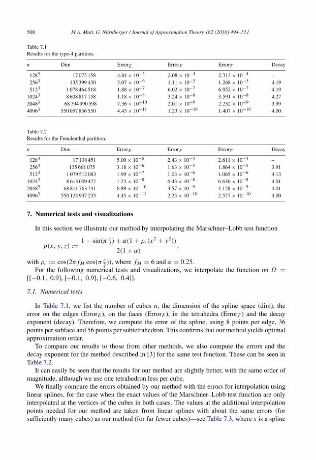
Table 7.1Results for the type-4 partition.

n Dim ErrorE ErrorF ErrorT Decay

1283 17 073 158 4.84× 10−5 2.08× 10−4 2.313× 10−4 –2563 135 399 430 3.07× 10−6 1.11× 10−5 1.268× 10−5 4.195123 1 078 464 518 1.88× 10−7 6.02× 10−7 6.952× 10−7 4.19

10243 8 608 817 158 1.18× 10−8 3.24× 10−8 3.591× 10−8 4.2720483 68 794 990 598 7.36× 10−10 2.01× 10−9 2.252× 10−9 3.9940963 550 057 836 550 4.43× 10−11 1.23× 10−10 1.407× 10−10 4.00

Table 7.2Results for the Freudenthal partition.

n Dim ErrorE ErrorF ErrorT Decay

1283 17 138 451 5.00× 10−5 2.43× 10−4 2.811× 10−4 –2563 135 661 075 3.18× 10−6 1.63× 10−5 1.864× 10−5 3.915123 1 079 512 083 1.99× 10−7 1.03× 10−6 1.065× 10−6 4.13

10243 8 613 009 427 1.23× 10−8 6.43× 10−8 6.630× 10−8 4.0120483 68 811 763 731 6.89× 10−10 3.57× 10−9 4.128× 10−9 4.0140963 550 124 937 235 4.45× 10−11 2.23× 10−10 2.577× 10−10 4.00

7. Numerical tests and visualizations

In this section we illustrate our method by interpolating the Marschner–Lobb test function

p(x, y, z) :=1− sin(π z

2 )+ α(1+ ρr (x2+ y2))

2(1+ α),

with ρr := cos(2π fM cos(π r2 )), where fM = 6 and α = 0.25.

For the following numerical tests and visualizations, we interpolate the function on Ω =[[−0.1, 0.9], [−0.1, 0.9], [−0.6, 0.4]].

7.1. Numerical tests

In Table 7.1, we list the number of cubes n, the dimension of the spline space (dim), theerror on the edges (ErrorE ), on the faces (ErrorF ), in the tetrahedra (ErrorT ) and the decayexponent (decay). Therefore, we compute the error of the spline, using 8 points per edge, 36points per subface and 56 points per subtetrahedron. This confirms that our method yields optimalapproximation order.

To compare our results to those from other methods, we also compute the errors and thedecay exponent for the method described in [3] for the same test function. These can be seen inTable 7.2.

It can easily be seen that the results for our method are slightly better, with the same order ofmagnitude, although we use one tetrahedron less per cube.

We finally compare the errors obtained by our method with the errors for interpolation usinglinear splines, for the case when the exact values of the Marschner–Lobb test function are onlyinterpolated at the vertices of the cubes in both cases. The values at the additional interpolationpoints needed for our method are taken from linear splines with about the same errors (forsufficiently many cubes) as our method (for far fewer cubes)—see Table 7.3, where s is a spline


Table 7.3Results for a spline from linear data.

n Error s N Error slin n Error s

2563 1.2678× 10−5 56323 2.72× 10−6 2563 3.57× 10−5

3603 3.86× 10−6 100803 8.39× 10−7 3603 4.15× 10−6

5123 6.95× 10−7 225283 1.67× 10−7 5123 7.98× 10−7

Table 7.4Data reduction for linear splines.

n Dimension cubic spline N Dimension linear spline Quotient

2563 135 399 430 16003 4 096 000 000 30.253603 375 583 686 46003 97 336 000 000 259.165123 1 078 464 518 108003 1 259 712 000 000 1168.06

Fig. 7.1. Isosurface with value 0.5 of the Marschner–Lobb test function with 200× 200× 200 cubes, visualized by ourmethod.

constructed from exact data at all Lagrange interpolation points, slin a linear spline and s a splinewith exact data only at the vertices of the cubes. Moreover, n is the number of cubes for the cubicsplines and N the number of cubes for the linear splines.

The results show that if we compare the dimensions of the space of cubic C1 splines used forour method with the dimensions of the spaces of linear splines which yield approximately thesame errors, we obtain data reductions up to factor 103—see Table 7.4, where n is the number ofcubes for the cubic splines and N the number of cubes for the linear splines. Moreover, we alsolist the quotient of the dimension of the linear spline and the cubic spline.

7.2. Visualizations

In the following we also illustrate the application of our method. Therefore, we visualize anisosurface with value 0.5 of the Marschner–Lobb test function with 200× 200× 200 cubes. Toshow the smoothness of the interpolant more clearly, we also visualize an enlargement of a smallsection of the isosurfaces (see Fig. 7.1).


Fig. 7.2. Isosurface with value 0.5 of the Marschner–Lobb test function with 200× 200× 200 cubes, visualized by themethod described in [3].

In order to compare the results visually, we also illustrate the method described in [3] (seeFig. 7.2).

Acknowledgments

We would like to thank Georg Schneider for performing the numerical tests and constructingthe visualizations.

References

[1] P. Alfeld, L.L. Schumaker, Smooth macro-elements based on Clough–Tocher triangle splits, Numer. Math. 90(2002) 597–616.

[2] S.C. Brenner, L.R. Scott, The Mathematical Theory of Finite Element Methods, in: Texts in Applied Mathematics,vol. 15, Springer-Verlag, New York, 1994.

[3] G. Hecklin, G. Nurnberger, L.L. Schumaker, F. Zeilfelder, A local Lagrange interpolation method based on C1

cubic splines on Freudenthal partitions, Math. Comp. 77 (2008) 1017–1036.[4] G. Hecklin, G. Nurnberger, L.L. Schumaker, F. Zeilfelder, Local Lagrange interpolation with cubic C1 splines on

tetrahedral partitions, J. Approx. Theory, 2008, in press (doi:10.1016/j.jat.2008.01.012).[5] M.-J. Lai, L.L. Schumaker, Spline Functions on Triangulations, Cambridge University Press, 2007.[6] G. Nurnberger, F. Zeilfelder, Local Lagrange interpolation by cubic splines on a class of triangulations,

in: K. Kopotun, T. Lyche, M. Neamtu (Eds.), Trends in Approximation Theory, Vanderbilt University Press,Nashville, TN, 2001, pp. 341–350.

[7] G. Nurnberger, F. Zeilfelder, Lagrange interpolation by bivariate C1-splines with optimal approximation order,Adv. Comput. Math. 21 (2004) 381–419.

[8] G. Nurnberger, V. Rayevskaya, L.L. Schumaker, F. Zeilfelder, Local Lagrange interpolation with C2-splines ofdegree seven on triangulations, in: M. Neamtu, E. Saff (Eds.), Advances in Constructive Approximation, Vanderbilt2003, Nashboro Press, Brentwood, TN, 2004, pp. 345–370.

[9] G. Nurnberger, L.L. Schumaker, F. Zeilfelder, Lagrange interpolation by C1 cubic splines on triangulatedquadrangulations, Adv. Comput. Math. 21 (3–4) (2004) 357–380.

[10] G. Nurnberger, L.L. Schumaker, F. Zeilfelder, Two Lagrange interpolation methods based on C1 splines ontetrahedral partitions, in: C. Chui, M. Neamtu, L.L. Schumaker (Eds.), Approximation Theory XI: Gatlinburg 2004,Nashboro Press, Brentwood, TN, 2005, pp. 327–344.

[11] G. Nurnberger, V. Rayevskaya, L.L. Schumaker, F. Zeilfelder, Local Lagrange interpolation with bivariate splinesof arbitrary smoothness, Constr. Approx. 23 (2006) 33–59.

http://dx.doi.org/doi:10.1016/j.jat.2008.01.012


[12] L.L. Schumaker, T. Sorokina, C1 quintic splines on type-4 tetrahedral partitions, Adv. Comput. Math. 21 (3–4)(2004) 421–444.

[13] D.R. Wilhelmsen, A Markov inequality in several dimensions, J. Approx. Theory 11 (3) (1974) 216–220.[14] A.J. Worsey, G. Farin, An n-dimensional Clough–Tocher interpolant, Constr. Approx. 3 (1) (1987) 99–110.

Documents

Local Lagrange interpolation using cubic C1 splines on ... · M.A. Matt, G. Nurnberger / Journal of Approximation Theory 162 (2010) 494–511¨ 495 In this paper, we describe a local