Local GMM Estimation of Time Series Models withConditional Moment Restrictions�

Nikolay Gospodinovy

Concordia University and CIREQTaisuke Otsuz

Yale University

First Version: September 2008Revised: December 2009

AbstractThis paper investigates statistical properties of the local generalized method of moments (LGMM)estimator for some time series models de�ned by conditional moment restrictions. First, weconsider Markov processes with possible conditional heteroskedasticity of unknown forms andestablish the consistency, asymptotic normality, and semi-parametric e¢ ciency of the LGMMestimator. Second, we undertake a higher-order asymptotic expansion and demonstrate thatthe LGMM estimator possesses some appealing bias reduction properties for positively autocor-related processes. Our analysis of the asymptotic expansion of the LGMM estimator reveals aninteresting contrast with the OLS estimator that helps to shed light on the nature of the biascorrection performed by the LGMM estimator. The practical importance of these �ndings isevaluated in terms of a bond and option pricing exercise based on a di¤usion model for spotinterest rate.

Keywords: Conditional moment restriction; Local GMM; Higher-order expansion; Conditionalheteroskedasticity.

JEL Classification: C13; C22; G12.

�We would like to thank the editors, a co-editor, three anonymous referees, conference participants at the 2007CIREQ conference on Generalized Method of Moments, the 2007 meeting of the Canadian Econometrics Study Groupand the 2009 Joint Statistical Meetings for useful comments and suggestions. Financial support from FQRSC andSSHRC (Gospodinov) and National Science Foundation under SES-0720961 (Otsu) is gratefully acknowledged.

yCorresponding author: Department of Economics, Concordia University, 1455 de Maisonneuve Blvd. West,Montreal, Quebec, H3G 1M8 Canada, email: nikolay.gospodinov@concordia.ca.

zCowles Foundation and Department of Economics, Yale University, P.O. Box 208281, New Haven, CT, 06520-8281USA, email: taisuke.otsu@yale.edu.

1 Introduction

While modern economic theory typically implies a set of conditional moment restrictions, estimation

of the model parameters is often performed using a framework based on unconditional moment

restrictions such as the standard generalized method of moments (GMM). Despite its computational

attractiveness, this GMM-based approach may result in e¢ ciency losses and inconsistency that

arises from possible nonidenti�ability of the parameters of interest by the unconditional moment

restrictions even when the conditional moment restrictions identify the parameters (Dominguez

and Lobato, 2004). Time series regression models, for example, are usually de�ned in terms of a

sequence of disturbances whose expectation conditional on a few recent lags of the data is assumed

to be zero. This speci�cation allows for conditional heteroskedasticity which is a stylized feature of

many economic and �nancial time series data such as interest rates, exchange rates, asset returns,

etc.

This paper studies estimation of conditional moment restriction models in a time series context.

In particular, we focus on the local (conditional or smoothed) GMM (LGMM, hereafter) estimator

that belongs to the class of localized versions of the generalized empirical likelihood estimator

(Newey and Smith, 2004) introduced and developed by Kitamura, Tripathi and Ahn (2004), Smith

(2007), and Antoine, Bonnal and Renault (2007) (see, e.g., Newey, 1990, 1993; Carrasco and

Florens, 2000; and Donald, Imbens and Newey, 2003, for some alternative methods to estimate

conditional moment restriction models). While all these papers investigate the properties of the

local estimators for iid data, we study the �rst- and higher-order asymptotic properties of the

LGMM estimator for strictly stationary and geometrically ergodic Markov processes.

First, we study the �rst-order asymptotic behavior of the LGMM estimator and show that the

LGMM estimator is consistent and asymptotically normal, and attains the semi-parametric e¢ -

ciency bound for conditional moment restrictions with a martingale di¤erence structure derived in

Carrasco and Florens (2004). We should note that semi-parametrically e¢ cient moment-based esti-

mators have been proposed by Carrasco, Chernov, Florens and Ghysels (2007), Kuersteiner (2001,

2002) and West, Wong and Anatolyev (2009) for more general time series processes. Although

our Markov setup is more restrictive than the setups of these papers, our emphasis is on the bias

property of the LGMM estimator in small samples and the Markov setup helps us to simplify the

higher-order analysis of the estimator. Indeed, our simulation results for AR models with condi-

tional heteroskedasticity suggest that the LGMM estimator is characterized by a smaller bias and

mean squared error than these alternative estimators and, in some cases, even the infeasible GLS

estimator.

Next, in order to explain the bias reduction property of the LGMM estimator, we consider

1

explicitly the AR(1) model with iid errors and undertake a higher-order expansion for the LGMM

estimator. In particular, while the bias of the OLS estimator is given by a single negative term

of order O(T�1), the higher-order expansion of the LGMM estimator reveals the presence of two

O(T�1) bias terms. We compare these terms with those of the OLS estimator and provide an

approximation formula for one of them. Our numerical results show that for positively autocorre-

lated processes the two leading bias terms in the LGMM estimator tend to have opposite signs and

similar magnitudes that o¤set each other. Also, this bias reduction is achieved without in�ating

the variance of the LGMM estimator and then the LGMM can potentially dominate the GLS and

other e¢ cient estimators in terms of mean squared errors. The economic signi�cance of the bias

reduction property of the LGMM estimator is assessed for derivative interest rate products whose

prices exhibit strong sensitivity to the parameter that governs the persistence of the process. In-

terestingly, the LGMM estimator seems to outperform in terms of mean square error the infeasible

optimal GMM as the LGMM tends to remove a substantial portion of the bias that arises from the

highly persistent dynamics of the interest rate data.

Our paper complements the existing econometric and statistical literature which is concerned

with extending the local estimators for moment condition models to dependent data. For example,

Kitamura (1997) considers unconditional moment restrictions with weakly dependent data and

proposes a non-local empirical likelihood estimator by using blocked (or local average) moment

restrictions. Our paper has three important di¤erences with Kitamura (1997): (i) while Kitamura

(1997) focuses on unconditional moments, we consider conditional moment restrictions that imply

an in�nite number of unconditional moments, (ii) while Kitamura (1997) requires local averaging

for moments to account for the long-run variance of the unconditional sample moments, we employ

local averaging to nonparametrically approximate the conditional moment restrictions, and (iii)

while Kitamura (1997) allows for general weakly dependent data, our analysis is restricted to

Markov processes.

In a di¤erent but related strand of literature, Chen, Härdle and Li (2003) propose a goodness-of-

�t test statistic based on the local empirical likelihood function to check the validity of conditional

moment restrictions. Furthermore, Su and White (2003) adopt the local empirical likelihood frame-

work to test conditional independence restrictions which imply sequences of conditional moment

restrictions. Both papers focus on hypothesis testing with possibly dependent data and derive �rst-

order asymptotic properties of the local empirical likelihood-based test statistics. In contrast, we

focus on point estimation of parameters in conditional moment restriction models and derive some

�rst- and higher-order properties of the LGMM estimator. Finally, Gagliardini, Gourieroux and

Renault (2007) extend the local estimation approach to estimate conditional moments of interest

(derivative prices in their example) with dependent data when the conditional moment restrictions

2

(say, E[u1(yt+1; �0)jxt] = 0) and local moment restrictions (say, E[u2(yt+1; �0)jxt = �x] = 0 for somegiven �x) coexist. While Gagliardini, Gourieroux and Renault (2007) use the LGMM approach to

evaluate the local moments E[u2(yt+1; �0)jxt = �x] = 0, they adopt the optimal instrumental variableapproach of Chamberlain (1987) and Newey (1990, 1993) to accommodate the conditional moments

E[u1(yt+1; �0)jxt] = 0. Our setup di¤ers from Gagliardini, Gourieroux and Renault (2007) since

we do not consider the local moments E[u2(yt+1; �0)jxt = �x] = 0 but utilize the LGMM framework

to estimate the parameters �0 in the conditional moments E[u1(yt+1; �0)jxt] = 0. Also, the generaltheoretical arguments in Gagliardini, Gourieroux and Renault (2007) are mostly concerned with

deriving the e¢ ciency bounds in their setup. On the other hand, we are interested in establishing

the �rst- and higher-order asymptotic properties of the LGMM estimator.

The rest of the paper is organized as follows. The next section describes the model and esti-

mation procedure. Section 3 develops the �rst-order asymptotic theory for the LGMM estimator

and reports some numerical properties of the estimator in �nite samples. Section 4 derives the

higher-order asymptotic expansion of the LGMM estimator in an AR(1) model with iid errors and

analyzes the bias properties of the estimator. The bias terms of the LGMM and OLS estimators

are evaluated by simulation. Section 5 assesses the economic signi�cance of the bias reduction and

the e¢ ciency of the LGMM in the context of a bond and derivative pricing exercise. Section 6

concludes. All proofs are contained in the appendix.

2 Model and Estimation Procedure

Suppose that the univariate process of interest frtg1t=�1 on R is strictly stationary and geometri-cally ergodic1 and denote the conditional moment restrictions imposed by some economic theory

as

E [u (rt+1; rt; : : : ; rt�p+1; �0) jrt; : : : ; rt�p+1] = 0; (1)

for each t 2 Z = f: : : ;�1; 0; 1; : : :g, where u : Rp+1 ��! Rl is a known function up to a vector ofunknown parameters �0 2 � � Rk. Technical conditions that restrict the dependence structure ofthe process and ensure the validity of the estimation procedure are discussed in the next section.

One popular example of this framework is the AR(1) model with martingale di¤erence errors

rt+1 = 0 + 1rt + ut+1; E [ut+1jrt] = 0; (2)

1Let fXtg1t=�1 be a time-homogeneous Markov process with state space (Rp;B (Rp)), where B (Rp) is a Borel�-algebra of Rp, and m-step transition probability Pm (x;A) = P (Xm 2 AjX0 = x) for x 2 A and A 2 B (Rp).The process fXtg1t=�1 is geometrically ergodic if there exists a probability measure � on (Rp;B (Rp)), a constant0 < � < 1, and a �-integrable non-negative measurable function C (�) such that kPm (x; �)� � (�)k� � �mC (x) forall m 2 N and x 2 Rp, where k�k� denotes the total variation norm (Carrasco and Chen, 2002; Meyn and Tweedie,1993).

3

for each t 2 Z. In this case, the moment function is speci�ed as u (rt+1; rt; �0) = rt+1 � 0 � 1rtwith �0 = ( 0; 1). For 1 > 0, this model can be regarded as a discrete-time speci�cation of the

di¤usion process

drt = � (�� rt) dt+ � (rt) dWt; (3)

for each t 2 [0;1), where fWtgt�0 is the standard Brownian motion, � (�� rt) is the drift com-ponent, and � (�) is the di¤usion function. In this linear parametrization of the drift function, � isthe long-run unconditional mean of the process and � is the speed of mean reversion. The di¤usion

process (3) is often used to model the dynamics of spot interest rate whose parameters are inferred

from the estimates of the discrete-time model (2) by setting 0 = � (1� e��) and 1 = (1� e��).In Section 5, we employ this model for a bond and derivative pricing exercise.

In order to simplify the notation, let xt = (rt; : : : ; rt�p+1)0 and yt+1 = (rt+1; x

0t)0.2 The con-

ditional moment restriction model (1) is typically estimated by the GMM estimator based on the

unconditional moment restrictions E [g (yt+1; �0)] = E [A (xt; �0)u (yt+1; �0)] = 0 with a matrix ofinstruments A (xt; �0), which is implied from the original model (1). For example, the (continuouslyupdated) GMM estimator (Hansen, Heaton and Yaron, 1996) is de�ned as

�GMM = argmin�2�

�1

T � pXT�1

t=pg (yt+1; �)

�0WT (�)

�1�

1

T � pXT�1

t=pg (yt+1; �)

�; (4)

where WT (�) =1

T�pPT�1t=p g (yt+1; �) g (yt+1; �)

0 is an optimal weight matrix to estimate the para-

meters from the unconditional moment restrictions E [g (yt+1; �0)] = 0.

In this paper, we pursue an alternative approach and use a localized version of the GMM estima-

tor that operates directly on the conditional moment restriction (1). Let wtj = K�xj�xth

�=PT�1i=p K

�xi�xth

�denote kernel weights, where K : Rp ! R is a kernel function and h is a bandwidth parameter. LetItT = I fjxtj � cT g be a trimming term to deal with some bias problems of kernel estimators, whereI f�g is the indicator function and cT is a sequence satisfying cT / T � for some � > 0.3 The kernelestimator for the conditional moment E [u (yt+1; �) jxt] is de�ned as uT (xt; �) =

PT�1j=p wtju (yj+1; �)

and the LGMM estimator minimizes its quadratic form, i.e.,

�LGMM = argmin�2�

T�1Xt=p

ItTuT (xt; �)0 VT (xt; �)�1 uT (xt; �) ; (5)

where VT (xt; �) =PT�1j=p wtju (yj+1; �)u (yj+1; �)

0 is an optimal weight matrix to estimate the

parameters from the conditional moment restrictions.2 If we have exogenous regressors zt, the vectors xt and yt can be de�ned as xt = (rt; : : : ; rt�p+1; z0t)

0 and yt+1 =(rt+1; x

0t; z

0t)0.

3Alternatively, similar to Kitamura, Tripathi and Ahn (2004), the trimming term may be de�ned as

In

1T�p

PT�1j=p K

�xj�xth

�� c0T

owith some c0T ! 0, which trims observations that have small kernel density esti-

mates. Although we employ the trimming term ItT to simplify our technical argument, a similar but more lengthyargument for the alternative trimming term de�ned above will yield analogous results to ours.

4

Smith (2007) shows that the LGMM estimator (5) belongs to the class of local Cressie-Read

minimum distance estimators which also includes the local (conditional or smoothed) empirical like-

lihood estimator proposed by Kitamura, Tripathi and Ahn (2004). See Smith (2007) and Antoine,

Bonnal and Renault (2007) for a detailed discussion and interpretation of these local estimators.4

In this study, we adopt the LGMM estimator (5) instead of the local empirical likelihood estimator

due to technical (for higher-order analysis) and computational reasons (see, Antoine, Bonnal and

Renault, 2007). However, our preliminary numerical experiments with the local empirical likelihood

reveal only negligible di¤erences for those estimators.

3 First-Order Asymptotic Theory

3.1 Asymptotic Properties of LGMM Estimator

In this section, we establish the consistency, asymptotic normality, and semi-parametric e¢ ciency

of the LGMM estimator for stationary, possibly nonlinear, and conditionally heteroskedastic p-th

order Markov processes.

Assumption A1. The process frtg1t=�1 is a strictly stationary, absolutely regular, p-th order

Markov process in R (i.e., P (rt+1jrt; rt�1; : : :) = P (rt+1jrt; : : : ; rt�p+1) for each t 2 Z) with mixingcoe¢ cients of order O (�m) for m 2 N and some 0 < � < 1.

Assumption A1 requires that the process frtg1t=�1 is strictly stationary and absolutely regular

(�-mixing) with exponentially decaying mixing coe¢ cients. This assumption is used to invoke the

central limit theorem for U -statistics with weakly dependent data (Fan and Li, 1999). Also, recall

that if the process is absolutely regular, it is also strong (�-) mixing. For example, Masry and Tjøs-

theim (1995) establish the conditions for geometric �-mixing of the conditionally heteroskedastic

�rst-order Markov process

rt+1 = � (rt) + ut+1; ut+1 = � (rt) "t+1; (6)

for each t 2 Z, where � : R! R denotes the conditional mean function E [rt+1jrt], �2 : R! (0;1)denotes the conditional variance function V ar (rt+1jrt), and "t+1 is iid with E ["t+1] = 0 and

E�"2t+1

�= 1 for t 2 Z. The model in (6) allows for various types of conditional heteroskedasticity

but it should be stressed that the LGMM estimator does not require any knowledge of the explicit

form of the skedastic function �2 (�) to estimate the parameters in the conditional mean function� (�).

Furthermore, the process generated by (6) is geometrically ergodic if lim supjrj!1�2(r)+�2(r)

r2< 1

(Maercker, 1995; Meyn and Tweedie, 1993). If E [rt+1jrt] = �0rt and �2 (rt) = !0 + �0r2t , then

4Other papers that adopt a similar type of local weighting include Kuersteiner (2006), Lavergne and Patilea (2008),and Lewbel (2007).

5

this condition becomes �20 + �0 < 1; if E [rt+1jrt] = �0rt and �2 (rt) = �20r 0t , then this condition

becomes j�0j < 1 for 0 2 [0; 2) and �20 + �20 < 1 for 0 = 2. For the case of E [rt+1jrt] = �0rt and�2 (rt) = !0 + �0r

2t , Borkovec (2001) and Borkovec and Klüppelberg (2001) prove the geometric

ergodicity and strict stationarity of frtg1t=�1 under the weaker conditions of symmetry of "t+1

and E�log���0 + "t+1p�0��� which allows for j�0j � 1 and E

�u2t+1

�= 1. Moreover, Ling (2004)

establishes the asymptotic normality of the quasi maximum likelihood estimator of �0 that holds

even for j�0j � 1 and E�u2t+1

�=1. Carrasco and Chen (2002) provide some su¢ cient conditions

for �-mixing of various GARCH and stochastic volatility models. Finally, Guégan and Diebolt

(1994) discuss some challenges in verifying the probabilistic properties of higher-order Markov

processes.

Let jAj =ptrace (A0A) be the Euclidean norm for a scalar, vector, or matrix A, and min eig (A)

and max eig (A) be the minimum and maximum eigenvalues for a matrix A, respectively. Let

f (�) be the density function of Xt, V (x; �) = E�u (yt+1; �)u (yt+1; �)

0��xt = x�, and D (x; �) =E�@u (yt+1; �) =@�

0��xt = x�. The following de�nition is useful to summarize the boundedness andcontinuity conditions for the moment function u and its derivatives.

Definition (D-bounded function). A function a : Rp+1 � A! Rq is called D-bounded on A withorder s if

(i) a (y; �) is almost surely di¤erentiable at each � 2 A,

(ii) sup�2AE [ja (yt+1; �)js] <1 and sup�2AE���@a (yt+1; �) =@�0��s� <1 for each t = p; : : : ; T � 1,

(iii) there exist constants C1; C2 2 (0;1) such that supx2Rp+1 sup�2AE [ ja (yt+1; �)jjxt = x] f (x) �C1 and supx2Rp+1 sup�2AE

���@a (yt+1; �) =@�0����xt = x� f (x) � C2 for each t = p; : : : ; T � 1.D-boundedness assumes boundedness of the conditional and unconditional (higher-order) mo-

ments of the function a and its derivative. These boundedness requirements guarantee su¢ cient

regularity in order to apply a general uniform convergence theorem of Kristensen (2009); see Lemma

A in Appendix A. Based on the above de�nition, Assumption A2 states the regularity conditions

on the moment function u.

Assumption A2. Assume that

(i) � � Rk is compact and �0 2 int (�).

(ii) E [u (yt+1; �0) jxt] = 0 almost surely for each t = p; : : : ; T �1, and for each � 2 �nf�0g and t =p; : : : ; T�1, there exists a set X� � Rp such that Pr fxt 2 X�g > 0 and E [u (yt+1; �) jxt = x] 6=0 for all x 2 X�.

6

(iii) E jxtj1+s0 <1 for some s0 > 0. u (y; �) and u (y; �)u (y; �)0 are D-bounded on � with order

s1; s2 > 2, respectively. infx2Rp inf�2�min eig (V (x; �)) > 0 and supx2Rp sup�2�max eig (V (x; �)) <

1. For each � 2 � and t = p; : : : ; T � 1, the derivatives of f (x), V (x; �) f (x), andE [u (yt+1; �) jxt = x] f (x) with respect to x are uniformly continuous and bounded on Rp.

(iv) There exists a neighborhood N around �0 such that @u@�k1

and @2u@�k1@�k2

are D-bounded onN with order s3; s4 > 2 for each k1; k2 = 1; : : : ; k, respectively, and the derivatives of

Eh@u(yt+1;�)@�k1

���xt = xi f (x) and E h @2u(yt+1;�)@�k1@�k2

���xt = xi f (x) with respect to x are uniformlycontinuous and bounded on Rp for each � 2 N , t = p; : : : ; T � 1, and k1; k2 = 1; : : : ; k.

For some ! 2 N, the !-th order derivatives5 of (each element of) f (x), V (x; �0) f (x), andD (x; �0) f (x) with respect to x are uniformly continuous and bounded on Rp. For eacht = p; : : : ; T � 1, the derivative of E

h@u(yt+1;�0)

@�0u (yt+1; �0)

0���xt = xi f (x) with respect to x is

uniformly continuous and bounded on Rp.

Assumption A2 (i) is standard. Assumption A2 (ii) provides the identi�cation condition for the

true parameter �0. Assumption A2 (iii) lists regularity conditions for the consistency of the LGMM

estimator. Assumption A2 (iv) contains additional conditions to derive the asymptotic normality.

Let a� =Qpj=1 a

�jj for p-vectors a and � of real values and nonnegative integers, respectively.

De�ne �T = inf jxj�cT f (x). The conditions for the kernel function and bandwidth are summarized

in the following assumption.

Assumption A3. Assume that

(i) K is uniformly bounded and satis�esRK (a) da = 1,

Ra�K (a) da = 0 for each � with 1 �Pp

j=1 �j � ! � 1, andRja�K (a)j da < 1 for each � with

Ppj=1 �j = !. Also, there exist

CK ; LK 2 (0;1) such that either (a) K (a) = 0 for all jaj > LK and jK (a)�K (a0)j �CK ja� a0j for all a and a0, or (b) K (a) has a uniformly bounded derivative and j@K (a) =@aj �CK jaj�vK for all jaj � LK and some vK > 1.

(ii) h = hT satis�es log T= (Thp)! 0, log T=��2TT

1=2hp�! 0, hp=�T ! 0, and T 1=4h!=�T ! 0 as

T !1. Also, cT / T � for some 0 < � <1.

Assumption A3 (i) imposes restrictions on the shape of the kernel function and is based on

Kristensen (2009, Assumption A.6.1). To obtain reasonably fast convergence rates for bias compo-

nents in kernel estimators, we use a higher-order (!-th order) kernel. Combined with the condition

5Here the !-th order derivatives of a (x) with respect to x = (x1; : : : ; xp)0 mean all derivatives @!a(x)

@x!11 ���@x!pp

with

!1; : : : !p 2 N satisfying !1 + � � �!p = !.

7

T 1=4h!=�T ! 0 in Assumption A3 (ii), the bias components of the kernel estimators are typically

of order o�T�1=4

�. Assumption A3 (ii) contains conditions for the bandwidth h and trimming

constant cT , which also controls �T . The �rst condition log T= (Thp) ! 0 comes from Kristensen

(2009, Theorem 1) by setting � = 1 in his notation, which follows from exponential decay of the

mixing coe¢ cients in Assumption A1. The second condition log T=��2TT

1=2hp�! 0 is required to

control the variance components for kernel estimators. The third and fourth conditions are used to

control the bias components of kernel estimators. The last condition is on the trimming constant

cT . This condition is not as weak as it seems for two reasons. First, the weak requirement on �

is due to the exponentially decaying mixing coe¢ cients in Assumption A1. If we allow polynomial

decay in the mixing coe¢ cients, we will have some upper bound for �. Second, since the rate of cT

determines the rate of �T , we cannot choose arbitrary the rate for cT .

The �rst-order asymptotic properties of the LGMM estimator are established in the following

theorem.

Theorem 1.

(a) Under Assumptions A1, A2 (i)-(iii), and A3,

�LGMMp! �0:

(b) Under Assumptions A1-A3,

pT��LGMM � �0

�d! N

�0; I (�0)�1

�;

where I (�0) = EhD (xt; �0)

0 V (xt; �0)�1D (xt; �0)

i.

Theorem 1 demonstrates the consistency and asymptotic normality of the LGMM estimator.

Also, the form of the asymptotic variance I (�0)�1 implies that the LGMM estimator attains the

semi-parametric e¢ ciency bound for p-th order Markov models derived in Carrasco and Florens

(2004). The basic strategy of the proof of Theorem 1 is a modest modi�cation of the arguments

in Kitamura, Tripathi and Ahn (2004) and Antoine, Bonnal and Renault (2007) to our time series

context using a uniform convergence theorem of Kristensen (2009) and central limit theorem for

U -statistics of Fan and Li (1999). Although the result in this theorem is new in the literature,

the main focus of the paper is to formally investigate the bias reduction property of the LGMM

estimator in a time series model using higher-order analysis.

An alternative approach that achieves semi-parametric e¢ ciency is based on the unconditional

GMM estimator (4) with the optimal instrumentsA (xt; �0) = D (xt; �0)0 V (xt; �0)�1 (Chamberlain,1987, and Newey, 1993, for iid data; Carrasco and Florens, 2004, for dependent data). As mentioned

8

in the introduction, Carrasco, Chernov, Florens and Ghysels (2007), Kuersteiner (2001, 2002) and

West, Wong and Anatolyev (2009) have developed e¢ cient estimators in more general setups than

ours. Our Markov framework, however, delivers analytical tractability of the estimator that allows

us to study the �nite-sample behavior of the estimator by higher-order expansions. Also, while

the implementation of some e¢ cient estimators could be quite involved, the LGMM estimator is

characterized by some appealing properties from a practical point of view such as computational

simplicity and speed.

3.2 Finite-Sample Performance of LGMM Estimator

To get some initial idea about the numerical properties of the LGMM estimator, we generate data

from the AR(1) model

rt+1 = �0rt + ut+1; ut+1 = �t+1"t+1;

for each t = 0; 1; : : : ; T , where "t+1 � iidN (0; 1) and r0 is initialized from its stationary distribution.The skedastic function �t+1 is parametrized as an ARCH(1) process �t+1 =

p(1� �0) + �0u2t with

�0 = 0, 0:5, and 0:9.6 The AR parameter �0 is set equal to 0.4, 0.7, and 0:95:

Although the true value of the intercept is zero, we do not impose this restriction in the esti-

mation and the estimated model includes an intercept. The number of Monte Carlo replications is

10,000. In the practical implementation of the LGMM estimation, we standardize the condition-

ing variable and use the Gaussian kernel, which satis�es Assumption A3 (i). For the bandwidth

parameter, we employ the rule of thumb choice of h = 1:06T�1=5 but our preliminary simulation

results suggest that the estimator is relatively insensitive to a wide range of bandwidth values. The

LGMM estimation is performed without any trimming, i.e. ItT = 1 for all t.7

In addition to the LGMM estimator, we consider the OLS estimator and the infeasible GLS

estimator which uses the true skedastic function as GLS weights. Furthermore, we compare the

LGMM estimator to two other e¢ cient estimators: optimal instrumental variables estimator for

heteroskedastic AR models (Kuersteiner, 2002; West, Wong and Anatolyev, 2009) and Carrasco

and Florens�(2000) e¢ cient estimator for moment condition models. For the estimator of Carrasco

and Florens (2000) (see also, Carrasco, Chernov, Florens and Ghysels, 2007, for the extension of

the estimator to dependent data), we use a smoothing parameter (� in their notation) of 0:02 and

a standard normal integrating density.8 ;9

6 In an earlier version of the paper, we also considered di¤erent forms of conditional heteroskedasticity. The resultsare qualitatively very similar and are available from the authors upon request.

7Our preliminary experiments showed that the e¤ect of trimming in the simulation setups considered in the paperis negligible.

8We would like to thank Marine Carrasco for generously providing the codes for implementing the Carrasco-Florensestimator.

9The OLS estimator can be regarded as the simplest example of a non-local GMM estimator based on the un-

9

The mean bias, median bias, standard deviation, and root mean squared error (RMSE) for

all estimators are reported in Tables 1 and 2 for sample sizes T = 100 and 500, respectively. As

expected, the OLS estimator is characterized by a substantial downward bias that seems to increase

with the degree of conditional heteroskedasticity. The optimal instrumental variable estimator

exhibits similar behavior and in most cases its bias even exceeds the OLS bias which is consistent

with the simulation results reported in Kuersteiner (2002). While the other three estimators are

also biased, the magnitude of their bias is smaller and the bias tends to decrease as the conditional

heteroskedasticity becomes stronger. Not surprisingly, the infeasible GLS estimator delivers the

smallest standard errors among all estimators. Also, the GLS estimator provides a nontrivial bias

correction and in several cases its bias is less than half of the OLS bias.

Compared to the OLS and optimal instrumental variables estimators, the Carrasco-Florens

estimator also produces a bias reduction which is most e¤ective when the persistence of the process

is small and the conditional heteroskedasticity is strong. In terms of e¢ ciency and RMSE, the

Carrasco-Florens estimator substantially dominates the optimal instrumental variables estimator.

Interestingly, the LGMM estimator is characterized by the smallest bias across all parametrization.

The bias reduction for the LGMM estimator is particularly pronounced as the degree of conditional

heteroskedasticity increases and in the ARCH case with �0 = 0:9 (the last panels in Tables 1 and

2), this estimator is almost median unbiased. Furthermore, the LGMM estimator enjoys some

signi�cant e¢ ciency gains and dominates in several cases the infeasible GLS in terms of RMSE.

One interesting �nding that emerges from this simulation experiment is that the LGMM esti-

mator tends to reduce the bias of the slope parameter even in the conditionally homoskedastic case

(see the �rst panels of Tables 1 and 2) where the conditioning of the error term on past information

appears unnecessary. In the next section, we further investigate this bias reduction property of the

LGMM estimator by higher-order asymptotic analysis.

4 Higher-Order Analysis

4.1 Stochastic Expansion in AR(1) Model with IID Errors

In this section, we undertake a stochastic expansion to study the higher-order properties of the

LGMM estimator by specializing the model of interest to an AR(1) process with iid errors. There

are two main reasons for this simpli�cation. First, it is well documented that this model could

cause a large estimation bias as the persistence of the process increases and the bias properties of

conditional moment restriction E [rt (rt+1 � �0rt)] = 0. The GLS and other semi-parametrically e¢ cient estimatorsutilize all information from the conditional moment restriction E [rt+1 � �0rtj rt] = 0 to estimate �0. Thus, thesetwo approaches provide two extreme treatments of the information contained in the conditional moment, and othernon-local GMM estimators based on the unconditional moment restriction E [v (rt) (rt+1 � �0rt)] = 0 with somevector of instruments v (rt) can be considered as intermediate cases.

10

the OLS estimator are analytically derived and widely discussed in the literature (Marriott and

Pope, 1954; Kendall, 1954; among others). Second, the iid assumption on the errors simpli�es

the LGMM objective function and allows us to focus on a closed form expression for the LGMM

estimator. Interestingly, our simulation results reported below suggest that the LGMM estimator

enjoys smaller bias (and MSE) than the OLS estimator even when conditioning (or smoothing)

is unnecessary due to the iid structure of the errors. This result bears some resemblance to the

bias reduction of the smoothed generalized empirical likelihood estimator in serially uncorrelated

models shown by Anatolyev (2005) although it is derived in a completely di¤erent context and

framework.

Suppose that the data are generated by a zero-mean AR(1) model

rt+1 = �0rt + ut+1; (7)

for each t = 1; : : : ; T , where ut � iid (0; 1), and the conditional moment restriction (1) can be

obtained by de�ning u (yt+1; �0) = rt+1 � �0rt with yt+1 = (rt+1; rt)0 and xt = rt.10 The case withdeterministic terms can be analyzed by decomposing the lagged and deterministic regressors as in

van Giersbergen (2005) although the possible bias reduction of the LGMM estimator are expected

to come only from the localized weighting of the stochastic components.

To highlight the e¤ect of smoothing on the moment functions, we compare the OLS estimator

�OLS = argmin�2�PT�1t=1 u (yt+1; �)

2 and the LGMM estimator with a constant weight matrix

�LGMM1 = argmin�2�

T�1Xt=1

ItTuT (xt; �)2 = argmin�2�

T�1Xt=1

ItT

24T�1Xj=1

wtj (rj+1 � �rj)

352 : (8)

Note that the di¤erence between �LGMM1 and �OLS is whether we smooth the moment function

u (yt+1; �) or not. One convenient feature of �LGMM1 is that it is written by the explicit form

�LGMM1 =

PT�1t=1 ItT

hPT�1j=1 wtjrj

i hPT�1j=1 wtjrj+1

iPT�1t=1 ItT

hPT�1j=1 wtjrj

i2 = �0 +

PT�1t=1 ItT rtut+1PT�1t=1 ItT r2t

; (9)

where rt =PT�1j=1 wtjrj and ut+1 =

PT�1j=1 wtjuj+1.

For the OLS estimator, an analogous expression to (9) is obtained as

�OLS = �0 +

PT�1t=1 rtut+1PT�1t=1 r

2t

:

10The focus of the higher-order analysis here is to gain some insights about the bias properties of the LGMMand OLS estimators in a simple setup and does not target the asymptotically e¢ cient estimator. Thus, we donot augment the conditional moment restriction E [u (yt+1; �0)jxt] = 0 with the homoskedasticity assumptionE�u (yt+1; �0)

2��xt� = 1 when we estimate �0. The homoskedasticity assumption is only used to simplify the higher-

order analysis and make the comparison of the LGMM and OLS more intuitive.

11

Let s2r =1T

PT�1t=1 r

2t and �

2r = E

�r2t�1

�= 1

1��20. An expansion of

��OLS � �0

�around s2r = �2r

yields11

�OLS � �0 = AOLS �BOLS +Op�T�3=2

�; (10)

where

AOLS =1

�2r

1

T

T�1Xt=1

rtut+1; BOLS =s2r � �2r�4r

1

T

T�1Xt=1

rtut+1:

Note that E [AOLS ] = 0 in model (7). Simple algebraic manipulations (see Davidson, 2000, for

example) yield

E [BOLS ] =2�0T:

Therefore, as derived in Marriott and Pope (1954) and Kendall (1954), the higher-order bias of the

OLS estimator under the model (7) can be expressed as

Eh�OLS

i� �0 = �

2�0T+O

�T�3=2

�: (11)

This expansion suggests that the OLS estimator tends to have a negative �nite sample bias when

�0 is positive.

We now derive a stochastic expansion of the LGMM estimator with the unit weight matrix

�LGMM1. Recall that f (�) is the marginal density function of xt = rt, and denote

ft = f (rt) ; ~ut+1 =1

Th

T�1Xj=1

K�rt � rjh

�uj+1;

~ft =1

Th

T�1Xj=1

K�rt � rjh

�; �ft =

1

h

ZK�rt � rh

�f (r) dr;

~rt =1

Th

T�1Xj=1

K�rt � rjh

�rj ; �rt =

1

h

ZK�rt � rh

�rf (r) dr;

Vf;t = ~ft � �ft; Bf;t = �ft � ft; Vr;t = ~rt � �rt; Br;t = �rt � rt:

Based on this notation, we make the following assumptions.

Assumption A4. Assume that

(i) E jutj4 <1 and E�f�8t

�<1 for each t = 1; : : : ; T .

(ii) There exists a positive sequence faT gT�1 such that aT ! 0 and T 1=2aT !1 as T !1, and

supft:ItT=1g

j~utj = Op (aT ) ; supft:ItT=1g

jVf;tj = Op (aT ) ; supft:ItT=1g

jVr;tj = Op (aT ) :

11The remainder term Op(T�3=2) follows from 1

T

PTt=1 rtut+1 = Op(T

�1=2) and s2r��2r = Op(T�1=2) by the centrallimit theorem.

12

(iii) There exists a positive sequence fbT gT�1 such that bT ! 0 and T 1=2bT !1 as T !1, and

supft:ItT=1g

jBf;tj = O (bT ) ; supft:ItT=1g

jBr;tj = O (bT ) :

Assumption A4 (i) is concerned with the existence of higher-order moments. These assump-

tions are used to derive the law of large numbers, such as 1T

PT�1t=1

��� r2tf4t ��� p! E��� r2tf4t ��� <1 to guarantee

1T

PT�1t=1 ItT

��� r2tf4t ��� = Op (1). Assumption A4 (ii) and (iii) contain higher level conditions for the vari-ance and bias components of the kernel estimators, respectively. Lemma A in Appendix A provides

primitive conditions that guarantee the validity of these assumptions. Let ~s2r =1T

PT�1t=1 ItT r2t .

Based on these assumptions, we obtain the following stochastic expansion of �LGMM1.

Theorem 2. Under the model (7) and Assumption A4,

�LGMM1 � �0 = ALGMM �BLGMM + CLGMM +DLGMM +Op

�aT (aT + bT )

2�; (12)

where

ALGMM =1

�2r

1

T

T�1Xt=1

ItTrt~ut+1ft

; BLGMM =~s2r � �2r�4r

1

T

T�1Xt=1

ItTrt~ut+1ft

;

CLGMM =1

�2r

1

T

T�1Xt=1

ItT(Vr;t +Br;t) ~ut+1

f2t� 2

�4r

1

T

T�1Xt=1

ItTrt (Vr;t +Br;t)

ft

1

T

T�1Xt=1

ItTrt~ut+1ft

;

DLGMM = � 2

�2r

1

T

T�1Xt=1

ItT(Vf;t +Bf;t) rt~ut+1

f2t+2

�4r

1

T

T�1Xt=1

ItTr2t (Vf;t +Bf;t)

ft

1

T

T�1Xt=1

ItTrt~ut+1ft

:

We �rst check the stochastic orders of these terms. The �rst term ALGMM corresponds to AOLS

in (10). By applying a U -statistic argument as in the proof of Theorem 1 (b), we typically have

ALGMM = Op�T�1=2

�. The second term BLGMM corresponds to BOLS in (10). Since ~s2r � �2r =

Op�T�1=2

�and 1

T

PT�1t=1 ItT

rt~ut+1ft

= Op�T�1=2

�by the central limit theorem and a U -statistic

argument, respectively, we typically have BLGMM = Op�T�1

�. The third term CLGMM arises

from the correlation among Vr;t + Br;t, ~ut+1, and rt. Under Assumption A4, this term satis�es

CLGMM = Op (aT (aT + bT )). Similarly, the fourth term DLGMM arises from the correlation among

Vf;t +Bf;t, ~ut+1, and rt, and satis�es DLGMM = Op (aT (aT + bT )) under Assumption A4.

Based on the stochastic orders of these terms, we focus on the dominant term ALGMM and

compare it with the OLS counterpart AOLS . For an intuitive argument, let us neglect the trimming

term ItT in ALGMM and consider A�LGMM = 1�2r

1T

PT�1t=1

rt~ut+1ft

. Provided that sup1�t�T jItT � 1jconverges to zero su¢ ciently fast (which is guaranteed if cT / T � and E jxtj� < 1 for su¢ ciently

large � and �), A�LGMM can serve as a reasonable approximation to ALGMM . The expectation

E [A�LGMM ] can be approximated as follows. Let fu (�) be the density function of ut.

13

Theorem 3. Suppose that the model (7) and Assumptions A2 (iv) and A3 hold. Then,

E [A�LGMM ] =1� �20T 2

T�1Xt=1

"1

(1� �0)2+

�0�1� �20

�2 + � � �+ �t�20�1� �t�10

�2#+O

�T�1h!

�: (13)

Note that in contrast to E [AOLS ] = 0, the expectation E [A�LGMM ] tends to be positive and is

of order O�T�1

�when 0 � �0 < 1. This is expected since the weighting scheme uses information

from neighboring observations and destroys the zero correlation between rt and ut: Interestingly,

this proves to be advantageous for the LGMM estimator since the positive value of E [A�LGMM ]

tends to o¤set the second bias term E [BLGMM ] in the expansion. Also, it is worth noting that

despite the fact that the bandwidth parameter has only a second-order e¤ect on the magnitude of

E [A�LGMM ], a data-driven (simulation- or bootstrap-based) choice of h can be used to reduce or

even completely eliminate the O(T�1) terms in the bias expansion.

Although it is di¢ cult to evaluate the second term E [BLGMM ] without specifying the distri-

butional form of fu, the stochastic order BLGMM = Op�T�1

�implies E [BLGMM ] = O

�T�1

�if

BLGMM is uniformly integrable. Thus, as long as E [BLGMM ] shows a similar behavior as E [BOLS ]

in �nite samples, the positive bias term E [A�LGMM ] may compensate for the negative bias caused

by E [BLGMM ]. We evaluate this conjecture by simulation in the next subsection.

4.2 Performance of LGMM Estimator with Unit Weight

To assess the �nite-sample properties of the LGMM estimator with the unit weight in models with

iid errors, we conduct a small Monte Carlo experiment. The data are generated from the zero-mean

AR(1) model

rt+1 = �0rt + ut+1;

for each t = 1; : : : ; T , where ut+1 � iidN (0; 1) and �0 = 0:95. As in Section 3.2, the weights for theLGMM estimator are obtained from the Gaussian kernel and plug-in bandwidth and the results

are based on 5,000 Monte Carlo replications. Unlike the experiment in Section 3.2, however, the

zero intercept is imposed in the estimation in order to be consistent with the theoretical framework

adopted above. The mean bias, standard deviation and RMSE of the three estimators are reported

in Table 3 for sample sizes T = 50, 100, 200, 400, 800, 1600, and 3200.

To illustrate the source of the bias reduction in the LGMM estimator, we also numerically

evaluate the two leading terms in the bias expansion for the OLS and LGMM estimators. In

particular, the last two columns of Table 3 report the Monte Carlo averages of 1�2r

1T

PT�1t=1 rtut+1 (to

evaluate E [AOLS ]) ands2r��2r�4r

1T

PT�1t=1 rtut+1 (to evaluate E [BOLS ]) regarding the OLS estimator

and 1�2r

1T

PT�1t=1 rt (~ut+1=ft) (to evaluate E [ALGMM ]) and

~s2r��2r�4r

1T

PT�1t=1 rt (~ut+1=ft) (to evaluate

E [BLGMM ]) regarding the LGMM estimator.

14

The numerical results in Table 3 support our theoretical results in the previous subsection.

The LGMM enjoys a substantially smaller mean bias which goes to zero much faster than the

OLS estimator. The bias reduction property of LGMM along with its e¢ ciency result in a lower

RMSE for small sample sizes although the di¤erence in RMSE converges to zero as the sample size

increases.12 As conjectured above, the terms E [BOLS ] and E [BLGMM ] for the OLS and LGMM

estimators are of similar magnitude and the better bias properties of the LGMM estimator arise

from the fact that the positive value of E [ALGMM ] tends to o¤set the downward bias e¤ect of

E [BLGMM ].

In order to visualize the bias of the LGMM estimator over the stationary region of the AR

parameter space, Figure 1 plots the bias functions of the OLS and LGMM estimators for �0 =

�0:95;�0:85; : : : ; 0:85; 0:95 for two sample sizes: T = 100 and 200. As our higher-order analysis

in Section 4.1 suggests, the bias reduction property of the LGMM estimator is not expected to

hold over the whole parameter space. For example, when �1 < �0 < 0, the sign of E [A�LGMM ]

in (13) cannot be determined unambiguously since the terms inside the square brackets of (13)

are of alternating signs. For this reason, it would be interesting to see how the LGMM estimator

performs over the negative part of the parameter space even though our main interest lies in

positively autocorrelated processes.

To explore the e¤ect of the smoothing parameter choice on the LGMM estimator, we present

the results for three bandwidths: h = T�1=5 (approximate iid bandwidth), h = 0:6T�1=5 and

h = 1:2T�1=5 with a standardized conditioning variable. The mean bias is computed as a Monte

Carlo average over 100,000 replications. Figure 1 shows that while the OLS bias increases linearly

with the absolute value of �0 as expression (11) suggests, the bias function of the LGMM estimator

appears to �atten out for j�0j � 0:5. For h = T�1=5 and h = 1:2T�1=5, the bias of the LGMM

estimator is substantially smaller than the OLS bias for �0 � 0:2 and �0 � �0:6 although theLGMM estimators with these bandwidths exhibit positive bias for �0 less than 0.2. While the

LGMM bias exceeds the OLS bias over a part of the negative region (�0:6; 0), the di¤erence isrelatively small. As expected, the bias of the LGMM estimator approaches the OLS bias as the

bandwidth gets smaller.

In the positive part of the parameter space, which is of primary interest for our analysis, the

LGMM demonstrates convincingly its higher-order advantages and appears practically unbiased for

T = 200, �0 2 [0:2; 0:7] and h = 1:2T�1=5. Finally, Figure 1 clearly suggests that the di¤erent levelsof persistence seem to require di¤erent bandwidths (smaller bandwidths when �0 is near zero and

12 In an earlier version of the paper, we also included the full maximum likelihood estimator (MLE) that incorporatesinformation about the �rst observation in the likelihood function (Beach and MacKinnon, 1978). The standarddeviation of the LGMM estimator was only slightly higher than the full MLE for all sample sizes but the LGMMestimator dominated the MLE in terms of RMSE. These results are available from the authors upon request.

15

larger bandwidths when �0 is near one) and a data-driven procedure for selecting the appropriate

smoothing parameter would prove bene�cial.

5 Economic Signi�cance of LGMM

To evaluate the economic signi�cance of the statistical properties of the LGMM estimator, we use

this estimator for bond and derivative pricing with data generated from the CIR (Cox, Ingersoll

and Ross, 1985) model

drt = �(�� rt)dt+ �r1=2t dWt; (14)

for each t = 0; 1; : : : ; T . This model is convenient because the transition and marginal densities are

known and the bond and call option prices are available in closed form (Cox, Ingersoll and Ross,

1985). 5; 000 sample paths for the spot interest rate of length T = 600 observations are simulated

using the procedure described in Chapman and Pearson (2000). After drawing an initial value

from the marginal Gamma density, the interest rate process is constructed recursively by drawing

random numbers from the transition non-central chi-square density and using the values for �, �

and � and a time step between two consecutive observation equal to 4 = 1=52 that corresponds

to weekly data. Carrasco, Chernov, Florens and Ghysels (2007) show that the CIR process (14) is

absolutely regular.

We consider one of the parameter con�gurations that are used in Chapman and Pearson (2000)

and are calibrated to the interest rate data in Aït-Sahalia (1996).13 In particular, (�; �; �) =

(0:21459; 0:085711; 0:0783) which implies a highly persistent interest rate process consistent with

the observed data. The expressions for the price of a zero-coupon discount bond and a call option

on a zero-coupon discount bond have an analytical form and are given in Cox, Ingersoll and Ross

(1985). We follow Phillips and Yu (2005) and compute the prices of a three-year zero-coupon

discount bond and a one-year European call option on a three-year discount bond with a face value

of $100 and an exercise price of $87 given an initial interest rate of 5%. The bond and option prices

are computed assuming that the market price of risk is equal to zero.

The parameters of model (3) are typically estimated from the discrete-time representation

ut+1 = 4rt+1 � �0 � �1rt: The GMM estimator based on the unconditional moment restrictions

E[ut+1] = 0; E[ut+1rt] = 0 and E[u2t+1] = �2rt is the GLS estimator used in Ball and Torous (1996)

and Chapman and Pearson (2000). In addition to the GLS estimator, we consider the e¢ cient

estimator of Carrasco and Florens (2000) with the same smoothing parameter and integrating den-

13The results from the second parametrization in Chapman and Person (2000) are qualitatively similar and are notreported to preserve space. These results and some additional simulations for the speci�cations used in Phillips andYu (2005) are available from the authors upon request.

16

sity as in Section 3.2.14 Note also that because the transition and marginal densities for the CIR

model are available in closed form, one could perform exact maximum likelihood estimation as in

Phillips and Yu (2005) and avoid the discretization bias. Since Phillips and Yu (2005) found that

the e¤ects of the discretization bias are small, we do not consider explicitly the maximum likeli-

hood estimator and focus only on the GMM estimators.15 Similarly, we do not assume knowledge

of the characteristic function (as in Carrasco, Chernov, Florens and Ghysels, 2007) in constructing

the moment conditions for the Carrasco and Florens (2000) estimator. As a result, in estimating

the parameters �0 and �1 (or equivalently, � and �), both the LGMM and the Carrasco-Florens

estimators are based on the conditional moment restriction E[ut+1jrt] = 0: The unconditional vari-ance �2 for LGMM and Carrasco-Florens estimators is then computed as a sample average of the

corresponding squared residuals standardized by rt and adjusted for 4.Table 4 reports the median, mean, standard deviation and root mean square error (RMSE) of

the parameter estimates, bond and option prices. Due to the strong persistence of the data and the

autoregressive structure of the discretized model, the parameter that measures the speed of mean

reversion is estimated with a substantial upward bias. Since the option price is very sensitive to this

parameter, the bias of the estimate of � is translated into a downward bias in the option price which

is further exacerbated by the highly nonlinear relationship between the option price and �. While

all estimators of � are biased, the bias of the GLS and Carrasco-Florens estimators is twice as large

as the bias of the conditional GMM estimator. Interestingly, the variance of the LGMM estimator

of � is approximately 30% smaller than the variance of the GLS and Carrasco-Florens estimators.

This is typically not the case for some popular bias reduction techniques such as simulation-based

and jackknife methods where the bias correction is accompanied with a higher variability of the

estimates. As a result of the lower bias and increased e¢ ciency, the RMSE of the LGMM, obtained

as the square root of the sum of the squared mean bias and variance of the estimator, is more than

30% smaller that the RMSE of the other two estimators.

Similar results emerge from the estimates of the intercept in the model. In this case, the RMSE

of the LGMM estimator is 32-36% lower than the RMSE of the other estimators. The performance

of the LGMM estimator is even more impressive given the fact that, unlike the GLS, it does not

utilize any knowledge of the conditional variance function and should be expected to possess some

robustness in this respect.

Despite the excellent properties of the LGMM estimator of the intercept and slope parameters

14The results from the optimal instrumental variables estimator of Kuersteiner (2002) are not presented becausethe numerical performance of this estimator turned out to be highly unstable in our highly persistent setup and wasdominated by the other estimators.15While the applicability of the ML approach is limited by the fact that the likelihood function is available in closed

form only for the CIR speci�cation, the GMM estimators can accommodate a much larger class of models. Mostimportantly, the LGMM estimator does not require any knowledge of the parametric form of the di¤usion function.

17

in the discrete-time AR model, the long-run mean � in (14) is computed as a ratio of two estimates

and exhibits some instability when �1 (or equivalently �) is close to 0. Since the LGMM estimator

is less biased than the other estimators, it tends to produce more values of �1 near 0 which leads

to the higher variability of this estimator in Table 4. Similar �ndings have been reported by Ball

and Torous (1996) who point out that this instability is particularly pronounced at low levels of

the initial interest rate. Finally, the unconditional standard deviation of the error component is

estimated with a slight upward bias and the di¤erences in the performance of the estimators for

this parameter are negligible.

The results for the bond and call option prices obtained by plugging the estimated parameters

from the di¤erent methods are reported in the last two columns of Table 4. The bond price

computed from the LGMM estimator appears to be the least biased and most e¢ cient with a RMSE

which is 20% lower than the RMSEs of the other two estimators. As pointed out above, the price of

the call option is more sensitive to the CIR model parameters and the economic signi�cance of the

e¤ects of the lower bias of the LGMM estimator is more evident. For instance, for the true option

price of $1.931, the average LGMM-based option price is $1.652 compared to $1.110 and $1.127

for Carrasco-Florens and GLS estimator, respectively. The higher variability of the LGMM option

price is due to two reasons. First, it partly arises from the higher variability of the estimate of �

which was caused by the near unit root speci�cation of the interest rate process. More importantly,

however, the lower variability of the other two option prices is somewhat arti�cial and is due to

a large number of economically unreasonable option values around zero. Overall, the attractive

properties of the LGMM estimator translate into large gains for pricing bonds and call options.

6 Conclusion

This paper studies the properties of the local GMM estimator in Markov models with conditional

heteroskedasticity. We derive the conditions for the consistency, asymptotic normality, and semi-

parametric e¢ ciency of the local GMM estimator under this time series setup. The paper also

undertakes a higher-order analysis based on an asymptotic expansion to study the bias properties

of the local GMM estimator. Some interesting �ndings about the bias structure and the order of

magnitudes of the leading terms in the expansion emerge from this analysis. The �nite-sample

performance of the LGMM estimator is evaluated in the context of bond and derivative pricing

with simulated data from a di¤usion model of spot interest rate. In summary, the semi-parametric

e¢ ciency, smaller bias, and computational simplicity of the local GMM estimator prove to be very

desirable and appealing properties from both theoretical and practical perspectives for estimating

time series models de�ned by conditional moment restrictions.

This paper can be considered as a starting point toward the goal of better understanding the

18

�nite-sample properties of the LGMM estimator for general time series models. Several natural

extensions of our results on the bias properties of the unit weight LGMM in AR(1) models include

higher-order analyses of (i) optimally weighted LGMM estimator, (ii) times series models with more

general dependence structure, and (iii) variance of the LGMM estimator. Since these extensions

require rather di¤erent and advanced technical arguments, we leave the analysis of these interesting

issues for future research.

19

A Appendix: Derivations and Mathematical Proofs

Hereafter, let � = �LGMM , �supt�denote �supt2ft:ItT=1g�, and �w.p.a.1�signify �with probability

approaching one.�We repeatedly use the following uniform convergence result by Kristensen (2009,

Theorem 1).

Lemma A. Suppose Assumptions A1, A2 (i), and A3 (i) hold and the function a : Rp+1 � A is

D-bounded on A with order s > 2. If log T= (Thp)! 0 as T !1, then for any 0 < � <1,

supjxj�cT

sup�2A

������ 1

(T � p)hpT�1Xj=p

K�xj � xh

�a (yj+1; �)� E

�1

hpK�xj � xh

�a (yj+1; �)

������� = Op r

log T

Thp

!

with cT / T �.

A.1 Proof of Theorem 1

Proof of Part (a): The objective function of the LGMM estimator and its population counterpart

are written respectively as

QT (�) =1

T � p

T�1Xt=p

ItTuT (xt; �)0 VT (xt; �)�1 uT (xt; �) ;

Q (�) = EhE [u (yt+1; �)jxt]0 V (xt; �)�1E [u (yt+1; �)jxt]

i;

where V (x; �)�1 exists for each x 2 Rp and � 2 � from Assumption A2 (iii), and VT (xt; �)�1 existsw.p.a.1 for each t 2 ft : ItT = 1g and � 2 � from Assumption A2 (iii) and (16) below. From Newey

and McFadden (1994, Theorem 2.1), it is su¢ cient to show that

(i) � is compact (assumed in Assumption A2 (i)),

(ii) Q (�) is uniquely minimized at �0 (implied by Assumption A2 (ii)),

(iii) Q (�) is continuous on � (implied by Assumption A2 (iii)),

(iv) sup�2� jQT (�)�Q (�)jp! 0.

Thus, it remains to show (iv), which follows from

suptsup�2�

juT (xt; �)� E [u (yt+1; �)jxt]jp! 0; (15)

suptsup�2�

jVT (xt; �)� V (xt; �)jp! 0; (16)

sup�2�

����� 1

T � p

T�1Xt=p

ItTE [u (yt+1; �)jxt]0 V (xt; �)�1E [u (yt+1; �)jxt]�Q (�)����� p! 0: (17)

20

To show (15), de�ne f (x) = 1(T�p)hp

PT�1j=p K

�xj�xh

�and u (x; �) = 1

(T�p)hpPT�1j=p K

�xj�xh

�u (yj+1; �).

From Lemma A with a (yj+1; �) = 1 and u (yj+1; �),

supjxj�cT

���f (x)� E hf (x)i��� = Op r log TThp

!;

supjxj�cT

sup�2�

ju (x; �)� E [u (x; �)]j = Op

rlog T

Thp

!:

By a change of variables (a = xj�xh ) and an expansion around a = 0,

supjxj�cT

���E hf (x)i� f (x)��� = hp supjxj�cT

����Z K (a)df (x+ �ah)

dada

���� = O (hp) ;where �a is a point on the line joining a and 0. A similar argument with the law of iterated

expectations yields

supjxj�cT

sup�2�

jE [u (x; �)]� E [u (yt+1; �)jxt = x] f (x)j = O (hp) :

Combining these results, we obtain

supjxj�cT

���f (x)� f (x)��� = Op r log TThp

!+O (hp) ;

supjxj�cT

sup�2�

ju (x; �)� E [u (yt+1; �)jxt = x] f (x)j = Op

rlog T

Thp

!+O (hp) :

Since the denominator and numerator of uT (x; �) =u(x;�)=f(x)

f(x)=f(x)satisfy

supjxj�cT

����� f (x)f (x)� 1����� � supjxj�cT

���f (x)� f (x)���inf jxj�cT f (x)

= Op

slog T

�2TThp

!+O

�hp

�T

�;

and

supjxj�cT

sup�2�

���� u (x)f (x)� E [u (yt+1; �)jxt = x]

���� � supjxj�cT sup�2� jE [u (x; �)]� E [u (yt+1; �)jxt = x] f (x)jinf jxj�cT f (x)

= Op

slog T

�2TThp

!+O

�hp

�T

�;

Assumption A3 (ii) guarantees that

suptsup�2�

juT (xt; �)� E [u (yt+1; �)jxt]j = Op

slog T

�2TThp

!+O

�hp

�T

�p! 0: (18)

This delivers the desired result in (15).

21

By a similar argument, using Lemma A with a (yj+1; �) = u (yj+1; �)u (yj+1; �)0, we obtain

(16). Also, by the law of large numbers and sup1�t�T jItT � 1jp! 0 (by Kitamura, Tripathi and

Ahn (2004, Lemma D.3)), we obtain (17). This completes the proof of part (a) in Theorem 1.

Proof of Part (b). By expanding the �rst-order condition @QT (�)=@� = 0 around �0,

@QT (�0)

@�+@2QT

����

@�@�0

�b� � �0� = 0;where �� is a point on the line joining � and �0. It is su¢ cient for the conclusion to show that

pT

2

@QT (�0)

@�

d! N (0; I (�0)) ; (19)

1

2

@2QT����

@�@�0p! I (�0) : (20)

To show (19), observe that (see, Donald and Newey, 2000)

pT

2

@QT (�0)

@�=

1pT

T�1Xt=p

ItT

24T�1Xj=p

wtj@u (yj+1; �0)

@�0

350 VT (xt; �0)�1 uT (xt; �0)+ (A2;1 (�0) ; : : : ; A2;k (�0))

0

= A1 (�0) +A2 (�0) ;

w.p.a.1, where A1 (�0) and A2 (�0) are implicitly de�ned and

A2;l (�0) =1

2pT

T�1Xt=p

ItTuT (xt; �0)0@VT (xt; �0)

�1

@�luT (xt; �0) ;

@VT (xt; �0)�1

@�l= �VT (xt; �0)�1 ST (xt; �0)VT (xt; �0)�1 ;

ST (xt; �0) =T�1Xj=p

wtju (yj+1; �0)

�@u (yj+1; �0)

@�l

�0+T�1Xj=p

wtj@u (yj+1; �0)

@�lu (yj+1; �0)

0

for l = 1; : : : ; k.

We �rst considerA2 (�0). Using a similar argument as in the derivation of (18) with E [u (yt+1; �0) jxt = x] =0 (Assumption A2 (ii)),

suptjuT (xt; �0)j = Op

slog T

�2TThp

!= op

�T�1=4

�; (21)

where the second equality follows from Assumption A3 (ii).

From (16), we have supt jVT (xt; �0)� V (xt; �0)jp! 0. Applying a similar argument in deriving

(18) with Lemma A for a (yj+j ; �0) =@u(yj+1;�0)

@�lu (yj+1; �0) yields

supt

������T�1Xj=p

wtj@u (yj+1; �0)

@�lu (yj+1; �0)

0 � E�@u (yt+1; �0)

@�lu (yt+1; �0)

0����xt�

������ p! 0

22

for l = 1; : : : ; k. Combining these results and sup1�t�T jItT j � 1,

jA2;l (�0)j ��suptjuT (xt; �0)j

�2supt

�����@VT (xt; �0)�1@�l

����� 1

2pT

T�1Xt=p

ItTp! 0

for l = 1; : : : ; k, i.e., jA2 (�0)jp! 0.

Now consider A1 (�0). Using again the same argument for deriving (18) with Lemma A for

a (yj+j ; �0) = u (yj+1; �0)u (yj+1; �0)0 and @u(yj+1;�0)

@�0, we obtain

suptjVT (xt; �0)� V (xt; �0)j = Op

slog T

�2TThp

!+O

�h!

�T

�= op

�T�1=4

�;

supt

������T�1Xj=p

wtj@u (yj+1; �0)

@�0�D (xt; �0)

������ = Op s

log T

�2TThp

!+O

�h!

�T

�= op

�T�1=4

�: (22)

Thus, from (21), we have

A1 (�0) =1pT

T�1Xt=p

ItTD (xt; �0)0 V (xt; �0)�1 uT (xt; �0) + op (1)

=1

T 3=2

T�1Xt=p

ItTT�1Xj=p

D (xt; �0)0 V (xt; �0)

�1K�xj�xth

�u (yj+1; �0)

E�K�xi�xth

���xt� + op (1) ;

where the second equality follows from Lemma A with a (yj+1; �) = 1. Therefore, by applying a

similar argument as Kitamura, Tripathi and Ahn (2004, pp. 1696-1698) and using the central limit

theorem of U -statistics for absolute regular processes (Fan and Li, 1999), we can show A1 (�0)d!

N (0; I (�0)), which implies (19).For (20), note that 12

@2QT (��)@�@�0

= 1pT

@A1(��)@�0

+ 1pT

@A2(��)@�0

and

1pT

@A1 (�)

@�l=

1

T

T�1Xt=p

ItT

24T�1Xj=p

wtj@2u (yj+1; �)

@�l@�0

350 VT (xt; �)�1 uT (xt; �)+1

T

T�1Xt=p

ItT

24T�1Xj=p

wtj@u (yj+1; �)

@�0

350 @VT (xt; �)�1@�l

uT (xt; �)

+1

T

T�1Xt=p

ItT

24T�1Xj=p

wtj@u (yj+1; �)

@�0

350 VT (xt; �)�124T�1Xj=p

wtj@u (yj+1; �)

@�l

35= A11 (�) +A12 (�) +A13 (�) ;

for l = 1; : : : ; k, where A11 (�), A12 (�), and A13 (�) are implicitly de�ned. Consider A11����. From

23

Lemma A with a (yj+1; �) =@2u(yj+1;�)

@�l@�0 and ��

p! �0 (by the consistency of �), we have

supt

������T�1Xj=p

wtj@2u

�yj+1; ��

�@�l@�

0

������ � supt sup�2N

������T�1Xj=p

wtj@2u (yj+1; �)

@�l@�0

������ = Op (1) : (23)

From (16), we obtain supt���VT �xt; ����1��� = Op (1). Also, an expansion around �� = �0 yields

supt

��uT �xt; ����� � suptjuT (xt; �0)j+ sup

t

������@uT

�xt; ~�

�@�0

������ ���� � �0��= op

�T�1=4

�+ op (1) ;

where ~� is a point on the line joining �� and �0, and the equality follows from (21), ��p! �0, and

supt

����@uT (xt;~�)@�0

���� = Op (1) (by similar arguments as in the derivation of (22)). Combining these

results with sup1�t�T jItT j � 1, we obtain��A11 ������ p! 0. Similarly, we can show that A12

���� p! 0.

Finally consider A13����. By an expansion around �� = �0,

supt

������T�1Xj=p

wtj@u�yj+1; ��

�@�l

� E�@u (yj+1; �0)

@�l

����xt�������

� supt

������T�1Xj=p

wtj@u (yj+1; �0)

@�l� E

�@u (yj+1; �0)

@�l

����xt�������+ supt

������T�1Xj=p

wtj@2u

�yj+1; _�

�@�l@�

0

������ ���� � �0��p! 0;

where _� is a point on the line joining �� and �0, and the convergence follows from (22), (23), and��

p! �0. Similarly, we have supt���VT �xt; ����1 � V (xt; �0)��� p! 0. Combining these results, we have

A13���� p! E

hD (xt; �0)

0 V (xt; �0)Eh@u(yt+1;�)

@�l

���xtii and thus 1pT

@A1(��)@�0

p! I (�0). Also, a similar

but lengthy argument yields 1pT

@A2(��)@�

p! 0. Therefore, we obtain (20), which combined with the

proof of (19) completes the proof of part (b) in Theorem 1.

A.2 Proof of Theorem 2

We �rst derive asymptotic expansions for rt and ut. An expansion of rt = ~rt= ~ft around ~ft = ft

yields

rt =

�1

ft� Vf;t +Bf;t

f2t+Rf;t

�[Vr;t +Br;t + rtft] ; (24)

for t = 1; : : : ; T � 1, where Rf;t = (Vf;t +Bf;t)2 =�4 _f3t

�and _ft is a point on the line joining ~ft and

ft. Similarly, an expansion of ut+1 = ~ut+1= ~ft around ~ft = ft is obtained as

ut =

�1

ft� Vf;t +Bf;t

f2t+Rf;t

�~ut+1; (25)

24

for t = 1; : : : ; T �1. From (24), (25), and an expansion of �LGMM1��0 = T�1PT�1t=1 ItT rtut+1

T�1PT�1t=1 ItT r2t

around

T�1PTt=1 ItT r2t = �2r , we have

�LGMM1 � �0 =M1 �M2 +M3;

where

M1 =1

�2r

1

T

T�1Xt=1

ItT�1

ft� Vf;t +Bf;t

f2t+Rf;t

�2[Vr;t +Br;t + rtft] ~ut+1;

M2 =T�1

PTt=1 ItT r2t � �2r�4r

1

T

T�1Xt=1

ItT�1

ft� Vf;t +Bf;t

f2t+Rf;t

�2[Vr;t +Br;t + rtft] ~ut+1;

M3 = R1

T

T�1Xt=1

ItT�1

ft� Vf;t +Bf;t

f2t+Rf;t

�2[Vr;t +Br;t + rtft] ~ut+1;

and R is the remainder term satisfying R = Op

��T�1

PTt=1 ItT r2t � �2r

�2�. For M1, a lengthy

calculation, combined with Assumption A4 (see Appendix A.2.1), implies

M1 =1

�2r

1

T

T�1Xt=1

ItT(Vr;t +Br;t + rtft) ~ut+1

f2t� 2

�2r

1

T

T�1Xt=1

ItT(Vf;t +Bf;t) rt~ut+1

f2t(26)

+Op

�aT (aT + bT )

2�:

From (24), an expansion for T�1PTt=1 ItT r2t � �2r is obtained as

T�1T�1Xt=1

ItT r2t � �2r =�~s2r � �2r

�+2

T

T�1Xt=1

ItTrt (Vr;t +Br;t)

ft� 2

T � 1

T�1Xt=1

ItTr2t (Vf;t +Bf;t)

ft(27)

+Op

�(aT + bT )

2�:

From (27) and a similar argument as in the derivation of (26), an expansion for M2 is given by

M2 =1

�4r

�~s2r � �2r

�+2

T

T�1Xt=1

ItTrt (Vr;t +Br;t)

ft� 2

T

T�1Xt=1

ItTr2t (Vf;t +Bf;t)

ft

!1

T

T�1Xt=1

ItTrt~ut+1ft

+Op

�aT (aT + bT )

2�:

Also, under our assumptions, M3 satis�es

M3 = Op

�aT (aT + bT )

2�:

Combining these results, we obtain the conclusion.

25

A.2.1 Derivation of (26)

A direct calculation yields

M1 =1

�2r

1

T � 1

T�1Xt=1

ItT1

f2t[Vr;t +Br;t + rtft] ~ut+1

+1

�2r

1

T � 1

T�1Xt=1

ItT(Vf;t +Bf;t)

2

f4t[Vr;t +Br;t + rtft] ~ut+1

+1

�2r

1

T � 1

T�1Xt=1

ItTR2f;t [Vr;t +Br;t + rtft] ~ut+1

� 2

�2r

1

T � 1

T�1Xt=1

ItTVf;t +Bf;t

f3t[Vr;t +Br;t + rtft] ~ut+1

+2

�2r

1

T � 1

T�1Xt=1

ItTRf;tft

[Vr;t +Br;t + rtft] ~ut+1

� 2

�2r

1

T � 1

T�1Xt=1

ItT(Vf;t +Bf;t)Rf;t

f2t[Vr;t +Br;t + rtft] ~ut+1

= M11 +M12 +M13 � 2M14 + 2M15 � 2M16:

M11 is the main term. ForM12, our assumptions and the law of large numbers ( 1T�1

PT�1t=1 ItT

��� 1f4t ��� =Op (1) and 1

T�1PT�1t=1 ItT

��� rtf3t ��� = Op (1)) implyjM12j � 1

�2r

�suptjVf;t +Bf;tj

�2suptj~ut+1j

�(suptjVr;t +Br;tj

1

T � 1

T�1Xt=1

ItT���� 1f4t����+ 1

T � 1

T�1Xt=1

ItT���� rtf3t����)

= Op

�aT (aT + bT )

2�:

For M13, we have

jM13j � 1

�2rsuptj~ut+1j

�suptjVf;t +Bf;tj

�2(suptjVr;t +Br;tj

1

T � 1

T�1Xt=1

ItT

����� 14 _f3t�����+ 1

T � 1

T�1Xt=1

ItT

�����rtft4 _f3t

�����)

= Op

�aT (aT + bT )

2�;

where the equality follows from Assumption A4, supt��� ftft � 1��� p! 0, and the law of large numbers.

For M14, we have

M14 =1

�2r

1

T � 1

T�1Xt=1

ItTVf;t +Bf;t

f2trt~ut+1 +Op

�aT (aT + bT )

2�;

26

where the �rst equality follows from����� 1�2r 1

T � 1

T�1Xt=1

ItTVf;t +Bf;t

f3t[Vr;t +Br;t] ~ut+1

������ 1

�2rsuptjVf;t +Bf;tj sup

tjVr;t +Br;tj sup

tj~ut+1j �

(1

T � 1

T�1Xt=1

ItT���� 1f3t����)= Op

�aT (aT + bT )

2�:

For M15,

jM15j � 1

�2rsuptj~ut+1j

�suptjVf;t +Bf;tj

�2(suptjVr;t +Br;tj

1

T � 1

T�1Xt=1

ItT

����� 1

4ft _f3t

�����+ 1

T � 1

T�1Xt=1

ItT

����� rt4 _f3t�����)

= Op

�aT (aT + bT )

2�:

Similarly, for M16,

jM16j � 1

�2rsuptj~ut+1j

�suptjVf;t +Bf;tj

�3(suptjVr;t +Br;tj

1

T � 1

T�1Xt=1

ItT

����� 1

4f2t_f3t

�����+ 1

T � 1

T�1Xt=1

ItT

����� rt

4ft _f3t

�����)

= Op

�aT (aT + bT )

3�:

Combining these results, we obtain (26).

A.3 Proof of Theorem 3

Note that

E [A�LGMM ] =1

�2r

1

T 2

T�1Xt=1

T�1Xj=1

E

�rtft

1

hK�rt � rjh

�uj+1

�

=1

�2r

1

T 2

T�1Xt=1

t�1Xj=1

E

�rtft

1

hK�rt � rjh

�uj+1

�

=1

�2r

1

T 2

T�1Xt=1

t�1Xj=1

At;j ;

27

where the second equality follows from the law of iterated expectation. Let fu be the density

function of ut. For At;t�1, we have

At;t�1 = E

�rt

f (rt)

1

hK�rt � rt�1

h

�ut

�= E

��0rt�1 + ut

f (�0rt�1 + ut)

1

hK�(�0 � 1) rt�1 + ut

h

�ut

�= E

�Zah+ rt�1

f (ah+ rt�1)K (a) (ah+ (1� �0) rt�1) fu (ah+ (1� �0) rt�1) da

�= E

�(1� �0) r2t�1fu ((1� �0) rt�1)

f (rt�1)

�+O (h!)

=

Zb2

(1� �0)2fu (b) db+O (h

!)

=1

(1� �0)2+O (h!) ;

where the third equality follows from the law of iterated expectations and a change of variables

(a = (�0�1)rt�1+uth ), the fourth equality follows from an expansion around a = 0 and the property of

the !-th order kernel K, and the �fth equality follows from a change of variables (b = (1� �0) rt�1).Similarly, for At;t�l (l = 2; : : : ; t� 1),

At;t�l = E

�rt

f (rt)

1

hK�rt � rt�l

h

�ut�l+1

�

= E

264�l0rt�l+ut+�0ut�1+���+�

l�10 ut�l+1

f(�l0rt�l+ut+�0ut�1+���+�l�10 ut�l+1)

� 1hK�(�l0�1)rt�l+ut+�0ut�1+���+�

l�10 ut�l+1

h

�ut�l+1

375= E

�Zah+ rt�l

f (ah+ rt�l)K (a)ut�l+1fu

�ah+

�1� �l0

�rt�l � �0ut�1 � � � � � �l�10 ut�l+1

�da

�= E

�rt�l

f (rt�l)ut�l+1fu

��1� �l0

�rt�l � �0ut�1 � � � � � �l�10 ut�l+1

��+O (h!)

= E

��Zrfu

��1� �l0

�r � �0ut�1 � � � � � �l�10 ut�l+1

�dr

�ut�l+1

�+O (h!)

= E

" Zb+ �0ut�1 + � � �+ �l�10 ut�l+1�

1� �l0�2 fu (b) db

!ut�l+1

#+O (h!)

=1�

1� �l0�2E h��0ut�1 + � � �+ �l�10 ut�l+1

�ut�l+1

i+O (h!)

=�l�10�1� �l0

�2 +O (h!) ;where the second equality follows from model (7), the third equality follows from the law of iterated

expectations (with respect to ut given the information at time t � 1) and a change of variables

28

(a = (�l0�1)rt�l+ut+�0ut�1+���+�l�10 ut�l+1

h ), the fourth equality follows from an expansion around a = 0

and the property of the !-th order kernel K, the �fth equality follows from the law of iterated

expectations (with respect to rt�l given (ut�1; : : : ; ut�l+1)) and independence between rt�l and

(ut�1; : : : ; ut�l+1), and the sixth equality follows from a change of variable (b =�1� �l0

�r��0ut�1�

� � � � �l�10 ut�l+1). Combining these results with ��2r = 1� �20, we obtain the conclusion.

29

References

[1] Aït-Sahalia, Y., 1996. Testing continuous time models of the spot interest rate. Review ofFinancial Studies 9, 385-426.

[2] Anatolyev, S., 2005. GMM, GEL, serial correlation, and asymptotic bias. Econometrica 73,983-1002.

[3] Antoine, B., Bonnal, H., Renault, E., 2007. On the e¢ cient use of the informational contentof estimating equations: Implied probabilities and Euclidean empirical likelihood. Journal ofEconometrics 138, 461-487.

[4] Ball, C.A., Torous, W.N., 1996. Unit roots and the estimation of interest rate dynamics.Journal of Empirical Finance 3, 215-238.

[5] Beach, C.M., MacKinnon, J.G., 1978. A maximum likelihood procedure for regression withautocorrelated errors. Econometrica 46, 51-58.

[6] Borkovec, M., 2001, Asymptotic behaviour of the sample autocovariance and autocorrelationfunction of the AR(1) process with ARCH(1) errors. Bernoulli 7, 847-872.

[7] Borkovec, M., Klüppelberg, C., 2001. The tail of the stationary distribution of an autoregressiveprocess with ARCH(1) errors. Annals of Applied Probability 11, 1220-1241.

[8] Carrasco, M., Chen, X., 2002. Mixing and moment properties of various GARCH and stochasticvolatility models. Econometric Theory 18, 17-39.

[9] Carrasco, M., Chernov, M., Florens, J.-P., Ghysels, E., 2007. E¢ cient estimation of generaldynamic models with a continuum of moment conditions. Journal of Econometrics 140, 529-573.

[10] Carrasco, M., Florens, J.P., 2000. Generalization of GMM to a continuum of moment condi-tions. Econometric Theory 16, 797-834.

[11] Carrasco, M., Florens, J.P., 2004. On the asymptotic e¢ ciency of GMM. Manuscript, Univer-sity of Rochester.

[12] Chamberlain, G., 1987. Asymptotic e¢ ciency in estimation with conditional moment restric-tions. Journal of Econometrics 34, 395-334.

[13] Chapman, D., Pearson, N., 2000. Is the short rate drift actually nonlinear? Journal of Finance55, 355-388.

[14] Chen, S.X., Härdle, W., Li, M., 2003. An empirical likelihood goodness-of-�t test for timeseries. Journal of the Royal Statistical Society B 65, 663-678.

[15] Cox, J.C., Ingersoll, J.E.Jr., Ross, S.A., 1985. A theory of the term structure of interest rates.Econometrica 53, 385-408.

[16] Davidson, J., 2000. Econometric Theory. Oxford: Blackwell Publishers.

30

[17] Dominguez, M., Lobato, I., 2004. Consistent estimation of models de�ned by conditional mo-ment restrictions. Econometrica 72, 1601-1615.

[18] Donald, S.G., Imbens, G.W., Newey, W.K., 2003. Empirical likelihood estimation and consis-tent tests with conditional moment restrictions. Journal of Econometrics 117, 55-93.

[19] Donald, S.G., Newey, W.K., 2000. A jackknife interpretation of the continuous updating esti-mator. Economics Letters 67, 239-243.

[20] Fan, Y., Li, Q., 1999. Central limit theorem for degenerate U-statistics of absolutely regularprocesses with applications to model speci�cation testing. Journal of Nonparametric Statistics10, 245.271.

[21] Gagliardini, P., Gourieroux, C., Renault, E., 2007. E¢ cient derivative pricing by extendedmethod of moments. Manuscript, University of Lugano.

[22] Giersbergen, N.P.A.v., 2005. On the e¤ect of deterministic terms on the bias in stable ARmodels. Economics Letters 89, 75-82.

[23] Guégan, D., Diebolt, J., 1994. Probabilistic properties of the �-ARCH model. Statistica Sinica4, 71-87.

[24] Hansen, L.P., Heaton, J., Yaron, A., 1996. Finite-sample properties of some alternative GMMestimators. Journal of Business and Economic Statistics 14, 262-280.

[25] Kendall, M.G., 1954. Note on bias in the estimation of autocorrelation. Biometrika 41, 403-404.

[26] Kitamura, Y., Tripathi, G., Ahn, H., 2004. Empirical likelihood-based inference in conditionalmoment restriction models. Econometrica 72, 1667-1714.

[27] Kristensen, D., 2009. Uniform convergence rates of kernel estimators with heterogeneous de-pendent data. Econometric Theory 25, 1433-1445.

[28] Kuersteiner, G., 2001. Optimal instrumental variables estimation fro ARMA models. Journalof Econometrics 104, 359-405.

[29] Kuersteiner, G., 2002. E¢ cient estimation for autoregressive models with conditional het-eroskedasticity. Econometric Theory 18, 547-583.

[30] Kuersteiner, G., 2006. Moment selection and bias reduction for GMM in conditionally het-eroskedastic models. In: D. Corbea, S. Durlauf and B.E. Hansen, eds, Econometric Theoryand Practice: Frontiers of Analysis and Applied Research: Essays in Honor of Peter C.B.Phillips, Cambridge: Cambridge University Press.

[31] Lavergne, P., Patilea, V., 2008. E¢ cient smooth GMM and dimension reduction. Manuscript,Simon Fraser University.

[32] Lewbel, A., 2007. A local generalized method of moments estimator. Economics Letters 94,124-128.

[33] Ling, S., 2004. Estimation and testing stationarity for double-autoregressive models. Journalof the Royal Statistical Society B 66, 63-78.

31

[34] Maercker, G., 1995. E¢ cient estimation in AR models with ARCH errors. Technical report,Institut für Mathematische Stochastik, TU Braunschweig.

[35] Mariott, F.H.C., Pope, J.A., 1954. Bias in the estimation of autocorrelations. Biometrika 41,390-402.

[36] Masry, E., Tjøstheim, D., 1995. Nonparametric estimation and identi�cation of nonlinear archtime series. Econometric Theory 11, 258-289.

[37] Meyn, S.P., Tweedie, R.L., 1993. Markov Chains and Stochastic Stability. Berlin: Springer-Verlag.

[38] Newey, W.K., 1990. E¢ cient instrumental variables estimation of nonlinear models. Econo-metrica 58, 809-837.

[39] Newey, W.K., 1993. E¢ cient estimation of models with conditional moment restrictions. In:G.S. Maddala, C.R. Rao and H.D. Vinod, eds., Handbook of Statistics, Vol. 11 (Elsevier,Amsterdam) 419-454.

[40] Newey, W.K., McFadden, D.L., 1994. Large sample estimation and hypothesis testing. In: R.F.Engle and D.L. McFadden, eds., Handbook of Econometrics, Vol. 4 (Elsevier, Amsterdam)2111-2245.

[41] Newey, W.K., Smith, R.J., 2004. Higher order properties of GMM and generalized empiricallikelihood estimators. Econometrica 72, 219-255.

[42] Phillips, P.C.B., Yu, J., 2005. Jackkni�ng bond option prices. Review of Financial Studies 18,707-742.

[43] Smith, R.J., 2007. E¢ cient information theoretic inference for conditional moment restrictions.Journal of Econometrics 138, 430-460.

[44] Su, L., White, H., 2003. Testing conditional independence via empirical likelihood. UCSDworking paper 2003-14.

[45] West, K.D., Wong, K., Anatolyev, S., 2009. Instrumental variables estimation of heteroskedas-tic linear models using all lags of instruments. Econometric Reviews 28, 441-467.

32

Table 1. Finite-sample properties of OLS, GLS, optimal instrumental variables (OIV), Carrasco-Florens (CF) and LGMM estimators of the slope parameter in an AR(1) model (T = 100).

�0=0:4 �0=0:7 �0=0:95mean med sd rmse mean med sd rmse mean med sd rmse

�0=0OLS -0.022 -0.019 0.093 0.095 -0.032 -0.025 0.076 0.083 -0.044 -0.034 0.050 0.066GLS -0.022 -0.019 0.093 0.095 -0.032 -0.025 0.076 0.083 -0.044 -0.034 0.050 0.066OIV -0.022 -0.018 0.094 0.096 -0.032 -0.025 0.078 0.084 -0.048 -0.038 0.051 0.070CF -0.020 -0.016 0.094 0.096 -0.027 -0.020 0.078 0.082 -0.039 -0.029 0.050 0.063LGMM -0.018 -0.015 0.101 0.103 -0.021 -0.014 0.083 0.086 -0.029 -0.019 0.051 0.058�0=0:5OLS -0.029 -0.024 0.133 0.136 -0.041 -0.030 0.101 0.109 -0.047 -0.036 0.057 0.074GLS -0.023 -0.019 0.109 0.112 -0.031 -0.023 0.081 0.087 -0.037 -0.027 0.047 0.060OIV -0.037 -0.030 0.131 0.136 -0.048 -0.037 0.100 0.110 -0.053 -0.042 0.060 0.080CF -0.017 -0.012 0.124 0.125 -0.027 -0.018 0.095 0.099 -0.039 -0.027 0.054 0.066LGMM -0.006 -0.002 0.126 0.127 -0.009 0.002 0.098 0.099 -0.025 -0.014 0.052 0.058�0=0:9OLS -0.040 -0.029 0.181 0.185 -0.056 -0.036 0.139 0.150 -0.056 -0.038 0.076 0.094GLS -0.021 -0.017 0.113 0.115 -0.025 -0.018 0.078 0.082 -0.025 -0.017 0.040 0.047OIV -0.057 -0.044 0.177 0.186 -0.074 -0.053 0.140 0.158 -0.060 -0.045 0.081 0.101CF -0.018 -0.008 0.165 0.166 -0.032 -0.017 0.125 0.129 -0.042 -0.027 0.065 0.077LGMM 0.005 0.008 0.158 0.158 0.004 0.015 0.119 0.119 -0.019 -0.007 0.055 0.058

Notes: The statistics in the table are computed from 10,000 samples generated from the AR(1)process rt+1 = �0rt + ut+1 with T = 100; �0 = 0:4, 0:7, 0:95; and ut+1 = �t+1"t+1; where "t+1 �iidN(0; 1) and �t+1 =

p(1� �0) + �0u2t for �0 = 0; 0:5; 0:9. The estimated model includes an

intercept. �mean�, �med�, �sd�and �rmse�denote the mean bias, median bias, standard deviationand root mean square error, respectively.

33

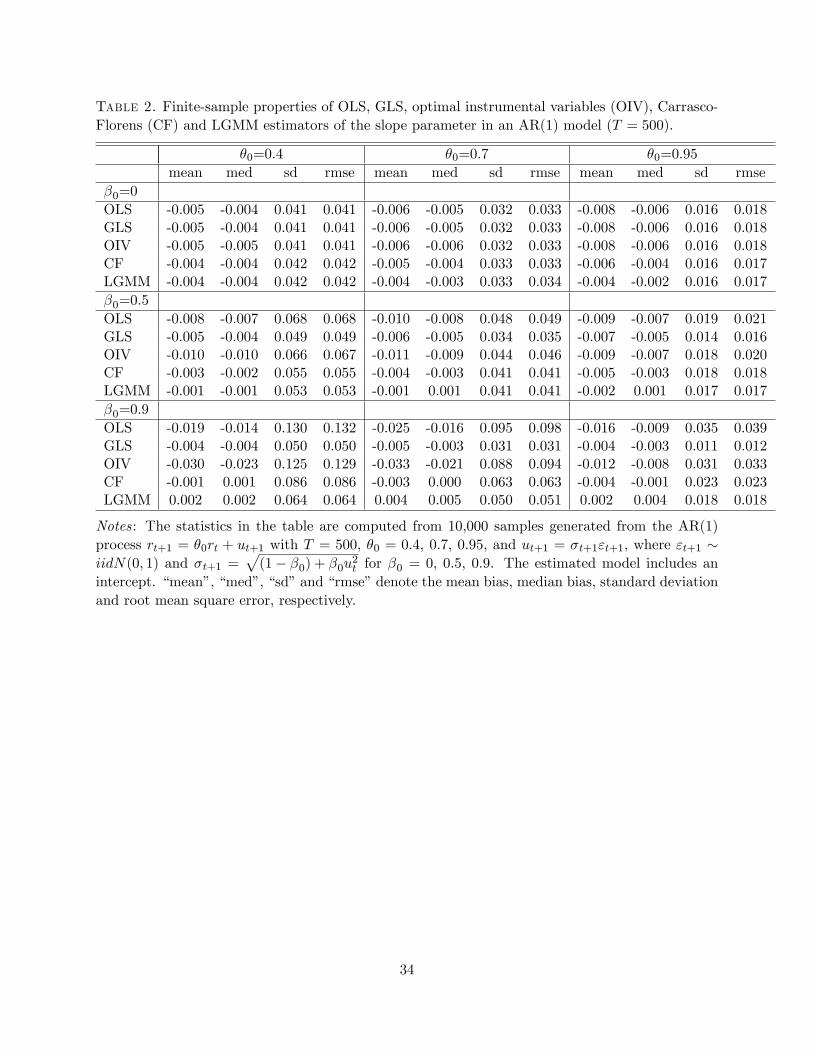
Table 2. Finite-sample properties of OLS, GLS, optimal instrumental variables (OIV), Carrasco-Florens (CF) and LGMM estimators of the slope parameter in an AR(1) model (T = 500).

�0=0:4 �0=0:7 �0=0:95mean med sd rmse mean med sd rmse mean med sd rmse

�0=0OLS -0.005 -0.004 0.041 0.041 -0.006 -0.005 0.032 0.033 -0.008 -0.006 0.016 0.018GLS -0.005 -0.004 0.041 0.041 -0.006 -0.005 0.032 0.033 -0.008 -0.006 0.016 0.018OIV -0.005 -0.005 0.041 0.041 -0.006 -0.006 0.032 0.033 -0.008 -0.006 0.016 0.018CF -0.004 -0.004 0.042 0.042 -0.005 -0.004 0.033 0.033 -0.006 -0.004 0.016 0.017LGMM -0.004 -0.004 0.042 0.042 -0.004 -0.003 0.033 0.034 -0.004 -0.002 0.016 0.017�0=0:5OLS -0.008 -0.007 0.068 0.068 -0.010 -0.008 0.048 0.049 -0.009 -0.007 0.019 0.021GLS -0.005 -0.004 0.049 0.049 -0.006 -0.005 0.034 0.035 -0.007 -0.005 0.014 0.016OIV -0.010 -0.010 0.066 0.067 -0.011 -0.009 0.044 0.046 -0.009 -0.007 0.018 0.020CF -0.003 -0.002 0.055 0.055 -0.004 -0.003 0.041 0.041 -0.005 -0.003 0.018 0.018LGMM -0.001 -0.001 0.053 0.053 -0.001 0.001 0.041 0.041 -0.002 0.001 0.017 0.017�0=0:9OLS -0.019 -0.014 0.130 0.132 -0.025 -0.016 0.095 0.098 -0.016 -0.009 0.035 0.039GLS -0.004 -0.004 0.050 0.050 -0.005 -0.003 0.031 0.031 -0.004 -0.003 0.011 0.012OIV -0.030 -0.023 0.125 0.129 -0.033 -0.021 0.088 0.094 -0.012 -0.008 0.031 0.033CF -0.001 0.001 0.086 0.086 -0.003 0.000 0.063 0.063 -0.004 -0.001 0.023 0.023LGMM 0.002 0.002 0.064 0.064 0.004 0.005 0.050 0.051 0.002 0.004 0.018 0.018

Notes: The statistics in the table are computed from 10,000 samples generated from the AR(1)process rt+1 = �0rt + ut+1 with T = 500; �0 = 0:4, 0:7, 0:95; and ut+1 = �t+1"t+1; where "t+1 �iidN(0; 1) and �t+1 =

p(1� �0) + �0u2t for �0 = 0; 0:5; 0:9. The estimated model includes an

intercept. �mean�, �med�, �sd�and �rmse�denote the mean bias, median bias, standard deviationand root mean square error, respectively.

34

Table 3. Bias properties of OLS and LGMM estimators of the slope parameter in a zero-meanAR(1) model with iid errors.

mean bias sd rmse E[A] E[B]

T = 50

OLS -0.0309 0.0646 0.0716 0.0002 0.0303LGMM -0.0128 0.0621 0.0634 0.0108 0.0310T = 100

OLS -0.0167 0.0395 0.0429 0.0000 0.0164LGMM -0.0040 0.0383 0.0385 0.0082 0.0168T = 200

OLS -0.0093 0.0260 0.0276 -0.0002 0.0090LGMM -0.0010 0.0258 0.0259 0.0055 0.0090T = 400

OLS -0.0048 0.0172 0.0178 0.0000 0.0048LGMM 0.0000 0.0173 0.0173 0.0034 0.0047T = 800

OLS -0.0026 0.0118 0.0121 -0.0001 0.0024LGMM 0.0001 0.0119 0.0119 0.0018 0.0024T = 1600

OLS -0.0011 0.0080 0.0081 0.0000 0.0012LGMM 0.0002 0.0081 0.0081 0.0011 0.0012T = 3200

OLS -0.0006 0.0055 0.0055 0.0000 0.0006LGMM 0.0001 0.0055 0.0055 0.0005 0.0006

Notes: The statistics in the table are computed from 5,000 samples generated from the AR(1)process rt+1 = �0rt + ut+1 with �0 = 0:95 and ut+1 � iidN(0; 1). �sd� and �rmse� denote thestandard deviation and root mean square error, respectively. The last two columns of the table areMonte Carlo averages of the terms E[AOLS ] and E[BOLS ] for the OLS estimator and E[ALGMM ]

and E[BLGMM ] for the LGMM estimator which are de�ned in Section 4.1.

35

Table 4. Finite-sample properties of GLS, Carrasco-Florens (CF) and LGMM estimators of theparameters of the CIR model and bond and option prices.

intercept � � � bond optiontrue 0.0184 0:2146 0:0857 0:0783 83.763 1.931GLSmedian 0.0488 0.5938 0.0825 0.0852 82.030 0.756mean 0.0587 0.6931 0.0866 0.0926 81.613 1.127sd 0.0455 0.4538 0.0279 0.0222 3.262 1.190rmse 0.0608 0.6595 0.0279 0.0264 3.907 1.436CFmedian 0.0497 0.6011 0.0826 0.0852 82.000 0.711mean 0.0586 0.6950 0.0864 0.0926 81.587 1.110sd 0.0407 0.4281 0.0273 0.0222 3.241 1.191rmse 0.0572 0.6435 0.0273 0.0264 3.904 1.446LGMMmedian 0.0328 0.4030 0.0833 0.0852 83.022 1.458mean 0.0403 0.4805 0.0873 0.0926 82.602 1.652sd 0.0324 0.3638 0.0297 0.0223 2.921 1.384rmse 0.0391 0.4506 0.0298 0.0265 3.143 1.412

Notes: The statistics in the table are computed from 5,000 samples generated from the CIR modelwith 4 = 1=52 and T = 600. �sd�and �rmse�denote the standard deviation and root mean squareerror, respectively. The prices of a three-year zero-coupon discount bond and a one-year Europeancall option on a three-year bond with face value of $100 and a strike price of $87 are computedanalytically as in Cox, Ingersoll and Ross (1985) with an initial interest rate of 5%. The �rst row�true�reports the true values of the parameters, bond and option prices.

36

T = 100 T = 200

Figure 1. Mean bias of OLS and LGMM estimators in a zero-mean AR(1) model with AR para-meter �0 = �0:95;�0:85; :::; 0:85; 0:95; and T = 100 (left graph) and T = 200 (right graph). TheLGMM estimators are computed with di¤erent bandwidths: (approximate) iid bandwidth T�1=5;0:6T�1=5 and 1:2T�1=5 with a standardized conditioning variable. The mean bias is computed from100,000 Monte Carlo replications.

37