Embed Size (px)
Citation preview

Local-Global Compatibility and theAction of Monodromy on nearby Cycles
The Harvard community has made thisarticle openly available. Please share howthis access benefits you. Your story matters
Citation Caraiani, Ana. 2012. Local-Global Compatibility and the Actionof Monodromy on nearby Cycles. Doctoral dissertation, HarvardUniversity.
Citable link http://nrs.harvard.edu/urn-3:HUL.InstRepos:10086046
Terms of Use This article was downloaded from Harvard University’s DASHrepository, and is made available under the terms and conditionsapplicable to Other Posted Material, as set forth at http://nrs.harvard.edu/urn-3:HUL.InstRepos:dash.current.terms-of-use#LAA
c©2012 – Ana CaraianiAll rights reserved.
Thesis advisor: Richard L. Taylor Author: Ana Caraiani
Local-global compatibility and the action ofmonodromy on nearby cycles
Abstract
In this thesis, we study the compatibility between local and global Langlands
correspondences for GLn. This generalizes the compatibility between local and
global class field theory and is related to deep conjectures in algebraic geometry
and harmonic analysis, such as the Ramanujan-Petersson conjecture and the
weight monodromy conjecture. Let L be a CM field. We consider the case when
Π is a cuspidal automorphic representation of GLn(A∞L ), which is conjugate
self-dual and regular algebraic. Under these assumptions, there is an l-adic
Galois representation Rl(Π) associated to Π, which is known to be compatible
with the local Langlands correspondence in most cases (for example, when n is
odd) and up to semisimplification in general. In this thesis, we complete the
proof of the compatibility when l "= p by identifying the monodromy operator
N on both the local and the global sides. On the local side, the identification
amounts to proving the Ramanujan-Petersson conjecture for Π as above. On
the global side it amounts to proving the weight-monodromy conjecture for part
of the cohomology of a certain Shimura variety.
iii
Contents
Abstract . . . . . . . . . . . . . . . . . . . . . . . . . . . . . . . . . . . iii
Table of Contents . . . . . . . . . . . . . . . . . . . . . . . . . . . . . . iv
Dedication . . . . . . . . . . . . . . . . . . . . . . . . . . . . . . . . . . vi
Acknowledgments . . . . . . . . . . . . . . . . . . . . . . . . . . . . . . vii
1 Introduction 1
1.1 Langlands correspondences and local-global compatibility . . . . 1
1.2 History of the problem . . . . . . . . . . . . . . . . . . . . . . . . 4
1.3 The results and methods of this thesis . . . . . . . . . . . . . . . 9
1.4 Organization of the thesis . . . . . . . . . . . . . . . . . . . . . . 13
2 An integral model 15
2.1 Shimura varieties . . . . . . . . . . . . . . . . . . . . . . . . . . . 15
2.2 An integral model for Iwahori level structure . . . . . . . . . . . 22
3 Sheaves of nearby cycles 39
3.1 Log structures . . . . . . . . . . . . . . . . . . . . . . . . . . . . . 40
3.2 Nearby cycles and log schemes . . . . . . . . . . . . . . . . . . . 42
4 The monodromy filtration 54
4.1 Overview of the strictly semistable case . . . . . . . . . . . . . . 54
iv

4.2 The product of strictly semistable schemes . . . . . . . . . . . . . 60
4.3 More general schemes . . . . . . . . . . . . . . . . . . . . . . . . 82
5 The cohomology of closed strata 95
5.1 Igusa varieties . . . . . . . . . . . . . . . . . . . . . . . . . . . . . 95
5.2 Counting points on Igusa varieties . . . . . . . . . . . . . . . . . 101
5.3 Vanishing of cohomology . . . . . . . . . . . . . . . . . . . . . . . 106
6 The cohomology of Igusa varieties 119
7 Proof of the main theorem 142
v
To Steven
Acknowledgments
First of all, I would like to thank my advisor, Richard Taylor, for suggesting
the topic of this dissertation and for his guidance, patience and generosity. This
thesis owes a tremendous debt to his insights and expertise. I owe to him my
mathematical development over the past five years and I am grateful for all that
he has taught me.
I am also greatly indebted to many mathematicians for their willingness
to share their insights and their knowledge with me, especially to Luc Illusie,
Sophie Morel, Arthur Ogus, Sug Woo Shin and Teruyoshi Yoshida. I am grateful
to Sophie Morel and Mark Kisin for reading this thesis and for their comments
and also to the anonymous referees, who provided much useful feedback.
I also benefitted a great deal from interacting with my fellow graduate stu-
dents at Harvard. I am grateful to them for useful conversations relevant to
this thesis as well as for creating a stimulating number theoretic environment
through numerous seminars and study groups. In particular, I am thankful to
Thomas Barnet-Lamb, Carl Erickson, David Geraghty, Wushi Goldring, Kather-
ine Korner, Bao Le Hung, Jay Pottharst, Sam Raskin, David Roe, Aaron Sil-
berstein, David Smyth and Jack Thorne. I am also grateful to the staff of the
Harvard Math Department, especially to Susan Gilbert, who made sure the
administrative part of my graduate studies went smoothly.
vii

CONTENTS viii
I am grateful to my closest friends for keeping me sane during graduate
school. I thank Nikola Kamburov and Silviu Pufu for ski trips, movie nights
and weekly brunch. I thank Tanya Khodorovskiy for teaching me many life
skills, among which how to make borscht. I thank Alice Zhou for thought-
provoking conversations over cookies and tea. I am also indebted to my fellow
fifth-years at Harvard, who created an exceptionally friendly and supportive
environment.
Finally, I would like to thank my family for all their love and support, es-
pecially my parents, Zoe and Cornel Caraiani, for always encouraging me to
pursue my passions; and my husband, Steven Sivek, for making me laugh every
day in the past seven years.

Chapter 1
Introduction
1.1 Langlands correspondences and local-global
compatibility
This thesis strengthens the compatibility of local and global Langlands corre-
spondences for GLn. The Langlands program provides a framework for gener-
alizing class field theory, one of the major achievements of 20th century number
theory, to the non-abelian setting. It is an intricate network of conjectures,
meant to unify different areas of mathematics, such as representation theory,
number theory and algebraic geometry. In the case of GLn, the Langlands pro-
gram predicts a global correspondence between automorphic representations of
GLn and n-dimensional Galois representations, which we state below.
Conjecture 1.1.1. (Langlands, Fontaine-Mazur) Let L be a number field and
l a rational prime. There is a bijection between the following sets consisting of
1

CHAPTER 1. INTRODUCTION 2
isomorphism classes:
{cuspidal automorphic
reps of GLn(AL)
algebraic
}↔
irred, cont. l-adic repsGal(L/L)→GLn(Ql)
unram. except at finitely many placesde Rham at l
.
The “cuspidal” condition on the automorphic side is expected to correspond
to the “irreducible” condition on the Galois side. The “algebraic” condition is
a condition on the infinitesimal character of the automorphic representation at
∞. This character can be thought of as a multiset of complex numbers via
the Harish-Chandra isomorphism and the requirement is that these complex
numbers be in fact integers. Its counterpart on the Galois side is the technical
requirement that the Galois representation be “de Rham at l”, which comes from
p-adic Hodge theory. This conjecture is known in many special cases, but it is
quite open in general. For n = 1, the conjecture is a consequence of global class
field theory.
At the same time, there is a local version of the Langlands correspondence,
which in the case of GLn was constructed by Harris and Taylor in 2001 [HT].
This correspondence generalizes local class field theory. If we let p be a rational
prime and K/Qp be a finite extension, then local class field theory gives a
canonical isomorphism
ArtK : K× → W abK ,
which takes uniformizers to geometric Frobenius elements.
We now let Irr(GLn(K)) denote the set of isomorphism classes of irreducible,
smooth representations of GLn(K) over C. Local Langlands is a correspondence
between Irr(GLn(K)) and certain objects very closely related to local Galois rep-
resentations, called Weil-Deligne representations. A Weil-Deligne representation
of the Weil group WK of K over C is a triple (V, r, N), where
• V is a finite-dimensional C-vector space

CHAPTER 1. INTRODUCTION 3
• r is a representation of WK on V with open kernel
• and N is a nilpotent endomorphism of V , which satisfies a certain com-
patibility with r, namely that for any σ ∈ WK
r(σ)Nr(σ)−1 = |Art−1K (σ)|KN.
Weil-Deligne representations of WK are roughly equivalent to continuous rep-
resentations of Gal(K/K). A Weil-Deligne representation is called Frobenius
semisimple if r is semisimple. Let WDRepn denote the set of isomorphism
classes of n-dimensional Frobenius semisimple Weil-Deligne representations of
WK over C.
Theorem 1.1.2. (Harris-Taylor, Henniart) For any finite extension K/Qp,
there exists a collection of bijections
recK : Irr(GLn(K)) → WDRepn(WK)
for every n ≥ 1 satisfying the following properties:
• for n = 1 the bijection is via composition with Art−1K .
• the bijection is compatible with twists by characters, with central characters
and with duals.
• for [π1] ∈ Irr(GLn1(K)) and [π2] ∈ Irr(GLn2(K)) then the L-factors and
ε-factors of π1 × π2 and rec(π1)⊗ rec(π2) are compatible.
The local and global correspondences are expected to be compatible, in the
same way that local and global class field theory are compatible. For exam-
ple, in the case of classsical modular forms, the compatibility ensures that the
eigenvalues of Frobenius on the Galois side match up with the Hecke eigenvalues

CHAPTER 1. INTRODUCTION 4
coming from the automorphic side. In general, the compatibility characterizes
the global correspondence uniquely and its precise statement is as follows.
Conjecture 1.1.3. (Local-global compatibility) Keep the notations as in Con-
jecture 1.1.1 and Theorem 1.1.2. Fix an isomorphism ιl : Ql * C. Let Π be
a cuspidal automorphic representation of GLn(AL) which is algebraic and let
Rl(Π) be the l-adic Galois representation associated to it.
Then for each place y of L above a rational prime p we have an isomorphism
of Weil-Deligne representations
WD(Rl(Π)|Gal(Ly/Ly))F−ss * ι−1
l recLy (Π∨y ⊗ |det|1−n
2 ).
1.2 History of the problem
The question of proving local-global compatibility has historically been in-
terwtined with the question of constructing Galois representations. This is the
traditional name for realizing the arrow
{cuspidal automorphic
reps Π of GLn(AL)
algebraic
}→
irred, cont. l-adic repsRl(Π):Gal(L/L)→GLn(Ql)
unram. except at finitely many placesde Rham at l
.
A general strategy is to find the Galois representation in the l-adic cohomology
of certain algebraic varieties, called Shimura varieties. Other than global class
field theory, the first major result in this direction goes back to Eichler-Shimura,
Deligne and Deligne-Serre who constructed Galois representations associated to
classical modular forms using modular curves.
For general n, a major breakthrough in the construction of Galois represen-
tations was obtained by Clozel [Cl1], who essentially constructed Rl(Π) under
the following conditions:

CHAPTER 1. INTRODUCTION 5
• L is a CM field,
• Π satisfies Π∨ * Π ◦ c, where c is complex conjugation,
• Π∞ is regular algebraic,
• Π is square-integrable at a finite place.
Roughly, the first two conditions ensure that Π comes an automorphic repre-
sentation of a unitary group via quadratic base change. The third condition
ensures that this automorphic reprsentation for a unitary group can be “seen”
in the cohomology of a unitary PEL-type Shimura variety. The fourth condition
ensures that one can work with a unitary group with trivial endoscopy, which
simplifies the trace formula used to compute the cohomology of the Shimura
variety.
Under the same conditions on Π, Harris and Taylor [HT] proved local-global
compatibility at all places of residual characteristic p "= l and up to semisimplifi-
cation. This means that they obtained an isomorphism of WK-representations,
but did not pin down the monodromy operator N coming from the global rep-
resentation Rl(Π). We comment briefly on the key geometric input of the ar-
gument. Harris and Taylor use a very special kind of Shimura variety, which,
in addition to having trivial endoscopy, is associated to a unitary group with
signature (1, n−1)×(0, n)× · · ·×(0, n) at infinity. It is a PEL-type Shimura va-
riety, which means that it is a moduli space for abelian varieties, equipped with
polarizations, endomorphisms and level structure. These abelian varieties have
to satisfy an important compatibility, called the Kottwitz determinant condition
[Ko1]. If one wants to compute Galois representations arising from cohomology
of the Shimura variety, locally at a place y of L, one can use an integral model
defined over the ring of integers OLy of Ly. This integral model is proper, but in
general not smooth. The moduli interpretation extends to the integral model,

CHAPTER 1. INTRODUCTION 6
however, and the Kottwitz determinant condition determines the structure of
the p-divisible group of each abelian variety (p here is the residue character-
istic of y). For signature (1, n − 1) × (0, n) × . . . (0, n), the p-divisible group
is essentially a one-dimensional Barsotti-Tate OLy - module. This leads to the
discovery that, in some sense, the singularities of the integral model are the
same as the singularities of the Lubin-Tate tower, whose cohomology realizes
the local Langlands correspondence.
Taylor and Yoshida [TY] extended the compatibility under the four con-
ditions above to Frobenius semisimplification. The idea for proving Conjec-
ture 1.3.1 in this case is to show that both WD(Rl(Π)|Gal(Ly/Ly)F−ss and
ι−1l Ln,Ly (Πy) have a remarkably elegant form, called “pure” in the terminol-
ogy of [TY]. A nice feature of purity is that it completely identifies the mon-
odromy operator. Moreover, purity reflects certain deep intuitions coming from
algebraic geometry and harmonic analysis.
To explain where the notion of purity originates, let K be a p-adic field for
p "= l.
Definition 1.2.1. A Weil-Deligne representation (V, r, N) of WK is called
“strictly pure of weight k” if the monodromy operator N = 0 and if every
eigenvalue of Frobenius is a Weil qk-number, where q is the cardinality of the
residue field of K.
From the Weil conjectures [De1, De2] it follows that the etale cohomology
of a proper, smooth variety over a finite field always gives rise to a strictly
pure Weil-Deligne representation. However, the etale cohomology of a proper,
smooth variety over K doesn’t have to be strictly pure, so a more general notion
is needed in this case.
Definition 1.2.2. A Weil-Deligne representation (V, r, N) is called “pure of
weight k” if V has an increasing filtration FilWi , with i ∈ k+Z whose ith graded
CHAPTER 1. INTRODUCTION 7
piece is strictly pure of weight i and such that N i induces an isomorphism
grWk+iV * grW
k−iV .
The weight-monodromy conjecture ([De2, I2, RZ]) states that the etale
cohomology of a proper, smooth variety over K always gives rise to a pure
Weil-Deligne representation. Therefore, identifying the monodromy operator in
WD(Rl(Π)|Gal(Ly/Ly)F−ss amounts to proving the weight-monodromy conjec-
ture for part of the cohomology of a Shimura variety with signature (1, n− 1)×
(0, n)× · · ·× (0, n).
On the other hand, the purity of ι−1l Ln,Ly (Πy) follows from the Ramanujan-
Petersson conjecture for Π as above. This conjecture predicts the fact that
the local components at finite places of cuspidal automorphic representations of
GLn(AL) (with unitary central characters) are tempered [Sar]. It is a general-
ization of the corresponding statement for Ramanujan’s ∆-function [Ra], which
followed from Deligne’s proof of the Weil conjectures [De1]. This conjecture, in
the case where Π is square-integrable at a finite place, had already been proved
by Harris and Taylor [HT] as a consequence of the Weil conjectures, since they
constructed Rl(Π) in the cohomology of a proper, smooth variety over L.
The key insight of [TY] is that it is possible to prove the weight-monodromy
conjecture for the Shimura variety with Iwahori level structure at y, in which
case the cohomology of the generic fiber can be computed via the Rapoport-Zink
weight spectral sequence. The inputs of the first page of the spectral sequence
are the cohomologies of closed Newton polygon strata in the special fiber of the
Shimura variety. These are proper, smooth schemes, whose cohomology realizes
parts of the representation ι−1l Ln,Ly (Πy)ss. Using the machinery of [HT], Taylor
and Yoshida compute the cohomology of each closed Newton polygon stratum
explicitly and prove that the Π∞-part of each cohomology is concentrated in the
middle dimension cohomology. Therefore, after restricting to the Π∞-part, the

CHAPTER 1. INTRODUCTION 8
first page of the Rapoport-Zink weight spectral sequence is concentrated on a di-
agonal and so the spectral sequence degenerates at the first page. This provides
exactly the filtration needed to prove the purity of WD(Rl(Π)|Gal(Ly/Ly)F−ss.
Harris-Taylor and Taylor-Yoshida therefore proved Conjecture 1.3.1 under
the assumption that Π is square-integrable at a finite place. Shin [Sh3] later
removed the condition that Π be square-integrable at a finite place, by working
with a unitary group with the same signature (1, n−1)×(0, n)× · · ·×(0, n), but
allowing endoscopy. He constructed Rl(Π) when n is odd and established full
local-global compatibility for l "= p. The difficulty when n is even comes from the
fact that there is a cohomological obstruction to the existence of a unitary group
with the desired signature at infinity and which is quasi-split. Shin found Rl(Π)
in the endoscopic part of the cohomology of a Shimura variety for n+1, but this
is only “visible” when Π∞ satisfies an additional regularity condition. Under
this condition, Shin again proved local-global compatibility in full for l "= p.
Chenevier and Harris [CH] then constructed the Galois representation in the
missing cases through a p-adic deformation argument. However, their argument
could only prove local-global compatibility for l "= p up to semisimplification.
In order to complete the proof of Conjecture 1.3.1 for L a CM field and Π
a conjugate self-dual, regular algebraic, cuspidal automorphic representation of
GLn(AL), one needs to treat the missing case of the compatibility: namely to
identify the monodromy operator in the case when n is even without any extra
assumptions on Π∞. We remark that in this thesis we are concerned with local-
global compatibility at primes p "= l. Simultaneously with writing this thesis,
there has been a huge amount of progress in proving local-global compatibility
when p = l: the papers of Barnet-Lamb, Gee Geraghty and Taylor [BLGGT1,
BLGGT2] prove the compatibility for l = p under the same assumptions as
[Sh3, CH]. We have, since then, also found a way to identify the monodromy
CHAPTER 1. INTRODUCTION 9
operator when l = p and n is even [Car], using different methods than those of
this thesis.
1.3 The results and methods of this thesis
In this thesis we complete the proof of the following theorem.
Theorem 1.3.1. Let n ∈ Z≥2 be an integer and L be any CM field with complex
conjugation c. Let l be a prime of Q and ιl be an isomorphism ιl : Ql → C. Let
Π be a cuspidal automorphic representation of GLn(AL) satisfying
• Π∨ * Π ◦ c
• Π is regular algebraic (this is the same as asking Π to be cohomological for
some irreducible algebraic representation Ξ of GLn(L⊗Q C)).
Let
Rl(Π) : Gal(L/L) → GLn(Ql)
be the Galois representation associated to Π by [Sh3, CH]. Let p "= l and let y be
a place of L above p. Then we have the following isomorphism of Weil-Deligne
respresentations
WD(Rl(Π)|Gal(Ly/Ly))F−ss * ι−1
l Ln,Ly (Πy).
Here Ln,Ly (Πy) = rec(Π∨y ) ⊗ |det| 1−n2 is the image of Πy under the local
Langlands correspondence, where the geometric normalization is used.
In the process of proving Theorem 1.3.1, we also prove the Ramanujan-
Petersson conjecture for Π as above.
Theorem 1.3.2. Let n ∈ Z≥2 be an integer and L be any CM field. Let Π be
a cuspidal automorphic representation of GLn(AL) satisfying

CHAPTER 1. INTRODUCTION 10
• Π∨ * Π ◦ c
• Π∞ is cohomological for some irreducible algebraic representation Ξ of
GLn(L⊗Q C).
Then Π is tempered at any finite place of L.
As mentioned in Section 1.2, the above theorems are already known when
n is odd or when n is even and Π is slightly regular, by work of Shin [Sh3].
They are also known if Π is square integrable at a finite place, by the work
of Harris-Taylor [HT] and Taylor-Yoshida [TY]. If n is even then Chenevier
and Harris construct in [CH] a global Gal(L/L)-representation Rl(Π) which is
compatible with the local Langlands correspondence up to semisimplification.
Theorem 1.3.2 was proven by Clozel [Cl2] at the places where Π is unramified.
We extend the local-global compatibility up to Frobenius semisimplification, by
proving that both Weil-Deligne representations are pure.
The fact that ι−1l Ln,Ly (Πy) is pure of some weight follows once we know The-
orem 1.3.2 for all σΠ, where σ ∈ Aut(C). For the representation WD(Rl(Π)|Gal(Ly/Ly)),
our strategy is as follows: we find the Galois representation Rl(Π)⊗2 in the co-
homology of a system of Shimura varieties XU associated to a unitary group
which looks like
U(1, n− 1)× U(1, n− 1)× U(0, n)d−2
at infinity. Following the same structure of argument as Taylor-Yoshida in [TY],
we prove that the Weil-Deligne representation associated to
Rl(Π)⊗2|Gal(Ly/L)
is pure by explicitly computing the action of the monodromy operator N on

CHAPTER 1. INTRODUCTION 11
the cohomology of the system of Shimura varieties. We use Theorem 1.3.2 at a
crucial point in the computation. We conclude that WD(Rl(Π)|Gal(Ly/Ly))F−ss
must also be pure of some weight.
To summarize, there are two main parts to the argument: a geometric input
and a representation-theoretic input. The geometric input computes the action
of the monodromy operator on the complex of nearby cycles on a certain kind
of proper, but not smooth, scheme. This does not depend so much on the fact
that the scheme we work with is a Shimura variety. The representation-theoretic
input proves the Ramanujan-Petersson conjecture via a stable trace formula for
computing the cohomology of Shimura varieties or other closely related varieties.
We start by explaining the geometric input, i.e. we briefly outline our com-
putation of the action of N on the Weil-Deligne representation associated to
Rl(Π)⊗2|Gal(Ly/Ly). First, we base change Π to a CM field F ′ such that there is
a place p of F ′ above the place y of L where BCF ′/L(Π)p has an Iwahori fixed
vector. It suffices to study the Weil-Deligne representation corresponding to
Π0 = BCF ′/L(Π) and prove that it is pure. We then take a quadratic extension
F of F ′ which is also a CM field and in which the place p splits p = p1p2. We
let σ ∈ Gal(F/F ′) be the automorphism which sends p1 to p2. We choose F
and F ′ such that they contain an imaginary quadratic field E in which p splits.
We take a Q-group G which satisfies the following:
• G is quasi-split at all finite places.
• G(R) has signature (1, n − 1) at two embeddings which differ by σ and
(0, n) everywhere else.
• G(AE) * GL1(AE)×GLn(AF ).
We let Π1 = BCF/F ′(Π0). Then the Galois representation Rl(Π0) can be seen
in the Π1,∞-part of the (base change of the) cohomology of a system of Shimura

CHAPTER 1. INTRODUCTION 12
varieties associated to G. We let XU be the inverse system of Shimura varieties
associated to the group G. We let the level U vary outside p1p2 and be equal
to the Iwahori subgroup at p1 and p2. We construct an integral model of XU
which parametrizes abelian varieties with Iwahori level structure at p1 and p2.
By abuse of notation, we will denote this integral model by XU as well. The
special fiber YU of XU has a stratification by YU,S,T where the S, T ⊆ {1, . . . n}
are related to the Newton polygons of the p-divisible groups above p1 and p2.
We compute the completed strict local rings at closed geometric points of XU
and use this computation to show that XU is locally etale over a product of
strictly semistable schemes, which on the special fiber are closely related to the
strata YU,S,T . If we let AU be the universal abelian variety over XU , then AU
has the same stratification and the same geometry as XU .
Let ξ be an irreducible algebraic representation of G over Ql, which deter-
mines non-negative integers tξ, mξ and an endomorphism aξ ∈ End(Amξ
U /XU )⊗Z
Q. We are interested in understanding the Π1,∞-part of
Hj(XU ,Lξ) = aξHj+mξ(Amξ
U , Ql(tξ)).
Thus, we study the cohomology of the generic fiber Hj(Amξ
U , Ql) and we do
so via the cohomology of the complex of nearby cycles RψQl over the special
fiber of Amξ
U . The key ingredients in studying the complex of nearby cycles
together with the action of monodromy are logarithmic schemes, the weight
spectral sequence as constructed by Saito [Sa2] (which on the level of complexes
of sheaves describes the action of monodromy on the complex of nearby cycles
for strictly semistable schemes), and the formula
(RψQl)X1×X2 * (RψQl)X1 ⊗L (RψQl)X2 ,

CHAPTER 1. INTRODUCTION 13
when X1 and X2 are semistable schemes. Using these ingredients, we deduce
the existence a spectral sequence relating terms of the form Hj(Amξ
U,S,T , Ql)
(up to twisting and shifting) to the object we’re interested in, Hj(Amξ
U , Ql).
This spectral sequence is, in some sense, a generalization of the Rapoport-Zink
spectral sequence [RZ] for a strictly semistable scheme to the case of a scheme
which looks locally like a product of strictly semistable schemes.
At this stage, the representation-theoretic input comes into play. The coho-
mology of each stratum Hj(Amξ
U,S,T , Ql) is closely related to the cohomology of
Igusa varieties. The next step is to compute the Π1,∞-part of the cohomology of
certain Igusa varieties, for which we adapt the strategy of Theorem 6.1 of [Sh3]
and the stable trace formula deduced in [Sh2]. Using the result on Igusa vari-
eties, we prove Theorem 1.3.2 and then we also make use of the classification of
tempered representations. We prove that the Π1,∞-part of each Hj(Amξ
U,S,T , Ql)
vanishes outside the middle dimension and thus that our spectral sequence de-
generates at E1. The E1 page of the spectral sequence provides us with the
exact filtration of the Π1,∞-part of
lim−→Up
H2n−2(XU ,Lξ)
which exhibits its purity.
1.4 Organization of the thesis
We now describe the organization of this thesis. In Chapter 2 we define the
PEL datum, unitary group and Shimura varieties we shall work with, we define
integral models for these Shimura varieties as well as stratifications of their
special fibers. We study the geometry of the integral model with Iwahori level
structure, both globally, in terms of the stratification, and locally, in which case

CHAPTER 1. INTRODUCTION 14
it essentially looks like a product of strictly semistable schemes.
In Chapter 3 we define a log structure over the Shimura variety with Iwahori
level structure and show that this log structure gives rise to a log smooth scheme.
We review and use Nakayama’s results on nearby cycles for log smooth schemes
[Na], computing the sheaves of nearby cycles on our Shimura variety explicitly.
We also review Illusie’s computation of the complex of nearby cycles in the case
of a product of strictly semistable schemes [I2].
In Chapter 4 we review Saito’s construction of the weight spectral sequence
for a strictly semistable schemes [Sa2], but motivate it using log schemes and
log structures. We then use the computations in Chapter 3 to identify the
monodromy filtration on the complex of nearby cycles, first in the case of a
product of strictly semistable schemes, then in the case matching our Iwahori-
level Shimura variety. This makes use of the framework of perverse sheaves. We
obtain our spectral sequence relating the cohomologies of the closed Newton
polygon strata to the cohomology of the Iwahori-level Shimura variety.
In Chapter 5 we relate the closed Newton polygon strata to Igusa varieties,
we prove Theorem 1.3.2 (the Ramanujan-Petersson conjecture) and we show
that the Π∞-part of the cohomology of the closed Newton polygon strata van-
ishes outside the middle dimension. The results of Chapter 5 depend on a
cohomological computation for Igusa varieties, which we defer until the next
chapter.
In Chapter 6 we use Shin’s stable trace formula for Igusa varieties [Sh2] to
compute the cohomology of the Igusa varieties we’re working with. This section
follows [Sh3] very closely and makes use of the trace formula, endoscopy (which
we show plays a trivial part in our case) and local base change.
In Chapter 7 we put the results of the previous chapters together and prove
the main theorem, Theorem 1.3.1.

Chapter 2
An integral model
2.1 Shimura varieties
Let E be an imaginary quadratic field in which p splits, let c be the non-trivial
element in Gal(E/Q) and choose a prime u of E above p. From now on, we
assume that n is an even positive integer.
Let F1 be a totally real field of finite degree over Q and w a prime of F1 above
p. Let F2 be a quadratic totally real extension of F1 in which w splits w = w1w2.
Let d = [F2 : Q] and we assume that d ≥ 3. Let F = F2.E. Let pi be the prime
of F above wi and u for i = 1, 2. We denote by pi for 2 < i ≤ r the rest of the
primes which lie above the prime u of E. We choose embeddings τi : F ↪→ C
with i = 1, 2 such that τ2 = τ1 ◦ σ, where σ is the element of Gal(F/Q) which
takes p1 to p2. In particular, this means that τE := τ1|E = τ2|E is well-defined.
By abuse of notation we will also denote by σ the Galois automorphism of F2
taking w1 to w2.
We will work with a Shimura variety corresponding to the PEL datum
(F, ∗, V, 〈·, ·〉, h), where F is the CM field defined above and ∗ = c is the in-
15

CHAPTER 2. AN INTEGRAL MODEL 16
volution given by complex conjugation. We take V to be the F -vector space Fn
for some integer n. The pairing
〈·, ·〉 : V × V → Q
is a non-degenerate Hermitian pairing such that 〈fv1, v2〉 = 〈v1, f∗v2〉 for all
f ∈ F and v1, v2 ∈ V . The last element we need is an R-algebra homomorphism
h : C → EndF (V )⊗Q R such that the bilinear pairing
(v1, v2) → 〈v1, h(i)v2〉
is symmetric and positive definite.
We define an algebraic group G over Q by
G(R) = {(g, λ) ∈ EndF⊗QR(V ⊗Q R)×R× | 〈gv1, gv2〉 = λ〈v1, v2〉}
for any Q-algebra R. For σ ∈ HomE,τE (F, C) we let (pσ, qσ) be the signature
at σ of the pairing 〈·, ·〉 on V ⊗Q R. We claim that we can find a PEL datum
as above, such that (pτ , qτ ) = (1, n − 1) for τ = τ1 or τ2 and (pτ , qτ ) = (0, n)
otherwise and such that GQv is quasi-split at every finite place v.
Lemma 2.1.1. Let F be a CM field as above. For any embeddings τ1, τ2 : F ↪→
C there exists a PEL datum (F, ∗, V, 〈·, ·〉, h) as above such that the associated
group G is quasi-split at every finite place and has signature (1, n−1) at τ1 and
τ2 and (0, n) everywhere else.
Proof. This lemma is standard and follows from computations in Galois coho-
mology found in section 2 of [Cl1], but see also Lemma 1.7 of [HT]. The problem
is that of constructing a global unitary similitude group with prescribed local
conditions. It is enough to consider the case of a unitary group G0 over Q,
CHAPTER 2. AN INTEGRAL MODEL 17
by taking it to be the algebraic group defined by ker(G(R) → R×) sending
(g,λ) 2→ λ.
A group G defined as above has a quasi-split inner form over Q denoted Gn,
defined as in section 3 of [Sh3]. This inner form Gn is the group of similitudes
which preserve the non-degenerate Hermitian pairing 〈v1, v2〉 = v1ζΦtvc2 with
Φ ∈ GLn(Q) having entries
Φij = (−1)i+1δi,n+1−j
and ζ ∈ F ∗ an element of trace 0. Let G′ be the adjoint group of G0n. It suffices
to show that the tuple of prescribed local conditions, classified by elements in
⊕vH1(F2,v, G′), is in the image of the map
H1(F2, G′) → ⊕vH1(F2,v, G′),
where the sum is taken over all places v of F2. For n odd, Lemma 2.1 of [Cl1]
ensures that the above map is surjective, so there is no cohomological obstruction
for finding the global unitary group. In the case we are interested in, n is even
and the image of the above map is equal to the kernel of
⊕
v
H1(F2,v, G′) → Z/2Z.
We can use Lemma 2.2 of [Cl1] to compute all the local invariants (i.e. the
images of H1(F2,v, G′) → Z/2Z for all places v). At the finite places, the sum of
the invariants is 0 (mod 2) (this is guaranteed by the existence of the quasi-split
inner form Gn of G, which has the same local invariants at finite places). At
the infinite places τ1 and τ2 the invariants are n2 + 1 (mod 2) and at all other
infinite places they are n2 (mod 2). The global invariant is nd
2 + 2 (mod 2),

CHAPTER 2. AN INTEGRAL MODEL 18
where d is the degree of F2 over Q. Since d is even, the image in Z/2Z is equal
to 0 (mod 2), so the prescribed local unitary groups arise from a global unitary
group.
We will choose the R-homomorphism h :C → EndF (V )⊗Q R such that under
the natural R-algebra isomorphism EndF (V )R *∏
τ |E=τEMn(C) it equals
z 2→
zIpτ 0
0 zIqτ
τ
,
where τ runs over elements of HomE,τE (F, C).
Now that we’ve defined the PEL datum we can set up our moduli problem.
Note that the reflex field of the PEL datum is F ′ = F1 · E. Let S/F ′ be
a scheme and A/S an abelian scheme of dimension dn. Suppose we have an
embedding i : F ↪→ End(A) ⊗Z Q. LieA is a locally free OS-module of rank
dn with an action of F . We can decompose LieA = Lie+A ⊕ Lie−A where
Lie+A = LieA ⊗OS⊗E OS and the map E ↪→ F ′ → OS is the natural map
followed by the structure map. Lie−A is defined in the same way using the
complex conjugate of the natural map E ↪→ F ′. We ask that Lie+A be a free
OS-module of rank 2 and that Lie+A * OS ⊗F1 F2 as an OS-module with an
action of F2.
Definition 2.1.2. If the the conditions above are satisfied, we will call the pair
(A, i) compatible.
Remark. This is an adaptation to our situation of the notion of compatibility de-
fined in section III.1 of [HT], which fulfills the same purpose as the determinant
condition defined on page 390 of [Ko1].
For an open compact subgroup U ⊂ G(A∞) we consider the contravariant
CHAPTER 2. AN INTEGRAL MODEL 19
functor XU mapping
Connected, locally noetherian
F ′-schemes with geometric point
(S, s)
→ (Sets)
(S, s) 2→ {(A, λ, i, η)}/ ∼
where
• A is an abelian scheme over S;
• λ : A → A∨ is a polarization;
• i : F ↪→ End0(A) = EndA ⊗Z Q is such that (A, i) is compatible and
λ ◦ i(f) = i(f∗)∨ ◦ λ, for all f ∈ F ;
• η is a π1(S, s)-invariant U -orbit of isomorphisms of Hermitian F ⊗Q A∞-
modules
η : V ⊗Q A∞ → V As
which take the fixed pairing 〈·, ·〉 on V to on (A∞)×-multiple of the λ-Weil
pairing on V As. Here,
V As =(lim←
A[N ](k(s)))⊗Z Q
is the adelic Tate module.
We consider two quadruples as above equivalent if there is an isogeny between
the abelian varieties which is compatible with the additional structures. If s′
is a different geometric point of S then there is a canonical bijection between
XU (S, s) and XU (S, s′). We can forget about the geometric points and extend
the definition from connected to arbitrary locally noetherian F ′-schemes. When

CHAPTER 2. AN INTEGRAL MODEL 20
U is sufficiently small, this functor is representable by a smooth and quasi-
projective variety XU/F ′ of dimension 2n− 2 (this is explained on page 391 of
[Ko1]). The variety XU is a disjoint union of | ker1(G, Q)| copies of the canonical
model of the Shimura variety. As U varies, the inverse system of the XU has a
natural right action of G(A∞).
Let AU be the universal abelian variety over XU . The action of G(A∞) on
the inverse system of the XU extends to an action by quasi-isogenies on the
inverse system of the AU . The following construction goes through as in section
III.2 of [HT]. Let l be a rational prime (we impose no conditions on l yet, but we
will restrict to l different from p when we work with an integral model over the
ring of integers in a p-adic field) and let ξ an irreducible algebraic representation
of G over Qacl . This defines a lisse Qac
l -sheaf Lξ,l over each XU and the action
of G(A∞) extends to the inverse system of sheaves. The direct limit
Hi(X,Lξ,l) = lim→
Hi(XU ×F ′ F′,Lξ,l)
is a (semisimple) admissible representation of G(A∞) with a continuous action
of Gal(F ′/F ′). We can decompose it as
Hi(X,Lξ,l) =⊕
π
π ⊗Riξ,l(π)
where the sum runs over irreducible admissible representations π of G(A∞)
over Qacl . The Ri
ξ,l(π) are finite dimensional continuous representations of
Gal(F ′/F ′) over Qacl . We shall suppress the l from Lξ.l and Ri
ξ,l(π) where
it is understood from context. To the irreducible representation ξ of G we can
associate as in section III.2 of [HT] non-negative integers mξ and tξ and an
idempotent εξ ∈ Q[Smξ ] (where Smξ is the symmetric group on mξ letters). As
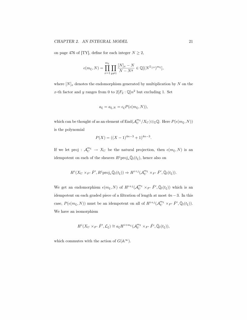
CHAPTER 2. AN INTEGRAL MODEL 21
on page 476 of [TY], define for each integer N ≥ 2,
ε(mξ, N) =mξ∏
x=1
∏
y +=1
[N ]x −N
N −Ny∈ Q[(NZ≥0)mξ ],
where [N ]x denotes the endomorphism generated by multiplication by N on the
x-th factor and y ranges from 0 to 2[F2 : Q]n2 but excluding 1. Set
aξ = aξ,N = εξP (ε(mξ, N)),
which can be thought of as an element of End(Amξ
U /XU )⊗ZQ. Here P (ε(mξ, N))
is the polynomial
P (X) = ((X − 1)4n−3 + 1)4n−3.
If we let proj : Amξ
U → XU be the natural projection, then ε(mξ, N) is an
idempotent on each of the sheaves Rjproj∗Ql(tξ), hence also on
Hi(XU ×F ′ F′, Rjproj∗Ql(tξ)) ⇒ Hi+j(Amξ
U ×F ′ F′, Ql(tξ)).
We get an endomorphism ε(mξ, N) of Hi+j(Amξ
U ×F ′ F ′, Ql(tξ)) which is an
idempotent on each graded piece of a filtration of length at most 4n− 3. In this
case, P (ε(mξ, N)) must be an idempotent on all of Hi+j(Amξ
U ×F ′ F ′, Ql(tξ)).
We have an isomorphism
Hi(XU ×F ′ F′,Lξ) ∼= aξH
i+mξ(Amξ
U ×F ′ F ′, Ql(tξ)),
which commutes with the action of G(A∞).
CHAPTER 2. AN INTEGRAL MODEL 22
2.2 An integral model for Iwahori level structure
Let K = Fp1 * Fp2 , where the isomorphism is via σ, denote by OK the ring of
integers of K and by π a uniformizer of OK .
Let S/OK be a scheme and A/S an abelian scheme of dimension dn. Suppose
we have an embedding i : OF ↪→ End(A) ⊗Z Z(p). LieA is a locally free OS-
module of rank dn with an action of F . We can decompose LieA = Lie+A ⊕
Lie−A where Lie+A = LieA⊗Zp⊗OE OE,u. There are two natural actions of OF
on Lie+A, via OF → OFpj
∼→ OK composed with the structure map for j = 1, 2.
These two actions differ by the automorphism σ ∈ Gal(F/Q). There is also a
third action via the embedding i of OF into the ring of endomorphisms of A.
We ask that Lie+A be locally free of rank 2, that the part of Lie+A where the
first action of OF on Lie+A coincides with i be locally free of rank 1 and that
the part where the second action coincides with i also be locally free of rank 1.
Definition 2.2.1. If the above conditions are satisfied, then we call (A, i) com-
patible. One can check that for S/K this notion of compatibility coincides with
the one in Definition 2.1.2.
If p is locally nilpotent on S then (A, i) is compatible if and only if
• A[p∞i ] is a compatible, one-dimensional Barsotti-Tate OK-module for i =
1, 2 and
• A[p∞i ] is ind-etale for i > 2.
By a compatible Barsotti-Tate OK-module we mean that the two actions on it
by OK , via endomorphisms or via the structure map coincide.
We will now define a few integral models for our Shimura varieties XU . We
can decompose G(A∞) as
G(A∞) = G(A∞,p)×Q×p ×r∏
i=1
GLn(Fpi).

CHAPTER 2. AN INTEGRAL MODEL 23
For each i, let Λi be an OFpi-lattice in Fn
piwhich is stable under GLn(OFpi
)
and self-dual with respect to 〈·, ·〉. For each -m = (m1, . . . ,mr) and compact
open Up ⊂ G(A∞,p) we define the compact open subgroup Up(-m) of G(A∞) as
Up(-m) = Up × Z×p ×r∏
i=1
ker(GLOFpi(Λi) → GLOFpi
(Λi/mmiFpi
Λi)).
The corresponding moduli problem of sufficiently small level Up(-m) over OK is
given by the functor
Connected, locally noetherian
OK-schemes with geometric point
(S, s)
→ (Sets)
(S, s) 2→ {(A, λ, i, ηp, {αi}ri=1)}/ ∼
where
• A is an abelian scheme over S;
• λ : A → A∨ is a prime-to-p polarization;
• i : OF ↪→ End(A) ⊗Z Z(p) such that (A, i) is compatible and λ ◦ i(f) =
i(f∗)∨ ◦ λ,∀f ∈ OF ;
• ηp is a π1(S, s)-invariant Up-orbit of isomorphisms of Hermitian F ⊗Q
A∞,p-modules
η : V ⊗Q A∞,p → V pAs
which take the fixed pairing 〈·, ·〉 on V to an (A∞,p)×-multiple of the λ-
Weil pairing on V As. Here V pAs is the adelic Tate module away from
p;
• for i = 1, 2, αi : p−mii Λi/Λi → A[pmi
i ] is a Drinfeld pmii -structure, i.e. the

CHAPTER 2. AN INTEGRAL MODEL 24
set of αi(x), x ∈ (p−mii Λi/Λi) forms a full set of sections of A[pmi
i ] in the
sense of section 1.8 of [KM];
• for i > 2, αi : (p−mii Λi/Λ) ∼→ A[pmi
i ] is an isomorphism of S-schemes with
OFpi-actions;
• Two tuples (A, λ, i, ηp, {αi}ri=1) and (A′, λ′, i′, (ηp)
′, {α′i}r
i=1 are equivalent
if there is a prime-to-p isogeny A → A′ taking λ, i, ηp, αi to γλ′, i′, (ηp)′, α′i
for some γ ∈ Z×(p).
This moduli problem is representable by a projective scheme overOK , which will
be denoted XUp,%m. The projectivity follows from Theorem 5.3.3.1 and Remark
5.3.3.2 of [Lan]. If m1 = m2 = 0 this scheme is smooth as in Lemma III.4.1.2 of
[HT], since we can check smoothness on the completed strict local rings at closed
geometric points and these are isomorphic to deformation rings for p-divisible
groups (with level structure only at pi for i > 2, when the p-divisible group is
etale). Moreover, if m1 = m2 = 0 the dimension of XUp,%m is 2n− 1.
When m1 = m2 = 0, we will denote XUp,%m by XU0 . If AU0 is the universal
abelian scheme over XU0 we write Gi = AU0 [p∞i ] for i = 1, 2 and G = G1 × G2.
Over a base where p is nilpotent, each of the Gi is a one-dimensional compatible
Barsotti-Tate OK-module.
Let F be the residue field of OK . Let XU0 = XU0 ×Spec OKSpec F be the
special fiber of XU0 . We define a stratification on XU0 in terms of 0 ≤ h1, h2 <
n− 1. The scheme X [h1,h2]U0
will be the reduced closed subscheme of XU0 whose
closed geometric points s are those for which the maximal etale quotient of Gi
has OK-height at most hi. Let X(h1,h2)U0
= X [h1,h2]U0
− (X [h1−1,h2]U0
∪ X [h1,h2−1]U0
).
Lemma 2.2.2. The scheme X(h1,h2)U0
is non-empty and smooth of pure dimen-
sion h1 + h2.
Proof. In order to see that this is true, note that the formal completion of XU0

CHAPTER 2. AN INTEGRAL MODEL 25
at any closed point is isomorphic to F[[T2, . . . , Tn, S2, . . . , Sn]] since it is the uni-
versal formal deformation ring of a product of two one-dimensional compatible
Barsotti-Tate groups of height n each. (In fact it is the product of the universal
deformation rings for each of the two Barsotti-Tate groups.) Thus, XU0 has
dimension 2n − 2 and as in Lemma II.1.1 of [HT] each closed stratum X [h1,h2]U0
has dimension at least h1 + h2. The lower bound on dimension also holds for
each open stratum X(h1,h2)U0
. In order to get the upper bound on the dimension
it suffices to show that the lowest stratum X(0,0)U0
is non-empty. Indeed, once
we have a closed point s in any stratum X(h1,h2)U0
, we can compute the formal
completion (X(h1,h2)U0
)∧s as in Lemma II.1.3 of [HT] and find that the dimen-
sion is exactly h1 + h2. We start with a closed point of the lowest stratum
X(0,0)U0
= X [0,0]U0
and prove that this stratum has dimension 0. The higher closed
strata X [h1,h2]U0
= ∪j1≤h1,j2≤h2X(j1,j2)U0
are non-empty and it follows by induction
on (h1, h2) that the open strata X(h1,h2)U0
are also non-empty.
It remains to see that X(0,0)U0
is non-empty. This can be done using Honda-
Tate theory as in the proof of Corollary V.4.5. of [HT], whose ingredients
for Shimura varieties associated to more general unitary groups are supplied
in sections 8 through 12 of [Sh1]. In our case, Honda-Tate theory exhibits a
bijection between p-adic types over F (see section 8 of [Sh1] for the general
definition) and pairs (A, i) where A/F is an abelian variety of dimension dn and
i : F ↪→ End(A) ⊗Z Q. The abelian variety A must also satisfy the following:
A[p∞i ] is ind-etale for i > 2 and A[p∞i ] is one-dimensional of etale height hi
for i = 1, 2. Note that the slopes of the p-divisible groups A[p∞i ] are fixed for
all i. All our p-adic types will be simple and given by pairs (M, η) where M
is a CM field extension of F and η ∈ Q[P] where P is the set of places of M
above p. The coefficients in η of places x of M above pi are related to the slope
of the corresponding p-divisible group at pi as in Corollary 8.5 of [Sh3]. More

CHAPTER 2. AN INTEGRAL MODEL 26
precisely, A[x∞] has pure slope ηx/ex/p. It follows that the coefficients of η at
places x and xc above p satisfy the compatibility
ηx + ηxc = ex/p
so to know η it is enough to specify ηx · x as x runs through places of M above
u.
In order to exhibit a pair (A, i) with the right slope of A[p∞i ] it suffices to
exhibit its corresponding p-adic type. For this, we can simply take M = F and
ηpi = epi/p
n[Fpi :Qp] · pi for i = 1, 2 and ηpi = 0 otherwise. The only facts remaining
to be checked are that the associated pair (A, i) has a polarization λ which
induces c on F and that the triple (A, i,λ) can be given additional structure
to make it into a point on X(0,0)U0
. First we endow (A, i) with a polarization
λ0 for which the Rosati involution induces c on F using Lemma 9.2 of [Ko1]
and we use Lemma 5.2.1, an analogue of Lemma V.4.1 of [HT], to construct an
F -module W0 together with a non-degenerate Hermitian pairing such that
W0 ⊗ A∞,p * V pA and W0 ⊗Q R * V ⊗Q R
as Hermitian F ⊗Q A∞,p-modules (F ⊗Q R-modules respectively). Then we use
the difference (in the Galois cohomology sense) between W0 and V as Hermitian
F -modules over Q to find a polarization λ such that V pA with its λ-Weil pairing
is equivalent to V ⊗ A∞,p with its standard pairing, as in Lemma V.4.3 of
[HT]. Note that the argument is not circular, since the proof of Lemma 5.2.1 is
independent of this section.
The next Lemma is an analogue of Lemma 3.1 of [TY].
Lemma 2.2.3. If 0 ≤ h1, h2 ≤ n − 1 then the Zariski closure of X(h1,h2)U0
contains X(0,0)U0
.

CHAPTER 2. AN INTEGRAL MODEL 27
Proof. The proof follows exactly like the proof of Lemma 3.1 of [TY]. Let x be
a closed geometric point of X(0,0)U0
. The main point is to note that the formal
completion of XU0×Spec F at x is isomorphic to the equicharacteristic universal
deformation ring of G1,x × G2,x, so it is isomorphic to
Spf F[[T2, . . . , Tn, S2, . . . , Sn]].
We can choose the Ti, the Si and formal parameters X on the universal defor-
mation of G1,x and Y on the universal deformation of G2,x such that
[π](X) ≡ πX +n∑
i=2
TiX#Fi−1
+ X#Fn
(mod X#Fn+1) and
[π](Y ) ≡ πY +n∑
i=2
SiX#Fi−1
+ S#Fn
(mod S#Fn+1).
We get a morphism
Spec F[[T2, . . . , Tn, S2, . . . , Sn]] → XU0
lying over x : Spec F → XU0 such that if k denotes the algebraic closure of the
field of fractions of
Spec F[[T2, . . . , Tn, S2, . . . Sn]]/(T2, . . . , Tn−h1 , S2, . . . , Sn−h2)
then the induced map Spec k → XU0 factors through X(h1,h2)U0
.
For i = 1, 2, let Iwn,pi be the subgroup of matrices in GLn(OK) which
reduce modulo pi to Bn(F) (here Bn(F) ⊂ GLn(F) is the Borel subgroup). We
will define an integral model for XU , where U ⊆ G(A∞) is equal to
Up × Up1,p2p (-m)× Iwn,p1 × Iwn,p2 × Z×p .
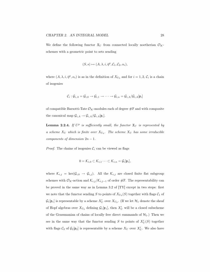
CHAPTER 2. AN INTEGRAL MODEL 28
We define the following functor XU from connected locally noetherian OK-
schemes with a geometric point to sets sending
(S, s) 2→ (A, λ, i, ηp, C1, C2, αi),
where (A, λ, i, ηp, αi) is as in the definition of XU0 and for i = 1, 2, Ci is a chain
of isogenies
Ci : Gi,A = Gi,0 → Gi,1 → · · ·→ Gi,n = Gi,A/Gi,A[pi]
of compatible Barsotti-Tate OK-modules each of degree #F and with composite
the canonical map Gi,A → Gi,A/Gi.A[pi].
Lemma 2.2.4. If Up is sufficiently small, the functor XU is represented by
a scheme XU which is finite over XU0 . The scheme XU has some irreducible
components of dimension 2n− 1.
Proof. The chains of isogenies Ci can be viewed as flags
0 = Ki,0 ⊂ Ki,1 · · · ⊂ Ki,n = Gi[pi],
where Ki,j = ker(Gi,0 → Gi,j). All the Ki,j are closed finite flat subgroup
schemes with OK-action and Ki,j/Ki,j−1 of order #F. The representability can
be proved in the same way as in Lemma 3.2 of [TY] except in two steps: first
we note that the functor sending S to points of XU0(S) together with flags C1 of
G1[p1] is representable by a scheme X ′U over XU0 . (If we let H1 denote the sheaf
of Hopf algebras over XU0 defining G1[p1], then X ′U will be a closed subscheme
of the Grassmanian of chains of locally free direct summands of H1.) Then we
see in the same way that the functor sending S to points of X ′U (S) together
with flags C2 of G2[p2] is representable by a scheme XU over X ′U . We also have

CHAPTER 2. AN INTEGRAL MODEL 29
that XU is projective and finite over XU0 . (Indeed, for each closed geometric
point x of XU0 there are finitely many choices of flags of OK-submodules of each
Gi,x.) On the generic fiber, the morphism XU → XU0 is finite etale and XU0
has dimension 2n− 1, so XU has some components of dimension 2n− 1.
We say that an isogeny G → G′ of one-dimensional compatible Barsotti-Tate
OK-modules of degree #F has connected kernel if it induces the zero map on
Lie G. If we let f = [F : Fp] and F : G → G(p) be the Frobenius map, then
F f : G → G(#F) is an isogeny of one-dimensional compatible Barsotti-Tate OK-
modules and has connected kernel. The following lemma appears as Lemma 3.3
in [TY].
Lemma 2.2.5. Let W denote the ring of integers of the completion of the
maximal unramified extension of K. Suppose that R is an Artinian local W -
algebra with residue field F. Suppose that
C : G0 → G1 → · · ·→ Gg = G0/G0[pi]
is a chain of isogenies of degree #F of one-dimensional compatible formal Barsotti-
Tate OK-modules over R of OK-height g with composite equal to multiplication
by π. If every isogeny has connected kernel then R is a F-algebra and C is the
pullback of a chain of isogenies of Barsotti-Tate OK-modules over F, with all
isogenies isomorphic to F f .
Now let XU = XU ×Spec K Spec F denote the special fiber of XU . For
i = 1, 2 and 1 ≤ j ≤ n, let Yi,j denote the closed subscheme of XU over which
Gi,j−1 → Gi,j has connected kernel. Note that, since each LieGi,j is locally free
of rank 1 over OXU , we can pick a local basis for all of them. Then we can find
locally Xi,j ∈ Γ(XU , OXU ) to represent the linear maps LieGi,j−1 → LieGi,j .
Thus, each Yi,j is cut out locally in XU by the equation Xi,j = 0.

CHAPTER 2. AN INTEGRAL MODEL 30
Proposition 2.2.6. Let s be a closed geometric point of XU such that Gi,s has
etale height hi for i = 1, 2. Let W be the ring of integers of the completion of the
maximal unramified extension of K. Let O∧XU ,s be the completion of the strict
henselization of XU at s, i.e. the completed local ring of X ×Spec OKSpec W
at s. Then
O∧XU ,s * W [[T1, . . . , Tn, S1, . . . , Sn]]/(n∏
i=h1+1
Ti − π,n∏
i=h2+1
Si − π).
Assume that Y1,jk for k = 1, . . . , n − h1 and jk ∈ {1, . . . , n} distinct are
subschemes of XU which contain s as a geometric point. We can choose the
generators Ti such that the completed local ring O∧Y1,jk,s is cut out in O∧XU ,s
by the equation Tk+h1 = 0. The analogous statement is true for Y2,jk with
k = 1, . . . , n− h2 and Sk+h2 = 0.
Proof. First we prove that XU has pure dimension 2n − 1 by using Deligne’s
homogeneity principle. We will follow closely the proof of Proposition 3.4.1
of [TY]. The dimension of O∧XU ,s as s runs over geometric points of XU above
X(0,0)U0
is constant, say it is equal to m. Then we claim that O∧XU ,s has dimension
m for every closed geometric point of XU . Indeed, assume the subset of XU
where O∧XU ,s has dimension different from m is non-empty. Then this subset
is closed, so its projection to XU0 is also closed and so it must contain some
X(h1,h2)U0
(since the dimension of O∧XU ,s only depends on the stratum of XU0
that s is above). By Lemma 2.2.3, the closure of X(h1,h2)U0
contains X(0,0)U0
,
which is a contradiction. Thus, XU has pure dimension m and by Lemma 2.2.4,
m = 2n− 1.
The completed local ring O∧XU ,s is the universal deformation ring for tu-
ples (A, λ, i, ηp, C1, C2, αi) deforming (As, λs, is, ηps , C1,s, C2,s, αi,s). Deforming
the abelian variety As is the same as deforming its p-divisible group As[p∞] by
Serre-Tate and As[p∞] = As[u∞]×As[(uc)∞]. The polarization λ together with
CHAPTER 2. AN INTEGRAL MODEL 31
A[u∞] determine A[(uc)∞], so it suffices to deform As[u∞] as an OF -module to-
gether with the level structure. At primes other than p1 and p2, the p-divisible
group is etale, so the deformation is uniquely determined. Moreover, A[(p1p2)∞]
decomposes as A[p∞1 ] × A[p∞2 ] (because OF ⊗OF ′ OF ′p1p2* OF,p1 × OF,p2), so
it suffices to consider deformations of the chains
Ci,s : Gi,s = Gi,0 → Gi,1 → · · ·→ Gi,n = Gi,s/Gi,s[pi]
for i = 1, 2 separately.
Let G * Σ× (K/OK)h be a p-divisible OK-module over F of dimension one
and total height n. Let
C : G = G0 → G1 → · · ·→ Gn = G/G[π]
be a chain of isogenies of degree #F. Since we are working over F, the chain C
splits into a formal part and an etale part. Let C0 be the chain obtained from
C by restricting it to the formal part:
Σ → Σ1 → · · ·→ Σn = Σ/Σ[π].
Let J ⊆ {1, . . . , n} be the subset of indices j for which Gj−1 → Gj has connected
kernel. (The cardinality of J is n− h.) Also assume that the chain Cet consists
of
Getj = (K/π−1OK)j ⊕ (K/OK)h−j
for all j ∈ J with the obvious isogenies between them.
We claim that the universal deformation ring of C is isomorphic to
W [[T1, . . . , Tn]]/(∏
j∈J
Tj − π).
CHAPTER 2. AN INTEGRAL MODEL 32
We will follow the proof of Proposition 4.5 of [D]. To see the claim, we first
consider deformations of G without level structure. By proposition 4.5 of [D],
the universal deformation ring of Σ is
R0 * W [[Xh+1, . . . , Xh]]/(Xh+1 · · · · ·Xn − π).
Let Σ be the universal deformation of Σ. By considering the connected-etale
exact sequence, we see that the deformations of G are classified by extensions
of the form
0 → Σ → G → (K/OK)h → 0.
Thus, the universal deformations of G are classified by elements of Hom(TG, Σ),
where TG is the Tate module of G. The latter ring is non-canonically isomorphic
to
R * W [[X1, . . . , Xn]]/(∏
j∈J
Xj − π).
Let S be the universal deformation ring for deformations of the chain C and
S0 be the universal deformation ring for the chain C0. Let
C : G = G0 → G1 → · · ·→ Gn = G/G[π]
be the universal deformation of C which corresponds when restricted to the
formal part to the universal chain
Σ → Σ1 → · · ·→ Σn = Σ/Σ[π].
Each deformation Gj of Gj is defined by a connected-etale exact sequence
0 → Σj → Gj → (K/OK)h → 0,

CHAPTER 2. AN INTEGRAL MODEL 33
so by an element fj ∈ Hom(TGj , Σj). We will explore the compatibilities be-
tween the Hom(TGj , Σj) as j ranges from 0 to n. If j ∈ J then Gj−1 → Gj
has connected kernel, so TGj−1 * TGj . The isogeny Σj−1 → Σj determines a
map Hom(TGj−1, Σj−1) → Hom(TGj , Σj), which determines the extension Gj .
Thus, in order to know the extension classes of Gj it suffices to focus on the case
j "∈ J .
Let (ej)j∈J be a basis of OhK , which we identify with TGj for each j. We
claim that it suffices to know fj(ej) ∈ Σj for each j "∈ J . Indeed, if j "∈ J then
we know that Σj−1 * Σj and we also have a map TGj−1 → TGj sending
ej′ 2→ ej′ for j′ "= j and ej 2→ πej .
Thus, for i "= j we can identify fj−1(ei) ∈ Σj−1 with fj(ei) ∈ Σj . Hence if we
know fj(ej) then we also know fj′(ej) for all j′ > j. Thus we know fn(ej), but
recall that fn corresponds to the extension
0 → Σ/Σ[π] → G/G[π] → (K/π−1OK)h → 0,
which is isomorphic to the extension
0 → Σ → G → (K/OK)h → 0.
Therefore we also know f0(ej) and by extension all fj′(ej) for j′ < j. This proves
the claim that the only parameters needed to construct all the extensions Gj
are the elements fj(ej) ∈ Σj for all j "∈ J .
We have a map S0 ⊗R0 R → S induced by restricting the Iwahori level
structure to the formal part. From the discussion above, we see that this map
is finite and that S is obtained from S0 ⊗R0 R by adjoining for each j ∈ J a

CHAPTER 2. AN INTEGRAL MODEL 34
root Tj of
f(Tj) = Xj
in Σ, where f : Σ → Σ is the composite of the isogenies Σj → Σj+1 → · · ·→ Σn.
If we quotient S by all the Tj for j "∈ J , we are left only with deformations of
the chain C0, since all of the connected-etale exact sequences will split. Thus
S/(Tj)j +∈J * S0.
Now, the formal part C0 can be written as a chain
Σ = Σ0 → · · ·→ Σj → · · ·→ Σ/Σ[π]
of length n− h. Choose bases ej for Lie Gj over S0 as j runs over J , such that
en = ej for the largest j ∈ J
maps to
e0 = ej for the smallest j ∈ J
under the isomorphism Gn = G0/G0[π] ∼→ G0 induced by π. Let Tj ∈ S0 repre-
sent the linear map Lie Σj′ → Lie Σj , where j′ is the largest element of J for
which j′ < j. Then∏
j∈J
Tj = π.
Moreover, S0/(Tj)j∈J = F by Lemma 2.2.5. (See also the proof of Proposition
3.4 of [TY].) Hence we have a surjection
W [[T1, . . . , Tn]]/(n∏
j=h1+1
Tj − π) ! S,
which by dimension reasons must be an isomorphism.
Applying the preceding argument to the chains C1,s and C2,s, we conclude
CHAPTER 2. AN INTEGRAL MODEL 35
that
O∧XU ,s * W [[T1, . . . , Tn, S1, . . . , Sn]]/(n∏
i=h1+1
Ti − π,n∏
i=h2+1
Si − π).
Moreover, the closed subvariety Y1,jk of XU is exactly the locus where Gjk−1 →
Gjk has connected kernel, so, if s is a geometric point of Y1,jk , then O∧Y1,jk,s
is cut out in O∧XU ,s by the equation Tk+h1 = 0. (Indeed, by our choice of the
parameters Tk+h1 with 1 ≤ k ≤ n− h1, the condition that G1,jk−1 → G1,jk has
connected kernel is equivalent to Tk+h1 = 0.)
For S, T ⊆ {1, . . . , n} non-empty let
YU,S,T =
(⋂
i∈S
Y1,i
)∩
⋂
j∈T
Y2,j
.
Then YU,S,T is smooth over Spec F of pure dimension 2n −#S −#T (we can
check smoothness on completed local rings) and it is also proper over Spec F,
since YU,S,T ↪→ XU is a closed immersion and XU is proper over Spec F. We
also define
Y 0U,S,T = YU,S,T \
⋃
S′!S
YU,S′,T
∪
⋃
T ′!T
YU,S,T ′
.
Note that the inverse image of X(h1,h2)U with respect to the finite flat map
XU → XU0 is⋃
#S=n−h1#T=n−h2
Y 0U,S,T .
Note that, when we consider the Shimura variety XUi , with Ui having Iwahori
level structure at only one of the primes pi for i = 1, 2, this will be flat over
XU0 , since it can be checked that it is a finite map between regular schemes

CHAPTER 2. AN INTEGRAL MODEL 36
of the same dimension (the same reason as in setting of [TY]). The morphism
XU → XU0 is the fiber product of the morphisms XUi → XU0 for i = 1, 2, so it
is flat as well.
Lemma 2.2.7. The Shimura variety XU is locally etale over
Xr,s = Spec OK [X1, . . . , Xn, Y1, . . . Yn]/(r∏
i=1
Xi − π,s∏
j−1
Yj − π)
with 1 ≤ r, s ≤ n.
Proof. Let x be a closed point of XU . The completion of the strict henselization
of XU at x O∧XU ,x is isomorphic to
Or,s = W [[X1, . . . , Xn, Y1 . . . , Yn]]/(r∏
i=1
Xi − π,s∏
j=1
Yj − π)
for certain 1 ≤ r, s ≤ n. We will show that there is an open affine neighbourhood
U of x in X such that U is etale over Xr,s. Note that there are local equations
Ti = 0 with 1 ≤ i ≤ r and Sj = 0 with 1 ≤ j ≤ s which define the closed
subschemes Y1,i with 1 ≤ i ≤ r and Y2,j with 1 ≤ j ≤ s passing through x.
Moreover, the parameters Ti and Sj satisfy
r∏
i=1
Ti = uπ ands∏
j=1
Si = u′π
with u and u′ units in the local ring OXU ,x. We will explain why this is the case
for the Ti. In the completion of the strict henselization O∧XU ,x both Ti and Xi
cut out the completion of the strict henselization O∧Y1,i,x, which means that Ti
and Xi differ by a unit. Taking the product of the Ti we find that∏r
i=1 Ti = uπ
for u ∈ O∧XU ,x a unit in the completion of the strict henselization of the local
ring. At the same time, in an open neighborhood of x, the special fiber of X is
a union of the divisors corresponding to Ti = 0 for 1 ≤ i ≤ r, so that∏r
i=1 Ti

CHAPTER 2. AN INTEGRAL MODEL 37
belongs to the ideal of OXU ,x generated by π. We conclude that u is actually
a unit in the local ring OXU ,x, not only in O∧XU ,x. In a neighborhood of x, we
can change one of the Ti by u−1 and one of the Si by (u′)−1 to ensure that
r∏
i=1
Ti = π ands∏
j=1
Si = π.
We will now adapt the argument used in the proof of Proposition 4.8 of [Y]
to our situation. We first construct an unramified morphism f from a neigh-
borhood of x in XU to Spec OK [X1, . . . , Xn, Y1, . . . Yn]. We can do this simply
by sending the Xi to the Ti for i = 1, . . . r and the Yj to the Sj for j = 1, . . . s.
The rest of the Xi and Yj can be sent to parameters in a neighborhood of x
which approximate the remaining parameters in O∧XU ,x modulo the square of the
maximal ideal. Then f will be formally unramified at the point x. By [EGA4]
18.4.7 we see that when restricted to an open affine neighbourhood Spec A of
x in X, f |SpecA can be decomposed as a closed immersion Spec A → Spec B
followed by an etale morphism Spec B → Spec OK [X1, . . . Xn, Y1, . . . , Yn]. The
closed immersion translates into the fact that A * B/I for some ideal I of B.
The inverse image of I in W [X1, . . . , Xn, Y1, . . . Yn] is an ideal J which contains∏r
i=1 Xi − π and∏s
j=1 Yj − π. The morphism f factors through the morphism
g : Spec A → Spec OK [X1, . . . , Xn, Y1, . . . , Yn]/J which is etale. Moreover,
J is actually generated by∏r
i=1 Xi − π and∏s
j=1 Yj − π, since g induces an
isomorphism on completed strict local rings
W [[X1, . . . , Xn, Y1, . . . , Yn]]/J∼→ Or,s.
This completes the proof of the lemma.

CHAPTER 2. AN INTEGRAL MODEL 38
Let AU be the universal abelian variety over the integral model XU . Let
ξ be an irreducible representation of G over Ql, for a prime number l "= p.
The sheaf Lξ extends to a lisse sheaf on the integral models XU0 and XU . Also,
aξ ∈ End(Amξ
U /XU )⊗ZQ extends as an etale morphism on Amξ
U over the integral
model. We have
Hj(XU ×F ′ F′p,Lξ) * aξH
j+mξ(Amξ
U ×F ′ F′p, Ql(tξ))
and we can compute the latter via the nearby cycles RψQl on Amξ
U over the
integral model of XU . Note that Amξ
U is smooth over XU , so Amξ
U is locally etale
over
Xr,s,m := Spec OK [X1, . . . , Xn, Y1, . . . Yn, Z1, . . . , Zm]/(r∏
j=1
Xij − π,s∏
j=1
Yij − π)
for some non-negative integer m.
Chapter 3
Sheaves of nearby cycles
In this chapter we will start to understand the complex of nearby cycles on a
scheme X/OK which has the same geometric properties as our Iwahori level
Shimura variety XU . We work with K/Qp be finite with ring of integers OK
which has uniformiser π and residue field F. Let IK = Gal(K/Kur) ⊂ GK =
Gal(K/K) be the inertia subgroup of K. Let Λ be either one of Z/lrZ, Zl, Ql
or Ql for l "= p prime. Let X/OK be a scheme such that X is locally etale over
Xr,s,m = Spec OK [X1, . . . , Xn, Y1, . . . Yn, Z1, . . . , Zm]/(r∏
j=1
Xj − π,s∏
j=1
Yj − π).
Let Y be the special fiber of X. Assume that Y is a union of closed subschemes
Y1,j with j ∈ {1, . . . , n} which are cut out locally by one equation and that
this equation over Xr,s,m corresponds to Xj = 0. Similarly, assume that Y is
a union of closed subschemes Y2,j with j ∈ {1, . . . , n} which are cut out over
Xr,s,m by Yj = 0.
Let j : XK ↪→ X be the inclusion of the generic fiber and i : Y ↪→ X be
the inclusion of the special fiber. Let S = Spec OK , with generic point η and
closed point s. Let K be an algebraic closure of K, with ring of integers OK .
39
CHAPTER 3. SHEAVES OF NEARBY CYCLES 40
Let S = Spec OK , with generic point η and closed point s. Let X = X ×S S
be the base change of X to S, with generic fiber j : Xη ↪→ X and special fiber
i : Xs ↪→ X. The sheaves of nearby cycles associated to the constant sheaf Λ
on XK are sheaves RkψΛ on Xs defined for k ≥ 0 as
RkψΛ = i∗Rk j∗Λ
and they have continuous actions of IK .
Proposition 3.0.8. The action of IK on RkψΛ is trivial for any k ≥ 0.
The proof of this proposition is based on endowing X with a logarithmic
structure, showing that the resulting log scheme is log smooth over Spec OK
(with the canonical log structure determined by the special fiber) and then using
the explicit computation of the action of IK on the sheaves of nearby cycles that
was done by Nakayama [Na].
3.1 Log structures
Definition 3.1.1. A log structure on a scheme Z is a sheaf of monoids M
together with a morphism α : M → OZ such that α induces an isomorphism
α−1(O∗Z) * O∗Z . A scheme endowed with a log structure is a log scheme. A
morphism of log schemes (Z1, M1) → (Z2, M2) consists of a pair (f, h) where
f : Z1 → Z2 is a morphism of schemes and h : f∗M2 → M1 is a morphism of
sheaves of monoids.
From now on, we will regard O∗Z as a subsheaf of M via α−1 and define
M := M/O∗Z .
Given a scheme Z and a closed subscheme V with complement U there is
a canonical way to associate to V a log structure. If j : U ↪→ X is an open

CHAPTER 3. SHEAVES OF NEARBY CYCLES 41
immersion, we can simply define M = j∗((OX |U)∗)∩OX → OX . This amounts
to formally “adjoining” the sections of OX which are invertible outside V to the
units O∗X . The sheaf M will be supported on V .
If P is a monoid, then the scheme Spec Z[P ] has a canonical log structure
associated to the natural map P → Z[P ]. A chart for a log structure on Z is
given by a monoid P and a map Z → Spec Z[P ] such that the log structure
on Z is pulled back from the canonical log structure on Spec Z[P ]. A chart
for a morphism of log schemes Z1 → Z2 is a triple of maps Z1 → Spec Z[Q],
Z2 → Spec Z[P ] and P → Q such that the first two maps are charts for the log
structures on Z1 and Z2 and such that the obvious diagram is commutative.
For more background on log schemes, the reader should consult [I1, K].
For a scheme over OK , we let j denote the open immersion of its generic
fiber and i the closed immersion of its special fiber into the scheme. We endow
S = Spec OK with the log structure given by N = j∗(K∗) ∩ OK ↪→ OK . The
sheaf N is trivial outside the closed point and is isomorphic to a copy of N over
the closed point. Another way to describe the log structure on S is by pullback
of the canonical log structure via the map
S → Spec Z[N]
where 1 2→ π ∈ OK .
We endow X with the log structure given by M = j∗(O∗XK) ∩ OX ↪→ OX .
It is easy to check that the only sections of OX which are invertible outside the
special fiber, but not invertible globally are those given locally by the images of
the Xi for 1 ≤ i ≤ r and the Yj for 1 ≤ j ≤ s . On etale neighborhoods U of X
which are etale over Xr,s,m this log structure is given by the chart
U → Xr,s,m → Spec Z[Pr,s]

CHAPTER 3. SHEAVES OF NEARBY CYCLES 42
where
Pr,s := (Nr ⊕ Ns)/((1, . . . 1, 0, . . . 0) = (0, . . . 0, 1, . . . 1)).
The map Xr,s,m → Spec Z[Pr,s] can be described as follows: the element with
1 only in the kth place, (0, . . . , 0, 1, 0, . . . 0) ∈ Pr,s maps to Xk if k ≤ r and to
Yk−r if k ≥ r +1. Note that the log structure on X is trivial outside the special
fiber, so X is a vertical log scheme.
The map X → S induces a map of the corresponding log schemes. Etale
locally, this map has a chart subordinate to the map of monoids N → Pr,s such
that
1 2→ (1, . . . , 1, 0, . . . , 0) = (0, . . . 0, 1, . . . 1)
to reflect the relations X1 . . . Xr = Y1 . . . Ys = π.
Lemma 3.1.2. The map of log schemes (X, M) → (S, N) is log smooth.
Proof. The map of monoids N → Pr,s induces a map on groups Z → P gpr,s, which
is injective and has torsion-free cokernel Zr+s−2 . Since the map of log schemes
(X, M) → (S, N) is given etale locally by charts subordinate to such maps of
monoids, by Theorem 3.5 of [K] the map (X, M) → (S, N) is log smooth.
3.2 Nearby cycles and log schemes
There is a generalization of the functor of nearby cycles to the category of log
schemes.
Recall that OK is the integral closure of OK in K and S = Spec OK , with
generic point η and closed point s. The canonical log structure associated to the
special fiber (given by the inclusion j∗(K∗) ∩OK ↪→ OK) defines a log scheme
S with generic point η and closed point s. Note that s is a log geometric point
of S, so it has the same underlying scheme as s. The Galois group GK acts on

CHAPTER 3. SHEAVES OF NEARBY CYCLES 43
s through its tame quotient. Let X = X ×S S in the category of log schemes,
with special fiber Xs and generic fiber Xη. Note that, in general, the underlying
scheme of Xs is not the same as that of Xs. This is because Xs is the fiber
product of Xs and s in the category of integral and saturated log schemes and
saturation corresponds to normalization, so it changes the underlying scheme.
The sheaves of log nearby cycles are sheaves on Xs defined by
RkψlogΛ = i∗Rk j∗Λ,
where i, j are the obvious maps and the direct and inverse images are taken
with respect to the Kummer etale topology. Theorem 3.2 of [Na] states that
when X/S is a log smooth scheme we have R0ψlogΛ ∼= Λ and RpψlogΛ =0 for
p > 0. Let
ε : X → X,
which restricts to ε : Xη → Xη, be the morphism that simply forgets the log
structure. Note that we have j∗ε∗ = ε∗j∗, by commutativity of the square
Xηj !!
ε
""
X
ε
""Xη
j !! X
We also have i∗Rε∗F * Rε∗i∗F for every Kummer etale sheaf F , by strict base
change (see Proposition 6.3 of [I1]). We deduce that
i∗j∗ε∗ = ε∗i∗j∗
so the corresponding derived functors must satisfy a similar relation. When we
write this out, using RψlogΛ ∼= Λ by Nakayama’s result and Rε∗Λ ∼= Λ because

CHAPTER 3. SHEAVES OF NEARBY CYCLES 44
the log structure is vertical and so ε is an isomorphism, we get
RkψclΛ = Rk ε∗(Λ|Xs).
Therefore, it suffices to figure out what the sheaves Rk ε∗Λ look like and how IK
acts on them, where ε : Xs → Xs. This has been done in general by Nakayama,
Theorem 3.5 of [Na], thus deriving an SGA 7 I.3.3-type formula for log smooth
schemes. We will describe his argument below and specialize to our particular
case.
Lemma 3.2.1. IK acts on Rpε∗(Λ|Xs) through its tame quotient.
Proof. Let St = Spec OKt endowed with the canonical log structure (here Kt ⊂
K is the maximal extension of K which is tamely ramified). The closed point
st with its induced log structure is a universal Kummer etale cover of s and
IK acts on it through its tame quotient It. Moreover, the projection s → st
is a limit of universal Kummer homeomorphisms and it remains so after base
change with X. (See Theorem 2.8 of [I1]). Thus, every automorphism of Xs
comes from a unique automorphism of Xst , on which IK acts through It.
Now we have the commutative diagram
X logs
ε
""
α !! X logs
ε
""Xcl
s
β !! Xcls
,
where the objects in the top row are log schemes and the objects in the bottom
row are their underlying schemes. The morphisms labeled ε are forgetting the
log structure and we have ε = ε ◦ α = β ◦ ε. We can use either of these
decompositions to compute Rk ε∗Λ. For example, we have Rε∗Λ = Rβ∗Rε∗Λ,

CHAPTER 3. SHEAVES OF NEARBY CYCLES 45
which translates into having a spectral sequence
Rn−kβ∗Rkε∗Λ ⇒ Rnε∗Λ.
We know that Rkε∗Λ = ∧kMgprel ⊗ Λ(−k), where
Mgprel = coker (Ngp → Mgp)/torsion.
Recall that N is the log structure on OK associated to its special fiber. The
map of log schemes (X,M) → (OK , N) induces a map from the (pullback of)
N to M . We form Mgprel using this map. The formula for Rkε∗Λ follows from
theorem 2.4 of [KN], as explained in section 3.6 of [Na]. Theorem 2.4 of [KN]
is a statement about log schemes over C, but the same proof also applies to the
case of log schemes over a field of characteristic p, as explained in [I1].
On the other hand, at a geometric point x of Xcls , we have (β∗F)x
∼= F [Ex]
for a sheaf F of Λ-modules on Xcls , where Ex is the cokernel of the map of log
inertia groups
Ix → Is.
Indeed, β−1(x) consists of #coker (Ix → Is) points, which follows from the
fact that Xcls is the normalization of (Xs ×s s)cl. The higher derived functors
Rn−kβ∗F are all trivial, since β∗ is exact. Therefore, the spectral sequence
becomes
∧kMgprel,x ⊗ Λ[Ex]⊗ Λ(−k) = (Rk ε∗Λ)x.
The tame inertia acts on the stalks of these sheaves through It ∼= Is 2→ Λ[Is] →
Λ[Ex].

CHAPTER 3. SHEAVES OF NEARBY CYCLES 46
In our particular case, it is easy to compute Rk ε∗Λ globally. Let
Z′(1) = lim←−
(m,p)=1
µm.
We have
Ix = Hom(Mgpx , Z
′(1))
and
Is = Hom(Ngps , Z
′(1)).
The map of inertia groups is induced by the map Ngps → Mgp
x , which is de-
termined by 1 2→ (1, . . . , 1, 0 . . . , 0) , where the first n terms are nonzero. Any
homomorphism of Ngps∼= Z → Z′(1) can be obtained from some homomor-
phism Mgpx → Z′(1). Thus Ex is trivial for all log geometric points x and It
acts trivially on the stalks of the sheaves of nearby cycles.
Moreover, in our situation we can check that β is an isomorphism, which
follows from the fact that Xs is reduced, which can be checked etale locally.
Indeed, if X is reduced, then the underlying scheme of X logs is the same as Xs,
since X logs is defined as the inverse limit over n ∈ N prime to p of fiber products
of fs log schemes
(Xs, M)×(F,N),γn(F, N),
where γn is the identity on the underlying schemes and is multiplication by
n on the non-trivial part of the log structures. The underlying scheme of a
fiber product of fs log schemes is not usually the same as the fiber product
of underlying schemes. The reason for this is that the log structure on the
fiber product doesn’t need to apriori be saturated, so we may need to introduce
additional units. However, it can be checked that if X is reduced then the

CHAPTER 3. SHEAVES OF NEARBY CYCLES 47
product log structure is already saturated. Thus we have the global isomorphism
Rk ε∗Λ * ∧kMgprel ⊗ Λ(−k).
The above discussion also allows us to determine the sheaves of nearby cycles.
Indeed, we have RkψΛ * ∧kMgprel⊗Λ(−k) and Mgp
rel can be computed explicitly
on neighborhoods. If U is a neighborhood of X with U etale over Xr,s then
the log structure on U is induced from the log structure on Xr,s. Let J1,J2 ⊆
{1, . . . , n} be sets of indices with cardinalities r and s respectively, corresponding
to sets of divisors Y1,i and Y2,j which intersect U .
Proposition 3.2.2. For i = 1, 2 and j = 1, . . . , n, let aij : Yi,j ↪→ Y denote the
closed immersion. Then we have the following isomorphism of sheaves on U :
RkψΛ(k)|U * ∧k[((⊕j∈J1a1j∗Λ)/Λ)⊕ ((⊕j∈J2a
2j∗Λ)/Λ)]|U ,
where for i = 1, 2 we are quotienting by the canonical diagonal map
Λ → ⊕j∈Jiaij∗Λ.
Proof. This follows from the fact that on U a chart for the log structure M |U
can be given by the map
U → Xr,s,m → Spec Z[Pr,s],
as explained in 3.1, so that Mgprel|U can be identified with ((⊕j∈J1a
1j∗Z)/Z) ⊕
((⊕j∈J2a2j∗Z)/Z)|U .
CHAPTER 3. SHEAVES OF NEARBY CYCLES 48
We can now define a global map of sheaves
∧k[(⊕nj=1a
1j∗Λ)⊕ (⊕n
j=1a2j∗Λ)] → ∧kMgp
rel ⊗Z Λ * RkψΛ(k).
It is enough to describe a global map of sheaves aij∗Z → Mgp
rel. Locally, on
neighborhoods U , we map section 1 ∈ aij∗Z(U) to the image in Mgp
rel(U) of a
generator for the local equation defining Yi,j (this is independent of the choice of
generator). These local maps over neighborhoods U glue to give a global map,
since the two images of 1 in M(U ×X U ′) differ by units, so they are identified
once we pass to Mgprel(U×X U ′). We see from the local description in proposition
3.2.2 that the above map of sheaves is surjective and that the kernel is generated
by images of the two diagonal maps Λ → ⊕nj=1a
ij∗Λ for i = 1, 2.
Corollary 3.2.3. There is a global isomorphism
∧k[((⊕j∈J1a1j∗Λ)/Λ)⊕ ((⊕j∈J2a
2j∗Λ)/Λ)] * RkψΛ(k).
Let L1 = (⊕nj=1a
1j∗Λ)/Λ and L2 = (⊕n
j=1a2j∗Λ)/Λ. From the above corol-
lary, we see that RkψΛ(k) can be decomposed as∑k
l=0 ∧lL1 ⊗ ∧k−lL2. If X
was actually a product of strictly semistable schemes, X = X1 ×S X2, then
the sheaves ∧lL1 and ∧k−lL2 would have an interpretation as pullbacks of the
nearby cycles sheaves RlψΛ and Rk−lψΛ associated to X1 and X2 respectively.
Corollary 3.2.3 would then look like a Künneth-type formula computing the
sheaves of nearby cycles for a product of strictly semistable schemes. In fact,
in such a situation, the computation of the sheaves of nearby cycles reflects the
stronger relation between the actual complexes of nearby cycles
RψΛX1×SX2 * RψΛX1 ⊗Ls RψΛX2

CHAPTER 3. SHEAVES OF NEARBY CYCLES 49
which takes place in the derived category of constructible sheaves of Λ-modules
on (X1 ×S X2)s. This result was proven in [I2] for a product of schemes of
finite type. The isomorphism is stated in the case when Λ is torsion, however
the analogue morphism for Λ a finite extension of Zl or Ql can be defined by
passage to the limit (see the formalism in [E]) and it will still be an isomorphism.
We would like to give here a different proof of this result in the case of the
product of two strictly semistable schemes. We will use log schemes, specifically
Nakayama’s computation of log vanishing cycles for log smooth schemes.
Recall that the scheme S has generic point η and closed point s. We will
freely use the notations S, S and s, s, and also the corresponding notations for
a scheme X fixed in the begining of this subsection. We first need a preliminary
result.
Lemma 3.2.4. Let X1 be a strictly semistable scheme over S. Then the sheaves
RkψΛ are flat over Λ.
Proof. By Proposition 1.1.2.1 of [Sa2], we have an exact sequence of sheaves on
X1,s
0 → RkψΛ → i∗Rk+1j∗Λ(1) → Rk+1ψΛ(1) → 0.
We will prove by induction on k that Rn−kψΛ is flat over Λ. Indeed, RnψΛ =0
so the induction hypothesis is true for k = 0. For the induction step, note that
we can compute i∗Rn−k+1j∗Λ using log etale cohomology. Since X1 is strictly
semistable, it can be endowed with the canonical log structure M1 associated
to the special fiber. If a1i : Y1,i ↪→ Y are the closed embeddings, then we have
Mgp1 = (M1/O∗X1
)gp * ⊕ni=1a
1i∗Z. (3.1)
By Theorem 0.2 (purity for log smooth morphisms) and Proposition 2.0.2 of
[Na], we can compute i∗Rn−k+1j∗Λ in the same way we have computed RkψΛ

CHAPTER 3. SHEAVES OF NEARBY CYCLES 50
above, getting:
i∗Rn−k+1j∗Λ * ∧n−k+1(Mgp1 )⊗Z Λ(−n + k − 1),
which is flat over Λ by 3.1. In the short exact sequence
0 → Rn−kψΛ → i∗Rn−k+1j∗Λ(1) → Rn−k+1ψΛ(1) → 0
the middle term is flat, the right term is flat by the induction hypothesis, so the
left term must be flat as well.
Proposition 3.2.5. Let X1 and X2 be strictly semistable schemes over S. Then
we have the following equality in the derived category of constructible Λ[Is]-
modules on (X1 ×S X2)s:
Rψ(ΛX1,η )⊗Ls Rψ(ΛX2,η ) * Rψ(Λ(X1×SX2)η
),
where the external tensor product of a complexes is obtained by taking pr∗1 ⊗ pr∗2
and where the superscript L refers to left derived tensor product.
Proof. We’ve seen from the above discussion that in the case of a log smooth
scheme with vertical log structure the complex of vanishing cycles depends only
on the special fiber endowed with the canonical log structure. In other words,
for i = 1, 2, we have RψΛXi,η * Rεi,∗ΛXi,s as complexes on Xi,s, where εi :
Xi,s → Xi,s is the identity morphism on the underlying schemes and forgets the
log structure. Analogously, we also have RψΛ(X1×SX2)η= Rε∗Λ, where
ε : (X1 ×S X2)s → (X1 ×S X2)s
is the morphism which forgets the log structure. (Here we’ve used the fact that
CHAPTER 3. SHEAVES OF NEARBY CYCLES 51
the fiber product of log smooth schemes with vertical log structure is log smooth
with vertical log structure and that the underlying scheme of the fiber product
of log schemes X1 ×S X2 is just X1 ×S X2; the latter holds since the induced
log structure on X1 ×S X2 is saturated.) Therefore, it suffices to prove that we
have an isomorphism
Rε∗Λ(X1×SX2)s* Rε1,∗ΛX1,s
⊗Ls Rε2,∗ΛX2,s
in the derived category of constructible sheaves of Λ[Is]-modules on (X1×S X2)s.
It is enough to show that the Künneth map
C = Rε1,∗ΛX1,s ⊗Ls Rε2,∗ΛX2,s
→ Rε∗Λ(X1×SX2)s= D,
which is defined as in [SGA4] XVII 5.4.1.4, induces an isomorphism on the
cohomology of the two complexes above, for then the map itself will be a quasi-
isomorphism. The cohomology of the product complex can be computed using
a Künneth formula as Hn(C) =⊕n
k=0 Rk ε1,∗Λ ⊗s Rn−k ε2,∗Λ. In general, the
Künneth formula involves a spectral sequence with terms
El,n−l2 =
n−l∑
k=0
TorΛ[Is]l (Rk ε1,∗Λ, Rn−l−k ε2,∗Λ) ⇒ Hn(C),
see [EGA3] XVII 6.5.4.2 for a statement using homology. In our case the co-
homology sheaves Rk εi,∗Λ are flat Λ-modules with trivial Is-action by Lemmas
3.0.8 and 3.2.4, so for l > 0 all the El,n−l2 terms vanish. (Alternatively, one can
prove the formula for Hn(C) by taking flat resolutions for both of the factor
complexes and using the fact that the cohomology sheaves of the flat complexes
are flat as well.)
In order to prove that the induced map Hn(C) → Hn(D) is an isomorphism,

CHAPTER 3. SHEAVES OF NEARBY CYCLES 52
it suffices to check that it induces an isomorphism on stalks at geometric points.
Let x be a geometric point of X1 ×S X2 above the geometric point s of S. The
point x will project to geometric points x1 and x2 of X1 and X2. From [I1] it
follows that there is an isomorphism on stalks
Rk εi,∗Λxi * Hk(Ji,Λ)
for 0 ≤ k ≤ n and i = 1, 2, where Ji is the relative log inertia group
ker(πlog1 (Xi, xi) → πlog
1 (S, s)).
A similar statement holds for the stalks at x
Rnε∗Λx * Hn(J,Λ),
where J is the relative log inertia group ker(πlog1 (X, x) → πlog
1 (S, s)). Directly
from the definition of the log fundamental group we can compute J = J1 × J2.
We have the following commutative diagram
Hn(C)x!!
∼=""
Hn(D)x
∼=""⊕n
k=0 Hk(J1,Λ)⊗Λ Hn−k(J2,Λ) !! Hn(J1 × J2,Λ)
where the bottom arrow is the Künneth map in group cohomology and is also
an isomorphism. (Again, the Künneth spectral sequence
El,n−l2 =
n−l∑
k=0
TorΛl (Hk(J1,Λ), Hn−k(J2,Λ))
degenerates at E2 and all terms outside the vertical line l = 0 vanish be-
CHAPTER 3. SHEAVES OF NEARBY CYCLES 53
cause these cohomology groups are flat Λ-modules.) Therefore the top arrow
Hn(C)x → Hn(D)x has to be an isomorphism for all geometric points x of X
which means it comes from a global isomorphism of sheaves on X.

Chapter 4
The monodromy filtration
4.1 Overview of the strictly semistable case
In this section, we will explain a way of writing down explicitly the mon-
odromy filtration on the complex of nearby cycles RψΛ, in the case of a strictly
semistable scheme. Our exposition will follow that of [Sa2], which constructs
the monodromy filtration using perverse sheaves. We let Λ = Z/lrZ, Zl, Ql or
Ql. In fact, the proofs use Λ = Z/lrZ, then the results extend to Λ = Zl, Ql, Ql.
Let X1/OK be a strictly semistable scheme of relative dimension n− 1 with
generic fiber X1,η and special fiber Y1 = X1,s. Let RψΛ = i∗Rj∗Λ be the com-
plex of nearby cycles over Y1,F. Let D1, . . . , Dm be the irreducible components
of Y1 and for each index set I ⊆ {1, . . . ,m} let YI = ∩i∈IDi and aI : YI → Y1 be
the immersion. The scheme YI is smooth of dimension n− 1− k if #I = k + 1.
For all 0 ≤ k ≤ m− 1 we set
Y (k)1 =
⊔
I⊆{1,...,m},#I=k+1
YI
54

CHAPTER 4. THE MONODROMY FILTRATION 55
and let ak : Y (k)1 → Y1 be the projection. We identify ak∗Λ = ∧k+1a0∗Λ.
We will work in the derived category of bounded complexes of constructible
sheaves of Λ-modules on Y1,F. We will denote this category by Dbc(Y1,F,Λ).
Let ∂[π] be the boundary of π with respect to the Kummer sequence obtained
by applying i∗Rj∗ to the exact sequence of etale sheaves on X1,η
0 → Λ(1) → O∗X1,η→ O∗X1,η
→ 0
for Λ = Z/lrZ. Taking an inverse limit over r and tensoring we get an element
∂[π] ∈ i∗R1j∗Λ(1) for Λ = Ql or Ql. Let θ : ΛY1 → i∗R1j∗Λ(1) be the map
sending 1 to ∂[π]. Let δ : ΛY1 → a0∗Λ be the canonical map. The following
result appears as Corollary 1.3 of [Sa2].
Proposition 4.1.1. 1. There is an isomorphism of exact sequences
ΛY1δ !!
""
a0∗Λδ∧ !!
""
. . . δ∧ !!
""
an−1∗Λ !!
""
0
ΛY1θ !! i∗R1j∗Λ(1) θ∪ !! . . . θ∪ !! i∗Rnj∗Λ(n) !! 0
,
where the first vertical arrow is the identity and all the other vertical arrows are
isomorphisms.
2. For k ≥ 0 we have an exact sequence
0 → RkψΛ → i∗Rk+1j∗Λ(1) → · · ·→ i∗Rnj∗Λ(n− k) → 0,
where all the horizontal maps are induced from θ∪.
Note. 1. The vertical isomorphisms in the first part of Proposition 4.1.1 come
from the Kummer sequence corresponding to each of the Di for i = 1, . . . ,m.
The maps θi : ΛDi → i∗R1j∗Λ(1) are defined by sending 1 to ∂[πi], where πi is
the generator of the ideal defining Di and ∂ is the connecting differential in the

CHAPTER 4. THE MONODROMY FILTRATION 56
Kummer sequence. The isomorphism a0∗Λ∼→ i∗R1j∗Λ(1) is the direct sum of
the θi for i = 1, . . . ,m.
2. Putting together the two isomorphisms, we get a quasi-isomorphism of
complexes
RkψΛ(k)[−k] ∼→ [ak∗Λ → · · ·→ an−1∗Λ → 0], (4.1)
where RkψΛ(k) is put in degree k and an−1∗Λ is put in degree n− 1.
Lemma 4.1.2. The complex al∗Λ[−l] is a −(n − 1)-shifted perverse sheaf for
all 0 ≤ l ≤ n− 1 and so is the complex RkψΛ(k)[−k] for all 0 ≤ k ≤ n− 1.
Proof. Since Y (l)1 is smooth of dimension n − 1 − l, we know that Λ[−l] is a
−(n − 1)-shifted perverse sheaf on Y (l)1 . The map al : Y (l) → Y is finite and
since the direct image for a finite map is exact for the perverse t-structure, we
deduce that al∗Λ[−l] is a −(n− 1)-shifted perverse sheaf on Y . This is true for
each 0 ≤ l ≤ n−1. The complex RkψΛ(k)[−k] is a successive extension of terms
of the form al∗Λ[−l] (as objects in the triangulated category Dbc(YF,Λ). Because
the category of −(n− 1)-shifted perverse sheaves is stable under extensions, we
conclude that RkψΛ(k)[−k] is also a −(n− 1)-shited perverse sheaf.
Assume Λ = Z/lrZ. Let L ∈ Dbc(Y1,F,Λ) be represented by the complex
· · ·→ Lk−1 → Lk → Lk+1 → . . . .
Definition 4.1.3. We define τ≤kL to be the standard truncation of L, repre-
sented by the complex
· · ·→ Lk−1 → ker(Lk → Lk+1) → 0.
Then τ≤k is a functor on Dbc(Y1,F,Λ). We also define τ≤kK to be represented by

CHAPTER 4. THE MONODROMY FILTRATION 57
the complex
· · ·→ Lk−1 → Lk → im (Lk → Lk+1) → 0.
For every k we have a quasi-isomorphism τ≤kL∼→ τ≤kL, which is given
degree by degree by the inclusion map.
Corollary 4.1.4. The complex RψΛ is a −(n−1)-shifted perverse sheaf and the
truncations τ≤kRψΛ make up a decreasing filtration of RψΛ by −(n−1)-shifted
perverse sheaves.
Proof. Since the cohomology of RψΛ vanishes in degrees greater than n− 1, we
have RψΛ * τ≤n−1RψΛ so it suffices to prove by induction that each τ≤kRψΛ
is a −(n − 1)-shifted perverse sheaf. For k = 0, we have τ≤0RψΛ * R0ψΛ,
which is a −(n− 1)-shifted perverse sheaf by Lemma 4.1.2. For k ≥ 1 we have
a distinguished triangle
(τ≤k−1RψΛ, τ≤kRψΛ, RkψΛ[−k])
and assuming that τ≤k−1RψΛ is a −(n− 1)-shifted perverse sheaf, we conclude
that τ≤kRψΛ is as well. The distinguished triangles become short exact se-
quences in the abelian category of perverse sheaves, from which we deduce that
the τ≤kRψΛ make up a decreasing filtration of RψΛ and that the graded pieces
of this filtration are the RkψΛ[−k].
Note 4.1.5. For Λ = Zl, Ql or Ql, we still have standard truncation functors τ≤k
which give us a distinguished triangle
(τ≤k−1RψΛ, τ≤kRψΛ, RkψΛ[−k]),
but the τ≤k are defined differently. With the new definition, the proof and
results of Corollary 4.1.4 still go through for Λ = Ql or Ql.

CHAPTER 4. THE MONODROMY FILTRATION 58
The complex RψΛ has an action of Is, which acts trivially on the cohomology
sheaves RkψΛ. From this, it follows that the action of Is factors through the
action of its tame pro-l-quotient. Let T be a generator of pro-l-part of the tame
inertia (i.e. such that tl(T ) is a generator of Zl(1), where tl : Il → Zl(1) is
the tame inertial character). We are interested in understanding the action of
T on RψΛ. For Λ = Ql or Ql, we’re interested in understanding the action of
N = log T , by recovering its monodromy filtration (convolution of the kernel
and image filtrations). However, the monodromy filtration of N is the same as
the monodromy filtration of ν := T − 1 so we will explain how to compute the
latter.
We’ve seen that T acts trivially on the RkψΛ, which means that ν sends
τ≤kRψΛ → τ≤k−1RψΛ ∼→ τ≤k−1RψΛ. We get an induced map
ν : RkψΛ[−k] → Rk−1ψΛ[−k + 1].
We record part 4 of Lemma 2.5 of [Sa2].
Lemma 4.1.6. The map ν and the isomorphisms of Note 4.2 make a commu-
tative diagram
Rk+1ψΛ[−(k + 1)] ∼ !!
ν
""
[0 !!
""
ak+1∗Λ(−(k + 1)) δ∧ !!
⊗tl(T )
""
. . . δ∧ !! an−1∗Λ(−(k + 1))]
""RkψΛ[−k] ∼ !! [ak∗Λ(−k) δ∧ !! ak+1∗Λ(−k) δ∧ !! . . . δ∧ !! an−1∗Λ(−k)]
,
where the sheaves an−1∗Λ(−(k + 1)) and an−1∗Λ(−k) are put in degree n− 1.
Note 4.1.7. When Λ = Ql or Ql the monodromy operator N = log T is defined

CHAPTER 4. THE MONODROMY FILTRATION 59
and it induces a map
N : RkψΛ[−k] → Rk−1ψΛ[−k + 1].
This map coincides with ν, since log T ≡ T − 1 (mod (T − 1)2) and (T − 1)2
sends τ≤kRψΛ → τ≤k−2RψΛ.
From the above commutative diagram, it is easy to see that the map ν is
injective, since we can just compute the cone of the map of complexes on the
right. In general, to compute the kernel and cokernel of a map of perverse
sheaves, we have to compute the cone C of that map, then the perverse trunca-
tion τp≥0C will be the cokernel and τp
≤−1C[−1] will be the kernel (see the proof
of Theorem 1.3.6 of [BBD]). It is straightforward to check that the cone of ν is
quasi-isomorphic to ak∗Λ(−k)[−k], which is a −(n − 1)-shifted perverse sheaf.
We deduce that ν has kernel 0 and cokernel ak∗Λ(−k)[−k].
The fact that ν is injective means that the canonical filtration τ≤kRψΛ
coincides with the kernel filtration of ν on RψΛ and that the RkψΛ[−k] for
0 ≤ k ≤ n−1 are the graded pieces of the kernel filtration. Moreover, the graded
pieces of the induced image filtration of ν on the RkψΛ are ak+h∗Λ(−h)[−(k+h)]
for 0 ≤ h ≤ n−1−k. This information suffices to reconstruct the graded pieces
of the monodromy filtration on RψΛ.
Proposition 4.1.8. There is an isomorphism
⊕
h−k=r
a(k+h)∗Λ(−h)[−(k + h)] → GrMr RψΛ.
This isomorphism, together with the spectral sequence associated to the
monodromy filtration induces the weight spectral sequence (see Corollary 2.2.4
of [Sa2]).

CHAPTER 4. THE MONODROMY FILTRATION 60
4.2 The product of strictly semistable schemes
Let X1 and X2 be strictly semistable schemes of relative dimension n− 1 over
OK , and let Λ = Z/lrZ, Zl, Ql or Ql (we will be more specific about Λ where it is
important). Let RψΛXi be the complex of nearby cycles on Xi,s for i = 1, 2 and
let RψΛX1×X2 be the complex of nearby cycles on (X1×S X2)s. By Proposition
3.2.5, we have
RψΛX1×X2 * RψΛX1 ⊗Λ RψΛX2
and notice that this isomorphism is compatible with the action of the inertia I in
GK . From Proposition 3.0.8, the action of I is trivial on the cohomology sheaves
of RψΛX1×X2 , so only the pro-l part of I acts nontrivially on RψΛX1×X2 . Let
T be a generator of the pro-l part of I and set ν = T − 1. Let ν, ν1, ν2 denote
the action of ν on RψΛX1×X2 , RψΛX1 and RψΛX2 respectively. Since the
above isomorphism is compatible with the action of T , we deduce that T acts
on RψΛX1 ⊗Λ[I] RψΛX2 via T ⊗ T . From this, we conclude that ν acts on
RψΛX1 ⊗Λ[I] RψΛX2 as ν1 ⊗ 1 + 1⊗ ν2 + ν1 ⊗ ν2.
As in the proof of Proposition 3.2.2, we have a decomposition
RkψΛ *k⊕
l=0
RlψΛX1 ⊗Rk−lψΛX2 .
We shall see that ν induces a map
ν : RkψΛX1×X2 [−k] → Rk−1ψΛX1×X2 [−k + 1]
which acts on RlψΛX1 ⊗Λ Rk−lψΛX2 [−k] by ν1 ⊗ 1 + 1⊗ ν2. First we prove a
few preliminary results.
For i = 1, 2 and 0 ≤ l ≤ n define the following schemes:
• Let Yi/F be the special fiber of Xi

CHAPTER 4. THE MONODROMY FILTRATION 61
• Let Di,1, . . . , Di,mi be the irreducible components of Xi
• For J ⊆ {1, . . . ,mi} let Yi,J be ∩j∈JDi,j and let aiJ : Yi,J → Yi be the
immersion. Note that if the cardinality of J is h+1, then the scheme Yi,J
is smooth of dimension n− h− 1.
• For all 0 ≤ h ≤ mi − 1 set Y (h)i =
⊔#J=h+1 Yi,J and let ai
l : Y (h)i → Yi be
the projection.
Then for each i = 1, 2 we have a resolution of RhψΛXi [−h] in terms of the
sheaves aij∗Λ:
RhψΛXi [−h] ∼→ [ail∗Λ(−h) → · · ·→ ai
n−1∗Λ(−h)],
where ain−1∗Λ(−h) is put in degree n− 1.
Now let Y/F be the special fiber of X1 ×X2. Let
YJ1,J2 =⋂
j1∈J1,j2∈J2
(Dj1 ×F Dj2).
Set Y (h1,h2) =⊔
#J1=h1+1,#J2=h2+1 YJ1,J2 and let ah1,h2 : Y (h1,h2) → Y be the
projection. The scheme Y (h1,h2) is smooth of dimension 2n− 2− h1− h2. Note
that Y (h1,h2) = Y (h1)1 × Y (h2)
2 and that ah1,h2∗Λ * a1h1∗Λ ⊗ a2
h2∗Λ, where the
tensor product of sheaves is an external tensor product.
Lemma 4.2.1. We have the following resolution of RhψΛX1 ⊗Rk−hψΛX2 [−k]
as the complex
ah,k−h∗Λ(−k) → ah,k−h+1∗Λ(−k)⊕ ah+1,k−h∗Λ(−k) → · · ·→ an−1,n−1∗Λ(−k),
where the sheaf an−1,n−1∗Λ(−k) is put in degree 2n − 2. The general term of

CHAPTER 4. THE MONODROMY FILTRATION 62
the complex which appears in degree h1 + h2 is
⊕
h1≥hh2≥k−h
ah1,h2∗Λ(−k)
For each h1, h2 the complexes ah1,h2∗Λ(−k)[−h1−h2] are −(2n−2)-shifted per-
verse sheaves, so the complex RkψΛX1×X2 [−k] is also −(2n−2)-shifted perverse
sheaf.
Proof. Each of the complexes RhψΛX1 and Rk−hψΛX2 have resolutions in terms
of a1h1∗Λ(−h) and a2
h2∗Λ(−k + h) respectively, where h ≤ h1 ≤ n − 1 and
k − h ≤ h2 ≤ n − 1. We form the double complex associated to the product
of these resolutions and the single complex associated to it is a resolution of
RhψΛX1 ⊗Rk−hψΛX2 [−k] of the following form:
a1h∗Λ(−h)⊗a2
k−h∗Λ(−k+h) → a1h+1∗Λ(−h)⊗a2
k−h∗Λ(−k+h)⊕a1h∗Λ(−h)⊗a2
k−h+1∗Λ(−k+h)
→ · · ·→ a1n−1∗Λ(−h)⊗ a2
n−1∗Λ(−k + h).
In the above complex, the sheaf a1n−1∗Λ(−h)⊗ a2
n−1∗Λ(−k +h) is put in degree
2n− 2. Now we use the formula
ah1,h2∗Λ(−k) = a1h1∗Λ(−h)⊗ a1
h2∗Λ(−k + h)
to conclude the first part of the lemma. The complex ah1,h2∗Λ(−k)[−h1−h2] is
the direct image via ah1,h2∗ of the complex Λ(−k)[−h1 − h2] on Y (h1,h2). Since
Y (h1,h2) is smooth of dimension 2n−2−h1−h2, we know that Λ(−k)[−h1−h2] is
a−(2n−2)-shifted perverse sheaf, so its direct image under the finite map ah1,h2∗
is also a −(2n− 2)-shifted perverse sheaf. We’ve just seen that each RhψΛX1 ⊗
Rk−hψΛX2 can be obtained from successive extensions of factors of the form

CHAPTER 4. THE MONODROMY FILTRATION 63
ah1,h2∗Λ(−k)[−h1 − h2] and since the category of −(2n − 2)-shifted perverse
sheaves is stable under extensions we deduce that RhψΛX1 ⊗Rk−hψΛX2 [−k] is
a −(2n − 2)-shifted perverse sheaf. Now RkψΛX1×X2 [−k] =⊕k
h=0 RhψΛX1 ⊗
Rk−hψΛX2 [−k], so it is also a −(2n− 2)-shifted perverse sheaf.
Corollary 4.2.2. RψΛX1×X2 is a −(2n− 2)-shifted perverse sheaf. The stan-
dard truncation τ≤kRψΛX1×X2 is a filtration by −(2n − 2)-shifted perverse
sheaves and the graded pieces of this filtration are the RkψΛX1×X2 [−k].
Proof. The proof is exactly the same as that of Corollary 4.1.4. It suffices to
show that each τ≤kRψΛ is a −(2n − 2)-shifted perverse sheaf and we can do
this by induction, using the distinguished triangle
(τ≤k−1RψΛX1×X2 , τ≤kRψΛX1×X2 , RkψΛX1×X2 [−k]).
Once everything is proven to be in an abelian category, the distinguished triangle
becomes a short exact sequence and we get a filtration on RψΛX1×X2 with its
desired graded pieces.
Now we can deduce that there is a map
ν : RkψΛX1×X2 [−k] → Rk−1ψΛX1×X2 [−(k − 1)].
Indeed, since T acts trivially on the cohomology sheaves of RψΛX1×X2 , we
deduce that ν sends τ≤kRψΛX1×X2 to τ≤k−1RψΛX1×X2 , which induces ν. It
remains to check that this induced map ν restricted to RhψΛX1 ⊗ Rk−hψΛX2
is the same map as ν1 ⊗ 1 + 1⊗ ν2, sending
RhψΛX1⊗Rk−hψΛX2 [−k] → (Rh−1ψΛX1⊗Rk−hψΛX1⊕RhψΛX1⊗Rk−h−1ψΛX2)[−(k−1)].
First notice that for each 0 ≤ h ≤ k ≤ n − 1 the complex τ≤hRψΛX1 ⊗

CHAPTER 4. THE MONODROMY FILTRATION 64
τ≤k−hRψΛX2 is a −(2n − 2)-shifted perverse sheaf, because it is the external
tensor product of −(n − 1)-shifted perverse sheaves on X1 and on X2. (See
proposition 4.2.8 of [BBD]). Let
τ≤h−1RψΛX1 ⊗ τ≤k−hRψΛX2 + τ≤hRψΛX1 ⊗ τ≤k−h−1RψΛX2
be the image of
τ≤h−1RψΛX1⊗τ≤k−hRψΛX2⊕τ≤hRψΛX1⊗τ≤k−h−1RψΛX2 → τ≤k−1RψΛX1×X2 .
We have a commutative diagram of −(2n− 2)-shifted perverse sheaves
τ≤hRψΛX1 ⊗ τ≤k−hRψΛX2!!
ν1⊗1+1⊗ν2+ν1⊗ν2
""
τ≤kRψΛX1×X2
ν
""τ≤h−1RψΛX1 ⊗ τ≤k−hRψΛX2 + τ≤hRψΛX1 ⊗ τ≤k−h−1RψΛX2
!! τ≤k−1RψΛX1×X2 ,
where the horizontal maps are the natural maps of complexes.
Lemma 4.2.3. Assume Λ = Z/lrZ. The image of Rh,k−h = τ≤hRψΛX1 ⊗
τ≤k−hRψΛX2 in RkψΛ[−k] is RhψΛX1 ⊗Rk−hψΛX2 [−k].
Proof. The map of perverse sheaves Rh,k−h → τ≤kRψΛX1×X2 → RkψΛ[−k]
factors through
RhψΛX1 ⊗Rk−hψΛX2 [−k] ↪→ RkψΛ[−k].
This can be checked on the level of complexes. We only need to know that the
natural map
Rh,k−hg→ RhψΛX1 ⊗Rk−hψΛX2 [−k]

CHAPTER 4. THE MONODROMY FILTRATION 65
is a surjection. This follows once we know that the triangle
Rh−1,k−l + Rh,k−h−1f→ Rh,k−h
g→ RhψΛX1 ⊗Rk−hψΛX2 [−k]
is distinguished, since then it has to be a short exact sequence of −(2n − 2)-
shifted perverse sheaves, so g would be a surjection. To check that the triangle
is distinguished, it suffices to compute the fiber of g and check that it is quasi-
isomorphic to
M = τ≤h−1RψΛX1 ⊗ τ≤k−hRψΛX2 + τ≤hRψΛX1 ⊗ τ≤k−h−1RψΛX2 .
Let K· be a representative for RψΛX1 and L· be representative for RψΛX2 .
The degree j < k term of M and of the fiber of g are both equal to
(h−1⊕
i=j−k+l+1
Ki⊗Lj−i)⊕Kj−k+h⊗ker(Lk−h → Lk−h+1)⊕ker(Kh → Kh+1)⊗Lj−h
and the differentials are identical. The last non-zero term Mk in M appears in
degree k and is equal to
ker(Kh → Kh+1)⊗im (Lk−h−1 → Lk−h)+im (Kh−1 → Kh)⊗ker(Lk−h → Lk−h+1).
The main problem is checking that the following map of complexes is a quasi-
isomorphism
Mk !!
λ""
0
""ker(Kh → Kh+1)⊗ ker(Lk−h → Lk−h+1) !! Hh(K)⊗Hk−h(L),
where the left vertical arrow λ is the natural inclusion. It is equivalent to prove
CHAPTER 4. THE MONODROMY FILTRATION 66
that the object in the lower right corner is the cokernel of λ. This follows from
the Künneth spectral sequence, when computing the cohomology of the product
of the two complexes
K := [im (Kh−1 → Kh) → ker(Kh → Kh+1)] and
L := [im (Lk−h−1 → Lk−h) → ker(Lk−h → Lk−h+1)]
Indeed, since H1(K) = RhψΛX1 and H1(L) = Rk−hψΛX2 are both flat over Λ
the Künneth spectral sequence degenerates. We get H2(K⊗L) = H1(K)⊗H1(L)
and this is exactly the statement that Hh(K)⊗Hk−h(L) is the cokernel of λ.
Note 4.2.4. The result of this lemma extends to Λ = Ql and Λ = Ql.
Putting together the above discussion and keeping in mind that the image
of ν1⊗ν2 in Rk−1ψΛX1×X2 [−(k−1)] is trivial, we conclude the following result.
Proposition 4.2.5. The action of N on RψΛX1×X2 induces a map
ν : RkψΛX1×X2 [−k] → Rk−1ψΛX1×X2 [−(k − 1)]
which coincides with ν1⊗1+1⊗ ν2 when restricted to RhψΛX1⊗Rk−hψΛX2 [−k]
for each 0 ≤ h ≤ k.
We now use the decomposition of RkψΛX1×X2 [−k] in terms of RhψΛX1 ⊗
Rk−hψΛX2 [−k] for 0 ≤ h ≤ k and the resolution of RhψΛX1 ⊗ Rk−hψΛX2 [−k]
in terms of ah1,h2∗Λ(−k)[−(h1 + h2)] to get a resolution of RkψΛX1×X2 [−k], of
the form
⊕
h1+h2=k
ah1,h2∗Λ(−k)⊕ckh1h2 → · · ·→
⊕
h1+h2=k+j
ah1,h2∗Λ(−k)⊕ckh1,h2 → . . . ,
(4.2)
CHAPTER 4. THE MONODROMY FILTRATION 67
where the first term is put in degree k and the coefficients ckh1,h2
count how
many copies of ah1,h2∗Λ(−k) show up in the direct sum.
Lemma 4.2.6. Let ckh1,h2
be the coefficient of ah1,h2∗Λ(−k)[−(h1 + h2)] in the
resolution of RkψΛX1×X2 [−k]. Then
ckh1,h2
= min(min(h1, h2) + 1, h1 + h2 − k + 1, k + 1).
Proof. The coefficient ckh1,h2
counts for how many values of 0 ≤ h ≤ k the
resolution of RhψΛX1⊗Rk−hψΛX2 contains the term ah1,h2∗Λ(−k)[−(h1 +h2)].
This count is clearly bounded by k + 1, because there are k + 1 possible values
of h. When h1 + h2 − k + 1 ≤ k + 1, the count is
min(min(h1, h2) + 1, h1 + h2 − k + 1),
because ah1,h2∗Λ(−k)[−(h1+h2)] will show up in the resolution of Rh1−jψΛX1⊗
Rk−h1+jψΛX2 for all 0 ≤ j ≤ h1 + h2 − k + 1 which satisfy 0 ≤ h1 − j ≤ k.
When both h1 and h2 are less than k, all the j ∈ 0, . . . , h1 + h2 − k + 1 satisfy
the requirement. When h2 ≥ k, there are exactly h1+1 values of j which satisfy
the requirement and we can treat the case h1 ≥ k analogously to get h2 + 1
values of j. This covers the case h1 + h2 ≤ 2k. In the case h1 + h2 ≥ 2k, we
need to count all 0 ≤ j ≤ k which satisfy 0 ≤ h1 − j ≤ k. The result is
min(min(h1, h2) + 1, k + 1).
This completes the determination of ckh1,h2
.
Note that for all h1+h2 ≤ 2k−2, we have ckh1,h2
≤ ck−1h1,h2
. For h1+h2 = 2k−1

CHAPTER 4. THE MONODROMY FILTRATION 68
we always have min(h1, h2) + 1 ≤ k < k + 1, so that
ckh1,h2
= ck−1h1,h2
= min(h1, h2) + 1.
However, ckk,k = k + 1 > k = ck−1
k,k and for h1 + h2 ≥ 2k we have ckh1,h2
≥ ck−1h1,h2
.
We now have an explicit description of
ν : RkψΛX1×X2 [−k] → Rk−1ψΛX1×X2 [−k]
as a map of complexes with terms of the form⊕
h1+h2=k+j ah1,h2∗Λ(−k)⊕ckh1,h2 ,
which are put in degree k+j. Writing ν = ν1⊗1+1⊗ ν2 as a map of complexes,
we will be able to compute both the kernel and cokernel of ν.
We will now restrict to Λ = Ql or Ql. In this case, N = log T is defined, it
acts trivially on the cohomology sheaves RkψΛX1×X2 , so it induces a map
N : RkψΛX1×X2 [−k] → Rk−1ψΛX1×X2 [−k].
Since N ≡ T − 1 (mod (T − 1)2) and (T − 1)2 sends τ≤kRψΛ → τ≤k−2RψΛ
(here τ≤k denote the truncation functors for Ql or Ql-sheaves) the two maps N
and ν coincide and we will work with N from now on, to which the results of
Proposition 4.2.5 apply.
First we need a preliminary result, which will allow us to compute the kernels
and cokernels of certain morphisms of −(2n− 2)-shifted perverse sheaves. Note
that, while Dbc(Y,Λ) is not known to be a derived category of some category
of Λ-sheaves, being constructed as a “projective limit” of derived categories, it
is nevertheless endowed with a standard t-structure whose core is the category
of Λ-sheaves. Therefore, by Proposition 3.1.10 of [BBD], we have a realization
functor from the bounded derived category of Λ-sheaves to Dbc(Y,Λ). Using this

CHAPTER 4. THE MONODROMY FILTRATION 69
functor, we think of a bounded complex of Λ-sheaves as an element in Dbc(Y,Λ)
and of a morphism of complexes as a morphism in Dbc(Y,Λ).
Lemma 4.2.7. Assume that f : C → D is a morphism in Dbc(Y, Λ) which
satisfies the following: C and D are (the image of) complexes (Ck)k∈Z and
(Dk)k∈Z of l-adic sheaves and f is a map of complexes defined degree by de-
gree as fk : Ck → Dk. Assume that each fk is injective as a map of sheaves.
Let Dk = coker (fk) and let D be (the image in Dbc(Y, Λ) of) the complex with
terms Dk and differential d induced by the differential d of D. Assume that the
short exact sequence of sheaves
0 → Ck fk
→ Dk → Dk → 0
is splittable. Assume also that Ck[−k] and Dk[−k] are −(2n−2)-shifted perverse
sheaves.
Then Dk[−k] is a −(2n − 2)-shifted perverse sheaf and thus so is D (since
it is an extension of Dk[−k] for finitely many k). Moreover, the following is an
exact sequence of −(2n− 2)-shifted perverse sheaves
0 → C → D → D → 0
Proof. Dk[−k] is a −(2n− 2)-shifted perverse sheaf because it is a direct factor
of Dk[−k] and so D is also a −(2n − 2)-shifted perverse sheaf. If Λ was tor-
sion, then we could identify the category Dbc(Y, Λ) with a full subcategory of the
derived category of the category of sheaves of Λ-modules (whose objects have
bounded constructible cohomology) and the corollary would follow from a stan-
dard diagram chase in the derived category of an abelian category. However,
the cases we are interested in are Λ = Ql or Ql. It is possible that by checking
the definition of the category Dbc(Y,Λ) carefully, we could ensure that a version
CHAPTER 4. THE MONODROMY FILTRATION 70
of the diagram chase applies to our case. However, an alternative approach uses
Beilinson’s result which identifies Dbc(Y, Λ) with the derived category of perverse
sheaves on Y , see [Be].
We see that the map f : C → D is injective, since we can think of it as a map
of filtered objects, which is injective on the kth graded pieces for each k. Indeed
C is a successive extension of the −(2n− 2)-shifted perverse sheaves Ck[−k] and
D is a successive extension of Dk[−k] and the fact that f is a map of complexes
implies that f respects these extensions. Let k be the largest integer for which
either of Ck and Dk is non-zero. We have the commutative diagram of exact
sequences
0 !! Ck[−k]
fk[−k]
""
!! C′
""
!! Ck−1[−k + 1]
fk−1[−k+1]
""
!! 0
0 !! Dk[−k] !! D′ !! Dk−1[−k + 1] !! 0
,
where the arrows on the left and on the right are injective. The fact that the
middle map is also injective follows from a standard diagram chase. (Note that
we are working in the category of −(2n − 2)-shifted perverse sheaves, which is
abelian, so we can perform diagram chases by [Re].) The injectivity of f follows
by induction.
By a repeated application of the snake lemma in the abelian category of
−(2n− 2)-shifted perverse sheaves, we see that the cokernel of f is a succesive
extension of terms of the form Dk[−k]. In order to identify this cokernel with D,
it suffices to check that the differential of D coincides in Ext1(Dk[−k], Dk−1[−k+
1]) with the extension class which defines the cokernel. To check this, it is enough
CHAPTER 4. THE MONODROMY FILTRATION 71
to see that the following square is commutative
Dk−1[−k + 1]
fk−1[−k+1]
""
!! Dk[−k + 1]
fk[−k+1]
""Dk−1[−k + 1] !! Dk[−k + 1]
,
where the top (resp. bottom) horizontal map is the boundary map obtained
from considering the distinguished triangle (Dk[−k],D′,Dk−1[−k + 1]) (resp.
(Dk[−k], D′, Dk−1[−k + 1])) in Dbc(Y,Λ). The top boundary map is the differ-
ential of D and if the square is commutative, then the bottom map must be the
differential of D. The commutativity can be checked by hand, by making the
boundary maps explicit using the construction of the cone. (There is a natural
map
Dk[−k]
""
!! D′
""0 !! Dk−1[−k + 1]
,
which is a quasi-isomorphism in Dbc(Y,Λ). The boundary map of the distin-
guished triangle is obtained by composing the inverse of this quasi-isomorphism
with the natural map
Dk[−k]
""
!! D′
""Dk[−k] !! 0
.
The same construction works for D and it is straightforward to check the com-
mutativity now.)
Lemma 4.2.8. Let k ≥ 1. Consider the map
N : RkψΛX1×X2 [−k] → Rk−1ψΛX1×X2 [−(k − 1)].

CHAPTER 4. THE MONODROMY FILTRATION 72
Define the complex
Pk =[ak,k∗Λ(−k) ∧δ→ ak,k+1∗Λ(−k)⊕ ak+1,k∗Λ(−k) → · · · ∧δ→ an−1,n−1∗Λ(−k)
],
where ak,k∗Λ(−k) is put in degree 2k. The factor ah1,h2∗Λ(−k) appears in the
resolution of P in degree h1 + h2 whenever h1, h2 ∈ {k, k + 1, . . . , n− 1}. Also
define the complex
Rk =[⊕k−1
j=0aj,k−1−j∗Λ(−(k − 1)) → · · ·→ ak−1,k−1∗Λ((−(k − 1))],
where the first term is put in degree k − 1 and the term ah1,h2∗Λ(−(k − 1))
appears in degree h1 + h2 whenever h1, h2 ∈ {0, 1, . . . , k − 1}.
Then Pk * ker(N) and Rk * coker(N).
Proof. Note that both Pk and Rk are −(2n − 2)-shifted perverse sheaves, by
the same argument we’ve used before. The proof will go as follows: we will
first define a map Pk → RkψΛX1×X2 [−k] and check that N kills the image of
Pk. We use Lemma 4.2.7 to check that the map Pk → RkψΛX1×X2 [−k] is an
injection and to compute its cokernel Qk. Then we check using Lemma 4.2.7
again that the induced map Qk → Rk−1ψΛ[−(k − 1)] is an injection and we
identify its cokernel with Rk.
For the first step, note that it suffices to define the maps
fh1,h2 : ah1,h2∗Λ(−k) → ah1,h2∗Λ(−k)⊕(k+1)
for all h1, h2 ≥ k and we do so by x 2→ (x,−x, . . . , (−1)kx). These maps are
clearly compatible with the differentials ∧δ, so they induce a map f : Pk →
RkψΛX1×X2 [−k] (this is a map of complexes between P and the standard rep-
CHAPTER 4. THE MONODROMY FILTRATION 73
resentative of RkψΛX1×X2 [−k]). Moreover, we can check that the restriction
N : ah1,h2∗Λ(−k)⊕(k+1) → ah1,h2∗Λ(−k)⊕k
sends (x,−x, . . . , (−1)kx) 2→ (0, . . . , 0).
Indeed, the jth factor ah1,h2∗Λ(−k) appears in the resolution of RjψΛX1 ⊗
Rk−jψΛX2 [−k]. The latter object is sent by N1⊗1 to Rj−1ψΛX1⊗Rk−jψΛX2 [−(k−
1)] for 1 ≤ j ≤ k and by 1 ⊗ N2 to RjψΛX1 ⊗ Rk−1−jψΛX2 [−(k − 1)] for
0 ≤ j ≤ k − 1. We also know that N1 ⊗ 1 kills R0ψΛX1 ⊗ RkψΛX2 [−k] and
similarly 1 ⊗ N2 kills RkψΛX1 ⊗ R0ψΛX2 [−k]. By Lemma 4.1.6, we find that
for 1 ≤ j ≤ k − 1
(0, . . . , 0, x, 0 . . . , 0) 2→ (0, . . . , x⊗ tl(T ), x⊗ tl(T ), 0 . . . , 0),
where the term x is put in position j and the terms x⊗tl(T ) are put in positions
j − 1 and j. We also have
(x, 0, . . . , 0) 2→ (x⊗ tl(T ), 0, . . . , 0) and (0, . . . , 0, x) 2→ (0, . . . , 0, x⊗ tl(T )).
Thus, we find that N sends
(x,−x, . . . , (−1)kx) 2→ (x⊗tl(T )−x⊗tl(T ), . . . , (−1)k−1x⊗tl(T )+(−1)kx⊗tl(T )),
and the term on the right is (0, . . . , 0). Since we have exhibited N ◦ f as a
chain map and we’ve checked that it vanishes degree by degree, we conclude
that N ◦ f = 0. Thus, f(Pk) ⊆ ker N .
Note that for all h1, h2 ≥ k we can identify the quotient of ah1,h2∗Λ(−k)⊕(k+1)
CHAPTER 4. THE MONODROMY FILTRATION 74
by fh1,h2(ah1,h2∗Λ(−k)) with ah1,h2∗Λ(−k)⊕k. The resulting exact sequence
0 → ah1,h2∗Λ(−k) fh1,h2→ ah1,h2∗Λ(−k)⊕(k+1) → ah1,h2∗Λ(−k)⊕k → 0
is splittable, because the third term is free over Λ. By Lemma 4.2.7, the map
f : Pk → RkψΛX1×X2 [−k] is injective and we can identify degree by degree the
complex Qk representing the cokernel of f . In degrees less than 2k − 1, the
terms of Qk are the same as those of RkψΛX1×X2 [−k] and in degrees at least
2k − 1, they are the terms of Rk−1ψΛX1×X2 [−k + 1].
To prove that the induced map Qk → Rk−1ψΛX1×X2 [−(k − 1)] is injective
it suffices to check degree by degree and the proof is analogous to the one for
f : Pk → RkψΛX1×X2 [−k]. The cokernel is identified with Rk degree by degree,
via the exact sequence
0 → ah1,h2∗Λ(−k)⊕(k−1) Nh1,h2→ ah1,h2∗Λ(−(k−1))⊕k → ah1,h2∗Λ(−(k−1)) → 0
for 0 ≤ h1, h2 ≤ k − 1.
Note. 1. The complex Pk has as its factors exactly the terms ah1,h2∗Λ(−k)[−(h1+
h2)] for which ckh1,h2
−ck−1h1,h2
= 1, whileRk has as its factors the terms ah1,h2∗Λ(−(k−
1))[−(h1 + h2)] for which ck−1h1,h2
− ckh1,h2
= 1.
2. Another way to express the kernel of N is as the image of R2kψΛX1×X2 [−2k]
in RkψΛX1×X2 [−k] under the map
Nk1 ⊗ 1− Nk−1
1 ⊗ N2 + · · ·+ (−1)k1⊗ Nk2 .
This follows from Lemmas 4.1.6 and 4.2.8.
Corollary 4.2.9. The filtration of RψΛX1×X2 by τ≤kRψΛX1×X2 induces a fil-
tration on kerN . The first graded piece of this filtration Gr1 kerN is R0ψΛX1×X2 .
CHAPTER 4. THE MONODROMY FILTRATION 75
The graded piece Grk+1 kerN of this filtration is Pk.
Proof. We’ve already seen that N maps all of R0ψΛX1×X2 to 0, since T acts
trivially on the cohomology of RψΛX1×X2 . This identifies the first graded piece
to be R0ψΛX1×X2 .
In order to identify the (k+1)st graded piece, we will once more pretend that
our shifted perverse sheaves have elements. We can do this since the (2− 2n)-
shifted perverse sheaves form an abelian category and we only need to do this
in order to simplify the exposition. First notice that grk kerN ⊆ Pk, since
anything in the kernel of N reduces to something in the kernel of N .
So it suffices to show that any x ∈ Pk lifts to some x ∈ kerN . Pick any
x ∈ τ≤kRψΛX1×X2 lifting x. Since N sends x to 0, we conclude that N maps
x to τ≤k−2RψΛX1×X2 . The image of Nx in Rk−2ψΛX1×X2 [−k + 2] depends
on our choice of the lift x. However, the image of Nx in Rk−1 only depends
on x. If we can show that that image is 0, we conclude that we can pick a lift
x such that Nx ∈ τ≤k−3RψΛ. We can continue applying the same argument
while modifying our choice of lift x, such that Nx ∈ τ≤k−jRψΛX1×X2 for larger
and larger j. In the end we see that Nx = 0.
It remains to check that the map Pk → Rk−1 sending x ∈ Pk to the image
of Nx in Rk−1 is 0. We can see this by checking that any map Pk → Rk−1 is 0.
Indeed, we have the following decompositions of Pk and Rk−1 as (2−2n)-shifted
perverse sheaves:
Pk =[ak,k∗Λ(−k) ∧δ→ ak,k+1∗Λ(−k)⊕ ak+1,k∗Λ(−k) → · · · ∧δ→ an−1,n−1∗Λ(−k)
]
and Rk−1 =[⊕k−1
j=0aj,k−2−j∗Λ(−(k − 2)) → · · ·→ ak−2,k−2∗Λ((−(k − 2))].
Each of the factors ah1,h2∗Λ is a direct sum of factors of the form aJ1,J2∗Λ,
where cardJi = hi for i = 1, 2 and aJ1,J2 : YJ1,J2 ↪→ Y is a closed immersion.

CHAPTER 4. THE MONODROMY FILTRATION 76
Each factor aJ1,J2∗Λ is a simple (2 − 2n)-shifted perverse sheaf, so we have
decompositions into simple factors for both Pk and Rk−1. It is straightforward
to see that Pk and Rk−1 have no simple factors in common. Thus, any map
Pk → Rk−1 must vanish. The same holds true for any map Pk → Rk−j for any
2 ≤ j ≤ k.
The filtration with graded pieces Pk on kerN induces a filtration on kerN/imN∩
kerN whose graded pieces are Pk/imN . Indeed, it suffices to check that the
image of imN in Pk coincides with imN . The simplest way to see this is again
by using a diagram chase. First, it is obvious that for
N : RkψΛX1×X2 [−k] → Rk−1ψΛX1×X2 [−k + 1]
we have imN ⊆ GrkimN . Now let x ∈ GrkimN . This means that there exists
a lift x ∈ τ≤k−1RψΛX1×X2 of x and an element y ∈ τ≤k+jRψΛX1×X2 with
0 ≤ j ≤ 2n−k such that x = Ny. In order to conclude that x ∈ imN , it suffices
to show that we can take j = 0. In the case j ≥ 1, let y ∈ Rk+jψΛX1×X2 be the
image of y. We have Ny = 0 and in this case we’ve seen in the proof of Corollary
4.2.9 that we can find y(1) ∈ τ≤k+j−1RψΛX1×X2 such that N(y − y(1)) = 0. In
other words, x = Ny(1) and we can replace j by j−1. After finitely many steps,
we can find y(j) ∈ τ≤kRψΛX1×X2 such that x = Ny(j) . Thus, x ∈ imN .
Lemma 4.2.10. The filtration of RψΛX1×X2 by τ≤kRψΛ induces a filtration
on kerN/im N ∩ kerN with the (k + 1)-st graded piece ak,k∗Λ(−k)[−2k] for
0 ≤ k ≤ n− 1.
Proof. First, we need to compute the quotient R0ψΛX1×X2/imN , which is the
same as R0ψΛX1×X2/Q1 = R1 and R1 * a0,0∗Λ by Lemma 4.2.8.
Now we must compute for each k ≥ 0 the quotient of (2−2n)-shifted perverse
sheaves Pk/imN . This is the same as Pk/Qk+1, which is also the image of Pk

CHAPTER 4. THE MONODROMY FILTRATION 77
in Rk+1 via
Pk ↪→ RkψΛ[−k] ! Rk+1.
Recall that we have decompositions for both Pk and Rk+1 in terms of simple
objects in the category of (2− 2n)-shifted perverse sheaves,
Pk =[ak,k∗Λ(−k) ∧δ→ ak,k+1∗Λ(−k)⊕ ak+1,k∗Λ(−k) → · · · ∧δ→ an−1,n−1∗Λ(−k)
]
and Rk+1 =[⊕k+1
j=0aj,k−j∗Λ(−k) → · · ·→ ak,k∗Λ(−k)].
The only simple factors that show up in both decompositions are those that
show up in ak,k∗Λ(−k)[−2k], so these are the only factors that may have non-
zero image in Rk+1. Thus, Pk/imN is a quotient of ak,k∗Λ(−k)[−2k] and it
remains to see that it is the whole thing. As seen in Lemma 4.2.8, the map
Pk → Rk+1 can be described as a composition of chain maps. The composition
in degree 2k is the map
ak,k∗Λ(−k) ↪→ ak,k∗Λ(−k)⊕k+1 ! ak,k∗Λ(−k)
where the inclusion sends x 2→ (x,−x, . . . , (−1)k+1x) and the surjection is a quo-
tient by (x, x, 0, . . . , 0), (0, x, x, 0 . . . , 0), . . . ,(0, . . . , 0, x, x) for x ∈ ak,k∗Λ(−k).
It is elementary to check that the composition of these two maps is an isomor-
phism, so we are done.
Analogously, we can compute the kernel and cokernel of
N j : RkψΛX1×X2 [−k] → Rk−jψΛX1 [−k + j]
for 2 ≤ j ≤ k ≤ 2n− 2 and use this to recover the graded pieces of a filtration
on kerN j/ kerN j−1 and on (kerN j/ kerN j−1)/(imN ∩ kerN j).

CHAPTER 4. THE MONODROMY FILTRATION 78
Lemma 4.2.11. Let 2 ≤ j ≤ 2n− 2. The filtration of RψΛX1×X2 by τ≤kRψΛ
induces a filtration on
(kerN j/ kerN j−1)/(imN ∩ kerN j).
The first graded piece of this filtration is isomorphic to
j−1⊕
i=0
ai,j−1−i∗Λ(−j + 1)[−j + 1].
For k ≥ 1, the (k + 1)-st graded piece is isomorphic to
(ker N j/ ker N j−1)/(imN ∩ ker N j)
where
N j : Rk+j−1ψΛ[−(k + j − 1)] → Rk−1ψΛ[−k + 1].
More explicitly, the (k + 1)-st graded piece is isomorphic to
j⊕
i=1
ak+i−1,k+j−i∗Λ(−(k + j − 1))[−2k − j + 1].
Proof. We will prove the lemma by induction on j. The base case j = 1 is
proven in Corollary 4.2.9 and Lemma 4.2.10. Assume it is true for j − 1.
To prove the first claim, note that the first graded piece of
(kerN j/imN ∩ kerN j)/(kerN j−1/imN ∩ kerN j−1)
has to be a quotient of
Rj−1ψΛX1×X2 [−j + 1]/Qj * Rj .

CHAPTER 4. THE MONODROMY FILTRATION 79
This is true because τ≤j−1RψΛX1×X2 ⊆ kerN j and τ≤j−2RψΛX1×X2 ⊆ kerN j−1
and
Rj−1ψΛX1×X2 [−j + 1] = τ≤j−1RψΛX1×X2/τ≤j−2RψΛX1×X2 .
More precisely, the first graded piece has to be a quotient of
Rj/(kerN j−2/imN ∩ kerN j−2)
by the second graded piece of
(kerN j−1/ kerN j−2)/(imN ∩ kerN j−1).
(Here, we abusively write
kerN j−2/imN ∩ kerN j−2
where we mean the image of this object in Rj .) By the induction hypothesis,
this second graded piece is
j−1⊕
i=1
ai,j−i∗Λ(−j + 1)[−j].
Continuing this argument, we see that in order to get the first graded piece of
(kerN j/ kerN j−1)/(imN ∩ kerN j) we must quotient Rj successively by
j−k⊕
i=1
ak+i−1,j−i∗Λ(−j + 1)[−k − j + 1],
with k going from j − 1 down to 1. (This corresponds to quotienting out suc-
cessively by the jth graded piece of kerN/(imN ∩ kerN), the (j − 1)st graded
piece of (kerN2/ kerN)/(imN ∩ kerN2) down to the second graded piece of

CHAPTER 4. THE MONODROMY FILTRATION 80
(kerN j−1/ kerN j−2)/(imN ∩ kerN j−1).) We know that
Rj =[⊕j−1
i=0ai,j−1−i∗Λ(−(j − 1)) → · · ·→ aj−1,j−1∗Λ((−(j − 1))],
with general term in degree k + j − 1 equal to
⊕j−ki=1 ak+i−1,j−i∗Λ(−(j − 1).
After quotienting out successively, we are left with only the degree j − 1 term,
which is
⊕j−1i=0ai,j+1−i∗Λ(−(j − 1))[−(j − 1)],
as desired.
In order to identify the (k + 1)-st graded piece of
(kerN j/ kerN j−1)/(imN ∩ kerN j)
for k ≥ 1, we first identify the kernel of N j : Rk+j−1ψΛX1×X2 → Rk−1ψΛX1×X2
as a map of perverse sheaves, as in Lemma 4.2.8. Then we can identify it with
the (k +1)-st graded piece of kerN j as in Lemma 4.2.10 and quotient by Qk+j .
Finally, we can use induction as above to compute the (k + 1)-st graded piece
of (kerN j/ kerN j−1)/(imN ∩ kerN j).
Corollary 4.2.12. The above filtration is a direct sum.
Proof. This follows from the decomposition theorem for pure perverse sheaves,
Theorem 5.3.8 of [BBD], once we notice that the (k + 1)st graded piece of the
filtration is a pure −(2n − 2)-shifted perverse sheaf of weight (−2k − j + 1) +
2(k + j − 1) = j − 1, which is independent of k.

CHAPTER 4. THE MONODROMY FILTRATION 81
Let
GrqGrpRψΛ = (kerNp ∩ imNq)/(kerNp−1 ∩ imNq) + (kerNp ∩ imNq+1).
The monodromy filtration MrRψΛ has graded pieces GrMr RψΛ isomorphic to
GrMr RψΛ *
⊕
p−q=r
GrqGrpRψΛ
by Lemma 2.1 of [Sa2], so to understand the graded pieces of the monodromy
filtration it suffices to understand the GrqGrpRψΛ. Lemma 4.2.11 exhibits a
decomposition of Gr0GrpRψΛ as a direct sum with the (k+1)-st term isomorphic
to
⊕pi=1ak+i−1,k+p−i∗Λ(−(k + p− 1))[−2k − p + 1].
The action of Nq induces an isomorphism of Gr0Grp+qRψΛ with GrqGrpRψΛ(q),
so there is a direct sum decomposition of the latter with the (k + 1)-st term
isomorphic to
⊕p+qi=1 ak+i−1,k+p+q−i∗Λ(−(k + p− 1))[−2k − p− q + 1].
We can use the spectral sequence associated to a filtration (as in Lemma 5.2.18
of [Sa1]) to compute the terms in the monodromy spectral sequence
Er,m−r1 = Hm(YF, GrM
−rRψΛ) =⊕
p−q=−r
Hm(YF,GrqGrpRψΛ)
⇒ Hm(YF, RψΛ) = Hm(XK ,Λ).
CHAPTER 4. THE MONODROMY FILTRATION 82
Corollary 4.2.13. There is a direct sum decomposition
Hm(YF,GrqGrpRψΛ) *⊕
k≥0
p+q⊕
i=1
Hm(YF, ak+i−1,k+p+q−i∗Λ(−(k+p−1))[−2k−p−q+1])
compatible with the action of GF. This can be rewritten as
Hm(YF,GrqGrpRψΛ) *⊕
k≥0
p+q⊕
i=1
Hm−2k−p−q+1(Y (k+i−1,k+p+q−i)F ,Λ(−(k+p−1))).
4.3 More general schemes
In this section, we will explain how the results of the previous section concern-
ing products of strictly semistable schemes apply to more general schemes, in
particular to the Shimura varieties XU/OK . In this section, we will use Λ = Ql
or Ql.
Let X ′/OK be a scheme such that the completions of the strict henselizations
O∧X′,s at closed geometric points s are isomorphic to
W [[X1, . . . , Xn, Y1, . . . Yn]]/(X1 · · · · ·Xr − π, Y1 · · · · · Ys − π)
for some indices i1, . . . , ir, j1, . . . , js ∈ {1, . . . n} and some 1 ≤ r, s ≤ n. Also
assume that the special fiber Y ′ is a union of closed subschemes Y ′1,j with j ∈
{1, . . . n}, which are cut out by one local equation, such that if s is a closed
geometric point of Y ′1,j , then j ∈ {i1, . . . , ir} and Y ′1,j is cut out in O∧X′,s by the
equation Xj = 0. Similarly, assume that Y ′ is a union of closed subschemes Y ′2,j
with j ∈ {1, . . . , n}, which are cut out by one local equation such that if s is a
closed geometric point of Y ′2,j then j ∈ {j1, . . . , jr} and Y ′2,j is cut out in O∧X′,s
by the equation Yj = 0.
Let X/X ′ be smooth of dimension m and let Y be the special fiber of X and

CHAPTER 4. THE MONODROMY FILTRATION 83
Yi,j = Y ′i,j ×X′ X for i = 1, 2 and j = 1, . . . , n. As in Lemma 2.2.7, X ′ is locally
etale over
Xr,s = Spec OK [X1, . . . , Xn, Y1, . . . Yn]/(r∏
i=1
Xi − π,s∏
j−1
Yj − π),
so X is locally etale over
Xr,s,m = Spec OK [X1, . . . , Xn, Y1, . . . Yn, Z1, . . . , Zm]/(r∏
i=1
Xi − π,s∏
j−1
Yj − π),
which is a product of strictly semistable schemes. The results of Section 3 apply
to X ′ and it is easy to check that they also apply to X. In particular, we know
that the inertia IK acts trivially on the sheaves of nearby cycles RkψΛ of X
and we have a description of the RkψΛ in terms of the log structure we put on
X/Spec OK . Let aij : Yi,j → Y denote the closed immersion for i = 1, 2 and
j ∈ {1, . . . n}. Then by Corollary 3.2.3, we have an isomorphism
RkψΛ(k) * ∧k((⊕nj=1a
1j∗Λ)/Λ⊕ (⊕n
j=1a2j∗Λ)/Λ)
For i = 1, 2 and Ji ⊆ {1, . . . , n}, let
YJ1,J2 = (⋂
j1∈J1
Y1,j1) ∩ (⋂
j2∈J2
Y2,j2)
and let aJ1,J2 : YJ1,J2 → Y be the closed immersion. Set
Y (h1,h2) =⊔
#J1=h1+1,#J2=h2+1
YJ1,J2
and let ah1,h2 : Y (h1,h2) → Y be the projection. The scheme Y (h1,h2) is smooth
of dimension dimY − h1 − h2 (we can see this from the strict local rings).

CHAPTER 4. THE MONODROMY FILTRATION 84
We can write
RkψΛ *k⊕
h=0
∧h((⊕nj=1a
1j∗Λ)/Λ)⊗ ∧k−h((⊕n
j=1a2j∗Λ)/Λ)(−k)
and then define the map of sheaves on Y
θk : RkψΛ →k∑
h=0
ah,k−h∗Λ(−k)
as a sum of maps for h going from 0 to k. First, define for i = 1, 2
δhi :hi∧
((⊕nj=1a
ij∗Λ)/Λ) →
hi+1∧(⊕n
j=1aij∗Λ)
by sending
aij1∗Λ ∧ · · · ∧ ai
jhi∗Λ → ⊕j +=j1,...,jhi
aij1∗Λ ∧ · · · ∧ ai
jhi∗Λ ∧ ai
j∗Λ
via cup product with the canonical map
ΛY → ⊕nj=1a
ij∗Λ.
More explicitly, on an open U of Y the map sends
α ∈ Λ(U ×Y Y ij1 × · · ·×Y Y i
jli)
to
(α|Y ij, . . . ,α|Y i
j) ∈ ⊕j +=j1,...,jhi
Λ(U ×Y Y ij × Y i
j1 · · ·×Y Y ijhi
)
and it is easy to check that this is well-defined. Then notice that
∧h+1(⊕nj=1a
1j∗Λ)⊗ ∧k+1−h(⊕a2
j∗Λ) * ah,k−h∗Λ.

CHAPTER 4. THE MONODROMY FILTRATION 85
Indeed, for J1, J2 ⊆ {1, . . . , n} with #J1 = h + 1,#J2 = k + 1− h we have
(∧
j1∈J1
a1j1∗Λ)⊗ (
∧
j2∈J2
a2j2∗Λ) * aJ1,J2∗Λ
because YJ1,J2 = (∩j1∈J1Y1,j1) ×Y (∩j2∈J2Y2,j2) and we can sum the above
identity over all J1, J2 of the prescribed cardinality.
Lemma 4.3.1. The following sequence is exact
RkψΛ θk→ ⊕kh=0ah,k−h∗Λ(−k)⊕ck
h,k−h → ⊕k+1h=0ah,k+1−h∗Λ(−k)⊕ck
h,k+1−h → . . .
→ ⊕2n−2h=0 ah,2n−2−h∗Λ(−k)⊕ck
h,2n−2−h → 0
where the first map is the one defined above and the coefficients ckh1,h2
are defined
in Lemma 4.2.6. The remaining maps in the sequence are global maps of sheaves
corresponding to ∧δ1 ± ∧δ2, where δi ∈ ⊕nj=1a
ij∗Λ is equal to (1, . . . , 1) for
i = 1, 2. These maps are defined on each of the ckh1,h2
factors in the unique way
which makes them compatible with the maps in the resolution (4.2).
We can think of θk as a quasi-isomorphism of RkψΛ[−k] with the complex
⊕kh=0ah,k−h∗Λ(−k)⊕ck
h,k−h → · · ·→ ⊕2n−2h=0 ah,2n−2−h∗Λ(−k)⊕ck
h,2n−2−h ,
where the leftmost term is put in degree k.
Proof. It suffices to check exactness locally and we know that X is locally etale
over products X1 ×OK X2 of strictly semistable schemes. Lemma 4.2.1 proves
the above statement in the case of X1 ×OK X2 and the corresponding sheaves
on Y are obtained by restriction (etale pullback) from the special fiber Y1×F Y2
of X1 ×OK X2.
Corollary 4.3.2. The complex RψΛ is a −dimY -shifted perverse sheaf and
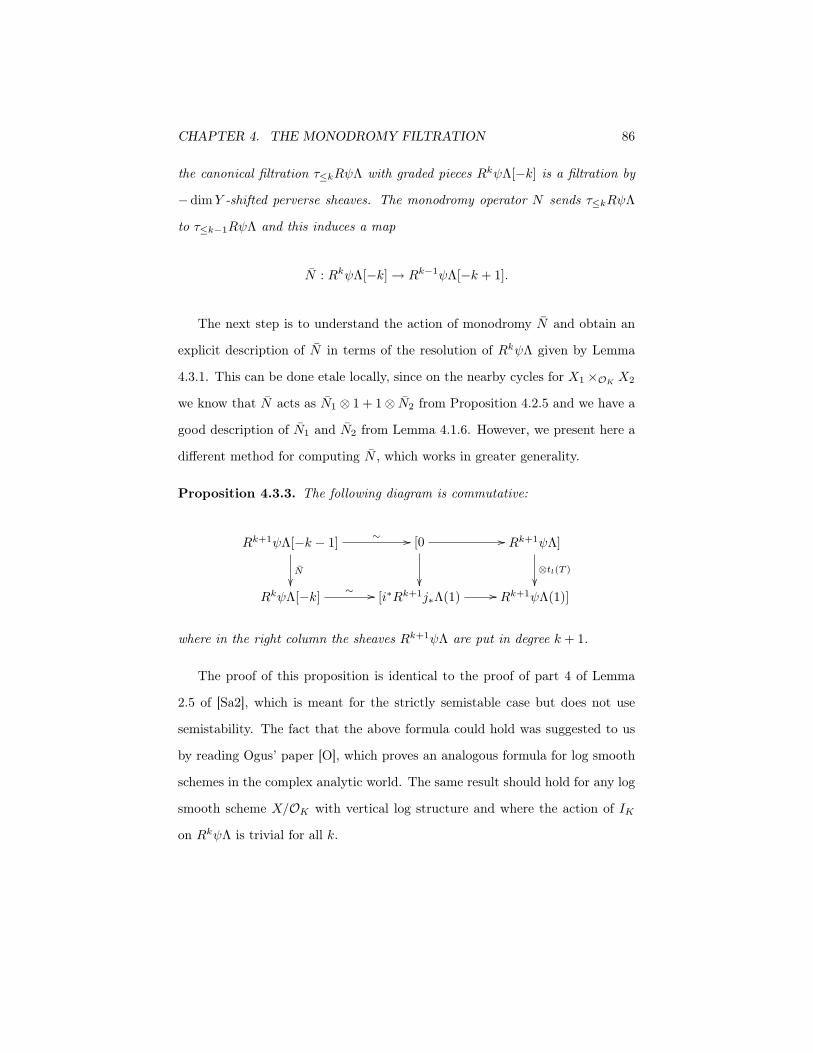
CHAPTER 4. THE MONODROMY FILTRATION 86
the canonical filtration τ≤kRψΛ with graded pieces RkψΛ[−k] is a filtration by
−dimY -shifted perverse sheaves. The monodromy operator N sends τ≤kRψΛ
to τ≤k−1RψΛ and this induces a map
N : RkψΛ[−k] → Rk−1ψΛ[−k + 1].
The next step is to understand the action of monodromy N and obtain an
explicit description of N in terms of the resolution of RkψΛ given by Lemma
4.3.1. This can be done etale locally, since on the nearby cycles for X1 ×OK X2
we know that N acts as N1 ⊗ 1 + 1⊗ N2 from Proposition 4.2.5 and we have a
good description of N1 and N2 from Lemma 4.1.6. However, we present here a
different method for computing N , which works in greater generality.
Proposition 4.3.3. The following diagram is commutative:
Rk+1ψΛ[−k − 1]
N""
∼ !! [0 !!
""
Rk+1ψΛ]
⊗tl(T )
""RkψΛ[−k] ∼ !! [i∗Rk+1j∗Λ(1) !! Rk+1ψΛ(1)]
where in the right column the sheaves Rk+1ψΛ are put in degree k + 1.
The proof of this proposition is identical to the proof of part 4 of Lemma
2.5 of [Sa2], which is meant for the strictly semistable case but does not use
semistability. The fact that the above formula could hold was suggested to us
by reading Ogus’ paper [O], which proves an analogous formula for log smooth
schemes in the complex analytic world. The same result should hold for any log
smooth scheme X/OK with vertical log structure and where the action of IK
on RkψΛ is trivial for all k.
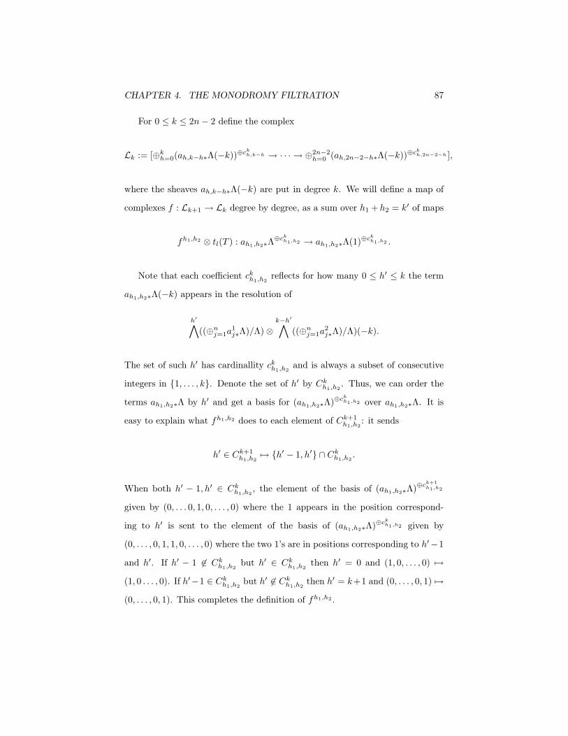
CHAPTER 4. THE MONODROMY FILTRATION 87
For 0 ≤ k ≤ 2n− 2 define the complex
Lk := [⊕kh=0(ah,k−h∗Λ(−k))⊕ck
h,k−h → · · ·→ ⊕2n−2h=0 (ah,2n−2−h∗Λ(−k))⊕ck
h,2n−2−h ],
where the sheaves ah,k−h∗Λ(−k) are put in degree k. We will define a map of
complexes f : Lk+1 → Lk degree by degree, as a sum over h1 + h2 = k′ of maps
fh1,h2 ⊗ tl(T ) : ah1,h2∗Λ⊕ck
h1,h2 → ah1,h2∗Λ(1)⊕ckh1,h2 .
Note that each coefficient ckh1,h2
reflects for how many 0 ≤ h′ ≤ k the term
ah1,h2∗Λ(−k) appears in the resolution of
h′∧((⊕n
j=1a1j∗Λ)/Λ)⊗
k−h′∧((⊕n
j=1a2j∗Λ)/Λ)(−k).
The set of such h′ has cardinallity ckh1,h2
and is always a subset of consecutive
integers in {1, . . . , k}. Denote the set of h′ by Ckh1,h2
. Thus, we can order the
terms ah1,h2∗Λ by h′ and get a basis for (ah1,h2∗Λ)⊕ckh1,h2 over ah1,h2∗Λ. It is
easy to explain what fh1,h2 does to each element of Ck+1h1,h2
: it sends
h′ ∈ Ck+1h1,h2
2→ {h′ − 1, h′} ∩ Ckh1,h2
.
When both h′ − 1, h′ ∈ Ckh1,h2
, the element of the basis of (ah1,h2∗Λ)⊕ck+1h1,h2
given by (0, . . . 0, 1, 0, . . . , 0) where the 1 appears in the position correspond-
ing to h′ is sent to the element of the basis of (ah1,h2∗Λ)⊕ckh1,h2 given by
(0, . . . , 0, 1, 1, 0, . . . , 0) where the two 1’s are in positions corresponding to h′−1
and h′. If h′ − 1 "∈ Ckh1,h2
but h′ ∈ Ckh1,h2
then h′ = 0 and (1, 0, . . . , 0) 2→
(1, 0 . . . , 0). If h′−1 ∈ Ckh1,h2
but h′ "∈ Ckh1,h2
then h′ = k+1 and (0, . . . , 0, 1) 2→
(0, . . . , 0, 1). This completes the definition of fh1,h2 .

CHAPTER 4. THE MONODROMY FILTRATION 88
Corollary 4.3.4. The following diagram is commutative
Rk+1ψΛ[−k − 1]
N""
∼ !! Lk+1
f
""RkψΛ[−k] ∼ !! Lk
,
The map f is a map of complexes, which acts degree by degree as
∑
h1+h2=k′
fh1,h2 [−k − 1]⊗ tl(T ),
where fh1,h2 : ah1,h2∗Λ⊕ck
h1,h2 → ah1,h2∗Λ⊕ck
h1,h2 was defined above.
Proof. This can be checked etale locally, using Proposition 4.2.5, which states
that N = N1 ⊗ 1 + 1 ⊗ N2 over a product X1 ×OK X2 of strictly semistable
schemes and using the fact that each of the Ni can be described as
0 !!
""
aik+1∗Λ(−(k + 1)) δ∧ !!
⊗tl(T )
""
. . . δ∧ !! ain−1∗Λ(−(k + 1))
""ai
k∗Λ(−k) δ∧ !! aik+1∗Λ(−k) δ∧ !! . . . δ∧ !! ai
n−1∗Λ(−k)
,
for i = 1, 2.
This can also be checked globally, by using Proposition 4.3.3 to replace the
leftmost column of our diagram by
0
""
!! Rk+1ψΛ
⊗tl(T )
""i∗Rk+1j∗Λ(1) !! Rk+1ψΛ(1)
,
where the left column is put in degree k. In fact, it suffices to understand the

CHAPTER 4. THE MONODROMY FILTRATION 89
map of complexes
0
""
!! Rk+1ψΛ
id
""i∗Rk+1j∗Λ !! Rk+1ψΛ
,
and check that it is compatible with the map
0 !!
fk⊗tl(T )−1
""
. . . !! ⊕2n−2h=0 (ah,2n−2−h∗Λ(−k − 1))⊕ck+1
h,2n−2−h
f2n−2⊗tl(T )−1
""⊕kh=0(ah,k−h∗Λ(−k − 1))⊕ck
h,k−h !! . . . !! ⊕2n−2h=0 (ah,2n−2−h∗Λ(−k − 1))⊕ck
h,2n−2−h
.
Let K = Cone(f ⊗ tl(T )−1 : Lk+1 → Lk(−1)). The triangle
RkψΛ[−k − 1] !! i∗Rk+1j∗Λ[−k − 1] !! Rk+1ψΛ[−k − 1]N⊗tl(T )−1
!! RkψΛ[−k]
is distinguished. It suffices to see that we can define a map g : i∗Rk+1j∗Λ[−k] →
K which makes the first two squares of the following diagram commute:
RkψΛ[−k − 1] !!
θk[−1]
""
i∗Rk+1j∗Λ[−k − 1] !!
g[−1]
""
Rk+1ψΛ[−k − 1]N⊗tl(T )−1
!!
θk+1
""
RkψΛ[−k]
θk
""Lk(−1)[−1] !! K[−1] !! Lk+1
f⊗tl(T )−1!! Lk(−1)
If the middle square is commutative, then there must exist θ′ : RkψΛ[−k−1] →
Lk(−1)[−1] making the diagram a morphism of distinguished triangles. Then
θ′ would make the first square commutative, so θ′ and θk[−1] coincide once they
are pushed forward to K[−1]. However,
Hom(RkψΛ[−k − 1],Lk+1[−1]) * Hom(RkψΛ[−k], Rk+1ψΛ[−k − 1]) = 0,

CHAPTER 4. THE MONODROMY FILTRATION 90
so the Hom exact sequence associated to the bottom distinguished triangle im-
plies that θ′ = θk[−1]. The diagram above is a morphism of distinguished
triangles with θk[−1] as the leftmost morphism. This tells us that the third
triangle in the diagram is also commutative, which is what we wanted to prove.
We can compute i∗Rk+1j∗Λ using the log structure on X:
i∗Rk+1j∗Λ(k+1) * ∧k+1((n⊕
j=1
a1j∗Λ⊕
n⊕
j=1
a2j∗Λ)/(1, . . . 1, 0, . . . 0)−(0, . . . , 0, 1, . . . , 1)).
Here we have used, again, the formula i∗Rkj∗Λ(k) * ∧k(Mgp)⊗Λ, which follows
from Proposition 2.0.2 of [Na]. We can also compute K explicitly, since we have
an explicit description of each fk′,h1,h2 . The first non-zero term of K appears
in degree k and it is isomorphic to
k∑
h=0
ah,k−h∗Λ.
There is a natural map of complexes i∗Rk+1j∗Λ[−k] → K, which sends
aJ1,J2∗Λ →⊕
J′1⊃J1,#J′1=#J1+1
aJ′1,J2∗Λ⊕⊕
J′2⊃J2,#J′2=#J2+1
aJ1,J ′2∗Λ,
when J1, J2 are both non-empty. The map sends
aJ1,∅∗Λ →⊕
#J′2=1
aJ1,J ′2∗Λ and a∅,J2∗Λ →⊕
#J′1=1
aJ′1,J2∗Λ.
It is easy to see that the above map is well-defined on i∗Rk+1j∗Λ[−k] and that it
is indeed a map of complexes. It remains to see that the above map of complexes
i∗Rk+1j∗Λ[−k] → K makes the first two squares of the diagram commute. This
is tedious, but straightforward to verify.
Remark 4.3.5. Another way of proving the above corollary is to notice that

CHAPTER 4. THE MONODROMY FILTRATION 91
Proposition 4.3.3 shows that the map
N : Rk+1ψΛ[−k − 1] → RkψΛ[−k]
is given by the cup product with the map γ ⊗ tl(T ) : Mgprel(−k− 1) → Λ(−k)[1]
where γ : Mgprel → Λ[1] is the map corresponding to the class of the extension
0 → Λ → Mgp → Mgprel → 0
of sheaves of Λ-modules on Y . Locally, X is etale over a product of strictly
semistable schemes X1×OK X2 and the extension Mgp is a Baire sum of exten-
sions
0 → Λ → Mgp1 → Mgp
1,rel → 0 and
0 → Λ → Mgp2 → Mgp
2,rel → 0,
which correspond to the log structures of X1 and X2 and which by Proposition
4.3.3 determine the maps N1 and N2. The Baire sum of extensions translates
into N = N1 ⊗ 1 + 1⊗ N2 locally on Y . However, it is straightforward to check
locally on Y that the map f : Lk → Lk+1 is the same as N1⊗1+1⊗N2. Thus, f
and N are maps of perverse sheaves on Y which agree locally on Y , which means
that f and N agree globally. This proves the corollary without appealing to
Proposition 4.3.3. (In fact, it suggests an alternate proof of Proposition 4.3.3.)
The following results, Lemma 4.3.6 to Corollary 4.3.10, are just generaliza-
tions of Lemma 4.2.8 to Corollary 4.2.13. We merely sketch their proofs here.
Lemma 4.3.6. The map N : RkψΛ[−k] → Rk−1ψΛ[−k + 1] has kernel
Pk *[ak,k∗Λ(−k) ∧δ→ ak,k+1∗Λ(−k)⊕ ak+1,k∗Λ(−k) → · · · ∧δ→ an−1,n−1∗Λ(−k)
],

CHAPTER 4. THE MONODROMY FILTRATION 92
where the first term is put in degree 2k and cokernel
Rk *[⊕k−1
j=0aj,k−1−j∗Λ(−(k − 1)) → · · ·→ ak−1,k−1∗Λ((−(k − 1))],
where the first term is put in degree k − 1.
Proof. The proof is identical to the proof of Lemma 4.2.8, since by Proposition
4.3.3 we have a description of N as a degree by degree map
f : Lk → Lk−1.
Corollary 4.3.7. The filtration of RψΛ by τ≤kRψΛ induces a filtration on
kerN . The first graded piece of this filtration Gr1 kerN is R0ψΛ. The graded
piece Grk+1 kerN of this filtration is Pk.
Proof. This can be proved the same way as Corollary 4.2.9. The only tricky part
is seeing that we can identify a graded piece of ker N with a graded piece of
kerN . In other words, we want to show that for N : RkψΛ[−k] → Rk−1ψΛ[−k+
1] and x ∈ ker N we can find a lift x ∈ τ≤kRψΛ of x such that x ∈ kerN . As
in the proof of Corollary 4.2.9, we can define a map Pk → Rk−1 sending x to
the image of Nx in Rk−1, which turns out to be independent of the lift x. We
want to see that this map vanishes but in fact any map Pk → Rk−1 vanishes.
Note that
ah1,h2∗Λ[−h1 − h2] * ⊕#S=h1+1,#T=h2+1aS,T∗Λ[−h1 − h2].
The scheme YS,T is smooth of pure dimension dimY − h1 − h2 and so it is a
disjoint union of its irreducible (connected) components which are smooth of
pure dimension dimY − h1 − h2. Thus, each aS,T∗Λ[−h1 − h2] is the direct

CHAPTER 4. THE MONODROMY FILTRATION 93
sum of the pushforwards of the −dimY -shifted perverse sheaves Λ[−h1 − h2]
on the irreducible components of YS,T . Thus, we have a decomposition of
ah1,h2∗Λ[−h1−h2] in terms of simple objects in the category of −dimY -shifted
perverse sheaves. It is easy to check that Pk and Rk−j for k ≥ j ≥ 1 have no
simple factors in common, so any map Pk → Rk−j must vanish.
Remark 4.3.8. The same techniques used in Section 4.2 apply in order to com-
pletely determine the graded pieces of (kerN j/ kerN j−1)/(im N ∩ kerN j) in-
duced by the filtration of RψΛ by τ≤kRψΛ. The only tricky part is seeing that
we can also identify the kth graded piece of imN with
im(N : Rk+1ψΛ[−k − 1] → RkψΛ[−k]),
but this can be proved in the same way as the corresponding statement about
the kernels of N and N . We get a complete description of the graded pieces of
(kerN j/ kerN j−1)/im N .
Lemma 4.3.9. For 1 ≤ j ≤ 2n− 2, the filtration of RψΛ by τ≤kRψΛ induces
a filtration on (kerN j/ kerN j−1)/imN . For 0 ≤ k ≤ n− 1− j−12 , the (k +1)-st
graded piece of this filtration is isomorphic to
⊕ji=1ak+i−1,k+j−i∗Λ(−(k + j − 1))[−2k − j + 1].
As in Corollary 4.2.12, since each graded piece of the filtration is pure of weight
j − 1, the filtration is in fact a direct sum.
Let
GrqGrpRψΛ = (kerNp ∩ imNq)/(kerNp−1 ∩ imNq) + (kerNp ∩ imNq+1).

CHAPTER 4. THE MONODROMY FILTRATION 94
The monodromy filtration MrRψΛ has graded pieces GrMr RψΛ isomorphic to
GrMr RψΛ *
⊕
p−q=r
GrqGrpRψΛ,
and if we understand the cohomology of YF with coefficients in each GrqGrpRψΛ
we can compute the cohomology of YF with respect to RψΛ. The next result
tells us how to compute Hm(YF,GrqGrpRψΛ).
Corollary 4.3.10. There is a direct sum decomposition
Hm(YF,GrqGrpRψΛ) *⊕
k≥0
p+q⊕
i=1
Hm(YF, ak+i−1,k+p+q−i∗Λ(−(k+p−1))[−2k−p−q+1])
compatible with the action of GF. This can be rewritten as
Hm(YF,GrqGrpRψΛ) *⊕
k≥0
p+q⊕
i=1
Hm−2k−p−q+1(Y (k+i−1,k+p+q−i)F ,Λ(−(k+p−1))).
Remark 4.3.11. The isomorphism above is functorial with respect to etale mor-
phisms which preserve the stratification by YS,T with S, T ⊂ {1, . . . , n}. The
reason for this is that etale morphisms preserve both the kernel and the image
filtration of N as well as the canonical filtration τ≤kRψΛ.

Chapter 5
The cohomology of closed
strata
In tthis chapter we go back to working with the Iwahori level Shimura variety
XU/OK as well as with the Shimura variety XU0/OK with no level structure at
p1 and p2, both corresponding to the unitary group G. Recall that K = Fp1 *
Fp2 , with ring of integers OK , uniformizer π and residue field F.
5.1 Igusa varieties
Let q = p[F:Fp]. Fix 0 ≤ h1, h2 ≤ n − 1 and consider the stratum X(h1,h2)U0
of
the Shimura variety XU0 . Choose a compatible one-dimensional formal OF,p1 =
OK-module Σ1, of height n− h1 and also a compatible one-dimensional formal
OF,p2 * OK-module Σ2 of height n − h2. Giving Σ1 and Σ2 is equivalent to
giving a triple (Σ, λΣ, iΣ) where:
• Σ is a Barsotti-Tate group over F.
• λΣ : Σ → Σ∨ is a polarization.
95

CHAPTER 5. THE COHOMOLOGY OF CLOSED STRATA 96
• iΣ : OF → End(Σ)⊗Z Z(p) such that (Σ, iΣ) is compatible.
Note that (Σ[p∞i ])0 * Σi for i = 1, 2 while (Σ[p∞i ])et * (K/OK)n−hi .
Assume that the level U0 corresponds to the vector -m = (0, 0, m3, . . . ,mr).
Let
-m′ = ((m0i , m
eti )i=1,2, m3, . . . ,mr),
with the same entries m3, . . . ,mr as -m. The Igusa variety Ig(h1,h2)
Up, %m′ over X(h1,h2)U0
×F
F is defined to be the moduli space of the set of the following isomorphisms of
finite flat group schemes for i = 1, 2:
• α0i : Σi[p
m0i
i ] ∼→ G0i [pm0
ii ], which extends etale locally to any (m0
i )′ ≥ m0i
and
• αeti : (p−met
ii OF,pi/OF,pi)hi
∼→ Geti [pmet
ii ].
In other words, if S/F is a scheme, then an S-point of the Igusa variety Ig(h1,h2)Up,%m
corresponds to a tuple
(A, λ, i, ηp, (α0i )i=1,2, (αet
i )i=1,2, (αi)i≥3),
where
• A is an abelian scheme over S with GA,i = A[p∞i ];
• λ : A → A∨ is a prime-to-p polarization;
• i : OF ↪→ End(A) ⊗Z Z(p) such that (A, i) is compatible and λ ◦ i(f) =
i(f∗)∨ ◦ λ,∀f ∈ OF ;
• ηp : V ⊗Q A∞,p → V pA is a π1(S, s)-invariant Up-orbit of isomorphisms
of F ⊗Q A∞,p-modules, sending the standard pairing on V ⊗Q A∞,p to an
(A∞,p)×-multiple of the λ-Weil pairing;

CHAPTER 5. THE COHOMOLOGY OF CLOSED STRATA 97
• α0i : Σ0[pm0
ii ] ∼→ G0
A,i[pm0
ii ] is an OK-equivariant isomorphism of finite flat
group schemes which extends to any higher level (m′)0i ≥ m0i , for i = 1, 2
and some integer (m′)0i ;
• αeti : Σet[pmet
ii ] ∼→ Get
A,i[pmet
ii ] is an OK-equivariant isomorphism of etale
group schemes, for i = 1, 2;
• αi : Σ[pmii ] ∼→ GA,i[pmi
i ] is an OF,pi-equivariant isomorphism of etale group
schemes, for 3 ≤ i ≤ r.
Two such tuples are considered equivalent if there exists a prime-to-p isogeny
f : A → A′ taking (A, λ, i, ηp, α0i , α
eti , αi) to (A′, γλ′, i′, ηp′ , α0′
i , αet′i , α′i) for
γ ∈ Z×(p).
The Igusa varieties Ig(h1,h2)Up,%m form an inverse system which has an action of
G(A∞,p) inherited from the action on X(h1,h2)U0
. Let
J (h1,h2)(Qp) = Q×p ×D×K,n−h1
×GLh1(K)×D×K,n−h2
×GLh2(K)×r∏
i=3
GLn(Fpi),
which is the group of quasi-self-isogenies of (Σ, λΣ, iΣ) (to compute J (h1,h2)(Qp)
we use the duality induced from the polarization). The automorphisms of
(Σ, λΣ, iΣ) have an action on the right on Ig(h1,h2)Up,%m . This can be extended to an
action of a certain submonoid of J (h1,h2)(Qp) on the inverse system of Ig(h1,h2)Up,%m
and furthermore to an action of the entire group J (h1,h2)(Qp) on the directed
system Hjc (Ig(h1,h2)
Up,%m ,Lξ). For a definition of this action, see section 5 of [Sh1]
and section 4 of [Man].
We also define an Iwahori-Igusa variety of the first kind I(h1,h2)U /XU0 as the
moduli space of chains of isogenies for i = 1, 2
Geti = Gi,0 → Gi,1 → · · ·→ Gi,hi = Get
i /Geti [pi]

CHAPTER 5. THE COHOMOLOGY OF CLOSED STRATA 98
of etale Barsotti-Tate OK-modules, each isogeny having degree #F and with
composite equal to the natural map Geti → Get
i /Geti [pi]. Then I(h1,h2)
U is finite
etale over X(h1,h2)U0
and naturally inherits the action of G(A∞,p). Moreover, for
m01 = m0
2 = 0 and met1 = met
2 = 1 we know that Ig(h1,h2)Up,%m′ /I(h1,h2)
U ×F F is finite
etale and Galois with Galois group Bh1(F)×Bh2(F). (Here Bhi(F) ⊆ GLhi(F)
is the Borel subgroup.)
Lemma 5.1.1. For S, T ⊂ {1, . . . , n} with #S = n − h1,#T = n − h2 there
exists a finite map of X(h1,h2)U0
-schemes
ϕ : Y 0U,S,T → I(h1,h2)
U
which is bijective on the sets of geometric points.
Proof. The proof is a straightforward generalization of the proof of Lemma 4.1
of [TY].
Recall that for a given -m with m1 = m2 = 0 we take
U = Up × Up1,p2p (-m)× Iwn,p1 × Iwn,p2 × Z×p ,
restricting ourselves to Iwahori level structure at p1 and p2. Now we let the
level away from p vary. Define
Hjc (Y 0
Iw(%m),S,T ,Lξ) = lim−→Up
Hjc (Y 0
U,S,T ,Lξ),
Hj(YIw(%m),S,T ,Lξ) = lim−→Up
Hj(YU,S,T ,Lξ),
Hjc (I(h1,h2)
Iw(%m) ,Lξ) = lim−→Up
Hjc (I(h1,h2)
U ×F F,Lξ).

CHAPTER 5. THE COHOMOLOGY OF CLOSED STRATA 99
Without restriction on -m′ we can define
Hjc (Ig(h1,h2),Lξ) = lim−→
Up,%m′Hj
c (Ig(h1,h2)
Up, %m′ ,Lξ)
For m01 = m0
2 = 0, the Igusa variety Ig(h1,h2)Up,%m′ is defined over F. If in addition,
met1 = met
2 = 1 then Ig(h1,h2)Up,%m′ (over F) is a Galois cover of I(h1,h2)
U with Galois
group Bh1(F)×Bh2(F).
Corollary 5.1.2. Let -m′ = (0, 0, 1, 1, m3, . . . ,mr). For every S, T ⊆ {1, . . . n−
1} with #S = n− h1,#T = n− h2 and j ∈ Z≥0 we have the following isomor-
phism
Hjc (Y 0
U,S,T ×F F,Lξ) * Hjc (I(h1,h2)
Up,%m′ ×F F,Lξ)Bh1 (F)×Bh2 (F).
By taking a direct limit over Up and over -m = (0, 0, m3, . . . ,mr) and con-
sidering the definitions of the Igusa varieties, we get an isomorphism
Hjc (Y 0
Iw(%m),S,T,Lξ) * Hj
c (Ig(h1,h2),Lξ)Up1p2
p (%m)×Iwh1,p1×O×DK,n−h1
×Iwh2,p2×O×DK,n−h2 .
Taking a limit over general -m′ satisfying m01 = m0
2 = 0 we define
Hjc (Ig(h1,h2)
0 ,Lξ) := lim−→Up,%m′
m01=m0
2=0
Hjc (Ig(h1,h2)
Up,%m′ ×F F,Lξ).
Then the above isomorphism becomes
Hjc (Y 0
Iw(%m),S,T,Lξ) * Hj
c (Ig(h1,h2)0 ,Lξ)Up1p2
p ×Iwh1,p1×Iwh2,p2 .
Proposition 5.1.3. The action of FrobF on Hjc (Ig(h1,h2)
0 ,Lξ) coincides with
the action of (1, (p−[F:Fp],−1, 1,−1, 1, 1)) ∈ G(A∞,p)× J (h1,h2)(Qp).
Proof. Let Fr : x 2→ xp be the absolute Frobenius on Fp and let f = [F : Fp].

CHAPTER 5. THE COHOMOLOGY OF CLOSED STRATA 100
To compute the action of the geometric Frobenius FrobF on Hjc (Ig(h1,h2)
0 ,Lξ)
we notice that the absolute Frobenius acts on each Hjc (Ig(h1,h2)
Up,%m ×F F,Lξ) as
(Fr∗)f × (Frob∗F)−1. However, the absolute Frobenius acts trivially on etale
cohomology, so the action of FrobF coincides with the action induced from
(Fr∗)f : Ig(h1,h2)Up,%m′ → Ig(h1,h2)
Up,%m′
We claim that (Fr∗)f acts the same as the element (1, p−[F:Fp],−1, 1,−1, 1, 1) of
G(A∞,p)×Q×p /Z×p × Z×GLh1(K)× Z×GLh2(K)×r∏
i=3
GLn(Fpi),
where the two copies of Z are identified with D×K,n−hi
/O×DK,n−hifor i = 1, 2 via
the valuation of the determinant. To verify this claim, we will use the explicit
description of the action of a submonoid J (h1,h2)(Qp) on the inverse system of
Igusa varieties Ig(h1,h2)Up,%m′ found in [Man] which generalizes that on page 122 of
[HT]. First, it is easy to see that
(Fr∗)f : (A, λ, i, ηp, α0i , α
eti , αi) 2→ (A(q), λ(q), i(q), (ηp)(q), (α0
i )(q), (αet
i )(q), α(q)i )
where F f : A → A(q) is the natural map and the structures of A(q) are inherited
from the structures of A via F f .
On the other hand, the element j = (1, p−[F:Fp],−1, 1,−1, 1, 1) acts via a
quasi-isogeny of Σ. One can check that the inverse of the quasi-isogeny defined
by j is j−1 : Σ → Σ(q), which is a genuine isogeny. If we were working with
points of Ig(h1,h2) (which are compatible systems of points of Ig(h1,h2)Up,%m′ for all
Up and -m′) then j should act by precomposing all the isomorphism α0i , α
eti for
i = 1, 2 and αi for 3 ≤ i ≤ r. Since j|A[p∞i ]et = 1 for i = 1, 2 and j|A[p∞i ] = 1 for
3 ≤ i ≤ r the isomorphisms αeti and αi stay the same. However, α0
i ◦j is now only
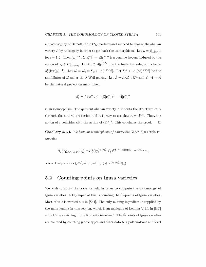
CHAPTER 5. THE COHOMOLOGY OF CLOSED STRATA 101
a quasi-isogeny of Barsotti-Tate OK-modules and we need to change the abelian
variety A by an isogeny in order to get back the isomorphisms. Let ji = j|Σ[p∞i ]0
for i = 1, 2. Then (ji)−1 : Σ[p∞i ]0 → Σ[p∞i ]0 is a genuine isogeny induced by the
action of πi ∈ D×K,n−hi
. Let Ki ⊂ A[p[F:Fp]i ] be the finite flat subgroup scheme
α0i (ker(ji)−1). Let K = K1 ⊕ K2 ⊂ A[u[F:Fp]]. Let K⊥ ⊂ A[(uc)[F:Fp]] be the
annihilator of K under the λ-Weil pairing. Let A = A/K ⊕ K⊥ and f : A → A
be the natural projection map. Then
β0i = f ◦ α0
i ◦ ji : (Σ[p∞i ])0 → A[p∞i ]0
is an isomorphism. The quotient abelian variety A inherits the structures of A
through the natural projection and it is easy to see that A = A(q). Thus, the
action of j coincides with the action of (Fr∗)f . This concludes the proof.
Corollary 5.1.4. We have an isomorphism of admissible G(A∞,p)× (FrobF)Z-
modules
Hjc (Y 0
Iw(%m),S,T ,Lξ) * Hjc (Ig(h1,h2)
0 ,Lξ)Up1p2p (%m)×Iwh1,p1×Iwh2,p2 ,
where FrobF acts as (p−f ,−1, 1,−1, 1, 1) ∈ J (h1,h2)(Qp).
5.2 Counting points on Igusa varieties
We wish to apply the trace formula in order to compute the cohomology of
Igusa varieties. A key input of this is counting the F−points of Igusa varieties.
Most of this is worked out in [Sh1]. The only missing ingredient is supplied by
the main lemma in this section, which is an analogue of Lemma V.4.1 in [HT]
and of “the vanishing of the Kottwitz invariant”. The F-points of Igusa varieties
are counted by counting p-adic types and other data (e.g polarizations and level

CHAPTER 5. THE COHOMOLOGY OF CLOSED STRATA 102
structure). We can keep track of p-adic types via Honda-Tate theory; we need
to check that these p-adic types actually correspond to a point on one of our
Igusa varieties.
A simple p-adic type over F is a triple (M, η, κ) where
• M is a CM field, with P being the set of places of M over p,
• η =∑
x∈P ηxx is an element of Q[P], the Q-vector space with basis P,
• κ : F → M is a Q-algebra homomorphism
such that ηx ≥ 0 for all x ∈ P and η + c∗η =∑
x∈P x(p) · x in Q[P], where
p =∏
x∈P xx(p). Here c is the complex conjugation on M and
c∗ : Q[P] → Q[P]
is the Q-linear map satisfying x 2→ xc. See page 24 of [Sh1] for the general
definition of a p-adic type. As in [Sh1], we will drop κ from the notation, since
it is well understood as the F -algebra structure map of M .
We can recover a simple p-adic type from the following data:
• a CM field M/F ;
• for i = 1, 2 places pi of M above pi such that [Mpi: Fpi ]n = [M : F ](n−hi)
and such that there is no intermediate field F ⊂ N ⊂ M with pi|N both
inert in M .
Using this data, we can define a simple p-adic type (M, η), where the coefficients
of η at places above u are non-zero only for p1 and p2. The abelian variety A/F
corresponding to (M, η) will have an action of M via i : M ↪→ End0(A). By
Honda-Tate theory, the pair (A, i) will also satisfy
• M is the center of End0F (A),

CHAPTER 5. THE COHOMOLOGY OF CLOSED STRATA 103
• A[p∞i ]0 = A[p∞i ] has dimension 1 and A[p∞i ]e has height hi for i = 1, 2,
• and A[p∞i ] is ind-etale for i > 2.
Lemma 5.2.1. Let M/F be a CM field as above. Let A/F be the corresponding
abelian variety equipped with i : M ↪→ End0(A). Then we can find
• a polarization λ0 : A → A∨ for which the Rosati involution induces c on
i(M), and
• a finitely-generated M -module W0 together with a non-degenerate Hermi-
tian pairing
〈·, ·〉0 : W0 ×W0 → Q
such that the following are satisfied:
• there is an isomorphism of M ⊗ A∞,p-modules
W0 ⊗ A∞,p ∼→ V pA
which takes 〈·, ·〉0 to an (A∞,p)×-multiple of the λ0 -Weil pairing on V pA,
and
• there is an isomorphism of F ⊗Q R-modules
W0 ⊗Q R ∼→ V ⊗Q R
which takes 〈·, ·〉0 to an R×-multiple of our standard pairing 〈·, ·〉 on V ⊗Q
R.
Proof. By Lemma 9.2 of [Ko1] there is a polarization λ0 : A → A∨ such that
the λ0-Rosati involution preserves M and acts on it as c. The next step is to
show that, up to isogeny, we can lift (A, i,λ0) from F to OKac . Using the results

CHAPTER 5. THE COHOMOLOGY OF CLOSED STRATA 104
of [Tat] we can find some lift of A to an abelian scheme A/OKac in such a way
that i lifts to an action i of M on A. As in the proof of Lemma V.4.1 of [HT]
we find a polarization λ of A which reduces to λ. However, we want to be more
specific about choosing our lift A. Indeed, for any lift, LieA ⊗OacK
Kac is an
F ⊗Kac * (Kac)Hom(F,Kac)-module, so we have a decomposition
LieA⊗OKac Kac *⊕
τ∈Hom(F,Kac)
(LieA)τ .
Let Hom(F,Kac)+ be the the set of places τ ∈ Hom(F,Kac) which induce the
place u of E. We want to make sure that the set of places τ ∈ Hom(F,Kac)+
for which (LieA)τ is non-trivial has exactly two elements τ ′1 and τ ′2 which differ
by our distinguished element σ ∈ Gal(F/Q), i.e.
τ ′2 = τ ′1 ◦ σ.
In order to ensure this, we need to go through Tate’s original argument for
constructing lifts A of A.
First, let Φ =∑
τ∈Hom(M,Kac) Φτ · τ with the Φτ non-negative integers sat-
isfying Φτ + Φτc = n. For any such Φ, we can construct an abelian variety AΦ
over OKac such that
LieAΦ ⊗OKac Kac *⊕
τ∈Hom(F,Kac)
(LieAΦ)τ
satisfies dim(LieAΦ)τ = Φτ . This is done as in Lemma 4 of [Tat], which proves
the case n = 1. We pick any τ ′i ∈ Hom(F,Kac) inducing the places pi of F for i =
1, 2 such that τ ′2 = τ ′1 ◦σ. We lift the τ ′i to elements τi ∈ Hom(M,Kac) inducing
pi. We let Φτi = 1 and Φτ = 0 for any other τ ∈ Hom(M,Kac)+. For τ "∈
Hom(M, Kac)+ we define Φτ = n−Φτc . This determines Φ ∈ Q[Hom(M, Kac)]

CHAPTER 5. THE COHOMOLOGY OF CLOSED STRATA 105
entirely. This Φ is not quite a p-adic type for M , however it is easy to associate
a p-adic type to it: we define η =∑
x|p ηx · x by
ηx =ex/p · [M : F ]n · [Mx : Qp]
·∑
Φτ ,
where the sum is over embeddings τ ∈ Hom(M,Kac) which induce the place
x of M . By Honda-Tate theory, the reduction of the abelian scheme AΦ/OKac
associated to Φ has p-adic type η. Indeed, the height of the p-divisible group
at x of the reduction of AΦ is n·[Mx:Qp][M :F ] (see Proposition 8.4 of [Sh1] together
with an expression of dimA in terms of M). The dimension of the p-divisible
group at x of the reduction is∑
Φτ , where we’re summing over all embeddings
τ which induce x.
Now we set A = AΦ. It remains to check that A/OKac has special fiber
isogenous to A/F and this follows from the fact that the reductions of A and A
are both associated to the same p-adic type η. Indeed, it suffices to verify this
for places x above u. We have
ηx = 0 = ex/p ·dimA[x∞]
heightA[x∞]
for all places x "= pi for i = 1, 2. When x = pi we have
ηx = ex/p·[M : F ]
[Mx : Fpi ] · n · [Fpi : Qp]= ex/p·
1(n− hi) · [Fpi : Qp]
= ex/p·dimA[x∞]
heightA[x∞].
Therefore, the p-adic type associated to A is also η.
There are exactly two distinct embeddings τ ′1, τ′2 ∈ Hom(F,Kac)+ such that
(LieA)τ "= (0) only when τ = τ ′1 or τ ′2. Moreover, these embeddings are related
by τ ′2 = τ ′1 ◦ σ. Therefore, we can find an embedding κ : Kac ↪→ C such that

CHAPTER 5. THE COHOMOLOGY OF CLOSED STRATA 106
κ ◦ τ ′i = τi for i = 1, 2. We set
W0 = H1((A×Spec OKac ,κ Spec C)(C), Q).
From here on, the proof proceeds as the proof of Lemma V.4.1 of [HT].
5.3 Vanishing of cohomology
Let Π1 be an automorphic representation of GL1(AE)×GLn(AF ) and assume
that Π1 is cuspidal. Let 6 : A×E/E× → C be any Hecke character such that
6|A×/Q× is the composite of ArtQ and the natural surjective character WQ !
Gal(E/Q) ∼→ {±1}.
Also assume that Π1 and F satisfy
• Π1 * Π1 ◦ θ.
• Π1∞ is generic and Ξ1-cohomological, for some irreducible algebraic repre-
sentation Ξ1 of Gn(C), which is the image of ιlξ under the base change
from GC to Gn,C.
• RamF/Q ∪ RamQ(6) ∪ RamQ(Π) ⊂ SplF/F2,Q.
Let S = Sfin ∪ {∞} be a finite set of places of F , which contains the places
of F above places of Q which are ramified in F and the places where Π is
ramified. For l "= p, let ι : Ql∼→ C and let πp ∈ Irrl(G(Qp)) be such that
BC(ιlπp) * Πp. If we write Π1 = ψ⊗Π0 and πp = πp,0⊗πp1 ⊗πp2 ⊗ (⊗ri=3πpi)
then ιlπp,0 * ψu and ιlπpi * Π0pi
for all 1 ≤ i ≤ r. Under the identification
Fp1 * Fp2 , assume that Π0p1* Π0
p2(this condition will be satisfied in all our
applications, since we will choose Π0 to be the base change of some cuspidal
automorphic representation Π of GLn(AF1E)).

CHAPTER 5. THE COHOMOLOGY OF CLOSED STRATA 107
Define the following elements of Groth(G(A∞,p)×J (h1,h2)(Qp)) (the Grothendieck
group of admissible representations):
[Hc(Ig(h1,h2),Lξ)] =∑
i
(−1)h1+h2−iHic(Ig
(h1,h2),Lξ)
If R ∈ Groth(G(AS) × G′), we can write R =∑
πS⊗ρ n(πS ⊗ ρ)[πS][ρ],
where πS and ρ run over Irrl(G(AS)) and Irrl(G′) respectively. We define
R{πS} :=∑
ρ
n(πS ⊗ ρ)[ρ], R[πS] :=∑
ρ
n(πS ⊗ ρ)[πS][ρ].
Also define
R{Π1,S} :=∑
πS
{πS}, R[Π1,S] :=∑
πS
R[πS],
where each sum runs over πS ∈ Irrurl (G(AS)) such that BC(ιlπS) * ΠS.
Let Red(h1,h2)n (πp) be the morphism from Groth(G(Qp)) to Groth(J (h1,h2)(Qp))
defined by
(−1)h1+h2πp,0 ⊗ Redn−h1,h1(πp1)⊗ Redn−h2,h2(πp2)⊗ (⊗i>2πpi),
where
Redn−h,h : Groth(GLn(K)) → Groth(D×K, 1
n−h×GLh(K))
is obtained by composing the normalized Jacquet functor
J : Groth(GLn(K)) → Groth(GLn−h(K)×GLh(K))
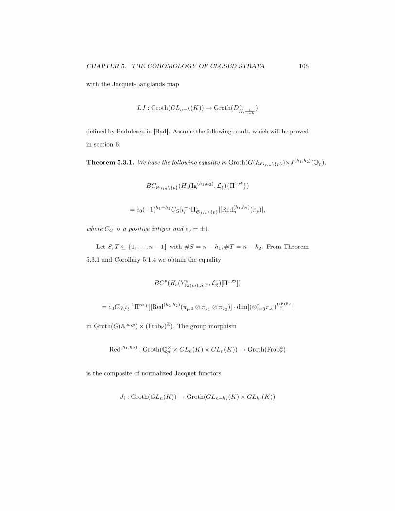
CHAPTER 5. THE COHOMOLOGY OF CLOSED STRATA 108
with the Jacquet-Langlands map
LJ : Groth(GLn−h(K)) → Groth(D×K, 1
n−h)
defined by Badulescu in [Bad]. Assume the following result, which will be proved
in section 6:
Theorem 5.3.1. We have the following equality in Groth(G(ASfin\{p})×J (h1,h2)(Qp):
BCSfin\{p}(Hc(Ig(h1,h2),Lξ){Π1,S})
= e0(−1)h1+h2CG[ι−1l Π1
Sfin\{p}][Red(h1,h2)n (πp)],
where CG is a positive integer and e0 = ±1.
Let S, T ⊆ {1, . . . , n− 1} with #S = n− h1,#T = n− h2. From Theorem
5.3.1 and Corollary 5.1.4 we obtain the equality
BCp(Hc(Y 0Iw(m),S,T ,Lξ)[Π1,S])
= e0CG[ι−1l Π∞,p][Red(h1,h2)(πp,0 ⊗ πp1 ⊗ πp2)] · dim[(⊗r
i=3πpi)Up1p2
p ]
in Groth(G(A∞,p)× (FrobF)Z). The group morphism
Red(h1,h2) : Groth(Q×p ×GLn(K)×GLn(K)) → Groth(FrobZF)
is the composite of normalized Jacquet functors
Ji : Groth(GLn(K)) → Groth(GLn−hi(K)×GLhi(K))
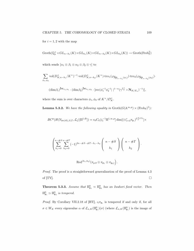
CHAPTER 5. THE COHOMOLOGY OF CLOSED STRATA 109
for i = 1, 2 with the map
Groth(Q×p ×GLn−h1(K)×GLh1(K)×GLn−h2(K)×GLh2(K)) → Groth(FrobZF)
which sends [α1 ⊗ β1 ⊗ α2 ⊗ β2 ⊗ γ] to
∑
φ1,φ2
vol(D×K,n−h1
/K×)−1·vol(D×K,n−h2
/K×)·trα1(ϕSpn−h1(φ1)
)·trα2(ϕSpn−h2(φ2)
)·
·(dimβ1)Iwh1,p1 · (dimβ2)Iwh1,p2 · [rec(φ−11 φ−1
2 | |1−n(γZ×p ◦NK/Eu)−1)],
where the sum is over characters φ1, φ2 of K×/O×K .
Lemma 5.3.2. We have the following equality in Groth(G(A∞,p)× (FrobF)Z):
BCp(H(YIw(%m),S,T ,Lξ)[Π1,S]) = e0CG[ι−1l Π1,∞,p] dim[(⊗r
i=3πpi)Up1p2
p ]×
n−#S∑
h1=0
n−#T∑
h2=0
(−1)2n−#S−#T−h1−h2
n−#S
h1
n−#T
h2
·
Red(h1,h2)(πp,0 ⊗ πp1 ⊗ πp2)
).
Proof. The proof is a straightforward generalization of the proof of Lemma 4.3
of [TY].
Theorem 5.3.3. Assume that Π0p1* Π0
p2has an Iwahori fixed vector. Then
Π0p1* Π0
p2is tempered.
Proof. By Corollary VII.2.18 of [HT], ιlπpi is tempered if and only if, for all
σ ∈ WK every eigenvalue α of Ln,K(Π0pi
)(σ) (where Ln,K(Π0pi
) is the image of

CHAPTER 5. THE COHOMOLOGY OF CLOSED STRATA 110
Π0pi
under the local Langlands correspondence, normalized as in [Sh3]) satisfies
|ιlα|2 ∈ qZ.
We shall first use a standard argument to show that we can always ensure that
|ιlα|2 ∈ q12 Z
and then we will use a classification of irreducible, generic, ι-preunitary repre-
sentations of GLn(K) together with the cohomology of Igusa varieties to show
the full result.
The space Hk(X,Lξ) decomposes as a G(A∞)-module as
Hk(X,Lξ) =⊕
π∞
π∞ ⊗Rkξ,l(π
∞),
where π∞ runs over Irrl(G(A∞)) and Rkξ.l(π
∞) is a finite-dimensional Gal(F /F )-
representation. Define the Gal(F /F )-representation
Rkl (Π1) =
∑
π∞
Rkξ,l(π
∞),
where the sum is over the π∞ ∈ Irrl(G(A∞)) which are cohomological, unram-
ified outside Sfin and such that BC(ιlπ∞) = Π1,∞. Also define the element
Rl(Π1) ∈ Groth(Gal(F /F )) by
Rl(Π1) =∑
k
(−1)kRkl (Π1).
We claim that we have the following identity in Groth(WK) :
Rl(Π1) = e0CG · [(πp,0 ◦Art−1Qp
)|WK ⊗ ι−1l Ln,K(Π0
p1)⊗ ι−1
l Ln,K(Π0p2
)].

CHAPTER 5. THE COHOMOLOGY OF CLOSED STRATA 111
This can be deduced from results of Kottwitz [Ko2] or by combining Theorem
5.3.1 with Mantovan’s formula [Man].
From the above identity, using the fact that Π0p1* Π0
p2, we see that |ιl(αβ)|2 ∈
qZ for any eigenvalues α,β of any σ ∈ WK , since Rl(Π1) is found in the coho-
mology of some proper, smooth variety XU over K. In particular, we know that
|ιlα|2 ∈ q12 Z. Moreover, if one eigenvalue α of σ satisfies |ιlα|2 ∈ qZ then all
other eigenvalues of σ would be forced to satisfy it as well. A result of Tadic
([Tad], see also Lemma I.3.8 of [HT]) says that if πpi is a generic, ιl-preunitary
representation of GLn(K) with central character |ψπpi| ≡ 1 then πpi is isomor-
phic to
n-IndGLn(K)P (K) (π1×· · ·×πs×π′1|det |a1×π′1|det |−a1×· · ·×π′t|det |at×π′t|det |−at),
for some parabolic subgroup P of GLn. The π1, . . . ,πs, π′1, . . . π′t are square
integrable representations of smaller linear groups with |ψπj | ≡ |ψπ′j′| ≡ 1 for
all j, j′. Moreover, we must have 0 < aj < 12 for j = 1, . . . , t. If s "= 0 then for
any σ ∈ WK there is an eigenvalue α of LK,n(πpi)(σ) with |ιlα|2 ∈ qZ, but then
this must happen for all eigenvalues of LK,n(πpi)(σ). So then t = 0 and πpi is
tempered. If s = 0 then every eigenvalue α of a lift of Frobenius σ ∈ WK must
satisfy
|ιlα|2 ∈ qZ±2aj
for some j ∈ 1, . . . , t. Note that each j corresponds to at least one such eigen-
value α, so we must have aj = 14 for all j = 1, . . . , t. To summarize, πpi is either
tempered or it is of the form
n-IndGLn(K)P (K) (π′1|det | 14 × π′1|det |− 1
4 × · · ·× π′t|det | 14 × π′t|det |− 14 ).
We shall now focus on the second case, in order to get a contradiction. Since

CHAPTER 5. THE COHOMOLOGY OF CLOSED STRATA 112
πpi has an Iwahori fixed vector, each π′j must be equal to Spsj(χj), where χj is
an unramified character of K×. We can compute Red(h1,h2)(πp,0 ⊗ πp1 ⊗ πp2)
explicitly and compare it to the cohomology of a closed stratum YIw,S,T via
Lemma 5.3.2.
We can compute Red(h1,h2)(πp,0 ⊗ πp1 ⊗ πp2) using an analogue of Lemma
I.3.9 of [HT], which follows as well from Lemma 2.12 of [BZ]. Indeed,
Ji
(n-IndGLn(K)
P (K) (Sps1(χ1) · |det | 14 × Sps1
(χ1) · |det |− 14 × · · ·× Spst
(χt) · |det |− 14 )
)
is equal to
∑[n-IndGLhi(k)
P ′i (K) ((Spl1(χ1 ⊗ |det |s1−l1+ 14 )× · · ·× Spkt
(χt ⊗ |det |st−kt− 14 ))]
[n-IndGLhi(k)
P ′′i (K) ((Sps1−l1(χ1 ⊗ |det | 14 )× · · ·× Spst−kt(χt ⊗ |det |− 1
4 ))],
where the sum is over all non-negative integers lj , kj ≤ sj with hi =∑t
j=1(lj +
kj). Here P ′i and P ′′i are parabolic sungroups with Levi components GLl1 ×
· · ·×GLkt and GLs1−l1 × · · ·×GLst−kt respectively.
Let V kj1j2 = rec
(χ−1
j1χ−1
j2| |1−n+εk(ψu ◦NK/Eu
)−1), where
εk =
− 12 if k = 1
0 if k = 2
12 if k = 3
After we apply the functor
Groth(GLn−h1(K)×GLh1(K)×GLn−h2(K)×GLh2(K)×Q×p ) → Groth(FrobZF),
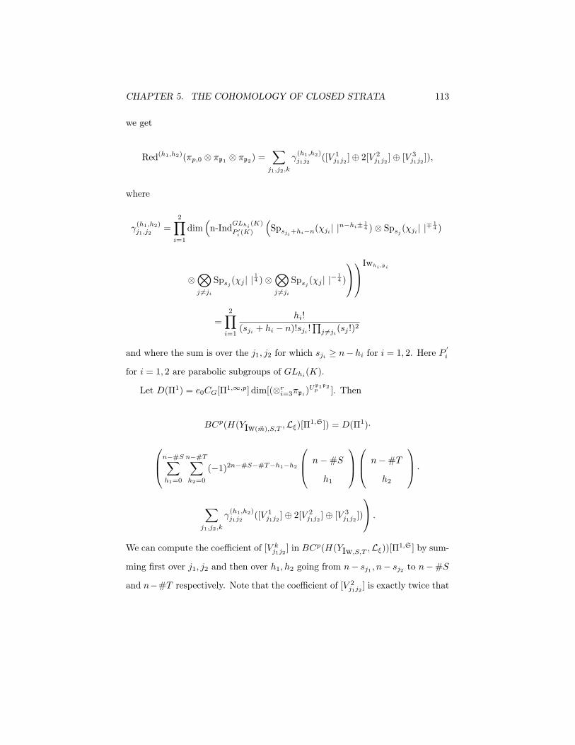
CHAPTER 5. THE COHOMOLOGY OF CLOSED STRATA 113
we get
Red(h1,h2)(πp,0 ⊗ πp1 ⊗ πp2) =∑
j1,j2,k
γ(h1,h2)j1j2
([V 1j1j2 ]⊕ 2[V 2
j1j2 ]⊕ [V 3j1j2 ]),
where
γ(h1,h2)j1,j2
=2∏
i=1
dim(n-IndGLhi
(K)
P ′i (K)
(Spsji+hi−n(χji | |n−hi± 1
4 )⊗ Spsj(χji | |∓
14 )
⊗⊗
j +=ji
Spsj(χj | |
14 )⊗
⊗
j +=ji
Spsj(χj | |−
14 )
Iwhi,pi
=2∏
i=1
hi!(sji + hi − n)!sji !
∏j +=ji
(sj !)2
and where the sum is over the j1, j2 for which sji ≥ n− hi for i = 1, 2. Here P′
i
for i = 1, 2 are parabolic subgroups of GLhi(K).
Let D(Π1) = e0CG[Π1,∞,p] dim[(⊗ri=3πpi)
Up1p2p ]. Then
BCp(H(YIw(%m),S,T ,Lξ)[Π1,S]) = D(Π1)·
n−#S∑
h1=0
n−#T∑
h2=0
(−1)2n−#S−#T−h1−h2
n−#S
h1
n−#T
h2
·
∑
j1,j2,k
γ(h1,h2)j1j2
([V 1j1j2 ]⊕ 2[V 2
j1j2 ]⊕ [V 3j1j2 ])
.
We can compute the coefficient of [V kj1j2 ] in BCp(H(YIw,S,T ,Lξ))[Π1,S] by sum-
ming first over j1, j2 and then over h1, h2 going from n− sj1 , n− sj2 to n−#S
and n−#T respectively. Note that the coefficient of [V 2j1j2 ] is exactly twice that

CHAPTER 5. THE COHOMOLOGY OF CLOSED STRATA 114
of [V 1j1j2 ] and of [V 3
j1j2 ]. The sum we get for [V 1j1j2 ] is
D(Π1)(n−#S)!(n−#T )!
(sj1 −#S)!(sj2 −#T )!sj1 !sj2 !∏
j +=j1(sj !)2
∏j +=j2
(sj !)2·
n−#S∑
h1=n−sj1
n−#T∑
h2=n−sj2
(−1)2n−#S−#T−h1−h2
sj1 −#S
h1 + sj1 − n
sj2 −#T
h2 + sj2−n
The sum in parentheses can be decomposed as
n−#S∑
h1=n−sj1
(−1)n−#S−h1
sj1 −#S
h1 + sj1 − n
·
n−#T∑
h2=n−sj2
(−1)n−#T−h2
sj2 −#T
h2 + sj2 − n
,
which is equal to 0 unless both sj1 = #S and sj2 = #T . So
BCp(H(YIw(%m),S,T ,Lξ)[Π1,S]) = D(Π1)·∑
sj1=#S,sj2=#T
(n−#S)!(n−#T )!sj1 !sj2 !∏j(sj !)4
·
([V 1
j1j2 ] + 2[V 2j1j2 ] + [V 3
j1j2 ]).
Since each YU,S,T is proper and smooth, it follows from the Weil conjec-
tures that Hj(YIw(%m),S,T ,Lξ) is strictly pure of weight mξ − 2tξ + j. This
property means that for some (hence every) lift σ of FrobF, every eigenvalue
of σ on Hj(YIw(%m),S,T ,Lξ) is a Weil qmξ−2tξ+j-number (see the definitions
above Lemma 1.4 of [TY]). However, the [V kj1j2 ] are strictly pure of weight
mξ−2tξ +2n−2− εk− (#S−1)− (#T −1) = mξ−2tξ +2n−#S−#T −2εk.
So
BCp(Hj(YIw(%m),S,T ,Lξ)[Π1,S]) = 0

CHAPTER 5. THE COHOMOLOGY OF CLOSED STRATA 115
unless j = 2n − #S − #T ± 1 or j = 2n − #S − #T . However, if the Igusa
cohomology is non-zero for some j = 2n−#S −#T ± 1, then there exist j1, j2
with sj1 = #S and sj2 = #T . Hence, the cohomology must also be non-zero
for j = 2n − #S − #T . The coefficients of [V kj1j2 ] all have the same sign, so
they are either strictly positive or strictly negative only depending on D(Π1).
However, BCp(H(YIw(m),S,T ,Lξ)[Π1,S] is an alternating sum, so the weight
2n−#S −#T ± 1 part of the cohomology should appear with a different sign
from the weight 2n−#S −#T part. This is a contradiction, so it must be the
case that πp1 * πp2 is tempered.
Corollary 5.3.4. Let n ∈ Z≥2 be an integer and L be any CM field. Let Π be
a cuspidal automorphic representation of GLn(AL) satisfying
• Π∨ * Π ◦ c
• Π∞ is cohomological for some irreducible algebraic representation Ξ.
Then Π is tempered at every finite place w of L.
Proof. By Lemma 1.4.3 of [TY], an irreducible smooth representation Π of
GLn(K) is tempered if and only if LK,n(Π) is pure of some weight. By Lemma
1.4.1 of [TY], purity is preserved under a restriction to the Weil-Deligne repre-
sentation of WK′ for a finite extension K ′/K of fields.
Fix a place v of L above p where p "= l. We will find a CM field F ′ such that
• F ′ = EF1, where E is an imaginary quadratic field in which p splits and
F1 = (F ′)c=1 has [F1 : Q] ≥ 2,
• F ′ is soluble and Galois over L,
• Π0F ′ = BCF ′/L(Π) is a cuspidal automorphic representation of GLn(AF ′),
and
• there is a place p of F above v such that Π0F ′,p has an Iwahori fixed vector,
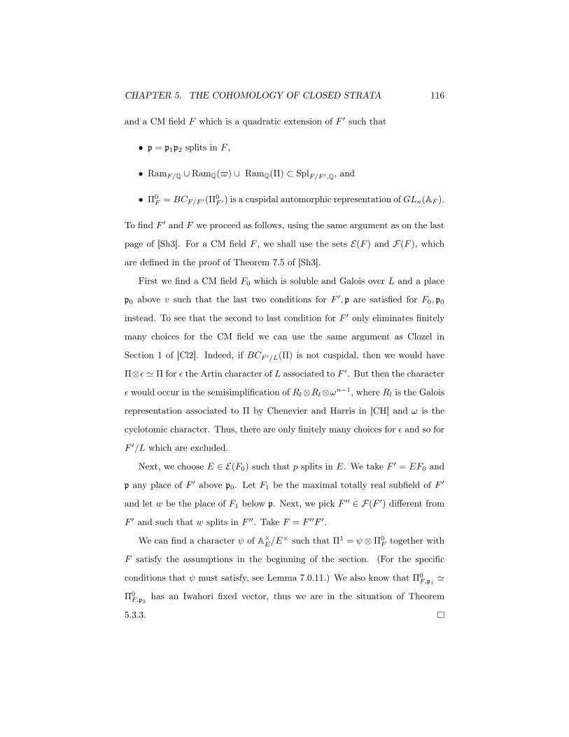
CHAPTER 5. THE COHOMOLOGY OF CLOSED STRATA 116
and a CM field F which is a quadratic extension of F ′ such that
• p = p1p2 splits in F ,
• RamF/Q ∪ RamQ(6) ∪ RamQ(Π) ⊂ SplF/F ′,Q, and
• Π0F = BCF/F ′(Π0
F ′) is a cuspidal automorphic representation of GLn(AF ).
To find F ′ and F we proceed as follows, using the same argument as on the last
page of [Sh3]. For a CM field F , we shall use the sets E(F ) and F(F ), which
are defined in the proof of Theorem 7.5 of [Sh3].
First we find a CM field F0 which is soluble and Galois over L and a place
p0 above v such that the last two conditions for F ′, p are satisfied for F0, p0
instead. To see that the second to last condition for F ′ only eliminates finitely
many choices for the CM field we can use the same argument as Clozel in
Section 1 of [Cl2]. Indeed, if BCF ′/L(Π) is not cuspidal, then we would have
Π⊗ε * Π for ε the Artin character of L associated to F ′. But then the character
ε would occur in the semisimplification of Rl⊗Rl⊗ωn−1, where Rl is the Galois
representation associated to Π by Chenevier and Harris in [CH] and ω is the
cyclotomic character. Thus, there are only finitely many choices for ε and so for
F ′/L which are excluded.
Next, we choose E ∈ E(F0) such that p splits in E. We take F ′ = EF0 and
p any place of F ′ above p0. Let F1 be the maximal totally real subfield of F ′
and let w be the place of F1 below p. Next, we pick F ′′ ∈ F(F ′) different from
F ′ and such that w splits in F ′′. Take F = F ′′F ′.
We can find a character ψ of A×E/E× such that Π1 = ψ ⊗Π0F together with
F satisfy the assumptions in the beginning of the section. (For the specific
conditions that ψ must satisfy, see Lemma 7.0.11.) We also know that Π0F,p1
*
Π0F,p2
has an Iwahori fixed vector, thus we are in the situation of Theorem
5.3.3.

CHAPTER 5. THE COHOMOLOGY OF CLOSED STRATA 117
Proposition 5.3.5. Assume again that the conditions in the beginning of this
section are satisfied and that Π0p1* Π0
p2has a nonzero Iwahori fixed vector.
Then
BCp(Hj(YIw(%m),S,T ,Lξ)[Π1,S]) = 0
unless j = 2n−#S −#T .
Proof. We will go through the same computation as in the proof of Theorem
5.3.3 except we will use the fact that πp1 * πp2 is tempered, so it is of the form
n-IndGLn(K)P (K) (Sps1
(χ1)× · · ·× Spst(χt)),
where the χj are unramified characters of K×.
We can compute Red(h1,h2)(πp,0 ⊗ πp1 ⊗ πp2) as in the proof of Theorem
5.3.3.
Ji
(n-IndGLn(K)
P (K) (Sps1(χ1)× · · ·× Spst
(χt) · |det |))
is equal to
∑[n-IndGLhi(k)
P ′i (K) (Spk1(χ1 ⊗ |det |s1−k1)× · · ·× Spkt
(χt ⊗ |det |st−kt))]
[n-IndGLhi(k)
P ′′i (K) (Sps1−k1(χ1)× · · ·× Spst−kt
(χt))],
where the sum is over all non-negative integers kj ≤ sj with hi =∑t
j=1 kj .
Let Vj1j2 = rec(χ−1
j1χ−1
j2| |1−n(ψu ◦NK/Eu
)−1). After we apply the functor
Groth(GLn−h1(K)×GLh1(K)×GLn−h2(K)×GLh2(K)×Q×p ) → Groth(FrobZF),
we get
Red(h1,h2)(πp,0 ⊗ πp1 ⊗ πp2) =∑
j1,j2,k
γ(h1,h2)j1j2
[Vj1j2 ]

CHAPTER 5. THE COHOMOLOGY OF CLOSED STRATA 118
where
γ(h1,h2)j1,j2
=2∏
i=1
dim
n-IndGLhi(K)
P ′i (K)
Spsji(χji | |n−hi)⊗
⊗
j +=ji
Spsj(χj)
Iwhi,pi
=2∏
i=1
hi!(sji + hi − n)!sji !
∏j +=ji
(sj !)2
and where the sum is over the j1, j2 for which sji ≥ n− hi for i = 1, 2. Here P′
i
for i = 1, 2 are parabolic subgroups of GLhi(K).
Let D(Π1) = e0CG[Π1,∞,p] dim[(⊗ri=3πpi)
Up1p2p ]. The same computation as
in the proof of Theorem 5.3.3 gives us
BCp(H(YIw(%m),S,T ,Lξ)[Π1,S])
= D(Π1) ·∑
sj1=#S,sj2=#T
(n−#S)!(n−#T )!sj1 !sj2 !∏j(sj !)2
[Vj1j2 ].
Since πp1 * πp2 is tempered, we know that [Vj1j2 ] is strictly pure of weight 2n−
#S−#T . The Weil conjectures tell us then that BCp(Hj(YIw(%m),S,T ,Lξ)[Π1,S]) =
0 unless j = 2n−#S −#T .

Chapter 6
The cohomology of Igusa
varieties
The goal of this chapter is to explain how to prove Theorem 5.3.1. The proof
will be a straightforward generalization of the proof of Theorem 6.1 of [Sh3] and
so we will follow closely the argument and the notation of that paper.
We will summarize without proof the results in [Sh3] on transfer and on the
twisted trace formula. We will emphasize the place ∞, since that is the only
place of Q where our group G differs from the group G considered in [Sh3]. All
of the results and notation are as in [Sh3], except in the proof of Lemmas 6.0.8
and 6.0.9, where we also use the notation of [Sh2].
We start by explaining the notation we will be using throughout this section,
which is consistent with the notation of [Sh3]. Recall that we have fixed a unitary
similitude group G over Q, which satisfies certain local conditions as in Lemma
2.1.1. In this section, will work with a quasi-split form of G, denoted by Gn as
well as with groups Gn1,n2 which are endoscopic groups for Gn. We will denote
an element in the set {Gn} ∪ {Gn1,n2 |n1 + n2 = n, n1 ≥ n2 > 0)} as G%n, where
119

CHAPTER 6. THE COHOMOLOGY OF IGUSA VARIETIES 120
-n is a multiset of positive integers (in our case, -n will have length 1 or 2). In
other words, -n runs through the elements of the set {n} ∪ {(n1, n2)|n1 + n2 =
n, n1 ≥ n2 > 0}.
If r ∈ {1, 2} and -n = (ni)ri=1 with ni ∈ Z>0 define
GL%n :=r∏
i=1
GLni .
Let i%n : GL%n ↪→ GLN (N =∑
i ni) be the natural map. Let
Φ%n = i%n(Φn1 , . . . , ,Φnj ),
where Φn is the matrix in GLn with entries (Φn)ij = (−1)i+1δi,n+1−j .
Let K be some local non-archimedean local field and H a connected reductive
group over K. We will denote by Irr(H(K)) (resp. Irrl(H(K))) the set of
isomorphism classes of irreducible admissible representations of G(K) over C
(resp. over Ql). Let C∞c (H(K)) be the space of smooth compactly supported
C-valued functions on H(K). Let P be a K-rational parabolic subgroup of H
with a Levi subgroup M . For πM ∈ Irr(M(K)) and π ∈ Irr(H(K)) we can define
the normalized Jacquet module JHP (π) and the normalized parabolic induction
n-IndHP πM . We can define a character δP : M(K) → R×>0 by
δP (m) = |det(ad(m))|Lie(P )/Lie(M)|K .
We can view δP as a character valued in Q×l via ι−1l .
If
J (h)(Qp) * D×K, 1
n−h×GLh(K),
where K/Qp is finite, then we define δ12P (J(h))
(g) := δ12Pn−h,h
(g∗),where g∗ ∈
GLn−h(K)×GLh(K) is any element whose conjugacy class matches that of g.

CHAPTER 6. THE COHOMOLOGY OF IGUSA VARIETIES 121
If
J (h1,h2) * GL1 ×2∏
i=1
(D×Fpi , 1
n−hi
×RFpi/QpGLhi)×
∏
i>2
RFpi/QpGLn,
we define δ12P (J(h1,h2 )
: J (h1,h2)(Qp) → Q×l to be the product of the characters
δ12P (J(hi))
for i = 1, 2.
Let -n = (ni)ri=1 for some r ∈ {1, 2} and ni ∈ Z>0. Let G%n be the Q-group
defined by
G%n(R) = {(λ, gi) ∈ GL1(R)×GL%n(F ⊗Q R) | gi · Φ%n ·t gci = λΦ%n}
for any Q-algebra R. For any -n, the group G%n is quasi-split over Q. In particular,
our unitary group G is an inner form of Gn. Since G is quasi-split at all finite
places, there exists an isomorphism
G×Q A∞ * Gn ×Q A∞;
we fix such an isomorphism.
Also define
G%n = RE/Q(G%n ×Q E).
Let θ denote the action on G%n induced by (id, c) on G%n×Q E. Let ε : Z → {0, 1}
be the unique map such that ε(n) ≡ n (mod 2). Let 6 : A×E/E× → C× be any
Hecke character such that 6|A×/Q× is the composite of ArtQ and the natural
surjective character WQ ! Gal(E/Q) ∼→ {±1}. Using the Artin map ArtE , we
view 6 as a character WE → C× as well.
Assume that RamF/Q ∪ RamQ(6) ⊂ SplF/F2,Q.
Let Eell(Gn) be a set of representatives of isomorphism classes of elliptic
endoscopic triples for Gn over Q. Then Eell(Gn) can be identified with the set

CHAPTER 6. THE COHOMOLOGY OF IGUSA VARIETIES 122
of triples
{(Gn, sn, ηn} ∪{Gn1,n2 , sn1,n2 , ηn1,n2 | n1 + n2 = 0, n1 ≥ n2 > 0},
where (n1, n2) may be excluded in some cases. As we are only interested in the
stable part of the cohomology of Igusa varieties, we will not be concerned with
these exclusions so we will ignore them in this paper. Here sn = 1 ∈ Gn, sn1,n2 =
(1, (In1 ,−In2)) ∈ Gn1,n2 , ηn : Gn → Gn is the identity map whereas
ηn1,n2 : (λ, (g1, g2)) 2→
λ,
g1 0
0 g2
.
We can extend ηn1,n2 to a morphism of L-groups, which sends z ∈ WE to
6(z)−N(n1,n2),
6(z)ε(n−n1) · In1 0
0 6(z)ε(n−n2) · In2
! z.
Similarly we can also define a morphism of L-groups
ζn1,n2 :L Gn1,n2 →L Gn,
which extends the map
ζn1,n2 : Gn1,n2 → Gn
(λ+, λ−, (gσ,1, gσ,2)) 2→
λ+, λ−
gσ,1 0
0 gσ,2
(See section 3.2 of [Sh3] for the precise definition.) We have the following com-

CHAPTER 6. THE COHOMOLOGY OF IGUSA VARIETIES 123
mutative diagram of L-morphisms.
LGn1,n2
BCn1,n2
""
ηn1,n2 !! LGn
BCn
""LGn1,n2
ζn1,n2
!! LGn
We will proceed to define local transfers for each of the arrows in the above
commutative diagram so that these transfers are compatible.
Choose the normalization of the local transfer factor ∆v( , )GnG$n
defined in
Section 3.4 of [Sh3]. It is possible to give a concrete description of the ∆v( , )GnG$n
-
transfer at finite places v of Q between functions in C∞c (Gn(Qv)) and functions
in C∞c (Gn1,n2(Qv)) as long as v satisfies at least one of the conditions:
• v ∈ UnrF/Q and v "∈ RamQ(6),
• v ∈ SplE/Q,
• v ∈ SplF/F2,Q and v "∈ SplE/Q.
The transfer φn1,n2v of φn
v ∈ C∞c (Gn(Qv)) and φnv will satisfy an identity involv-
ing orbital integrals. Since we are assuming that RamF/Q ⊆ SplF/F2,Q, we can
define the transfer at all places v of Q.
It is also possible to define a transfer of pseudo-coefficients at infinity. Con-
sider (G%n, s%n, η%n) ∈ Eell(Gn), which is also an endoscopic triple for G. Fix real
elliptic maximal tori T ⊂ G and TG$n⊂ G%n together with an R-isomorphism
j : TG$n
∼→ T. Also fix a Borel subgroup B of G over C containing TC. Shelstad
defined the transfer factor ∆j,B , see [She].
Let ξ be an irreducible algebraic representation of GC. Define χξ : AG,∞ → C
to be the restriction of ξ to AG,∞ (the connected component of the identity in the
R-points of the maximal Q-split torus in the center of G). Choose K∞ ⊂ G(R)

CHAPTER 6. THE COHOMOLOGY OF IGUSA VARIETIES 124
to be a maximal compact subgroup (admissible in the sense of [Art]) and define
q(G) =12
dim(G(R)/K∞AG,∞) = 2n− 2.
For each π ∈ Πdisc(G(R), ξ∨) there exists φπ ∈ C∞c (G(R), χξ) a pseudo-
coefficient for π. Any discrete L-parameter ϕG$nsuch that η%nϕG$n
∼ ϕξ corre-
sponds to an L-packet of the form Πdisc(G%n(R), ξ(ϕG$n)∨). Define
φG$n,ξ(ϕG$n) :=
1|Π(ϕ%n)|
∑
πG$n
φπG$nand
φG$nπ := (−1)q(G)
∑
ηϕG$n∼ϕξ
〈aω∗(ϕG$n,ξ)ωπ, s〉det(ω∗(ϕG$n,ξ)) · φG$n,ξ(ϕG$n) .
Then φG$nπ is a ∆j,B-transfer of φπ.
We will now review the base change for the groups G%n and G%n. Define the
group
G+%n := (RE/QGL1 ×RF/QGL%n) ! {1, θ},
where θ(λ, g)θ−1 = (λc, λcg#) and g# = Φ%ntgcΦ−1
%n . If we denote by G0%n and
G0%nθ the cosets of {1} and {θ} in G+
%n then G+%n = G0
%n
∐G0
%nθ. There is a natural
Q-isomorphism G%n∼→ G0
%n which extends to
G%n ! Gal(E/Q) ∼→ G+%n
so that c ∈ Gal(E/Q) maps to θ.
Let v be a place of Q. A representation Πv ∈ Irr(G%n(Qv)) is called θ-stable if
Πv * Πv ◦θ as representations of G%n(Qv). If that is the case, then we can choose
an operator AΠv on the representation space of Πv which induces Πv∼→ Πv ◦ θ
and which satisfies A2Πv
= id. Such an operator is called normalized and it
is pinned down up to sign. We can similarly define the notion of θ-stable for

CHAPTER 6. THE COHOMOLOGY OF IGUSA VARIETIES 125
ΠS ∈ Irr(G%n(AS)) and a corresponding intertwining operator AΠS for any finite
set S of places of Q. There is a correspondence between θ-stable representations
of G%n(Qv) together with a normalized intertwining operator and representations
of G+%n (Qv). We also mention that in order for a representation Π ∈ Irr(G%n(A))
to be θ-stable it is necessary and sufficient that Π = ψ ⊗Π1 satisfy
• (Π1)∨ * Π1 ◦ c, and
•∏r
i=1 ψi = ψc/ψ where ψΠ1 = ψ1⊗ · · ·⊗ψr is the central character of Π1.
Now we shall discuss BC-matching functions. It is possible to construct for each
finite place v of Q and fv ∈ C∞c (G%n(Qv)) a function φv ∈ C∞c (G%n(Qv)), which
is the BC-transfer of fv. The transfer can be described concretely in the cases
v ∈ UnrF/Q and v ∈ SplF/F2,Q, except that in the case v ∈ UnrF/Q we have the
condition that fv must be unramified. Moreover, we also have an explicit map
BC%n : Irr(ur)(G%n(Qv)) → Irr(ur)θ-st(G%n(Qv))
where the representations must be unramified in the case v ∈ UnrF/Q and where
there is no restriction in the case v ∈ SplF/F2,Q. There are normalized operators
A0Πv
: Πv∼→ Πv ◦ θ such that if Πv = BC%n(πv) and φv and fv are BC-matching
functions then
tr(Πv(fv)A0Πv
) = trπv(φv).
Note that left side of the above equality computes the trace of fvθ, the function
on G%nθ obtained from fv via translation by θ.
The next step is to consider the base change at ∞. Let ξ%n be an irreducible
algebraic representation of G%n,C . Consider the natural isomorphism
G%n(C) * G%n(C)×G%n(C).

CHAPTER 6. THE COHOMOLOGY OF IGUSA VARIETIES 126
We can define a representation Ξ%n of G%n by Ξ%n := ξ%n⊗ξ%n. It is possible to find an
irreducible, θ-stable, generic unitary representation ΠΞ$n∈ Irr(G%n(R), χ−1
ξ$n) to-
gether with a normalized operator A0ΠΞ$n
and a function fG$n,Ξ$n∈ C∞c (G(R), χξ$n
)
such that
• ΠΞ$nis the base change of the L-packet Πdisc(G%n(R), ξ∨%n ),
• tr(ΠΞ$n(fG$n,Ξ$n
) ◦A0ΠΞ$n
) = 2 and
• fG$n,Ξ$nand φG$n,ξ$n
are BC-matching functions (where φG$n,ξ$nis defined as
a pseudocoefficient for the L-packet Πdisc(G%n(R), ξ∨%n ).
The transfer for ζn1,n2 can be defined explicitly since the groups G%n are es-
sentially products of general linear groups. It can be checked that for all finite
places v of Q the transfers are compatible. For v = ∞ we have the compatibility
relation on the representation-theoretic side follows directly from the commu-
tative diagram of L-morphisms.
Now we shall describe the transfer factors ∆v( , )GG$n
. At v "= ∞ we can
choose
∆v( , )GG$n
= ∆0v( , )Gn
G$n,
via the fixed isomorphism G ×Q A∞ * Gn ×Q A∞. We choose the unique
∆∞( , )GG$n
such that the product formula
∏
v
∆v(γG$n, γ)G
G$n= 1
holds for any γ ∈ G(Q) semisimple and γG$n∈ G%n(A) a (G, G%n)-regular semisim-
ple element such that γ and γG$nhave matching stable conjugacy classes. Let
e%n(∆∞) ∈ C× denote the constant for which
∆∞(γG$n, γ)G
G$n= e%n(∆∞)∆j,B(γG$n
, γ)

CHAPTER 6. THE COHOMOLOGY OF IGUSA VARIETIES 127
holds. Note that for -n = (n), e%n(∆∞) = 1.
Let φ∞,p ·φ′p ∈ C∞c (G(A∞,p)×J (h1,h2)(Qp)) be a complex-valued acceptable
function. (For a definition of the notion of acceptable function, see Definition 6.2
of [Sh1]). For each G%n ∈ Eell(G) we define the function φ%nIg on G%n(A) (assuming
that φ∞,p =∏
v +=p,∞ φv). For v "= p,∞, we take φ%nIg,v ∈ C∞c (G%n(Qv)) to be the
∆v( , )GG$n
-transfer of φv. We take
φ%nIg,∞ := e%n(∆∞) · (−1)q(G)〈µh, s%n〉
∑
ϕ$n
det(ω∗(ϕG$n)) · φG$n,ξ(ϕ$n),
where ϕ%n runs over L-parameters such that η%nϕ%n ∼ ϕξ and ξ(ϕ%n) is the
algebraic representation of G%n,C such that the L-packet associated to ϕ%n is
Πdisc(G%n(R), ξ(ϕ%n)∨).
We also take
φ%nIg,p ∈ C∞c (G%n(Qp))
to be the function constructed from φ′p in section 6.3 of [Sh2]. We shall summa-
rize the construction of φ%nIg,p in the case -n = (n). By definition (see the formula
above Lemma 6.5 of [Sh2])
φ%nIg,p =
∑
(MGn,sGn,ηGn)
cMGn· φMGn
p ,
where the sum is taken over G-endoscopic triples for J (h1,h2). The set I(MGn , Gn)
(which can be identified with a set of cosets of Out(MGn , sGn , ηGn)) consists of
only one element in our case, so we suppress the index i ∈ I(MGn , Gn) in
φMGn ,ip . Each φ
MGnp ∈ C∞c (Gn(Qp)) is constructed from a function φ
MGnp ∈
C∞c (MGn(Qp)) which is a ∆p( , )J(h1,h2)
MGn-transfer of a normalized φ′p.
The following proposition is Theorem 7.2 of [Sh2].
Proposition 6.0.6. If φ∞,p · φ′p ∈ C∞c (G(A∞,p) × J (h1,h2)(Qp)) is acceptable,

CHAPTER 6. THE COHOMOLOGY OF IGUSA VARIETIES 128
then
tr(φ∞,p ·φ′p|ιlHc(Ig(h1,h2),Lξ)) = (−1)h1+h2 | ker1(Q, G)|∑
G$n
ι(G, G%n)STG$ne (φ%n
Ig)
where the sum runs over the set Eell(G) of elliptic endoscopic triples (G%n, s%n, η%n).
Remark 6.0.7. Theorem 7.2 of [Sh2] is proved under the “unramified hypothesis”,
however, the only place where this hypothesis is needed is in the proof of Lemma
11.1 of [Sh1]. Lemma 5.2.1 provides an alternative to the proof of Lemma 11.1
of [Sh1] in our situation, so the results of [Sh1] and [Sh2] carry over. For details,
see the discussion in the beginning of Section 5.2 of [Sh3]. The sign (−1)h1+h2
does not show up in the statement of the theorem in [Sh2], but we need to
include it because our convention for the alternating sum of the cohomology
differs from the usual one by (−1)h1+h2 .
The constants ι(G, G%n) = τ(G)τ(G%n)−1|Out(G%n, s%n, η%n)|−1 can be com-
puted explicitly. We mention that
|Out(G%n, s%n, η%n)| =
2 if -n = (n2 , n
2 )
1 otherwise.
We also have by Corollary 4.7 of [Sh3] the relation
IG$nθgeom(fθ) = τ(G%n)−1 · STG$n
e (φ),
when φ and f are BC-matching functions, i.e.
φ = φS · φSfin · φG$n,ξ and f = fS · fSfinfG$n,Ξ,
with φS a BC-transfer of fS and φSfin a BC-transfer of fSfin .Thus, assuming

CHAPTER 6. THE COHOMOLOGY OF IGUSA VARIETIES 129
that for each -n there exists f%n such that φ%nIg and f%n are BC-matching, we can
write
tr(φ∞,p · φ′p|ιlHc(Ig(h1,h2),Lξ)) = | ker1(Q, G)| · τ(G)∑
G$n
ε%nIG$nθgeom(f%nθ),
where ε%n = 12 if -n = (n
2 , n2 ) or 1 otherwise.
Furthermore, the twisted trace formula by Arthur, is an equality between
IG$nθspec(fθ) = IG$nθ
geom(fθ).
By combining Proposition 4.8 and Corollary 4.14 of [Sh3] we can compute
IG$nθspec(fθ) as
∑
M
|WM ||WG$n
| |det(Φ−1%n θ − 1)
aG$nθ
M
|−1∑
ΠM
tr(n-IndG$nQ (ΠM )ξ(f) ◦A′n-IndG$n
Q (ΠM )ξ,
where M runs over Q-Levi subgroups of G%n containing a fixed minimal Levi and
Q is a parabolic containing M as a Levi. The rest of the notation is defined on
pages 31 and 32 of [Sh3]. Note that A′n-IndG$nQ (ΠM )ξ
is a normalized intertwining
operator for n-IndG$nQ (ΠM )ξ.
We will be particularly interested in making the above formula explicit when
-n = (n). In that case, IG$nθspec(fθ) is a sum of
12
∑
Π′
tr(Π′ξ(f)A′Π′ξ),
where Π′ runs over θ-stable subrepresentations of RGn,disc, and
∑
M"Gn
|WM ||WGn|
|det(Φ−1n θ − 1)aGnθ
M|−1
∑
Π′M
tr(n-IndGnQ (Π′M )ξ(f) ◦A′n-IndGn
Q (Π′M )ξ),
where Π′M runs over Φ−1n θ-stable subrepresentations of RM,disc.
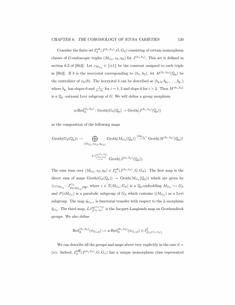
CHAPTER 6. THE COHOMOLOGY OF IGUSA VARIETIES 130
Consider the finite set Eeffp (J (h1,h2), G,G%n) consisting of certain isomorphism
classes of G-endoscopic triples (MG$n, s%n, η%n) for J (h1,h2). This set is defined in
section 6.2 of [Sh2]. Let cMG$n∈ {±1} be the constant assigned to each triple
in [Sh2]. If b is the isocrystal corresponding to (h1, h2), let M (h1,h2)(Qp) be
the centralizer of νG(b). The isocrystal b can be described as (bp,0, bp1 , . . . , bpr )
where bpi has slopes 0 and 1n−hi
for i = 1, 2 and slope 0 for i > 2. Then M (h1,h2)
is a Qp -rational Levi subgroup of G. We will define a group morphism
n-Red(h1,h2)%n : Groth(G%n(Qp) → Groth(J (h1,h2)(Qp))
as the composition of the following maps
Groth(G%n(Qp)) →⊕
(MG$n,sG$n
,ηG$n)
Groth(MG$n(Qp))
⊕ηG$n,∗−→ Groth(M (h1,h2)(Qp))
LJM(h1,h2)
J(h1,h2)−→ Groth(J (h1,h2)(Qp)).
The sum runs over (MG$n, s%n, η%n) ∈ Eeff
p (J (h1,h2), G,G%n). The first map is the
direct sum of maps Groth(G%n(Qp)) → Groth(MG$n(Qp)) which are given by
⊕icMG$n· JG$n
P (iMG$n)op, where i ∈ I(MG$n
, G%n) is a Qp-embedding MG$n↪→ G%n
and P (iMG$n) is a parabolic subgroup of G%n which contains i(MG$n
) as a Levi
subgroup. The map ηG$n,∗ is functorial transfer with respect to the L-morphism
ηG$n. The third map, LJM(h1,h2)
J(h1,h2) is the Jacquet-Langlands map on Grothendieck
groups. We also define
Red(h1,h2)%n (πG$n,p) := n-Red(h1,h2)
%n (πG$n,p)⊗ δ12P (J(h1,h2))
We can describe all the groups and maps above very explicitly in the case -n =
(n). Indeed, Eeffp (J (h1,h2), G,Gn) has a unique isomorphism class represented

CHAPTER 6. THE COHOMOLOGY OF IGUSA VARIETIES 131
by
(MGn , sGn , ηGn) = (M (h1,h2), 1, id).
The set I(MGn , Gn) is also a singleton in this case, so we suppress i everywhere.
This means that we can also take ηGn = id and ηGn,∗ = id and by Remark 6.4
of [Sh2], we may also take cMGn= ep(J (h1,h2)), which is the Kottwitz sign of
the Qp-group J (h1,h2). There are isomorphisms
G(Qp) * Q×p ×GLn(Fp1)×GLn(Fp2)×∏
i>2
GLn(Fpi),
M (h1,h2)(Qp) * Q×p ×(GLn−h1(Fp1)×GLh1(Fp1))×(GLn−h2(Fp2)×GLh2(Fp2))
×∏
i>2
GLn(Fpi),
J (h1,h2)(Qp) * Q×p ×(D×Fp1 , 1
n−h1×GLh1(Fp1))×(D×
Fp2 , 1n−h2
×GLh2(Fp2))×∏
i>2
GLn(Fpi).
Thus, ep(J (h1,h2)) = (−1)2n−2−h1−h2 . If we write πp = πp,0 ⊗ (⊗iπpi), then we
have
Red(h1,h2)n (πp) = (−1)h1+h2πp,0⊗Redn−h1,h1(πp1)⊗Redn−h2,h2(πp2)⊗(⊗i>2πpi).
Lemma 6.0.8. For any πp ∈ Groth(Gn(Qp))
trπp(φnIg,p) = tr(Red(h1,h2)
n (πp))(φ′p).
Proof. Set M = MGn . We know that φnIg,p = ep(J (h1,h2)) · φM
p . By Lemma 3.9
of [Sh2],
trπp(φMp ) = tr(JGn
P opM
(πp))(φMp ).
Here φMp is a ∆p( , )J(h1,h2)
M ≡ ep(J (h1,h2))-transfer of φ0p = φ′p · δ
12P (J(h1,h2))
(by
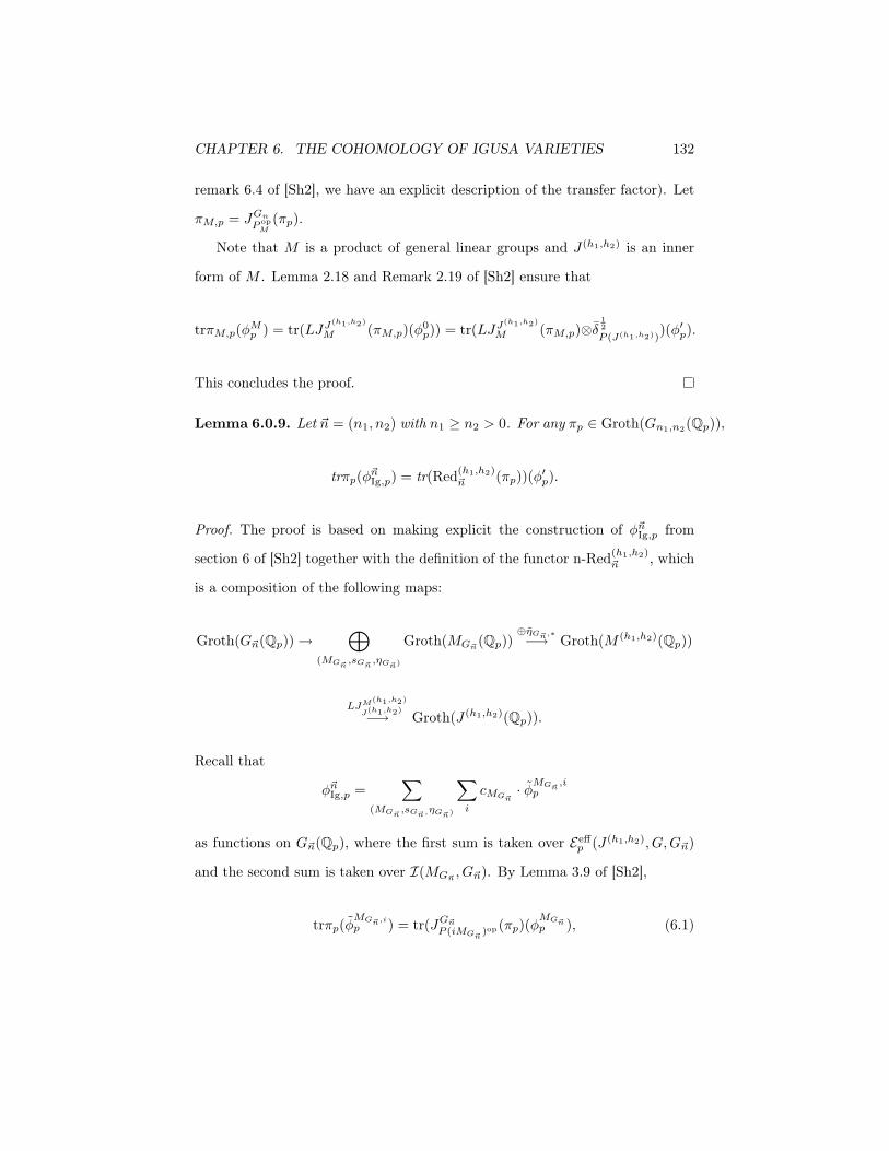
CHAPTER 6. THE COHOMOLOGY OF IGUSA VARIETIES 132
remark 6.4 of [Sh2], we have an explicit description of the transfer factor). Let
πM,p = JGn
P opM
(πp).
Note that M is a product of general linear groups and J (h1,h2) is an inner
form of M . Lemma 2.18 and Remark 2.19 of [Sh2] ensure that
trπM,p(φMp ) = tr(LJJ(h1,h2)
M (πM,p)(φ0p)) = tr(LJJ(h1,h2)
M (πM,p)⊗δ12P (J(h1,h2))
)(φ′p).
This concludes the proof.
Lemma 6.0.9. Let -n = (n1, n2) with n1 ≥ n2 > 0. For any πp ∈ Groth(Gn1,n2(Qp)),
trπp(φ%nIg,p) = tr(Red(h1,h2)
%n (πp))(φ′p).
Proof. The proof is based on making explicit the construction of φ%nIg,p from
section 6 of [Sh2] together with the definition of the functor n-Red(h1,h2)%n , which
is a composition of the following maps:
Groth(G%n(Qp)) →⊕
(MG$n,sG$n
,ηG$n)
Groth(MG$n(Qp))
⊕ηG$n,∗−→ Groth(M (h1,h2)(Qp))
LJM(h1,h2)
J(h1,h2)−→ Groth(J (h1,h2)(Qp)).
Recall that
φ%nIg,p =
∑
(MG$n,sG$n,ηG$n)
∑
i
cMG$n· φMG$n
,ip
as functions on G%n(Qp), where the first sum is taken over Eeffp (J (h1,h2), G,G%n)
and the second sum is taken over I(MG$n, G%n). By Lemma 3.9 of [Sh2],
trπp(φMG$n,ip ) = tr(JG$n
P (iMG$n)op(πp)(φ
MG$np ), (6.1)

CHAPTER 6. THE COHOMOLOGY OF IGUSA VARIETIES 133
where φMG$np ∈ C∞c (MG$n
(Qp)) is a ∆p( , )J(h1,h2)
MG$n-transfer of φ0
p = φ′p·δ12P (J(h1,h2))
.
Equation 6.1 tells us that
trπp(φ%nIg,p) =
∑
(MG$n,sG$n,ηG$n)
tr(fMG$n(πp))(φ
MG$np ), (6.2)
where fMG$n(πp) = ⊕icMG$n
JG$n
P (iMG$n)(πp). The first map in the definition of
Red(h1,h2)%n is the direct sum of fMG$n
over all (MG$n, s%n, η%n).
The function φMG$np is a ∆p( , )M(h1,h2)
MG$n-transfer of the function φ∗p ∈
C∞c (M (h1,h2)(Qp)) which is itself a transfer of φ0p via ∆p( , )J(h1,h2)
M(h1,h2) ≡ ep(J (h1,h2)).
(All transfer factors are normalized as in [Sh2].) We will focus on making the
∆p( , )M(h1,h2)
MG$n-transfer explicit first, for which we need to have a complete
description of all endoscopic triples (MG$n, sG$n
, ηG$n).
We have the following isomorphisms over Qp.
G * GL1 ×∏
i≥1
RFpi/QpGLn
Gn1,n2 * GL1 ×∏
i≥1
RFpi/QpGLn1,n2
M (h1,h2) * GL1 ×2∏
i=1
RFpi/QpGLn−hi,hi ×
∏
i>2
RFpi/QpGLn
J (h1,h2) * GL1 ×2∏
i=1
(D×Fpi , 1
n−hi
×GLhi)×∏
i>2
RFpi/QpGLn.
Consider also the following four groups over Qp, which can be thought of as
Levi subgroups of Gn1,n2 via the block diagonal embeddings.
MG$n,1 := GL1 ×2∏
i=1
RFpi/Qp
GLn−hi,hi−n2,n2 ×∏
i>2
RFpi/QpGLn1,n2

CHAPTER 6. THE COHOMOLOGY OF IGUSA VARIETIES 134
MG$n,2 := GL1 ×2∏
i=1
RFpi/Qp
GLn−hi,hi−n1,n1 ×∏
i>2
RFpi/QpGLn1,n2
MG$n,3 := GL1 ×2∏
i=1
RFpi/Qp
GLn−hi,hi−ni,ni ×∏
i>2
RFpi/QpGLn1,n2
MG$n,4 := GL1 ×2∏
i=1
RFpi/Qp
GLn−hi,hi−n3−i,n3−i ×∏
i>2
RFpi/QpGLn1,n2
Note that we only define MG$n,j when it makes sense, for example MG$n,1 is
defined only when hi ≥ n2 for i = 1, 2. We define ηG$n,j : MG$n,j → M (h1,h2) to
be the obvious block diagonal embedding. We also let
sMG$n,j = (1, (±1,±1,±1)i=1,2, (1, 1)i>2),
where the signs on the Fpi-component are chosen such that sMG$n,j is positive
on the GLn1-block of the Fpi-component and negative on the GLn2-block of the
Fpi-component.
It is easy to check, as on page 42 of [Sh3], that Eeffp (J (h1,h2), G,G%n) consists
of those triples (MG$n,j , sG$n,j , ηG$n,j) which make sense. For example, if hi < n2
for i = 1, 2 then Eeff(J (h1,h2), G,G%n) is empty, but if hi ≥ n1 for i = 1, 2 then
Eeff(J (h1,h2), G,G%n) consists of four elements. The key point is to notice that
for a triple (MG$n, sG$n
, ηG$n) to lie in Eeff(J (h1,h2), G,G%n) it is necessary for sG$n
to transfer to an element of the dual group M (h1,h2) = J (h1,h2) which is either
+1 or −1 in the GLn−hi(C) block of the Fpi-component.
We can extend ηG$n,j to an L-morphism ηG$n,j : LMG$n,j → LM (h1,h2) which is
compatible with the L-morphism η%n : LG%n →L G, when we map LMG$n,jlj→ LG%n
and LM (h1,h2) l→ LG via (a conjugate of) the obvious block diagonal embedding
(where we always send the GLn1-block to the top left corner and the GLn2-block
to the bottom right corner). The morphism ηG$n,j is defined as on page 42 of
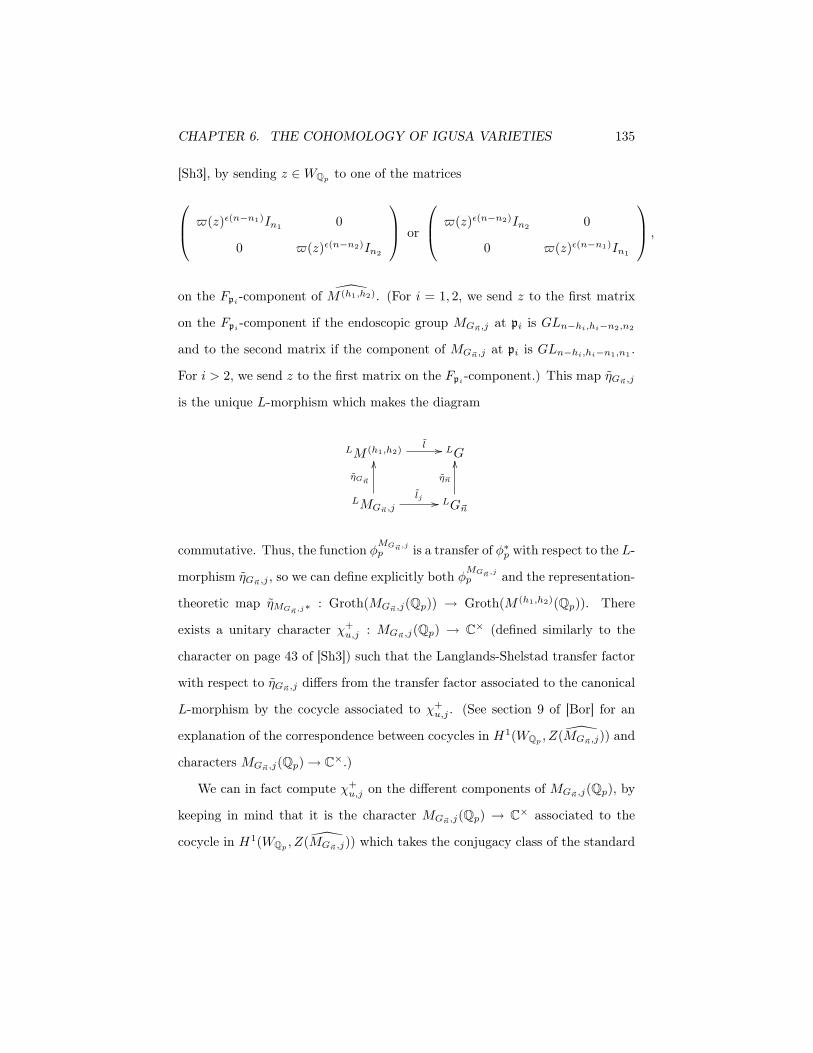
CHAPTER 6. THE COHOMOLOGY OF IGUSA VARIETIES 135
[Sh3], by sending z ∈ WQp to one of the matrices
6(z)ε(n−n1)In1 0
0 6(z)ε(n−n2)In2
or
6(z)ε(n−n2)In2 0
0 6(z)ε(n−n1)In1
,
on the Fpi-component of M (h1,h2). (For i = 1, 2, we send z to the first matrix
on the Fpi-component if the endoscopic group MG$n,j at pi is GLn−hi,hi−n2,n2
and to the second matrix if the component of MG$n,j at pi is GLn−hi,hi−n1,n1 .
For i > 2, we send z to the first matrix on the Fpi-component.) This map ηG$n,j
is the unique L-morphism which makes the diagram
LM (h1,h2)l !! LG
LMG$n,jlj !!
ηG$n
##
LG%n
η$n
##
commutative. Thus, the function φMG$n,jp is a transfer of φ∗p with respect to the L-
morphism ηG$n,j , so we can define explicitly both φMG$n,jp and the representation-
theoretic map ηMG$n,j∗ : Groth(MG$n,j(Qp)) → Groth(M (h1,h2)(Qp)). There
exists a unitary character χ+u,j : MG$n,j(Qp) → C× (defined similarly to the
character on page 43 of [Sh3]) such that the Langlands-Shelstad transfer factor
with respect to ηG$n,j differs from the transfer factor associated to the canonical
L-morphism by the cocycle associated to χ+u,j . (See section 9 of [Bor] for an
explanation of the correspondence between cocycles in H1(WQp , Z(MG$n,j)) and
characters MG$n,j(Qp) → C×.)
We can in fact compute χ+u,j on the different components of MG$n,j(Qp), by
keeping in mind that it is the character MG$n,j(Qp) → C× associated to the
cocycle in H1(WQp , Z(MG$n,j)) which takes the conjugacy class of the standard
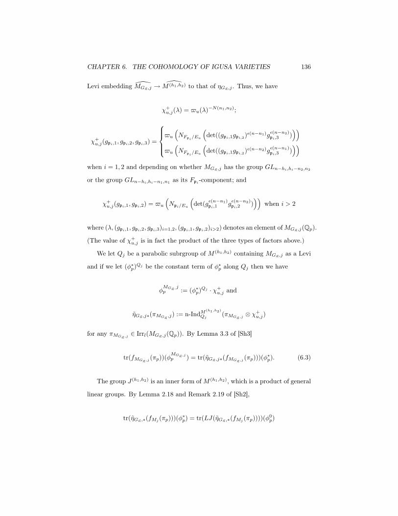
CHAPTER 6. THE COHOMOLOGY OF IGUSA VARIETIES 136
Levi embedding MG$n,j → M (h1,h2) to that of ηG$n,j . Thus, we have
χ+u,j(λ) = 6u(λ)−N(n1,n2);
χ+u,j(gpi,1, gpi,2, gpi,3) =
6u
(NFpi/Eu
(det((gpi,1gpi,2)ε(n−n1)gε(n−n2)
pi,3 )))
6u
(NFpi/Eu
(det((gpi,1gpi,2)ε(n−n2)gε(n−n1)
pi,3 )))
when i = 1, 2 and depending on whether MG$n,j has the group GLn−hi,hi−n2,n2
or the group GLn−hi,hi−n1,n1 as its Fpi-component; and
χ+u,j(gpi,1, gpi,2) = 6u
(Npi/Eu
(det(gε(n−n1)
pi,1 gε(n−n2)pi,2 )
))when i > 2
where (λ, (gpi,1, gpi,2, gpi,3)i=1,2, (gpi,1, gpi,2)i>2) denotes an element of MG$n,j(Qp).
(The value of χ+u,j is in fact the product of the three types of factors above.)
We let Qj be a parabolic subrgroup of M (h1,h2) containing MG$n,j as a Levi
and if we let (φ∗p)Qj be the constant term of φ∗p along Qj then we have
φMG$n,jp := (φ∗p)
Qj · χ+u,j and
ηG$n,j∗(πMG$n,j) := n-IndM(h1,h2)
Qj(πMG$n,j ⊗ χ+
u,j)
for any πMG$n,j ∈ Irrl(MG$n,j(Qp)). By Lemma 3.3 of [Sh3]
tr(fMG$n,j (πp))(φMG$n,jp ) = tr(ηG$n,j∗(fMG$n,j (πp)))(φ∗p). (6.3)
The group J (h1,h2) is an inner form of M (h1,h2), which is a product of general
linear groups. By Lemma 2.18 and Remark 2.19 of [Sh2],
tr(ηG$n,∗(fMj (πp)))(φ∗p) = tr(LJ(ηG$n,∗(fMj (πp))))(φ0p)

CHAPTER 6. THE COHOMOLOGY OF IGUSA VARIETIES 137
= tr(LJ(ηG$n,∗(fMj (πp))⊗ δ
12P (J(h1,h2))
)(φ′
p), (6.4)
where we’ve abbreviated MG$n,j by Mj . Putting together (6.2),(6.3) and (6.4),
we get the desired result.
Let Ξ1 be the algebraic representation of (Gn)C obtained by base change
from ιlξ. Let Π1 * ψ ⊗ Π0 be an automorphic representation of Gn(A) *
GL1(AE)×GLn(AF ). Assume that
• Π1 * Π1 ◦ θ,
• Π1∞ is generic and Ξ1-cohomological,
• RamQ(Π) ⊂ SplF/F2,Q,
• Π1 is cuspidal.
In particular, Π1∞ * ΠΞ, which was defined above. Let Sfin be a finite set of
places of Q such that
RamF/Q ∪ RamQ(6) ∪ RamQ(Π) ∪ {p} ⊂ Sfin ⊂ SplF/F2,Q
and let S = Sfin ∪ {∞}.
Theorem 6.0.10. Define CG = | ker1(Q, G)| · τ(G). For each 0 ≤ h1, h2 ≤ n,
the following equality holds in Groth(Gn(ASfin\{p})× J (h1,h2)(Qp).
BCSfin\{p}(Hc(Ig(h1,h2),Lξ)){Π1,S}
= CG · e0 · (−1)h1+h2 · [ι−1l Π1
Sfin\{p}][Red(h1,h2)n (πp)],
where e0 = ±1 is independent of (h1, h2).
Proof. The proof goes through identically to the proof of the first part of The-
orem 6.1 of [Sh3]. We nevertheless give the proof in detail.

CHAPTER 6. THE COHOMOLOGY OF IGUSA VARIETIES 138
First, we explain the choice of test functions to be used in the trace formula.
Let (fn)S ∈ Hur(Gn(AS)) and fnSfin\{p} ∈ C∞c (Gn(ASfin\{p})) be any functions.
Let φS and φSfin\{p} be the BC-transfers of (fn)S and (fn)Sfin\{p} from Gn to
Gn. Let φ∞,p = φSφSfin\{p} and choose any φ′p ∈ C∞c (J (h1,h2)(Qp)) such that
φ∞,pφ′p is an acceptable function.
For each G%n ∈ Eell(G) we construct the function φ%nIg ∈ C∞c (G%n(A)) associ-
ated to φ∞,pφ′p as above. Recall that (φ%nIg)S and (φ%n
Ig)Sfin\{p} are the ∆( , )GnG$n
transfers of φS and φSfin\{p}. Recall that we take
φ%nIg,∞ := e%n(∆∞) · (−1)q(G)〈µh, s%n〉
∑
ϕ$n
det(ω∗(ϕG$n)) · φG$n,ξ(ϕ$n),
where ϕ%n runs over L-parameters such that η%nϕ%n ∼ ϕξ and ξ(ϕ%n) is the
algebraic representation of G%n,C such that the L-packet associated to ϕ%n is
Πdisc(G%n(R), ξ(ϕ%n)∨). The construction of φ%nIg,p can be found in [Sh2].
We will need to define a function f%n, which plays the part of a BC-matching
function for φ%nIg for each -n. We already have defined (fn)S and fn
Sfin\{p}. We
take (fn1,n2)S = ζ∗((fn)S) and fn1,n2Sfin\{p} = ζ∗(fn
Sfin\{p}). We also define
f%n∞ := e%n(∆) · (−1)q(G)〈µh, s%n〉
∑
ϕ$n
det(ω∗(ϕG$n)) · fG$n,Ξ(ϕn)
where ϕ%n runs over L-parameters such that η%nϕ%n ∼ ϕξ and Ξ(ϕ%n) is the alge-
braic representation of G%n arising from ξ(ϕ%n). It is straightforward to verify
from their definitions that f%n∞ and φ%n
Ig,∞ are BC-matching functions. Finally,
we choose f%np so that its BC-transfer is φ%n
Ig,p. (Since p splits in E it can be
checked that the base change map defined in section 4.2 of [Sh3] is surjective at
p.) We set
f%n := (f%n)S · f%nSfin\{p} · f%n
p · f%n∞.

CHAPTER 6. THE COHOMOLOGY OF IGUSA VARIETIES 139
The BC-transfer of f%n coincides with φ%nIg at places outside S (by compatibility
of transfers), at p and at∞. At places in Sfin\{p} we know at least that the BC-
transfer of f%n has the same trace as φ%nIg against every admissible representation
of G%n(ASfin\{p}).
By the discussion following Proposition 6.0.6, we can compute
tr(φ∞,pφ′p|ιlHc(Ig(h1,h2),Lξ)) (6.5)
via the spectral part of the twisted formula, to get
CG(−1)h1+h2
12
∑
Π′
tr(Π′ξ(fn)A′Π′ξ) +
∑
Gn1,n2,n1 (=n2
IGn1,n2θspec (fn1,n2)
+12I
Gn/2,n/2θspec (fn/2,n/2)
+∑
M"Gn
|WM ||WGn |
|det(Φ−1θ − 1)aGnθM
|−1∑
Π′M
tr(n-IndGnQ (Π′M )ξ(fn) ◦A′
n−IndGnQ (Π′M )ξ
)
(6.6)
where the first sum runs over θ-stable subrepresentations Π′ of RGn,disc, the
sums in the middle run over groups Gn1,n2 coming from elliptic endoscopic
groups Gn1,n2 for G (with n1 ≥ n2 > 0 and some (n1, n2) possibly excluded).
The group M runs over proper Levi subgroups of Gn containing a fixed minimal
Levi and Π′M runs over Φ−1n θ-stable subrepresentations Π′M of RM,disc.
We claim that the formula above holds for any φ∞,pφ′p, without the assump-
tion that it is an acceptable function. To see this, note that Lemma 6.3 of
[Sh1] guarantees that there exists some element frs ∈ J (h1,h2)(Qp) such that
φ∞,p(φ′p)(N)(g) = φ∞,p(g)φ′p(g(frs)N ) is acceptable for any sufficiently large N .
(The paper [Sh1] treats general Igusa varieties, and it is easy to check that our
case is covered.) So the equality of (6.5) and (6.6) holds when φ′p is replaced by

CHAPTER 6. THE COHOMOLOGY OF IGUSA VARIETIES 140
(φ′p)(N). Both (6.5) and (6.6) are finite linear combinations of terms of the form
trρ((φ′p)(N)) where ρ ∈ Irr(J (h1,h2)(Qp)). In order to see that this is true for
(6.6), we need to translate it from computing the trace of f%n to computing the
trace of φ%nIg to computing the trace of φ′p, using Lemmas 6.0.8 and 6.0.9. Now
the same argument as that for Lemma 6.4 of [Sh1] shows that (6.5) and (6.6)
are equal for φ∞,p(φ′p)(N) for every integer N , in particular for N = 0. Thus,
we can work with arbitrary φ∞,pφ′p.
Choose a decomposition of the normalized intertwining operators
A′Π1 = A′Π1,SA′Π1Sfin
A′Π1∞
.
SetA′Π1
A0Π1
:=A′Π1,S
A0Π1,S
·A′Π1
Sfin
A0Π1
Sfin
·A′Π1
∞
A0Π1∞
∈ {±1},
where the denominators on the right side are the normalized interwiners cho-
sen above. In the sum (6.6), the third term evaluates the trace of fn against
representations induced from proper Levi subgroups. The second term has a
similar form: outside the set S we have the identity (fn1,n2)S = ζ∗((fn)S) and
formula 4.17 of [Sh3] tells us that
trΠSM (ζ∗n1,n2
(fn)S) = tr(ζn1,n2∗(ΠSM ))(fn)S,
where ζn1,n2∗ is the transfer from Gn1,n1 to Gn on the representation-theoretic
side and consists of taking the parabolic induction of a twist of ΠSM . The
multiplicity one result of Jacquet and Shalika (see page 200 of [AC]) implies that
the string of Satake parameters outside a finite set S of a cuspidal automorphic
representation of GLn(AF ) unramified outside S cannot coincide with the string
of Satake parameters outside S of an automorphic representation of GLn(AF )
which is a subquotient of a representation induced from a proper Levi subgroup.
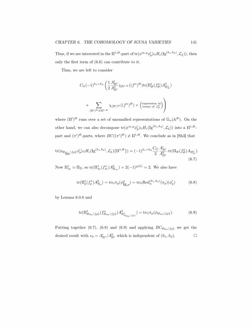
CHAPTER 6. THE COHOMOLOGY OF IGUSA VARIETIES 141
Thus, if we are interested in the Π1,S-part of tr(φ∞,pφ′p|ιlHc(Ig(h1,h2),Lξ)), then
only the first term of (6.6) can contribute to it.
Thus, we are left to consider
CG(−1)h1+h2
(12
A′Π1
A0Π1
χΠ1,S((fn)S)tr(Π1S(fn
S)A0Π1
S)
+∑
(Π′)S +=Π1,S
χ(Π′)S((fn)S)×(
expression interms of fn
S
)
where (Π′)S runs over a set of unramified representations of Gn(AS). On the
other hand, we can also decompose tr(φ∞,pφ′p|ιlHc(Ig(h1,h2),Lξ)) into a Π1,S-
part and (π′)S-parts, where BC((π′)S) "= Π1,S. We conclude as in [Sh3] that
tr(φSfin\{p}φ′p|ιlHc(Ig(h1,h2),Lξ){Π1,S}) = (−1)h1+h2
CG
2A′Π1
A0Π1
·tr(ΠS(fnS)AΠ0
S).
(6.7)
Now Π1∞ * ΠΞ, so tr(Π1
∞(fn∞)A0
Π∞) = 2(−1)q(G) = 2. We also have
tr(Π1p(f
np )A0
Πp) = trιlπp(φn
Ig,p) = trιlRed(h1,h2)
n (πp)(φ′p) (6.8)
by Lemma 6.0.8 and
tr(Π1Sfin\{p}(f
nSfin\{p})A
0Π1
Sfin\{p}) = trιlπp(φSfin\{p}). (6.9)
Putting together (6.7), (6.8) and (6.9) and applying BCSfin\{p} we get the
desired result with e0 = A′Π1/A0Π1 which is independent of (h1, h2).

Chapter 7
Proof of the main theorem
Let E/Q be an imaginary quadratic field in which p splits. Let F1/Q be a
totally real field and let w be a prime of F1 above p. Set F ′ = EF1. Let
F2 be a totally real quadratic extension of Q, in which w = w1w2 splits and
set F = EF2. Let n ∈ Z≥2 . Also denote F2 by F+. Let Π be a cuspidal
automorphic representation of GLn(AF ′).
Consider the following assumptions on (E,F ′, F, Π):
• [F1 : Q] ≥ 2;
• RamF/Q ∪ RamQ(6) ∪ RamQ(Π) ⊂ SplF/F+,Q;
• (Π)∨ * Π ◦ c;
• Π∞ is cohomological for an irreducible algebraic representation Ξ of GLn(F ′⊗Q
C).
• BCF/F ′(Π) is cuspidal
Set Π0 = BCF/F ′(Π) and Ξ0 = BCF/F ′(Ξ). The following lemma is the same
as Lemma 7.2 of [Sh3].
142

CHAPTER 7. PROOF OF THE MAIN THEOREM 143
Lemma 7.0.11. Let Π0 and Ξ0 as above. We can find a character ψ : A×E/E× →
C× and an algebraic representation ξC of G over C satisfying the following con-
ditions
• ψΠ0 = ψc/ψ;
• Ξ0 is isomorphic to the restriction of Ξ′to RF/Q(GLn)×Q C, where Ξ′ is
obtained from ξC by base change from G to Gn;
• ξC|−1E×∞
= ψx∞, and
• RamQ(ψ) ⊂ SplF/F+,Q.
Moreover, if l splits in E then
• ψO×Eu= 1 where u is the place above l induced by ι−1
l τ |E.
Set Π1 = ψ ⊗ Π0. Then Π1 is a cuspidal automorphic representation of
GL1(AE)×GLn(AF ). Let ξ = ιlξC, where ξC is as in Lemma 7.0.11.
Let AU be the universal abelian variety over XU . Since AU is smooth over
XU , Amξ
U satisfies the conditions in Section 4.3. In particular, Amξ
U is locally
etale over a product of strictly semistable schemes. For S, T ⊆ {1, . . . , n}, let
Amξ
U,S,T = Amξ
U ×XU YU,S,T .
Define the following admissible G(A∞,p)-modules with a commuting contin-
uous action of Gal(F ′/F ′):
Hj(XIw(m),Lξ) = lim−→Up
Hj(XU ×F ′ F′,Lξ) = Hj(X,Lξ)Iw(m),
Hj(Amξ
Iw(m), Ql) = lim−→Up
Hj(Amξ
U ×F ′ F′, Ql).
Also define the admissible G(A∞,p)× (FrobF)Z-module
Hj(Amξ
Iw(m),S,T , Ql) = lim−→Up
Hj(Amξ
U,S,T ×F F, Ql).
CHAPTER 7. PROOF OF THE MAIN THEOREM 144
Note that aξ is an idempotent on Hj(Amξ
Iw(m),S,T , Ql(tξ)) and
aξHj+mξ(Amξ
Iw(m),S,T , Ql(tξ)) = Hj(YIw(m),S,T ,Lξ).
Proposition 7.0.12. For each rational prime l "= p there is a G(A∞,p) ×
(FrobF)Z-equivariant spectral sequence with a nilpotent operator N
BCp(Ei,m+mξ−i1 (Iw(m), ξ)[Π1,S]) ⇒
BCp(WD(Hm(XIw(m),Lξ)|Gal(K/K)[Π1,S])F−ss),
where
BCp(Ei,m+mξ−i1 (Iw(m), ξ)[Π1,S]) =
⊕
k−l=−i
BCp(aξHm+mξ(Amξ
Iw(m),GrlGrkRψQl(tξ))[Π1,S]).
The action of N sends BCp(aξHm+mξ(Amξ
Iw(m),GrlGrkRψQl(tξ))[Π1,S]) to
BCp(aξHm+mξ(Amξ
Iw(m),Grl+1Grk−1RψQl(tξ))[Π1,S]).
Furthermore, there is a direct sum decomposition
BCp(aξHm+mξ(Amξ
Iw(m),GrlGrkRψQl(tξ))[Π1,S]) *⊕
j≥0
BCp(Mj,m+mξ−j(k, l)),
where
BCp(Mj,m+mξ−j(k, l)) =k+l⊕
s=1
⊕
#S=j+s,#T=j+k+l−s+1
Hj+mξ,sS,T (k, l)
CHAPTER 7. PROOF OF THE MAIN THEOREM 145
and
Hj+mξ,sS,T (k, l) = BCp(aξH
m+mξ−2j−k−l+1(Amξ
Iw(m),S,T , Ql(tξ− j−k +1))[Π1,S])
= BCp(Hm−2j−k−l+1(YIw(m),S,T , Ql(−j − k + 1))[Π1,S]).
Proof. Note that Amξ
U /OK satisfies the hypotheses of Section 4. We have a
spectral sequence of G(A∞,p)× (FrobF)Z-modules with a nilpotent operator N :
Ei,m−i1 (Iw(m), ξ) ⇒ Hm(Amξ
U ×F ′ F′p, Ql(t)),
where
Ei,m−i1 (Iw(m), ξ) =
⊕
k−l=−i
Hm(Amξ
U ×F F, GrlGrkRψQl(t)).
N will send Hm(Amξ
U ,GrlGrkRψQl(t)) to Hm(Amξ
U ,Grl+1Grk−1RψQl(t)).
By Corollary 4.3.10, we also have a G(A∞,p)× (FrobF)Z-equivariant isomor-
phism
Hm(Amξ
U ×F F, GrlGrkRψQl(t)) *⊕
j≥0
Mj,m−j(k, l)
where
Mj,m−j(k, l) =k+l⊕
s=1
⊕
#S=j+s#T=j+k+l−s+1
Hj,sS,T (k, l)
and
Hj,sS,T (k, l) = Hm−2j−k−l+1(Amξ
U,S,T ×F F, Ql(t− j − k + 1)).
We take t = tξ, apply aξ, replace j by j + mξ and take the inverse limit over
Up. We get a spectral sequence of G(A∞,p)× (FrobF)Z-modules, converging to
Hj(XIw(m),Lξ). We identify Hj(XIw(m),Lξ) with its associated Weil-Deligne
representation and we semisimplify the action of Frobenius. After taking Π1,S-
CHAPTER 7. PROOF OF THE MAIN THEOREM 146
isotypical components and applying BCp we get the desired spectral sequence.
Corollary 7.0.13. Keep the assumptions made in the beginning of this section.
The Weil-Deligne representation
WD(BCp(H2n−2(XIw(m),Lξ)|Gal(K/K)[Π1,S]))F−ss
is pure of weight mξ − 2tξ + 2n− 2.
Proof. By Proposition 5.3.5,
BCp(Hj(YIw(m),S,T ,Lξ)[Π1,S]) = 0
unless j = 2n−#S −#T . Thus, the terms of the direct sum decomposition
BCp(Mj,m+mξ−j(k, l)),
which are all of the form
BCp(Hm−2j−k−l+1(YIw(m),S,T , Ql(−j − k + 1))[Π1,S])
with #S = j + s and #T = j + k + l − s + 1, vanish unless m = 2n − 2. This
means that the terms of the spectral sequence BCp(Ei,m+mξ−i1 (Iw(m), ξ)[Π1,S])
vanish unless m = 2n− 2. If m = 2n− 2 then each summand of
BCp(Ei,2n−2+mξ−i1 (Iw(m), ξ)[Π1,S])
has a filtration with graded pieces
BCp(H2n−2−2j−k−l+1(YIw(m),S,T ,Lξ(−j − k + 1))[Π1,S]),

CHAPTER 7. PROOF OF THE MAIN THEOREM 147
where k − l = −i. These graded pieces are strictly pure of weight mξ − 2tξ +
2n− 2 + k − l − 1, which only depends on i. Thus, the whole of
BCp(Ei,2n−2+mξ−i1 (Iw(m), ξ)[Π1,S])
is strictly pure of weight mξ − 2tξ + 2n − 2 − i − 1. The spectral sequence
degenerates at E1, since Ei,m−i1 = 0 unless m = 2n − 2 and also the abutment
is pure of weight mξ − 2tξ + 2n− 2. Thus,
BCp(WD(Hm(XIw(m),Lξ)|Gal(K/K)[Π1,S])F−ss)
vanishes for m "= 2n−2 and is pure of weight mξ−2tξ+2n−2 for m = 2n−2.
Theorem 7.0.14. Let n ∈ Z≥2 be an integer and L be any CM field. Let l be a
prime and ιl be an isomorphism ιl : Ql → C. Let Π be a cuspidal automorphic
representation of GLn(AL) satisfying
• Π∨ * Π ◦ c
• Π is cohomological for some irreducible algebraic representation Ξ.
Let
Rl(Π) : Gal(L/L) → GLn(Ql)
be the Galois representation associated to Π by [Sh3, CH]. Let p "= l and let y be
a place of L above p. Then we have the following isomorphism of Weil-Deligne
respresentations
WD(Rl(Π)|Gal(Ly/Ly))F−ss * ι−1
l Ln,Ly (Πy).
Proof. This theorem has been proven by [Sh3] except in the case when n is even
and Ξ is not slightly regular. In that exceptional case it is still known that

CHAPTER 7. PROOF OF THE MAIN THEOREM 148
we have an isomorphism of semisimplified WLy -representations by [CH], so it
remains to check that the two monodromy operators N match up. By Corollary
5.3.4, Πy is tempered. This is equivalent to ι−1l Ln,Ly (Πy) being pure of weight
2n−2. In order to get an isomorphism of Weil-Deligne representations, it suffices
to prove that WD(Rl(Π)|Gal(Ly/Ly))F−ss is pure.
We first will find a CM field F ′ such that
• F ′ = EF1, where E is an imaginary quadratic field in which p splits and
F1 = (F ′)c=1 has [F1 : Q] ≥ 2,
• F ′ is soluble and Galois over L,
• Π0F ′ = BCF ′/L(Π) is a cuspidal automorphic representation of GLn(AF ′),
and
• there is a place p of F above y such that Π0F ′,p has an Iwahori fixed vector,
and a CM field F which is a quadratic extension of F ′ such that
• p = p1p2 splits in F ,
• RamF/Q ∪ RamQ(6) ∪ RamQ(Π) ⊂ SplF/F ′,Q, and
• Π0F = BCF/F ′(Π0
F ′) is a cuspidal automorphic representation of GLn(AF ).
To find F and F ′ we proceed as in the proof of Corollary 5.3.4. Set Π1F = Π0
F⊗ψ,
where ψ is chosen as in Lemma 7.0.11.
We claim that we have isomorphisms
CG · (Rl(Π)|Gal(F ′/F ′))⊗2 * CG ·Rl(Π0
F ′)⊗2 * R2n−2
l (Π1F )⊗Rl(ψ)−1,
where Rkl (Π1
F ) was defined in Section 4. The first isomorphism is clear. The
second isomorphism can be checked by Chebotarev locally at unramified places,

CHAPTER 7. PROOF OF THE MAIN THEOREM 149
using the local global compatibility for Rl(Π0F ′) and the formula
Rl(Π1F ) = e0CG · [(πp,0 ◦Art−1
Qp)|WF ′p
⊗ ι−1l LF ′p,n(Π0
F ′,p)⊗2].
(It can be checked easily, either by computing the weight or by using the spectral
sequences above that Rkl (Π1
F ) "= 0 if and only if k = 2n − 2 and thus that
e0 = (−1)2n−2 = 1.)
We also have
BCp(H2n−2(XIw(m),Lξ)[Π1,SF ]) * (dimπIw(m)
p ) · ι−1l Π∞,p ⊗ R2n−2(Π1
F )
as admissible representations of G(A∞,p) × Gal(F ′/F ′). By Corollary 7.0.13,
WD(R2n−2l (Π1
F )|Gal(F ′p/F ′p)) is pure of weight mξ− 2tξ +2n− 2. By Lemma 1.7
of [TY],
WD(Rl(Π0F ′)
⊗2|Gal(F ′p/F ′p))
is also pure. It has weight 2n−2. The monodromy operator acts on Rl(Π0F ′)⊗2|WF ′p
as 1⊗N +N⊗1, where N is the monodromy operator on Rl(Π0F ′)|WF ′p
. We wish
to show that V := WD(Rl(Π0F ′)|WF ′p
)F−ss is pure of weight n − 1. Consider
the direct sum decomposition V = ⊕i∈ZVi, where Vi is strictly pure of weight
n − 1 + i. It suffices to prove that N i : Vi → V−i is injective for every i > 0,
since then we can compare dimensions to deduce that N i is an isomorphism.
Let x ∈ Vi and assume that N ix = 0. Since x ∈ Vi, the vector x ⊗ x belongs
to the subspace of WD(Rl(Π0F ′)⊗2|WF ′p
)F−ss which is strictly pure of weight
2n− 2 + 2i. But then
N2i(x⊗ x) =2i∑
k=0
Nkx⊗N2i−kx = 0,
which contradicts the purity of WD(Rl(Π0F ′)⊗2|WF ′p
)(F−ss). Thus, WD(Rl(Π0F ′)|Gal(F ′p/F ′p))F−ss
CHAPTER 7. PROOF OF THE MAIN THEOREM 150
has to be pure. By Lemma 1.4 of [TY], purity is preserved under finite exten-
sions, so WD(Rl(Π)|Gal(Ly/Ly))F−ss is also pure.

Bibliography
[AC] Arthur, J. and Clozel, L.: Simple algebras, base change, and the advanced
theory of the trace formula, Princeton University Press, no. 120, Ann. of
Math. Studies, Princeton, New Jersey (1989).
[Art] Arthur, J.: The invariant trace formula II, Global theory, J. Amer. Math.
Soc. 1 (1988), 501-554.
[Bad] Badulescu, A.I.: Jacquet-Langlands et unitarisabilite, J. Inst. Math.
Jussieu 6 (2007), 349-379.
[BLGGT1] Barnet-Lamb, T., Gee, T., Geraghty, D. and Taylor, R: Local-global
compatibility for l = p, I, preprint (2011).
[BLGGT2] Barnet-Lamb, T., Gee, T., Geraghty, D. and Taylor, R: Local-global
compatibility for l = p, II, preprint (2011).
[Be] Beilinson, A.A.: On the derived category of perverse sheaves, in K-theory,
arithmetic and geometry (Moscow, 1984-1986) Lecture Notes in Math.,
1289, Springer Berlin, (1987), 27-41.
[BBD] Beilinson, A.A., Bernstein, J. and Deligne, P.: Faisceaux pervers, Aster-
isque 100, SMF (1982).
151

BIBLIOGRAPHY 152
[BZ] Bernstein, I.N and Zelevinsky, A.V.: Induced representations of reductive
p-adic groups I, Ann. Sci. ENS (4) 10 (1997), 441-472.
[Bor] Borel, A.: Automorphic L-functions, pp. 27-61 in Borel and Casselman
(eds.): Automorphic forms, representations and L-functions, Proc. of Symp.
in Pure Math., vol. 33.2, Providence, RI, AMS, Amer. Math. Soc., 1979.
[Car] Caraiani, A.: Local-global compatibility and monodromy for l = p,
preprint, arXiv:1202.4683.
[CH] Chenevier, G. and Harris, M.: Construction of automorphic Galois repre-
sentations, II, http://people.math.jussieu.fr/~harris/ConstructionII.pdf.
[Cl1] Clozel, L.: Representations galoisiennes associes aux representations au-
tomorphes autoduales de GL(n), Publ. Math. I.H.E.S. 73 (1991), 97-145.
[Cl2] Clozel, L.: Purity reigns supreme, http://fa.institut.math.jussieu.fr/node/45.
[De1] Deligne, P.: La conjecture de Weil I, Inst. Hautes Etudes Sci. Publ. Math.
43 (1974), 273-307.
[De2] Deligne, P.: La conjecture de Weil II, Inst. Hautes Etudes Sci. Publ.
Math. 52 (1980), 137-252.
[D] Drinfeld, V. G.: Elliptic modules, Math. USSR Sbornik 23 (1974), no. 4,
561-592.
[EGA3] Grothendieck, A. and Dieudonne, J.: Elements de geometrie algebrique
III. Etude cohomologique des faisceaux coherents, Seconde partie, Publ.
Math. I.H.E.S. 17 (1963), 5-91.
[EGA4] Grothendieck, A and Dieudonne, J.: Elements de geometrie algebrique
IV. Etude locale des schemas et des morphismes de schemas, Quatrieme
partie, Publ. Math. I.H.E.S. 32 (1967), 5-361.

BIBLIOGRAPHY 153
[E] Ekedahl, T.: On the adic formalism, in The Grothendieck Festschrift Vol-
ume II, Progress in Math, Birkhauser 87, (1990), 197-218.
[HT] Harris, M. and Taylor, R.: The geometry and cohomology of some simple
Shimura varieties, Princeton University Press, no. 151, Annals of Math.
Studies, Princeton, New Jersey (2001).
[I1] Illusie, L.: An overview of the work of K. Fujiwara, K. Kato, and C.
Nakayama on logarithmic etale cohomology, Cohomologies p-adiques et ap-
plications arithmetiques (II), Asterisque 279 (2002), 271-322.
[I2] Illusie, L.: Autour du theoreme de monodromie locale, Periodes p-adiques,
Asterisque 223 (1994), 9-58.
[K] Kato, K.: Logarithmic structures of Fontaine-Illusie.
[KN] Kato, K. and Nakayama, C.: Log Betti cohomology, log etale cohomology,
and log de Rham cohomology of log schemes over C, Kodai. Math. J. 22
(1999), 161-186.
[KM] Katz, N and Mazur, B.: Arithmetic moduli of elliptic curves, Princeton
University Press 1985.
[Ko1] Kottwitz, R.: Points on some Shimura varieties over finite fields, Jour. of
the AMS 5 (1992), 373-444.
[Ko2] Kottwitz, R: On the λ-adic representations associated to some simple
Shimura varieties, Invent. Math. 108 (1992), 653-665.
[Lan] Lan, K.-W.: Arithmetic compactifications of PEL-type Shimura varieties,
Harvard thesis (2008).
[Man] Mantovan, E.: On the cohomology of certain PEL-type Shimura varieties,
Duke Math. 129 (2005), 573-610.
BIBLIOGRAPHY 154
[Na] Nakayama, C.: Nearby cycles for log smooth families, Comp. Math. 112
(1998), 45-75.
[O] Ogus, A.: Relatively coherent log structures, Preprint.
[Ra] Ramanujan, S.: On certain arithmetical functions, Transactions of the
Cambridge Philosophical Society XXII (9) (1916), 159–184. Reprinted in
Ramanujan, S.: (2000), "Paper 18", Collected papers of Srinivasa Ramanu-
jan, AMS Chelsea Publishing, Providence, RI, pp. 136–162.
[RZ] Rapoport, M. and Zink, Th.: Uber die lokale Zetafunktion von Shimu-
ravarietaten. Monodromiefiltration und verschwindende Zyklen in ungle-
icher Charakteristik, Invent. Math. 68 (1982), 21-101.
[Re] Reich, R.: Notes on Beilinson’s “How to glue perverse sheaves”,
arXiv:math.AG/1002.1686v1.
[Sa1] Saito, M.: Modules de Hodge polarisables, Publ. RIMS 24 (1988), 849-
995.
[Sa2] Saito, T.: Weight spectral sequences and independence of l, Journal of
the Inst. Math. Jussieu (2003) 2(4), 583-634.
[Sar] Sarnak, P.: Notes on the generalized Ramanujan conjectures, in Arthur,
J., Elwood, D. and Kottwitz, R.: Harmonic analysis, the trace formula, and
Shimura varieties, Clay Math. Proc. 4 (2005), Providence, RI, Am. Math.
Soc., 659-685.
[She] Shelstad, D.: L-indistinguishability for real groups, Math. Ann. 259
(1982), 385-430.
[Sh1] Shin, S. W.: Counting points on Igusa varieties, Duke Math. 146 (2009),
509-568.

BIBLIOGRAPHY 155
[Sh2] Shin, S.W.: Stable trace formula for Igusa varieties, J. Inst. Math. Jussieu
9 (4), (2010), 847-895.
[Sh3] Shin, S. W.: Galois representations arising from some compact Shimura
varieties, preprint (2009), to appear in Ann. of Math.
[SGA4] Artin, M., Grothendieck, A. and Verdier, J.-L.: Theorie des topos et
cohomologie etale des schemas, Lect. Notes Math. 305 (1972).
[SGA7] Grothendieck, A., Deligne, P. and Katz, N., with Raynaud, M. and
Rim, D. S.: Groupes de monodromie en geometrie algebriques, Lect. Notes
Math. 288, 340 (1972-73).
[Tad] Tadic, M.: Classification of unitary representations in irreducible repre-
sentations of general linear group (non-archimeadean case), Ann. Sci. E.N.S.
19 (1986), 335-382.
[Tat] Tate, J.: Classes d’isogenie des varietes abeliennes sur un corps fini, Sem-
inaire Bourbaki 352, Lect. Notes Math. 179 (1971).
[TY] Taylor, R. and Yoshida, T.: Compatibility of local and global Langlands
correspondences, J. Amer. Math. Soc. 20 (2) (2007), 467-493.
[Y] Yoshida, T.: On non-abelian Lubin-Tate theory via vanishing cycles, to
appear in Adv. Stud. in Pure Math.


![Jumps and Monodromy of Abelian Varieties · Communicated by Peter Schneider Abstract. We prove a strong form of the motivic monodromy conjecture for abelian varieties, ... [14], this](https://img.dokumen.tips/doc/110x75/60cb52adf18c43607b1299a3/jumps-and-monodromy-of-abelian-varieties-communicated-by-peter-schneider-abstract.jpg)


![Action Research (Bagian Proposal PTK-1) [Compatibility Mode]](https://img.dokumen.tips/doc/110x75/588073c61a28ab7c108bb2e3/action-research-bagian-proposal-ptk-1-compatibility-mode.jpg)

