Embed Size (px)
Citation preview

Local discrete velocity grids for deterministic rarefied flow simulations
S. Brull1, L. Mieussens2
1Univ. Bordeaux, IMB, UMR 5251, F-33400 Talence, France.CNRS, IMB, UMR 5251, F-33400 Talence, France.
2Univ. Bordeaux, IMB, UMR 5251, F-33400 Talence, France.CNRS, IMB, UMR 5251, F-33400 Talence, France.
INRIA, F-33400 Talence, France.([email protected])
Abstract
Most of numerical methods for deterministic simulations of rarefied gas flows usethe discrete velocity (or discrete ordinate) approximation. In this approach, the kineticequation is approximated with a global velocity grid. The grid must be large and fineenough to capture all the distribution functions, which is very expensive for high speedflows (like in hypersonic aerodynamics). In this article, we propose to use insteaddifferent velocity grids that are local in time and space: these grids dynamically adaptto the width of the distribution functions. The advantages and drawbacks of themethod are illustrated in several 1D test cases.
Keywords: kinetic equations, discrete velocity model, deterministic method, rarefied gas dy-namics
1 Introduction
Most of deterministic numerical methods for rarefied flow simulations are based on a discretevelocity approximation of the Boltzmann equation, see for instance [25, 23, 8, 7, 6, 19, 20,16, 26, 14].
In almost all these methods, the distribution function is approximated with a globalvelocity grid, for every point in the position space, for every time. This makes the methodrobust (conservation, entropy dissipation, positivity, stability, etc.) and relatively simple,but very expensive for many cases. Indeed, the grid must be large enough to contain all thedistribution functions of the flow, and fine enough to capture every narrow distributions. Thefirst constraint makes the grid very large for high speed flow with large temperatures. Thesecond constraint makes the grid step very small, and hence a very large number of discretevelocities are needed. This is for instance the case for atmospheric re-entry problems, wherethe flow is hypersonic. These problems, especially in 3D, are very difficult to be simulated
1

with such methods, due to the discrete velocity grid that contains a prohibitively largenumber of points.
Of course, particle solvers like the popular Direct Simulation Monte-Carlo method (DSMC)do not suffer of such problems [5]. However, if one is interested in deterministic Euleriansimulations, it is important to find a way to avoid the use of a too large number of dis-crete velocities. Up to our knowledge, there are a few papers on this subject. Aristovproposed in [1] an adaptive velocity grid for the 1D shock structure calculation. However,the approach is very specific to this test case and has never been extended. More recently,Filbet and Rey [12] proposed to use a rescaling of the velocity variable to make the supportof the distribution independent of the temperature and of the macroscopic velocity. Thenthe Boltzmann equation is transformed into a different form (with inertia terms due to thechange of referential). In [2], Baranger et al. proposed an algorithm to locally refine thevelocity grid wherever it is necessary and to coarsen it elsewhere. But this approach, whichhas been proved to be very efficient for steady flows, is still based on a global grid, andcannot be efficient enough for unsteady flows. Finally, Chen et al. [9] proposed to use adifferent velocity grid for each point in the position space and every time: from one point toanother one, the grid is refined or coarsen by using an Adaptive Mesh Refinement (AMR)technique. This seems to be very efficient, but all the grids have the same bounds (they alluse the same background grid). It seems that a similar method was proposed at the sametime by Kolobov et al., see [17, 15].
In this paper, we propose a method that has several common features with the methodof [27] and [12] but is still very different. The main difference is that each distribution isdiscretized on its own velocity grid: each grid has its own bounds and step that are evolved intime and space by using the local macroscopic velocity and temperature. These macroscopicquantities are estimated by solving the local conservation laws of mass, momentum, andenergy. The interaction between two space cells requires to use reconstruction techniques toapproximate a distribution on different velocity grids. This paper is a preliminary work, for1D flows, that proposes a complete algorithmic approach. Several test cases illustrate theproperties of the method and show its efficiency.
The outline of the paper is the following. In section 2 is presented a simple 1D kineticBhatnagar-Gross-Krook (BGK) model and its standard discrete velocity approximation. Insection 3, the local discrete velocity grid approach is described. The numerical tests aregiven in section 4.
2 A simple 1D kinetic model and its standard velocity
discretization
We consider a one-dimensional gas described by the mass density of particles f(t, x, v) thatat time t have the position x and the velocity v (note that both position x and velocity v arescalar). The corresponding macroscopic quantities can be obtained by the moment vectorU(t, x) = 〈mf(t, x, .)〉, where m(v) = (1, v, 1
2|v|2) and 〈φ〉 =
∫
Rφ(v) dv for any velocity
2

dependent function. This vector can be written component wise by U = (ρ, ρu, E), where ρ,ρu, and E are the mass, momentum, and energy densities. The temperature T of the gas isdefined by relation E = 1
2ρ|u|2 + 1
2ρRT , where R is the gas constant.
The evolution of the gas is governed by the following BGK equation
∂tf + v∂xf =1
τ(M(U)− f), (1)
where M(U) is the local Maxwellian distribution defined through the macroscopic quantitiesU of f by
M(U) =ρ√
2πRTexp
(
−|v − u|22RT
)
, (2)
and τ = CT ω/ρ is the relaxation time. The constant C and ω will be given in section 4 foreach test case.
From this equation, it is easy to establish the so called conservation laws that describethe time evolution of the moment vector U :
∂tU + ∂x 〈vmf〉 = 0. (3)
For the numerical approximation of equation (1), a popular method is the discreteordinate–or discrete velocity–method. It consists in choosing a grid V of K points vk, andthen in replacing the kinetic equation (1) by the finite set of K equations
∂tfk + vk∂xfk =1
τ(Mk(U)− fk) (4)
where fk(t, x) is an approximation of f(t, x, vk) andMk(U) is an approximation ofM(U)(vk).This approximation is the discrete Maxwellian whose parameters are such that it has thesame discrete moments as the distribution f , as proposed in [18, 19]. This gives a conservativediscrete velocity model.
In order to describe the solution correctly, the discrete velocity grid V must captureall the distribution functions, that is to say at any time t, and for every position x. Thismeans that V must be large enough to capture distributions with large mean velocity orlarge temperature, and fine enough to capture distributions with small temperature. Seean illustration of this problem in figure 1. In this figure, we show a 2D aerodynamical flowwith three typical distributions functions (one in the upstream flow, one in the shock, andanother one at the boundary). The corresponding velocity grid is shown in the same figure.
To construct such a grid, we start with a remark on the local Maxwellians. Since aMaxwellian centered on u and of temperature T decreases very fast for large v, it is verysmall outside any interval [u− c
√RT, u+ c
√RT ] with c sufficiently large. A good choice for
such an interval is obtained with c = 3√RT : as it is well know in statistics for the normal
distribution, 99% of the particles described by the local Maxwellian have their velocity inthis interval. For kinetic simulations, we generally take a slightly larger interval with c = 4.The corresponding interval [u − 4
√RT, u + 4
√RT ] is what we call the “support” of the
3

local Maxwellian and contains the “essential” information on the distribution. When adistribution is not too far from its corresponding local Maxwellian (which is true when theKnudsen number is not too small, away from shock and boundary layers), most of particlesdescribed by this distribution have their velocity localized in the support of the correspondinglocal Maxwellian. This is interesting, since this support can be analytically determined as afunction of the macroscopic velocity and temperature, as it has been shown above.
Consequently, a first constraint for the global velocity grid is that its bounds vmin andvmax satisfy the following inequalities:
vmin ≤ mint,x
(
u(t, x)− 4√
RT (t, x))
, vmax ≥ maxt,x
(
u(t, x) + 4√
RT (t, x))
, (5)
so that all the distributions can be captured in the grid. Since it is reasonable to requirethat there are at least three points between the inflexion points of any Maxwellian, the stepof the global grid should be such that
∆v ≤ mint,x
√
RT (t, x). (6)
Of course, such an approach requires to first estimate some bounds on the macroscopic fieldsthat are global in time and space.
Note that the points of V are not necessarily uniformly distributed, since the grid couldbe refined only wherever it is necessary and coarsened elsewhere, as it is proposed in [3] forsteady flows (with a simple and automatic way to define such a grid). However, for unsteadyproblems, the situation is more complex. Indeed, first, the estimations of the correct boundsand step of the grid are not necessarily available for every problems (the velocity or thetemperature could reach much larger values that were not expected at some times of thesimulation), like in complex shock interactions, for instance. Moreover, even if it is possible,this could lead to a grid which is extremely large and dense, hence leading to a very expensivesimulation (see an example in section 4.2). Finally, when there are distributions that arevery far from their local Maxwellian, their support can be quite different, and there is noanalytical way to determine it. This can require several tries to find a correct global velocitygrid, which is also expensive.
It is therefore very attractive to try to use a local velocity discretization of the distributionfunction, which means to use local discrete velocity grids (LDV) for each time and position.In other words, at each time t and position x, we would like the corresponding distributionf(t, x, .) to be approximated on its own velocity grid, which might be different from the gridsused at other times or other positions. The clear advantage of this idea is that we can definean optimally small grid for each distribution, thus we avoid the problems mentioned above.This approach is developed in the next section.
4

3 A local discrete velocity grid approach
3.1 The method
Now we assume that at time tn, the distribution function in each space cell [xi− 1
2
, xi+ 1
2
] isapproximated on a set Vn
i of K local discrete velocities. For simplicity, we assume herethat all the local grids have the same number of points K, and the points are uniformlydistributed. The first point is denoted by vnmin,i and the last one by vnmax,i. That is to say,we have
Vni =
{
vni,k = vnmin,i + (k − 1)∆vni , k from 1 to K}
, where ∆vni =vnmax,i − vnmin,i
K − 1.
On this local grid, f(tn, xi, .) is approximated by K values that are stored in the vectorfni = (fn
i,k)Kk=1. Each discrete value fn
i,k is an approximation of f(tn, xi, vni,k).
The corresponding macroscopic quantities U(tn, xi) are approximated by Uni with the
following quadrature formula
Uni = 〈mfn
i 〉Vn
i
=K∑
k=1
m(vni,k)fni,kωk, (7)
where the ωk are the weights of the quadrature. In this paper, the trapezoidal quadratureformula is used: ω1 = ωK = 1/2 and ωk = 1 for k from 2 to K − 1.
When one wants to compute an approximation of f at the next time step tn+1, twoproblems occur. First, how to determine the local discrete velocity grid Vn+1
i ? We will showbelow that this can be simply made by using the conservation laws. Second, how to exchangeinformation between two space cells, since the local grids are not the same? This is wherewe use some interpolation procedure in the method. Let us now describe our algorithm stepby step.
Step 1: Macroscopic quantities at tn+1.
We approximate the conservation relation (3) with the following first order upwind scheme
Un+1i = Un
i − ∆t
∆x
(
Φni+ 1
2
− Φni− 1
2
)
, (8)
where the numerical fluxes are defined by
Φni+ 1
2
=⟨
v+mfni
⟩
Vn
i
+⟨
v−mfni+1
⟩
Vn
i+1
, (9)
which is indeed an approximation of the flux⟨
vmf(tn, xi+ 1
2
)⟩
at the cell interface. Here,
we use the standard notation v± = (v ± |v|)/2. Note that each half flux is computed on thelocal velocity grid of the corresponding distribution. The vector Un+1
i is an approximationof U(tn+1, xi), and we note un+1
i and T n+1i the corresponding velocity and temperature.
5

Step 2: discrete velocity grid Vn+1i .
We define this grid by using the new velocity and temperature un+1i and T n+1
i to get thebounds
vn+1min,i = un+1
i − 4√
RT n+1i and vn+1
max,i = un+1i + 4
√
RT n+1i . (10)
Then the new grid Vn+1i is defined as in the previous time step, that is to say by
Vn+1i = {vn+1
i,k = vn+1min,i + (k − 1)∆vn+1
i , k from 1 to K},with ∆vn+1
i = (vn+1max,i − vn+1
min,i)/(K − 1).(11)
Step 3: distribution function at time tn+1.
Here, equation (1) is approximated by a first order upwind scheme, with an implicitrelaxation term. If the velocity variable is not discretized, we get for every v:
fn+1i (v) = fn
i (v)−∆t
∆xv+(fn
i (v)− fni−1(v))−
∆t
∆xv−(fn
i+1(v)− fni (v))
+∆t
τn+1i
(M(Un+1i )(v)− fn+1
i (v)).
If now we take into account that each distribution fn+1i , fn
i , fni−1, and fn
i+1 are defined on theirown local velocity grid, this scheme must be modified by using a reconstruction procedure.
The discrete distributions fni , f
ni−1, and fn
i+1 are used to reconstruct piecewise continuousin velocity functions fn
i , fni−1, and fn
i+1 that are defined as follows:
fni (v) =
{
pni (v) if vnmin,i ≤ v ≤ vnmax,i
0 else,(12)
where pni is a piecewise continuous function of v constructed through the values (vni,k, fni,k)
Kk=1,
like a piecewise interpolated polynomial. Since any kind of interpolation could be used, thisreconstruction will be discussed in section 3.3. Then we define the discrete values of fn+1
i
on its grid Vn+1i by
fn+1i,k = fn
i (vn+1i,k )− ∆t
∆xvn+1i,k
+(fn
i (vn+1i,k )− fn
i−1(vn+1i,k ))− ∆t
∆xvn+1i,k
−(fn
i+1(vn+1i,k )− fn
i (vn+1i,k ))
+∆t
τn+1i
(Mk(Un+1i )− fn+1
i,k ),
(13)
for k = 1 to K.Our scheme is then given by relations (8–13). Now, we give some properties of this
scheme.
Property 3.1. For scheme (8–13), the global mass, momentum, and energy are constant(the scheme is conservative):
∑
i
Uni ∆x =
∑
i
U0i ∆x.
6

Proof. This is a direct consequence of the discretization of the conservation laws (8) witha conservative scheme: indeed, when we take the sum of (8) for every i, the sum of thenumerical fluxes cancels out, and we obtain that the total quantities do not change duringone time step. This gives the result.
Even if this property is obvious, we believe it deserves to be noted: first, we point outthat the scheme is not given by (8) only, but by all the relations between (8) and (13). Thenrelation (8) has to be seen as macroscopic conservation laws in which the fluxes are computedby using the discrete kinetic equation (13). Even if (13) is not conservative, the use of (8)implies that the macroscopic mass, momentum, and energy densities are conserved. This isa property shared by several recent schemes based on a dual macro-micro time evolutions orIMEX methods, see for instance [21, 4, 11].
Property 3.2. Assume that for every cell i, fni is non negative at each point of its local
velocity grid and that the corresponding reconstructed piecewise function fni is non negative
for every v. Then, under the CFL condition ∆t ≤ ∆x/maxi,k(|vn+1i,k |), fn+1
i,k is non negativeat each point of its local velocity grid, for every space cell.
Proof. As it is standard for the upwind scheme for convection problems, it is sufficient tonote that (13) can be written as a linear combination of fn
i , fni−1, f
ni+1, and M(Un+1
i ). TheCFL condition of the proposition ensures that the coefficients of this combination are nonnegative, which gives the result.
We point out that, while the result of this property is rather standard, it is in factquite weak here. Indeed, first, the non negativeness of the distribution is obtained only ifthe reconstruction step preserves the non negativeness of the fn
i . This is true for linearinterpolation, but it is not for many higher order reconstructions. Moreover, this propertyitself is not sufficient to ensure that the sequence fn
i can be defined at every time step:indeed, step 2 requires T n+1
i to be non-negative to define the local grid Vn+1i . Unfortunately,
it seems hardly possible to prove that this property is true for the scheme presented above.This why a modified schemes are presented in the next section.
Finally, we want to comment on the choice of the time step in this scheme. Indeed, notethat, according to property 3.2, step 3 requires a time step defined through the local gridsVn+1i at time tn+1 to correctly define fn+1
i . However, this time step is already needed at step1 to define Un+1
i , while at this step, Vn+1i is not already known. This means that we have to
use a single time step for steps 1 and 3 that also satisfies the CFL condition based on Vn+1i .
A simple algorithm is the following:
(a) We choose ∆t1 = ∆x/maxi,k(|vni,k|)
(b) We do step 1 and step 2.
(c) For step 3, we compute ∆t2 = ∆x/maxi,k(|vn+1i,k |):
• if ∆t2 > ∆t1, then fn+1 can be advanced with ∆t1
7

• if ∆t2 < ∆t1, then we set ∆t1 = ∆t2, we do not compute fn+1 but we directly goback to (b) (steps 1 and 2 of the scheme are done again)
However, note that in practice, we do not need this algorithm: we always use ∆t1 =∆x/maxi,k(|vni,k|) without any stability problem. Indeed, we carefuly checked the sign ofthe solution at each time step and at every space and velocity point, for all the test casespresented in this paper: we did not observe any loss of positivity and any stability problem.
3.2 Modified versions of the scheme
First, note that if we compute the moments of fn+1i after step 3, we do not recover the
moments Un+1i defined at step 1. Indeed, according to (13) we have
⟨
mfn+1i
⟩
Vn+1
i
=∑
Vn+1
i
m(vn+1i,k )fn+1
i,k ωk
=∑
Vn+1
i
m(vn+1i,k )fn
i (vn+1i,k )ωk −
∆t
∆x
∑
Vn+1
i
m(vn+1i,k )(vn+1
i,k
+fni (v
n+1i,k ) + vn+1
i,k
−fni+1(v
n+1i,k ))ωk
−∑
Vn+1
i
m(vn+1i,k )(vn+1
i,k
+fni−1(v
n+1i,k )− vn+1
i,k
−fni (v
n+1i,k ))ωk
+∆t
τn+1i
(
Un+1i −
⟨
mfn+1i,k
⟩
Vn+1
i
)
.
If we compare the terms of this expression to the definition of Un+1i given by (8) and (9),
we find the two vectors cannot be equal. The reason is that in the first expression, we haveseveral quantities on the form
∑
Vn+1
i
φ(vn+1i,k )fn
i (vn+1i,k )ωk, while in the second expression,
these quantities are∑
Vn
i
φ(vni,k)fni,kωk, and they are not equal in general since the grids Vn+1
i
and Vni are different. Of course, these quantities are close, since they approximate the same
values, but they are not equal.This means that we have two different approximations of the same macroscopic values:
Un+1i and the moments of fn+1
i . We have numerically compared these quantities and thereis indeed no significant difference. However, this difference suggests a modification of thescheme: after step 3, we add one more step in which we define Un+1,⋆
i =⟨
mfn+1i
⟩
Vn+1
i
, and
Uni is replaced by Un,⋆
i in step 1. Then the modified scheme (called the “moment correctionmethod”) is the following:
Step 1: Macroscopic quantities at tn+1.
Un+1i = Un,⋆
i − ∆t
∆x
(
Φni+ 1
2
− Φni− 1
2
)
, (14)
8

where the numerical fluxes are defined by
Φni+ 1
2
=⟨
v+mfni
⟩
Vn
i
+⟨
v−mfni+1
⟩
Vn
i+1
, (15)
Step 2: discrete velocity grid Vn+1i (step unchanged).
vn+1min,i = un+1
i − 4√
RT n+1i and vn+1
max,i = un+1i + 4
√
RT n+1i . (16)
Vn+1i = {vn+1
i,k = vn+1min,i + (k − 1)∆vn+1
i , k from 1 to K},with ∆vn+1
i = (vn+1max,i − vn+1
min,i)/(K − 1).(17)
Step 3: distribution function at time tn+1 (step unchanged).
fn+1i,k = fn
i (vn+1i,k )− ∆t
∆xvn+1i,k
+(fn
i (vn+1i,k )− fn
i−1(vn+1i,k ))− ∆t
∆xvn+1i,k
−(fn
i+1(vn+1i,k )− fn
i (vn+1i,k ))
+∆t
τn+1i
(Mk(Un+1i )− fn+1
i,k ),
(18)
for k = 1 to K.
Step 4: Moment correction step.
Un+1,⋆i =
⟨
mfn+1i
⟩
Vn+1
i
=K∑
k=1
m(vn+1i,k )fn+1
i,k ωk. (19)
This means that the macroscopic quantities at time tn+1 are modified to be the momentsof fn+1
i , and that the discrete conservation laws at the next time step are initialized withthese moments. This is similar to a technique used in the “moment guided” method proposedin [10].
For this modified scheme, the non-negativeness property 3.2 is still true, but unfortu-nately, the conservation property 3.1 is lost: Indeed, even if we deduce from the discreteconservation laws (14) that
∑
i
Un+1i ∆x =
∑
i
Un,⋆i ∆x,
there is no way to link the corrected moment Un,⋆i to the moment vector Un
i obtained at theprevious time step, for the same reason as given at the beginning of this section. Indeed, it islikely that Un,⋆
i is different from Uni , even if they approximate the same value. Consequently,
the scheme is not conservative anymore.Finally, we conclude this section by another modification that ensures the positivity of the
temperature T n+1i in the previous modified scheme. We propose to replace the quadratures
used to compute the macroscopic vector Un,⋆i and the numerical flux Φn
i+ 1
2
(see (19) and (15))
by the exact integral of the corresponding reconstructed functions, that is to say:
9

• in step 1, (15) is replaced by
Φni+ 1
2
=⟨
v+mfni
⟩
+⟨
v−mfni+1
⟩
,
• in step 4, (19) is replaced byUn,⋆i =
⟨
mfni
⟩
,
where we remind that 〈φ〉 =∫
Rφ(v) dv for any velocity dependent function. If the re-
construction procedure uses a polynomial interpolation, these integrals are just integrals ofpiecewise polynomial functions and can be evaluated explicitly. With this definition, thediscrete conservation law (14) reads
Un+1i =
⟨
m(
(1− ∆t
∆x|v|)fn
i +∆t
∆xv+fn
i−1 −∆t
∆xv−fn
i+1
)
⟩
= 〈mφ〉
where φ is a piecewise continuous function of v. Now we have the following property.
Property 3.3. Under the CFL condition ∆t ≤ ∆x/maxi,k(|vni,k|), the function φ is non
negative, and hence T n+1i is positive.
Proof. Observe that φ is a linear combination of fni , f
ni−1, f
ni+1. The last two coefficients are
always non negative. As a consequence of the CFL condition, the first coefficient, which is1 − ∆t
∆x|v|, is non negative if |v| is small enough (that is to say |v| ≤ maxi,k(|vni,k|)). If v is
larger, the coefficient is negative, but by construction fni (v) = 0 (see (12)). Consequently,
φ is non negative for every v, and hence Un+1i is realized by a non negative distribution.
It is then a standard result that the corresponding density, energy and temperature arepositive.
However, we observe that in practice, the first modified scheme (14–19) preserves thepositivity. This is why we do not use this second modified scheme in the numerical testspresented in this paper.
3.3 Reconstruction: from fni,k to fn
i
To compute fni (v
n+1i,k ) in equation (13), we have to use a reconstruction procedure. First,
if vn+1i,k is external to Vn
i , we set fni (v
n+1i,k ) = 0: indeed, if the grid Vn
i is large enough, the
distribution is very very small outside the grid, and it is reasonable to set it to 0. If vn+1i,k is
inside Vni , it is not a node of Vn
i in general, and we use a piecewise polynomial interpolation.We observed that first order polynomial interpolation is not accurate enough (a lot of discretevelocities are needed to get correct results). However, higher order interpolation producesoscillations, especially in very rarefied regimes, which is probably due to the large velocitygradients (and even discontinuities) of the distribution functions in such regimes.
Consequently, we use the essentially non oscillatory (ENO) interpolation (see [24] or [13]):with 3 or 4 point interpolation, the accuracy is good and there is almost no oscillation.
The reconstruction algorithm is summarized below.
10

1. If |vn+1i,k | > max(|vnmin,i|, |vnmax,i|), then set fn
i (vn+1i,k ) = 0
2. else
(a) find the interval [vni,k′ , vni,k′+1] inside Vn
i that contains vn+1i,k
(b) compute the q point ENO polynomial function P defined on the stencil {vni,k′−(q−1), vni,k′+q}
(c) set fni (v
n+1i,k ) = P (vn+1
i,k )
Of course, the same procedure is applied to the other reconstructed values fni+1(v
n+1i,k ) and
fni−1(v
n+1i,k ) in (13).
Remark 3.1. If we use a first order interpolation (linear reconstruction), the positivity ofthe distribution function is preserved, this can be proved easily. But, for the higher orderENO interpolation that we use in practice, there is no reason why the positivity shouldalways be preserved. It could be interesting to look for modified interpolations that preservepositivity. However in all the test cases that have been studied here, this drawback does notinduces a loss of positivity of fn+1
i in (13).
3.4 Non symmetric local discrete velocity grids
When the flow is far from equilibrium, the distribution functions are different from their localMaxwellian, and might have a non symmetric shape. In particular, their support might benon symmetric as well (see for instance the heat transfer problem in the rarefied regime asshown in section 4.3). However, the local grids defined in section 3.1 are based on the localMaxwellians and are necessarily symmetric. In this section, we propose a method to modifythe grid if necessary. This method can be applied to both versions (8–13) and (14–19) ofour scheme.
First, note that up to now, we have defined uniform local grids with a constant numberof points. However, the method is readily extended to non uniform grids with a variablenumber of points : we just have to replace K by Kn
i ad ωk by ωni,k in every expressions of
section 3.1.Then, the idea is to enlarge the grid Vn+1
i if fn+1i,k is not small enough at its boundaries.
This is made by using a splitting between the relaxation step and the transport step: wefirst compute the intermediate quantity f
n+1/2i,k by using the transport equation as
fn+1/2i,k = fn
i (vn+1i,k )− ∆t
∆xvn+1i,k
+(fn
i (vn+1i,k )− fn
i−1(vn+1i,k ))− ∆t
∆xvn+1i,k
−(fn
i+1(vn+1i,k )− fn
i (vn+1i,k )),
(20)
for k = 1 to K. At the end of the transport step, the values of the distribution functionfn+1/2i at the boundary points vn+1
i,max and vn+1i,min of Vn+1
i are compared to the maximum valueof the distribution in the grid: if the relative difference between one of these boundary valuesand the maximum value in the grid is larger than a tolerance (that was taken to 10−4 in ourtests), then new grid points wR = vn+1
i,max +∆vn+1i or wL = vn+1
i,min −∆vn+1i are added outside
11

the grid, and the corresponding values of fn+1/2i,k are computed by using (20) again. This
step is repeated until the left and right relative differences are smaller than the specifiedtolerance. At the end of this step, the modified grid Vn+1
i now has Kn+1i velocities. Finally,
fn+1i,k is obtained from the relaxation step through the relation
fn+1i,k = f
n+1/2i,k +
∆t
τn+1i
(Mk(Un+1i )− fn+1
i,k ), (21)
for k = 1 to Kn+1i .
Note that that the method suggested here is just a modification ot the previous schemes.For scheme (8–13), the discrete kinetic equation (13) is replaced by the transport/relaxationsplitting (20–21). After the use of the transport step (20) on Vn+1
i , it is used iteratively toadd new points outside the grid, until the distribution is small enough, which leads to an“enlarged” grid, still denoted by Vn+1
i . Then, the relaxation step (21) is used. Scheme (14–19) can be modified accordingly.
It would also be interesting to use an automatic refinement of the local grid around thepossible discontinuities, but this is not studied in this paper.
3.5 Extensions to other collision models
This algorithm can be adapted to any collision model which is local in space, like the ES-BGK or Shakhov models, or even the Boltzmann collision operator itself. Indeed, as longas the grids are defined by using the velocity and the temperature, we only have to use theconservation laws (density, momentum, and energy), that are satisfied by all the standardmodels. The fact that a model like ES-BGK contains non-conservative quantities has noinfluence on the algorithm.
This is slightly different if one wants to use higher order moments to define the localvelocity grids. Indeed, we could imagine that the shear stress and the heat flux, for instance,could also be used to define non isotropic and non symmetric local velocity grids, even if thisis not what we advocate now. In that case, we would have to use moment equations thatare not conservation laws (evolution of the pressure tensor and the energy flux). Then, theapplicability of our algorithm depends on the time approximation of the collision operator.If we use an explicit time discretization, the right-hand side of the higher-order momentsequations can be explicitly computed with the distributions at time tn. However, if we usea semi-implicit time discretization (as we do in this paper), the discrete moment equationscan be solved only if the right-hand side can be written as a function of the moment vectorat time tn+1: this is true for relaxation models like BGK er ES-BGK and Shakhov models,but this is not true in general (for the Boltzmann collision operator for instance).
However, note that this discussion makes sense only when the velocity is at least ofdimension 2 (since ES-BGK model and Boltzmann collision operator do not exist for a onedimensional velocity), which will be studied in a forthcoming work.
12

4 Numerical results
In this section we present three numerical tests to illustrate the main features of our method(denoted by LDV, for local discrete velocity grid). It is compared to a standard discretevelocity method (with a global velocity grid) denoted by DVM (see [18]). First, the numericalscheme is tested on the Sod test case for three different regimes: the rarefied, fluid, and freetransport regimes. The second test is the two interacting blast waves problem in whichvery high temperature differences make the standard DVM inefficient. The third test case isdevoted to the heat transfer problem, where the use of non symmetric local grids is shownto be necessary when the Knudsen number increases. In these tests, the gas constant R is208.1, except for the free transport regime in section 4.1.3 where R = 1.
4.1 Sod test case
4.1.1 Rarefied regime
We consider a classical Sod test in a rarefied regime for the BGK model (1) with the param-eters ω = −0.19 and C = 1.08 · 10−9 used in the relaxation time τ . The space domain is theinterval [0, 0.6] discretized with 300 points. The initial state is given by a local Maxwelliandistribution whose macroscopic quantities are
T (x) = 0.00480208, ρ(x) = 0.0001, u(x) = 0 for x ∈ [0, 0.3]
T (x) = 0.00384167, ρ(x) = 0.0000125, u(x) = 0 for x ∈]0.3, 0.6]. (22)
The DVM and LDV methods are compared to a reference solution given by the DVMmethod computed for a large and fine velocity grid (obtained after a convergence study).This velocity grid has 600 points uniformly distributed in the interval [vmin, vmax] where
vmin = mint,x
(
u(t, x)− 6√
RT (t, x))
, vmax = maxt,x
(
u(t, x) + 6√
RT (t, x))
, (23)
which leads to bounds equal to ±6. Of course, such bounds cannot be determined a priori,and several computations with larger and larger velocity grids have to be done before thecorrect bounds are found. This illustrates the difficulty to use a standard DVM when theextreme values of the velocity and the temperature are not known a priori. Indeed, here, thetemperature in the shock after the initial time is higher than the two initial left and righttemperatures. If the velocity grid is computed with formula (5) and (6) and the bounds areestimated with the initial values of T and u (which gives bounds equal to ±4) , then the gridis not large enough: the results are not correct, even if the number of velocities is increasedso as to reach the grid convergence, which is obtained here with 100 velocities. This is shownin figure 2.
At the contrary, our LDV method dynamically adapts to the time variations of u andT and gives very accurate results with 30 discrete velocities only in each local grid, as it isshown in figure 2. Consequently, the LDV method is very efficient for this case.
Note that in this test, the reconstruction procedure used the 4-points ENO interpolation.See section 4.1.3 for an analysis of the influence of the order of interpolation.
13

4.1.2 Fluid regime
Now, we consider the same Sod test case, but in the fluid regime. This regime correspondsto the limit case of equation (1) when τ is set to 0. Note that since both DVM and LDVmethods are used with a time semi-implicit scheme, taking τ = 0 means that fn+1 is setto M(Un+1) at each time step (and hence the choice of the interpolation procedure has noinfluence), and we get two different numerical schemes for the compressible Euler equationsof gas dynamics.
Here, the reference DVM has 100 velocities only and bounds equal to ±5.2 . The DVMwith the grid computed with the initial values of T and u has also 100 velocities with boundsequal to±4 , but it still gives incorrect values (see figure 3), for the same reasons as mentionedin the previous section. At the contrary, our LDV method gives very accurate results with10 velocities only.
Note that the results obtained in this fluid regime are very close to those obtained in therarefied regime (even if the shock profile is stiffer in the fluid regime, as expected). This canbe understood by computing the Knudsen number of the rarefied regime. In this test, theinitial mean free path is between 3 10−5 (left state) and 2 10−4 (right state). It is difficult todefine a Knudsen number here, since there is no macroscopic length scale, but if we choosethe length of the computational domain, we find a Knudsen number between 5 10−5 and3 10−4, which is quite small.
4.1.3 Free transport regime
We consider the free transport regime corresponding to the limit case in (1) when τ tendsto +∞. In this section, we take R = 1 and the standard dimensionless values for the Sodtest case. The space domain is [−1, 1] and is discretized with 300 points. The distributionfunction is initialized by the local Maxwellian distribution function with
ρ = 1, u = 0, p = 1 in [−1, 0[,
ρ = 0.125, u = 0, p = 0.1 in [0, 1].(24)
For this test case the numerical results are compared to the analytical solution of the freetransport equation.
It is very difficult to accurately approximate the free transport equation with a stan-dard DVM: the macroscopic profiles obtained with the DVM show several plateaux. Theseplateaux are not due to the space and time approximation, but are only due to the velocitydiscretization. Indeed, it can be easily proved that the macroscopic profiles of the DVMsolution at time t have plateaux of length t∆v, where ∆v is the step of the global uniformgrid. This is clearly seen in figures 4–6 (top), where the DVM has 30 discrete velocities withbounds equal to ±4 . This phenomenon is known as the ray effect that appears with thediscrete ordinate approximations of the radiative transfer equation.
When we test this problem with our LDV method, with 2 point piecewise linear interpo-lation, and 30 velocities in each local grids, the results are very bad: we observe very largeoscillations (see figures 4–6, bottom). This is probably due to the fact that this interpolation
14

is not accurate enough. Then we use 3 and 4 point ENO interpolations, and we observe inthe same figures that the solution is now much closer to the exact solution. Moreover, whilewe have the same number of discrete velocities in each local grid as in the DVM, we observethat the plateaux are completely eliminated.
However, there are still some oscillations in the results obtained with the LDV (note thatthese oscillations are not amplified and that the numerical solution remains bounded forlarger times). The oscillations are probably due to the fact that these results were obtainedwithout the moment correction method. Indeed, if we do now the same simulation with thismoment correction method (scheme (14–19)), the results are very good: there are much lessoscillations, almost no plateau phenomenon, and the results are much closer to the analyticalsolution, see figures 7–9.
Up to now, we do not know the reason for these oscillations and it is not clear why theyare eliminated when we use the moment correction method. Our intuition is that in theoriginal method, there is some incompatibility between the discretization of the conservationlaws and the discretization of the kinetic equation: namely, the moments of the discretekinetic equation do not lead to the discrete conservation laws that are solved. This iswhy the discrete conservation laws and the discrete kinetic equation lead to two differentapproximations of the moment vector at time tn+1. The moment correction method forcesthese quantities to be equal.
4.2 Two interacting blast waves
This section is devoted to the test case called “the two interacting blast waves” (see [22]).Here, the relaxation time is defined with ω = −0.19 and C = 1.08 10−9. The space domain isthe interval [0, 1] which is still discretized with 300 points. The initial distribution functionis a local Maxwellian distribution whose macroscopic quantities are given by ρ = 1 and u = 0everywhere, and
T = 4.8, in [0, 0.1], T = 4.8 10−5 in ]0.1, 0.9], T = 4.8 10−1 in ]0.9, 1].
On the left and right boundaries, we use Neumann boundary conditions: we set the valuesof f , u, and T in boundary ghost-cells to their values in the corresponding real boundarycells.
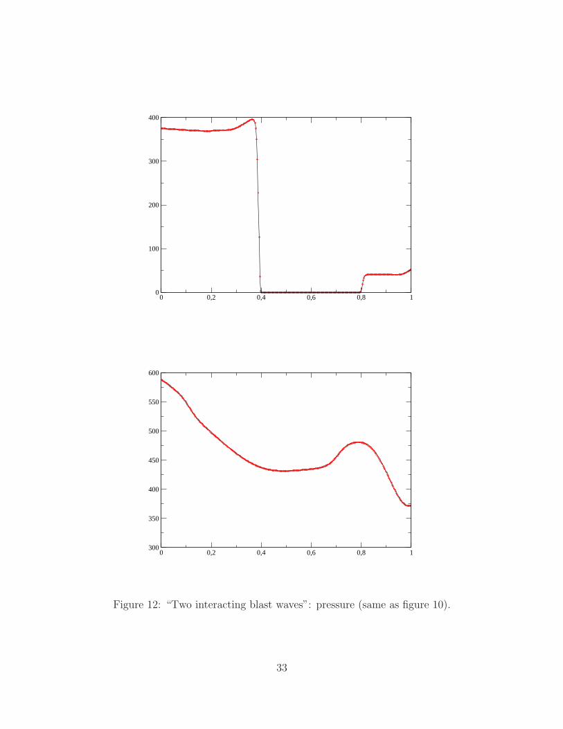
Here, the bounds of the global grid of the DVM are determined by the largest initialtemperature (we get ±126.5), and its step size is given by the smallest initial temperature.Then we find that the coarsest global grid that satisfies conditions (5)-(6) has not less than2 551 velocities! In figures 10–12, we observe that the LDV method requires only 30 velocitiesto give results that are very close to the DVM method (with 2 551 velocities), both beforeand after the shock. This proves the high efficiency of the LDV approach for this case. Notethat here again, we use a 4 point ENO interpolation in the LDV method.
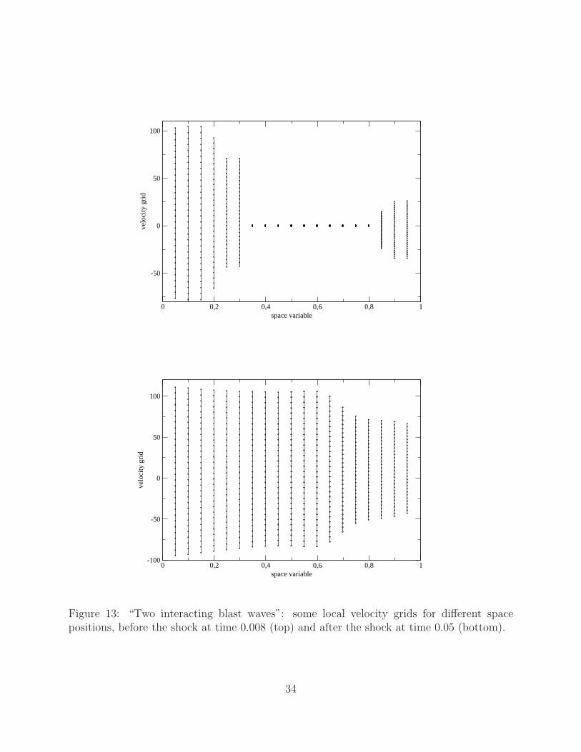
Finally, we plot in figure 13 some local velocity grids for different space positions: inthese plots, each vertical line is a local velocity grid, and its nodes are the small dots on theline. Note that before the waves interaction (top), the velocity grids in the middle of the
15
domain are much smaller than the grid in the left state, which is due to the different order ofmagnitude of the temperature at this time. After the interaction, the temperature is morehomogeneous, and the grids as well (see the bottom plot in this figure).
4.3 Heat transfer problem
In this test, we consider the evolution of a gas enclosed between two walls kept at temperatureTL = 300 and TR = 1000. At these walls, the distribution function satisfies the diffuseboundary condition
f(x = 0, v > 0) = MρL,0,TL, f(x = 1, v < 0) = MρR,0,TR
(25)
where
ρL = −∫
v<0vf(x = 0, v)dv
∫
v>0vM1,0,TL
dv, ρR = −
∫
v>0vf(x = 1, v)dv
∫
v<0vM1,0,TR
dv, (26)
and Mρ,0,T denotes ρ/√2πRT exp(−v2/2RT ) for every ρ and T . The initial data is the
Maxwellian with density ρ0 (to be defined later), velocity u0 = 0, and T0 = 300. Here, therelaxation time is defined with ω = −0.5 and c = 6.15 · 10−9.
The boundary conditions are taken into account in our numerical scheme by a ghost celltechnique, as it is standard in finite volume schemes. Left and right ghost cells are definedfor i = 0 and i = imax +1, and the velocity grids Vn
0 and Vnimax+1 in these cells are defined so
as to correctly describe the corresponding wall Maxwellians. Then, the density ρL and ρR,that are defined as the ratio of an outgoing mass flux at a wall to the corresponding incomingMaxwellian mass flux, are approximated by using the boundary cell and the correspondingghost cell, that is to say:
ρL = −〈v−fn
1 〉Vn
1
〈v+M(1, 0, TL)〉Vn
0
, ρR = −〈v+fn
imax〉Vn
imax
〈v−M(1, 0, TR)〉Vn
imax+1
.
For this test, we use the moment correction method with fourth order ENO interpolation,except for the computations discussed at the end of this section (see remark 4.1 below). Wealso use several Knudsen numbers Kn here. This number is parametrized by the initialdensity ρ0. We first analyze the LDV method in the transitional regime (ρ0 = 1.88862 10−5,which gives Kn = 10−2): here, both the LDV and DVM are converged with 30 velocities(the bounds of the global grid are ±1825.34), while the space domain [0, 1] is discretizedwith 1000 points. However, the results obtained with the LDV are not accurate enough (seefigure 14). An analysis of this problem shows that this is due to the local grid close to theright boundary which is not large enough: for small times, the distributions at these pointsare highly non symmetric.
To correct this problem, we use the algorithm proposed in section 3.4 to enlarge the localgrids in a non symmetric way. Then, the LDV with 30 velocities now gives results that areindistinguishable from the DVM, see figure 15.
16

Then, we test the LDV method in the rarefied regime (Kn = 1, ρ0 = 1.88862 10−7):the LDV (with enlarged non symmetric local grids) and the DVM are converged with 300velocities, while the space domain [0, 1] is discretized with 300 points. Here again, bothmethods give results that are almost indistinguishable (see figure 16). Unfortunately, thenumber of velocities required to get converged results is very large here, even for the LDV (300velocities). This is probably due to the fact that the distribution function is discontinuouswith respect to the velocity in this test, with very large jumps: our velocity grids, eventhe local ones, are uniform, and cannot capture these discontinuities when the number ofvelocities is too small. However, we show in figure 17 the results obtained with 50 velocitiesonly, and we observe that the LDV gives results that are more accurate than the DVM.
Finally, we did the same computations for Kn = 10 (ρ0 = 1.88862 10−8) and Kn = 1000(ρ0 = 1.88862 10−10) and we observed the following. First, the plateau phenomenon in theDVM approach with 100 velocities is clearly seen with Kn= 10 (while it was only slightlyvisible for Kn = 1). For Kn = 1000, the results are almost the same. For the LDV, whenthe number of discrete velocities is the same as for the DVM, the results are close to thereference solution (no plateau, no oscillations) for Kn = 10 and Kn = 1000, which is muchbetter than with the DVM (see figures 18 and 19). When the number of velocities is notlarge enough (30 points tested here), both method give wrong results, even if the LDV isbetter.
Remark 4.1. We also compare our LDV method with and without the moment correctionstep, for P1 and fourth order ENO interpolation. We do not find it usefull to add thecorresponding curves in this paper, but our observations are summarized below:
• for Kn = 0.01, there is not much difference if the moment correction method is usedor not:
– with fourth order ENO interpolation, both methods give good results, even if wenote a solution which is slightly less smooth without the moment correction step(there are a few small peaks).
– if the P1 interpolation is used, both methods give a wrong solution (with smalloscillations without the moment correction method).
• for larger Kn, (Kn = 1, 10, 1000):
– if the moment correction method is not used, we observe oscillations whose am-plitude increases with Kn, regardless of the interpolation.
– with the moment correction method and the P1 interpolation, the difference be-tween the numerical results and the reference solution increases with Kn, exceptif the number of discrete velocities is increased too.
4.4 CPU time comparisons
We have compared the CPU cost of our method (on a single processor Pentium(R) Dual-Core CPU E65002.9GHz) to the standard DVM with a global grid, by using the fortran
17

subroutine cpu time, and the following test cases:
• Sod test: we compared the DVM with 30 discrete velocities (shown in figures 4–6 (top)to our LDV with 30 points, 4 points ENO interpolation, and the moment correctionmethod (shown in figures 7–9);
• Blast waves: test case shown in figures 10–12 (bottom);
• Heat transfer: comparison between the LDV with 50 velocities and non symmetricgrids, to the DVM with 50 velocities (see figure 17).
We observed (see table 1) that our method with local velocity grids is more expensivethan the global grid method for Sod et heat transfer tests. Since the number of velocitiesin the grids is smaller with our method, this increase in CPU cost is probably due to thevery large number of interpolations made in the evaluation of reconstructed distributions.At the contrary, for the blast wave problem, the number of velocities is so large in the globalgrid that our method is less expensive. However, as expected, the gain factor in CPU time(which is 45) is smaller than the gain factor in number of velocities (which is 85).
We point out that the implementation of our method has not been optimized in thiswork, and such an optimization would probably make the method faster. However, thesecomparisons show that our algorithms have to be improved to be less computationally ex-pensive, in particular to reduce the cost of the reconstructions of the distribution in theirlocal grids. This is now investigated in a forthcoming work for 2D problems.
5 Conclusion and perspectives
We have presented a new velocity discretization of kinetic equations of rarefied gas dynamics:in this method, the distribution functions are discretized with velocity grids that are localin time and space, contrary to standard discrete velocity or discrete ordinate methods. Thelocal grids dynamically adapt to time and space variations of the support of the distributionfunction, by using the conservation laws.
This method is very efficient in case of strong variations of the temperature, for which astandard discrete velocity method requires a very large number of velocities. Moreover, itallows to eliminate the plateau phenomenon in very rarefied regimes.
We mention that in this study, the space discretization is a simple first order upwindmethod, which is known to have a very low accuracy. However, our method is quite in-dependent of the space approximation: any higher order finite volume or finite differenceapproximation could be used. For instance, a second order upwind scheme with limiters canbe used very easily by adding a flux limiter in (8) and slope limiters in (12). However, inthis preliminary work, we find it simpler to use a first order scheme to analyze the propertiesof the method, and to compare its advantages and drawbacks. We defer the investigationof higher order schemes to a work in progress in which our method will be extended tomulti-dimensional problems and its computational cost will be reduced.
18

Moreover, several aspects of the method should be better understood, in particular, whyare there some oscillations if the moment correction method is not used, in the rarefied andfree transport regimes, even with high order ENO interpolation? A mathematical analysisof the numerical method could be interesting here.
Acknowledgements. This study has been carried out in the frame of “the Investmentsfor the future” Programme IdEx Bordeaux – CPU (ANR-10-IDEX-03-02).
References
[1] V.V. Aristov. Method of adaptative meshes in velocity space for the intense shock waveproblem. USSR J. Comput. Math. Math. Phys., 17(4):261–267, 1977.
[2] C. Baranger, J. Claudel, N. Herouard, and L. Mieussens. Locally refined discrete ve-locity grids for deterministic rarefied flow simulations. AIP Conference Proceedings,1501(1):389–396, 2012.
[3] C. Baranger, J. Claudel, N. Herouard, and L. Mieussens. Locally refined discrete velocitygrids for stationary rarefied flow simulations. Journal of Computational Physics, 257,Part A(0):572 – 593, 2014.
[4] Mounir Bennoune, Mohammed Lemou, and Luc Mieussens. Uniformly stable numericalschemes for the boltzmann equation preserving the compressible navier–stokes asymp-totics. Journal of Computational Physics, 227(8):3781 – 3803, 2008.
[5] G.A. Bird. Molecular Gas Dynamics and the Direct Simulation of Gas Flows. OxfordScience Publications, 1994.
[6] A. V. Bobylev and S. Rjasanow. Fast deterministic method of solving the Boltzmannequation for hard spheres. Eur. J. Mech. B Fluids, 18(5):869–887, 1999.
[7] A.V. Bobylev, A. Palczewski, and J. Schneider. A Consistency Result for a Discrete-Velocity Model of the Boltzmann Equation. Siam J. Numer. Anal., 34(5):1865–1883,1997.
[8] C. Buet. A Discrete-Velocity Scheme for the Boltzmann Operator of Rarefied GasDynamics. Transp. Th. Stat. Phys., 25(1):33–60, 1996.
[9] S. Chen, K. Xu, C. Lee, and Q. Cai. A unified gas kinetic scheme with moving meshand velocity space adaptation. Journal of Computational Physics, 231(20):6643 – 6664,2012.
[10] Pierre Degond, Giacomo Dimarco, and Lorenzo Pareschi. The moment-guided MonteCarlo method. Internat. J. Numer. Methods Fluids, 67(2):189–213, 2011.
19

[11] G. Dimarco and L. Pareschi. Asymptotic preserving implicit-explicit Runge-Kutta meth-ods for nonlinear kinetic equations. SIAM J. Numer. Anal., 51(2):1064–1087, 2013.
[12] F. Filbet and T. Rey. A Rescaling Velocity Method for Dissipative Kinetic Equations -Applications to Granular Media. 27 pages, 2012.
[13] U. Fjordholm, S. Mishra, and E. Tadmor. Eno reconstruction and eno interpolation arestable. Foundations of Computational Mathematics, 13:139–159, 2013.
[14] J.R.Haack and I.M. Gamba. Conservative deterministic spectral boltzmann solver nearthe grazing collisions limit. AIP Conference Proceedings, 2012.
[15] V.I. Kolobov and R.R. Arslanbekov. Towards adaptive kinetic-fluid simulations ofweakly ionized plasmas. Journal of Computational Physics, 231(3):839 – 869, 2012.
[16] V.I. Kolobov, R.R. Arslanbekov, V.V. Aristov, A.A. Frolova, and S.A. Zabelok. Unifiedsolver for rarefied and continuum flows with adaptive mesh and algorithm refinement.Journal of Computational Physics, 223(2):589 – 608, 2007.
[17] V.I. Kolobov, R.R. Arslanbekov, and A.A. Frolova. Boltzmann solver with adaptivemesh in velocity space. In 27th International Symposium on Rarefied Gas Dynamics,volume 133 of AIP Conf. Proc., pages 928–933. AIP, 2011.
[18] L. Mieussens. Discrete Velocity Model and Implicit Scheme for the BGK Equation ofRarefied Gas Dynamics. Math. Models and Meth. in Appl. Sci., 8(10):1121–1149, 2000.
[19] L. Mieussens. Discrete-velocity models and numerical schemes for the Boltzmann-BGKequation in plane and axisymmetric geometries. J. Comput. Phys., 162:429–466, 2000.
[20] V.A. Panferov and A. G. Heintz. A new consistent discrete-velocity model for theboltzmann equation. Mathematical Methods in the Applied Sciences, 25(7):571–593,2002.
[21] Sandra Pieraccini and Gabriella Puppo. Implicit–explicit schemes for bgk kinetic equa-tions. Journal of Scientific Computing, 32:1–28, 2007.
[22] P.Woodward and P.Colella. The numerical simulation of two-dimensional fluid flow withstrong shocks. J. Comput. Phys., 54:115–173, 1984.
[23] F. Rogier and J. Schneider. A Direct Method For Solving the Boltzmann Equation.Transp. Th. Stat. Phys., 23(1-3):313–338, 1994.
[24] C.-W. Shu. Essentially non-oscillatory and weighted essentially non-oscillatory schemesfor hyperbolic conservation laws. Technical Report 97-65, ICASE, 1997.
[25] S. Takata, Y. Sone, and K. Aoki. Numerical analysis of a uniform flow of a rarefied gaspast a sphere on the basis of the boltzmann equation for hard-sphere molecules. Physicsof Fluids A: Fluid Dynamics, 5(3):716–737, 1993.
20

[26] V. A. Titarev. Efficient deterministic modelling of three-dimensional rarefied gas flows.Communications in Computational Physics, 12(1):162–192, 2012.
[27] K. Xu and J.-C. Huang. A unified gas-kinetic scheme for continuum and rarefied flows.J. Comput. Phys., 229:7747–7764, 2010.
21

Figure 1: Three distribution functions in different space points of a computational domainfor a re-entry problem, and the corresponding global discrete velocity grid V .
22

0 0,1 0,2 0,3 0,4 0,50,002
0,003
0,004
0,005
0,006
0,007
0,008
0 0,1 0,2 0,3 0,4 0,50
0,1
0,2
0,3
0,4
0,5
0,6
Figure 2: Sod test case, rarefied regime: temperature (top) and velocity (bottom) profiles,at time 7.34 10−2. The solid line is the reference solution obtained with the DVM with theenlarged global grid (600 points), the dotted line is the DVM with an incorrect grid (100points), while the dot-dashed line is the LDV method (30 points).
23

0 0,1 0,2 0,3 0,4 0,50,002
0,003
0,004
0,005
0,006
0,007
0,008
0 0,1 0,2 0,3 0,4 0,50
0,1
0,2
0,3
0,4
0,5
0,6
Figure 3: Sod test case, fluid regime: temperature (top) and velocity (bottom) profiles, attime 7.34 10−2. The solid line is the reference solution obtained with the DVM with theenlarged global grid (100 points), the dotted line is the DVM with an incorrect grid (100points), while the dot-dashed line is the LDV method (10 points).
24

-1 -0,5 0 0,5 1
0,6
0,8
1
1,2
1,4
1,6
1,8
2
2,2
2,4
-1 -0,5 0 0,5 10
0,5
1
1,5
2
2,5
3
Figure 4: Sod test case, free transport: temperature at time 0.3. Top: comparison betweenthe exact solution (dot-dashed) and with a 30 points DVM (solid). Bottom, comparisonbetween the exact solution (dot-dashed) and several LDVs with 30 points: with first orderinterpolation (’o’), with 3 points-ENO (dotted), with 4 points-ENO (solid).
25

-1 -0,5 0 0,5 10
0,2
0,4
0,6
0,8
-1 -0,5 0 0,5 10
0,2
0,4
0,6
0,8
Figure 5: Same as figure 4 for the velocity.
26

-1 -0,5 0 0,5 10
0,2
0,4
0,6
0,8
1
-1 -0,5 0 0,5 10
0,2
0,4
0,6
0,8
1
Figure 6: Same as figure 4 for the density.
27

-1 -0,5 0 0,5 1
0,6
0,8
1
1,2
1,4
1,6
1,8
2
Figure 7: Sod test case, free transport: temperature at time 0.3, comparison between theexact solution (dot-dashed) and several LDVs with 30 points and the moment correctionmethod: with first order interpolation (’o’), with 3 points-ENO (dotted), with 4 points-ENO(solid).
28

-1 -0,5 0 0,5 10
0,2
0,4
0,6
0,8
1
Figure 8: Sod test case, free transport: velocity at time 0.3, comparison between the exactsolution (dot-dashed) and several LDVs with 30 points and the moment correction method:with first order interpolation (’o’), with 3 points-ENO (dotted), with 4 points-ENO (solid).
29

-1 -0,5 0 0,5 10
0,2
0,4
0,6
0,8
1
Figure 9: Sod test case, free transport: density at time 0.3, comparison between the exactsolution (dot-dashed) and several LDVs with 30 points and the moment correction method:with first order interpolation (’o’), with 3 points-ENO (dotted), with 4 points-ENO (solid).
30

0 0,2 0,4 0,6 0,8 10
0,5
1
1,5
2
2,5
3
0 0,2 0,4 0,6 0,8 10
1
2
3
4
Figure 10: “Two interacting blast waves”: temperature, before the shock at time 0.008 (top)and after the shock at time 0.05 (bottom). The solid line is the solution obtained with theLDV method (30 points), the dotted line is the solution computed with the DVM method(2 551 velocities).
31

0 0,2 0,4 0,6 0,8 1-5
0
5
10
15
20
0 0,2 0,4 0,6 0,8 1
8
10
12
14
16
18
20
Figure 11: “Two interacting blast waves”: velocity (same as figure 10).
32
0 0,2 0,4 0,6 0,8 10
100
200
300
400
0 0,2 0,4 0,6 0,8 1300
350
400
450
500
550
600
Figure 12: “Two interacting blast waves”: pressure (same as figure 10).
33
0 0,2 0,4 0,6 0,8 1space variable
-50
0
50
100
velo
city
gri
d
0 0,2 0,4 0,6 0,8 1space variable
-100
-50
0
50
100
velo
city
gri
d
Figure 13: “Two interacting blast waves”: some local velocity grids for different spacepositions, before the shock at time 0.008 (top) and after the shock at time 0.05 (bottom).
34

0 0,1 0,2 0,3 0,4 0,5300
400
500
600
700
800
900
1000
0 0,1 0,2 0,3 0,4 0,5-50
-40
-30
-20
-10
0
Figure 14: Heat transfer problem, transitional regime: temperature (top) and velocity (bot-tom) at time 1.3 10−3, Kn = 10−2. The solid line is the solution given by the LDV method(30 velocities), the dot-dashed line is the DVM method (30 velocities).
35

0 0,1 0,2 0,3 0,4 0,5 0,6300
400
500
600
700
800
900
0 0,1 0,2 0,3 0,4 0,5 0,6-50
-40
-30
-20
-10
0
Figure 15: Heat transfer problem, transitional regime (test of the non symmetric local grid):temperature (top) and velocity (bottom) at time 1.3 10−3, Kn = 10−2. The solid line is thesolution given by the LDV method (30 velocities), the dot-dashed line is the DVM method(30 velocities).
36

0 0,1 0,2 0,3 0,4 0,5 0,6400
450
500
550
600
650
700
0 0,1 0,2 0,3 0,4 0,5 0,6-30
-25
-20
-15
-10
-5
0
Figure 16: Heat transfer problem, rarefied regime: temperature (top) and velocity (bot-tom) at time 1.3 10−3, Kn = 1. The solid line is the solution given by the LDV method(300 velocities, non symmetric local grids), the dot-dashed line is the DVM method (300velocities).
37

0 0,1 0,2 0,3 0,4 0,5 0,6400
450
500
550
600
650
700
0 0,1 0,2 0,3 0,4 0,5 0,6-30
-25
-20
-15
-10
-5
0
Figure 17: Heat transfer problem, rarefied regime: temperature (top) and velocity (bottom)at time 1.3 10−3, Kn = 1. The solid line is the solution given by the LDV method (50velocities, non symmetric local grids), the dot-dashed line is the DVM method (50 velocities),the dashed line is the DVM method with 300 velocities (reference solution).
38

0 0,1 0,2 0,3 0,4 0,5 0,6
450
500
550
0 0,1 0,2 0,3 0,4 0,5 0,6-20
-15
-10
-5
0
Figure 18: Heat transfer problem, rarefied regime: temperature (top) and velocity (bottom)at time 1.3 10−3, Kn = 10. The solid line is the LDV method with 100 velocities, the dot-dashed line is the DVM method (100 velocities), the dashed line is the solution given by theDVM method (400 velocities, reference solution).
39

0 0,1 0,2 0,3 0,4 0,5 0,6420
440
460
480
500
520
540
0 0,1 0,2 0,3 0,4 0,5 0,6-20
-15
-10
-5
0
Figure 19: Heat transfer problem, rarefied regime: temperature (top) and velocity (bottom)at time 1.3 10−3, Kn = 1000. The solid line is the LDV method with 100 velocities, thedot-dashed line is the DVM method (100 velocities), the dashed line is the solution given bythe DVM method (400 velocities, reference solution).
40

Sod Blast waves Heat transferDVM 0.344 949 64LDV 5.136 20 14
Table 1: CPU time comparisons (in seconds) between the LDV and DVM methods
41