Manual version: 2.0

Local Climate Zones Classification

Introduction

The purpose of this practical is to provide instructions on how to how to generate local climate zones (Stewart and

Oke, 2012) for an urban area using remote sensing images and software (Bechtel and Daneke, 2012). This practical

is based on the process developed by Benjamin Bechtel and the examples are drawn from work completed by Paul

Alexander and Mícháel Foley. It is separated into two parts, each of which employs freely sourced software.

Part 1 Google Earth (GE) tools are used to establish the urban domain under study (known as the region

of interest, ROI) and to define areas within the domain that typify LCZ types.

Part 2 Satellite data (e.g. Landsat 8) are acquired and processed with the SAGA system, an open source

remote sensing and GIS system. The entire ROI is classified into LCZ types using the training areas

provided in Part 1.

Software Required: Google Earth: www.google.com/earth/download/ge/agree.html

SAGA GIS: http://sourceforge.net/projects/saga-gis/files/

You will also need to obtain the file LCZ Template.kmz, which is a generic set of labels that are used store

information on each LCZ type and is available in the group dropbox folder.

WUDAPT Manual

1

Part 1: Google Earth Google Earth (GE) software is an essential part of this Exercise as it provides global coverage, high quality satellite

data that is geocoded and has tools for mapping, measuring and digitizing. Here we use GE to create the working

domain (a region of interest), which is a rectangular area that contains the urban area of interest. We also use GE

to delineate individual LCZ areas that will be used subsequently as training areas when classifying Landsat images.

The files used by GE use Keyhole Markup Language, which have a kmz extension when compressed; here we

generate kmz file that contains the geographic information we will use in Part 2.

1.1 Region of interest (ROI): 1. Open GE and open the file LCZ Template.kmz, which you should store in a work folder (here we name this

folder LCZ). Note that on the left hand window under MyPlaces, each of the LCZ types are listed in folders.

LCZ types 1-10 represent the urban landscape (LCZ1 – LCZ 10) and 101-107 represents LCZ A to LCZ G,

2. Use GE tools (search, pan, etc.) to relocate the window over the city under study. Zoom in/out using the

ruler on the right hand side until the urban area is centered.

3. Create the ROI by drawing an area (known as a polygon) around the urban area. Click the “Add polygon”

tool along the top bar. Once the “New Polygon” window appears, simply name the polygon ROI. A cross-

hair (+) appears on the screen that moves with the movements of the mouse. Each time you left-click, a

marker is placed on the map; each subsequent marker is attached to the previous marker by a straight

line. Place markers on the image so that the ROI polygon is created.

Fig 1. Showing key points to be observed when creating ROI polygon.

2. Add polygon.

1. Making sure the template

is highlighted.

WUDAPT Manual

2

When selecting the ROI:

It should be large enough to contain the entire urban area you wish to analyze but not so large so that unnecessary analysis is needed.

It should have a simple square/rectangular shape.

Think of size of ROI as entire urban agglomeration including a significant portion of the surrounding

natural or rural area.

In Fig. 2 below the ROI for Dublin is shown; it includes large areas that are either water or non-urban but it is

ideally sized to capture the variety of LCZ (both urban and natural) in the study area.

l

Fig 2. An example of an ROI polygon around Dublin city.

1.2 Training areas: Training areas created within the LCZ Template.kmz are used to analyze and classify the remote sensing images

used in Part 2 of this exercise. These areas are small portions of the ROI where the landscape that typifies a LCZ is

found; this is where your knowledge of the city is most important. Choose the LCZ you wish to sample and search

WUDAPT Manual

3

the city under study to find a suitable area that corresponds to that type. The area should be ≥1km2 and more

than 150 m wide at its narrowest.

To illustrate here we will delineate an example of an open set low-rise neighborhood (LCZ 6) from within Dublin.

Once a suitable training area has been found, right click on the corresponding folder within the template and choose

to add a new polygon, as shown in Fig. 3. Once the “New Polygon” window will appears, simply name the polygon

after the LCZ you are sampling and continue to digitize.

Fig 3. Showing how to add a polygon in relation to a training area.

Fig 4. An example of a training area polygon in Dublin city.

In Fig. 4 the training area has identified a suburban area that is well vegetated. Once the training area has been

completed, change the style setting for that LCZ type; right-click on the accompanying LCZ folder and select

Properties >Style, Color>Share Style. Repeat the digitizing process for the same LCZ type so that we have a

number of examples to use for training.

Now select another LCZ and repeat the same process as above.

WUDAPT Manual

4

Fig 5. Varying examples of how to sample training areas.

Fig. 5 shows varying examples of how to capture training areas. Remember, that the classification using Landsat

images will be conducted for a grid with cells 100-200 m on the side, so look for larger homogenous areas and ignore

patches smaller than this size. The geometric accuracy of the training area boundaries is not critical since the

classification is completed for a relatively coarse grid. Hence, it might be appropriate to leave a buffer of about 100

m to the next LCZ, if there is a clear boundary. Take into account the optimal size and shape of training areas (> 1

km2 and >150m wide at the narrowest point) and try to make the training area as uniform in shape as possible.

Ideally there should be several examples (5-15) of each LCZ to help in the automatic classification; there will be

variations between a LCZ type in different parts of the city (e.g. different roof colors or building materials) and in the

same LCZ at different times of the year owing to vegetation status) so make sure to digitize examples.

If possible, digitize features that are fairly persistent in time (years), no construction sites, harvested fields, etc.

When complete you will have digitized several polygons: the ROI that includes the entire area under study and

several smaller polygons that outline areas of different LCZ types within the ROI.

Once digitizing is complete, rename the LCZ Template file to reflect the city under study and the date. In the example

above it is renamed Dublin_31012014, that is the Dublin files created on the 31st January, 2014.

Finally, save this file as a kml file (this is not the default). This file contains the geographic co-ordinates of the

boundary that outlines each of the polygons digitized (this is a vector file).

A video showing this process is available on the WUDAPT website.

WUDAPT Manual

5

Part 2: System for Automated Geoscientific Analyses (SAGA)

SAGA is freely available software that has a number of Geographic

Information System and Image Analysis tools. It is available at:

http://www.saga-gis.org/en/index.html. On this site you will find

documentation, including the manual. In this exercise we use Landsat 8 (L8)

products to show how the training areas can be used within SAGA to classify

the ROI into LCZ types. L8 data is freely available, has a global coverage and

is multispectral (see attached document for the electromagnetic bands and

spatial resolution).

In this part of the exercise, we use the vector kml file produced in Part 1 to clip a section of a satellite image for

further analysis using the ROI. We then use the training areas to guide the classification of the entire ROI into LCZ

types. You will see that each operation in GIS results in the creation of a new file; as we will complete several

operations the result will be a large number of files. Good file management, which includes deleting those files no

longer needed, is essential when using SAGA. The sequence followed here is:

1. Import: this brings both the satellite image (raster) and the kml (vector) files into SAGA

2. Merge: The information in the training areas is merged.

3. Project: Transform the co-ordinate system of the kml files to match the raster image.

4. Clip: The ROI is used to ‘clip’ the satellite image so that only the area of interest is available for classification.

5. Resample: Bring the dataset to the optimal resolution of LCZ classification.

6. Classify: After pre-processing an algorithm (random forest) classifies cells into LCZ types using the training

areas as a guide.

7. Filter: After the classification, a filtering routine is used to remove individual cells and clusters too small to

form a neighbourhood (LCZ) scale.

8. Export to GE for evaluation. The LCZ map is exported to GE so that the classification can be evaluated using

GE.

An overview of the procedure is given in Fig 6.

WUDAPT Manual

6

workflow

Digitize

training data

Load LS dataGDAL: Import

Raster

Supervised

classificationRandom Forest

(ViGra)

Google Earth SAGA

Resample

1. grid systemResampling

Crop to ROIClip Grid with

Polygon

Load KMLOGR: Import

Vector Data

MergeMerge

Layers

Resample

further grid systResampling

EavaluateExport 2 KMLExport Grid to KML

Post class

filteringMajority Filter

ProjectCoordinate

transformation

(shapes)

Remember

documentation !!!

Fig 6: Workflow of the LCZ classification in SAGA

2.1 Import:

2.1.1 Import satellite Imagery

Geoprocessing > File > GDAL/OGR > GDAL: Import Raster

Once the import raster data window opens, select the required satellite images. Deselect the “Transformation”

option.

Fig 7. An image showing the pathway to the “import Raster” option. Look inside your city folder on the desktop

WUDAPT Manual

7

2.1.2 Import KML Files Geoprocessing > File > GDAL/OGR > ORG: Import Vector Data

Once the “import vector data” window opens, select the ROI file created during Part 1. When importing KML files

change the option “Geometry Type” from “automatic” to “wkbPolygon”. Repeat with training area file.

Fig 8. An image showing the pathway to the “import vector data” option.

You will see the entire set of LCZ polygons in the kml file appear in the left window, even though some are empty.

2. 2 Merge The training areas are merged to create a single LCZ file

Geoprocessing > Shapes > Construction > Merge Layers

Now that our training areas are imported, we will merge the information that they contain. In the “Merge Layers”

window, select all the LCZ training areas (not the ROI). Make sure that the options, “Add Source information” and

“Match Files by Name” are both selected. Once the layers have been merged a new polygon named “Merged

Layers” will appear in the list of polygons in the left-hand window. You can remove the old LCZ files and save the

new merged file.

Fig 9. An image showing the Merge Layers window.

WUDAPT Manual

8

2.3 Project Geoprocessing > Projection > Coordinate Transformation (Shapes list)

Once the “Coordinate Transformation (Shapes list)” window opens, select the “Loaded Grid” option. A separate

window will then open:

1. Select one Grid that will be used as the co-ordinate system to geo-reference the KML vector file

2. Open the “Source” option and select the KML files you wish to geo-reference.

Fig 10. An image showing the Coordinate Transformation (Shapes list) window.

To check your results, open the satellite image used as the geo-reference file and the KML files. If the coordinate

system has transferred correctly to the KML the ROI and the training areas should overlay correctly, as seen below.

Fig 11. An image showing how the ROI and training areas should overlay after been georeferenced.

WUDAPT Manual

9

2.4 Clip The satellite image is clipped to the size of the ROI:

Geoprocessing > Shapes > Girds > Spatial Extent > Clip Grid with Polygon

Select the grids that you want to ‘clip’; the polygon that will be used to do this is the ROI polygon imported above

(see Fig. 12)

Fig 12. An image showing the Clip Grid with Polygon window.

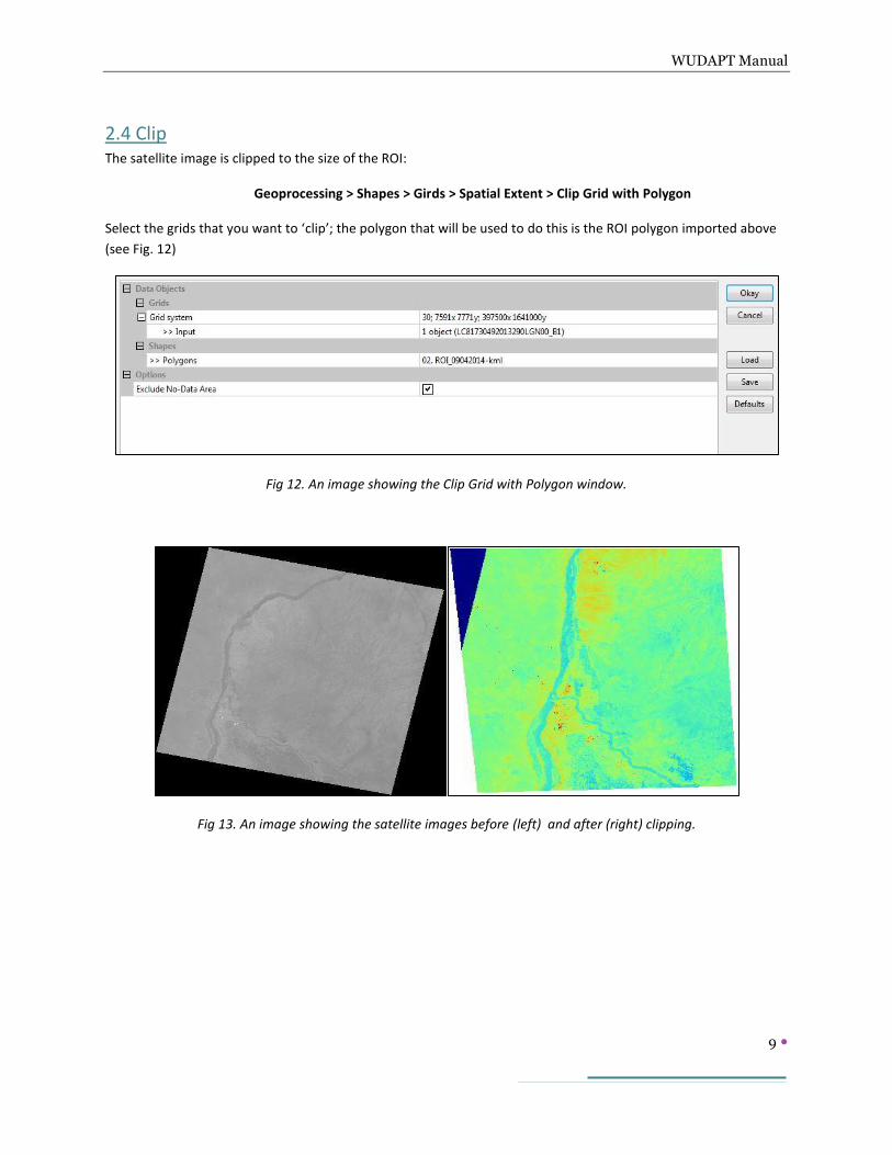
Fig 13. An image showing the satellite images before (left) and after (right) clipping.

WUDAPT Manual

10

2.5 Resample Landsat8 scenes consist of 12 bands (B1 to B12), which have different spatial resolutions: B8 (panchromatic) is 15

m; B11 & B12 (thermal) are 100 m and; the remainder are 30 m. To integrate the information contained, we need

to resample these bands to the same grid. Here we resample our Landsat scene to a grid of 120 m resolution.

However, you can try if slightly different resolutions (90 m, 100 m, 150 m) give better results.

Geoprocessing > Grids > Grid Systems > Resampling

Once the first “Resampling” window has opened, select the B1 as the first grid to be resampled. Add all the other bands

in the “Additional Grids” box. In the additional options, make sure to select “Preserve Data Type” and to set “Target

Grid” to user defined.

Fig 14. An image showing the Merge Layers window first Resampling window.

Once the previous step is complete, a new window will open and you select create; this will generate new grids for

all the bands being resampled. Specify a cell size of 120 m.

Fig 15. An image showing the Merge Layers window second Resampling window.

Finally, you will be asked to select an interpolation method, that is, how is the 30 m data to be translated to the

120 m grid? Here we select the option “Mean Value (cell area weighted)”.

WUDAPT Manual

11

Fig 16. An image showing the Merge Layers window second Resampling window.

At this point the computer will take some time to process the Landsat scene and each of the bands. On the left

hand side you will see that it generates a set of grid files that ‘mirror’ the original band information. It is the

resampled grid bands that we will be using so you can remove the original grids. At this point it is worth saving

your files.

2.6 Classify This process classifies the Landsat image using the training areas.

Geoprocessing > Imagery > Classification > Random Forest (ViGrA)

Once the “Random Forest (ViGrA)” window opens, first select the prepared satellite images which wish to classify,

Making sure that the two additional options “Random Forest Classification” and “Prediction Probability” are both

set to create.

Next, when asked for “Training Areas” select the Merged Layers polygon which was created earlier. Make sure that

the “Label Filed” option is set to source and that the “Use Label as Identifier” option is selected.

Depending on the computer you are using, the classification may take a few minutes to be completed. Simply wait

and allow the program to run as normal.

WUDAPT Manual

12

Fig 16. An image showing the Random Forest (ViGrA) window.

Once the classification is complete, a new raster image called “Random Forest Classification” will appear in the list

of grids. This new image should somewhat resemble the image shown below.

Fig 17. An image showing a Random Forest Classification for Khartoum.

WUDAPT Manual

13

2.7 Filter The pixel based automatic classifier is likely to produce a ‘noisy’ outcome, with many pixels that exhibit isolated

LCZ values. To remove single pixels of one LCZ a post classification filter can be used. You can test the majority

filter with different neighborhoods:

Geoprocessing > Grid > Filter > Majority Filter

Fig 18 .Filter options.

Fig 19. Result of majority filtering with different radii for Houston. UL: Original classification, LL: r=1 px, UR: 2px, LR:

4 px. How “patchy” do you want your LCZ classification?

We recommend a post classification majority filter with 200-300 m radius.

WUDAPT Manual

14

2.8 Export to Google Earth

Geoprocessing > File > Grid > Export > Export Grid to KML

Make sure the filename includes basic information (which classifier, options, used features, filter) or you document

them somewhere else. Set coloring to “same as in graphical user interface”. Make sure you have chosen the

appropriate lookup table before (provided in materials). Chose PNG file format. Remove the interpolation tick. The

image is automatically projected.

Note that Google Earth can only display lat/lon images. For higher latitude this means distortion or loss of accuracy.

To display the raster in Google Earth in the best quality, it should be re-projected manually increasing the cell size

by factor 3-5 and then exported to KML. However, for a quick look the automated export is sufficient.

Fig 20 .Options of KML export.

Then a KML and a PNG image file will be generated. You can open the KML in Google Earth and evaluate the

classification visually. Set the transparency of the image overlay (contained in folder “Raster exported from SAGA”)

to approx. 50 %.

WUDAPT Manual

15

Fig 21 .Exported classification in Google Earth, Options of image overlay.

Evaluation The approach to LCZ generation here is iterative. The urban expert must examine the results to see whether the

process has generated an acceptable LCZ classification for the ROI. If not, then there are a couple of options:

1. Revisit the training areas and try to improve these by adding others – this will provide more guidance to

the automatic classification or;

2. Acquire more satellite data at greater spatial or spectral resolution.

Keep in mind that the Landsat 8 data used here represents just one image and reflects time of day and day of year;

in other words it is taken under specific weather and climate conditions that will affect the surface signals. One of

the biggest changes over the course of a year may be driven by changing vegetative growth (driven by solar energy

and water availability). Obtaining five clear-sky L8 images from across the seasons should be sufficient to capture

these variations. Of course, there is also the option of getting other satellite data at finer spatial resolution that

may help in the LCZ classification. Other sources of data such as land-use/land-cover data may also help in your

decision making.

WUDAPT Manual

16

Appendix: LANDSAT 8

Landsat 8 launched on February 11, 2013, from Vandenberg Air Force Base, California, on an Atlas-V 401 rocket, with

the extended payload fairing (EPF) from United Launch Alliance, LLC. The Landsat 8 satellite payload consists of two science instruments—the Operational Land Imager (OLI) and the Thermal Infrared Sensor (TIRS). These two sensors provide seasonal coverage of the global landmass at a spatial resolution of 30 meters (visible, NIR, SWIR); 100 meters (thermal); and 15 meters (panchromatic).

Landsat 8 was developed as a collaboration between NASA and the U.S. Geological Survey (USGS). NASA led the design, construction, launch, and on-orbit calibration phases, during which time the satellite was called the Landsat Data Continuity Mission (LDCM). On May 30, 2013, USGS took over routine operations and the satellite became Landsat 8. USGS leads post-launch calibration activities, satellite operations, data product generation, and data archiving at the Earth Resources Observation and Science (EROS) center.

Evolutionary Advances: Landsat 8 instruments represent an evolutionary advance in technology. OLI improves on past Landsat sensors using a technical approach demonstrated by a sensor flown on NASA’s experimental EO-1 satellite. OLI is a push-broom sensor with a four-mirror telescope and 12-bit quantization. OLI collects data for visible, near infrared, and short wave infrared spectral bands as well as a panchromatic band. It has a five-year design life. The graphic below compares the OLI spectral bands to Landsat 7′s ETM+ bands. OLI provides two new spectral bands, one tailored especially for detecting cirrus clouds and the other for coastal zone observations.

The

OLI collects data for two new bands, a coastal band (band 1) and a cirrus band (band 9), as well as the heritage

Landsat multispectral bands. Additionally, the bandwidth has been refined for six of the heritage bands. The

Thermal Instrument (TIRS) carries two additional thermal infrared bands. Note: atmospheric transmission

values for this graphic were calculated using MODTRAN for a summertime mid -latitude hazy

atmosphere (circa 5 km visibility). Graphic created by L.Rocchio & J.Barsi.

WUDAPT Manual

17

Table courtesy of B. Markham (July 2013)

TIRS collects data for two more narrow spectral bands in the thermal region formerly covered by one wide spectral band on Landsats 4–7. The 100 m TIRS data will be registered to the OLI data to create radiometrically, geometrically, and terrain-corrected 12-bit data products.

Landsat 8 is required to return 400 scenes per day to the USGS data archive (150 more than Landsat 7 is required to capture). Landsat 8 has been regularly acquiring 550 scenes per day (and Landsat 7 is acquiring 438 scenes per day). This increases the probability of capturing cloud-free scenes for the global landmass. The Landsat 8 scene size is 185-km-cross-track-by-180-km-along-track. The nominal spacecraft altitude is 705 km. Cartographic accuracy of 12 m or better (including compensation for terrain effects) is required of Landsat 8 data products.

Source: http://landsat.gsfc.nasa.gov/?p=3186