Local bipartite turán graphs and graph partitioning

Local Bipartite Turhn Graphs and Graph Partitioning

Jon Lee*

Department of Mathematics, University of Kentucky, Lexington, Kentucky 40506-0027

Jennifer Ryan

Department of Mathematics, University of Colorado at Denver, Denver, Colorado 8021 7-3364

Motivated by the NP-hard problem of finding a minimum-weight balanced bipartition of an edge-weighted complete graph, we studied the class of graphs having the same degrees as bipartite Turim graphs. In particular, we established a maximal set of linear equations satisfied by the counts of the possible incidences of 3- and 4-cycles on such graphs. This leads to extremal results that we exploit in a heuristic for the partitioning problem, as well as in the computation of a Lagrangian bound. Preliminary computational results with the heuristic appear to be quite promising. Further results are established linking various adjacency concepts and measures of nonbipartiteness for such graphs. We also demonstrate the potential power of the Lagrangian bound via a family of examples. 0 1994 John Wiley & Sons, Inc.

1. INTRODUCTION

We assume some familiarity with graph theory (see, e.g., [ I ] ) . For an undirected graph F , let V ( F ) and E ( F ) denote the vertices and edges of F , respectively. We refer to K,,,/2,,rn/21 as a bipartiie Tirra‘n graph (or a BTG) on n vertices. One case of Turin’s Theorem ( I94 1 ), in fact, a case proved earlier by Mantel [ 171, implies that a simple graph on n vertices with 1 n / 2 JT n / 21 edges is triangle-free (i.e., K,-free) if and only if it is isomorphic to KLn/2,.rn,21

(see, e.g., [ 1, p. 2771). Let G be an arbitrary simple graph on n vertices with Ln/2 J vertices, denoted H ( G), ofdegree rn/21. and rn/21 vertices, denoted L ( G ) , of degree i n / 21. Any such graph G is referred to as a local bipartite Tzirbn graph (or an LBTG): note that Turiin’s Theorem implies that such an LBTG is bipartite if and only if it is

* Research conducted in part at CORE. Univenite Catholique de Louvain, Louvain-la-Neuve. Belgium, and supported in part by a CORE Fellowship and a Yale Senior Faculty Fellowship.

Supported by AFORS/ONR Contract #F49620-90-C-0033.

a BTG. When n is even, G is an n / 2 factor and the partition of V ( G) into H ( G) and L( G ) is arbitrary.

In Section 2 , we study the incidence of 3- and 4-cycles on an LBTG. In particular. we establish a maximal set of independent linear equations satisfied by the “counts” of the different possible incidences that 3- and 4-cycles can have with an LBTG. We also obtain extremal results that are used in the sequel. In Section 3 , we establish further results on the 3-cycle structure of LBTGs. In Section 4, we study the relationship between alternating exchanges (mostly 4-cycles) and measures of closeness (mostly the number of triangles) of an LBTG to the set of BTGs. In Section 5, we use some ofthese ideas to develop a heuristic for the NP-hard problem of finding a minimum-weight spanning BTG subgraph of an edge-weighted complete graph. Some computational results are provided. It is this partitioning problem that is the primary motivation for our work. In Section 6, we present a Lagrangian lower bound for this optimization problem and give a family of examples to illustrate its potential power as a computational tool. In addition, we demonstrate how the cal- culation of the bounded can be hastened, using a result

NETWORKS, VOl 24 (1994) 131-145 ’c 1994 John Wiley & Sons, Inc CCC 0028-3045/94/030131-15

131

132 LEE AND RYAN

f= Fig. 1.1. C,

from Section 2. Section 7 contains some brief remarks on possible extensions of our results. For the remainder of the present section, we set our notation and give some examples.

Throughout, G will denote an LBTG on n vertices. Let G denote the complement of G. SAT denotes the symmetric difference (S\ T ) U ( T\S) of sets S and T . For graphs G and G’ having V ( G ) = V ( G’), we denote by G 0 G’ (resp., GAG’), the graph having vertex set V ( G ) = V(G’ ) and edge set E ( G ) U E(G’) (E(G)AE(G’) ) . Let a be any vertex in L ( G ) [resp., H ( G ) ] , let N, = N,(G) denote the ~ n / 2 j (rn/21) neighbors of a (i.e., N J G ) = { b E V ( G ) : {a, b } E E ( G ) } ) , and let B, = B,( G ) denote the rn/21- 1 (Ln/2 J - 1 ) nonneighbors of a (i.e., B,(G) = (V(G)\N,)\ { a}). For a scalar X and an event S , As is defined to be X times the indicator function of the event S . Finally, for a vector x E %‘, neg( x) E 8’ is defined by neg( x ) ~ : = min { x i , 0 } for 1 - ( i i n .

We give another important example of an LBTG that will arise in the sequel. For S C V ( G ) , let E[S] be the set of edges with both endpoints in S, and let G [ S ] be the subgraph of G induced by S (i.e., V ( G [ S]) = S and E ( G [ S ] ) = E [ S ] ) . A closet graph on n vertices is any graph that is isomorphic to the graph C, = C,(W, W’), where I WI = tn/2j, I W‘I = Tn/21, V(C,) = W U W‘, C,,[ W ] and C,[ W’] are complete, and E(C,)\(E[ W ] U E [ W ‘ ] ) is an independent set of edges M of cardinality Ln/2 J (see [ 121). See Figure 1.1 for a drawing of C, . Closet graphs are LBTGs. If n is odd, then L( G ) is W together with the element of W’ that is not met by M .

It is possible to obtain many other LBTGs that are neither closet graphs nor BTGs by the following construction: Let G and G’ be two LBTGs on disjoint vertex sets. Taking the union of G and G’ together with all possible edges between L ( G ) and L(G’), and all possible edges between H ( G ) and H ( G’), yields another LBTG, called a cross product of G and GI. In the case that G or G‘ has an even number of vertices, there are many possible cross products. See Figure 2.4 for a cross product of C6 with K3,3, and of C, with K4,3.

Another way to build LBTGs is by balanced vertex expansion. Let G be an LBTG on 2k vertices. Define positive integers l,, for all o E V ( G ) , so that C 1, is con-

stant, over all o E V ( G ) . Define a new graph H having 1, vertices for each vertex o. Now for each edge (o, w) of

w € N ,

G , connect all 1, copies of o with all 1, copies of w. The resulting graph Hi s an LBTG on C 1, vertices. Figure

1.2 depicts a balanced vertex expansion of C6 with all 1, equal to 3.

u€V(G)

2. ON THE SMALL-CYCLE STRUCTURE

Let ,6 = p1P2 - - - be a binary string. We associate with each such binary string a set @( G, P ) of 1-cycles of edges of G 0 e = K,,. Consider an 1-cycle of edges C = (el , e2, . . . , el) from G 0 G. Define (? (G, P ) to be the set of such C such that there is a cyclic permutation ?r with

ei (,,,,, if r ( P ) i 2 1;

E ( G ) , if T ( P ) ~ = 0,

for all i . 1 I i I I. Now let

P(P> = P ( G , P ) = l@(G, P)I. Considering cyclic permutations T , and the equivalence

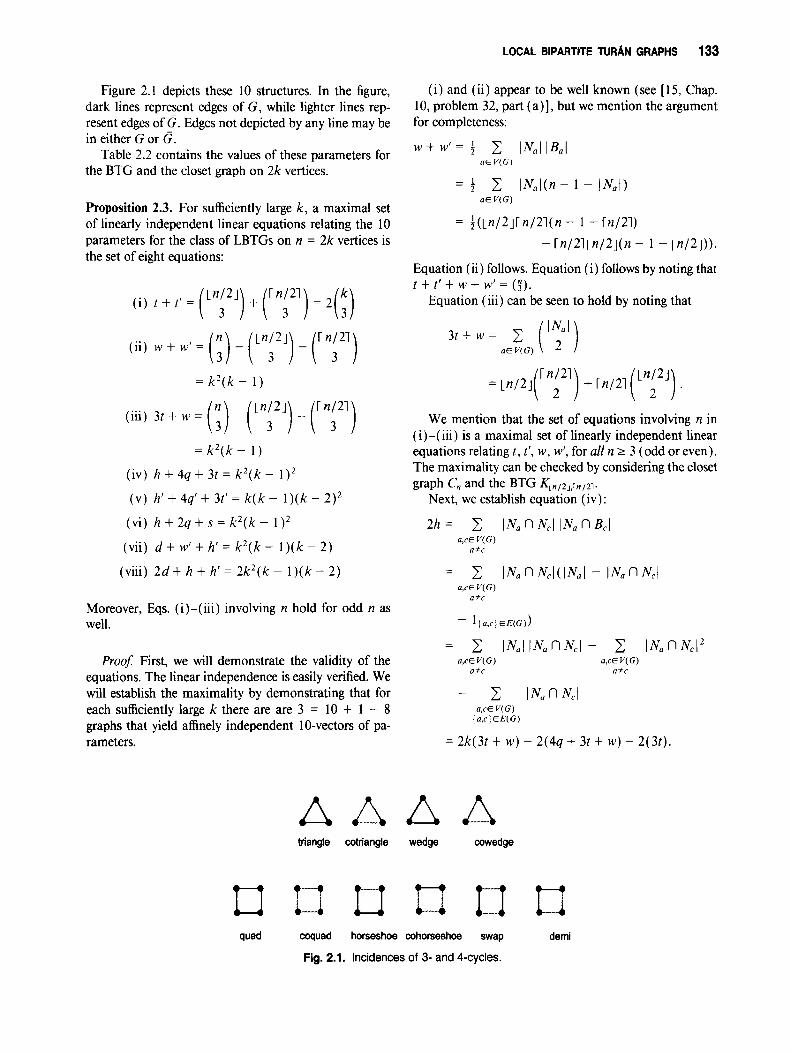
p ( p ) = p( ?r( p ) ) , we have essentially four distinct parameters on strings of length 3 and six on strings of length 4. Let

t ( G ) = p ( G , 111) (the number oftriangles),

t’( G ) = p ( G , 000) (the number of cotriangles),

w(G) = p ( G , 110) (the number of wedges),

w’( G ) = p ( G , 100) (the number of cowedges),

and let

q ( G ) = p (G, 1111) (thenumberofquads),

q’( G ) = p ( G , 0000) (the number of coquads),

h( G ) = p( G , 11 10) (the number of horseshoes),

h’(G) = p ( G , 1000) (the number ofcohorseshoes),

s ( G ) = p ( G , 1010) (the number ofswaps),

d( G ) = p ( G , 1100) (the number of dernis).

Fig. 1.2. A balanced vertex expansion of C6.

LOCAL BIPARTITE TURAN GRAPHS 133

Figure 2.1 depicts these 10 structures. In the figure, dark lines represent edges of G, while lighter lines represent edges of G. Edges not depicted by any line may be in either G or G.

Table 2.2 contains the values of these parameters for the BTG and the closet graph on 2k vertices.

Proposition 2.3. For sufficiently large k, a maximal set of linearly independent linear equations relating the 10 parameters for the class of LBTGs on n = 2k vertices is the set of eight equations:

= k ' ( k - 1)

(iii) 3 t + w = ( l ) - ( p / 2 J ) - ( ~ 2 1 ) = k'(k - 1 )

( iv) h + 4q + 3t = k'(k - 1 ) '

( v ) h' + 44 + 3t' = k ( k - I)(k - 2)'

(vi) h + 2q + s = k2(k - 1) '

(vii) d + w'+ h' = k 2 ( k - l ) ( k - 2)

(viii) 2 d + h + h ' = 2 k z ( k - l ) ( k - 2 )

Moreover, Eqs. (i)-(iii) involving n hold for odd n as well.

Proof: First, we will demonstrate the validity of the equations. The linear independence is easily verified. We will establish the maximality by demonstrating that for each sufficiently large k there are are 3 = 10 + 1 - 8 graphs that yield affinely independent 1 0-vectors of parameters.

Ll quad

(i) and (ii) appear to be well known (see [15, Chap. 10, problem 32, part (a)] , but we mention the argument for completeness:

w + wI= f 2 lNal lBal a € V ( G )

= 5 C INaI(n- 1 - I N a I ) a € V ( G )

= f(p/qr n/21(n - 1 - rn/21) - r n / 2 i ~ n / 2 ~ ( n - 1 - p / 2 J ) ) .

Equation (ii) follows. Equation ( i ) follows by noting that t + t' + w + w' = (!).

Equation (iii) can be seen to hold by noting that

3 t + w = C (Iy) a€ V( G )

We mention that the set of equations involving n in ( i ) - ( iii) is a maximal set of linearly independent linear equations relating t , t', w , w', for all n 2 3 (odd or even). The maximality can be checked by considering the closet graph C,, and the BTG K ; , , / 2 , , l n / 2 1 .

Next, we establish equation (iv):

2h = C I N a n N c I I N a n B c I a,cE V ( G )

a f c

= C I N a n N c I ( I N a 1 - I N a n N c l a,c€V(G)

a2c

- l { a , c } € E ( G ) )

= C I N a I I N a n N c I - C I N a n N c I ' a,& V ( G ) a,& V( G )

aZc afc

- C I N a n N c I a,cE V ( G ) i a,c i EE(G)

= 2k( 3t + W ) - 2(4q t 32 + W ) - 2( 3 t ) .

triangle cotriengle

t'-? L--4 coquad

Fig. 2.1.

Ilf wedge cowedge

horseshoe cohorseshoe swap demi

Incidences of 3- and 4-cycles.

134 LEE AND RYAN

Equation (iv) follows by appealing to (iii) . The proof of (v) is similar to that of (iv):

Equation (v) follows by noticing (iii) 3t’ + w’ = 3 ( t + t ’ ) = k ( k - l ) ( k - 2 ) .

Next, we derive (vi):

4h + 8q + 4s

Using (iii), we obtain (vi). Next, we verify (vii):

TABLE 2.2. Parameter values for the BTG and closet graph on 2k vertices

Parameter C 2 k

t t‘ W

W’

4

4’ h h‘

d S


It is straightforward to check that (i)-(viii) are linearly independent. For example, we can observe that (i)-( viii) is equivalent to the set

(ii’) w’ = 3t

(iii’) w = k 2 ( k - 1 ) - 3t

(iv’) q = t ( k 2 ( k - - 3t - h )

(v’) h’ = h - 6t

(vi’) s = f ( k 2 ( k - + 3t - h )

(vii‘) d = k 2 ( k - l ) ( k - 2) t 3t - h

(viii’) q‘ = : ( k ( k - l ) ( k - 2 ) ( k - 3) + 9t - h ) .

To verify that any other linear equation relating the 10 parameters is a linear combination of these eight equations (for sufficiently large k ) , we present three graphs, for each sufficiently large k , having affinely independent 10-vectors of parameters. In fact, it is enough to demonstrate that the three 2-vectors ( t , h ) are affinely independent. Two of the graphs are familiar: the closet graph

gether from ck(w, w’) and Krk121 ,Lk lZ , . Let ( L , H ) be the natural vertex bipartition associated with & k / 2 1 , ~ k / 2 ~

= Tk/21, /HI = ~ k / 2 ~ . ) If k is odd, let U = L ( c k ) and let U’ = H ( Ck). If k is even, let U = Wand let U’ = W’. The graph & is formed from the union of c k and K r k / 2 1 , ~ k / ~ , , together with all possible edges between U and L , and all possible edges between U’ and H . The graph

hence, it is an LBTG. See Figure 2.4 for drawings of GI2 and GI4 .

For a nonnegative integer I , we say that a function of k is q k ’ ) if the function is bounded from above and below by polynomials of order 1. Since G 2 k contains c k , we have

C 2 k and the BTG K k , k . The third graph 6 2 , is pieced to-

E ( & k / Z l , ~ k / 2 j [ L ] ) = E ( K r k / 2 1 , ~ k / 2 ~ [ H I ) = 0, I LI

G 2 k iS a CrOSS product Of ck(w, w’) and I ( k / 2 1 , ~ k / ? , ;

that t ( G 2 k ) is O( k 3 ) . It is clear that h( 6 2 k ) is O( k4) since most choices of four vertices, one from each of L , H , W, and W’, induce a unique horseshoe of 6 2 k . Now considering Table 2.2, we have

t [ O(k3) c; 0 @:it)) h O ( k 3 ) 0 O(k4)

1

The determinant of this matrix is Q( k ’ ) , which is non- I zero for sufficiently large k . The result follows.

With respect to the statement of Proposition 2.3, k 2 4 is probably sufficiently large. There is probably a generalization of Proposition 2.3(iv)-(viii) for odd values of n , but the counting arguments appear to become quite messy.

A sharp lower bound on t( G) is 0, which is achieved by (and only by) BTGs. We also have the following:

Corollary 2.5. A sharp upper bound on t( G ) for the set of LBTG on n vertices is

ProoJ: That t ( G ) I (L7/2J) t ( r ! / 2 1 ) is immediate from Proposition 2.3(i). The LBTG C, attains the bound of the result.

We remark that closet graphs are not the only graphs that attain the bound of Corollary 2.5. Proposition 4.12 indicates how all such graphs can be constructed. Also, the existence of the closet graphs establishes that there is at least a factor of approximately (n/2)! more LBTGs than BTGs on n vertices.

Corollary 2.6. If G is an LBTG on 2k vertices, then

J

Fig. 2.4. Two cross products.

136 LEE AND RYAN

Proposition 3.2. Let G be an LBTG on n vertices. If t ( G) > 0, then G contains at least ( n - 7)/2 triangles if n is odd and at least n - 4 triangles if n is even.

with equality if and only if G is isomorphic to Kk,k. Proof: Let T be the vertices of a triangle of G. First, we will demonstrate that G contains at least 3 ~ n / 2 J - n - 2 triangles that share an edge of G [ r] . Let C[ TI denote the edges of G that have one endpoint in T . Clearly, IC[T]I 2 3 ( ~ n / 2 ~ - 2). Let Sj denote the subset of V ( G)\T that is met by j edges from C [ TI ( j = 0, 1, 2,

3). Clearly, I C[ TI I = C I Sj I j . Every element of S2

Proof: The inequality is immediate from (iv) . If equality holds, then t = 0. The result follows from Turin’s Theorem.

Corollary 2.7. If G is an LBTG on 2k vertices, then 3

j=O

d ( G ) I k2(k - I)(k - 2)

with equality if and only if G is isomorphic to Kk,k.

Proof: The inequality is immediate from (vii). If equality holds, then w’ = 0. This implies that w = k2( k - 1 ) by (ii). This, in turn, implies t = 0 by (iii). Then, the result follows from TurLn’s Theorem.

Corollary 2.8. If G is an LBTG on 2k vertices, then

413t(G) + h(G).

induces one triangle with its two neighbors in T . Every element of S3 induces three triangles with its three neighbors in T. Elements of So U SI induce no triangles with edges in G[ TI. Hence, the number of triangles of G that share an edge with G[ TI is 1 + I S2 I + 3 I S, I. Therefore, the number of triangles of G that share an edge with G [ TI isatleast3(Ln/2]-2)+ 1 -( lS, l + IS21).Now, ISII + I S, 1 5 1 V ( G)\ TI = n - 3. So the number of triangles that have an edge in common with G[ TI is at least 3Ln/ 21 - n - 2. If n is odd, this bound is precisely ( n - 7 ) / 2. For the case in which n is even, G contains two disjoint triangles by Lemma 3.1. But twice the established bound is precisely n - 4, when n is even.

In particular, if t( G) = t( C 2 k ) , then We remark that the bounds of Proposition 3.2 are sharp

for all n . Furthermore, Proposition 3.2 is not implied by integrality and nonnegativity restrictions imposed on so- lutions to (i)-(viii) of Proposition 2.3, even for n = 2k = 6, since the unique solution having t = 1 and h = 9 is integer valued and nonnegative; this is easily verified using (i’)-( viii’) from the proof of Proposition 2.3.

if k # 3, 7, l l , 15, 19, * - - “{:::;’+ 2, if k = 3, 7, 11, 15, 19,. . . .

Proof: Follows from (iv).

3. MORE ON THE TRIANGLE STRUCTURE

Lemma 3.1. Let G be an LBTG on n vertices, with n even. If t(G) > 0, then G contains at least two disjoint triangles.

Proof: Suppose that n = 2k, and let T be a set of 3 vertices such that G[ TI is a triangle of G. Clearly, G [ V(G)\T] contains exactly k2 - 3(k - 2) - 3 = k2 - 3k + 3 edges. Now G[ V(G)\T] has 2k - 3 vertices, so, by TurLn’s Theorem, if it has more than ~ ( 2 k - 3)/ 2 ~ r ( 2 k - 3)/21 = k2 - 3k + 2 edges (which it does), then it must contain a triangle. Since G[ TI and G[ V ( G)\ TI are disjoint, we have established the result.

This result does not hold in the odd case. Lemma 3.1 is sharp (for all even n ) in the sense that there are LBTGs on n vertices ( n even) with t( G) > 0, but without three mutually disjoint triangles.

4. DECREASING THE NUMBER OF TRIANGLES

Turin’s Theorem and Corollaries 2.6 and 2.7 give three natural measures of proximity of an LBTG to the set of BTGs (on a fixed, even number of vertices), namely, LBTGs with (relatively) low values of t( G), - d( G) and -q(G) are close to the set of BTGs. The content of the aforementioned results is that these three quantities are minimized by, and only by, BTGs. It is natural to study how we might pass from an LBTG with these quantities not minimized to a BTG, using some simple operation that allows us to remain in the class of LBTGs, such that the value of some simple increasing function of these three quantities is nonincreasing. There are many candidates for the operation and the function. Considering Turin’s Theorem, the most natural function to examine is t( G) and the simplest operation is a “swap.”

Suppose that a, b, c, and d are distinct vertices of G such that { a , b } and {c, d } areinE(G), and { a , d } and


( h . c} are not in E ( G ) . Let G,, be defined by V ( G , , ) = V ( G ) and E(G,,,,)) = E ( G ) \ { { a , b } , { c , d } } U { { a , d } . {b,c}}.Then, G,,arisesfromGbyaswup. Any simple graph can be transformed into any other graph (on the same set of vertices) with the same degrees by a sequence ofswaps (see, e.g., [ I , pp. 151-1521).

Proposition 4.1. Let G be an LBTG on n vertices. If G,, arises from G by a swap, then t ( Gsw) 2 t( G ) - 2r 12/21 + 4.

Proof: Suppose that a, b, c, and dare as in the definition of a swap. The net decrease in the number of triangles is equal to

Now,

But notice that if { a , c } E E( G), then

Hence,

Similarly,

It is also easy to see that

Tn/21, if d E H ,

Ln/2J, if d E L .

if I { a , d } n L I = 2 ;

if I { a , d } n L I = 1;

if l { a , d } nLI = 0 ,

-rn/21, if I { b , c } n L I = 2 ; if I { b , c } nLI = 1;

- [n/2j , if I {b , c } n LI = 0.

The result follows by considering the possible degrees of a, b , c, and d. For example, the net decrease in the number of triangles can be as large as 2f n / 21 - 4 if a , h, c, and dare all in L .

We remark that the bound of Proposition 4. I is sharp for all n .

Corollary 4.2. Let G be an LBTG on n vertices. The total number of swaps required to pass from G to a BTG is at least t(G)/(2Tn/21- 4) .

Corollary 4.2 implies that at least ( 9 / 3 swaps are required to transform the closet graph C2k into any BTG Kk,k . We derive a stronger lower bound (Corollary 4.5) as a consequence of the following: Let F and F ' be arbitrary simple graphs having V ( F ) = V ( F ' ) and having the degree of each vertex be the same in F and F'. Let a( F , F ' ) denote the minimum number of swaps needed to transform F into F'.

Proposition 4.3.

Proof.' E( F ) A E ( F ' ) is the (nonunique) union of (edge-) disjoint alternating circuits (i.e., (not necessarily simple) circuits the edges of which alternate between those of F and those ofF') (see, e.g., [ l , p. 1501). Suppose that there are p such circuits Q,, 1 I i I p , in some such decomposition; let the lengths of these circuits be 1, 2 4, and even, 1 I i I p . A transfer from F to FAE( Q, ) can be effected by a sequence of (1, /2 ) - 1 swaps. Hence, a lower bound on the number of swaps is

P min 2 (k- 1 ) .

I = 1

where the minimum is taken over values of I, and p sat- isfying

A lower bound on the minimum arises by thinking of p = I E( F ) AE( F ' ) I /4 and I, = 4 for all i (we may not be able to achieve this exactly if 4 does not divide I E( F ) BE( F ' ) I ). On the other hand, the maximum is achieved with p = 1 and 1, = I E( F ) AE( F ' ) I . The result follows.

138 LEE AND RYAN

Corollary 4.4. Let G and G’ be LBTGs on 2k vertices:

u(G, G’) I 2( :) - 1.

Proox Follows from Proposition 4.3 by observing that IE(G)AE(G‘)I I 4($).

Define the same-cut Kk,k relative to the closet graph C 2 k ( W , W ’ ) to be the BTG determined by the partition (W, W’). We note that the inequality in the proof of Corollary 4.4 is sharp by considering G to be a closet graph and G’ to be its same-cut Kk,k. For specificity, let W = { w I , w2,. . . , wk} and W‘ = { w’,, wi, . . . , w;(} be indexed in such a way that { { wi , w: } : 1 I i I k} is the set of independent edges connecting W to W‘. Define a crosscut Kk,k relative to C 2 k ( W , W ’ ) to be a BTG determined by the partition of the vertex set into

{ w , : i = O m o d 2 } U { w ; : i = 1 m o d 2 )

and

{ w; : i = 1 mod 2 ) U { w: : i = 0 mod 2 ) .

Note that a given closet graph has many different crosscuts as there are many ways to label the elements of W.

Corollary 4.5.

Proox Consider the minimum value of 1 E( C 2 k )

minimum is achieved by choosing a crosscut K k , k of c 2 k .

The result follows.

&??( &,k) I 14, with C 2 k fixed but K k , k allowed to Vary. The

Corollary 4.6. For each closet graph C 2 k , there exists a Kk,k on the same vertex set such that for any sequence of swaps between the two graphs, the average decrease in the number of triangles per swap is no greater than $( k - 1 ) [as compared to the maximum decrease attainable of 2k - 4 (see Proposition 4.1 ) ] .

On the other hand, relatively long sequences of swaps of maximum decrease are possible. Suppose that F k is the BTG having vertex bipartition ( { 1, 2, . . . , k} , { 1 ‘, 2’, . . . , k’} ). For any distinct i, j between 1 and k, let Fk( i, j ) denote the graph arising from Fk by swapping { i, j ’ } and { j , i’} out for { i, j } and { i’, j ’ } . Assume that k is even, and consider the graph (abusing notation slightly) (( Fk( 1,2))( 3,4) - - - )( k - 1, k). “Undoing” these swaps gives a sequence of k/2 swaps with triangle decrease of 2k - 4 per swap.

We can also demonstrate that it is possible to pass from a closet graph to a BTG using only triangle-decreasing swaps. In doing so, we demonstrate that there are classes of LBTGs on 2k vertices that admit sequences of a( k2) triangle-decreasing swaps. It would be interesting to find a class of examples that would improve this lower bound to Q(k3).

Proposition 4.7. Beginning with the closet graph G = C2k(A, B ) , there is a sequence of triangle decreasing swaps leading to a BTG G’, having bipartition (A‘ , B’) with the following properties:

(i) G‘[A] and G’[B] are isomorphic to K r k , 2 1 , ~ k / 2 , .

(ii) Letting ( A l , A 2 ) [resp., ( B l , B2)] be the natural vertex bipartition of G’[A] (G‘[B] ) , with I A I I

natural vertex bipartition ofthe BTG G’[A1 U B 1 ] ( G ’ [ A 2 U B 2 ] ) , and A’ = A l U Bz, B’ = A2 U BI .

(iii) BI is the set of vertices in B that are each adjacent, in the graph G , to a vertex in A l .

I l A 2 l ( l ~ l l 2 1 & 1 ) , (A19 Bl) Iresp.3 (A29 B2)l is the

Moreover, every swap in the sequence consists of deleting edges in G [ A ] and G [ B ] , and adding only edges that cross between A and B . In particular, if e = ( v , u ’ ) E E( G ) , with u E A and u’ E B , then e remains an edge throughout the sequence of swaps.

Proof The proof is by induction on k. The result is easily checked fork = 3; indeed, only one swap is required. Assume that the result holds for all closet graphs C2, with 1 < k .

Let G = c2k(A, B ) . Choose an edge e = ( w , w’) that crosses between A and B in G . By the inductive hypothesis, the subcloset graph H = G [ A U B\ { w, w ’ } ] can be swapped into a bipartite graph H’ as in the statement of the theorem. Since the number of triangles is decreasing within the subcloset, and since (by the “moreover” part of the proposition) triangles involving w and w’ are only being destroyed, this sequence of swaps is triangle decreasing with respect to G.

For convenience, let A I , A 2 , BI , B2 be defined as in the statement of the proposition, but with respect to H . Our goal is to perform further swaps that are triangle decreasing with respect to G , to arrive at G‘, so as to add w to A l and w’ to B, , and so that all sets are as advertised in the statement of the proposition. Note that w (resp., w’) is added to A I ( B1 ) that is the smaller of A I and A2 ( BI and B2) so as to maintain balance.

At this stage, the entire graph has


triangles, each of which contains w or w’. Now for each u E A , , perform the following swap involving w, w’, u, u‘: Add edges ( M’. v‘), (MI’, u ) and delete edges (w, v ) , (w’, u ‘ ) . Since ( w , L V ’ ) , and ( u , u’) are edges. the net decrease in the number of triangles is

Note that N , fl Nor = $3 and that every vertex of H is adjacent to u or u’. Hence, IN,, fl N , I + I N,, n N,! I = IN,, 1 =k.Similarly, IN,,,nN,J + IN,,,nN,tI = IN,b,I = k . Also, by symmetry, 1 N,, fl N, I = I N,, I n Nut 1 . So the net change in the number of triangles is

Consider 1 N,, fl N, I . Initially, IN,, n N, I = T(k - 1 )/ 21. But at the ith swap, I - 1 other vertices u‘ E BI have been made adjacent to w. These vertices are all adjacent to u, since ( A I , BI ) is complete bipartite. I N , f l N, I does not decrease, since the only edges incident to w that are deleted are vertices in A l , which is not adjacent to [since ( A l , .4*) is a complete balanced bipartite graph]. Thus, at the ith swap, IN,, n N,I = r (k - 1)/21+ 1 - 1.

Thus, at the ith swap (after H has been created), the net decrease in the number of triangles is

which is always positive. We perform the swaps for all v E A ,, so i I L ( k - 1 ) / 2 J. Note that summing ( * ) over i between 1 and ~ ( k - 1)/2J results in 21(k - 1)/2~T(k - 1 )/21, as expected, so all of the triangles are eliminated. It is easy to check that the final graph G’ is as desired. I

Note that the operations described in the proof of

Proposition 4.7 give rise to a sequence of C L( I - 1 ) / 2 J

swaps. If k is even, this expression is equal to k ( k - 2 ) / 4 and the lower bound of Corollary 4.5 is obtained. It is interesting to observe that G‘ is a crosscut BTG of G; hence, it is a BTG that has as many edges in common with G as possible.

Suppose that n is odd and that a is in L( G) and b is in H ( G ) . There is some vertex c that is in Nb\N,. Let Glh be defined by V(G,h) = V ( G ) and E(Gsh) = E ( G ) U { a , c} \ { b , c}. Then, Gsh arises from G by a shift. If G’ is another LBTG with V ( G’) = V ( G ) , then G can be transformed into a graph with the same degrees as G’ with a sequence of [no more than ( n - 1 ) / 2 ] shifts. We can

h

I= 3

complete the transformation of G into G‘ with a sequence of swaps.

Proposition 4.8. Let G be an LBTG on n vertices, with n odd. If Gsh arises from G by a shift, then t( Gxh) 2 t ( G) - ( n - 5 ) / 2 .

Proof: Suppose that a , b , c are as in the definition of a shift. The net decrease in the number of triangles is equal to

Now INh f l N,I is bounded above by ( 1 7 - 1) /2 if c’ E H ( G ) and by ( n - 3 ) / 2 if c E L ( G ) . It is easy to see that IN, fl N, I is bounded below by 3 if c E H ( G ) and by 2 if c E L ( G ) . So in either case, INb fl N,I - INu n N, I is bounded above by ( n - 7 ) / 2 . The result follows. I

We remark that Proposition 4.8 is sharp for all n . The following class of examples show that there are

LBTGs for which every swap strictly increases the number of triangles.

Example 4.9. Let A , B , and C be the tripartition of a complete tripartite graph. Similarly, let A‘, B’, and C’ form another complete tripartite graph, and let I A1 = IA’I = q , IBI = /B’I = r , and (CI = IC’I = p . Now, letA and A’ be the bipartition of a complete bipartite graph, and, similarly, let B and B’, and C and C‘, form complete bipartite graphs. Together these define an LBTG on 2k nodes, with k = 4 + r + p . Note that this graph is a balanced vertex expansion of the closet graph C, (see Sec- tion 1 andFig. 1 . 2 ) . S u p p o s e t h a t i 2 2 a n d z ~ j + I - 3 for all combinations of I . J , 1 E { r , p , 4 } . In particular, if r = p = 4 2 3 , these inequalities all hold.

We now consider the possible swaps: Suppose that the swap involves adding the edges (u , w) and (x, y ) , and deleting the edges ( u , x) and (w, y ) .

CASE I . Suppose that v and w are contained in the same isolated set A , B , C , A’, B’, or C’. Without loss of generality (the argument here easily generalizes to any isolated set), assume that they are both in A . Then, either ( i ) x and y are both in A‘. or ( i i ) x and y are both in B (or C), or (iii) one of them is in A‘ and the other is in B (or C). In subcase ( i ) , it is easy to see that the number of triangles strictly increases.

In subcase (i i) , suppose that x and y are both in B ; the case where they are both in Cis similar. Then, I N ,

= 1 N , fl N,, I . Since both ( u , y ) and ( w, x) are edges, the net decrease in the number of triangles is

nN, l = q + r + p = IN,rlN,,I,and IN,nN,l = p

140 LEE AND RYAN

wU n N,I + IN, n ~~i - IN, n N,I - IN, n ~~i + 4 = 2 p - 2 ( q + p + r ) + 4 = -2(q + Y) + 4 < 0.

So, the number of triangles strictly increases. In subcase (iii), (say x E A’ and y E B ) , we have

that again IN, n N,I = q + r + pand N , n Ny = p , butthat IN,nN,,I = q + r , a n d IN,nN,I =O.Since ( u , y ) and (w, x) are edges, the net decrease in the number of triangles is

IN” n N X I + IN, n Nyl - IN, n NWI - IN, n N y l

+ 4 = p - ( q + p + r ) - ( q + r )

+ 4 = -2(q + r ) + 4 < 0.

So, the number of triangles strictly increases.

CASE 2. Suppose, without loss of generality, that u E A and w E B’. (The cases where v and w are in other isolated sets can be proved similarly.) Then, either (i) x E A’, or (ii) x E B , or (iii) x E C. In subcase (i), since (w, y ) is an edge and since (x, y ) is not, it must be that y E B. In this case, no triangles are deleted, and many are added, so the number of triangles strictly increases.

In subcase (ii), since (x, y ) is not an edge, and since (w, y ) is an edge, either y E B , or y E A’, or y E C’. If y E B , then since x and y are in the same isolated sets, this reduces to Case 1 with (x, y ) playing the role of(u,w).IfyinA’,then INunNwI = INxnNyI = q + r a n d IN,nN,I = IN,nNyI =p.Since(u,y)and (w, x) are both edges, the net decrease in the number of triangles is

So, the number of triangles strictly increases. If y E C’, then we still have I Nu fl N , I = q t Y and

IN, n N,I = p , but N , f l Ny = q and IN, n Nyl = r + p . Since (w, x) is an edge, the net decrease in the number of triangles is

INUnKI + INwnNyI - I N u f l N w I - IN,nNyI + 2 = p + q - ( q + r ) - ( r + p )

+ 2 = - 2 r + 2 < 0 .

So, the number of triangles strictly increases. In subcase (iii), since (x, y ) is not an edge, and ( w,

y ) is an edge, it must be that y E A’. In this case, I Nu nNWI = q + r , IN,nN,,I = p + q , IN,nN,I = r ,

and I N , n Ny I = p . Since ( u , y ) is an edge, the net decrease in the number of triangles is

wU n N,I + IN, n ~~i - IN, n N,I - IN^ n N ~ I + 2 = p + r - ( q + r ) - ( p + q )

+ 2 = -2q + 2 < 0.

So, the number of triangles strictly increases.

A more general class of merit functions to consider consists of those of the f o m f ( G ) = alt(G) - a2d(G) - a3q( G), where ( al , a2, a3) is semipositive. The following result indicates that for such linear functions we may as well take a3 = 0.

Proposition 4.10. For any choice of semipositive ( al , a2, a3) with a3 positive, there is a choice of semipositive ( a ; , a; ) and a constant a. such that a’, t ( G) - aid( G) = uo + ~ l t ( G ) - ~ 2 d ( G ) - ~3q(G).

Proof: It follows from Proposition 2.3 that 6t - d + 4q = k 2 ( k - I ) . Take dl = al + ;a3, a; = a2 + fa3, and a. = fa3k2(k - 1).

Confining ourselves to functions of the form f( G) = all( G) - a2d( G), with (al , a2) semipositive, we remark that the choices (1, 0), (0 , l ) , and ( 1 , E ) for ( a l , a2) all admit choices of LBTGs G that are not BTGs, but for which there is no choice of swap that decreasesf.

The obvious generalization of a swap is an alternating (even) cycle. If G‘ arises from G by a swap, then GAG’ is an alternating 4-cycle.

Proposition 4.11. If G is an LBTG on an even number of vertices with t( G) > 0, and G’ is any BTG on the same set of vertices, then there is a sequence of LBTGs G = Go, GI, . . . , G, = G’ ( p 2 1 ) on the same vertex set, such that Gi-lAGi is a (not necessarily simple) alternating cycle (with respect to Gj-l and Gi), GiPlAGi is vertex disjoint from Gj-lAGj for all i Zj, and t(Gj-I) > t(Gi), for all 1 I 1 I p .

Proof: The connected components of GAG’ are (vertex disjoint, not necessarily simple) alternating cycles { Ci : i E S = { 1, 2, . . . , p } } (with respect to G and G’) . For each i E S , let 7; = t(GACj) - t(G). Every triangle of the complete graph on V(G) has one or more edges in common with at most one of these cycles. Hence, for any set T C S , t(GA( UiETCi)) = t(G) + C 7 i . Hence, 7,

5 0, for all i E S . Suppose that ~~f = 0, for some i’ E S . Consider the

graph GAjzjtCi. This graph is a BTG, but it differs from G‘. Now it is easy to check that the symmetric difference

iE T


of distinct BTGs (on the same set of vertices) is a connected graph that meets all of the vertices. Hence, p = 1, but then there is no T, < 0, contradicting t( G) > 0. Hence, 7, < 0 for all i E S . Hence. we can let GI = GA,,,,C, for 1 < ; < [ I - 1. I

Note that p I k / 2 in Proposition 4.1 I . Consider an infinite family of graphs with t( G) = R( k*+‘). It cannot be that the length of all alternating cycles constructed using the method in the proof of Proposition 4.1 1 have length bounded by a constant, since any such cycle can only reduce the number of triangles by O ( k ) .

By the construction in the proof of Proposition 4.1 I , for any LBTG G with t ( G ) > 0, it is easy to find an alternating cycle C (with respect to G ) such that t( GAC) < t ( G ) . The more difficult problem is to find such a C to minimize a C c(e) + t(GAC)?, where

c : E( K,,) + 91, for some fixed cy 2 0 and y 2 1. A similar proof establishes the following:

P€E( G X ’ )

Proposition 4.12. If G and G’ are distinct LBTGs with t ( G ) = / ( G’) extremized [ i.e., either 0 or 2 (:)I, then there isa sequence of LBTGs G = Go, G , , . . . , Gp = G ‘ ( p 2 1 ) on the same vertex set, such that G,-,AG, is a (not necessarily simple) alternating cycle (with respect to GI- , and G I ) . G,-,AG, is vertex disjoint from GJ_,AG, f o r a l l i f / . a n d f ( G , ) = t ( G ) = t ( G ’ ) , f o r a l l O s i s p . Moreover, if t ( G) = t( G’) = 0, then p = I .

5. A LAYOUT HEURISTIC

In this section, we present a new heuristic for a VLSI circuit layout problem. Suppose that c : E( K,,) * % [also for S C E. we write c ( S ) for C c ( e ) ] . We want to find

a spanning BTG G of K,, that has minimum total weight (by a spanning BTG of K,,, we mean a BTG G that is a subgraph of K,, and has V ( G) = V ( K,,)] . The problem arises when we wish to place electrical components on two circuit boards, so as to balance the number of components on the two boards, while minimizing the total cost of interboard connections. This layout problem is NP-complete (see [ 5 I ) . Cutting-plane methods of integer programming have been proposed for this problem (see [ 3.4, 131). In addition to cutting plane methods, bounds can be obtained by eigenvalue methods (see, e.g., [2]) . Vertex interchange heuristics starting from an arbitrary spanning BTG of K,, have met with some success (see [ 9- 11 , 141 and the references therein). Let S, be the set of spanning LBTGs of K,,. For simplicity, we will assume that n = 2k.

e € S

An Edge-Swapping-Based Heuristic

1. Start with G E to minimize c( E( C ) ) . We can find such a subgraph using Edmonds’ matching algorithm (see [ 161). The weight of G is a lower bound on the optimal solution.

2. Choose cy 2 0. and y 2 I . 3. Starting with F = G , perform swaps to find a local

minimum of the merit function

over F E S z x . Let G be the resulting graph. 4. If t ( G) > 0 and a > 0, then decrease a just below the

level at which some swap will decrease the merit function (setting cy = 0 if there is no such nonnegative level) and return to (3) . If t ( C ) > 0 and a = 0, then g o t o ( 5 ) . I f t ( G ) = O , t h e n g o t o ( 8 ) .

5. Starting with G, perform one swap to maintain the number of triangles, but increase the number of demis. Let G be the result and return to (3) (recall CY = 0) . If no such swap is available, then go to (6) .

6. Choose e E E ( G ) , such that e has maximum weight among edges on odd cycles of G, and let G + ( V ( G) , E( C)\e). If G is not bipartite then return to (6) .

7. G is now bipartite. Let ( L , H ) be a bipartition of V ( G) such that every element of E( G) crosses the bipartition. Assume, without loss of generality, that I LI 2 ( H I . If I L I = I H I = k , then go to (8 ) ; otherwise, greedily, based on the total cost of all edges of K2k that cross the bipartition. transfer a vertex from L to Hand return to ( 7 ) .

8. G is now a spanning BTG. Starting with G, use a vertex- interchange procedure, maintaining the bipartite Turin property, until the cost cannot be reduced. For example, interchanges might be restricted to verfex- swaps (choose a E Hand b E L , and let H + H\ { a } U { b } , L + L\{b} U { a } ) , or we might use the heuristic of Kernighan and Lin [ lo] .

9. Output the BTG determined by the partition ( L , H ) .

Without performing extensive large-scale experiments, we wanted to get some idea of the potential power of edge swapping as compared to vertex interchange methods. We did not attempt to demonstrate that a particular heuristic based on edge swapping (and there are many variations on the above heuristic using concepts of simulated annealing and tabu search, e.g.) outperforms a particular heuristic based on vertex interchange methods. Indeed, the best methods may be a hybrid heuristic.

We applied steps ( 1 ) - (4) of the heuristic (with y = 1 ) to a set of 10 random problems each having n = 80 vertices. In all runs, whenever we perform an edge

142 LEE AND RYAN

swap, we seek the maximum decrease in the merit function. All 10 problems have “geometric cost functions” (see [ 91). A geometric cost function arises by associating a vertex with each element of a finite set of points in the plane. The cost of the edge between a pair of vertices is 1 if their Euclidean distance is less than some threshold 4 and 0 otherwise. If n points are uniformly and indepen- dently distributed in the unit square, then the expected cost of the edges meeting a vertex not near the boundary of the square is approximately n?r42. Such problems have natural clusters of points that are geometrically close and appear on the same side of an optimal partition. We chose 4 = .148677; hence, our graphs are expected to be rather sparse, having n?r4’ x 5.6. As compared to the test problems of Johnson et al. [ 91, the number of vertices is quite small. On the other hand, as integer linear programs, these are nontrivial problems having (”) = 3160 variables. Furthermore, the obvious formulation has 80 + (’!) = 82,220 constraints and the linear programming relax- ation is highly degenerate.

For each problem, we made the following runs: (i) edge swapping [ i.e., steps ( 1 )-(4) of the new heuristic], followed by the Kernighan-Lin Heuristic, and (ii) 100 repetitions of the Kernighan-Lin Heuristic, starting from randomly generated balanced bipartitions.

We have made little effort to eficientfy implement edge swapping, though we can make the qualitative statement that edge swapping appears to be much more time-consuming than is vertex swapping. The heuristics were coded in FORTRAN 77 an run on a SUN SparcStation. The minimum-weight k-factor problems [step ( 1 )] were solved with the XPRESS Branch and Bound code. In all 10 instances, the minimum-weight k-factor had 0 edge cost.

Table 5.1 summarizes the results. For each of the 10 problems, we have tabulated the minimum, maximum, and mean cost for both the 100 initial random bipartitions and the 100 outputs of the Kernighan-Lin Heuristic. For both means, we have also included the standard errors, so as to demonstrate that these sample means are expected to be quite close to the underlying population means. The column labeled “r2” contains the squared correlation coefficients between the cost of the initial partitions and the cost of the output of the Kernighan-Lin Heuristic. Under “EDGE SWAP” is tabulated the cost of the initial bipartition produced by edge swapping, as well as the output of the Kernighan-Lin Heuristic, beginning from this bipartition.

The Kernighan-Lin Heuristic is quite sensitive to the initial partition. This variability can be exploited by performing several runs and choosing the best one obtained (see [9]). Indeed, for each of our 10 problems, the best solution obtained beginning from a random bipartition, always out performed the solution obtained starting from the solution obtained by edge swapping.

TABLE 5.1. Result summary

RANDOM

INIT K- L EDGE SWAP

Min x Min 8 No. Max (S2) Max ( S f ) r2 INIT K-L

1

2

3

4

5

6

7

8

9

10

69 I14

83 117

68 98

79 109

71 105

67 105

68 105

80 107

80 110

72 107

99.54 (.728)

102.61 (.625)

87.18 (.668)

94.82 (.744)

93.1 1 (.665)

87.79 (.732)

84.84 (.663)

95.45 (.612)

97.29 (.685)

94.36 (.685)

4 14

2 19

1 15

4 12

5 7

1 4

4 4

3 19

5 14

4 17

6.99 .01 (.226)

6.28 .01 (.535)

5.40 .OO (.289)

6.44 .OO (.157)

7.62 .OO (.279)

4.65 .01 (.246)

5.99 .oo (.194)

7.04 .01 (.364)

8.00 .OO (.232)

5.68 .OO (.242)

86 7

60 5

66 2

43 6

58 6

68 7

77 4

54 6

66 10

75 5

However, there are some positive observations: First, in all 10 instances, edge swapping terminated with a bipartition. Second, edge swapping gives initial bipartitions with much lower cost than average random bipartitions. Third, although r 2 , the fraction of the variation in the output of the Kernighan-Lin Heuristic (linearly) ex- plained by the initial random partitions, is always near zero, the initial partitions determined by edge swapping do appear to lead to better than average output from the Kernighan-Lin Heuristic. Indeed, a one-tailed paired t- test of the null hypothesis that there is equality between the underlying means of the Kernighan-Lin Heuristic applied to the output of edge swapping and of the Ker- nighan-Lin Heuristic applied to a random partition has a p-value = 0.1489, i.e., there is less than a 15% chance that the observed data resulted from populations with equal means (defending against the alternative that it is better to begin with the output of edge swapping). Finally, only once did preprocessing with edge swapping lead the Kernighan-Lin Heuristic to a solution that had cost


greater than 50% of the worst solution obtained by the Kernighan-Lin Heuristic started from 100 random bipartitions.

Results appear to be highly sensitive to the cost distri- bution used, but we can make the statement that there is some evidence that for some cost distributions heuristic based on edge swapping may be able to improve upon or be used as initial partition generators for, heuristics based on vertex swapping. The primary obstacle is the running time of edge swapping. More work is needed in this area.

We also tabulated additional statistics regarding the solution paths of the edge-swapping heuristic in Table 5.2. For each of the 10 data sets, we have tabulated the number of triangles of the minimum-weight k-factor found in Step 1 of the heuristic. As a rough measure of comparison, we note that the probability of a random edge being in the selected 40-factor is 40’/( \’) x S0633. Hence, if the triangles were independent of one another (which they are no f ) , we would expect approximately (*!)( ~ 0 6 3 3 ) ~ N 10,665 triangles. We have also tabulated the number of edge swaps used by the heuristic. Since the algorithm allows swaps that increase or maintain the number of triangles, it is not surprising that the average decrease in the number of triangles per swap (around 25) is only about one-third of the maximum decrease in the number of triangles per swap (76). Finally, for each data set, we recorded the least number oftriangles in an LBTG encountered by the algorithm with 0 total edge cost. It is nice to find that edge-swapping can eliminate so many triangles without suffering an increase in the edge cost.

6. A LAGRANGIAN

As an alternative to Step 1 of the edge-swapping heuristic (see Section 5 ), we could let G* be a graph that solves the Lagrangian

where H : ( K 3 C K Z k } + !H, and the minimization is camed out over the set of spanning LBTGs of KZk (see [12]). This method leads to a sharper lower bound on the value of an optimal layout than Step ( 1 ) of the edge- swapping heuristic. We can find such a G* in polynomial time in the following manner:

First, using the ellipsoid method in conjunction with an algorithm of Padberg and Rao [18] (see [6, 7]), we can find optimal dual variables ir corresponding to the “triangle inequalities” of the linear program:

TABLE 5.2. Solution paths of edge swapping heuristic

No. L”,, Swaps I,,, (cost = 0 )

1 2 3 4 5 6 7 8 9

10

13,324 13,208 14,515 13,411 13,810 13.043 13.220 12,131 13,217 14,336

525 479 480 459 467 510 520 454 453 53 I

2830 2070 2256 1582 2260 2284 2590 1840 2558 2497

min 2 c(u)x(e) ,

s.t. ( 1 ) C x(e) = k V u E V ( G ) ,

e t E ( G )

r € 6 ( v )

( 2 ) 2 x, + IF1 - 2 2 xe2 1 v

F C d ( W ) : 1 = k J W I + & 6 ( M ) e€ I.

( 3 ) O s s ( e ) i 1 V e € E ( G ) ,

(4 ) 2 x(e)s 2 V K , C K X . &E( K,)

V C V ( G ) ,

F ( (mod 2) .

Then, we can solve the inner minimization problem of the Lagrangian using Edmonds’ matching algorithm. The validity of this approach depends on the fact that ( 1 )-( 3 ) describes the convex hull of the characteristic vectors of the edge sets of the LBTG subgraphs of K2k (see, e.g., [ 191).

A more practical method of working with the Lagran- gian is by using the subgradient optimization method (see, e.g., [81):

Subgradient Method

1. Choose H I 0 and a target zT . 2. Let G; solve the inner minimization ofthe Lagrangian

and let z , be the value of the Lagrangian with T fixed at ii.

3 . Define the subgradient y by

If y = 0 then stop. 4. Lets = ( z T - z+)/llyl12.

5. If neg(G + sr) = 0. then stop; otherwise, let + +

neg( H + sy ). and go to Step 2.

144 LEE AND RYAN

If zT is chosen to be no larger than the value of the Lagrangian, then z, converges to zT. The computation of I( y 11 in Step 4 would appear to be quite time consuming since y has ( 2 f ) coordinates. The next result establishes that the computation of 11 y 11 is trivial.

Proposition 6.1.

k IM12 = 8( 3) a

ProoJ

= 4( ’:) - 3w‘ - 4w - 3t

=4(’:)-3(w+ w’ ) - (3 t+w)

= 8( ;) , the last equation following from Proposition 2.3 (ii )- (iii ) .

Corollary 6.2. The subgradient lower bounding method can never stop in Step 3.

Next, we provide a family of examples that indicates the potential quality of this Lagrangian lower bound.

Example 6.3. Consider the closet graph C,,( W , W‘) with n = 2k. Consider a crosscut Kk,k of C,,. Let K denote the number of edges of c,, that intersect the edge set of this crosscut Kk,k. We have

K = rk/21(rk/21- 1) + Lk/2J(Lk/2J - 1)

= r k ( k / 2 - 1)l.

Consider the complete graph K,, = C,, 0 c,,. Define c : E(K,,) + 3 by c(e) = leEE(cm) for all e E E(K,,). A minimum-weight spanning LBTG of K,, (with respect to c) is C,,. The weight of E( C,,) is 0. Consider ?r : { K3 C K,, } + defined by ?r( K 3 ) = XKJCc,, , for some nonpositive scalar A. Let

C(e) = c(e) - C ?r(K3) Ve E E(K,,). K3C Kn e€K3

Note that each edge of (each of the two copies of) Kk

(in C,) is contained in k - 2 triangles of Kk. We have

C m) + 2 C 4 K 3 ) e E E ( G ) K3CKn

= -2( :)(k - 2)X + 2 - 2 ( :)” = -2( :)A.

This is a lower bound on a minimum-weight Kk,k subgraph of K,, with respect to c, provided that C,, is a minimum- weight spanning LBTG of K,, with respect to the weight- function C. For an edge e in either of the two copies of Kk, we have C(e) = - X(k - 2) . As long as each of these “transformed costs” is not more than 1, it will be the case that C,, is a minimum-weight spanning LBTG of K,, with respect to C. So let X = - l / ( k - 2). We obtain that the optimal value of the layout problem divided by the (optimal) value of the Lagrangian lower bound is no more than

K r k ( k / 2 - 1)l 3 x - - --

J 2 k ( 2 ) s ( 5 ) 2 ‘

Hence, we have a family of examples for which the value of an optimal layout is within a constant factor of the Lagrangian lower bound, while the ratio of the value of an optimal layout to the lower bound provided by a minimum-weight spanning LBTG is infinite.

7. REMARKS

Although this study is confined to LBTGs, some of the proof ideas can be used to study other classes of simple graphs with few distinct degrees. Of particular interest in the study of VLSI circuit layout are local t-partite Tura‘n graphs (LtTGs), i.e., graphs with the same degrees as t- partite Turin graphs (tTGs) (i.e., complete t-partite graphs on n vertices in which each part has either rn/ t l or Ln/t] vertices). The most obvious measure of closeness of an Lt TG on n vertices to the class oft TGs on n vertices is the number of K,,, subgraphs.

It would be interesting to test a simulated annealing or a tabu search heuristic for the partitioning problem based on the neighborhood and merit ideas of the present paper.

We thank Yves Pochet and an anonymous referee for helpful suggestions based on their careful reading of an earlier version of this manuscript.

REFERENCES

[ l ] C. Berge, Graphs, second revised ed. North-Holland, Amsterdam (1985).


[2] R. B. Boppana, Eigenvalues and graph bisection: An average-case analysis. 28th Annual Symposium on the Foundations Of‘Computer Sciencr (IEEE) ( 1987) 286- 294. M. Conforti, M. R. Rao, and A. Sassano, The equipartition polytope: I , 11. ,Wuth. Program. Ser. A 49 ( 1990/91) 49- 90. C. C. De Souza and M. Laurent, Some new classes of facets for the equicut polytope. CORE Discussion Paper No. 9157 (1991 ).

M. R. Carey, D. S. Johnson, and L. Stockmeyer. Some simplified NP-complete graph problems. Theor. Comput.

[3]

[4]

[5]

Sci. I (1976) 237-267. M. Grotschel. L. LovPsz. and A. Schrijver, The ellipsoid method and its consequences in combinatonal optimization. Combinatorica 1 (1981) 169-197. M. Grotschel. L. Lovasz, and A. Schrijver, Comgendum to “The e h s o i d method and its conseauences in com-

[6]

[7]

binatorial optimization.” Combinatorica 4 ( 1984) 291- 295. N. Held, P. Wolfe, and H. P. Crowder. Validation of subgradient optimization. Math. Program. 6 ( 1974) 62- 88.

[9] D. S. Johnson, C. R. Aragon, L. A. McGeoch, and C. Schevon. Optimization by simulated annealing: An ex- perimental evaluation; part I , graph partitioning. Oper- ations Rex 37 ( 1989) 865-892. B. W. Kernighan and S. Lin, An efficient heuristic procedure for partitioning graphs. Bell Sj,st. Tech. J . 49

[8]

[ 101

(1970) 291-307.

[ I I] S. Kirkpatrick. C. D. Gelatt, Jr., and M. P. Vecchi, Op- timization by simulated annealing. Science 220 ( 1983 )

[ 121 J. Lee. Lower bounds for graph partitioning problems. ORSA/TIMS Joint National Meeting, St. Louis ( 1987).

[ I31 J . Leung, Facets of the balanced bipartition polytope. Yale University Working Paper ( 1988).

[ 141 S. Lin. Effective use of heuristic algorithms in network design. Proceed. Symp. Appl. Math. 26 (1982) 63-84.

[ 151 L. Lovasz, Combinatorial Problems and Exercises. North- Holland, Amsterdam ( I979 ).

67 1-680.

L. Lovisz and M. D. Plummer, Matching Theory North- Holland. Amsterdam ( 1986). W. Mantel. Problem 28, solution by H. Gouwentak, W. Mantel, J. Teixeira de Mattes. F. Schuh, and W. A. Wy- thoff. Wisknndrge Opgaven 10 ( 1907) 60-6 I .

[ 181 M. W. Padberg and M. R. Rao. Odd minimum cut sets and h-matchings. Math. Operations Rex 7 ( 1982) 67- 80.

W. R. Pulleyblank. Polyhedral combinatorics. Mathe- matical Programming, Bonn I992 (A. Bachem, M. Grot- schel, and B. Korte. Eds.). Springer-Verlag, Berlin ( 1983).

[ 191

Received February 1992 Accepted November 1993

Documents

Local bipartite turán graphs and graph partitioning