Embed Size (px)
DESCRIPTION
about load pull simulation using ads
Citation preview

Welcome
1
Andy HowardSenior Applications Engineer Agilent EEsof
2
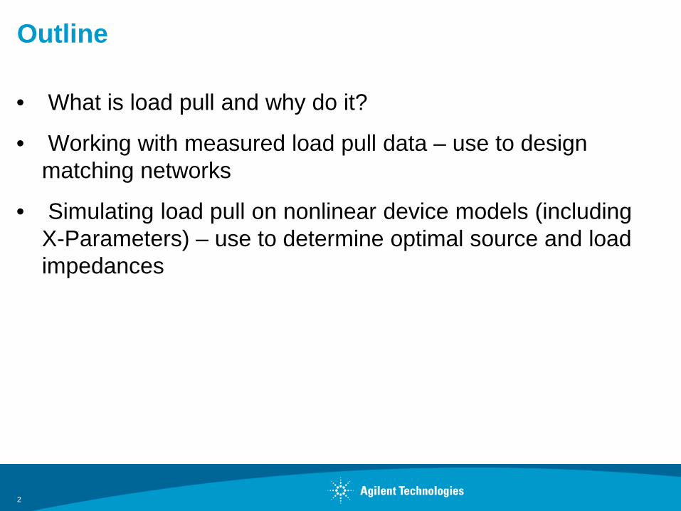
Outline
• What is load pull and why do it?
• Working with measured load pull data – use to design matching networks
• Simulating load pull on nonlinear device models (including X-Parameters) – use to determine optimal source and load impedances
3
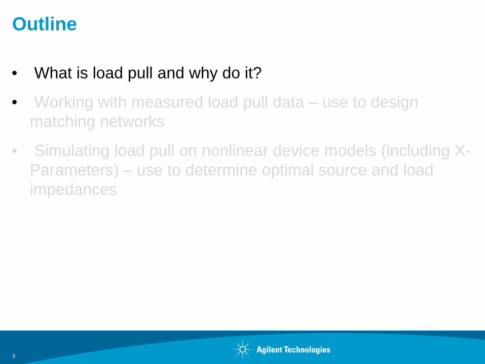
Outline
• What is load pull and why do it?
• Working with measured load pull data – use to design matching networks
• Simulating load pull on nonlinear device models (including X-Parameters) – use to determine optimal source and load impedances
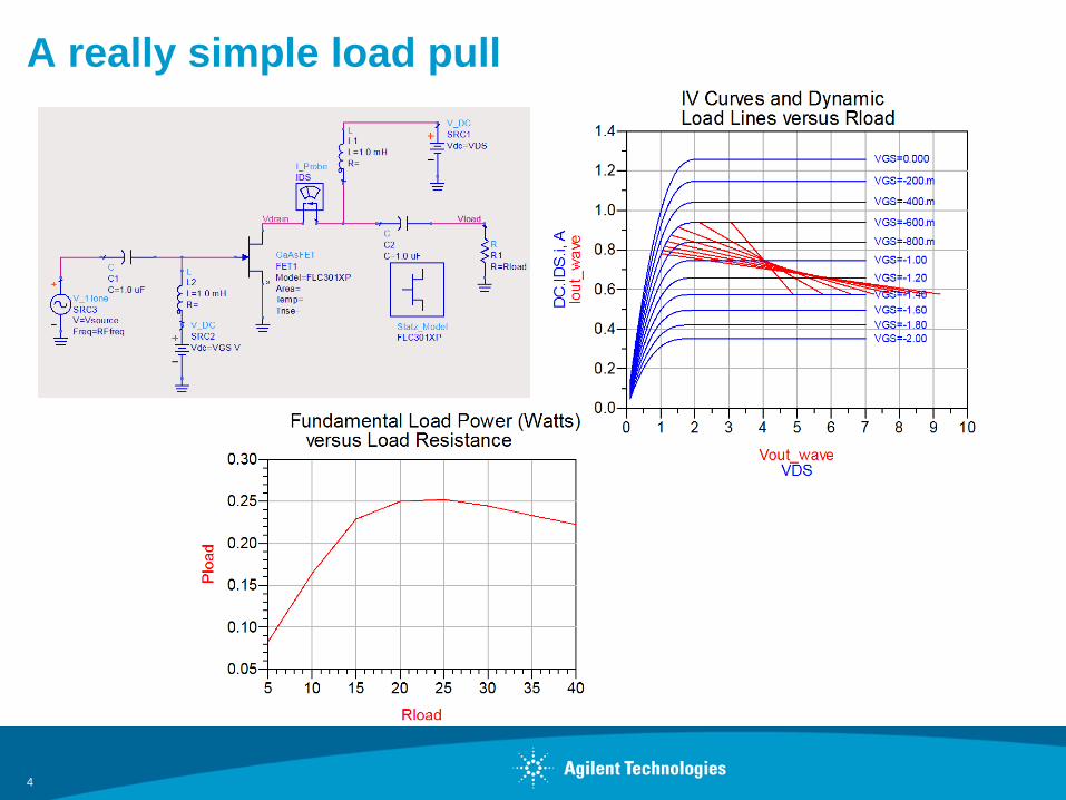
A really simple load pull
4

Device performance depends on source and load impedances
5
Input match.network
Output match.network
freqf1 f2 f3
freqf1 f2 f3
Externalload (or next stage)
Externalsource (or previous stage)
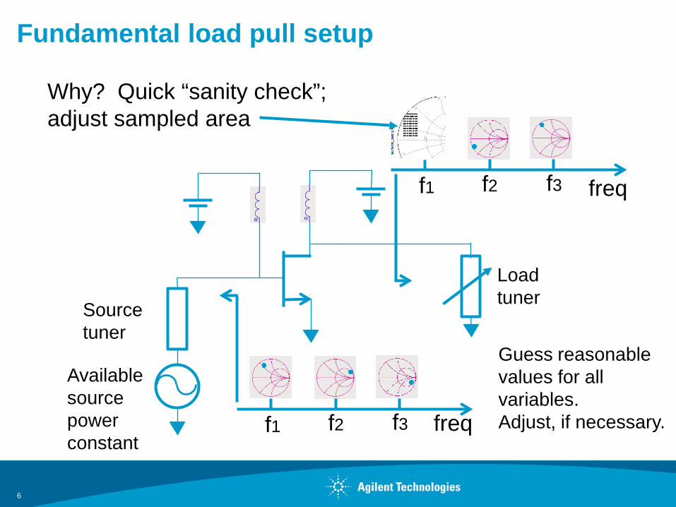
Fundamental load pull setup
6
freqf1 f2 f3
freqf1 f2 f3
Load tunerSource
tuner
Available source power constant
Why? Quick “sanity check”; adjust sampled area
Guess reasonablevalues for allvariables.Adjust, if necessary.

Fundamental load pull – with power sweep
7
freqf1 f2 f3
freqf1 f2 f3
Load tunerSource
tuner
Available source power swept freq
Why? See gain compression and constant powerdelivered data

Fundamental source pull setup
8
freqf1 f2 f3
freqf1 f2 f3
Load tuner
Source tuner
Available source power constant
Why? Source impedances affect performances, too
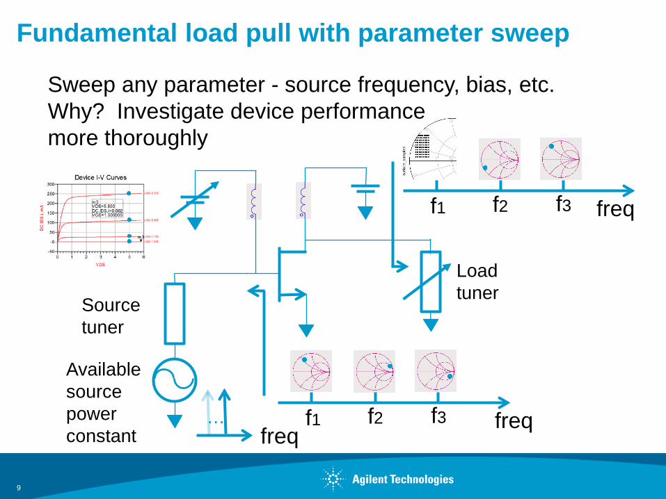
Fundamental load pull with parameter sweep
9
freqf1 f2 f3
freqf1 f2 f3
Load tunerSource
tuner
Available source power constant
…
Sweep any parameter - source frequency, bias, etc.Why? Investigate device performancemore thoroughly
freq
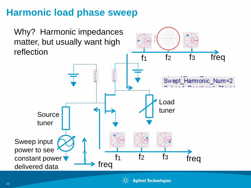
Harmonic load phase sweep
10
freqf1 f2 f3
freqf1 f2 f3
Load tunerSource
tuner
freq
Sweep input power to see constant powerdelivered data
Why? Harmonic impedancesmatter, but usually want highreflection
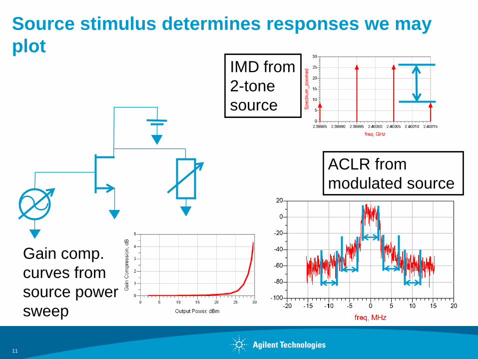
Source stimulus determines responses we may plot
11
Gain comp.curves from source powersweep
IMD from2-tonesource
ACLR frommodulated source

Constant power delivered load pull with parameter sweep – more precise characterization
12
freqf1 f2 f3
freqf1 f2 f3
Load tuner
Source tuner
Available source power optimized
…
Sweep any parameter - source frequency, bias, etc.
freq
Power deliveredheld constantvia optimization
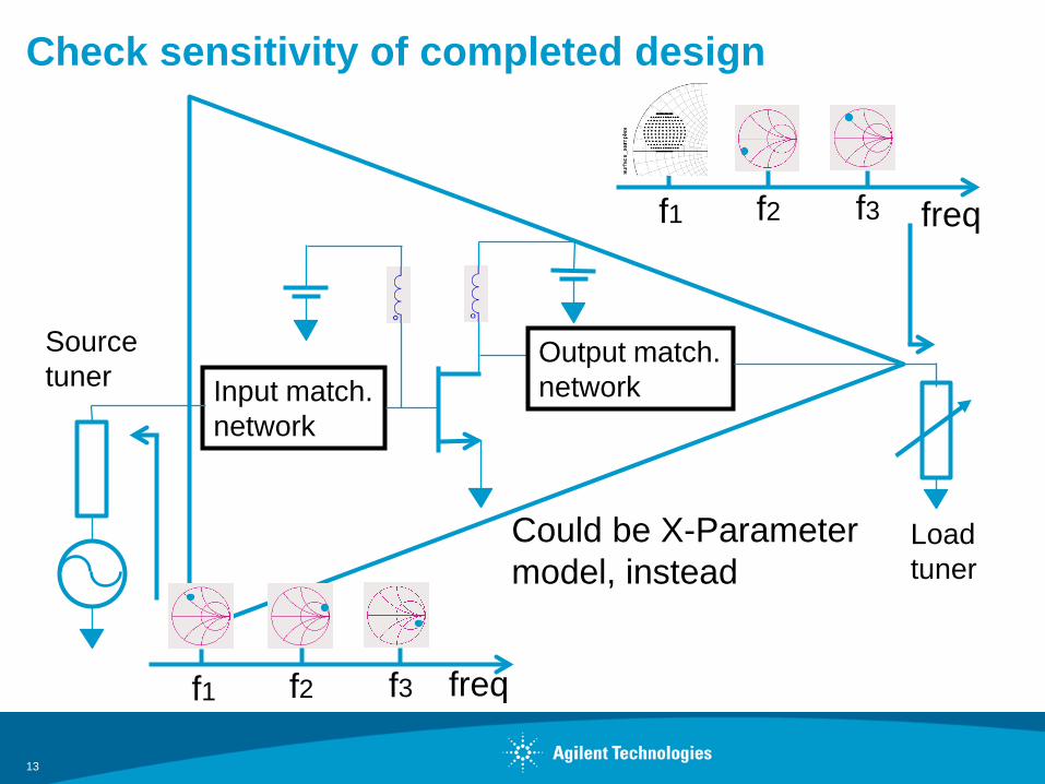
Check sensitivity of completed design
13
Input match.network
Output match.network
freqf1 f2 f3
freqf1 f2 f3
Loadtuner
Sourcetuner
Could be X-Parametermodel, instead

14
Outline
• What is load pull and why do it?
• Working with measured load pull data – use to design matching networks
• Simulating load pull on nonlinear device models (including X-Parameters) – use to determine optimal source and load impedances

You have measured load pull data (Maury)
15
What’s the optimal load? What performance can we get from this device?
16

Examine performance contours
17
1) Reads LP data file2) Simulates S-parameters
of network3) Gets corresponding
performance data Tuner generates loads in region you specify

View independent variables and performance parameters
18
Frequency andinput power constant
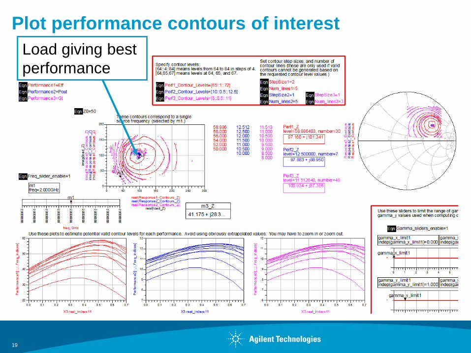
Plot performance contours of interest
19
Load giving best performance
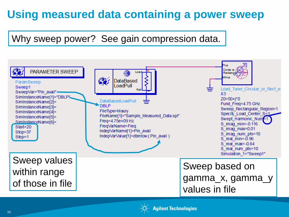
Using measured data containing a power sweep
20
Sweep valueswithin rangeof those in file
Sweep based ongamma_x, gamma_yvalues in file
Why sweep power? See gain compression data.
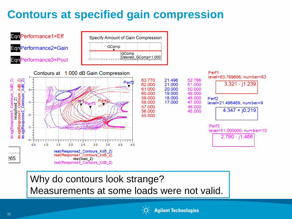
Contours at specified gain compression
21
Why do contours look strange? Measurements at some loads were not valid.

Contours at a particular input power
22
From contours we decide optimal impedances. What’s next?
23
Design impedance matching network(s) using existing techniques, or…

Use measured data directly in optimization
24
This impedance should bethe same as this.
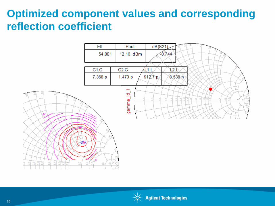
Optimized component values and corresponding reflection coefficient
25

26
Outline
• What is load pull and why do it?
• Working with measured load pull data – use to design matching networks
• Simulating load pull on nonlinear device models (including X-Parameters) – use to determine optimal source and load impedances
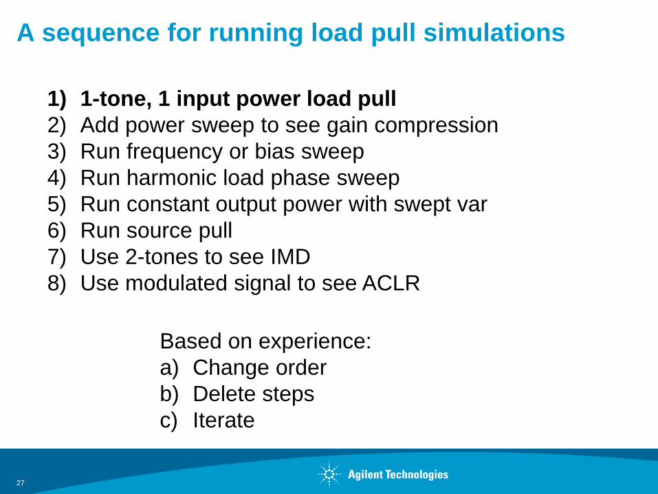
A sequence for running load pull simulations
27
1) 1-tone, 1 input power load pull2) Add power sweep to see gain compression3) Run frequency or bias sweep4) Run harmonic load phase sweep5) Run constant output power with swept var6) Run source pull7) Use 2-tones to see IMD8) Use modulated signal to see ACLR
Based on experience:a) Change orderb) Delete stepsc) Iterate
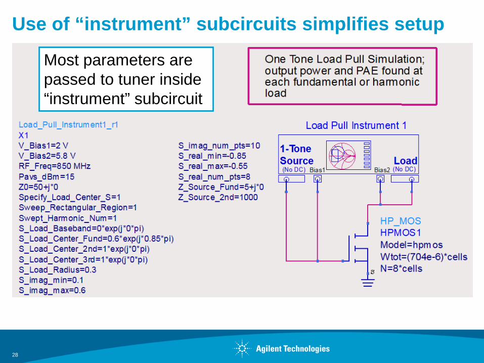
Use of “instrument” subcircuits simplifies setup
28
Most parameters are passed to tuner inside “instrument” subcircuit
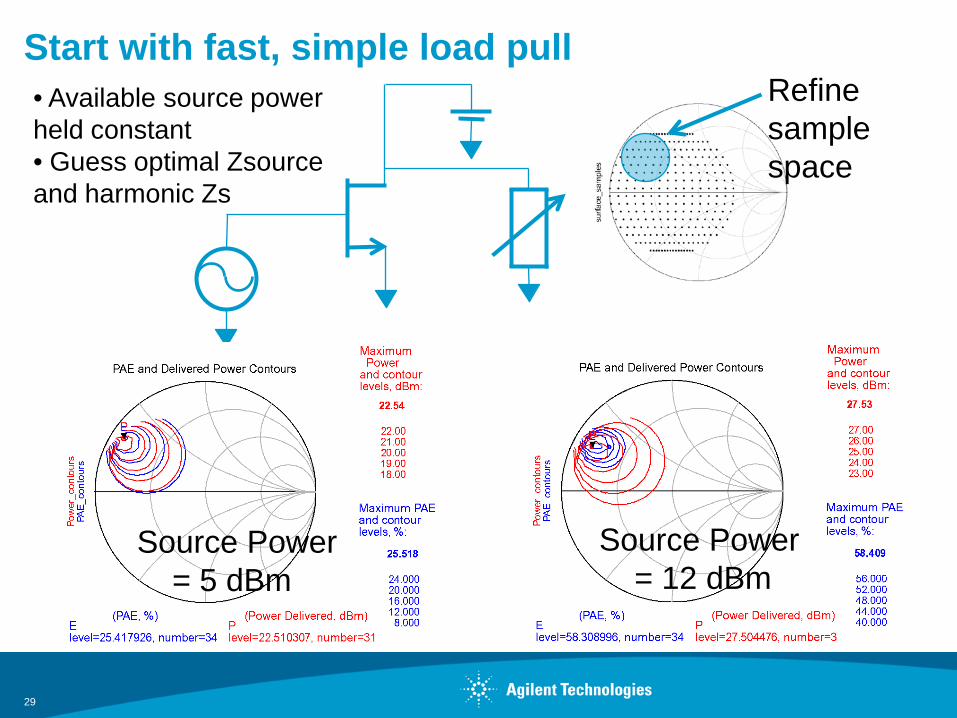
Start with fast, simple load pull
29
Source Power= 5 dBm
Source Power= 12 dBm
Refine sample space
• Available source power held constant• Guess optimal Zsource and harmonic Zs

A sequence for running load pull simulations
30
1) 1-tone, 1 input power load pull2) Add power sweep to see gain compression3) Run frequency or bias sweep4) Run harmonic load phase sweep5) Run constant output power with swept var6) Run source pull7) Use 2-tones to see IMD8) Use modulated signal to see ACLR
Based on experience:a) Change orderb) Delete stepsc) Iterate
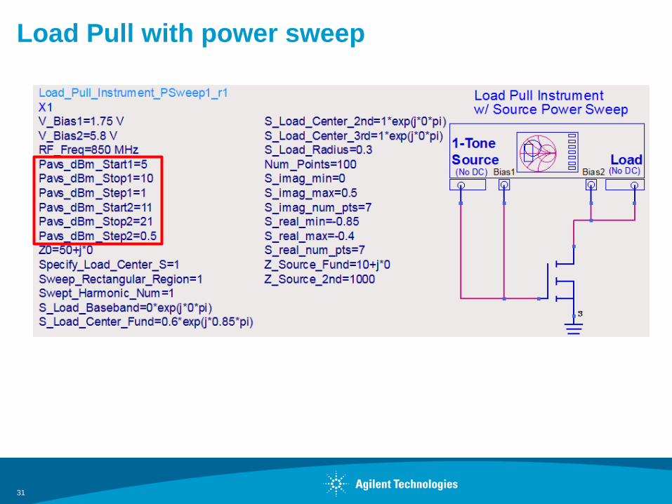
Load Pull with power sweep
31
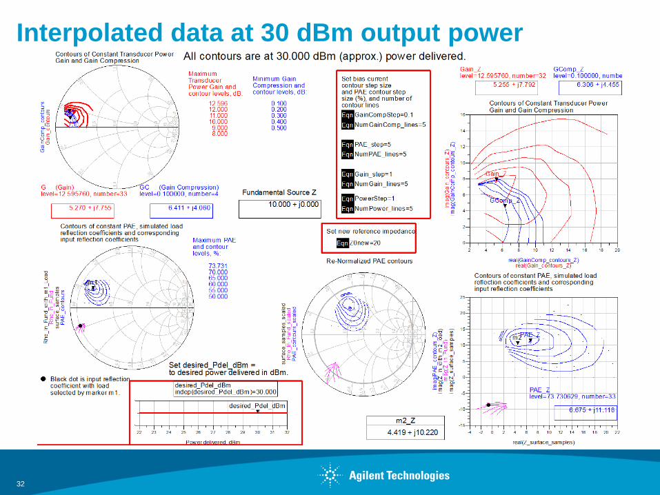
Interpolated data at 30 dBm output power
32
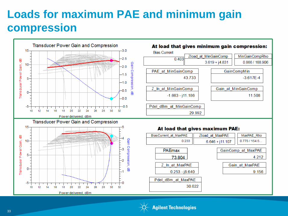
Loads for maximum PAE and minimum gain compression
33
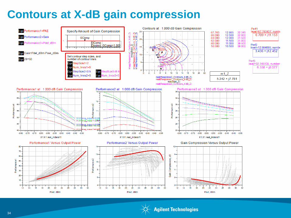
Contours at X-dB gain compression
34

Adjusting contour lines to all pass through maximum PAE load
35
Maximum PAE (Perf1 marker) occurs with 28.8 dBm power delivered (Perf3 contour) and 12.3 dB gain(Perf2 contour.)

A sequence for running load pull simulations
36
1) 1-tone, 1 input power load pull2) Add power sweep to see gain compression3) Run frequency or bias sweep4) Run harmonic load phase sweep5) Run constant output power with swept var6) Run source pull7) Use 2-tones to see IMD8) Use modulated signal to see ACLR
Based on experience:a) Change orderb) Delete stepsc) Iterate
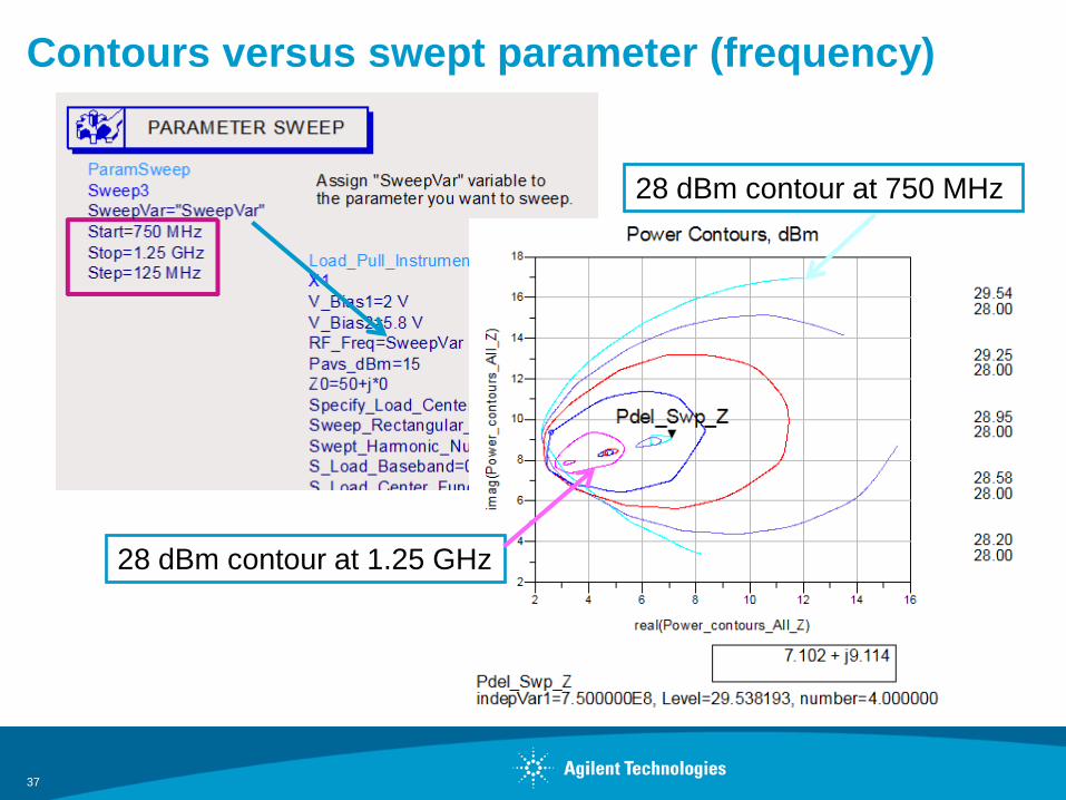
Contours versus swept parameter (frequency)
37
28 dBm contour at 750 MHz
28 dBm contour at 1.25 GHz

A sequence for running load pull simulations
38
1) 1-tone, 1 input power load pull2) Add power sweep to see gain compression3) Run frequency or bias sweep4) Run harmonic load phase sweep5) Run constant output power with swept var6) Run source pull7) Use 2-tones to see IMD8) Use modulated signal to see ACLR
Based on experience:a) Change orderb) Delete stepsc) Iterate

Dependency on phase of gamma at harmonic(s)
39
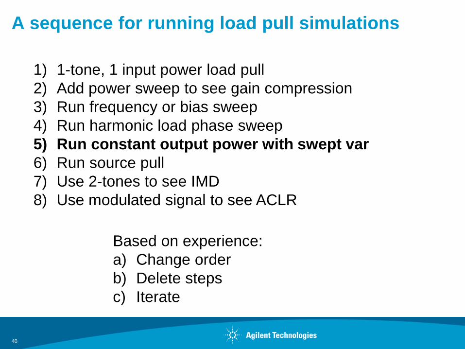
A sequence for running load pull simulations
40
1) 1-tone, 1 input power load pull2) Add power sweep to see gain compression3) Run frequency or bias sweep4) Run harmonic load phase sweep5) Run constant output power with swept var6) Run source pull7) Use 2-tones to see IMD8) Use modulated signal to see ACLR
Based on experience:a) Change orderb) Delete stepsc) Iterate
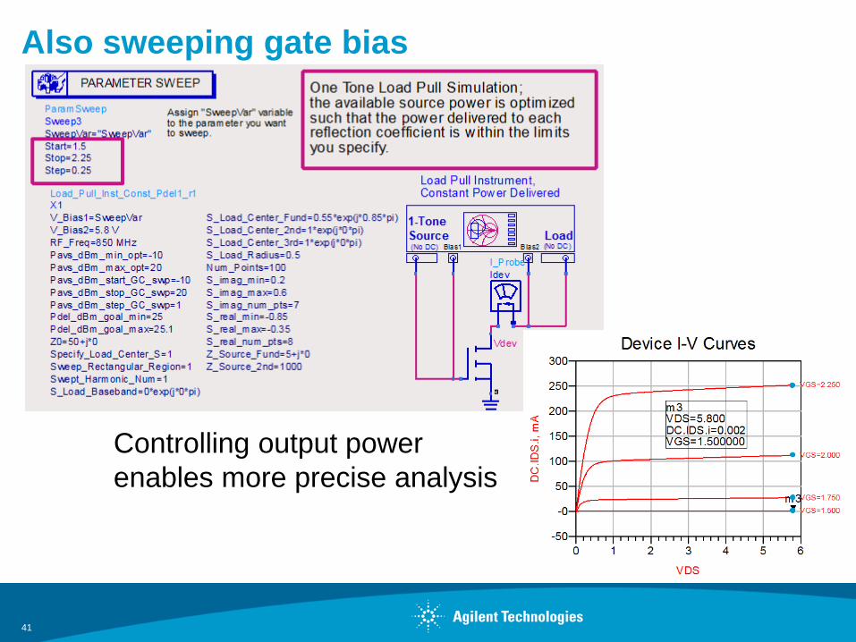
Also sweeping gate bias
41
Controlling output powerenables more precise analysis
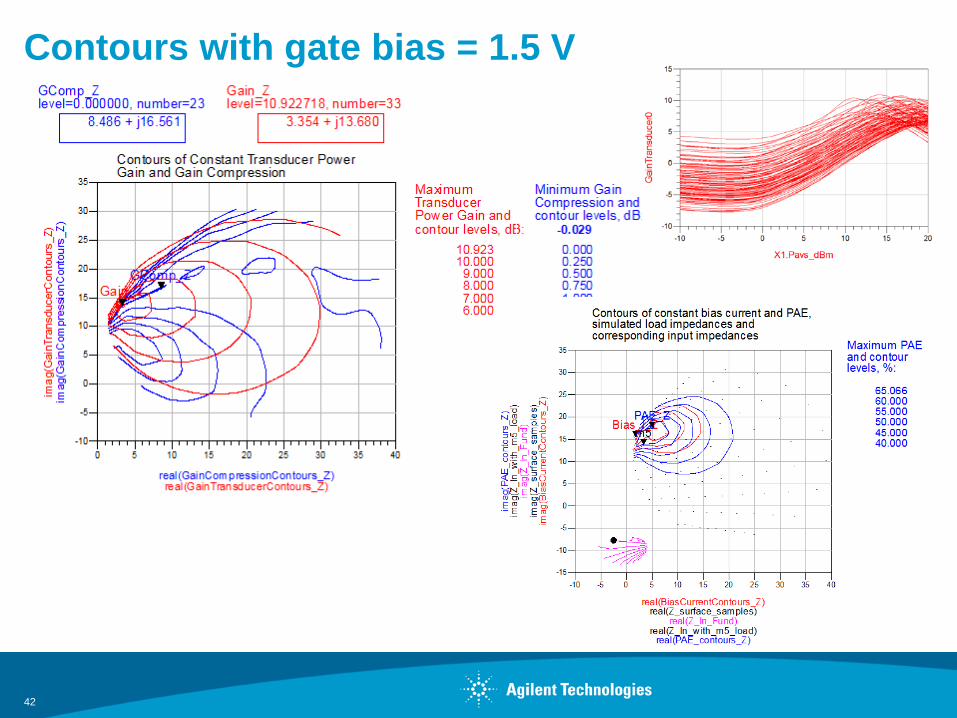
Contours with gate bias = 1.5 V
42

High PAE, but low gain
43
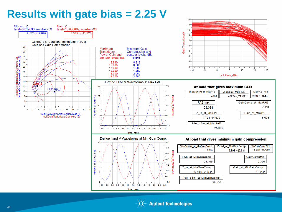
Results with gate bias = 2.25 V
44
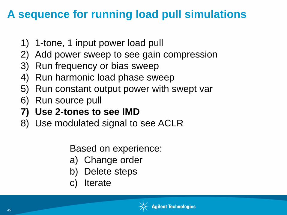
A sequence for running load pull simulations
45
1) 1-tone, 1 input power load pull2) Add power sweep to see gain compression3) Run frequency or bias sweep4) Run harmonic load phase sweep5) Run constant output power with swept var6) Run source pull7) Use 2-tones to see IMD8) Use modulated signal to see ACLR
Based on experience:a) Change orderb) Delete stepsc) Iterate
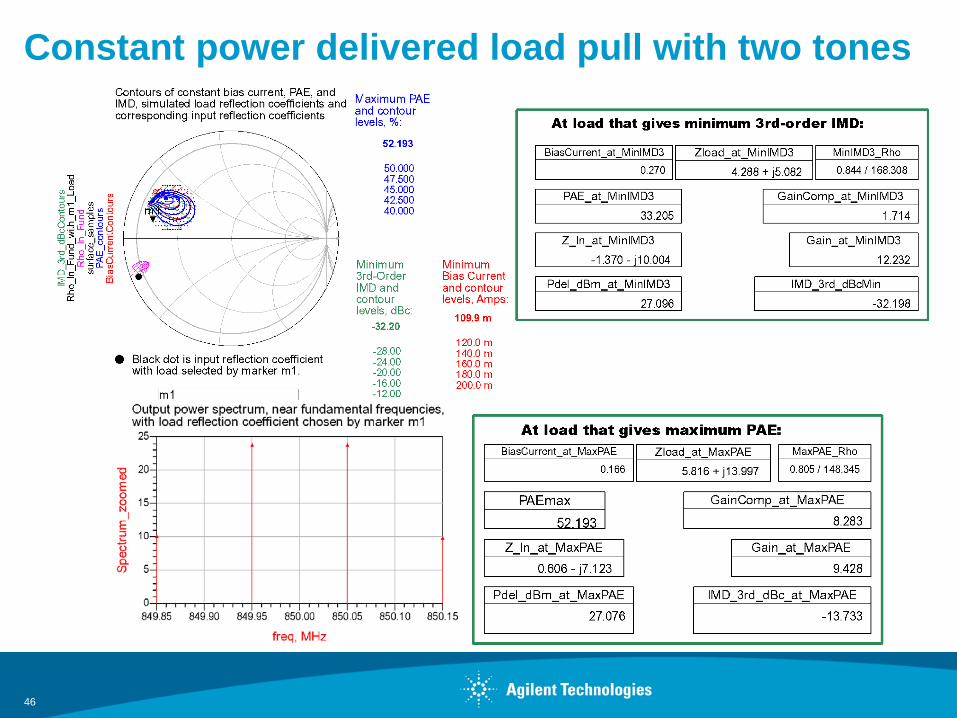
Constant power delivered load pull with two tones
46

A sequence for running load pull simulations
47
1) 1-tone, 1 input power load pull2) Add power sweep to see gain compression3) Run frequency or bias sweep4) Run harmonic load phase sweep5) Run constant output power with swept var6) Run source pull7) Use 2-tones to see IMD8) Use modulated signal to see ACLR
Based on experience:a) Change orderb) Delete stepsc) Iterate
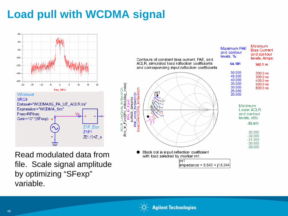
Load pull with WCDMA signal
48
Read modulated data from file. Scale signal amplitude by optimizing “SFexp” variable.

49
Review
• Basic load pull concepts
• Using measured load pull data files to design matching networks
• Fast, simple load pull
• Adding power sweeps to see compression
• Sweeping frequency
• Sweeping harmonic reflection coefficient phase
• Constant power-delivered load pull with sweep
• Using two tones to see intermodulation distortion
• Load pull with a WCDMA source

For more information:
50
http://edocs.soco.agilent.com/display/eesofkc/Load+Pull+DesignGuide+Enhancements+for+post+ADS+2011_05
On the latest release of ADS:
http://www.agilent.com/find/eesof-ads
On the latest release of the ADS Load Pull DesignGuide:

For more information aboutAgilent EEsof EDA, visit:
www.agilent.com/find/eesof-ads
For more information on Agilent Technologies’products, applications or services, pleasecontact your local Agilent office. Thecomplete list is available at:
www.agilent.com/find/contactus
Contact Agilent at:
AmericasCanada (877) 894-4414Brazil (11) 4197 3500Mexico 01800 5064 800United States (800) 829-4444
Asia PacificAustralia 1 800 629 485China 800 810 0189Hong Kong 800 938 693India 1 800 112 929Japan 0120 (421) 345Korea 080 769 0800Malaysia 1 800 888 848Singapore 1 800 375 8100Taiwan 0800 047 866Thailand 1 800 226 008
Europe & Middle East
Austria 01 36027 71571Belgium 32 (0) 2 404 93 40Denmark 45 70 13 1515Finland 358 (0) 10 855 2100France 0825 010 700*
*0.125 €/minuteGermany 07031 464 6333Ireland 1890 924 204Israel 972-3-9288-504/544Italy 39 02 92 60 8484Netherlands 31 (0) 20 547 2111Spain 34 (91) 631 3300Sweden 0200-88 22 55Switzerland 0800 80 53 53United Kingdom 44 (0) 131 452 0200Other European Countries:www.agilent.com/find/contactus
Product specifications and descriptions in this document subject to change without notice.
© Agilent Technologies, Inc. 2011Published in USA, November 8, 20115990-9506EN
www.agilent.com